Learning with Delayed Payoffs in Population Games
using Kullback-Leibler Divergence Regularization

Abstract

We study a multi-agent decision problem in large population games. Agents across multiple populations select strategies for repeated interactions with one another. At each stage of the interactions, agents use their decision-making model to revise their strategy selections based on payoffs determined by an underlying game. Their goal is to learn the strategies of the Nash equilibrium of the game. However, when games are subject to time delays, conventional decision-making models from the population game literature result in oscillation in the strategy revision process or convergence to an equilibrium other than the Nash. To address this problem, we propose the Kullback-Leibler Divergence Regularized Learning (KLD-RL) model and an algorithm to iteratively update the model’s regularization parameter. Using passivity-based convergence analysis techniques, we show that the KLD-RL model achieves convergence to the Nash equilibrium, without oscillation, for a class of population games that are subject to time delays. We demonstrate our main results numerically on a two-population congestion game and a two-population zero-sum game.

I Introduction

Consider a large number of agents engaged in repeated strategic interactions. Each agent selects a strategy for the interactions but can repeatedly revise its strategy according to payoffs determined by an underlying payoff mechanism. To learn and adopt the best strategy without knowing the structure of the payoff mechanism, the agent needs to revise its strategy selection at each stage of the interactions based on the instantaneous payoffs it receives.

This multi-agent decision problem is relevant in control engineering applications where the goal is to design decision-making models for multiple agents to learn effective strategy selections in a self-organized way. Applications include computation offloading over communication networks [1], user association in cellular networks [2], multi-robot task allocation [3], demand response in smart grids [4, 5], water distribution systems [6, 7], building temperature control [8], wireless networks [9], electric vehicle charging [10], distributed control systems [11], and distributed optimization [12].

To formalize the problem, we adopt the population game framework [13, Chapter 2]. In this framework, a payoff function defines how the payoffs are determined based on the agents’ strategy profile, which is the distribution of their strategy selections over a finite number of available strategies. An evolutionary dynamic model describes how individual agents revise their strategies to increase the payoffs they receive. A key research theme is in establishing convergence of the strategy profile to the Nash equilibrium where no agent is better off by unilaterally revising its strategy selection.

Unlike in existing studies, we investigate scenarios where the payoff mechanism is subject to time delays. This models, for example, propagation of traffic congestion on roads in congestion games [16], delay in communication between electric power utility and demand response agents in demand response games [4], and limitations of agents in sensing link status in network games [17]. When agents revise their strategy selections based on delayed payoffs, the strategy profile does not converge to the Nash equilibrium. In fact, prior work in the game theory literature [18, 19, 20, 21, 22, 23, 24, 25, 26, 27, 28, 29, 30, 31, 32, 33] suggests that when multi-agent games are subject to time delays, the strategy profile oscillates under many of existing decision-making models.

As a main contribution of this paper, we propose a new class of decision-making models called the Kullback-Leibler Divergence Regularized Learning (KLD-RL). The main idea behind the new model is to regularize the agents’ decision making using the Kullback-Leibler divergence. Such regularization makes the agent strategy revision insensitive to time delays in the payoff mechanism. This prevents the strategy profile from oscillating, and through successive updates of the model’s regularization parameter, it ensures that the agents improve their strategy selections. As a consequence, when the agents revise strategy selections based on the proposed model, their strategy profile is guaranteed to converge to the Nash equilibrium in a certain class of population games.

The logit dynamics model [34, 35] is known to converge to an equilibrium state in a large class of population games, including games subject to time delays [36, 37]. However, as discussed in [35], the equilibrium state of the logit dynamics model is a perturbed version of the Nash equilibrium. This forces the agents to select sub-optimal strategies, for instance, in potential games [38, 39] with concave payoff potentials, where the Nash equilibrium is the socially optimal strategy profile. Such a significant limitation in existing models motivates our investigation of a new decision-making model.

Below we summarize the main contributions of this paper.

• We propose a parameterized class of KLD-RL models that generalize the existing logit dynamics model. We explain how the new model implements the idea of regularization in multi-agent decision making, and provide an algorithm that iteratively updates the model’s regularization parameter.

• Leveraging stability results from recent works on higher-order learning in large population games [37, 36], we discuss, under the KLD-RL model, the convergence of the strategy profile to the Nash equilibrium in an important class of population games, widely known as contractive population games [40].

• We present numerical simulations using multi-population games to demonstrate how the new model ensures the convergence to the Nash equilibrium, despite time delays in the games. Using simulation outcomes, we illustrate how our main convergence results are different from those of the existing logit model and highlight the importance of the proposed model in applications.

The paper is organized as follows. In Section II, we explain the multi-agent decision problem addressed in this paper. In Section III, we provide a comparative review of related works. In Section IV, we introduce the KLD-RL model and explain how to iteratively update the model’s regularization parameter. We present our main theorem that establishes the convergence of the strategy profile determined by the model to the Nash equilibrium in a certain class of contractive population games. In Section V, we present simulation results that demonstrate the effectiveness of the proposed model in learning and converging to the Nash equilibrium. We discuss interesting extensions of our finding in Section VI and conclude the paper with a summary and future directions in Section VII.

II Problem Description

$\mathbb{R}^{n}$	set of $n$-dimensional real vectors.
$\mathbb{R}^{n}_{+}$	set of $n$-dimensional nonnegative real vectors.
$\mathbb{X}^{k},\mathbb{X}$	state spaces of population $k$ and the society.
$T\mathbb{X}^{k},T\mathbb{X}$	tangent spaces of $\mathbb{X}^{k}$ and $\mathbb{X}$.
$\mathrm{int}(\mathbb{X}^{k}),\mathrm{int}(\mathbb{X})$	interiors of $\mathbb{X}^{k}$ and $\mathbb{X}$ defined, respectively, as
	$\mathrm{int}(\mathbb{X}^{k})=\{x^{k}\in\mathbb{X}^{k}\,|\,x_{i}^{k}>0,\,1\leq i\leq n^{k}\}$ and
	$\mathrm{int}(\mathbb{X})=\mathrm{int}(\mathbb{X}^{1})\times\cdots\times\mathrm{int}(\mathbb{X}^{M})$.
$\mathcal{F},D\mathcal{F}$	payoff function of a population game and its differential map.
$\mathbb{NE}\left(\mathcal{F}\right)$	Nash equilibrium set of a population game $\mathcal{F}$, defined as in (1).
$\mathbb{PNE}_{\eta,\theta}\left(\mathcal{F}\right)$	perturbed Nash equilibrium set of a population game $\mathcal{F}$, defined as in (26).
$\mathcal{D}(x\,\|\,y)$	Kullback-Leibler divergence defined as $\sum_{i=1}^{n}x_{i}\ln\frac{x_{i}}{y_{i}}$ for (element-wise) nonnegative vectors $x=(x_{1},\cdots,x_{n})$ and $y=(y_{1},\cdots,y_{n})$.

TABLE I: List of basic notation

Consider a society consisting of $M$ populations of decision-making agents. We denote by $\{1,\cdots,M\}$ the populations constituting the society and by $\{1,\cdots,n^{k}\}$ the set of strategies available to agents in each population $k$. Let $x^{k}(t)=(x_{1}^{k}(t),\cdots,x_{n^{k}}^{k}(t))$ be a $n^{k}$-dimensional nonnegative real-valued vector where each entry $x_{i}^{k}(t)$ denotes the portion of population $k$ adopting strategy $i$ at time instant $t$. We refer to $x^{k}(t)$ as the state of population $k$ and constant $m^{k}=\textstyle\sum_{i=1}^{n^{k}}x_{i}^{k}(t),~{}\forall t\geq 0$ as the mass of the population. Also, by aggregating the states of all populations, we define the social state $x(t)=(x^{1}(t),\cdots,x^{M}(t))$ which describes the strategy profiles across all $M$ populations at time $t$. Let $n$ be the total number of strategies available in the society, i.e, $n=\sum_{k=1}^{M}n^{k}$. We denote the space of viable population states as $\mathbb{X}^{k}=\{x^{k}\in\mathbb{R}_{+}^{n^{k}}\,\big{|}\,\textstyle\sum_{i=1}^{n^{k}}x_{i}^{k}=m^{k}\}$. Accordingly, we define $\mathbb{X}=\mathbb{X}^{1}\times\cdots\times\mathbb{X}^{M}$ as the space of viable social states. For concise presentation, without loss of generality, we assume that $m^{k}=1,~{}\forall k\in\{1,\cdots,M\}$.

In what follows, we review relevant definitions from the population games literature. Table I summarizes the basic notation used throughout the paper. For all variables and parameters adopted in this paper, the superscript is used to indicate their association with an indicated population.

II-A Population Games and Time Delays in Payoff Mechanisms

II-A1 Population games

We denote the payoffs assigned to each population $k$ at time instant $t$ by an $n^{k}$-dimensional real-valued vector $p^{k}(t)=(p_{1}^{k}(t),\cdots,p_{n^{k}}^{k}(t))\in\mathbb{R}^{n^{k}}$. Each $p_{i}^{k}(t)$ represents the payoff given to the agents in population $k$ selecting strategy $i$. We denote by $p(t)=(p^{1}(t),\cdots,p^{M}(t))\in\mathbb{R}^{n}$ the payoffs assigned to the agents in the entire society. According to the conventional definition, a population game is associated with a payoff function $\mathcal{F}=(\mathcal{F}^{1},\cdots,\mathcal{F}^{M})$ with $\mathcal{F}^{k}:\mathbb{X}\to\mathbb{R}^{n^{k}}$ which assigns a payoff vector to each population $k$ as $p^{k}(t)=\mathcal{F}^{k}(x(t))$, where $x(t)\in\mathbb{X}$ is the social state at time $t$. We adopt the definition of the Nash equilibrium of $\mathcal{F}$ as follows.

Definition 1 (Nash Equilibrium)

An element $z^{\footnotesize\text{NE}}$ in $\mathbb{X}$ is called the Nash equilibrium of the population game $\mathcal{F}$ if it satisfies the following condition:

$$(z^{\footnotesize\text{NE}}-z)^{T}\mathcal{F}(z^{\footnotesize\text{NE}})\geq 0,~{}\forall z\in\mathbb{X}.$$ (1)

Population games can have multiple Nash equilibria. We denote by $\mathbb{NE}(\mathcal{F})$ the set of all Nash equilibria of $\mathcal{F}$.

Below, we provide examples of population games and identify their unique Nash equilibrium. The examples will be used in Section V to illustrate our main results.

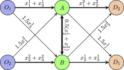
Figure 1: Two-Population Congestion Game: Agents in each population $k$ traverse from origin $O_{k}$ to destination $D_{k}$ using one of the following routes: $O_{1}\to A\to D_{1}$ (Route 1), $O_{1}\to A\to B\to D_{1}$ (Route 2), and $O_{1}\to B\to D_{1}$ (Route 3) for population 1; $O_{2}\to A\to D_{2}$ (Route 1), $O_{2}\to B\to A\to D_{2}$ (Route 2), and $O_{2}\to B\to D_{2}$ (Route 3) for population 2. We assume that with the same number of agents on the links, the diagonal links ($O_{1}\to B,O_{2}\to A,A\to D_{1},B\to D_{2}$) are $50\%$ more congested than the horizontal links, e.g, the roads represented by the diagonal links are narrower; whereas the vertical link $A\leftrightarrow B$ is $50\%$ less congested than the horizontal links, e.g., the road associated with the vertical link is wider. The different weights on the links reflect such assumption.

Example 1

Consider a congestion game with two populations ($M=2$) where each population is assigned a fixed origin and destination. To reach their respective destinations, agents in each population use one of three available routes as depicted in Fig. 1. We consider the game scenario where every agent needs to repeatedly travel from its origin to destination, e.g., to commute to work on every workday. Each strategy in the game is defined as an agent taking one of the available routes. Its associated payoff reflects the level of congestion along the selected route, which depends on the number of agents from possibly both populations using the route. To formalize this, we adopt the payoff function $\mathcal{F}=(\mathcal{F}^{1},\mathcal{F}^{2})$ defined as

$$\mathcal{F}^{1}(x^{1},x^{2}) =-\begin{pmatrix}2.5x_{1}^{1}+x_{2}^{1}\\ x_{1}^{1}+2.5x_{2}^{1}+x_{3}^{1}+0.5x_{2}^{2}\\ x_{2}^{1}+2.5x_{3}^{1}\end{pmatrix}$$ (2a)

$$\mathcal{F}^{2}(x^{1},x^{2}) =-\begin{pmatrix}2.5x_{1}^{2}+x_{2}^{2}\\ 0.5x_{2}^{1}+x_{1}^{2}+2.5x_{2}^{2}+x_{3}^{2}\\ x_{2}^{2}+2.5x_{3}^{2}\end{pmatrix}.$$ (2b)

We note that (2) has the unique Nash equilibrium $x^{\footnotesize\text{NE}}=\left(4/9,1/9,4/9,4/9,1/9,4/9\right)$ at which the average congestion level across all six routes is minimized. ∎

Example 2

Consider a two-population zero-sum game whose payoff function $\mathcal{F}=(\mathcal{F}^{1},\mathcal{F}^{2})$ is derived from a biased Rock-Paper-Scissors (RPS) game [41] as follows:

$$\mathcal{F}^{1}(x^{1},x^{2}) =\begin{pmatrix}-0.5x_{2}^{2}+x_{3}^{2}\\ 0.5x_{1}^{2}-0.1x_{3}^{2}\\ -x_{1}^{2}+0.1x_{2}^{2}\end{pmatrix}$$ (3a)

$$\mathcal{F}^{2}(x^{1},x^{2}) =\begin{pmatrix}-0.5x_{2}^{1}+x_{3}^{1}\\ 0.5x_{1}^{1}-0.1x_{3}^{1}\\ -x_{1}^{1}+0.1x_{2}^{1}\end{pmatrix}.$$ (3b)

The study of zero-sum games has an important implication in security-related applications. For example, attacker-defender (zero-sum) game formulations [42, 43] can be used to predict an attacker’s strategy at the Nash equilibrium and to design the best defense strategy.

Agents in each population $k=1,2$ can select one of three strategies: rock ($x_{1}^{k}$), paper ($x_{2}^{k}$), or scissors ($x_{3}^{k}$). The payoffs $\mathcal{F}^{k}(x^{1},x^{2})$ assigned to each population $k$ reflect the chances of winning the game against its opponent population, as illustrated in Fig. 2. The agents are engaged in a multi-round game in which, based on the payoffs received in a previous round, they would revise strategy selections at each round of the game. Note that the game has the unique Nash equilibrium $x^{\footnotesize\text{NE}}=(1/16,10/16,5/16,1/16,10/16,5/16)$ at which each population minimizes the opponent population’s maximum gain (or equivalently maximizes its worst-case (minimum) gain). ∎

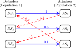
Figure 2: Two-Population Zero-Sum Game: Agents in the defender population (population 1) select defending strategies $(DS_{1},DS_{2},DS_{3})$ to play against those in the attacker population (population 2) who adopt attacking strategies $(AS_{1},AS_{2},AS_{3})$. The positive (negative) weight on the blue (red dotted) arrow between $DS_{i}$ and $AS_{j}$ denotes the reward (loss) associated with population 1 when the defenders and attackers adopt $DS_{i}$ and $AS_{j}$, respectively. The payoff $\mathcal{F}^{1}_{i}(x^{1},x^{2})$ associated with $DS_{i}$ of population 1 is the sum of the reward and loss when $x^{2}$ is the state of population 2; whereas the payoff $\mathcal{F}^{2}_{j}(x^{1},x^{2})$ associated with $AS_{j}$ of population 2 is the sum of the reward and loss when $x^{1}$ is the state of population 1.

We make the following assumption on payoff function $\mathcal{F}$.

Assumption 1

The differential map $D\mathcal{F}$ of $\mathcal{F}$ exists and is continuous on $\mathbb{X}$, and both $\mathcal{F}$ and $D\mathcal{F}$ are bounded: there are $B_{\mathcal{F}}$ and $B_{D\mathcal{F}}$ satisfying $B_{\mathcal{F}}=\max_{z\in\mathbb{X}}\|\mathcal{F}(z)\|_{2}$ and $B_{D\mathcal{F}}=\max_{z\in\mathbb{X}}\|D\mathcal{F}(z)\|_{2}$, respectively.

Note that any affine payoff function $\mathcal{F}(x)=Fx+b$ with $F\in\mathbb{R}^{n\times n},b\in\mathbb{R}^{n}$, e.g., (2), (3), satisfies Assumption 1. Contractive population games are defined as follows.

Definition 2 (Contractive Population Game [40])

A population game $\mathcal{F}$ is called contractive if it holds that

$$\left(w-z\right)^{T}\left(\mathcal{F}\left(w\right)-\mathcal{F}\left(z\right)\right)\leq 0,~{}\forall w,z\in\mathbb{X}.$$ (4)

In particular, if the equality holds if and only if $w=z$, $\mathcal{F}$ is called strictly contractive.

If a population game $\mathcal{F}$ is contractive, then its Nash equilibrium set $\mathbb{NE}(\mathcal{F})$ is convex; moreover, if $\mathcal{F}$ is strictly contractive, then it has a unique Nash equilibrium [40, Theorem 13.9]. For the affine payoff function $\mathcal{F}(x)=Fx+b$, the requirement (4) is equivalent to the negative semi-definiteness of $F$ in the tangent space $T\mathbb{X}$ of $\mathbb{X}$. Both games in Examples 1 and 2 are contractive. We call $\mathcal{F}$ a contractive potential game if there is a concave potential function $f$ satisfying $\mathcal{F}=\nabla f$ in which case the Nash equilibrium attains the minimum of $f$. The congestion game (2) is a contractive potential game and the Nash equilibrium attains the minimum average congestion.

II-A2 Time delays in payoff mechanisms

Unlike in the standard formulation explained in Section II-A1, in this work, the payoff vector at each time instant depends not only on the current but also past social states to capture time delays in the payoff mechanism underlying a population game. Adopting [45, Definition 1.1.3], we denote such dependency by

$$p(t)=\left(\mathfrak{G}x\right)(t),$$ (5)

where $\mathfrak{G}$ is a causal mapping. We require that when $x(t)$ converges, i.e., $\lim_{t\to\infty}x(t)=\bar{x}$, so does $p(t)$, i.e., $\lim_{t\to\infty}p(t)=\mathcal{F}(\bar{x})$, where $\mathcal{F}$ is the payoff function of an underlying population game. Following the same naming convention as in [37], we refer to (5) as the payoff dynamics model (PDM). However, unlike the original definition of the PDM, described as a finite-dimensional dynamical system, (5) expands the existing PDM definition to include a certain type of infinite-dimensional systems such as (6) given below. In what follows, we provide two cases of population games with time delays that can be represented using (5).

Payoff Function with a Time Delay

Consider that the payoff vector $p(t)$ at time $t$ depends on the past social state $x(t-d)$ at time $t-d$:

$$p(t)=\mathcal{F}\left(x(t-d)\right),~{}t\geq d,$$ (6)

where the positive constant $d$ denotes a time delay and it holds that $p(t)=\mathcal{F}(x(0)),~{}0\leq t<d$. By the continuity of $\mathcal{F}$, when the social state $x(t)$ converges to $\bar{x}$, so does the payoff vector $p(t)$ to $\mathcal{F}(\bar{x})$. Note that (6) can be regarded as an infinite-dimensional dynamical system model.

We assume that $d$ is unknown to the agents, but they have an (estimated) upper bound $B_{d}$ of $d$. For instance, in the congestion game (Example 1), each agent’s gathering of information about the congestion level of available routes is subject to an unknown time delay, but the agent can make a good estimate of an upper bound on the time delay.

Smoothing Payoff Dynamics Model

We adopt similar arguments as in [36, Section V] to derive the smoothing PDM [37]. Suppose that the opportunity for the strategy revision of each agent in population $k$ occurs at each jump time of an independent and identically distributed Poisson process with parameter $1/N^{k}$, where $N^{k}$ is the number of agents in the population. At each strategy revision time, the agent receives a payoff associated with its revised strategy.

Let $t$ and $t+h$ be two consecutive strategy revision times. Note that by the definitions of the Poisson process and strategy revision time, $h$ goes to zero as $N^{k}$ tends to infinity. Given that the agent revises to strategy $j$ at time $t+h$ and receives a payoff $\mathcal{F}_{j}^{k}\left(x(t+h)\right)$, the population updates its payoff estimates for all available strategies as follows:

$$P_{i}^{k}(t\!+\!h)\!=\!\begin{cases}P_{i}^{k}(t)\!+\!h\lambda\frac{\mathcal{F}_{i}^{k}\left(x(t+h)\right)-P_{i}^{k}(t)}{\mathbb{P}\left(\text{agent selects strategy~{}$i$}\right)}&\!\text{if $i=j$}\\ P_{i}^{k}(t)&\!\text{otherwise.}\end{cases}$$ (7)

The variable $P_{i}^{k}(t)$ is the estimate of $\mathcal{F}_{i}^{k}(x(t))$ and the parameter $\lambda$ is the estimation gain. In expectation, (7) satisfies

$$\mathbb{E}\left(\frac{P_{i}^{k}(t\!+\!h)\!-\!P_{i}^{k}(t)}{h}\right)\!=\!-\lambda\mathbb{E}\left(P_{i}^{k}(t)\!-\!\mathcal{F}_{i}^{k}\left(x(t\!+\!h)\right)\right).$$ (8)

For a large number of agents, i.e., $N^{k}$ tends to infinity, we can approximate (8) with the following ordinary differential equation:

$$\dot{p}_{i}^{k}(t)=-\lambda\left(p_{i}^{k}(t)-\mathcal{F}_{i}^{k}\left(x(t)\right)\right).$$ (9)

The variable $p_{i}^{k}(t)$ can be viewed as an approximation of $\mathbb{E}(P_{i}^{k}(t))$. We refer to (9) as the smoothing PDM. Note that (9) can be interpreted as a low-pass filter applied to the signal $\mathcal{F}_{i}^{k}(x(t)),~{}t\geq 0$ and the filtering causes a time delay in computing the payoff estimates. Consequently, the filter output $p_{i}^{k}(t)$ lags behind the input $\mathcal{F}_{i}^{k}(x(t))$.

We make the following assumption on (5).

Assumption 2

The PDM (5) satisfies the technical conditions stated below.

1. Given that $\mathcal{F}$ is the payoff function of an underlying population game, (5) satisfies

   $$\lim_{t\to\infty}\left\|\dot{x}(t)\right\|_{2}\!=\!0\!\implies\!\lim_{t\to\infty}\left\|p(t)\!-\!\mathcal{F}(x(t))\right\|_{2}\!=\!0,$$

   where $p(t)$ is the payoff vector determined by (5) given a social state trajectory $x(t),~{}t\geq 0$.

2. Given a social state trajectory $x(t),~{}t\geq 0$, (5) computes a unique payoff vector trajectory $p(t),~{}t\geq 0$. In other words, for any pair of social state trajectories $x(t),~{}t\geq 0$ and $y(t),~{}t\geq 0$, it holds that

   $$x(t)=y(t),~{}\forall t\geq 0\\ \implies\left(\mathfrak{G}x\right)(t)=\left(\mathfrak{G}y\right)(t),~{}\forall t\geq 0.$$ (10)

3. If the social state trajectory $x(t),~{}t\geq 0$ is differentiable, so is the resulting payoff vector trajectory $p(t),~{}t\geq 0$. Given that $\dot{x}(t)$ is bounded, both $p(t)$ and $\dot{p}(t)$ are bounded, i.e., there exist $B_{p}$ and $B_{\dot{p}}$ satisfying $\left\|p(t)\right\|_{2}\leq B_{p}$ and $\left\|\dot{p}(t)\right\|_{2}\leq B_{\dot{p}}$ for all $t\geq 0$, respectively.

Note that both payoff function with a time delay (6) and smoothing PDM (9) satisfy Assumption 2. In light of Assumption 2-1, as originally suggested in [46], we can view the PDM (5) as a dynamic modification of the conventional population game model.

II-B Strategy Revision and Evolutionary Dynamics Model

By the same strategy revision process described in Section II-A2, suppose an agent in population $k$ revises its strategy selection at each jump time of a Poisson process with parameter $1/N^{k}$ in which the strategy revision depends on the payoff vector $p^{k}(t)$ and population state $x^{k}(t)$ at the jump time $t$. We adopt the evolutionary dynamics framework [13, Part II] in which the following ordinary differential equation describes the change of the population state $x^{k}(t)$ when the number of agents $N^{k}$ in the population tends to infinity: For $i$ in $\{1,\cdots,n^{k}\}$ and $k$ in $\{1,\cdots,M\}$,

$$\dot{x}_{i}^{k}(t)=\textstyle\sum_{j=1}^{n^{k}}x_{j}^{k}(t)\mathcal{T}_{ji}^{k}(x^{k}(t),p^{k}(t))\\ -x_{i}^{k}(t)\textstyle\sum_{j=1}^{n^{k}}\mathcal{T}_{ij}^{k}(x^{k}(t),p^{k}(t)),$$ (11)

where the payoff vector $p^{k}(t)$ is determined by the PDM (5). The strategy revision protocol $\mathcal{T}_{ji}^{k}(z^{k},r^{k})$ defines the probability that each agent in population $k$ switches its strategy from $j$ to $i$ where $z^{k}\in\mathbb{X}^{k}$ and $r^{k}\in\mathbb{R}^{n^{k}}$. As in [37], we refer to (11) as the evolutionary dynamics model (EDM).

Among existing strategy revision protocols, the most relevant to our study is the logit protocol defined as

$$\mathcal{T}_{i}^{\text{\scriptsize Logit}}(r^{k})=\frac{\exp(\eta^{-1}r_{i}^{k})}{\sum_{l=1}^{n^{k}}\exp(\eta^{-1}r_{l}^{k})},$$ (12)

where $\eta$ is a positive constant and $r^{k}=(r_{1}^{k},\cdots,r_{n^{k}}^{k})\in\mathbb{R}^{n^{k}}$ is the value of population $k$’s payoff vector. The agents adopting the logit protocol, i.e., $\mathcal{T}_{ji}^{k}(z^{k},r^{k})=\mathcal{T}_{i}^{\text{\scriptsize Logit}}(r^{k})$, revise their strategy choices based only on payoffs and the probability of switching to strategy $i$ is independent of current strategy $j$.

As discussed in [35], the logit protocol is regarded as a perturbed version of the best response protocol, where the level of perturbation is quantified by the constant $\eta$. In particular, $\mathcal{T}^{\text{\scriptsize Logit}}=(\mathcal{T}_{1}^{\text{\scriptsize Logit}},\cdots,\mathcal{T}_{n^{k}}^{\text{\scriptsize Logit}})$ can be expressed as

$$\mathcal{T}^{\text{\scriptsize Logit}}(r^{k})=\operatorname*{arg\,max}_{z^{k}\in\mathrm{int}(\mathbb{X}^{k})}((z^{k})^{T}r^{k}-\eta h(z^{k})),$$ (13)

where $h(z^{k})=\sum_{i=1}^{n^{k}}z^{k}_{i}\ln z^{k}_{i}$ is the negative of the entropy of $z^{k}$. The term $-\eta h(z^{k})$ can be viewed as regularization in the maximization (13) that incentivizes population $k$ to maintain diversity, quantified as $-h(z^{k})$, in its strategy selection. Note that as illustrated in [47, Section V-B], by tuning the parameter $\eta$, the EDM (11) defined by the logit protocol ensures the convergence of the social state in a larger class of population games as compared to other protocols.

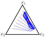
(a) $\eta=0.1$

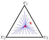
(b) $\eta=4.5$

Figure 3: State trajectories of population $1$ under the logit protocol (12) with $\eta=0.1,4.5$ in the congestion game (2). The payoff vector is determined by (6) subject to a unit time delay ($d=1$). The red circle in both (a) and (b) marks the Nash equilibrium and the red X mark in (b) denotes the unique limit point of all the trajectories.

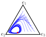
(a) $\eta=0.1$

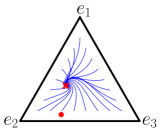
(b) $\eta=0.6$

Figure 4: State trajectories of population $1$ under the logit protocol (12) with $\eta=0.1,0.6$ in the zero-sum game (3). The payoff vector is determined by (9) with $\lambda=1$. The red circle in both (a) and (b) marks the Nash equilibrium and the red X mark in (b) denotes the unique limit point of all the trajectories.

When the payoffs are subject to time delays as in (6) or (9), under existing EDMs, the social state tends to oscillate or converge to equilibrium points that are different from the Nash equilibrium. To illustrate this, using the logit protocol (12) with two different values of $\eta$, Figs. 3 and 4 depict social state trajectories derived in the congestion game (2) where the payoff function is subject to a unit time delay (6) and in the zero-sum game (3) where the payoff vector is defined by the smoothing PDM (9), respectively. We observe that when $\eta$ is small, the resulting social state trajectories oscillate, whereas with a sufficiently large $\eta$, the trajectories converge to an equilibrium point which is located away from the Nash equilibrium of the respective games.

To improve the limitations of existing protocols, we propose a new strategy revision protocol and analyze its convergence properties to rigorously show that the new protocol allows all agents to asymptotically attain the Nash equilibrium even with time delays in payoff mechanisms. We emphasize that such a convergence result for the new model is a distinct contribution. As we illustrated in Figs. 3 and 4, the same convergence cannot be attained with existing models. We formally state the main problem as follows.

 

Problem 1

Design a strategy revision protocol $\mathcal{T}_{ji}^{k}$ and find conditions on the PDM (5) and EDM (11) under which the social state $x(t)$ converges to the Nash equilibrium set $\mathbb{NE}\left(\mathcal{F}\right)$:

$$\lim_{t\to\infty}\inf_{z\in\mathbb{NE}(\mathcal{F})}\|x(t)-z\|_{2}=0.$$

 

III Literature Review

We survey some of the relevant publications in the multi-agent games literature, discuss the effect of time delays in payoff mechanisms, and review works that explore similar ideas of adopting regularization in modeling multi-agent decision making. We then explain how our contributions are distinct.

Multi-agent decision problems formalized by the population games and evolutionary dynamics framework have been one major research theme in control systems and neighboring research communities due to their importance in a wide range of applications [4, 3, 6, 8, 9, 10, 12]. As it has been well-documented in [48, 13], the framework has a long and concrete history of research endeavors in developing Lyapunov stability-based techniques to analyze long-term behavior of decision-making models.

The authors of [46] present pioneering work in generalizing the conventional population games formalism to include dynamic payoff mechanisms, an earlier form of the PDM, and in exploring the use of passivity from dynamical system theory [49] for stability analysis. In subsequent works, such as [50, 51], the PDM formalism has been adopted to model time delays in payoff mechanisms, as in our work, and also to design payoff mechanisms that incentivize decision-making agents to learn and attain the generalized Nash equilibrium, i.e., the Nash equilibrium satisfying given constraints on the agent decision making.

Passivity-based stability analysis presented in [46] unifies notable stability results in the game theory literature, e.g., [44]. Further studies have led to more concrete characterization of stability and development of passivity-based tools for convergence analysis in population games. The tutorial article [37] and its supplementary material [36] detail such formalization and technical discussions on $\delta$-passivity in population games and a wide class of EDMs. The authors of [52] discuss a more general framework – dissipativity tools – for the convergence analysis and explain its importance in analyzing road congestion with mixed autonomy. We also refer the interested reader to [53, 54] for different applications of passivity/dissipativity theory in finite games.

There is a substantial body of literature that investigates the effect of time delays in multi-agent games [18, 19, 20, 21, 22, 23, 24, 25, 26, 27, 28, 29, 30, 31, 32, 33]. These references, as we also illustrated in Figs. 3(a) and 4(a), explain that such time delays result in oscillation of state trajectories. In particular, the references [23, 24, 18, 25, 31, 29, 28] discuss stability of the replicator dynamics in population games defined by affine payoff functions that are subject to time delays. Notably, [25, 26, 30] adopt Hopf bifurcation analysis to rigorously show that oscillation of state trajectories emerges as the time delay increases. Stability and bifurcation analysis on other types of EDMs, such as the best response dynamics and imitation dynamics, in population games with time delays are investigated in [24, 19, 26, 32, 33, 27]. Whereas these works regard the time delays as deterministic parameters in their stability analysis, others [21, 22, 32] study stability of the Nash equilibrium when the time delays are defined by random variables with exponential, uniform, or discrete distributions.

Regularization in designing agent decision-making models has also been explored in multi-agent games. References [55, 56, 57, 58, 54, 53] adopt regularization to design reinforcement learning models and discuss convergence to the Nash equilibrium in finite games. [55] presents an earlier work of so-called exponentially discounted reinforcement learning – later further developed in [58, 54] – and discusses how the regularization improves the convergence of the learning dynamics.

The authors of [56] provide extensive discussions on reinforcement learning models in finite games including the exponentially discounted reinforcement learning model. They rigorously explain convergence properties of regularization-based reinforcement learning models, and also investigate a wide range of control costs to specify the regularization.

[57] explores the use of regularization in population game settings and proposes Riemannian game dynamics, where the regularization is defined by a Riemannian metric such as the Euclidean norm. The authors explain how the Riemannian game dynamics generalize some existing models, such as the replicator dynamics and projection dynamics, and present stability results for their model.

More recent works [54, 53, 37] explain the benefit of the regularization using passivity theory, rigorously showing that the regularization in agent decision-making models enhances the models’ passivity measure. When such decision-making models are interconnected with PDMs, the excess of passivity in the former compensates a shortage of passivity in the latter. Consequently, the feedback interconnection results in the convergence of the social state to an equilibrium state.

Unlike existing studies on the effect of time delays in population games, which focus on identifying technical conditions under which oscillation of state trajectories emerges, we propose a new model that guarantees the convergence of the social state to the Nash equilibrium in a class of contractive population games that are subject to time delays. Although the idea of the regularization and passivity-based analysis have been reported in the multi-agent games literature, all previous results only establish the convergence to the “perturbed” Nash equilibrium. This paper substantially extends our earlier work [50] by generalizing convergence results for the new model to multi-population scenarios and to a more general class of PDMs such as the smoothing PDM.

IV Learning Nash Equilibrium with
Delayed Payoffs

Given $z^{k}=(z_{1}^{k},\cdots,z_{n^{k}}^{k})$ and $\theta^{k}=(\theta_{1}^{k},\cdots,\theta_{n^{k}}^{k})$, both belonging to the interior of the population state space $\mathrm{int}(\mathbb{X}^{k})$, we define the Kullback-Leibler divergence (KLD) as

$$\mathcal{D}(z^{k}\,\|\,\theta^{k})=\textstyle\sum_{i=1}^{n^{k}}z_{i}^{k}\ln\frac{z_{i}^{k}}{\theta_{i}^{k}}.$$ (14)

We compute the gradient of (14) in $\mathbb{X}^{k}$ (with respect to the first argument $z^{k}$) as

$$\nabla\mathcal{D}(z^{k}\,\|\,\theta^{k})=\begin{pmatrix}\ln\frac{z_{1}^{k}}{\theta_{1}^{k}}&\cdots&\ln\frac{z_{n^{k}}^{k}}{\theta_{n^{k}}^{k}}\end{pmatrix}^{T}.$$ (15)

Note that (14) is a convex function of $z^{k}$. For notational convenience, we use $\mathcal{D}(z\,\|\,\theta)=\textstyle\sum_{k=1}^{M}\mathcal{D}(z^{k}\,\|\,\theta^{k})$ and $\nabla\mathcal{D}(z\,\|\,\theta)=(\nabla\mathcal{D}(z^{1}\,\|\,\theta^{1}),\cdots,\nabla\mathcal{D}(z^{M}\,\|\,\theta^{M}))$.

For given $\theta^{k}\in\mathrm{int}(\mathbb{X}^{k})$, using (14), we define the KLD Regularized Learning (KLD-RL) protocol $\mathcal{T}^{\text{\scriptsize KLD-RL}}(\theta^{k},r^{k})=(\mathcal{T}_{1}^{\text{\scriptsize KLD-RL}}(\theta^{k},r^{k}),\cdots,\mathcal{T}_{n^{k}}^{\text{\scriptsize KLD-RL}}(\theta^{k},r^{k}))$ that maximizes a regularized average payoff:

$$\mathcal{T}^{\text{\scriptsize KLD-RL}}(\theta^{k},r^{k})\!=\!\operatorname*{arg\,max}_{z^{k}\in\mathrm{int}(\mathbb{X}^{k})}((z^{k})^{T}r^{k}\!-\!\eta\mathcal{D}(z^{k}\|\theta^{k})),$$ (16)

where $r^{k}\in\mathbb{R}^{n^{k}}$ is the value of population $k$’s payoff vector and $\eta>0$ is a weight on the regularization. Under the protocol, the agents revise their strategies to maximize the cost in (16) that combines the average payoff $(z^{k})^{T}r^{k}$ and the regularization $\mathcal{D}(z^{k}\,\|\,\theta^{k})$ weighted by $\eta$.

By a similar argument as in [34], we can find a unique solution to (16) as

$$\mathcal{T}_{i}^{\text{\scriptsize KLD-RL}}(\theta^{k},r^{k})=\frac{\theta_{i}^{k}\exp(\eta^{-1}r_{i}^{k})}{\sum_{l=1}^{n^{k}}\theta_{l}^{k}\exp(\eta^{-1}r_{l}^{k})}.$$ (17)

One key aspect of the KLD-RL protocol (17) is in using $\theta^{k}$ as a tuning parameter. As a special case, when we assign $\theta^{k}=x^{k}$, (17) becomes the imitative logit protocol [13, Example 5.4.7]. In Section IV-B, we propose an algorithm to compute an appropriate value of $\theta^{k}$ that guarantees the convergence of the social state to the Nash equilibrium set.

To further discuss the effect of $\theta^{k}$ on the agents’ strategy revision, let us consider the following two special cases.

• Case I: If $r_{1}^{k}=\cdots=r_{n^{k}}^{k}$ then

  $$\mathcal{T}_{i}^{\text{\scriptsize KLD-RL}}(\theta^{k},r^{k})=\theta_{i}^{k}.$$

• Case II: If $\theta_{1}^{k}=\cdots=\theta_{n^{k}}^{k}$ then

  $$\mathcal{T}_{i}^{\text{\scriptsize KLD-RL}}(\theta^{k},r^{k})=\frac{\exp(\eta^{-1}r_{i}^{k})}{\sum_{l=1}^{n^{k}}\exp(\eta^{-1}r_{l}^{k})}.$$

From (Case I), we observe that $\theta^{k}$ serves as a bias in the agents’ strategy revision. When the payoffs are identical across all strategies, the agents tend to select a strategy with higher value of $\theta_{i}^{k}$. When there is no bias (Case II), (17) is equivalent to the logit protocol (12).

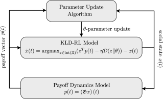
Figure 5: A feedback interconnection illustrating the payoff dynamics model (PDM) and the KLD-RL model along with an algorithm for updating the regularization parameter $\theta$.

To study asymptotic behavior of the EDM (11) defined by KLD-RL protocol (17), we express the state equation of the closed-loop model consisting of (5) and (11) as follows: For $i$ in $\{1,\cdots,n^{k}\}$ and $k$ in $\{1,\cdots,M\}$,

$$\dot{x}_{i}^{k}(t) =\frac{\theta_{i}^{k}\exp(\eta^{-1}p_{i}^{k}(t))}{\sum_{l=1}^{n^{k}}\theta_{l}^{k}\exp(\eta^{-1}p_{l}^{k}(t))}-x_{i}^{k}(t)$$ (18a)

$$p(t) =(\mathfrak{G}x)(t).$$ (18b)

We assume that given an initial condition $(x(0),p(0))\in\mathbb{X}\times\mathbb{R}^{n}$, there is a unique solution to (18). Since $p(t)$ is bounded by Assumption 2-3, social state $x(t)$ belongs to $\mathrm{int}(\mathbb{X})$ for all $t\geq 0$. Fig. 5 illustrates our framework consisting of (18) and a parameter update algorithm for $\theta=(\theta^{1},\cdots,\theta^{M})$.

In Section IV-A, we present preliminary convergence analysis for (18) with parameter $\theta$ fixed. Then, in Section IV-B, we propose a parameter update algorithm that ensures the convergence of the social state $x(t)$ derived by (18) to the Nash equilibrium set.

IV-A Preliminary Convergence Analysis

Our analysis hinges on the passivity technique developed in [46, 36, 37]. We begin by reviewing two notions of passivity – weak $\delta$-antipassivity and $\delta$-passivity – adopted for (5) and (11), respectively. We then establish stability of the closed-loop model (18).

Definition 3 (Weak $\delta$-Antipassivity with Deficit $\nu^{\ast}$ [37])

The PDM (5) is weakly $\delta$-antipassive with deficit $\nu^{\ast}$ if there is a positive and bounded function $\alpha_{x,p}:\mathbb{R}_{+}\to\mathbb{R}_{+}$ for which

$$\alpha_{x,p}(t_{0})\geq\int_{t_{0}}^{t}\left(\dot{x}^{T}(\tau)\dot{p}(\tau)-\nu\,\dot{x}^{T}(\tau)\dot{x}(\tau)\right)\,\mathrm{d}\tau,\\ \forall t\geq t_{0}\geq 0$$ (19)

holds for every social state trajectory $x(t),~{}t\geq 0$ and for every nonnegative constant $\nu>\nu^{\ast}$, where the payoff vector trajectory $p(t),~{}t\geq 0$ is determined by (5) and given ${x(t),~{}t\geq 0}$. The function $\alpha_{x,p}$ satisfies $\lim_{t\to\infty}\alpha_{x,p}(t)=0$ whenever $\lim_{t\to\infty}\|\dot{x}(t)\|_{2}=0$.

The constant $\nu^{\ast}$ is a measure of passivity deficit in (5). Viewing (5) as a dynamical system, according to [49], the function $\alpha_{x,p}$ is an estimate of the stored energy of (5).

In the following lemmas, we establish weak $\delta$-antipassivity of the payoff function with a time delay (6) and the smoothing PDM (9). The proofs of the lemmas are provided in Appendix -A.

Lemma 1

The payoff function with a time delay (6) is weakly $\delta$-antipassive with positive deficit $\nu^{\ast}=B_{D\mathcal{F}}$, where $B_{D\mathcal{F}}$ is the upper bound on $D\mathcal{F}$ as defined in Assumption 1 and $\alpha_{x,p}(t_{0})$ in (19) is defined as

$$\alpha_{x,p}(t_{0})=\frac{B_{D\mathcal{F}}}{2}\int_{t_{0}-d}^{t_{0}}\|\dot{x}(\tau)\|_{2}^{2}\,\mathrm{d}\tau.$$ (20)

By (20), it holds that $\lim_{t\to\infty}\|\dot{x}(t)\|_{2}=0$ implies $\lim_{t\to\infty}\alpha_{x,p}(t)=0$.

Lemma 2

Consider the smoothing PDM (9) where its underlying payoff function is contractive and defined by an affine mapping $\mathcal{F}(x)=Fx+b$. The smoothing PDM is weakly $\delta$-antipassive with positive deficit $\nu^{\ast}$ given by

$$\nu^{\ast}=\frac{1}{4}\|F-F^{T}\|_{2}$$

and $\alpha_{x,p}(t_{0})$ in (19) is defined as

$$\alpha_{x,p}(t_{0})=\sqrt{n}\|p(t_{0})-Fx(t_{0})-b\|_{2},$$ (21)

where $n=\sum_{k=1}^{M}n^{k}$.

Since (9) satisfies Assumption 2-1, $\lim_{t\to\infty}\|\dot{x}(t)\|_{2}=0$ implies $\lim_{t\to\infty}\alpha_{x,p}(t)=0$. If $F$ is symmetric, then $\nu^{\ast}=0$ and the smoothing PDM (9) becomes weakly $\delta$-antipassive without any deficit ($\nu^{\ast}=0$), which coincides with [36, Proposition 7-i)]. Hence, Lemma 2 extends [36, Proposition 7-i)] to the case where $F$ is non-symmetric.

Definition 4 ($\delta$-Passivity with Surplus $\eta^{\ast}$ [37])

The EDM (11) is $\delta$-passive with surplus $\eta^{\ast}$ if there is a continuously differentiable function $\mathcal{S}:\mathbb{X}\times\mathbb{R}^{n}\to\mathbb{R}_{+}$ for which

$$\mathcal{S}\left(x(t),p(t)\right)-\mathcal{S}\left(x(t_{0}),p(t_{0})\right)\leq\\ \int_{t_{0}}^{t}\left(\dot{x}^{T}(\tau)\dot{p}(\tau)-\eta\,\dot{x}^{T}(\tau)\dot{x}(\tau)\right)\,\mathrm{d}\tau,~{}\forall t\geq t_{0}\geq 0$$ (22)

holds for every payoff vector trajectory $p(t),~{}t\geq 0$ and for every nonnegative constant $\eta<\eta^{\ast}$, where the social state trajectory $x(t),~{}t\geq 0$ is determined by (11) and given $p(t),~{}t\geq 0$. We refer to $\mathcal{S}$ as the $\delta$-storage function. We call $\mathcal{S}$ informative if the function satisfies

$$\mathcal{S}\left(z,r\right)\!=\!0\iff\mathcal{V}\left(z,r\right)\!=\!0\iff\nabla_{z}^{T}\mathcal{S}\left(z,r\right)\!\mathcal{V}\left(z,r\right)\!=\!0,$$

where $\mathcal{V}=\left(\mathcal{V}^{1},\cdots,\mathcal{V}^{M}\right)$ denotes the vector field of (11) defining $\dot{x}^{k}(t)=\mathcal{V}^{k}(x^{k}(t),p^{k}(t))$.

The constant $\eta^{\ast}$ is a measure of passivity surplus in (11). Compared to weak $\delta$-antipassivity defined for (5), Definition 4 states a stronger notion of passivity since it requires the existence of the $\delta$-storage function $\mathcal{S}$.

In the following lemma, we establish $\delta$-passivity of the KLD-RL EDM (18a). The proof of the lemma is provided in Appendix -B.

Lemma 3

Given fixed weight $\eta>0$ and regularization parameter $\theta\in\mathrm{int}(\mathbb{X})$, the KLD-RL EDM (18a) is $\delta$-passive with surplus $\eta$ and has an informative $\delta$-storage function $\mathcal{S}_{\theta}:\mathbb{X}\times\mathbb{R}^{n}\to\mathbb{R}_{+}$ expressed as

$$\mathcal{S}_{\theta}(z,r)\!=\!\max_{{\bar{z}}\in\mathrm{int}(\mathbb{X})}(\bar{z}^{T}r\!-\!\eta\mathcal{D}(\bar{z}\|\theta))\!-\!(z^{T}r\!-\!\eta\mathcal{D}(z\|\theta)),$$ (23)

where $z=(z^{1}\!,\!\cdots\!,\!z^{M})$, $r=(r^{1}\!,\!\cdots\!,\!r^{M})$, and $\theta=(\theta^{1}\!,\!\cdots\!,\!\theta^{M})$.

By Assumption 2, (16), and [35, Lemma A.1], the stationary point $(\bar{x},\bar{p})$ of (18) satisfies

$$\max_{z\in\mathbb{X}}(z-\bar{x})^{T}(\mathcal{F}(\bar{x})-\eta\nabla\mathcal{D}(\bar{x}\|\theta))=0$$ (24a)

$$\bar{p}=\mathcal{F}(\bar{x}).$$ (24b)

Following a similar argument as in [35], $\bar{x}$ is the Nash equilibrium of the virtual payoff $\tilde{\mathcal{F}}_{\eta,\theta}$ defined as

$${\tilde{\mathcal{F}}_{\eta,\theta}(z)=\mathcal{F}(z)-\eta\nabla\mathcal{D}(z\,\|\,\theta)}.$$ (25)

The state $\bar{x}$ is often referred to as the perturbed Nash equilibrium of $\mathcal{F}$. Let $\mathbb{PNE}_{\eta,\theta}(\mathcal{F})$ be the set of all perturbed Nash equilibria of $\mathcal{F}$, formally defined as follows.

Definition 5

Given $\eta>0$ and $\theta\in\mathrm{int}\left(\mathbb{X}\right)$, define the set $\mathbb{PNE}_{\eta,\theta}\left(\mathcal{F}\right)$ of the perturbed Nash equilibria of $\mathcal{F}$ as

$$\mathbb{PNE}_{\eta,\theta}\left(\mathcal{F}\right)\!=\!\left\{\bar{z}\!\in\!\mathbb{X}\,\Big{|}\,\left(\bar{z}\!-\!z\right)^{T}\!\tilde{\mathcal{F}}_{\eta,\theta}\left(\bar{z}\right)\!\geq\!0,\forall z\in\mathbb{X}\right\},$$ (26)

where $\tilde{\mathcal{F}}_{\eta,\theta}$ is the virtual payoff (25) associated with $\mathcal{F}$.

Proposition 1

Consider the closed-loop model (18) consisting of the KLD-RL EDM (18a) and PDM (18b). Suppose that (18b) is weakly $\delta$-antipassive with deficit $\nu^{\ast}$ and the weight $\eta$ of (18a) satisfies $\eta>\nu^{\ast}$. The social state $x(t)$ of (18) converges to $\mathbb{PNE}_{\eta,\theta}(\mathcal{F})$:

$$\lim_{t\to\infty}\inf_{z\in\mathbb{PNE}_{\eta,\theta}(\mathcal{F})}\|x(t)-z\|_{2}=0.$$ (27)

Proof:

The proof follows from [36, Lemma 1] provided that $\eta$ is greater than $\nu^{\ast}$. The original statement of [36, Lemma 1] was established for closed-loop models that can be expressed as a finite-dimensional dynamical system. The model (18) may be infinite-dimensional, for instance, when (18b) is the payoff function with a time delay (6). However, given that (18) is well-defined with a unique solution, under Assumption 2, the technical arguments used in the proof of [36, Lemma 1] can be applied to infinite-dimensional models including (6). ∎∎

Proposition 1 implies that if the surplus of passivity in (18a) exceeds the lack of passivity in (18b), the social state, derived by the closed-loop model (18), converges to the perturbed Nash equilibrium set (26). As a consequence, using Lemmas 1 and 2, and Proposition 1, we can establish convergence to the perturbed Nash equilibrium set for the payoff function with a time delay (6) and smoothing PDM (9).

Corollary 1

Suppose the PDM (18b) of the closed-loop model (18) is defined by (6). The social state trajectory, $x(t),~{}t\geq 0$, determined by (18) converges to $\mathbb{PNE}_{\eta,\theta}(\mathcal{F})$ if it holds that $\eta>B_{D\mathcal{F}}$.

Corollary 2

Suppose the PDM (18b) of the closed-loop model (18) is defined by (9) with an affine payoff function $\mathcal{F}(x)=Fx+b$. The social state trajectory, $x(t),~{}t\geq 0$, determined by (18) converges to $\mathbb{PNE}_{\eta,\theta}(\mathcal{F})$ if it holds that $\eta>\frac{1}{4}\left\|F-F^{T}\right\|_{2}$.

IV-B Iterative KLD Regularization and Convergence Guarantee

Suppose the population game $\mathcal{F}$ underlying the PDM (5) has the Nash equilibrium $x^{\tiny\text{NE}}$ belonging to $\mathrm{int}(\mathbb{X})$. If $\theta$ coincides with $x^{\tiny\text{NE}}$, then $\mathbb{PNE}_{\eta,\theta}(\mathcal{F})=\{x^{\tiny\text{NE}}\}$ and under the conditions of Proposition 1, the social state $x(t)$ converges to $x^{\tiny\text{NE}}$. Therefore, to achieve convergence to the Nash equilibrium set, the key requirement is to attain $\theta=x^{\tiny\text{NE}}$. In this section, we discuss the design of a parameter update algorithm that specifies how the agents update $\theta$ to asymptotically attain the Nash equilibrium.

Let the social state $x(t)$ evolve according to (18) and the regularization parameter $\theta$ be iteratively updated at each time instant of a discrete-time sequence $\{t_{l}\}_{l=1}^{\infty}$, determined by a procedure described in Algorithm $1$ below, as $\theta=x(t_{l})\in\mathrm{int}(\mathbb{X})$, i.e., $\theta$ is reset to the current social state $x(t_{l})$ at each time $t_{l}$. Let $\{\theta_{l}\}_{l=1}^{\infty}$ be the resulting sequence of parameter updates. Suppose the following two conditions hold:

$$\max_{z\in\mathbb{X}}(z-\theta_{l+1})^{T}(\mathcal{F}(\theta_{l+1})-\eta\nabla\mathcal{D}(\theta_{l+1}\|\theta_{l}))\\ \leq\frac{\eta}{2}\mathcal{D}(\theta_{l+1}\|\theta_{l})$$ (28a)

$$\lim_{l\to\infty}\mathcal{D}(\theta_{l+1}\|\theta_{l})=0\\ \implies\lim_{l\to\infty}\alpha_{x,p}(t_{l})=0\text{ and }\lim_{l\to\infty}\|p(t_{l})-\mathcal{F}(\theta_{l})\|_{2}\!=\!0,$$ (28b)

where $\alpha_{x,p}$ is the function defined as in (19) for the PDM (18b). According to (24a) and (26), the condition (28a) means that $\theta$ is updated to a new value, i.e., $\theta_{l+1}=x(t_{l+1})$, when the state $x(t_{l+1})$ is sufficiently close to $\mathbb{PNE}_{\eta,\theta_{l}}(\mathcal{F})$. The condition (28b) implies that as the sequence $\{\theta_{l}\}_{l=1}^{\infty}$ converges, the estimated stored energy in the PDM (18b) dissipates and the payoff vector $p(t_{l})$ converges to $\mathcal{F}(\theta_{l})$.

The following lemma states the convergence of the social state $x(t)$ to the Nash equilibrium set $\mathbb{NE}(\mathcal{F})$ if the sequences $\{t_{l}\}_{l=1}^{\infty}$ and $\{\theta_{l}\}_{l=1}^{\infty}$ satisfy (28). The proof of the lemma is given in Appendix -C.

Lemma 4

Consider that the social state $x(t)$ and payoff vector $p(t)$ evolve according to the closed-loop model (18), the PDM (18b) is weakly $\delta$-antipassive with deficit $\nu^{\ast}$, and the regularization parameter $\eta$ of the KLD-RL EDM (18a) satisfies $\eta>\nu^{\ast}$. Suppose the parameter $\theta$ of (18a) is iteratively updated according to $\theta_{l}=x(t_{l}),\,l\in\mathbb{N}$ such that (28) holds, and one of the following two conditions holds.

1. $\mathcal{F}$ is contractive and has a Nash equilibrium in $\mathrm{int}(\mathbb{X})$.

2. $\mathcal{F}$ is strictly contractive.

Then, the state $x(t)$ converges to the Nash equilibrium set:

$$\lim_{t\to\infty}\inf_{z\in\mathbb{NE}(\mathcal{F})}\|x(t)-z\|_{2}=0.$$ (29)

Lemma 4 suggests that if the parameter $\theta$ is updated in a way that the resulting sequence of the parameter updates satisfies (28), the convergence to the Nash equilibrium set is guaranteed. Unlike in Proposition 1, the underlying population game $\mathcal{F}$ needs to be contractive to establish the convergence.

To evaluate (28a) for the parameter update, since the agents may not have access to the quantity $\mathcal{F}(x(t))$, they need to estimate it using the payoff vector $p(t)$. Suppose the estimation error $\|p(t)-\mathcal{F}(x(t))\|_{2}$ is bounded by a function $\beta_{x,p}(t)$, i.e.,

$$\|p(t)-\mathcal{F}(x(t))\|_{2}\leq\beta_{x,p}(t),$$ (30)

for which $\lim_{t\to\infty}\beta_{x,p}(t)=0$ holds whenever the trajectory $x(t),\,t\geq 0$ satisfies $\lim_{t\to\infty}\|\dot{x}(t)\|_{2}=0$. Note that according to Assumption 2-1 such a function $\beta_{x,p}$ always exists. Thus, we derive the following relation.

$$\max_{z\in\mathbb{X}}\left(z-\theta_{l+1}\right)^{T}\left(\mathcal{F}(\theta_{l+1})-\eta\nabla\mathcal{D}\left(\theta_{l+1}\,\|\,\theta_{l}\right)\right)$$

$$\leq\max_{z\in\mathbb{X}}\left(z-\theta_{l+1}\right)^{T}\left(p(t_{l+1})-\eta\nabla\mathcal{D}\left(\theta_{l+1}\,\|\,\theta_{l}\right)\right)$$

$$\qquad\qquad+\max_{z\in\mathbb{X}}\left(z-\theta_{l+1}\right)^{T}\left(\mathcal{F}(\theta_{l+1})-p(t_{l+1})\right)$$

$$\leq\max_{z\in\mathbb{X}}\left(z-\theta_{l+1}\right)^{T}\left(p(t_{l+1})-\eta\nabla\mathcal{D}\left(\theta_{l+1}\,\|\,\theta_{l}\right)\right)$$

$$\qquad\qquad+\sqrt{2M}\|p(t_{l+1})-\mathcal{F}(\theta_{l+1})\|_{2}.$$ (31)

Using (IV-B), we can verify that (28) holds if the parameter is updated as $\theta_{l+1}=x(t_{l+1})$ at each $t_{l+1}$ satisfying

$$\max_{z\in\mathbb{X}}(z-\theta_{l+1})^{T}(p(t_{l+1})-\eta\nabla\mathcal{D}(\theta_{l+1}\|\theta_{l}))\\ +\alpha_{x,p}(t_{l+1})+\sqrt{2M}\beta_{x,p}(t_{l+1})\leq\frac{\eta}{2}\mathcal{D}(\theta_{l+1}\|\theta_{l}).$$ (32)

In what follows, we discuss whether such time instant $t_{l+1}$ always exists. Suppose the parameter $\theta$ is fixed to $\theta_{l}=x(t_{l})$. According to Proposition 1 and the definition of the KLD-RL EDM (18a), the social state $x(t)$ converges to the perturbed Nash equilibrium set $\mathbb{PNE}_{\eta,\theta_{l}}(\mathcal{F})$ which implies

$$\lim_{t\to\infty}\|\dot{x}(t)\|_{2}\to 0$$ (33a)

$$\lim_{t\to\infty}\textstyle\max_{z\in\mathbb{X}}(z\!-\!x(t))^{T}(p(t)\!-\!\eta\nabla\mathcal{D}(x(t)\|\theta_{l}))\to 0.$$ (33b)

Recall that $\lim_{t\to\infty}\|\dot{x}(t)\|_{2}=0$ implies $\lim_{t\to\infty}\alpha_{x,p}(t)=0$ and $\lim_{t\to\infty}\beta_{x,p}(t)=0$. Hence, by (33), the following term vanishes as $t$ tends to infinity.

$$\max_{z\in\mathbb{X}}(z-x(t))^{T}(p(t)-\eta\nabla\mathcal{D}(x(t)\|\theta_{l}))\\ +\alpha_{x,p}(t)+\sqrt{2M}\beta_{x,p}(t).$$ (34)

Consequently, either we can find $t_{l+1}$ satisfying (32) or the state $x(t)$ converges to $\theta_{l}$, i.e., $\lim_{t\to\infty}\mathcal{D}(x(t)\,\|\,\theta_{l})=0$. However, by Proposition 1 and Definition 5, the latter case implies that $\theta_{l}$ needs to be the Nash equilibrium and, hence, the limit point of $x(t)$. In conclusion, for both of the cases, resorting to Lemma 4, the convergence of the social state $x(t)$ to the Nash equilibrium set is guaranteed. In what follows, we only consider the case where the parameter update rule (32) yields an infinite sequence.

Inspired by (32), we propose an algorithm to realize such parameter update for the cases where the PDM (18b) is the payoff function with a time delay (6) or smoothing PDM (9).

  Algorithm $1$: Suppose initial values of the parameter ${\theta\in\mathrm{int}\left(\mathbb{X}\right)}$ and a time instant variable $t_{0}$ are given. Update $\theta$ and $t_{0}$ as $\theta=x(t_{1})$ and $t_{0}=t_{1}$, respectively, if the following conditions hold at any time instant $t_{1}>t_{0}$.

1. Payoff function with a time delay (6):

   $$\max_{z\in\mathbb{X}}\left(z-x(t_{1})\right)^{T}\left(p(t_{1})-\eta\nabla\mathcal{D}\left(x(t_{1})\,\|\,\theta\right)\right)$$

   $$\qquad+\sqrt{2M}B_{D\mathcal{F}}B_{d}\max_{\tau\in[t_{1}-B_{d},t_{1}]}\|\dot{x}(\tau)\|_{2}$$

   $$\leq\frac{\eta}{2}\mathcal{D}\left(x(t_{1})\,\|\,\theta\right)$$ (35)

2. Smoothing PDM (9):

   $$\max_{z\in\mathbb{X}}\left(z-x(t_{1})\right)^{T}\left(p(t_{1})-\eta\nabla\mathcal{D}\left(x(t_{1})\,\|\,\theta\right)\right)$$

   $$\qquad+\sqrt{2M}\Big{(}\left(\left\|p(\gamma t_{1})\right\|_{2}+B_{\mathcal{F}}\right)\exp({-\lambda\left(1-\gamma\right)t_{1}})$$

   $$\qquad+B_{D\mathcal{F}}\int_{\gamma t_{1}}^{t_{1}}\exp({-\lambda(t_{1}-\tau)})\left\|\dot{x}(\tau)\right\|_{2}\,\mathrm{d}\tau\Big{)}$$

   $$\leq\frac{\eta}{2}\mathcal{D}\left(x(t_{1})\,\|\,\theta\right)$$ (36)

where $x(t)$ is the social state at time instant $t$, $\gamma$ is any fixed real number in $(0,1)$, and $\dot{x}(\tau)$ can be computed using (18a).

 

To realize Algorithm 1, the agents only need to know the upper bounds $B_{d},B_{D\mathcal{F}}$ on $d,D\mathcal{F}$ for (6), or the bounds $B_{\mathcal{F}},B_{D\mathcal{F}}$ on $\mathcal{F},D\mathcal{F}$ for (9). The motivation behind adopting the algorithm is analogous to iterative regularization techniques that have been frequently used in optimization and machine learning methods to avoid issues with over-fitting or fluctuation, especially when cost functions are noisy [59]. Similarly, in our multi-agent learning problem, Algorithm 1 prevents the state trajectory from exhibiting oscillation and ensures the convergence to the Nash equilibrium set.

Leveraging Lemmas 1-4, in the following theorems, we state convergence results for the closed-loop model (18) when $\theta$ of (18a) is updated according to Algorithm 1 and (18b) is a payoff function with a time delay (6) (Theorem 1) or smoothing PDM (9) (Theorem 2). The proofs of the theorems are provided in Appendix -D.

Theorem 1

Suppose that the social state $x(t)$ and payoff vector $p(t)$ are derived by the closed-loop model (18), where the PDM (18b) is a payoff function with a time delay (6). If $\mathcal{F}$ satisfies one of the conditions (C1) or (C2) stated in Lemma 4, $\eta>B_{D\mathcal{F}}$ holds, and the parameter $\theta$ is iteratively updated according to (1), then the state $x(t)$ converges to the Nash equilibrium set.

Theorem 2

Suppose that the social state $x(t)$ and payoff vector $p(t)$ are derived by the closed-loop model (18), where the PDM (18b) is a smoothing PDM (9). If $\mathcal{F}$ satisfies one of the conditions (C1) or (C2) stated in Lemma 4, $\eta>\frac{1}{4}\|F-F^{T}\|_{2}$ holds, and the parameter $\theta$ is iteratively updated according to (2), then the state $x(t)$ converges to the Nash equilibrium set.

V Simulations with Numerical Examples

We use Examples 1 and 2 to illustrate our main results. To this end, we evaluate the social state trajectory of the closed-loop model (18) when the PDM (18b) is defined by (i) the payoff function with a time delay (6) with the payoff function $\mathcal{F}$ defined as in (2) and (ii) the smoothing PDM (9) with $\mathcal{F}$ defined as in (3).

V-A Convergence and Performance Improvements

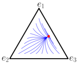
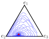
Figure 6: State trajectories of population 1 derived by the closed-loop model (18). The PDM (18b) is defined by (a) the payoff function with a time delay with $\mathcal{F}$ given by (2) and (b) the smoothing PDM (9) with $\mathcal{F}$ defined by (3). The parameter $\eta$ of the EDM (18a) is selected as $\eta=4.5$ for (a) and $\eta=0.6$ for (b). The red circle in (a) and (b) marks the Nash equilibrium of each game.

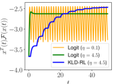
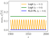
Figure 7: (a) Average payoff $x^{T}(t)\mathcal{F}(x(t))$ of the entire society in the congestion game and (b) maximum gain $\max_{i\in\{1,2,3\}}\mathcal{F}_{i}^{2}(x(t))$ of population 2 (the opponent of population 1) in the zero-sum game for the logit protocol ($\eta=0.1,4.5$) and KLD-RL protocol ($\eta=4.5$).

V-A1 Congestion Population Game with Time Delay

We illustrate our main results using the congestion population game (2) with a unit time delay ($d=1$). For (18a), we set $\eta=4.5$ to ensure that $\eta>B_{D\mathcal{F}}$, where $B_{D\mathcal{F}}$ is chosen to be the $2$-norm of the payoff matrix (2), and update the parameter $\theta$ using (1) in Algorithm 1. For simplicity, we assign $B_{d}=d$.

Fig. 6 illustrates that resulting social state trajectories converge to the unique Nash equilibrium of (2). Recall that for the logit protocol case, as depicted in Fig. 3, the social state trajectories either exhibit oscillation around the Nash equilibrium (when $\eta$ is small) or converge to a stationary point located away from the Nash equilibrium (when $\eta$ is large).

To assess the efficacy of the KLD-RL model for agents to learn an effective strategy profile in the congestion game, we compare the average payoff $x^{T}(t)\mathcal{F}(x(t))$ using the social state $x(t)$ derived by the logit protocol (12) with $\eta=0.1,4.5$ and the KLD-RL protocol (17) with ${\eta=4.5}$. As shown in Fig. 7, only the social state trajectory determined by (17) converges and asymptotically attains the largest average payoff, which is approximately $-2.44$.

V-A2 Zero-sum Game with Smoothing PDM

We iterate the simulations using the smoothing PDM (9) defined by the zero-sum game (3). We assign $\lambda=1$ for (9), set $\eta=0.6$ for (18a) to ensure that $\eta>\frac{1}{4}\|F-F^{T}\|_{2}$ holds, where $F$ is the matrix given as in (3), and update the parameter $\theta$ using (2) in Algorithm 1 with $\gamma=0.1$.

As illustrated in Fig. 6, resulting social state trajectories converge to the unique Nash equilibrium of (3). This can be compared to the time-delay case considered in Section V-A1, shown in Fig. 4, where the state trajectories derived by the logit protocol either exhibit oscillation around the Nash equilibrium (when $\eta$ is small) or converge to a stationary point located away from the Nash equilibrium (when $\eta$ is large).

To assess the efficacy of the KLD-RL model for each population to learn an effective strategy profile in the zero-sum game, we evaluate the maximum gain $\max_{i\in\{1,2,3\}}\mathcal{F}_{i}^{2}(x(t))$ of population 2 (the opponent of population 1), using the social state $x(t)$ that results from the logit protocol (12) with $\eta=0.1,0.6$ and the KLD-RL protocol (17) with ${\eta=0.6}$. As shown in Fig. 7, only the social state trajectory determined by (17) converges to the strategy profile at which the maximum gain of population 2 is minimized.

V-B Selection of regularization weight $\eta$

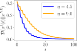
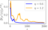
Figure 8: Graphs of the KL divergence $\mathcal{D}(x^{1}(t)\|x^{\text{\scriptsize NE}})$ between the state of population 1 and the Nash equilibrium in (a) the congestion game and (b) the zero-sum game.

As stated in Theorems 1 and 2, a proper selection of $\eta$ in (18a) is critical. In particular, for (6) and (9), $\eta$ needs to be larger than $B_{D\mathcal{F}}$ and $\frac{1}{4}\|F-F^{T}\|_{2}$, respectively, to ensure convergence to the Nash equilibrium set. In practice, unless the payoff function $\mathcal{F}$ is available, the agents need to estimate upper bounds on $B_{D\mathcal{F}}$ and $\frac{1}{4}\|F-F^{T}\|_{2}$ and select $\eta$ to be larger than these estimates. When these estimates are conservative, the agents will select unnecessarily large $\eta$.

Recall that $\eta$ determines the weight on the regularization in the KLD-RL protocol (16): Smaller $\eta$ means that the regularization has little effect on the strategy revision and the agents tend to select strategies that increase the average payoff. Hence, assigning smaller $\eta$ would imply faster convergence to the Nash equilibrium set. We verify such observation using simulations. Fig. 8 depicts the simulation results with two different values of $\eta$ in each of the two PDM cases we considered in Section V-A. In both cases, when $\eta$ is small, we can observe that the social state converges to the unique Nash equilibrium of each game faster than when $\eta$ is large. In conclusion, for achieving faster convergence to the Nash equilibrium set, the agents need to assign a small value to $\eta$ satisfying the inequality requirement $\eta>\nu^{\ast}$ for the convergence as we discussed in Lemma 4, and this will require computing an accurate estimate of $\nu^{\ast}$.

VI Extensions

We explain potential extensions of the problem formulation investigated in this paper and discuss convergence results we can establish. These results can be proved with similar arguments as in this paper, so we omit details for brevity.

VI-A Multiple Time Delays

In (6), we consider that the payoff function is subject to a single time delay. In practical scenarios, for instance in the congestion game, the time delay would vary across available strategies. As an immediate extension of (6), we can consider the payoff function with multiple time delays formulated as

$$p(t)=\textstyle\sum_{i=1}^{N_{d}}\mathcal{F}_{i}(x-d_{i}),$$ (37)

where the payoff function $\mathcal{F}$ of an underlying population game can be recovered by setting $d_{i}=0,~{}\forall i\in\{1,\cdots,N_{d}\}$, i.e., $\mathcal{F}(x)=\sum_{i=1}^{N_{d}}\mathcal{F}_{i}(x)$. Similar analysis established for the single time-delay case can be applied for (37).

VI-B Mixed Population Scenario

The parameter update described in Algorithm 1 is an essential step to guarantee the convergence to the Nash equilibrium set. However, such update requires coordination among all agents in every population, which can be hard to achieve. For instance, the agents in each population $k$ need to agree on a single time instant $t_{1}$ to update the parameter $\theta^{k}$ to $x^{k}(t_{1})$.

As an extension, below we consider a scenario where select populations in the society adopt the KLD-RL protocol (17) along with Algorithm 1 for the parameter update and all other populations choose the logit protocol (12). We discuss how the convergence results of Lemma 4 can be generalized to such scenario. For a concise presentation, we consider a two-population formulation where the agents in each population adopt the following protocols for their strategy revision:

$$\dot{x}_{i}^{1}(t) =\frac{\theta_{i}\exp(\eta^{-1}p_{i}^{1}(t))}{\sum_{l=1}^{n^{1}}\theta_{l}\exp(\eta^{-1}p_{l}^{1}(t))}-x_{i}^{1}(t),~{}i=1,\cdots,n^{1}$$ (38a)

$$\dot{x}_{j}^{2}(t) =\frac{\exp(\eta^{-1}p_{j}^{2}(t))}{\sum_{l=1}^{n^{2}}\exp(\eta^{-1}p_{l}^{2}(t))}-x_{j}^{2}(t),~{}j=1,\cdots,n^{2}$$ (38b)

where the payoff vector $p(t)=(p^{1}(t),p^{2}(t))$ is determined by the PDM (5).

Imposing the same requirements as in Lemma 4, we can establish that the social state $x(t)=(x^{1}(t),x^{2}(t))$ of (38) converges to the set of equilibrium points $\bar{x}=(\bar{x}^{1},\bar{x}^{2})$ satisfying

$$\bar{x}^{1} \in\operatorname*{arg\,max}_{z^{1}\in\mathbb{X}^{1}}(z^{1})^{T}\mathcal{F}^{1}(\bar{x}^{1},\bar{x}^{2})$$ (39a)

$$\bar{x}^{2} \in\operatorname*{arg\,max}_{z^{2}\in\mathbb{X}^{2}}\left((z^{2})^{T}\mathcal{F}^{2}(\bar{x}^{1},\bar{x}^{2})-\eta h(z^{2})\right)$$ (39b)

where $\mathcal{F}=(\mathcal{F}^{1},\mathcal{F}^{2})$ is the payoff function of an underlying population game. According to (39), at the equilibrium, the agents in population 1 select the strategy profile that is the best response to the population 2’s strategy profile $\bar{x}^{2}$; whereas those in population 2 adopt the strategy profile that is the perturbed best response to population 1’s strategy profile $\bar{x}^{1}$.

VI-C Distributed Parameter Update

We consider the scenario where the state and payoffs associated with a population are private information and the agents in each population do not want to share it with others outside the population as exposing such private information would make vulnerable their decision making, e.g., using the information, agents of an adversarial population could revise their strategies to deliberately diminish payoffs of the exposed population. However, notice that to validate the conditions (1) and (2) of Algorithm 1, every population in the society needs to assess the states and payoffs of all other populations. In the following, we discuss how Algorithm 1 can be revised to address the privacy issue.

We proceed with stating the conditions (1) and (2) for each population $k$, respectively, as follows:

$$\max_{z^{k}\in\mathbb{X}^{k}}(z^{k}-x^{k}(t_{1}))^{T}(p^{k}(t_{1})-\eta\nabla\mathcal{D}(x^{k}(t_{1})\|\theta^{k}))$$

$$\qquad+\sqrt{2M}B_{D\mathcal{F}}B_{d}\max_{\tau\in[t_{1}-B_{d},t_{1}]}\|\dot{x}^{k}(\tau)\|_{2}$$

$$\leq\frac{\eta}{2}\mathcal{D}(x^{k}(t_{1})\|\theta^{k})$$ (40)

and

$$\max_{z^{k}\in\mathbb{X}^{k}}(z^{k}-x^{k}(t_{1}))^{T}\left(p^{k}(t_{1})-\eta\nabla\mathcal{D}\left(x^{k}(t_{1})\,\|\,\theta^{k}\right)\right)$$

$$\quad+\sqrt{2M}\Big{(}\Big{(}\|p^{k}(\gamma t_{1})\|_{2}+\frac{B_{\mathcal{F}}}{M}\Big{)}\exp(-\lambda(1-\gamma)t_{1})$$

$$\quad+B_{D\mathcal{F}}\int_{\gamma t_{1}}^{t_{1}}\exp(-\lambda(t_{1}-\tau))\|\dot{x}^{k}(\tau)\|_{2}\,\mathrm{d}\tau\Big{)}$$

$$\leq\frac{\eta}{2}\mathcal{D}(x^{k}(t_{1})\,\|\,\theta^{k}).$$ (41)

Using the facts that $\|\dot{x}(\tau)\|_{2}\leq\sum_{k=1}^{M}\|\dot{x}^{k}(\tau)\|_{2}$ and $\|p(\gamma t_{1})\|_{2}\leq\sum_{k=1}^{M}\|p^{k}(\gamma t_{1})\|_{2}$, we can validate (1) and (2) if (VI-C) and (VI-C) hold for all $k$ in $\{1,\cdots,M\}$, respectively.

Consequently, each population $k$ only needs to inform all other populations whether the conditions (VI-C) and (VI-C) are satisfied at each time $t$, without sharing other information including its parameter $\theta^{k}$, population state $x^{k}(t)$, and payoff vector $p^{k}(t)$. If all populations agree on a single time instant $t_{1}$, e.g. using a consensus algorithm [60], at which (VI-C) and (VI-C) hold for all $k$ in $\{1,\cdots,M\}$, then each population $k$ can update the parameter $\theta^{k}$ to its state $x^{k}(t_{1})$ at time $t_{1}$.

VII Conclusions

We studied a multi-agent decision problem in population games in which decision-making agents repeatedly revise their strategy choices based on time-delayed payoffs. We illustrated that under the existing logit model, the agents’ strategy revision process may oscillate or converge to the perturbed Nash equilibrium. To address such limitation of existing models, we proposed the KLD-RL model and rigorously prove that the new model allows the agents to asymptotically attain the Nash equilibrium despite the time delays.

We illustrated our main results using simulations in the two-population congestion game and zero-sum game, and compared the simulation outcomes with those derived by the logit model. In particular, the outcomes suggest that when the payoffs are subject to time delays, the KLD-RL model is advantageous in learning effective strategy profiles in both games, whereas the state trajectories determined by the logit model either oscillate or converge to a stationary point representing non-effective strategy profiles.

As future directions, we plan to investigate the scenario where the agents’ decision making is subject to constrained inter-agent communication and explore how the KLD-RL model can be adopted to learn effective strategies under limited information exchange among the agents. Also, we are interested in applying the KLD-RL model in relevant engineering applications such as multi-vehicle route planning, multi-robot task allocation, and security in power systems, where time delays are inherent in underlying dynamic processes and communication systems.

-A Proofs of Lemmas 1 and 2

-A1 Proof of Lemma 1

According to Assumption 1, we have that

$$\tilde{z}^{T}D\mathcal{F}^{T}(z)D\mathcal{F}(z)\tilde{z}\leq B_{D\mathcal{F}}^{2}\tilde{z}^{T}\tilde{z},~{}\forall z\in\mathbb{X},\tilde{z}\in T\mathbb{X}$$ (42)

where $D\mathcal{F}$ is the differential map of $\mathcal{F}$. Using (42), we can derive the following relations.

$$\int_{t_{0}}^{t}\dot{x}^{T}(\tau)\dot{p}(\tau)\,\mathrm{d}\tau$$

$$=\int_{t_{0}}^{t}\dot{x}^{T}(\tau)D\mathcal{F}(x(\tau-d))\dot{x}(\tau-d)\,\mathrm{d}\tau$$

$$\overset{(i)}{\leq}\frac{B_{D\mathcal{F}}}{2}\int_{t_{0}}^{t}\dot{x}^{T}(\tau)\dot{x}(\tau)\,\mathrm{d}\tau$$

$$\qquad+\frac{1}{2B_{D\mathcal{F}}}\int_{t_{0}}^{t}\dot{x}^{T}(\tau-d)D\mathcal{F}^{T}(x(\tau-d))$$

$$\qquad\qquad\qquad\qquad\qquad\qquad\times D\mathcal{F}(x(\tau-d))\dot{x}(\tau-d)\,\mathrm{d}\tau$$

$$\overset{(ii)}{\leq}\frac{B_{D\mathcal{F}}}{2}\!\int_{t_{0}}^{t}\dot{x}^{T}\!(\tau)\dot{x}(\tau)\,\mathrm{d}\tau\!+\!\frac{B_{D\mathcal{F}}}{2}\!\int_{t_{0}}^{t}\dot{x}^{T}\!(\tau\!-\!d)\dot{x}(\tau\!-\!d)\,\mathrm{d}\tau$$

$$\leq B_{D\mathcal{F}}\int_{t_{0}}^{t}\dot{x}^{T}(\tau)\dot{x}(\tau)\,\mathrm{d}\tau+\frac{B_{D\mathcal{F}}}{2}\int_{t_{0}-d}^{t_{0}}\dot{x}^{T}(\tau)\dot{x}(\tau)\,\mathrm{d}\tau$$ (43)

To show that $(i)$ and $(ii)$ hold, we use (42) and the following fact:

$$\dot{x}^{T}(\tau)D\mathcal{F}(x(\tau-d))\dot{x}(\tau-d)\leq\frac{B_{D\mathcal{F}}}{2}\dot{x}^{T}(\tau)\dot{x}(\tau)\\ +\frac{1}{2B_{D\mathcal{F}}}\dot{x}^{T}(\tau-d)D\mathcal{F}^{T}(x(\tau-d))D\mathcal{F}(x(\tau-d))\dot{x}(\tau-d).$$

Therefore, by defining $\alpha_{x,p}(t_{0})=\frac{B_{D\mathcal{F}}}{2}\int_{t_{0}-d}^{t_{0}}\|\dot{x}(\tau)\|_{2}^{2}\,\mathrm{d}\tau$, we conclude that (6) is weakly $\delta$-antipassive with deficit $B_{D\mathcal{F}}$. ∎

-A2 Proof of Lemma 2

We proceed by following similar steps as in the proof of [36, Proposition 7]. Using the linear superposition principle, we express the solution of (9) as

$$p(t) =\exp(-\lambda(t-t_{0}))p(t_{0})$$

$$\qquad+\lambda\int_{t_{0}}^{t}\exp(-\lambda(t-\tau))\left(Fx(t_{0})+b\right)\,\mathrm{d}\tau$$

$$\qquad+\lambda\int_{t_{0}}^{t}\exp(-\lambda(t-\tau))F\left(x(\tau)-x(t_{0})\right)\,\mathrm{d}\tau$$

$$=\underbrace{\exp(-\lambda(t-t_{0}))(p(t_{0})-Fx(t_{0})-b)+Fx(t_{0})+b}_{=p^{h}(t)}$$

$$\qquad+\underbrace{\lambda\int_{t_{0}}^{t}\exp(-\lambda(t-\tau))F\left(x(\tau)-x(t_{0})\right)\,\mathrm{d}\tau}_{=p^{f}(t)}.$$

Note that

$$\int_{t_{0}}^{t}\dot{x}^{T}(\tau)\dot{p}^{h}(\tau)\,\mathrm{d}\tau$$

$$=\lambda\int_{t_{0}}^{t}\dot{x}^{T}(\tau)\exp(-\lambda(\tau-t_{0}))(Fx(t_{0})+b-p(t_{0}))\,\mathrm{d}\tau$$

$$\leq\sqrt{n}\|Fx(t_{0})+b-p(t_{0})\|_{2}.$$ (44)

To derive the inequality, we use the fact that the strategy revision protocol $\mathcal{T}_{ij}^{k}(x^{k}(t),p^{k}(t))$ in (11) is a probability distribution, and it holds that

$$0\leq\mathcal{T}_{ij}^{k}(x^{k}(t),p^{k}(t))\leq 1$$ (45a)

$$\textstyle\sum_{j=1}^{n^{k}}\mathcal{T}_{ij}^{k}(x^{k}(t),p^{k}(t))=1.$$ (45b)

Using (45), from (11), we can derive $|\dot{x}_{i}^{k}(t)|\leq 1$, and hence $\|\dot{x}(t)\|_{2}\leq\sqrt{n}$ for all $t\geq 0$, where $n=\sum_{k=1}^{M}n^{k}$.

Let us define

$$\alpha_{x,p}(t_{0})=\sqrt{n}\left\|Fx(t_{0})+b-p(t_{0})\right\|_{2}.$$

Now we proceed to show that

$$\int_{t_{0}}^{t}\dot{x}^{T}(\tau)\dot{p}^{f}(\tau)\,\mathrm{d}\tau\leq\int_{t_{0}}^{t}\nu^{\ast}\dot{x}^{T}(\tau)\dot{x}(\tau)\,\mathrm{d}\tau$$ (46)

with $\nu^{\ast}$ given in the statement of Lemma 2. By noting that the transfer function from $\dot{x}$ to $\dot{p}^{f}$ is $\frac{\lambda}{\lambda+s}F$ and using Parseval’s theorem, (46) holds if the following inequality is satisfied:

$$z^{H}\left(\frac{\lambda}{\lambda+j\omega}F+\frac{\lambda}{\lambda-j\omega}F^{T}\right)z\leq 2\nu^{\ast}z^{H}z,\\ \forall\omega\in\mathbb{R},z\in T\mathbb{C}^{n},$$ (47)

where $T\mathbb{C}^{n}$ is the tangent space of the $n$-dimensional complex space $\mathbb{C}^{n}$ defined as

$$T\mathbb{C}^{n}=\big{\{}(z^{1},\cdots,z^{M})\in\mathbb{C}^{n^{1}}\times\cdots\times\mathbb{C}^{n^{M}}\,\big{|}\,\\ \textstyle\sum_{i=1}^{n^{k}}z_{i}^{k}=0,~{}\forall k\in\{1,\cdots,M\}\big{\}}.$$

Note that (47) can be re-written as

$$\lambda^{2}z^{H}\left(F+F^{T}\right)z-j\lambda\omega z^{H}\left(F-F^{T}\right)z\\ \leq 2\nu^{\ast}\left(\lambda^{2}+\omega^{2}\right)z^{H}z.$$ (48)

By representing $F$ as the sum of its symmetric and skew-symmetric parts, $F=F_{\tiny\text{sym}}+F_{\tiny\text{skew}}$, and the complex variable $z$ as $z=z_{R}+jz_{I}$ with $z_{R},z_{I}\in\mathbb{R}^{n}$, we can rewrite (48) into

$$\lambda^{2}\left(z_{R}^{T}F_{\text{sym}}z_{R}+z_{I}^{T}F_{\text{sym}}z_{I}\right)-2\lambda\omega z_{I}^{T}F_{\text{skew}}z_{R}\\ \leq\nu^{\ast}\left(\lambda^{2}+\omega^{2}\right)(z_{R}^{T}z_{R}+z_{I}^{T}z_{I}).$$ (49)

Since $F$ is contractive, $F_{\text{sym}}$ is a negative-semidefinite matrix in $T\mathbb{X}$ and for the inequality (49) to hold, it suffices to show that

$$-\frac{2\lambda\omega}{\nu^{\ast}\left(\lambda^{2}+\omega^{2}\right)}z_{I}^{T}F_{\text{skew}}z_{R}\leq z_{R}^{T}z_{R}+z_{I}^{T}z_{I}.$$ (50)

Note that

$$z_{R}^{T}z_{R}+z_{I}^{T}z_{I}+\frac{2\lambda\omega}{\nu^{\ast}\left(\lambda^{2}+\omega^{2}\right)}z_{I}^{T}F_{\text{skew}}z_{R}$$

$$=\!\left(z_{R}\!-\!\frac{\lambda\omega}{\nu^{\ast}\!\left(\lambda^{2}\!+\!\omega^{2}\right)}F_{\text{skew}}z_{I}\right)^{T}\!\left(z_{R}\!-\!\frac{\lambda\omega}{\nu^{\ast}\!\left(\lambda^{2}\!+\!\omega^{2}\right)}F_{\text{skew}}z_{I}\right)$$

$$\qquad-z_{I}^{T}F_{\text{skew}}^{T}F_{\text{skew}}z_{I}\left(\frac{\lambda\omega}{\nu^{\ast}\left(\lambda^{2}+\omega^{2}\right)}\right)^{2}+z_{I}^{T}z_{I}$$

$$\geq z_{I}^{T}\left(I-\frac{1}{4{\nu^{\ast}}^{2}}F_{\text{skew}}^{T}F_{\text{skew}}\right)z_{I}$$

Hence, if $\nu^{\ast}$ satisfies $\nu^{\ast}\geq\frac{1}{2}\left\|F_{\text{skew}}\right\|_{2}$ then the inequality (50) holds. In conjunction with (-A2), we conclude that

$$\int_{t_{0}}^{t}\left(\dot{x}^{T}(\tau)\dot{p}(\tau)-\nu\dot{x}^{T}(\tau)\dot{x}(\tau)\right)\,\mathrm{d}\tau\leq\alpha_{x,p}(t_{0})$$ (51)

holds for any $\nu\geq\frac{1}{4}\left\|F-F^{T}\right\|_{2}$ and $\alpha_{x,p}(t_{0})=\sqrt{n}\left\|Fx(t_{0})+b-p(t_{0})\right\|_{2}$. ∎

-B Proof of Lemma 3

We begin by recalling the perturbed best response EDM [36, Section VIII] whose state equation is given as

$$\dot{x}^{k}(t)=\operatorname*{arg\,max}_{z^{k}\in\mathrm{int}(\mathbb{X}^{k})}((z^{k})^{T}p^{k}(t)-\mathcal{Q}^{k}(z^{k}))-x^{k}(t),$$ (52)

where $\mathcal{Q}^{k}:\mathrm{int}(\mathbb{X}^{k})\to\mathbb{R}$ is so-called the admissible perturbation that satisfies the following two conditions:

$$\lim_{z^{k}\to\mathrm{bd}(\mathbb{X}^{k})}\|\nabla\mathcal{Q}^{k}(z^{k})\|_{2}=\infty$$

$$(\tilde{z}^{k})^{T}\nabla^{2}\mathcal{Q}^{k}(z^{k})\tilde{z}^{k}\!\geq\!\eta(\tilde{z}^{k})^{T}\tilde{z}^{k},~{}\forall z^{k}\!\in\!\mathrm{int}(\mathbb{X}^{k}),\tilde{z}^{k}\!\in\!T\mathbb{X}^{k},$$

where $\nabla\mathcal{Q}^{k}$ and $\nabla^{2}\mathcal{Q}^{k}$ are the gradient and Laplacian of $\mathcal{Q}^{k}$ in $\mathrm{int}(\mathbb{X}^{k})$, respectively, and $\mathrm{bd}(\mathbb{X}^{k})$ is the boundary of $\mathbb{X}^{k}$ defined as $\mathrm{bd}(\mathbb{X}^{k})=\mathbb{X}^{k}\setminus\mathrm{int}(\mathbb{X}^{k})$. With the parameter $\theta^{k}\in\mathrm{int}(\mathbb{X}^{k})$ fixed, we can validate that the KLD-RL EDM (18a) is a perturbed best response EDM with ${\mathcal{Q}^{k}(z^{k})=\eta\mathcal{D}(z^{k}\,\|\,\theta^{k})}$. Hence, using [36, Proposition 5], we assert that (18a) is $\delta$-passivity with surplus $\eta$ and (23) is its informative $\delta$-storage function. ∎

-C Proof of Lemma 4

Recall that $\{t_{l}\}_{l=1}^{\infty}$ is the sequence of time instants at which the parameter $\theta$ of the KLD-RL EDM is updated and $\{\theta_{l}\}_{l=1}^{\infty}$ is the sequence of resulting parameters, i.e., $\theta_{l}=x(t_{l}),~{}\forall l\in\mathbb{N}$, satisfying (28). We provide a two-part proof: In the first part, we establish that $\{\theta_{l}\}_{l=1}^{\infty}$ converges to $\mathbb{NE}(\mathcal{F})$. Then, using the result from the first part, we show that the social state $x(t)$ converges to $\mathbb{NE}(\mathcal{F})$.

Part I

Let $x^{\text{\scriptsize NE}}$ be an arbitrary Nash equilibrium in $\mathbb{NE}(\mathcal{F})$. By Definition 1, it holds that

$$(x^{\text{\scriptsize NE}}-z)^{T}\mathcal{F}(x^{\text{\scriptsize NE}})\geq 0,~{}\forall z\in\mathbb{X}.$$ (53)

Note that (28a) suggests that $\{\theta_{l}\}_{l=1}^{\infty}$ satisfies

$$(\theta_{l+1}-x^{\text{\scriptsize NE}})^{T}\left(\mathcal{F}(\theta_{l+1})-\eta\nabla\mathcal{D}(\theta_{l+1}\,\|\,\theta_{l})\right)\\ \geq-\frac{\eta}{2}\mathcal{D}(\theta_{l+1}\,\|\,\theta_{l}).$$ (54)

Since $\mathcal{F}$ is a contractive population game under both conditions (C1) or (C2) stated in the lemma, using (4) and (53), it holds that

$$(\theta_{l+1}\!-\!x^{\text{\scriptsize NE}})^{T}\mathcal{F}(\theta_{l+1})\!\leq\!(\theta_{l+1}\!-\!x^{\text{\scriptsize NE}})^{T}\mathcal{F}(x^{\text{\scriptsize NE}})\!\leq\!0.$$ (55)

Also, using (14) and (15), we can establish

$$(x^{\text{\scriptsize NE}})^{T}\nabla\mathcal{D}(\theta_{l+1}\|\theta_{l})=\mathcal{D}(x^{\text{\scriptsize NE}}\|\theta_{l})-\mathcal{D}(x^{\text{\scriptsize NE}}\|\theta_{l+1}).$$ (56)

Using (54)-(56), we can derive

$$0 \geq(\theta_{l+1}-x^{\text{\scriptsize NE}})^{T}\nabla\mathcal{D}(\theta_{l+1}\,\|\,\theta_{l})-\frac{1}{2}\mathcal{D}(\theta_{l+1}\|\theta_{l})$$

$$=\mathcal{D}(\theta_{l+1}\|\theta_{l})\!-\!\mathcal{D}(x^{\text{\scriptsize NE}}\|\theta_{l})\!+\!\mathcal{D}(x^{\text{\scriptsize NE}}\|\theta_{l+1})\!-\!\frac{1}{2}\mathcal{D}(\theta_{l+1}\|\theta_{l})$$

and hence we conclude

$$\mathcal{D}(x^{\text{\scriptsize NE}}\|\theta_{l+1})\leq\mathcal{D}(x^{\text{\scriptsize NE}}\|\theta_{l})-\frac{1}{2}\mathcal{D}(\theta_{l+1}\|\theta_{l}).$$ (57)

From (57), we can infer that $\{\mathcal{D}(x^{\text{\scriptsize NE}}\|\theta_{l})\}_{l=1}^{\infty}$ is a monotonically decreasing sequence, and since every $\mathcal{D}(x^{\text{\scriptsize NE}}\|\theta_{l})$ is nonnegative, it holds that $\lim_{l\to\infty}\mathcal{D}(\theta_{l+1}\|\theta_{l})=0$. Therefore, according to (28a), we have that

$$\lim_{l\to\infty}\max_{z\in\mathbb{X}}(z-\theta_{l+1})^{T}(\mathcal{F}(\theta_{l+1})-\eta\nabla\mathcal{D}(\theta_{l+1}\|\theta_{l}))=0.$$ (58)

Let $\theta_{l}=(\theta_{l}^{1},\cdots,\theta_{l}^{M})\in\mathbb{X}$ and $\theta_{l}^{k}=(\theta_{l,1}^{k},\cdots,\theta_{l,n^{k}}^{k})\in\mathbb{X}^{k}$. Since $\mathcal{D}(\theta_{l+1}\|\theta_{l})$ converges to zero as $l$ tends to infinity, $\lim_{l\to\infty}\theta_{l,i}^{k}=0$ implies $\lim_{l\to\infty}\theta_{l+1,i}^{k}=0$. Also if $\theta_{l}$ converges to $\bar{\theta}$, then so does $\theta_{l+1}$.

To complete the proof of Part I, it is sufficient to show that when a subsequence $\{\theta_{l_{m}}\}_{m=1}^{\infty}$ converges to $\bar{\theta}\in\mathbb{X}$, it holds that $\bar{\theta}\in\mathbb{NE}(\mathcal{F})$. From (58), we can derive

$$\max_{z\in\mathbb{X}_{\bar{\theta}}}(z-\bar{\theta})^{T}\mathcal{F}(\bar{\theta})$$

$$=\!\lim_{m\to\infty}\max_{z\in\mathbb{X}_{\bar{\theta}}}(z\!-\!\theta_{l_{m}\!+\!1})^{T}\!(\mathcal{F}(\theta_{l_{m}\!+\!1})\!-\!\eta\nabla\mathcal{D}(\theta_{l_{m}\!+\!1}\|\theta_{l_{m}}))$$

$$\leq\!\lim_{m\to\infty}\max_{z\in\mathbb{X}}(z\!-\!\theta_{l_{m}\!+\!1})^{T}\!(\mathcal{F}(\theta_{l_{m}\!+\!1})\!-\!\eta\nabla\mathcal{D}(\theta_{l_{m}\!+\!1}\|\theta_{l_{m}}))\!=\!0,$$ (59)

where $\mathbb{X}_{\bar{\theta}}$ is a subset of $\mathbb{X}$ given by $\mathbb{X}_{\bar{\theta}}=\{x\in\mathbb{X}\,|\,x_{i}^{k}=0\text{ if }\bar{\theta}_{i}^{k}=0\}$. Note that every Nash equilibrium $x^{\text{NE}}$ of $\mathcal{F}$ belongs to $\mathbb{X}_{\bar{\theta}}$; otherwise there is $x^{\text{NE}}\in\mathbb{NE}(\mathcal{F})$ for which $\lim_{m\to\infty}\mathcal{D}(x^{\text{NE}}\|\theta_{l_{m}})=\infty$, which contradicts the fact that $\{\mathcal{D}(x^{\text{NE}}\|\theta_{l})\}_{l=1}^{\infty}$ is a decreasing sequence. Then, the following inequalities hold:

$$(x^{\text{NE}}-\bar{\theta})^{T}\mathcal{F}(\bar{\theta})\leq 0$$ (60a)

$$(x^{\text{NE}}-\bar{\theta})^{T}\mathcal{F}(x^{\text{NE}})\geq 0.$$ (60b)

If the condition (C1) of the lemma holds, then $\mathbb{X}_{\bar{\theta}}=\mathbb{X}$ and, hence, by (-C), $\bar{\theta}$ is a Nash equilibrium. In addition, if the condition (C2) holds, then using (60) and since $\mathcal{F}$ is strictly contractive, we can establish $(x^{\text{NE}}-\bar{\theta})^{T}(\mathcal{F}(x^{\text{NE}})-\mathcal{F}(\bar{\theta}))=0$ which implies $\bar{\theta}=x^{\text{NE}}$. Hence, every limit point $\bar{\theta}$ of $\{\theta_{l}\}_{l=1}^{\infty}$ belongs to $\mathbb{NE}(\mathcal{F})$. Therefore, we conclude that the sequence $\left\{\theta_{l}\right\}_{l=1}^{\infty}$ converges to the Nash equilibrium set $\mathbb{NE}(\mathcal{F})$.

Part II

Let $\alpha_{x,p}$ be the upper bound of the inequality (19). By (28b), it holds that $\lim_{l\to\infty}\alpha_{x,p}(t_{l})=0$. Also, let $\mathcal{S}_{\theta_{l}}(x(t),p(t))$ be the informative $\delta$-storage function of the KLD-RL EDM, defined as in (23), over the time interval $t\in[t_{l},t_{l+1})$. Using (19) and (22), we can derive

$$\mathcal{S}_{\theta_{l}}(x(t),p(t))\!\leq\!\mathcal{S}_{\theta_{l}}(x(t_{l}),p(t_{l}))\!+\!\alpha_{x,p}(t_{l}),~{}\forall t\!\in\![t_{l},t_{l+1}).$$ (61)

Given that $\theta_{l}=x(t_{l})$, the term $\mathcal{S}_{\theta_{l}}(x(t_{l}),p(t_{l}))$ can be rewritten as

$$\mathcal{S}_{\theta_{l}}(x(t_{l}),p(t_{l}))$$

$$=\max_{\bar{z}\in\mathrm{int}(\mathbb{X})}(\bar{z}^{T}p(t_{l})-\eta\mathcal{D}(\bar{z}\,\|\,\theta_{l}))-\theta_{l}^{T}p(t_{l})$$

$$=\eta\textstyle\sum_{k=1}^{M}\ln\left(\textstyle\sum_{s=1}^{n^{k}}\theta_{l,s}^{k}\exp(\eta^{-1}p_{s}^{k}(t_{l}))\right)-\theta_{l}^{T}p(t_{l}),$$ (62)

where we use (16) and (17) to derive the last equality. By (28b) and (-C), we observe that for any convergent subsequence $\{\theta_{l_{m}}\}_{m=1}^{\infty}$ of $\{\theta_{l}\}_{l=1}^{\infty}$ with its limit point $\bar{\theta}$ in $\mathbb{NE}(\mathcal{F})$, it holds that

$$\lim_{m\to\infty}\ln\left(\textstyle\sum_{s=1}^{n^{k}}\theta_{l_{m},s}^{k}\exp(\eta^{-1}p_{s}^{k}(t_{l_{m}}))\right)\\ =\eta^{-1}\max_{j\in\{1\leq s\leq n^{k}\,|\,\bar{\theta}_{s}^{k}>0\}}\mathcal{F}_{j}^{k}(\bar{\theta})$$

from which we can establish that

$$\lim_{l\to\infty}\mathcal{S}_{\theta_{l}}(x(t_{l}),p(t_{l}))=0.$$ (63)

Consequently, for any $\epsilon>0$, we can find a positive integer $L$ for which

$$\mathcal{S}_{\theta_{l}}(x(t),p(t))\leq\epsilon,~{}\forall t\in[t_{l},t_{l+1})$$ (64)

holds for all $l\geq L$.

Note that $\mathcal{D}(z\,\|\,\theta_{l})$ is a strongly convex function of $z$, i.e., $\nabla^{2}\mathcal{D}(z\,\|\,\theta_{l})\geq I$. According to the analysis used in [34, Theorem 2.1],

$$\eta\tilde{z}^{T}\nabla\mathcal{D}(y\,\|\,\theta_{l})=\tilde{z}^{T}r\\ \iff y=\operatorname*{arg\,max}_{z\in\mathrm{int}(\mathbb{X})}(z^{T}r-\eta\mathcal{D}(z\,\|\,\theta_{l}))$$ (65)

holds for all $r\in\mathbb{R}^{n}$, $y\in\mathrm{int}(\mathbb{X})$, and $\tilde{z}\in T\mathbb{X}$. Let $y(t)=\operatorname*{arg\,max}_{z\in\mathrm{int}(\mathbb{X})}(z^{T}p(t)-\eta\mathcal{D}(z\,\|\,\theta_{l}))$, then we can derive

$$\mathcal{S}_{\theta_{l}}(x(t),p(t))=\eta(y(t)-x(t))^{T}\nabla\mathcal{D}(y(t)\,\|\,\theta_{l})\\ -\eta(\mathcal{D}(y(t)\,\|\,\theta_{l})-\mathcal{D}(x(t)\,\|\,\theta_{l}))\geq\frac{\eta}{2}\|y(t)-x(t)\|_{2}^{2},$$ (66)

where to establish the inequality, we use the strong convexity of $\mathcal{D}(z\,\|\,\theta_{l})$. In conjunction with (64) and (66), by the definition of the KLD-RL protocol (16), we conclude that $\lim_{t\to\infty}\|\dot{x}(t)\|_{2}=0$.

We complete the proof by showing that the social state $x(t)$ converges to $\mathbb{NE}(\mathcal{F})$. By contradiction, suppose that there is a sequence $\{\tau_{m}\}_{m=1}^{\infty}$ of time instants for which $\left\{x(\tau_{m})\right\}_{m=1}^{\infty}$ converges to $\bar{x}$, where $\bar{x}$ does not belong to $\mathbb{NE}(\mathcal{F})$. Let $\{[t_{l_{m}},t_{l_{m}+1})\}_{m=1}^{\infty}\subseteq\{[t_{l},t_{l+1})\}_{l=1}^{\infty}$ be the collection of time intervals for which $\tau_{m}\in[t_{l_{m}},t_{l_{m}+1})$ holds for all $m\in\mathbb{N}$. By Assumption 2-1, (61), and (63), we have that

$$\max_{\bar{z}\in\mathbb{X}}\left(\bar{z}^{T}\mathcal{F}(\bar{x})\!-\!\eta\mathcal{D}(\bar{z}\|\bar{\theta})\right)\!-\!\left(\bar{x}^{T}\mathcal{F}(\bar{x})\!-\!\eta\mathcal{D}(\bar{x}\|\bar{\theta})\right)\!=\!0,$$ (67)

where $\bar{\theta}$ is a limit point of the subsequence $\left\{\theta_{l_{m}}\right\}_{m=1}^{\infty}$ of $\left\{\theta_{l}\right\}_{l=1}^{\infty}$. By (67) and the facts that $\bar{\theta}$ belongs to $\mathbb{NE}(\mathcal{F})$ and $\mathcal{F}$ is contractive, we can derive

$$\eta\mathcal{D}(\bar{x}\,\|\,\bar{\theta})\leq(\bar{x}-\bar{\theta})^{T}\mathcal{F}(\bar{x})\leq(\bar{x}-\bar{\theta})^{T}\mathcal{F}(\bar{\theta})\leq 0,$$

which yields that $\bar{x}=\bar{\theta}$. This contradicts our hypothesis that $\bar{x}$ does not belong to $\mathbb{NE}(\mathcal{F})$. ∎

-D Proofs of Theorems 1 and 2

-D1 Proof of Theorem 1

According to Lemmas 1-4, it suffices to show that (1) of Algorithm 1 implies (28). Let $\{\theta_{l}\}_{l=1}^{\infty}$ be a sequence of parameter updates determined by (1) of Algorithm 1. Note that

$$\max_{z\in\mathbb{X}}(z-\theta_{l+1})^{T}(\mathcal{F}(\theta_{l+1})-\eta\nabla\mathcal{D}(\theta_{l+1}\|\theta_{l}))$$

$$\leq\max_{z\in\mathbb{X}}(z-\theta_{l+1})^{T}(p(t_{l+1}))-\eta\nabla\mathcal{D}(\theta_{l+1}\|\theta_{l}))$$

$$\qquad+\sqrt{2M}\|p(t_{l+1})-\mathcal{F}(\theta_{l+1})\|_{2}\,.$$ (68)

We can establish a bound on $\|p(t_{l+1})-\mathcal{F}(\theta_{l+1})\|_{2}$ as follows:

$$\|p(t_{l+1})-\mathcal{F}(\theta_{l+1})\|_{2}$$

$$=\|\mathcal{F}(x(t_{l+1}-d))-\mathcal{F}(x(t_{l+1}))\|_{2}$$

$$\leq\max_{z\in\mathbb{X}}\|D\mathcal{F}(z)\|_{2}\|x(t_{l+1}-d)-x(t_{l+1})\|_{2}$$

$$\leq B_{D\mathcal{F}}B_{d}\max_{\tau\in[t_{l+1}-B_{d},t_{l+1}]}\|\dot{x}(\tau)\|_{2}$$ (69)

where $B_{d}$ upper bounds $d$ in (6) and $B_{D\mathcal{F}}$ upper bounds $D\mathcal{F}$. Hence, by (-D1) and (-D1), (1) implies (28a). To establish (28b), suppose $\lim_{l\to\infty}\mathcal{D}(\theta_{l+1}\|\theta_{l})=0$. Using (1), we can derive $\lim_{l\to\infty}\max_{\tau\in[t_{l+1}-B_{d},t_{l+1}]}\|\dot{x}(\tau)\|_{2}=0$ from which we conclude that

$$\lim_{l\to\infty}\|p(t_{l})-\mathcal{F}(x(t_{l}))\|_{2}=0$$

$$\lim_{l\to\infty}\alpha_{x,p}(t_{l})=\lim_{l\to\infty}\frac{B_{D\mathcal{F}}}{2}\int_{t_{l}-d}^{t_{l}}\left\|\dot{x}(\tau)\right\|_{2}\,\mathrm{d}\tau=0.$$

This completes the proof. ∎

-D2 Proof of Theorem 2

Similar to the proof of Theorem 1, we show that (2) of Algorithm 1 implies (28). We begin with establishing a bound on $\|p(t_{l+1})-\mathcal{F}(x(t_{l+1}))\|_{2}$. Consider the following differential equation:

$$\frac{\mathrm{d}}{\mathrm{d}t}(p(t)-\mathcal{F}(x(t)))\\ =-\lambda(p(t)-\mathcal{F}(x(t)))-D\mathcal{F}(x(t))\dot{x}(t).$$ (70)

For any $t_{0}<t_{l+1}$, a solution to the equation at $t=t_{l+1}$ can be computed as

$$p(t_{l+1})-\mathcal{F}(x(t_{l+1}))$$

$$=(p(t_{0})-\mathcal{F}(x(t_{0})))\exp(-\lambda(t_{l+1}-t_{0}))$$

$$\qquad-\int_{t_{0}}^{t_{l+1}}\exp({-\lambda(t_{l+1}-\tau)})D\mathcal{F}(x(\tau))\dot{x}(\tau)\,\mathrm{d}\tau.$$ (71)

By assigning $t_{0}=\gamma t_{l+1}$ with $\gamma\in(0,1)$, we obtain

$$\|p(t_{l+1})-\mathcal{F}(x(t_{l+1}))\|_{2}$$

$$\leq(\|p(\gamma t_{l+1})\|_{2}+B_{\mathcal{F}})\exp(-\lambda(1-\gamma)t_{l+1})$$

$$\qquad+B_{D\mathcal{F}}\int_{\gamma t_{l+1}}^{t_{l+1}}\exp({-\lambda(t_{l+1}-\tau)})\|\dot{x}(\tau)\|_{2}\,\mathrm{d}\tau.$$ (72)

Hence, in conjunction with (-D1) and (-D2), we observe that (2) implies (28a). To establish (28b), using (2) and (-D2), if $\lim_{l\to\infty}\mathcal{D}(\theta_{l+1}\|\theta_{l})=0$ then it holds that

$$\lim_{l\to\infty}\left\|p(t_{l})-\mathcal{F}\left(x(t_{l})\right)\right\|_{2}=0,$$ (73)

which implies

$$\lim_{l\to\infty}\alpha_{x,p}(t_{l})=\lim_{l\to\infty}\sqrt{n}\left\|p(t_{l})-Fx(t_{l})-b\right\|_{2}=0,$$ (74)

where we use $\mathcal{F}(x)=Fx+b$. This completes the proof. ∎

Shinkyu Park (M’16) received the B.S. degree from Kyungpook National University, Daegu, Korea, in 2006, the M.S. degree from Seoul National University, Seoul, Korea, in 2008, and the Ph.D. degree from the University of Maryland, College Park, MD, USA, in 2015, all in electrical engineering. From 2016 to 2019, he was a Postdoctoral Associate at Massachusetts Institute of Technology, and from 2019 to 2021, he was appointed as an Associate Research Scholar at Princeton University. He is currently the Assistant Professor of Electrical and Computer Engineering at King Abdullah University of Science and Technology (KAUST). His research interests are in robotics, multi-agent decision-making, feedback control theory, and game theory.

Naomi Ehrich Leonard (F’07) received the B.S.E. degree in mechanical engineering from Princeton University, Princeton, NJ, USA, in 1985, and the M.S.and Ph.D. degrees in electrical engineering from the University of Maryland, College Park, MD, USA, in 1991 and 1994, respectively. From 1985 to 1989, she was an Engineer in the electric power industry. She is currently the Edwin S. Wilsey Professor of Mechanical and Aerospace Engineering and Associated Faculty of the Program in Applied and Computational Mathematics at Princeton University. She is also Founding Editor of the Annual Review of Control, Robotics, and Autonomous Systems. Her research and teaching are in control and dynamical systems with current interests in networked multi-agent systems, robotics, collective animal behavior, and social decision-making.

References

- [1] D. Liu, A. Hafid, and L. Khoukhi, “Population game based energy and time aware task offloading for large amounts of competing users,” in 2018 IEEE Global Comm. Conf. (GLOBECOM), 2018, pp. 1–6.
- [2] S. Moon, H. Kim, and Y. Yi, “Brute: Energy-efficient user association in cellular networks from population game perspective,” IEEE Trans. Wireless Communications, vol. 15, no. 1, pp. 663–675, 2016.
- [3] S. Park, Y. D. Zhong, and N. E. Leonard, “Multi-robot task allocation games in dynamically changing environments,” in 2021 IEEE International Conference on Robotics and Automation (ICRA), 2021, pp. 8678–8684.
- [4] P. Srikantha and D. Kundur, “Resilient distributed real-time demand response via population games,” IEEE Transactions on Smart Grid, vol. 8, no. 6, pp. 2532–2543, 2017.
- [5] D. Lee and D. Kundur, “An evolutionary game approach to predict demand response from real-time pricing,” in 2015 IEEE Electrical Power and Energy Conference (EPEC), 2015, pp. 197–202.
- [6] E. Ramírez-Llanos and N. Quijano, “A population dynamics approach for the water distribution problem,” International Journal of Control, vol. 83, no. 9, pp. 1947–1964, 2010.
- [7] A. Pashaie, L. Pavel, and C. J. Damaren, “A population game approach for dynamic resource allocation problems,” International Journal of Control, vol. 90, no. 9, pp. 1957–1972, 2017.
- [8] G. Obando, A. Pantoja, and N. Quijano, “Building temperature control based on population dynamics,” IEEE Transactions on Control Systems Technology, vol. 22, no. 1, pp. 404–412, 2014.
- [9] H. Tembine, E. Altman, R. El-Azouzi, and Y. Hayel, “Evolutionary games in wireless networks,” IEEE Trans. Systems, Man, and Cybernetics, Part B (Cybernetics), vol. 40, no. 3, pp. 634–646, 2010.
- [10] J. Martinez-Piazuelo, N. Quijano, and C. Ocampo-Martinez, “Decentralized charging coordination of electric vehicles using multi-population games,” in 2020 59th IEEE Conference on Decision and Control (CDC), 2020, pp. 506–511.
- [11] N. Quijano, C. Ocampo-Martinez, J. Barreiro-Gomez, G. Obando, A. Pantoja, and E. Mojica-Nava, “The role of population games and evolutionary dynamics in distributed control systems: The advantages of evolutionary game theory,” IEEE Control Systems Magazine, vol. 37, no. 1, pp. 70–97, 2017.
- [12] N. Li and J. R. Marden, “Designing games for distributed optimization,” IEEE Journal of Selected Topics in Signal Processing, vol. 7, no. 2, pp. 230–242, 2013.
- [13] W. H. Sandholm, Population Games and Evolutionary Dynamics. MIT Press, 2011.
- [14] P. Kollock, “Social dilemmas: The anatomy of cooperation,” Annual Review of Sociology, vol. 24, no. 1, pp. 183–214, 1998.
- [15] S. Park, A. Bizyaeva, M. Kawakatsu, A. Franci, and N. E. Leonard, “Tuning cooperative behavior in games with nonlinear opinion dynamics,” IEEE Control Systems Letters, vol. 6, pp. 2030–2035, 2022.
- [16] M. J. Smith, “The stability of a dynamic model of traffic assignment—an application of a method of Lyapunov,” Transportation Science, vol. 18, no. 3, pp. 245–252, 1984.
- [17] I. Menache and A. Ozdaglar, “Network Games: Theory, Models, and Dynamics,” Synthesis Lectures on Communication Networks, vol. 4, no. 1, pp. 1–159, Mar. 2011, publisher: Morgan & Claypool Publishers.
- [18] J. Alboszta and J. Mie¸kisz, “Stability of evolutionarily stable strategies in discrete replicator dynamics with time delay,” Journal of Theoretical Biology, vol. 231, no. 2, pp. 175 – 179, 2004.
- [19] H. Oaku, “Evolution with delay,” The Japanese Economic Review, vol. 53, pp. 114–133, 2002.
- [20] M. Bodnar, J. Miȩkisz, and R. Vardanyan, “Three-player games with strategy-dependent time delays,” Dynamic Games and Applications, vol. 10, pp. 664–675, 2020.
- [21] N. Ben-Khalifa, R. El-Azouzi, and Y. Hayel, “Discrete and continuous distributed delays in replicator dynamics,” Dynamic Games and Applications, vol. 8, pp. 713–732, 2018.
- [22] R. Iijima, “On delayed discrete evolutionary dynamics,” Journal of Theoretical Biology, vol. 300, pp. 1 – 6, 2012.
- [23] T. Yi and W. Zuwang, “Effect of time delay and evolutionarily stable strategy,” J. Theoretical Biology, vol. 187, no. 1, pp. 111 – 116, 1997.
- [24] H. Tembine, E. Altman, R. El-Azouzi, and Y. Hayel, “Bio-inspired delayed evolutionary game dynamics with networking applications,” Telecommunication Systems, vol. 47, pp. 137–152, 2011.
- [25] E. Wesson and R. Rand, “Hopf bifurcations in delayed rock–paper–scissors replicator dynamics,” Dynamic Games and Applications, vol. 6, pp. 139–156, 2016.
- [26] S. Mittal, A. Mukhopadhyay, and S. Chakraborty, “Evolutionary dynamics of the delayed replicator-mutator equation: Limit cycle and cooperation,” Phys. Rev. E, vol. 101, p. 042410, Apr 2020.
- [27] S.-C. Wang, J.-R. Yu, S. Kurokawa, and Y. Tao, “Imitation dynamics with time delay,” J. Theoretical Biology, vol. 420, pp. 8 – 11, 2017.
- [28] N. B. Khalifa, R. El-Azouzi, and Y. Hayel, “Delayed evolutionary game dynamics with non-uniform interactions in two communities,” in 53rd IEEE Conf. Decision and Control, 2014, pp. 3809–3814.
- [29] G. Obando, J. I. Poveda, and N. Quijano, “Replicator dynamics under perturbations and time delays,” Mathematics of Control, Signals, and Systems, vol. 28, no. 20, 2016.
- [30] N. Sîrghi and M. Neamţu, “Dynamics of deterministic and stochastic evolutionary games with multiple delays,” International Journal of Bifurcation and Chaos, vol. 23, no. 07, p. 1350122, 2013.
- [31] H. Tembine, E. Altman, and R. El-Azouzi, “Asymmetric delay in evolutionary games,” in Proceedings of the 2nd International Conference on Performance Evaluation Methodologies and Tools, ser. ValueTools ’07. ICST (Institute for Computer Sciences, Social-Informatics and Telecommunications Engineering), 2007.
- [32] W. Hu, G. Zhang, and H. Tian, “The stability of imitation dynamics with discrete distributed delays,” Physica A: Statistical Mechanics and its Applications, vol. 521, pp. 218 – 224, 2019.
- [33] R. Iijima, “Heterogeneous information lags and evolutionary stability,” Mathematical Social Sciences, vol. 61, no. 2, pp. 83–85, March 2011.
- [34] J. Hofbauer and W. H. Sandholm, “On the global convergence of stochastic fictitious play,” Econometrica, vol. 70, no. 6, pp. 2265–2294, 2002.
- [35] ——, “Evolution in games with randomly disturbed payoffs,” Journal of Economic Theory, vol. 132, no. 1, pp. 47 – 69, 2007.
- [36] S. Park, N. C. Martins, and J. S. Shamma, “Payoff dynamics model and evolutionary dynamics model: Feedback and convergence to equilibria (arxiv:1903.02018),” arXiv.org, March 2019.
- [37] ——, “From population games to payoff dynamics models: A passivity-based approach,” in 2019 IEEE 58th Conference on Decision and Control (CDC), 2019, pp. 6584–6601.
- [38] D. Monderer and L. S. Shapley, “Potential games,” Games and Economic Behavior, vol. 14, no. 1, pp. 124 – 143, 1996.
- [39] W. H. Sandholm, “Potential games with continuous player sets,” Journal of Economic Theory, vol. 97, no. 1, pp. 81 – 108, 2001.
- [40] ——, “Chapter 13: Population games and deterministic evolutionary dynamics,” ser. Handbook of Game Theory with Economic Applications, H. P. Young and S. Zamir, Eds. Elsevier, 2015, vol. 4, pp. 703–778.
- [41] S. Omidshafiei, C. Papadimitriou, G. Piliouras, K. Tuyls, M. Rowland, J.-B. Lespiau, W. M. Czarnecki, M. Lanctot, J. Perolat, and R. Munos, “-rank: Multi-agent evaluation by evolution,” Scientific Reports, vol. 9, no. 1, p. 9937, Jul 2019.
- [42] Y.-P. Li, S.-Y. Tan, Y. Deng, and J. Wu, “Attacker-defender game from a network science perspective,” Chaos: An Interdisciplinary Journal of Nonlinear Science, vol. 28, no. 5, p. 051102, 2018.
- [43] T. Alpcan, Game Theory for Security. London: Springer London, 2015, pp. 495–499.
- [44] J. Hofbauer and W. H. Sandholm, “Stable games and their dynamics,” Journal of Economic Theory, vol. 144, no. 4, pp. 1665–1693.4, July 2009.
- [45] A. van der Schaft, L2-Gain and Passivity Techniques in Nonlinear Control, 3rd ed. Springer Publishing Company, Incorporated, 2016.
- [46] M. J. Fox and J. S. Shamma, “Population games, stable games, and passivity,” Games, vol. 4, pp. 561–583, Oct. 2013.
- [47] S. Park, J. S. Shamma, and N. C. Martins, “Passivity and evolutionary game dynamics,” in 2018 IEEE Conference on Decision and Control (CDC), 2018, pp. 3553–3560.
- [48] J. Hofbauer and K. Sigmund, Evolutionary Games and Population Dynamics. Cambridge University Press, 1998.
- [49] J. C. Willems, “Dissipative dynamical systems part I: General theory,” Arch. Ration. Mech. Anal., vol. 45, no. 5, pp. 321–351, Jan. 1972.
- [50] S. Park and N. E. Leonard, “KL divergence regularized learning model for multi-agent decision making,” in 2021 American Control Conference (ACC), 2021, pp. 4509–4514.
- [51] J. Martinez-Piazuelo, N. Quijano, and C. Ocampo-Martinez, “A payoff dynamics model for generalized nash equilibrium seeking in population games,” Automatica, vol. 140, p. 110227, 2022.
- [52] M. Arcak and N. C. Martins, “Dissipativity tools for convergence to nash equilibria in population games,” IEEE Transactions on Control of Network Systems, vol. 8, no. 1, pp. 39–50, 2021.
- [53] L. Pavel, “Dissipativity theory in game theory: On the role of dissipativity and passivity in nash equilibrium seeking,” IEEE Control Systems Magazine, vol. 42, no. 3, pp. 150–164, 2022.
- [54] B. Gao and L. Pavel, “On passivity, reinforcement learning and higher-order learning in multi-agent finite games,” IEEE Transactions on Automatic Control, pp. 1–1, 2020.
- [55] D. S. Leslie and E. J. Collins, “Individual Q-learning in normal form games,” SIAM Journal on Control and Optimization, vol. 44, no. 2, 2005.
- [56] P. Mertikopoulos and W. H. Sandholm, “Learning in games via reinforcement and regularization,” Mathematics of Operations Research, vol. 41, no. 4, pp. 1297–1324, 2016.
- [57] ——, “Riemannian game dynamics,” Journal of Economic Theory, vol. 177, pp. 315–364, 2018.
- [58] P. Coucheney, B. Gaujal, and P. Mertikopoulos, “Penalty-regulated dynamics and robust learning procedures in games,” Mathematics of Operations Research, vol. 40, no. 3, pp. 611–633, 2015.
- [59] E. Alpaydin, Introduction to Machine Learning, 2nd ed. The MIT Press, 2010.
- [60] R. Olfati-Saber, J. A. Fax, and R. M. Murray, “Consensus and cooperation in networked multi-agent systems,” Proceedings of the IEEE, vol. 95, no. 1, pp. 215–233, 2007.