Hybrid and Oriented Harmonic Potentials for Safe Task Execution
in Unknown Environment

Abstract

Harmonic potentials provide globally convergent potential fields that are provably free of local minima. Due to its analytical format, it is particularly suitable for generating safe and reliable robot navigation policies. However, for complex environments that consist of a large number of overlapping non-sphere obstacles, the computation of associated transformation functions can be tedious. This becomes more apparent when: (i) the workspace is initially unknown and the underlying potential fields are updated constantly as the robot explores it; (ii) the high-level mission consists of sequential navigation tasks among numerous regions, requiring the robot to switch between different potentials. Thus, this work proposes an efficient and automated scheme to construct harmonic potentials incrementally online as guided by the task automaton. A novel two-layer harmonic tree (HT) structure is introduced that facilitates the hybrid combination of oriented search algorithms for task planning and harmonic-based navigation controllers for non-holonomic robots. Both layers are adapted efficiently and jointly during online execution to reflect the actual feasibility and cost of navigation within the updated workspace. Global safety and convergence are ensured both for the high-level task plan and the low-level robot trajectory. Known issues such as oscillation or long-detours for purely potential-based methods and sharp-turns or high computation complexity for purely search-based methods are prevented. Extensive numerical simulation and hardware experiments are conducted against several strong baselines.

1 Introduction

Autonomous robots can replace humans to operate and accomplish complex missions in hazardous environments. However, it is a demanding engineering task to ensure both the safety and efficiency during execution, especially when the environment is only partially known. First, the control strategy that drives the robot from an initial state to the goal state while staying within the allowed workspace (see e.g., Karaman & Frazzoli (2011); LaValle (2006); Koditschek (1987); Khatib (1999)), should be reactive to the newly-discovered obstacles online. Second, the planning method that decomposes and schedules sub-tasks (see e.g., Ghallab et al. (2004); Fainekos et al. (2009)) should be adaptive to the actual feasibility and cost of sub-tasks given the updated environment. Existing work often ignores the close dependency of these two modules and treats them separately, which can lead to inefficient or even unsafe executions, as also motivated in Garrett et al. (2021); Kim et al. (2022). How to construct a fully integrated task and motion planning scheme with provable safety and efficiency guarantee within unknown environments still remains challenging, see Loizou & Rimon (2022); Rousseas et al. (2022b).

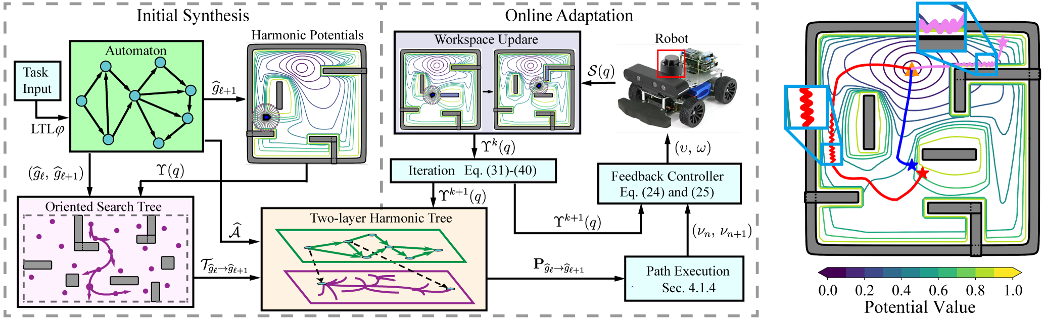
Figure 1: Left: Illustration of the proposed framework, which consists of the initial synthesis, the online adaption of the task plan and harmonic potentials, and the hybrid execution. Right: Oscillations and long detours might occur via classic navigation functions as shown in the red, violet and blue trajectories.

1.1 Related Work

As the most relevant to this work, the method of artificial potential fields from Khatib (1986); Warren (1989); Panagou (2014); Rousseas et al. (2022a) introduces an intuitive yet powerful framework for tackling the safety and convergence property during navigation. The main idea is to introduce attractive potentials to the goal state and repulsive potentials from obstacles and the workspace boundary. However, naive design of these potentials would introduce undesired local minima, where the combined forces are zero and thus prevents further progress. Navigation functions (NF) pioneered by Koditschek (1987) provably guarantee that such minima are saddle points and more importantly of measure zero. Although the underlying static workspace could be as general as forest of stars, some key design parameters require fine-tuning for the safety and convergence properties to hold. The work in Fan et al. (2022) employs the conformal transformations to map the multiply-connected workspaces to a sphere world without any tuning parameter, which however requires a numerical solution of continuous integrals. Moreover, harmonic potentials proposed in Kim & Khosla (1992); Loizou (2011, 2017); Vlantis et al. (2018) alleviate such limitations by introducing a novel transformation scheme from obstacle-cluttered environments to point worlds, while retaining these properties. Furthermore, recent work in  Rousseas et al. (2021, 2022b, 2022a) resolves the need for a diffeomorphic mapping onto sphere disks, by adopting a wider set of basis functions for workspace boundaries. Nevertheless, such methods require solving numerous complex parametric optimizations, instead of an analytic solution. Lastly, despite of their global convergence guarantee, there are several notable limitations as illustrated in Fig. 1: (i) oscillations or jitters may appear especially when the trajectory slides along the boundary of obstacles or crosses narrow passages; (ii) drastically different trajectories may develop within the same potential field when the initial pose is changed slightly; (iii) the resulting trajectory is far from the optimal one in terms of trajectory length or control efforts; (iv) the final orientation at the goal pose can not be controlled freely.

Moreover, sampling-based search methods, such as RRT^⋆ in Karaman & Frazzoli (2011), PRM in Hsu et al. (2006), FMT^⋆ in Janson et al. (2015), have become the dominant paradigm to tackle high-dimensional motion planning problems, especially for systems under geometric and dynamic constraints. However, one potential limiting factor is the high computational complexity due to the collision checking process between sampled states and the excessive sampling to reach convergence. Since artificial potential fields are analytical and can ensure safety and convergence as described earlier, it make sense to combine these two paradigms. Some recent work can be found in this direction: vector fields are used in Ko et al. (2013) to bias the branching of search trees, thus improving the efficiency of sampling and reducing the number of iterations; similar ideas are adopted in Qureshi & Ayaz (2016); Tahir et al. (2018) as the potential-function-based RRT^⋆, by designing directional samples as induced by the underlying potential fields. Higher efficiency and faster convergence are shown compared with the raw RRT^⋆ algorithm. However, these methods mostly focus on static environments for simple navigation tasks, where the planning is performed offline and neither the potential fields nor the search structure are adapted during execution.

When a robot is deployed in a partially-unknown environment, an online approach is required such that the underlying trajectory adapts to real-time measurements of the actual workspace such as new obstacles. For instances, a fully automated tuning mechanism for navigation functions is presented in Filippidis & Kyriakopoulos (2011), while the notion of dynamic windows is proposed in Ogren & Leonard (2005) to handle dynamic environment. Moreover, the harmonic potentials-based methods are developed further in Rousseas et al. (2022b) for unknown environments, where the weights over harmonic basis are optimized online. A similar formulation is adopted in Loizou & Rimon (2022) where the parameters in the harmonic potentials are adjusted online to ensure safety and global convergence. Furthermore, a semantic perceptual feedback me-thod is introduced in Vasilopoulos et al. (2022) to recognize the size of the obstacles from a pre-trained dataset. Lastly, the scenario of time-varying targets is analyzed in Li & Tanner (2018) by designing an attractive potential that evolves with time. On the other hand, search-based methods are also extended to unknown environments where various real-time revision techniques are proposed in Otte & Frazzoli (2016); Shen et al. (2021). However, less work can be found where the search tree and the underlying potentials should be updated simultaneously and dependently.

Last but not least, the desired task for the robot could be more complex than the point-to-point navigation. Linear Temporal Logics (LTL) in Baier & Katoen (2008) provide a formal language to describe complex high-level tasks, such as sequential visit, surveillance and response. Many recent papers can be found that combine robot motion planning with model-checking-based task planning, e.g., a single robot under LTL tasks Fainekos et al. (2009); Guo et al. (2018); Lindemann et al. (2021), a multi-robot system under a global task Guo & Dimarogonas (2015); Luo et al. (2021); Leahy et al. (2021), However, many aforementioned work assumes an existing low-level navigation controller, or considers a simple and known environment with circular and non-overlapping obstacles. The synergy of complex temporal tasks and harmonic potential fields within unknown environments has not been investigated.

1.2 Our Method

This work proposes an automated planning framework term-ed that utilize harmonic potentials for navigation and oriented search trees for planning, as illustrated in Fig. 1. The design and construction of the search tree is specially tailored for the task automaton and co-designed with the underlying navigation controllers based on harmonic potentials. Intermediate waypoints are introduced between task regions to improve task efficiency and smoothness of the robot trajectory. Additionally, a novel orientation-aware harmonic potential is proposed for nonholo-nomic robots, based on which a nonlinear tracking controller is utilized to ensure safety. Furthermore, during online execution, as the robot explores the environment gradually, an efficient adaptation scheme is proposed to update the search tree and harmonic potentials simultaneously, where the intermediate variables are saved and re-used to avoid total re-computation. For validation, extensive simulations and hardware experiments are conducted for nontrivial tasks.

Main contribution of this work lies in the hybrid framework that combines two powerful methods in control and planning, for non-holonomic robots to accomplish complex tasks in unknown environments. Specifically, it includes: (i) the two-layer and automaton-guided Harmonic trees that unify task planing and motion control; (ii) a new “purging” method for forests of overlapping squircles, which is tailored for the online case where obstacles are added gradually; (iii) a nonlinear controller for non-holonomic robots based on the oriented harmonic potentials, for safe and smooth full-body navigation; (iv) an integrated method to update both the Harmonic potentials and the search trees simultaneously and recursively online. It has been shown via both theoretical analyses and numerical studies that it avoids the common problem of oscillation or long-detours for purely potential-based methods, and sharp-turns or high computation complexity for purely search-based methods.

2 Preliminaries

2.1 Diffeomorphic Transformation and Harmonic Potentials

A 2D sphere world $\mathcal{M}$ is defined as a compact and connected subset of $\mathbb{R}^{2}$, which has an outer boundary $O_{0}=\{q\in\mathbb{R}^{2}:\|q-q_{0}\|^{2}-\rho_{0}^{2}\leq 0\}$ centered at $q_{0}$ with radius $\rho_{0}$, and inner boundaries of $M$ disjoint sphere obstacles $O_{i}=\{q\in\mathbb{R}^{2}:\|q-q_{i}\|^{2}-\rho_{i}^{2}\leq 0\}$ centered at $q_{i}$ with radius $\rho_{i}$, for $i=1,\cdots,M$. There is a goal point denoted by $q_{G}\in\mathcal{M}$. By using a diffeomorphic transformation proposed in Loizou (2017), this sphere world can be mapped to an unbounded point world, as shown in Fig. 2. It is denoted by $\mathcal{P}=\mathbb{R}^{2}\backslash\{P_{1},\cdots,P_{M}\}$, which consists of $M$ point obstacles $P_{i}\in\mathbb{R}^{2}$. Specifically, the diffeomorphic transformation $\Phi_{\mathcal{M}\rightarrow\mathcal{P}}(q)$ from sphere world to point world is constructed as follows:

$$\Phi_{\mathcal{M}\rightarrow\mathcal{P}}(q)\triangleq\psi\circ\Phi_{\mathcal{M}\rightarrow\tilde{\mathcal{P}}}(q),$$ (1)

$$\Phi_{\mathcal{M}\rightarrow\tilde{\mathcal{P}}}(q)\triangleq{\rm id}(q)+\sum_{i=1}^{M}\big{(}1-s_{\delta}(q,\,O_{i})\big{)}(q_{i}-q),$$

$$\psi(\tilde{q})\triangleq\frac{\rho_{0}}{\rho_{0}-||\tilde{q}-q_{0}||}(\tilde{q}-q_{0})+q_{0},$$

where $\Phi_{\mathcal{M}\rightarrow\tilde{\mathcal{P}}}(q)$ transforms the sphere world $\mathcal{M}$ to a bounded point world $\tilde{\mathcal{P}}=O_{0}\backslash\{\tilde{P}_{1},\cdots,\tilde{P}_{M}\}$, of which $\tilde{P}_{i}$ is the inner point-shape obstacle with $\tilde{P}_{i}=\Phi_{\mathcal{M}\rightarrow\tilde{\mathcal{P}}}(q_{i})$, for $i=1,\cdots,M$; the summed element $s_{\delta}(q,\,O_{i})$ is the contraction-like transformation for obstacle $O_{i}$, which is composed by $\eta_{\delta}(x)\circ\sigma(x)\circ b_{i}(x)$ as the switch function, smoothing function and distance function, respectively. The exact definitions can be found in Loizou (2017) and the supplementary files. To obtain an infinite harmonic domain, it is essential to map the bounded point world into the unbounded point world via the diffeomorphic transformation $\psi(\tilde{q})$. Given the point world $\mathcal{P}$, its associated harmonic potential function, is introduced in Loizou & Rimon (2022, 2021) and defined as follows.

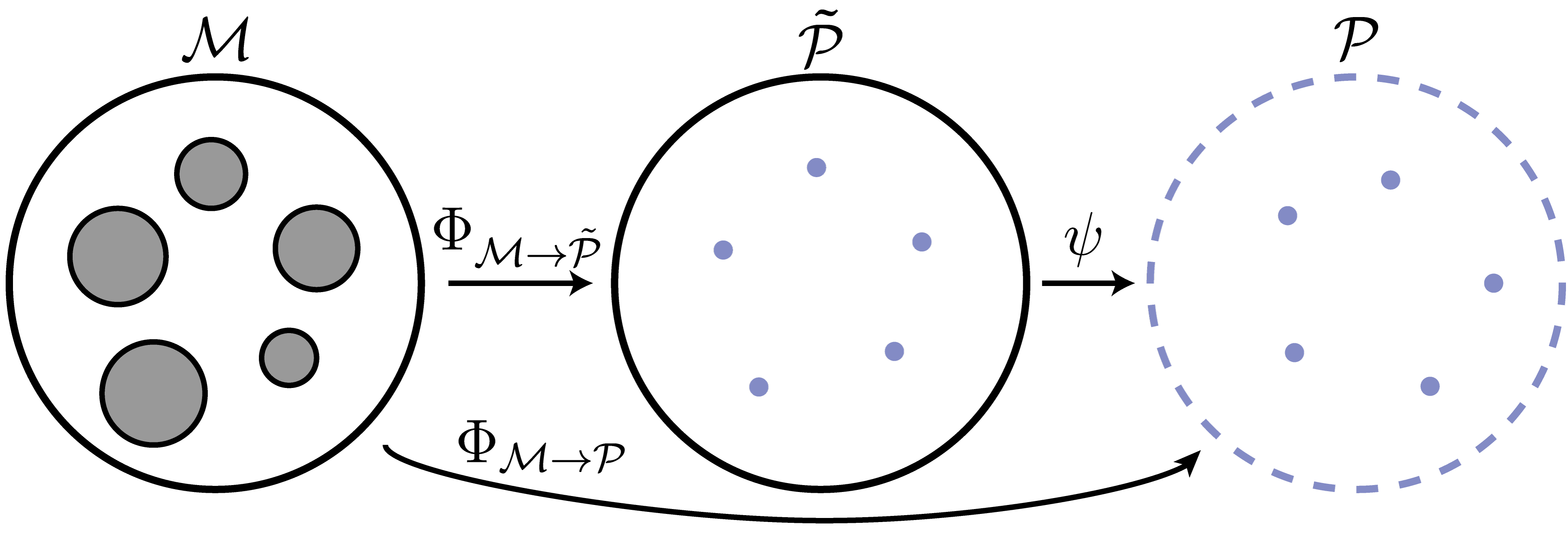
Figure 2: Illustration of diffeomorphic transformation from sphere word $\mathcal{M}$ to unbounded point world $\tilde{\mathcal{P}}$ and to unbounded point world $\mathcal{P}$.

Definition 1.

The harmonic potential function in a point world, denoted by $\phi_{\mathcal{P}}:\mathcal{P}\rightarrow\mathbb{R}^{+}$, is defined as:

$$\phi_{\mathcal{P}}(x)\triangleq\phi(x,\,P_{G})-\frac{1}{K}\sum_{i=1}^{M}\phi(x,P_{i}),$$ (2)

where $\phi(x,\,q)=\ln\left(\|x-q\|^{2}\right)$ is the primitive harmonic function for $x,\,q\in\mathbb{R}^{2}$; $\phi(x,\,P_{G})$ is the potential for the transformed goal $P_{G}=\Phi_{\mathcal{M}\rightarrow\mathcal{P}}(q_{G})$, whereas $\phi(x,\,P_{i})$ for the obstacle $P_{i}$, where $i=1,\cdots,M$; $K\geq 1$ is a tuning parameter. $\blacksquare$

Lastly, the logistic function is used to transform the unbounded range of $\phi_{\mathcal{P}}$ to a finite interval $[0,\,\mu]$ for $\mu\geq 1$.

2.2 Linear Temporal Logic and Büchi Automaton

The basic ingredients of Linear Temporal Logic (LTL) formulas are a set of atomic propositions $AP$, and several Boolean or temporal operators. Atomic propositions are Boolean variables that can be either true or false. The syntax of LTL is defined as: $\varphi\triangleq\top\;|\;p\;|\;\varphi_{1}\wedge\varphi_{2}\;|\;\neg\varphi\;|\;\bigcirc\varphi\;|\;\varphi_{1}\,\textsf{U}\,\varphi_{2}$, where $\top\triangleq\texttt{True}$, $p\in AP$, $\bigcirc$ (next), U (until) and $\bot\triangleq\neg\top$. The derivations of other operators, such as $\Box$ (always), $\Diamond$ (eventually), $\Rightarrow$ (implication) are omitted here for brevity. A complete description of the semantics and syntax of LTL can be found in Baier & Katoen (2008). Moreover, there exists a Nondeterministic Büchi Automaton (NBA) for formula $\varphi$ as follows:

Definition 2.

A NBA $\mathcal{A}\triangleq(S,\,\Sigma,\,\delta,\,(S_{0},\,S_{F}))$ is a 4-tuple, where $S$ are the states; $\Sigma=AP$; $\delta:S\times\Sigma\rightarrow 2^{S}$ are transition relations; $S_{0},S_{F}\subseteq S$ are initial and accepting states. $\blacksquare$

An infinite word $w$ over the alphabet $2^{AP}$ is defined as an infinite sequence $W=\sigma_{1}\sigma_{2}\cdots,\sigma_{i}\in 2^{AP}$. The language of $\varphi$ is defined as the set of words that satisfy $\varphi$, namely, $\mathcal{L}=Words(\varphi)=\{W\,|\,W\models\varphi\}$ and $\models$ is the satisfaction relation. Additionally, the resulting run of $w$ within $\mathcal{A}$ is an infinite sequence $\rho=s_{0}s_{1}s_{2}\cdots$ such that $s_{0}\in S_{0}$, and $s_{i}\in S$, $s_{i+1}\in\delta(s_{i},\,\sigma_{i})$ hold for all index $i\geq 0$. A run is called accepting if it holds that $\inf(\rho)\cap{S}_{F}\neq\emptyset$, where $\inf(\rho)$ is the set of states that appear in $\rho$ infinitely often. In general, an accepting run has the prefix-suffix structure from an initial state to an accepting state that is contained in a cyclic path. Typically, the size of $\mathcal{A}$ is double exponential to the length of formula $\varphi$.

3 Problem Description

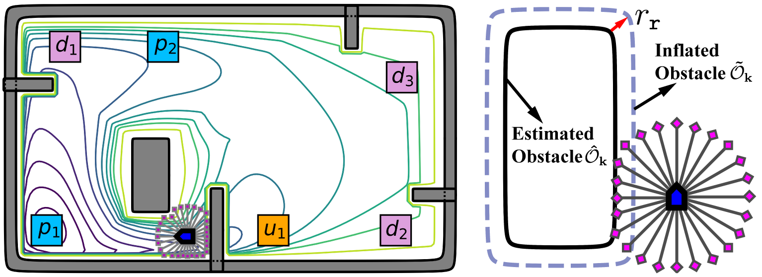
Figure 3: Left: Robot in the initially-known workspace with overlapping obstacles and several regions of interest. Right: Reconstruction of obstacle model.

Consider a mobile robot that occupies a circular area with radius $r_{\texttt{r}}>0$ and follows the unicycle dynamics:

$$\dot{x}=\upsilon\cos(\theta),\;\dot{y}=\upsilon\sin(\theta),\;\dot{\theta}=\omega,$$ (3)

where $q=(x,\,y)\in\mathcal{W}$ is the robot position and $\theta\in[-\pi,\pi]$ as its orientation; $(\upsilon,\,\omega)$ are its linear and angular velocities as control inputs. The workspace $\mathcal{W}_{0}\subset\mathbb{R}^{2}$ is compact and connected, with $M$ internal obstacles $\mathcal{O}_{i}$ such that $\mathcal{O}_{i}\subset\mathcal{W}_{0}$ and $\mathcal{O}_{i}\bigcap\mathcal{O}_{j}=\emptyset$, $i\neq j$, $\forall i,j\in\{1,\cdots,M\}$. Considering the robot size, the outer workspace $\mathcal{W}_{0}$ and inner obstacle $\mathcal{O}_{i}$ are inflated by a margin $r_{\texttt{r}}$, denoted by $\tilde{\mathcal{W}}_{0}$ and $\tilde{\mathcal{O}}_{i}$. Therefore, the feasible workspace is given by $\mathcal{W}\triangleq\tilde{\mathcal{W}}_{0}\backslash\bigcup_{i=1}^{M}\tilde{\mathcal{O}}_{i}$.

Initially at $t=0$, the workspace is only partially known to the robot, i.e., the outer boundary and some inner obstacles. Starting from any valid initial state $(q_{0},\,\theta_{0})$, the robot can navigate within the workspace and observe more obstacles, via a range-limited sensor modeled as follows:

$$\mathcal{S}(q)\triangleq\left\{\hat{q}\in\mathcal{W}\,|\,\left(\hat{q}\in\mathcal{D}_{r_{\texttt{s}}}(q)\right)\wedge\left(\mathcal{L}(q,\,\hat{q})\subset\mathcal{W}\right)\right\},$$ (4)

where $\mathcal{S}(q)$ is the set of boundary points $\hat{q}$ observed by the robot at position $q\in\mathcal{W}$; $\mathcal{D}_{r_{\texttt{s}}}(q)$ is a disk centered at $q$ with radius $r_{\texttt{s}}$ and $\mathcal{L}(q,\,\hat{q})$ is the straight line connecting $q$ and $\hat{q}$. As shown in Fig. 3, it returns the 2D point cloud from the robot to any blocking surface within the sensing range. This model mimics a $360^{\circ}$ Lidar scanner as also used in Rousseas et al. (2022b).

Lastly, there is a set of non-overlapping regions of interest $g_{n}\subset\mathcal{W}$, $n=1,\cdots,N$. With slight abuse of notation, the associated atomic propositions are also denoted by $G=\{g_{n}\}$, standing for “the robot is within region $g_{n}$, i.e., $q\in g_{n}$”. The desired task is specified as a LTL formula $\varphi$ over $G$, i.e., $\varphi=LTL(G)$ by the syntax described in Sec. 2.2. Given the robot trajectory $\mathbf{q}$, its trace is given by the sequence of regions over time, i.e., $\omega(\mathbf{q})=g_{\ell_{1}}g_{\ell_{2}}\cdots$, where $g_{\ell_{k}}\in G$ and $q(t_{k})\in g_{\ell_{k}}$, for some time instants $0\leq t_{k}\leq t_{k+1}$ and $k\in\mathbb{Z}$.

Thus, the objective is to design an online control and planning strategy for system (3) such that starting from an initial pose $(q_{0},\,\theta_{0})$, the trace of the resulting trajectory $\omega(\mathbf{q})$ fulfills the given task $\varphi$, while avoiding collision with all obstacles.

4 Proposed Solution

As illustrated in Fig. 1, the proposed solution is a hybrid control framework as two-layer harmonic trees (HT) that combines harmonic potentials for navigation and oriented search trees for planning. Initially, the automaton-guided search trees and the orientation-aware harmonic potentials are constructed in a dependent manner given the partially-known workspace. Then, as the robot explores more obstacles, an online adaptation scheme is proposed to revise the search tree and update the harmonic potentials recrusively and simultaneously.

4.1 Initial Synthesis

This section presents the algorithmic details of the initial planning and control strategy. First, the automaton-guided harmonic trees are constructed given the task automaton and the set of intermediate waypoints, within which the initial discrete plan is derived. Then, a novel method to construct orientation-aware harmonic potentials is introduced, based on which a nonlinear controller is designed for full-state navigation.

4.1.1 Two-layer and Automaton-guided Harmonic Trees

As described in Sec. 2.2, the NBA associated with $\varphi$ is given by $\mathcal{A}_{\varphi}=(S,\,\Sigma,\,\delta,\,(S_{0},\,S_{F}))$, which captures all potential traces that satisfy the task. To begin with, the initial navigation map is constructed as a weighted and fully-connected graph $\mathcal{G}\triangleq(\widehat{G},\,E,\,d,\,(g_{0},\theta_{0}))$, where: (i) $\widehat{G}=G\times\Theta$ is the set of regions of interest plus a set of orientations $\Theta\subset[0,2\pi)$; (ii) $E\subset\widehat{G}\times\widehat{G}$ is the set of transitions; (iii) $d:E\rightarrow\mathbb{R}^{+}$ is the cost function, which is initialized as $d((g,\theta),\,(g^{\prime},\theta^{\prime}))\triangleq\|g-g^{\prime}\|_{2}+w|\theta-\theta^{\prime}|$, $\forall(g,\theta),\,(g^{\prime},\theta^{\prime})\in\widehat{G}$ and parameter $w>0$; and $(g_{0},\theta_{0})$ is the initial pose. Note that $E$ is initialized as fully-connected since the actual feasibility can only be determined after the associated controllers are constructed. Due to the same reason, the navigation cost is estimated by the Euclidean distance initially, and later updated online.

Given $\mathcal{G}$ and $\mathcal{A}_{\varphi}$, the standard model-checking procedure is followed to find the task plan. Namely, their synchronized product is built as $\widehat{\mathcal{A}}\triangleq\mathcal{G}\times\mathcal{A}_{\varphi}=(\widehat{S},\,\widehat{\delta},\,\widehat{d},\,(\widehat{S}_{0},\widehat{S}_{F}))$, where $\widehat{S}=\widehat{G}\times S$; $\widehat{S}_{0},\widehat{S}_{F}\subset\widehat{S}$ are the sets of initial and accepting states; $\widehat{\delta}\subset\widehat{S}\times\widehat{S}$ that $(\langle g,s\rangle,\langle g^{\prime},s^{\prime}\rangle)\in\widehat{\delta}$ if $(g,g^{\prime})\in E$ and $s^{\prime}\in\delta(s,\{g\})$; $\widehat{d}(\langle g,s\rangle,\langle g^{\prime},s^{\prime}\rangle)=d(g,g^{\prime})$, $\forall(\langle g,s\rangle,\langle g^{\prime},s^{\prime}\rangle)\in\widehat{\delta}$. Note that the product $\mathcal{\widehat{A}}$ is still a Büchi automaton, of which the accepting run satisfies the prefix-suffix structure. Namely, consider the following run of $\widehat{\mathcal{A}}$: $\widehat{\mathbf{S}}=\widehat{s}_{1}\widehat{s}_{2}\cdots\widehat{s}_{L}(\widehat{s}_{L+1}\widehat{s}_{L+2}\cdots$ $\widehat{s}_{L+H})^{\omega}$, which an infinite sequence of $\widehat{S}$ with $\widehat{s}_{1}\cdots\widehat{s}_{L}$ being the prefix and $\widehat{s}_{L+1}\cdots\widehat{s}_{L+H}$ being the suffix repeated infinitely often; $\widehat{s}_{1}\in\widehat{S}_{0}$ and $\widehat{s}_{L+1}\in\widehat{S}_{F}$; and $L,H\geq 1$. A nested Dijkstra algorithm is used to find the best pair of initial and accepting states $(\widehat{s}^{\star}_{0},\widehat{s}^{\star}_{F})$. Thus, the optimal plan given the initial environment is obtained by projecting $\widehat{\mathbf{S}}$ onto $\widehat{G}$, i.e.,

$$\widehat{\mathbf{g}}=\widehat{g}_{1}\widehat{g}_{2}\cdots\widehat{g}_{L}(\widehat{g}_{L+1}\widehat{g}_{L+2}\cdots\widehat{g}_{L+H})^{\omega},$$ (5)

where $\widehat{g}_{\ell}=\widehat{s}_{\ell}|_{\widehat{G}}$ are the regions. More algorithmic details can be found in Guo & Dimarogonas (2015).

The obtained plan $\widehat{\mathbf{g}}$ can be executed by sequentially traversing the transitions $(\widehat{g}_{\ell},\,\widehat{g}_{\ell+1})$, by designing appropriate potential fields as in Loizou & Rimon (2022); Rousseas et al. (2021) However, as mentioned in Sec. 1.1, when $\widehat{g}_{\ell},\,\widehat{g}_{\ell+1}$ are far away within a partially-known workspace, the resulting trajectory may suffer from oscillation or jitters and long detours. To tackle these issues, the structure of oriented harmonic trees (HT) is proposed. More specifically, the oriented HT associated with $(\widehat{g}_{\ell},\,\widehat{g}_{\ell+1})$ is a tree structure defined by a 4-tuple:

$$\mathcal{T}_{\widehat{g}_{\ell}\rightarrow\widehat{g}_{\ell+1}}\triangleq\big{(}V,\,B,\,\gamma,\,(\nu_{0},\,\nu_{G})\big{)},$$ (6)

where $V\subset\mathcal{W}\times(-\pi,\,\pi]$ is the set of vertices; $B\subset V\times V$ is the set of edges; $\gamma:B\rightarrow\mathbb{R}_{\geq 0}$ returns the edge cost to be estimated; $\nu_{0}=\widehat{g}_{\ell}$ and $\nu_{G}=\widehat{g}_{\ell+1}$ are the initial and target poses. The goal is to find a sequence of vertices in $\mathcal{T}$ as the path from $\nu_{0}$ to $\nu_{G}$. Initially, $V=\{\nu_{0},\,\nu_{G}\}$ and $B=\emptyset$. Then, the set of vertices can be generated in various ways, e.g., via direct discretization including uniform, triangulation and voronoi partitions, see e.g., LaValle (2006); or sampling-based methods such as PRM from Hsu et al. (2006) and RRT from Karaman & Frazzoli (2011). In other words, the oriented HT is not limited to one particular choice of abstraction method. It is worth mentioning that these vertices should be augmented by orientations if not already. Afterwards, any vertex is connected to all vertices within its free vicinity, i.e., $(\nu,\,\nu^{\prime})\in B$ if $\|\nu-\nu^{\prime}\|<\varepsilon$ holds for a radius $\varepsilon>0$. For each edge $(\nu,\,\nu^{\prime})\in E$, the control cost $\gamma(\nu,\,\nu^{\prime})$ for the robot (3) to navigate from $\nu$ to $\nu^{\prime}$ is derived in the sequel. Thus, given the weighted and directed tree $\mathcal{T}_{\widehat{g}_{\ell}\rightarrow\widehat{g}_{\ell+1}}$, the shortest path from $\nu_{0}$ to $\nu_{G}$ can be determined by any search algorithm from LaValle (2006), e.g., Dijkstra and A^⋆ (with $\|\nu-\nu_{G}\|$ being the “cost-to-go” heuristic). The resulting path is denoted by:

$$\mathbf{P}_{\widehat{g}_{\ell}\rightarrow\widehat{g}_{\ell+1}}\triangleq\nu_{0}\nu_{1}\cdots\nu_{N-1}\nu_{G},$$ (7)

where $\nu_{n}\in V$ and $(\nu_{n},\,\nu_{n+1})\in B$, $\forall n\in[0,\,N-1]$. In other words, each vertex along the path serves as the intermediate waypoints to navigate from region $\widehat{g}_{\ell}$ to $\widehat{g}_{\ell+1}$.

4.1.2 Orientation-aware Harmonic Potentials

As explained in (4), a 2D point cloud is returned that consists of points on any obstacle surface within the sensing range. More specifically, denoted by $\mathbf{D}_{t}=\{d_{j}\}$ the set of 2D points that are already transformed from the local coordinate to global coordinate where $d_{j}\in\partial\mathcal{W}$. To begin with, these data points are divided into $K$ clusters representing $K$ separate obstacles, i.e., $\mathbf{D}_{t}=\{\mathbf{D}_{t,k}\}$, by e.g., checking the relative distance and change of slope between consecutive points. The exact thresholds would depend on the specification of the Lidar scanner. Then, each cluster is fitted to a particular 2D obstacle. This work primarily focuses on a special type of obstacle called squircle. Squircles are particularly useful for representing walls and corners, see Li & Tanner (2018). As shown in Fig. 4, a squircle interpolates smoothly between a circle and a square, while avoiding non-differentiable corners. In particular, a unit squircle centered at the origin in $\mathbb{R}^{2}$ is given by:

$$\beta_{\texttt{sc}}(q)\triangleq\frac{q^{2}+\sqrt{q^{4}-4\varkappa^{2}\,{[(q^{\intercal}\,e_{1})(q^{\intercal}\,e_{2})]}^{2}}}{2}-1,$$ (8)

where $\varkappa\in(0,\,1)$ is a positive parameter; $e_{1}\triangleq[1,0]^{\intercal}$ and $e_{2}\triangleq[0,1]^{\intercal}$ are two unit basis in $\mathbb{R}^{2}$. Non-unit squircles with general centers can be derived via scaling $\mathbf{A}$ and translation $\mathbf{T}$, i.e., $\mathbf{A}\triangleq\text{diag}(\mathbf{s})$ and $\mathbf{T}\triangleq\mathbf{c}^{\intercal}$, where $\mathbf{s}\triangleq(a^{1},\,a^{2})$ represents the width and height of the squircle; $\mathbf{c}\triangleq(c^{1},\,c^{2})$ is the geometric center of the squircle. Given the clusters of the observed point clouds, the model of obstacles can be reconstructed based on the above model of squircle, as illustrated in Fig. 3.

Lemma 1.

Given a cluster of point cloud $\mathbf{D}_{t,k}=\{q_{1},q_{2},\cdots,$ $q_{N}\}$ associated with the same squircle obstacle, if $N\geq 4$ and $q_{i}\neq q_{j}$, $i\neq j$, $\forall i,j\in\{1,\cdots,N\}$, then this obstacle can be uniquely reconstructed as $\hat{\mathcal{O}}_{k}\triangleq(\mathbf{s}_{k},\,\mathbf{c}_{k})$, i.e., the scaling $\mathbf{A}_{k}$ and translation $\mathbf{T}_{k}$ can be uniquely determined.

Proof.

Since the cluster of points lay on the surface of the squircle obstacle, each point $q_{i}\in\mathbf{D}_{t,k}$ satisfies: $\beta_{\texttt{sc}}(\hat{q}_{i})=0$ holds for $\hat{q}_{i}=\mathbf{A}^{-1}_{k}(q_{i}-\mathbf{c}_{k})$. It can be further derived as: $[a_{k}^{2}(x_{i}-c_{k}^{1})]^{2}+[a_{k}^{1}(y_{i}-c_{k}^{2})]^{2}-(a_{k}^{1}\,a_{k}^{2})^{2}-\varkappa^{2}[(x_{i}-c_{k}^{1})(y_{i}-c_{k}^{2})]^{2}=0$, $\forall i=1,\cdots,N$. The above $N$ equations include four solving variables $a_{k}^{1},a_{k}^{2},c_{k}^{1},c_{k}^{2}$. By the Gröbner bases, any four of these equations yield a unique solution, denoted by $(\hat{a}_{k}^{1},\hat{a}_{k}^{2},\hat{c}_{k}^{1},$ $\,\hat{c}_{k}^{2})=(\mathbf{\hat{s}}_{k},\,\mathbf{\hat{c}}_{k})$. Then, the obstacle is reconstructed by (8). ∎

Remark 1.

In practice, the point-cloud data might be noisy and not align with a squircle perfectly. Higher accuracy can be achieved by using more data points by the optimization method like Levenberg-Marquardt algorithm from Gavin (2019). $\blacksquare$

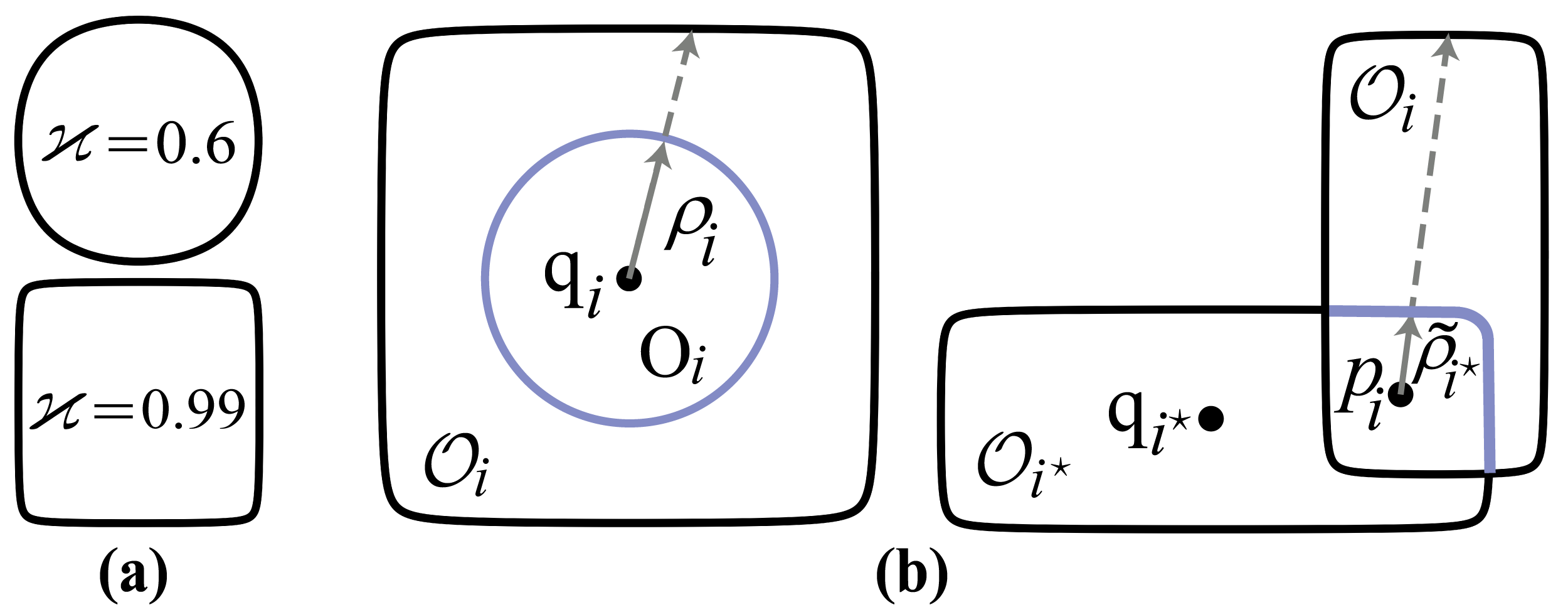
Figure 4: (a) Squircles with the parameter $\varkappa=0.6$ and $\varkappa=0.99$; (b) Ray scaling process. The boundary of the star-shaped obstacle is mapped onto the boundary of a sphere (Left). The boundary of the child obstacle is mapped onto a segment of the boundary of the parent obstacle (Right).

Consequently, denote by $\{\hat{\mathcal{O}}_{t}\}$ the collection of obstacles detected and fitted at time $t\geq 0$. An example is shown in Fig. 3, where an initial workspace model is constructed given the sensory data at $t=0$. Given the set of squircle obstacles $\{\hat{\mathcal{O}}_{0}\}$, the initial navigation function $\varphi_{\texttt{NF}}(q)$ is constructed by three major diffeomorphic transformations: (i) $\Phi_{\mathcal{F}\rightarrow\mathcal{S}}$ transforms the forest of stars into a star world via “purging”; (ii) $\Phi_{\mathcal{S}\rightarrow\mathcal{M}}$ transforms the star world into its model sphere world; and (iii) $\Phi_{\mathcal{M}\rightarrow\mathcal{P}}$ transforms the sphere world into a point world. The complete navigation function for the original workspace is given by:

$$\varphi_{\texttt{NF}}(q)=\sigma\circ\phi_{\mathcal{P}}\circ\Phi_{\mathcal{M}\rightarrow\mathcal{P}}\circ\Phi_{\mathcal{S}\rightarrow\mathcal{M}}\circ\Phi_{\mathcal{F}\rightarrow\mathcal{S}}(q),$$ (9)

where $\sigma\circ\phi_{\mathcal{P}}$ is defined in (2); and the transformation $\Phi_{\mathcal{M}\rightarrow\mathcal{P}}$ is given in (1). The remaining part of this section describes the two essential and nontrivial transformations $\Phi_{\mathcal{S}\rightarrow\mathcal{M}}$ and $\Phi_{\mathcal{F}\rightarrow\mathcal{S}}$.

Star-to-Sphere Transformation. The star world $\mathcal{S}$ has an outer boundary of squircle workspace $\mathcal{O}_{0}=\{q\in\mathbb{R}^{2}|\beta_{0}(q)\leq 0\}$ and $M$ inner squircle obstacles $\mathcal{O}_{i}=\{q\in\mathbb{R}^{2}|\beta_{i}(q)\leq 0\}$, where $\beta_{i}(q)$ is the obstacle function defined in (8), for $i=0,1,\cdots,M$. The star-to-sphere transformation is constructed by the ray scaling process from Rimon (1990), as shown in Fig. 4. To begin with, define the following scaling factor:

$$v_{0}(q)\triangleq\rho_{0}\frac{1-\beta_{0}(q)}{||q-\mathbf{c}_{0}||},\quad v_{i}(q)\triangleq\rho_{i}\frac{1+\beta_{i}(q)}{||q-\mathbf{c}_{i}||},$$ (10)

where $\mathbf{c}_{i}$ is the geometric center of the associated squircle and $\rho_{i}$ is the radius of the transformed sphere. Moreover, the translated scaling map $T_{i}$ for each obstacle $\mathcal{O}_{i}$ is defined by:

$$T_{i}(q)\triangleq v_{i}(q)\,(q-\mathbf{c}_{i})+\mathbf{c}_{i},$$ (11)

for $i=0,1,\cdots,M$. Consequently, the transformation from star world $\mathcal{S}$ to its model sphere world $\mathcal{M}$ is given by:

$$\Phi_{\mathcal{S}\rightarrow\mathcal{M}}\triangleq\Big{(}1-\sum_{i=0}^{M}\sigma_{i}(q)\Big{)}\,{\rm id}(q)+\sum_{i=0}^{M}\sigma_{i}(q)\,T_{i}(q),$$ (12)

where $\sigma_{i}(q)\triangleq\frac{\gamma_{G}(q)\overline{\beta}_{i}(q)}{\gamma_{G}(q)\overline{\beta}_{i}(q)+\lambda\beta_{i}(q)}$ is the analytic switch for the workspace boundary and obstacles; ${\rm id}(q)$ is the identity function; $\lambda>0$ is a parameter; $\gamma_{G}(q)\triangleq\|q-q_{G}\|^{2}$ is the distance-to-goal; and $\overline{\beta}_{i}(q)\triangleq\prod_{j=0,j\neq i}^{M}\beta_{j}(q)$ is the omitted product.

Leaf-Purging Transformation. As described in Loizou & Rimon (2022); Li & Tanner (2018); Rimon (1990), besides disjointed star worlds, it is essential to consider the workspace formed by unions of overlapping stars, called the forest of stars. It consists of several disjointed clusters of obstacles as trees of stars, which in turn is a finite union of overlapping star obstacles whose adjacency graph is a tree. Since overlapping stars can not be transformed directly as a whole obstacle, each tree has to be transformed via successively purging its leaves. Specifically, a forest of stars is described by $\mathcal{F}=\mathcal{W}_{0}\backslash\bigcup_{n=1}^{N}\mathcal{T}_{n}$, where $\mathcal{T}_{n}$ is the $n$-th tree of stars among the $N$ trees. Each tree of stars has a unique root, and its obstacles are arranged in a parent-child relationship. An example is shown in Fig. 5, where the trees have different depths according to the level of leaves in the tree. Without loss of generality, denote by $d_{n}$ the depth of the tree $\mathcal{T}_{n}$ and $\mathcal{L}$ the set of indices for all leaf obstacles in all trees, and by $\mathcal{I}$ the set of indices associated with all obstacles within $\mathcal{F}$. Furthermore, denote by $\mathcal{O}_{i}\triangleq\{q\in\mathbb{R}^{2}:\beta_{i}(q)\leq 0\}$ the leaf obstacles, where $\beta_{i}(q)$ is the obstacle function defined in (8). The parent of obstacle $\mathcal{O}_{i}$ is denoted by $\mathcal{O}_{i^{\star}}$, of which the centers are chosen to be the same and denoted by $p_{i}\in\mathcal{O}_{i}\bigcap\mathcal{O}_{i^{\star}}$. Then, the diffeomorphic transformation from the forest of stars $\mathcal{F}$ to the star world $S$ is constructed via the successive purging transformations for each tree as follows:

$$\Phi_{\mathcal{F}\rightarrow\mathcal{S}}(q)\triangleq\Phi_{N}\circ\cdots\Phi_{2}\circ\Phi_{1}(q),$$ (13)

where $\Phi_{n}(q)$ is the purging transformation for the $n$-th tree of stars, where $n=1,\cdots,N$. It has the following format:

$$\Phi_{n}(q)\triangleq f_{n,1}\circ f_{n,2}\cdots\circ f_{n,d_{n}}(q),$$ (14)

where $f_{n,i}(q)$ is the purging transformation for the $i$-th leaf obstacle in the $n$-th tree for $i=1,\cdots,d_{n}$, which is constructed by the ray-scaling process to purge the leaf obstacle into its parent as shown in Fig 4. Due to the specific representation of the squircle, the length of rays from the common center $p_{i}$ to the boundary of the parent obstacle $\mathcal{O}_{i^{\star}}$, is calculated by:

$$\tilde{\rho}_{i^{\star}}(\hat{q})\triangleq\frac{1}{\|\tilde{\mathbf{A}}_{i^{\star}}^{-1}\hat{q}\|}\,\rho_{sc}\left(\frac{\tilde{\mathbf{A}}_{i^{\star}}^{-1}\hat{q}}{\|\tilde{\mathbf{A}}_{i^{\star}}^{-1}\hat{q}\|}\right),$$ (15)

where $\hat{q}=\frac{q-p_{i}}{\|q-p_{i}\|}$ is the normalized vector of $q-p_{i}$; $\rho_{sc}(\cdot)$ is the length of the rays for unit squircle drived from (8); and $\tilde{\mathbf{A}}_{i^{\star}}\in\mathbb{R}^{2\times 2}$ is a piecewise scaling matrix tailored for the parent squircle which is diagonal with the following entries:

$$\tilde{a}_{i^{\star}}^{\ell}(\hat{q})\triangleq a_{i^{\star}}^{\ell}+\mathbf{sgn}(\hat{q}^{\intercal}e_{\ell})[\mathbf{c}_{i^{\star}}-p_{i}]^{\intercal}e_{\ell},$$ (16)

for $\ell=1,2$, where $a_{i^{\star}}^{\ell}$ are the entries of the diagonal scaling matrix $\mathbf{A}_{i^{\star}}$ of the parent squircle; $\mathbf{c}_{i^{\star}}$ is the geometric center of the parent obstacle; and $e_{\ell}$ are two base vectors for $\ell=1,2$.

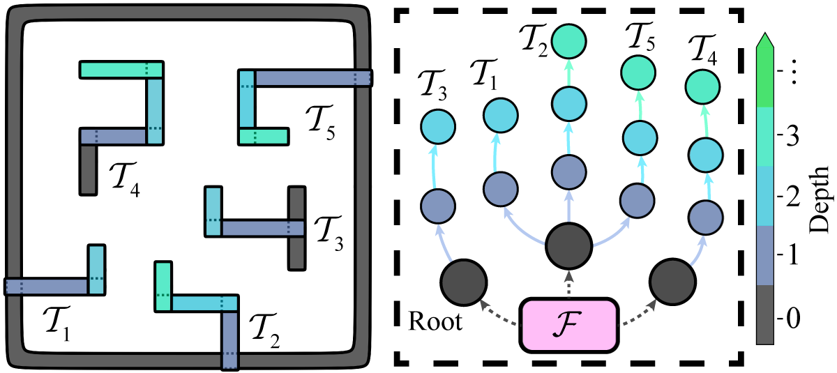
Figure 5: A forest world $\mathcal{F}$ with overlapping squircles (Left), which consists of $5$ trees of stars $\mathcal{T}_{i}$ with different depths from the root to the leaves (Right).

Lemma 2.

The length of rays $\tilde{\rho}_{i^{\star}}(q)$ is smooth in $\mathcal{W}_{0}\backslash\mathcal{O}_{i}\bigcup\mathcal{O}_{i^{\star}}$.

Proof.

The derivative of $\tilde{\rho}_{i^{\star}}(q)$ is given by the chain rule:

$$\nabla\tilde{\rho}_{i^{\star}}(q)=\frac{\|q-p_{i}\|^{2}\mathbf{I}-(q-p_{i})(q-p_{i})^{\intercal}}{\|q-p_{i}\|^{3}}\nabla\tilde{\rho}_{i^{\star}}(\hat{q}),$$

where the derivative of $\tilde{\rho}_{i^{\star}}(\hat{q})$ boils down to computing the derivatives of $\rho_{sc}(q)$ and $Z(\hat{q})=\tilde{\mathbf{A}}_{i^{\star}}^{-1}\hat{q}$ in (15). The smoothness of $\rho_{sc}(q)$ and its derivative can be obtained directly from (8). Since $\nabla a_{i^{\star}}^{\ell}(\hat{q})=\nabla(a_{i^{\star}}^{\ell}+\mathbf{sign}(\hat{q}^{\intercal}e_{\ell})[q_{i^{\star}}-p_{i}]^{\intercal}e_{\ell})=0$, for $\ell=1,2$, the derivative of $Z(\hat{q})$ is calculated and simplified as:

$$\nabla Z(\hat{q})=\tilde{\mathbf{A}}_{i^{\star}}^{-1}\mathbf{I}-\tilde{\mathbf{A}}_{i^{\star}}^{-1}[\nabla\tilde{\mathbf{A}}_{i^{\star}}]\tilde{\mathbf{A}}_{i^{\star}}^{-1}\hat{q}=\tilde{\mathbf{A}}_{i^{\star}}^{-1}.$$

Besides, as $\|q-p_{i}\|>0$ holds for every point $q\in\mathcal{W}_{0}\backslash\mathcal{O}_{i}\bigcup\mathcal{O}_{i^{\star}}$, the derivative of $\tilde{\rho}_{i^{\star}}(q)$ exists and is well-defined. On the other hand, $\nabla\tilde{\rho}_{i^{\star}}(q)$ is continuous since its compositions are all continuous. Therefore, $\tilde{\rho}_{i^{\star}}(q)$ is at least $C^{1}$ smooth. Additionally, higher-order smoothness can be proven by the same procedure, which is omitted here. ∎

Remark 2.

The modified length of rays $\tilde{\rho}_{i^{\star}}(q)$ in (15) is essential since the common center $p_{i}$ is not always aligned with the geometric center $q_{i^{\star}}$ of the parent obstacle. A similar technique is introduced in Li & Tanner (2018) via a virtual obstacle between the parent and son obstacles. In contrast, the piecewise scaling matrix proposed here in (15) is less conservative and computationally more efficient. $\blacksquare$

Given the length of rays $\tilde{\rho}_{i^{\star}}(q)$, the star deforming factor for each leaf obstacle $\mathcal{O}_{i}$ is calculated by:

$$v_{i}(q)=\tilde{\rho}_{i^{\star}}(q)\,\frac{1+\beta_{i}(q)\tilde{\kappa}_{i}(q)}{\|q-p_{i}\|},$$ (17)

where $\tilde{\kappa}_{i}(q)$ is defined by: $\tilde{\kappa}_{i}(q)\triangleq\beta_{i^{\star}}(q)+(\beta_{i}(q)-2E_{i})+\sqrt{\beta^{2}_{i^{\star}}(q)+((\beta_{i}(q)-2E_{i}))^{2}}.$ The parameter $E_{i}>0$ is a geometric constant satisfying that $\mathcal{O}_{i}(2E_{i})\bigcap\mathcal{O}_{j}(2E_{j})=\emptyset$ and $\gamma^{-1}([0,2E_{d}])\bigcap\mathcal{O}_{i}(2E_{i})=\emptyset$ with $E_{d}>0$ being a geometric constant and $\mathcal{O}_{i}(2E_{i})\triangleq\{q\in\mathbb{R}^{2}|\beta_{i}(q)\leq 2E_{i}\}$ for $i,\,j\in\mathcal{I}$ with $i\neq j\,$ and $i,j\neq j^{\star}$. Furthermore, the translated scaling map $T_{i}$ for each obstacle $\mathcal{O}_{i}$ with the common center $p_{i}$ is defined by:

$$T_{i}(q)\triangleq v_{i}(q)\,(q-p_{i})+p_{i}.$$ (18)

Therefore, the purging transformation $f_{n,i}(q)$ for the $i$-th leaf obstacle $\mathcal{O}_{i}$ in the $n$-th tree is defined by:

$$f_{n,i}(q)\triangleq\big{(}1-\sigma_{i}(q,\xi_{i})\big{)}\,{\rm id}(q)+\sigma_{i}(q,\xi_{i})\,T_{i}(q),$$ (19)

where $\sigma_{i}(q,\xi_{i})\triangleq\frac{\gamma_{G}(q)\overline{\beta}_{i}(q)}{\gamma_{G}(q)\overline{\beta}_{i}(q)+\xi_{i}\beta_{i}(q)}$ is the analytic switch; $\xi_{i}>0$ is a positive parameter; $\gamma_{G}(q)$ is the same as in (12); and $\overline{\beta}_{i}(q)$ is the omitted product defined by:

$$\overline{\beta}_{i}(q)\triangleq\Big{(}\prod_{j\in\mathcal{I}\backslash\{i,i^{\star}\}}\beta_{j}(q)\Big{)}\Big{(}\prod_{j\in\mathcal{L}\backslash\{i\}}\beta_{j}(q)\Big{)}\tilde{\beta}_{i}(q),$$

where $\tilde{\beta}_{i}(q)$ with a geometric constant $E_{i}>0$ is defined by: $\tilde{\beta}_{i}(q)\triangleq\beta_{i^{\star}}(q)+(2E_{i}-\beta_{i}(q))+\sqrt{\beta^{2}_{i^{\star}}(q)+(2E_{i}-\beta_{i}(q))^{2}}.$

Remark 3.

The original purging method proposed in Rimon (1990) deals with overlapping obstacles via Boolean combinations and applies only to planar and parabolic obstacles. The work in Li & Tanner (2018) proposes a simpler method for computing the ray scaling transformations using varying ray lengths. However, these approaches purge all the leaves at once, which is not applicable to the dynamic scenarios where the obstacles are added to the workspace one by one. Thus, a novel method is proposed in (19) that purges the leafs one by one. $\blacksquare$

Remark 4.

Recently, a novel conformal transformation was introduced in Fan et al. (2022) to map the complex workspace to a sphere world without the decomposition of tree of stars. However, this approach requires a numerical solution of continuous integral equations, which is time-consuming and not applicable to unknown environment. Conversely, the proposed method offers an analytical solution, making it superior for navigation in unknown scenarios. $\blacksquare$

Lemma 3.

Given a workspace $\mathcal{W}$ containing $N$ tree-of-stars with different depth $d_{n}\geq 0$, for $n=1,\cdots N$, the complete harmonic potential function $\varphi_{\texttt{NF}}(q)$ in (9) is a valid navigation function for the workspace $\mathcal{W}$, if the parameters $K>N$ and $\mu\geq 1$ hold in (2); $\lambda>\Lambda$ for a positive number $\Lambda>0$; and $\xi_{i}>\Xi_{i}$ for some positive numbers $\Xi_{i}>0$, for $i=0,\cdots,d_{n}$.

Proof.

Similar statements have been proven in Rousseas et al. (2021); Filippidis & Kyriakopoulos (2011); Loizou & Rimon (2022), thus detailed proofs are omitted here and refer the readers to e.g., Theorem 1 of Loizou & Rimon (2022), Theorem 2 in Li & Tanner (2018) and Proposition 5 of Loizou (2017). Briefly speaking, it is shown that the transformation $\Phi_{\mathcal{S}\rightarrow\mathcal{M}}$ $\Phi_{\mathcal{F}\rightarrow\mathcal{S}}$ are diffeomorphic as long as $\lambda>\Lambda$ and $\xi_{i}>\Xi_{i}$ for some sufficient large numbers $\Lambda$ and $\Xi_{i}$, and the final potential function $\varphi_{\texttt{NF}}(q)$ has a unique global minimum at the goal $q_{\texttt{G}}$ and more importantly, a set of isolated saddle points of measure zero if $K>N$ and $\mu\geq 1$ hold. Since the purging process proposed in (19) is novel, this proof mainly shows that $f_{n,i}(q)$ still satisfies the diffeomorphic conditions: (i) the Jacobian of $f_{n,i}(q)$ is nonsingular; (ii) $f_{n,i}(q)$ is a bijection on the boundary. To begin with, since $\tilde{\rho}_{i^{\star}}(q)$ is proven to be smooth in Lemma 2, the Jacobian of $f_{n,i}$ exists and is given by:

$$J_{f_{n,i}}= \,\sigma_{i}(q-p_{i})\nabla v_{i}^{\intercal}+(v_{i}-1)(q-p_{i})\nabla\sigma_{i}^{\intercal}$$

$$+(1-\sigma_{i})\mathbf{I}+\sigma_{i}v_{i}\mathbf{I}.$$

Similar to Lemmas 7 and 8 in Li & Tanner (2018), it can be shown that there exists a positive constant $\Xi_{i}$, such that if $\xi_{i}>\Xi_{i}$, $J_{f_{n,i}}$ is nonsingular within the set near $\mathcal{O}_{i}$, denoted by $\mathcal{O}_{i}(\epsilon_{i})=\{q\in\mathbb{R}^{2}|\beta_{i}\leq\epsilon_{i}\}$, and the set away from $\mathcal{O}_{i}$, denoted by $\mathcal{A}(\epsilon_{i})=\{q\in\mathbb{R}^{2}|\beta_{i}\geq\epsilon_{i}\}$, for any $\epsilon_{i}>0$. In addition, it remains to show the injectivity and surjectivity of $f_{n,i}(q)$. On the boundary of $\mathcal{O}_{i}$, it holds that $f_{n,i}(q)|_{q\in\partial\mathcal{O}_{i}}=\frac{\tilde{\rho}_{i^{\star}}(q)}{\|q-p_{i}\|}(q-p_{i})+p_{i}$. Assume that there exists two points $q,\,q^{\prime}\in\partial\mathcal{O}_{i}$ such that $f_{n,i}(q)=f_{n,i}(q^{\prime})$, it can be derived that $q-p_{i}$ and $q^{\prime}-p_{i}$ are on the same ray, yielding to the contradiction that $q,\,q^{\prime}$ are the same point. Thus, $f_{n,i}(q)$ is injective on $\partial\mathcal{O}_{i}$. On the other hand, since it has been shown that the Jacobian of $f_{n,i}(q)$ is nonsingular if $\xi_{i}>\Xi_{i}$, $f_{n,i}(q)$ is a local homeomorphism according to the Inverse Function Theorem. Since a local homeomorphism from a compact space into a connected one is surjective, it follows that $f_{n,i}(q)$ is a bijection on the boundary. ∎

The derived potential fields in (9) can be used to drive holonomic robots from any initial point to the given goal point $q_{G}$, e.g., by following the negated gradient in Rousseas et al. (2021, 2022b); Filippidis & Kyriakopoulos (2011); Loizou & Rimon (2022). However, the final orientation of the robot at the destination can not be controlled, yielding it impractical for the oriented path $\mathbf{P}_{\widehat{g}_{\ell}\rightarrow\widehat{g}_{\ell+1}}$ in (7). Thus, an additional two-step rotation is proposed for the potential fields above.

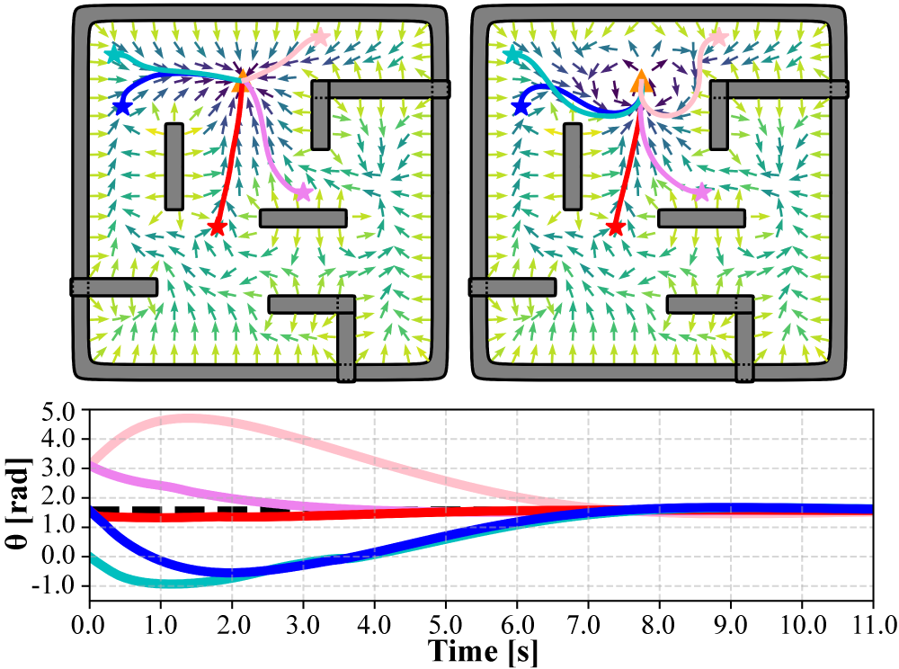
Figure 6: Robot trajectories from different initial poses (filled stars) to the same goal pose (orange triangle), under the original potential fields $-\nabla\varphi_{\texttt{NF}}(q)$ (Top Left) and the oriented potential fields $\Upsilon(q)$ (Top Right) via the proposed control law in (24). Bottom: The robot orientation $\theta$ converges to the desired value (dashed line), along these trajectories.

Two-step Rotation to Harmonic Potentials: As shown in Fig. 6, the main idea is to design a two-step rotation transformation to the harmonic potentials, such that a “dipole-like” field is formed near the goal point with the desired orientation. More specifically, the transformation is given by:

$$\Gamma(q)\triangleq\mathbf{R}\big{(}\theta_{2}(q)\big{)}\,\mathbf{R}\big{(}\theta_{1}(q)\big{)},$$ (20)

where $\mathbf{R}(\theta)$ is the standard rotation matrix, see e.g., LaValle (2006) associated with angle $\theta\in[0,-\pi)$, i.e.,

$$\mathbf{R}(\theta)\triangleq\begin{bmatrix}\cos\theta&-\sin\theta\\ \sin\theta&\ \ \cos\theta\end{bmatrix};$$

the variable $\theta_{1}(q)$ is the angle to be rotated such that the direction of the transformed potential fields is aligned with the direction from $q_{G}$ to $q$ near the goal, i.e.,

$$\theta_{1}(q)\triangleq s_{d}(q)\delta_{\theta}(q)+\mathbf{sgn}\big{(}\delta_{\theta}(q)\big{)}[1-s_{d}(q)]\delta_{c},$$ (21)

where $\delta_{\theta}(q)\triangleq\theta_{q-q_{G}}-\theta_{\nabla\varphi_{\texttt{NF}}(q)}$ is the relative angle between $q-q_{G}$ and $\nabla\varphi_{\texttt{NF}}(q)$; $\delta_{c}\triangleq 2\pi$; $s_{d}(q)\triangleq\exp{(\tau-\frac{\tau{\color[rgb]{0,0,0}\mu^{2}}}{(\mu-\varphi_{\texttt{NF}}(q))^{2}})}$ is a smooth switch function that is “on” near the destination and “off” near the obstacle, with $\tau\in(0,1)$ being a design parameter and $\mu$ being the maximum value of $\varphi_{\texttt{NF}}(q)$. Moreover, the variable $\theta_{2}(q)$ is the angle to be rotated, such that the transitional potential fields mimic a point-dipole field, i.e.,

$$\theta_{2}(\check{q})\triangleq s_{d}(\check{q})\delta^{\prime}_{\theta}(\check{q})+\mathbf{sgn}\big{(}\delta^{\prime}_{\theta}(\check{q})\big{)}[1-s_{d}(\check{q})]\delta^{\prime}_{c}+\delta^{\prime}_{c},$$ (22)

where $\check{q}$ is the transformed coordinate of $q$ in the new coordinate system, where the goal point $q_{G}$ is the origin and the desired orientation $\theta_{G}$ is the positive direction of the $x$-axis, i.e., $\check{q}\triangleq\mathbf{R}^{-1}(\theta_{G})(q-q_{G})$, where $\mathbf{R}(\theta_{G})$ is the rotation matrix associated with the goal angle $\theta_{G}$; $\delta^{\prime}_{\theta}(\check{q})\triangleq\theta_{\check{q}}$ is the angle of the vector $\check{q}$; $\delta^{\prime}_{c}\triangleq\pi$; $s_{d}(\cdot)$ is the same as in (21).

Definition 3.

The oriented harmonic potential fields are defined as the fields obtained by transforming the original potential fields through a two-step rotation in (20), denoted by:

$$\Upsilon(q)\triangleq-\Gamma(q)\nabla\varphi_{\texttt{NF}}(q),$$ (23)

where $\nabla\varphi_{\texttt{NF}}(q)$ is the gradient of the original potentials. $\blacksquare$

Given the oriented harmonic potential fields, the integral curves of $\Upsilon(q)$ correspond to the trajectories $\bar{\xi}(t)$ of the autonomous system described by ordinary differential equations: $\frac{d}{d\,t}\bar{\xi}(t)=\Upsilon(\bar{\xi}(t))\in\mathbb{R}^{2}$, with initial value $\bar{\xi}(t_{0})=q_{0}$. The convergence property of the integral curves is proven as follows.

Lemma 4.

All integral curves of $\Upsilon(q)$ in (23) converge to $q_{G}$ with the desired orientation $\theta_{G}$ asymptotically, with no collision with any obstacles, as long as the conditions in Lemma 3 hold.

Proof.

To begin with, it is proven in Lemma 3 that $\varphi_{\texttt{NF}}(q)$ is a valid navigation function, it holds that $\varphi_{\texttt{NF}}(q)=\mu$ on the boundary of the workspace $\partial\mathcal{W}$. Thus, the switch functions $s_{d}(q)=1$ hold both in (21) and (22), and $\theta_{1}(q)=\theta_{2}(q)=\pi$ holds. In this case, the rotation matrices $\mathbf{R}(\theta_{1})=\mathbf{R}(\theta_{2})$ are both identity matrices, thus $\Gamma(q)=\mathbf{I}$ is an identical transformation and the transformed field coincides with the original potential field, i.e., $-\nabla\varphi_{\texttt{NF}}(q)$. Furthermore, since the negated gradient points away from the boundary $\partial\mathcal{W}$, the transformed field inherits the property of collision avoidance.

Secondly, the transformation $\Gamma(q)$ is nonsingular as both $\mathbf{R}(\theta_{1})$ and $\mathbf{R}(\theta_{2})$ are non-singular. Thus, all critical points of $\varphi_{\texttt{NF}}(q)$, including the global minimum $q_{G}$ and saddle points, retain their properties after the transformation. In other words, the saddle points of $\varphi_{\texttt{NF}}(q)$ remain to be non-degenerate with an attraction region of measure zero. Since any integral curve in a closed compact set $\overline{\mathcal{W}}$ is bounded, there must be a limit set inside $\overline{\mathcal{W}}$ to which the integral curves converge. Lemma $4$ of Valbuena & Tanner (2012) states that no such limit cycles exist if there are no additional attractors other than $q_{G}$. Therefore, the goal point $q_{G}$ is the only attractive component of the limit set within $\overline{\mathcal{W}}$, i.e., the integral curves of $\Upsilon(q)$ converge to $q_{G}$.

Lastly, it remains to be shown that the asymptotic convergence to $q_{G}$ is achieved with the desired orientation $\theta_{G}$. Clearly, when $q$ approaches $q_{G}$, the switch function $s_{d}(q,\tau)$ approaches $1$, while $\theta_{1}(q),\theta_{2}(q)$ approach ${\delta}_{\theta}(q),\delta^{\prime}_{\theta}(q)+\pi$, respectively. For brevity, let $\theta_{1}(q)={\delta}_{\theta}(q)$ and $\theta_{2}(q)=\delta^{\prime}_{\theta}(q)+\pi$. Therefore, the transformed potential field $\Upsilon(q)$ is simplified as:

$$\Upsilon(q)=\begin{bmatrix}\|\nabla\varphi_{\texttt{NF}}(q)\|\cos\big{(}\delta^{\prime}_{\theta}(q)+\theta_{q-q_{G}}\big{)}\\ \|\nabla\varphi_{\texttt{NF}}(q)\|\sin\big{(}\delta^{\prime}_{\theta}(q)+\theta_{q-q_{G}}\big{)}\end{bmatrix},$$

where $\delta^{\prime}_{\theta}(q)\in(-\pi,\pi]$ is defined in (22). Then, the inner product of $\Upsilon(q)$ and $q_{G}-q$ is given by: $\langle\Upsilon(q),\ q_{G}-q\rangle=-\|\nabla\varphi_{\texttt{NF}}(q)\|\|q_{G}-q\|\cos\big{(}\delta^{\prime}_{\theta}(q)\big{)}$. It should be noted that the integral curves can only converge to the $q_{G}$ in the direction of steepest descent, i.e., from the region where $\delta^{\prime}_{\theta}(q)$ approaches $\pi$. Since $\delta^{\prime}_{\theta}(q)=\theta_{\check{q}}$ and $\check{q}=\mathbf{R}^{-1}(\theta_{G})(q-q_{G})$, $\delta^{\prime}_{\theta}(q)$ approaches $\pi$ implies that $\theta_{q_{G}-q}$ approaches $\theta_{G}$. Thus, the integral curves converge to $q_{G}$ along the desired orientation $\theta_{G}$. ∎

Remark 5.

Many existing navigation functions in Rousseas et al. (2021, 2022b); Filippidis & Kyriakopoulos (2011); Loizou & Rimon (2022, 2021) are globally convergent, but do not take into account the desired orientation at the goal point. Similar idea of rotating the gradients is adopted in Valbuena & Tanner (2012), but it requires that the goal orientation is aligned with the positive direction of $x$-axis, thus yielding a more restrictive approach than the two-step rotation in (20). $\blacksquare$

4.1.3 Smooth Harmonic-Tracking Controller

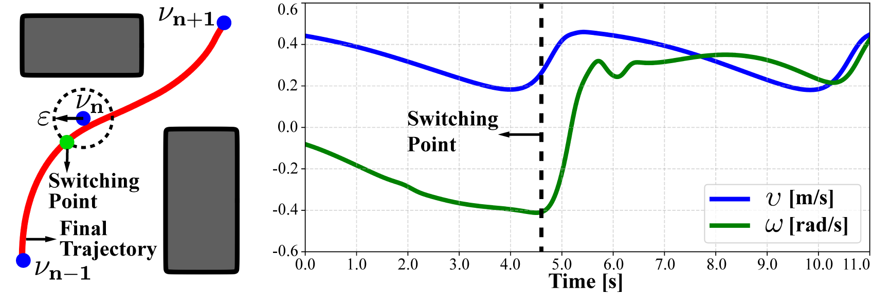
Figure 7: Illustration of the smooth transition strategy in (25) when the agent switches from one intermediate waypoint to another. The switch function $\eta_{\epsilon}$ is activated once the current waypoint is reached with a margin $\epsilon$. The resulting trajectory and control inputs are all smooth.

Given the rotated potentials in (23), a nonlinear feedback controller can be used for non-holonomic robots in (3) to track its rotated and negated gradient. More specifically, the linear and angular velocity is set as follows:

$$\upsilon(q,\,q_{G}) =k_{\upsilon}\,\tanh\left(\|q-q_{G}\|\right);$$ (24a)

$$\omega(\theta,\,\theta_{G}) =-k_{\omega}\left(\theta-\theta_{\Upsilon}\right)+\upsilon\,[\nabla\theta_{\Upsilon}]^{\intercal}\,J_{\Upsilon}\,\Theta,$$ (24b)

where $q,\,\theta$ are the robot pose and orientation; $k_{\upsilon},\,k_{\omega}>0$ are controller gains; $\theta_{\Upsilon}$ is the direction of vector $\Upsilon\triangleq[\Upsilon_{x},\,\Upsilon_{y}]^{\intercal}$; $\nabla\theta_{\Upsilon}=[\frac{\partial\,\theta_{\Upsilon}}{\partial\,\Upsilon_{x}},\,\frac{\partial\,\theta_{\Upsilon}}{\partial\,\Upsilon_{y}}]^{\intercal}$; $J_{\Upsilon}$ being the $2\times 2$ Jacobian matrix of $\Upsilon$, whose entries are $[J_{\Upsilon}]_{ij}=\frac{\partial\Upsilon_{i}}{\partial q_{j}}$, for $i,j\in\{1,2\}$; and $\Theta\triangleq[\cos\theta,\,\sin\theta]^{\intercal}$. The main idea is to decompose the control objective into two sub-objectives: (i) the robot orientation is regulated sufficiently fast to $\theta_{\Upsilon}$ via (24b); (ii) the robot velocity along this direction is adjusted to reach $q_{G}$ via (24a).

Proposition 1.

Under the control law (24), the robot in (3) converges to the goal $q_{G}$ with orientation $\theta_{G}$ asymptotically, from almost all initial poses in the workspace $\mathcal{W}$, as long as the conditions in Lemma 3 hold.

Proof.

(Sketch) As discussed, the robot system (3) under control law (24) can be decomposed into two subsystems via singular perturbation based on Khalil (2002). The fast subsystem is equivalent to $\omega=-k_{\omega}\left(\theta-\theta_{\Upsilon}\right)+\dot{\theta}_{\Upsilon}$, which ensures a global exponential convergence of $\theta$ to the rotated fields $\theta_{\Upsilon}$. Secondly, the slow subsystem is given by $\dot{q}=\upsilon\frac{\Upsilon}{\|\Upsilon\|}$. The robot trajectory corresponds one integral curve of the vector field $\Upsilon(q)$. As already proven in Lemma 3 that the integral curves of the vector fields $\Upsilon(q)$ converge to $q_{G}$ with orientation $\theta_{G}$, the slow subsystem converges to the goal pose with the desired orientation. ∎

More importantly, since the robot needs to switch along a sequence of waypoints in its path $\mathbf{P}_{\widehat{g}_{\ell}\rightarrow\widehat{g}_{\ell+1}}$ from (7), a smooth transition between the intermediate waypoints is crucial to ensure both smooth trajectories and control inputs. As shown in Fig. 7, the switching strategy from $\nu_{n}=(q_{n},\theta_{n})$ to $\nu_{n+1}=(q_{n+1},\theta_{n+1})$ in $\mathbf{P}_{\widehat{g}_{\ell}\rightarrow\widehat{g}_{\ell+1}}$ is given by:

$$u=u(q,\,q_{n})+\eta_{\varepsilon}\left(\gamma_{n}(q)\right)\,\big{(}u(q,\,q_{n+1})-u(q,\,q_{n})\big{)},$$ (25)

where $u$ stands for inputs $\upsilon$ and $\omega$; $\gamma_{n}(q)\triangleq\|q-q_{n}\|$; and $\eta_{\varepsilon}(x)\triangleq\frac{1}{2}\big{(}1+\tanh(k_{s}\,(\varepsilon-\gamma_{n}(q)))\big{)}$ is the smooth switch function, with $k_{s}>0$ being a positive gain, and $\varepsilon>0$ the switching margin around $q_{n}$. Last but not least, the control cost under the proposed control law in (24) to drive the robot from waypoint $\nu_{n}$ to $\nu_{n+1}$ is estimated by:

$$\gamma(\nu_{n},\,\nu_{n+1})\triangleq d(q_{n},\,q_{n+1})+\mathbf{w}\,{Q}_{\Upsilon}^{\intercal}(\theta_{n},\theta_{n+1}),$$ (26)

where the first part $d(q_{n},\,q_{n+1})=\|q_{n}-q_{n+1}\|$ measures the straight-line distance; the second part approximates the rotation cost: (i) $\mathbf{w}\triangleq[w_{1},w_{2}]$ are the weighting parameters with $w_{1},w_{2}$ $>0$; (ii) ${Q}_{\Upsilon}(\theta_{n},\theta_{n+1})\triangleq[|\theta_{\Upsilon(q_{n})}-\theta_{n}|,\,|\theta_{q_{n+1}-q_{n}}-\theta_{n+1}|]$, where the first item estimates the rotation cost between robot orientation and the rotated gradient at the starting pose; the second item estimates the steering cost between the vector $q_{n+1}-q_{n}$ and goal orientation. Consequently, it can be used to compute the edge cost of the HT $\mathcal{T}_{\widehat{g}_{\ell}\rightarrow\widehat{g}_{\ell+1}}$ in (6), yielding a more accurate estimate of the navigation cost from $\widehat{g}_{\ell}$ to $\widehat{g}_{\ell+1}$. In turn, the actual cost within the navigation map $\mathcal{G}$ is given by:

$$d(\widehat{g},\,\widehat{g}^{\prime})=\sum^{N-1}_{n=0}\gamma(\nu_{n},\,\nu_{n+1}),$$ (27)

where $\mathbf{P}_{\widehat{g}\rightarrow\widehat{g}^{\prime}}=\nu_{0}\nu_{1}\cdots\nu_{N}$ is the shortest path from $\widehat{g}$ to $\widehat{g}^{\prime}$ in the associated HT $\mathcal{T}_{\widehat{g}\rightarrow\widehat{g}^{\prime}}$.

Remark 6.

The control cost in (26) is estimated through a weighted combination of the translation cost and the steering cost. As shown in Fig. 8, this estimation approaches the actual measured cost when the distance between consecutive waypoints are selected properly. $\blacksquare$

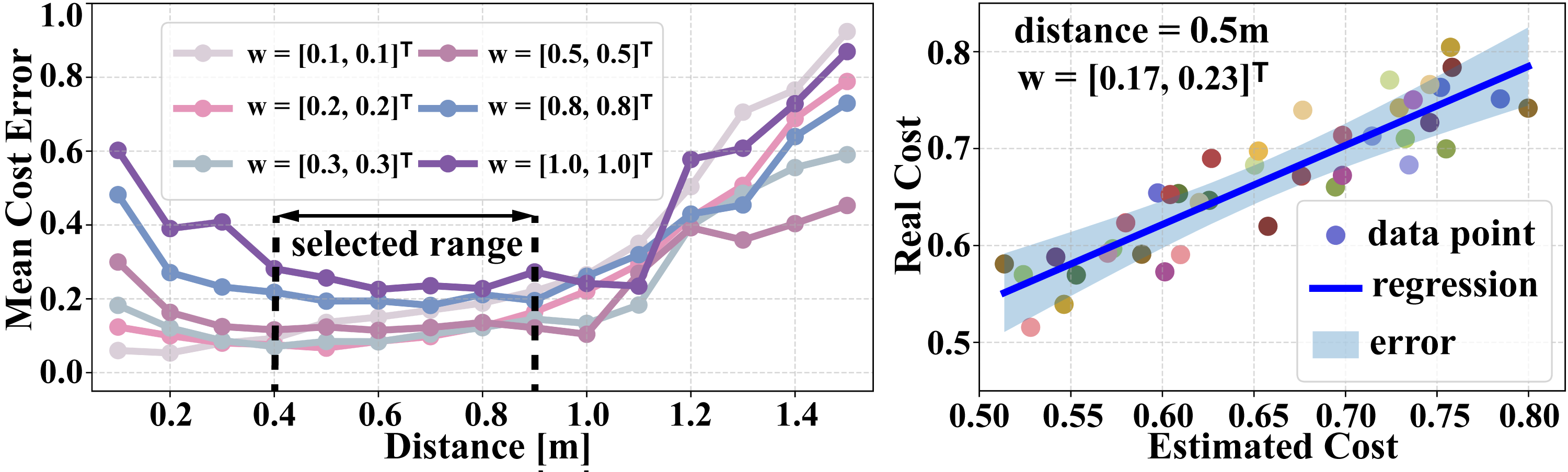
Figure 8: Left: The difference between the estimated cost by (26) and the measured cost under different weights $\mathbf{w}$, for different choice of the distance $d(q_{n},\,q_{n+1})$. Right: The difference actual with $40$ samples, when $\mathbf{w}=[0.17,\,0.23]^{\intercal}$ and $d=0.5$.

4.1.4 Hybrid Execution of the Initial Plan

The initial plan $\widehat{\mathbf{g}}=\widehat{g}_{1}\widehat{g}_{2}\cdots\widehat{g}_{L}(\widehat{g}_{L+1}\widehat{g}_{L+2}\cdots\widehat{g}_{L+H})^{\omega}$ in (5) can be executed via the following hybrid strategy: (i) staring from $\ell=1$, determine the next goal region $\widehat{g}_{\ell+1}$; (ii) construct the HT as $\mathcal{T}_{\widehat{g}_{\ell}\rightarrow\widehat{g}_{\ell+1}}$ and determine the shortest path $\mathbf{P}_{\widehat{g}_{\ell}\rightarrow\widehat{g}_{\ell+1}}=\nu_{0}\cdots\nu_{N-1}\nu_{G}$ in (7); (iii) starting from the first vertex $n=0$, once the robot enters the small vicinity of vertex $\nu_{n}$, it switches to the next mode of traversing the subsequent intermediate edge $(\nu_{n},\,\nu_{n+1})$. The associated controller (24) is activated with the goal pose $\nu_{n+1}$ and potential $\Upsilon_{\nu_{n}\rightarrow\nu_{n+1}}(q)$. The controller remains active until the robot enters the small vicinity of $\nu_{n+1}$. This execution repeats until the vertex $\nu_{G}$, i.e., $\widehat{g}_{\ell+1}$, is reached, after which the index $\ell$ is incremented by $1$ and returns to step (i). This procedure could be repeated until the last state of plan suffix $\hat{s}_{L+H}$ is reached, if the environment remains static. However, since the environment is only partially known, more obstacles would be detected during execution and added to the environment model. which might invalidate not only the current navigation map but also the underlying harmonic potentials.

Remark 7.

The design of intermediate waypoints between subtasks can alleviate certain limitations of the classic navigation functions from Koditschek (1987); Rimon (1990) for robotic navigation. As shown in Fig. 9, when the robotic system is geometrically and dynamically constrained, it can not follow the negated gradient perfectly. Consequently, oscillations appear along narrow passages and close to boundary of obstacles, where the underlying gradient changes directions abruptly. As also emphasized in Rimon (1990); Loizou & Rimon (2022), the phenomenon of “vanishing” valleys and the resulting oscillations often occur when the parameter $\lambda$ is set too large. Moreover, when two initial poses are located close to saddle points, the resulting trajectories can be diverging in opposite directions. To overcome these issues, the introduced intermediate waypoints can decompose the long path into shorter segments of which the associated potentials are often easier to track. $\blacksquare$

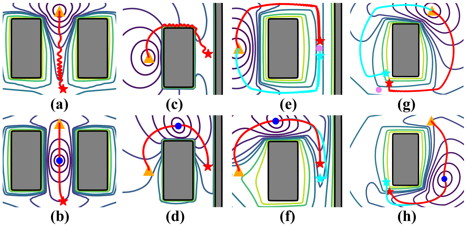
Figure 9: Illustration of how intermediate waypoints can reduce oscillations and long detours, under different initial poses (solid stars) and goal poses (orange triangles). (I) Oscillations appear as the robot traverses narrow passage in (a) or near the obstacle boundary in (c). Intermediate waypoints (blue dots) are introduced in (b) and (d), yielding smooth trajectories. (II) Divergent trajectories appear for two close-by initial poses (red and green stars) due to their proximity to the saddle point (violet dot) in (e) and (g). Intermediate waypoints (blue dots) are introduced in (f) and (h), yielding nearly identical trajectories.

4.2 Online Adaptation

As the robot detects more obstacles during execution, both the HTs and the underlying harmonic potentials should be updated. Total re-computation of both parts whenever a new obstacle is detected would require significant computational resources, yielding it unsuitable for online real-time applications. Instead, recursive algorithms are proposed here to incrementally update the harmonic potentials and tree structures.

4.2.1 Incremental Update of Harmonic Potentials

The classic methods as proposed in Loizou & Rimon (2022); Li & Tanner (2018); Rimon (1990) construct the underlying navigation function at once by taking into account all obstacles in the workspace. However, this means that the whole process has to be repeated from scratch each time an additional obstacle is added. A more intuitive approach would be to incrementally update different parts of the computation process by storing and re-using some of the intermediate results. Consider the following two cases as shown in Fig. 10: (i) independent stars are added to existing world of stars; and (ii) overlapping stars are added to existing forests of stars.

Independent Stars: To begin with, consider the simple case that a set of non-overlapping star obstacles, denoted by $\mathcal{O}_{k}$, $k=1,\cdots,M$, is added to an empty workspace $\mathcal{W}=\mathcal{O}_{0}$ in sequence. As discussed in Sec. 4.1.2, the star-to-sphere transformation for each obstacle is constructed via the translated scaling map in (11). Specifically, the transformation from star world to sphere world after adding the $k$-th star is restated as:

$$\Phi_{\mathcal{S}\rightarrow\mathcal{M}}^{k}(q)\triangleq{\rm id}(q)+\sum_{i=0}^{k}s_{i}^{k}(q)\,\big{(}v_{i}(q)-1\big{)}\,(q-q_{i}),$$ (28)

where $s_{i}^{k}(q)$ is the online analytic switch associated with both $i$ and $k$; $v_{i}(q)$ is the scaling factor defined in (10); and $q_{i}$ is the geometric center of the obstacle $\mathcal{O}_{i}$, for $i=0,1,\cdots,k$.

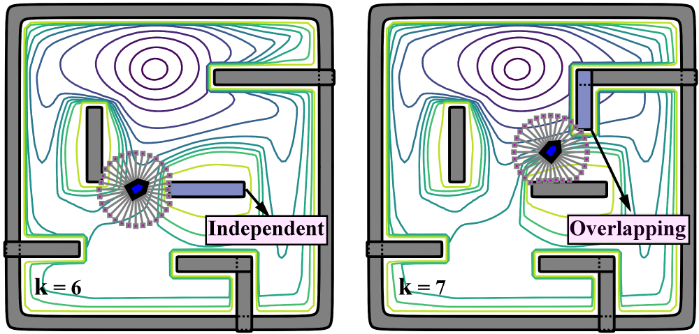
Figure 10: Iterative update of the harmonic potentials as new obstacles are detected and added into the workspace. An independent obstacle is added for $k=6$ (Left), while an overlapping obstacle is added for $k=7$ (Right).

Definition 4.

The online omitted product $\overline{\beta}_{i}^{k}(q)$ of star-to-sphere transformation for obstacle $\mathcal{O}_{i}$ after adding the $k$-th obstacle, for $i=0,1,\cdots,k$ and for $k=1,\cdots,M$, is a real-valued function defined for the star world $\mathcal{S}$ as: $\overline{\beta}_{i}^{k}(q)\triangleq\prod_{j=0,j\neq i}^{k}\beta_{j}(q)$, where $\beta_{j}(q)$ is the obstacle function defined in (8). $\blacksquare$

Definition 5.

The online analytic switch $s_{i}^{k}(q)$ of star-to-sphere transformation for obstacle $\mathcal{O}_{i}$, after adding the $k$-th obstacle, for $i=0,1,\cdots,k$ and for $k=1,\cdots,M$, is a real-valued function defined for a star world $\mathcal{S}$ as:

$$s_{i}^{k}(q)\triangleq\frac{\gamma_{G}(q)\overline{\beta}_{i}^{k}(q)}{\lambda_{k}\beta_{i}(q)+\gamma_{G}(q)\overline{\beta}_{i}^{k}(q)},$$

where $\gamma_{G}(q)$ is the distance-to-goal function; $\lambda_{k}$ is a positive parameter associated with $k$; $\overline{\beta}_{i}^{k}(q)$ is the online omitted product; and $\beta_{i}(q)$ is the obstacle function defined in (8). $\blacksquare$

Then, the following intermediate variables are defined:

$$\mathbf{F}_{i}^{k}(q)\triangleq s_{i}^{k}(q)\,\mathbf{r}_{i}(q),$$ (29)

where $\mathbf{r}_{i}\triangleq\big{(}v_{i}(q)-1\big{)}(q-q_{i})$. Consequently, the transformation in (28) is adjusted to: $\Phi_{\mathcal{S}\rightarrow\mathcal{M}}^{k}(q)={\rm id}(q)+\sum_{i=0}^{k}\mathbf{F}_{i}^{k}(q)$. Note that for $k=0$, the function $\mathbf{F}_{0}^{0}(q)$ for the empty workspace is computed using the initial transformation via (12). Afterwards, each time a new $(k+1)$-th obstacle is added, $\mathbf{F}_{i}^{k}(q)$ should be updated to $\mathbf{F}_{i}^{k+1}(q)$, $\forall i=0,1,\cdots,k$, and $\mathbf{F}_{k+1}^{k+1}(q)$ for the added obstacle should also be constructed. To compute these variables efficiently, a recursive method is proposed here. For the ease of notation, define the multi-variate auxiliary function useful for the recursive computation as follows:

$$\Psi_{\texttt{a}}(\mathbf{F},\,\mathbf{r},\,\mathbf{\tilde{r}},\,\alpha)\triangleq\frac{\|\mathbf{F}\|}{\alpha\,\|\mathbf{r}\|+(1-\alpha)\,\|\mathbf{F}\|}\,\mathbf{\tilde{r}},$$ (30)

where $\mathbf{F},\mathbf{r},\mathbf{\tilde{r}}$ are vectors; $\alpha\in(0,\,1)$ is a scalar variable; and $\alpha\,\|\mathbf{r}\|+(1-\alpha)\,\|\mathbf{F}\|\neq 0$. Then, the function $\mathbf{F}_{0}^{k+1}(q)$ associated with the workspace is updated from $\mathbf{F}_{0}^{k}(q)$ as follows:

$$\mathbf{F}_{0}^{k+1}(q)=\Psi_{\texttt{a}}\left(\mathbf{F}_{0}^{k}(q),\,\mathbf{r}_{0}(q),\,\mathbf{r}_{0}(q),\,\alpha^{k}(q)\right),$$ (31)

where $\mathbf{r}_{0}(q)$ is defined in (29) for the workspace; the variable $\alpha^{k}(q)\triangleq\lambda_{k+1}/\big{(}\lambda_{k}\,\beta_{k+1}(q)\big{)}$; $\lambda_{k}$ and $\lambda_{k+1}$ are positive parameters defined in (5), for $k=0,1,\cdots,M$.

Lemma 5.

Each time an independent obstacle $\mathcal{O}_{k+1}$ is added to the workspace, the following holds:

(i) the online omitted product for $\mathcal{O}_{0}$ is given by $\overline{\beta}_{0}^{k+1}(q)=\overline{\beta}_{0}^{k}(q)\,\beta_{k+1}(q)$;

(ii) the online analytic switch for $\mathcal{O}_{0}$ is given by $s_{0}^{k+1}(q)=\frac{s_{0}^{k}(q)}{\alpha^{k}(q)\,(1-s_{0}^{k}(q))+s_{0}^{k}(q)}$, where $\alpha^{k}(q)=\lambda_{k+1}/\big{(}\lambda_{k}\,\beta_{k+1}(q)\big{)}$.

Proof.

(Omitted) Available in the supplementary files. ∎

Proposition 2.

Each time an independent obstacle $\mathcal{O}_{k+1}$ is added to the workspace, the recursive calculation of $\mathbf{F}_{0}^{k+1}(q)$ in (31) for $\mathcal{O}_{0}$ is valid for iteration $k=0,1,\cdots,M-1$.

Proof.

(Sketch) The proof is done by induction. Namely, the initial value of $\mathbf{F}_{0}^{k}(q)$ is given by $\mathbf{F}_{0}^{0}(q)=s_{0}^{0}(q)\,\mathbf{r}_{0}(q)$ with $s_{0}^{0}(q)=\frac{\gamma_{G}(q)}{\lambda_{0}\beta_{0}(q)+\gamma_{G}(q)}$, which satisfies (29). Now assume that $\mathbf{F}_{0}^{\ell}(q)=s_{0}^{\ell}(q)\,\mathbf{r}_{0}(q)$ and $s_{0}^{\ell}(q)=\frac{\gamma_{G}(q)\overline{\beta}_{0}^{\ell}(q)}{\lambda_{\ell}\beta_{0}(q)+\gamma_{G}(q)\overline{\beta}_{0}^{\ell}(q)}$ hold for an integer $\ell\geq 0$. Then, $\mathbf{F}_{0}^{\ell+1}(q)$ is derived via (31) as:

$$\mathbf{F}_{0}^{\ell+1}(q)=\frac{\|s_{0}^{\ell}(q)\,\mathbf{r}_{0}(q)\|\,\mathbf{r}_{0}(q)}{\alpha^{\ell}(q)\,\|\mathbf{r}_{0}(q)\|+\big{(}1-\alpha^{\ell}(q)\big{)}\,\|s_{0}^{\ell}(q)\,\mathbf{r}_{0}(q)\|}.$$

Given (8), it holds that $\beta_{0}(q)\geq 0$ and $\overline{\beta}_{0}^{\ell}(q)\geq 0$, which implies that $s_{0}^{\ell}(q)\in[0,\,1]$. Therefore, $\mathbf{F}_{0}^{\ell+1}(q)$ is simplified as $\mathbf{F}_{0}^{\ell+1}(q)=\frac{s_{0}^{\ell}(q)\,\mathbf{r}_{0}(q)}{\alpha^{\ell}(q)+(1-\alpha^{\ell}(q))\,s_{0}^{\ell}(q)}$ Further, Lemma 5 implies that $s_{0}^{\ell}(q)=\frac{\alpha^{\ell}(q)\,s_{0}^{\ell+1}(q)}{(\alpha^{\ell}(q)-1)\,s_{0}^{\ell+1}(q)+1}$. Combined with $\mathbf{F}_{0}^{\ell+1}(q)$, it yields that $\mathbf{F}_{0}^{\ell+1}(q)=s_{0}^{\ell+1}(q)\,\mathbf{r}_{0}(q),$ which is consistent with (29), thus concluding the proof. ∎

Furthermore, the function $\mathbf{F}_{i+1}^{k+1}(q)$ for each inner obstacle $i=0,1,\cdots,k$ is calculated from $\mathbf{F}_{0}^{k+1}(q)$ iteratively by:

$$\mathbf{F}_{i+1}^{k+1}(q)=\Psi_{\texttt{a}}\left(\mathbf{F}_{i}^{k+1}(q),\,\mathbf{r}_{i}(q),\,\mathbf{r}_{i+1}(q),\,\alpha_{i}(q)\right),$$ (32)

where $\mathbf{r}_{i}(q)$ and $\mathbf{r}_{i+1}(q)$ are defined in (29) for the $i$-th and $(i+1)$-th obstacles; $\alpha_{i}(q)=(\beta_{i+1}(q))^{2}/(\beta_{i}(q))^{2}$.

Lemma 6.

Each time an independent obstacle $\mathcal{O}_{k+1}$ is added to the workspace, the following holds:

(i) the online omitted product for $\mathcal{O}_{i+1}$ is given by $\overline{\beta}_{i+1}^{k+1}(q)=\overline{\beta}_{i}^{k+1}(q)\,\frac{\beta_{i}(q)}{\beta_{i+1}(q)}$;

(ii) the online analytic switch for $\mathcal{O}_{i+1}$ is given by $s_{i+1}^{k+1}(q)=\frac{s_{i}^{k+1}(q)}{\alpha_{i}(q)\,(1-s_{i}^{k+1}(q))+s_{i}^{k+1}(q)}$, where $\alpha_{i}(q)=(\beta_{i+1}(q))^{2}/(\beta_{i}(q))^{2}$.

Proof.

(Omitted) Available in the supplementary files. ∎

Proposition 3.

Each time an independent obstacle $\mathcal{O}_{k+1}$ is added to the workspace, the recursive calculation of $\mathbf{F}_{i+1}^{k+1}(q)$ in (31) for $\mathcal{O}_{i+1}$ is valid for iteration $i=0,1,\cdots,k$.

Proof.

(Sketch) Similar to Proposition 2, the proof is done by induction. The initial value of $\mathbf{F}_{i}^{k+1}(q)$ is given by $\mathbf{F}_{0}^{k+1}(q)=s_{0}^{k+1}(q)\,\mathbf{r}_{0}(q)$, which fulfills (29). Now assume that $\mathbf{F}_{\ell}^{k+1}(q)=s_{\ell}^{k+1}(q)\,\mathbf{r}_{\ell}(q)$ with $s_{\ell}^{k+1}(q)=\frac{\gamma_{G}(q)\overline{\beta}_{\ell}^{k+1}(q)}{\gamma_{G}(q)\overline{\beta}_{\ell}^{k+1}(q)+\lambda_{k+1}\beta_{\ell}(q)}$ holds for an integer $\ell\geq 0$. Then, $\mathbf{F}_{\ell+1}^{k+1}(q)$ is derived via (31) as:

$$\mathbf{F}_{\ell+1}^{k+1}(q)=\frac{\|s_{\ell}^{k+1}(q)\,\mathbf{r}_{\ell}(q)\|\,\mathbf{r}_{\ell+1}(q)}{\alpha_{\ell}(q)\,\|\mathbf{r}_{\ell}(q)\|+\big{(}1-\alpha_{\ell}(q)\big{)}\,\|s_{\ell}^{k+1}(q)\,\mathbf{r}_{\ell}(q)\|}.$$

Since $s_{\ell}^{k+1}(q)\in[0,1]$ holds, it can be simplified to $\mathbf{F}_{\ell+1}^{k+1}(q)=\frac{s_{\ell}^{k+1}(q)\,\mathbf{r}_{\ell+1}(q)}{\alpha_{\ell}(q)\,+(1-\alpha_{\ell}(q))\,s_{\ell}^{k+1}(q)}$. Furthermore, Lemma 6 implies that $s_{\ell}^{k+1}(q)=\frac{s_{\ell+1}^{k+1}(q)}{\alpha_{\ell}(q)\,(1-s_{\ell+1}^{k+1}(q))+s_{\ell+1}^{k+1}(q)}$. Combined with $\mathbf{F}_{\ell+1}^{k+1}(q)$, it yields that $\mathbf{F}_{\ell+1}^{k+1}(q)=s_{\ell+1}^{k+1}(q)\,\mathbf{r}_{\ell+1}(q),$ which is consistent with (29), thus concluding the proof. ∎

Remark 8.

Note that $\mathbf{F}_{0}^{k+1}(q)$ in (31) is iterated over the index $k$ with initial value $\mathbf{F}^{0}_{0}(q)$ while $\mathbf{F}_{i+1}^{k+1}(q)$ in (32) is iterated over the index $i$ with initial value $\mathbf{F}_{0}^{k+1}(q)$. The reason is that as the $(k+1)$-th obstacle is added to the existing star world, $\mathbf{F}_{0}^{k}$ for the outer boundary should be updated to $\mathbf{F}_{0}^{k+1}$ first, and then the transformation $\mathbf{F}_{i+1}^{k+1}$ for each inner obstacle $i=0,1,\cdots,k$ is constructed incrementally based on $\mathbf{F}_{0}^{k+1}$. $\blacksquare$

Overlapping Stars: Secondly, it is also possible that the new obstacle is overlapping with an existing obstacle. More precisely, assume that a sequence of star obstacles, denoted by $\{\mathcal{O}_{k},k=1,\cdots,N\}$, is added to a star world and overlapping with one of the existing obstacles as a leaf. As discussed in Sec. 4.1.2 for the static scenario, the purging transformation (14) for the leaf obstacles is also constructed by ray scaling process(18). To be specific, the purging transformation for the $k$-th obstacle in one of the tree is restated as:

$$f_{k}(q)\triangleq{\rm id}(q)+\sigma_{k}(q)\,\big{(}v_{k}(q)-1\big{)}\,(q-p_{k}),$$ (33)

where $\sigma_{k}(q)$ is the online analytic switch associated with $k$; $v_{k}(q)$ is the scaling factor defined in (18); and $p_{k}$ is the common center between the obstacle $\mathcal{O}_{k}$ and its parent $\mathcal{O}_{k}^{\star}$.

Definition 6.

The online omitted product $\overline{\beta}_{k}(q)$ of leaf-purging transformation for obstacle $\mathcal{O}_{k}$, after adding the $k$-th obstacle for $k=1,\cdots,N$, is defined on the forest world $\mathcal{F}$ as:

$$\overline{\beta}_{k}(q)\triangleq\Big{(}\prod_{j=0,j\neq k^{\star}}^{k-1}\beta_{j}(q)\Big{)}\Big{(}\prod_{j\in\mathcal{L}\backslash\{k\}}\beta_{j}(q)\Big{)}\tilde{\beta}_{k}(q),$$ (34)

where $\tilde{\beta}_{k}(q)$ is defined in (19); $\beta_{j}(q)$ is the obstacle function defined in (8); and $\mathcal{L}$ is the set of indices for all leaves in $\mathcal{F}$. $\blacksquare$

Definition 7.

The online analytic switch $\sigma_{k}(q)$ of leaf-purging transformation for obstacle $\mathcal{O}_{k}$, after adding the $k$-th obstacle for $k=1,\cdots,N$, is defined on the forest world $\mathcal{F}$ as:

$$\sigma_{k}(q)\triangleq\frac{\gamma_{G}(q)\overline{\beta}_{k}(q)}{\xi_{k}\beta_{k}(q)+\gamma_{G}(q)\overline{\beta}_{k}(q)},$$ (35)

where $\gamma_{G}(q)$ is the distance-to-goal function; $\xi_{k}$ is a positive parameter associated with $k$; $\overline{\beta}_{k}(q)$ is the online omitted product; and $\beta_{k}(q)$ is the obstacle function. $\blacksquare$

Similar to (29), the intermediate variables are defined as:

$$\mathbf{H}_{k}(q)\triangleq\sigma_{k}(q)\,\mathbf{r}_{k}(q),$$ (36)

where $\mathbf{r}_{k}(q)\triangleq\big{(}v_{k}(q)-1\big{)}(q-p_{k})$. Consequently, the transformation from forest world to star world after adding the $k$-th star obstacle is given by:

$$\Phi_{\mathcal{F}\rightarrow\mathcal{S}}^{k}(q)\triangleq\mathbf{H}_{1}\circ\mathbf{H}\circ\cdots\circ\mathbf{H}_{k}(q).$$ (37)

Note that for $k=1$, the new obstacle forms a new tree of stars and the transformation function $\mathbf{H}_{1}(q)$ is computed via (19). Afterwards, each time a new $(k+1)$-th obstacle is added, the transformation (37) should be updated as follows:

$$\Phi_{\mathcal{F}\rightarrow\mathcal{S}}^{k+1}(q)=\Phi_{\mathcal{F}\rightarrow\mathcal{S}}^{k}\circ\mathbf{H}_{k+1}(q),$$ (38)

where $\mathbf{H}_{k+1}(q)$ is calculated from $\mathbf{H}_{k}(q)$ iteratively by:

$$\mathbf{H}_{k+1}(q)=\Psi_{\texttt{a}}\left(\mathbf{H}_{k}(q),\,\mathbf{r}_{k}(q),\,\mathbf{r}_{k+1}(q),\,\alpha_{k}(q)\right),$$ (39)

where $\Psi_{\texttt{a}}(\cdot)$ is defined in (30); $\mathbf{r}_{k+1}(q)$ and $\mathbf{r}_{k}(q)$ are defined in (36); and $\alpha_{k}(q)$ is another intermediate variable, given by:

$$\alpha_{k}(q)=\zeta_{k}\,\frac{\beta_{k+1}(q)\,\tilde{\beta}_{k}(q)\,\beta_{{(k+1)}^{\star}}(q)}{(\beta_{k}(q))^{3}\,\tilde{\beta}_{k+1}(q)\,\beta_{{k}^{\star}}(q)},$$

where $\zeta_{k}=\xi_{k+1}/\xi_{k}$ with $\xi_{k}$ and $\xi_{k+1}$ being the design parameters from (14); $\tilde{\beta}_{k+1}(q)$ and $\tilde{\beta}_{k}(q)$ are defined as in (19).

Lemma 7.

Each time an obstacle $\mathcal{O}_{k+1}$ is added to the workspa-ce and overlapping with an existing obstacle, the following holds:

(i) the online omitted product for $\mathcal{O}_{k+1}$ is given by $\overline{\beta}_{k+1}(q)=\overline{\beta}_{k}(q)\,\frac{(\beta_{k}(q))^{2}\,\tilde{\beta}_{k+1}(q)\,\beta_{{k}^{\star}}(q)}{\tilde{\beta}_{k}(q)\,\beta_{{(k+1)}^{\star}}(q)}$;

(ii) the online analytic switch for $\mathcal{O}_{k+1}$ is given by: $\sigma_{k+1}(q)=\frac{\sigma_{k}(q)}{\alpha_{k}(q)(1-\sigma_{k}(q))+\sigma_{k}(q)}$, where $\alpha_{k}(q)=\frac{\xi_{k+1}\,\beta_{k+1}(q)\,\tilde{\beta}_{k}(q)\,\beta_{{(k+1)}^{\star}}(q)}{\xi_{k}\,(\beta_{k}(q))^{3}\,\tilde{\beta}_{k+1}(q)\,\beta_{{k}^{\star}}(q)}$.

Proof.

(Omitted) Available in the supplementary files. ∎

Proposition 4.

Each time an obstacle $\mathcal{O}_{k+1}$ is added to the workspace and overlapping with an existing obstacle, the recursive calculation of $H_{k+1}(q)$ in (39) is valid, for each new leaf obstacle $k=0,1,\cdots,N-1$.

Proof.

Similar to Proposition 3, the proof is done by induction. The initial value of $\mathbf{H}_{k}(q)$ is given by $\mathbf{H}_{1}(q)=\sigma_{1}(q)\,\mathbf{r}_{1}(q)$, which satisfies (36). Assume that $\mathbf{H}_{\ell}(q)=\sigma_{\ell}(q)\,\mathbf{r}_{\ell}(q)$ with $\sigma_{\ell}(q)=\frac{\gamma_{G}(q)\overline{\beta}_{\ell}(q)}{\gamma_{G}(q)\overline{\beta}_{\ell}(q)+\xi_{k}\beta_{\ell}(q)}$ holds for an integer $\ell\geq 0$. Then, $\mathbf{H}_{\ell+1}(q)$ is computed via (39) as:

$$\mathbf{H}_{\ell+1}(q)=\frac{\|\sigma_{\ell}(q)\,\mathbf{r}_{\ell}(q)\|\,\mathbf{r}_{\ell+1}(q)}{\alpha_{\ell}(q)\,\|\mathbf{r}_{\ell}(q)\|+(1-\alpha_{\ell}(q))\,\|\sigma_{\ell}(q)\,\mathbf{r}_{\ell}(q)\|}.$$

Since $\sigma_{\ell}(q)\in[0,1]$, it holds that $\mathbf{H}_{\ell+1}(q)=\frac{\sigma_{\ell}(q)\,\mathbf{r}_{\ell+1}(q)}{\alpha_{\ell}(q)+(1-\alpha_{\ell}(q))\sigma_{\ell}(q)}$. When combined with $\sigma_{\ell}(q)=\frac{\sigma_{\ell+1}(q)}{\alpha_{\ell}(q)\,(1-\sigma_{\ell+1}(q))+\sigma_{\ell+1}(q)}$ from Lemma 7, $\mathbf{H}_{\ell+1}(q)=\sigma_{\ell+1}(q)\,\mathbf{r}_{\ell+1}(q)$ holds, which is consistent with (36), thus concluding the proof. ∎

Remark 9.

Note that the same auxiliary function $\Psi(\cdot)$ in (30) is used for the recursive computation in (31), (32) and (39). $\blacksquare$

Remark 10.

The parameters $\lambda_{k}$ in Def. 5 for $k=0,1,\cdots,M$, and $\xi_{k}$ in Def. 7 for $k=1,2,\cdots,N$ should satisfy the conditions in Lemma 3, i.e., $\lambda_{k}>\Lambda_{k}$ for some positive numbers $\Lambda_{k}>0$; and $\xi_{k}>\Xi_{k}$ for some positive numbers $\Xi_{k}>0$. $\blacksquare$

Combination of both cases: Overall, the above two cases can be summarized into a more general formula. Namely, the recursive transformation from forest of stars to sphere world after adding the $k$-th obstacle $\mathcal{O}_{k}$ is given by:

$$\Phi_{\mathcal{F}\rightarrow\mathcal{M}}^{k}(q)\triangleq\Phi_{\mathcal{S}\rightarrow\mathcal{M}}^{k}\circ\Phi_{\mathcal{F}\rightarrow\mathcal{S}}^{k}(q),$$ (40)

where if the new obstacle $\mathcal{O}_{k+1}$ is added to the workspace as an independent star, $\Phi_{\mathcal{S}\rightarrow\mathcal{M}}^{k}$ is updated to $\Phi_{\mathcal{S}\rightarrow\mathcal{M}}^{k+1}$ by (28); on the other hand, if the new obstacle $\mathcal{O}_{k+1}$ is overlapping with any existing obstacle, $\Phi_{\mathcal{F}\rightarrow\mathcal{S}}^{k}$ is updated to $\Phi_{\mathcal{F}\rightarrow\mathcal{S}}^{k+1}$ by (38). Moreover, each time an independent star $\mathcal{O}_{M+1}$ is added to the workspace, the complete harmonic potential function defined in point world should be updated by the recursive rule:

$$\phi_{\mathcal{P}}^{k+1}(x)=\frac{K}{K+1}\,\phi_{\mathcal{P}}^{k}(x)+\frac{1}{K+1}\big{(}\phi(x,\,P_{d})+\phi(x,P_{M+1})\big{)},$$

where $\phi_{\mathcal{P}}^{k}(x)$ and $\phi_{\mathcal{P}}^{k+1}(x)$ are the potential function in the $k$-th and $(k+1)$-th step; $\phi(x,P_{M+1})$ is the harmonic term for the new point obstacle. Given the updated transformation $\Phi_{\mathcal{F}\rightarrow\mathcal{M}}^{k+1}$ and the underlying harmonic potentials in point world $\phi_{\mathcal{P}}^{k+1}$, the new navigation function is adapted to $\varphi_{\texttt{NF}}^{k+1}$ accordingly.

4.2.2 Local Revision of Harmonic Trees

As new obstacles are detected, parts of some Oriented Harmonic Trees $\{\mathcal{T}_{\widehat{g}_{\ell}\rightarrow\widehat{g}_{\ell+1}}\}$ constructed in Sec. 4.1.1 might become invalid as the existing vertices might fall inside the new obstacle, and more importantly, the cost associated with certain edges should be recomputed as the underlying harmonic potentials are updated in Sec. 4.2.1. Instead of total reconstruction, this section describes how the Harmonic Trees and the resulting paths are revised incrementally as new obstacles are detected.

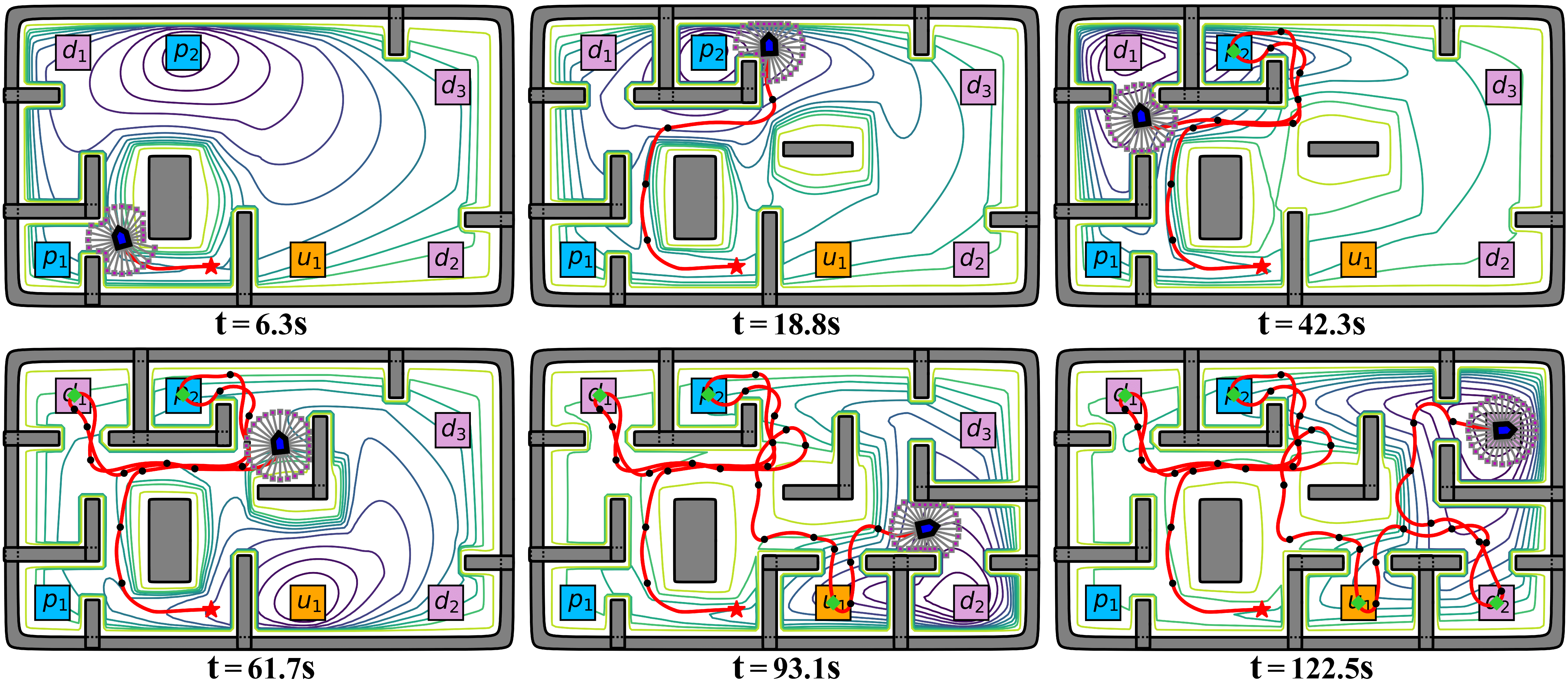
Figure 11: Snapshots of simulation when the high-level plan and the underlying harmonic potentials are updated, as the robot explores gradually the workspace. The robot trajectory is depicted in red; the task nodes in $\mathcal{G}$ are highlighted in green; and the intermediate waypoints in $\mathcal{T}$ are marked in black.

The revision procedure consists of three main steps: (I) Trimming of Harmonic trees. For each HT $\mathcal{T}_{\widehat{g}_{\ell}\rightarrow\widehat{g}_{\ell+1}}$, find the vertices that are within the newly-added obstacle, i.e., $\nu\in\mathcal{O}_{k}$, and remove them from the set of vertices $V$, along with the attached edges. As a result, the remaining tree might become disconnected and thus a path from its current vertex the goal might no longer exist; (II) Potential-biased regeneration. To re-connect the oriented HT to the goal vertex, new vertices and edges are generated. A process similar to the initial construction in Sec. 4.1.1 could be followed. However, depending on how the workspace has changed, it could be more efficient to focus the growth towards the obstacle areas that has been modified. Depending on the particular method of discretization, new vertices could be generated with the bias: $b(q)\;\propto\;|\zeta^{k+1}(q)-\zeta^{k}(q)|,$ where $b(q)$ is the probability of generating a new vertex at $q$; $\zeta^{k}(q)\triangleq\exp(1-\frac{1}{\varphi_{\texttt{NF}}^{k}(q)})$ and similarly for $\zeta^{k+1}(q)$; the right-hand side measures the relative change of the potential after adding obstacle $\mathcal{O}_{k+1}$. In other words, the harmonic tree are re-grown more towards the area with large change in its potential value; (III) Path revision. Once new vertices and edges are added, the associated edge costs should be re-evaluated by (27). Since numerous edges have been traversed during execution, their actual costs have been measured and saved. Consequently, the estimation model in (26) can be updated to approximate the transition cost more accurately. More specifically, suppose that at each time of update $H$ edges have been traversed in total, of which their actual costs are given by $\boldsymbol{\gamma}^{\star}=(\gamma_{1}^{\star},\cdots,\gamma_{H}^{\star})$. Their estimated costs are $\bar{\mathbf{\gamma}}=(\gamma_{1},\cdots,\gamma_{H})$ with $\bar{\mathbf{d}}$ and $\bar{\mathbf{Q}}$ being the distance and rotation cost respectively from (26). Then, the weighting parameters can be updated by: $\mathbf{w}^{\star}=(\bar{\mathbf{Q}}^{\intercal}\bar{\mathbf{Q}})^{-1}\bar{\mathbf{Q}}^{\intercal}$ $(\boldsymbol{\gamma}^{\star}-\bar{\mathbf{d}})$, which is then used to update all edge costs, even for other HTs. Afterwards, the revised path is found via the same search algorithm to the goal vertex.

4.2.3 Asymptotic Adaptation of Task Plan

On the highest level, since the HTs are updated, the associated feasibility and costs in the navigation map $\mathcal{G}$ should be updated accordingly, which in turn leads to a different task plan $\hat{\mathbf{g}}$. More specifically, the navigation map $\mathcal{G}$ is updated in two steps: (i) the feasibility of navigation from $\widehat{g}$ to $\widehat{g}^{\prime}$ in $\mathcal{G}$ is re-evaluated based on whether the path $\mathbf{P}_{\widehat{g}\rightarrow\widehat{g}^{\prime}}$ exists within the HT $\mathcal{T}_{\widehat{g}\rightarrow\widehat{g}^{\prime}}$. If not, the transition $(g,\,g^{\prime})$ is removed from the edge set $E$. This is often caused by newly-discovered obstacles blocking some passages; (ii) the costs of transitions within $E$ are re-computed by (27) given the updated path within the new HTs. Consequently, the navigation map $\mathcal{G}$ is up-to-date with the latest environment model. Thus, the task plan $\widehat{\mathbf{g}}^{\star}$ is re-synthesized within the updated product $\hat{\mathcal{A}}$ by searching for a path from the current product state to an accepting state. In other words, as the environment is gradually explored, the suffix of the task plan often would converge to optimal one asymptotically.

4.3 Summary and Complexity Analyses

To summarize, during the initial synthesis, the navigation map $\mathcal{G}$ is constructed hierarchically by building first the HTs $\{\mathcal{T}_{\widehat{g}\rightarrow\widehat{g}^{\prime}}\}$ associated with each transition of $\mathcal{G}$, and then the oriented Harmonic potentials $\{\Upsilon_{\nu\rightarrow\nu^{\prime}}\}$ associated with each edge of $\mathcal{T}_{\widehat{g}\rightarrow\widehat{g}^{\prime}}$. Given $\mathcal{G}$, the initial plan $\widehat{\mathbf{g}}$ is derived after computing the product automaton $\widehat{\mathcal{A}}$. Afterwards, the plan $\widehat{\mathbf{g}}$ is executed also hierarchically by tracing first the sequence of transitions and then the sequence of edges associated with each transition. Meanwhile, as the robot explores more obstacles, the harmonic potentials $\{\Upsilon\}$ are updated recursively, based on which the HTs $\{\mathcal{T}_{\widehat{g}\rightarrow\widehat{g}^{\prime}}\}$ and navigation map $\mathcal{G}$ are revised locally. Consequently, the task plan $\widehat{\mathbf{g}}$ is adapted given the current robot pose and the updated product automaton $\widehat{\mathcal{A}}$. This procedure continues indefinitely until termination.

The computational complexity to construct the product $\widehat{\mathcal{A}}$ is $\mathcal{O}(|G|^{2}|\mathcal{A}_{\varphi}|^{2})$, where $|G|$ is the number of goal regions and $|\mathcal{A}_{\varphi}|$ is the number of states within $\mathcal{A}_{\varphi}$. The complexity to construct a HT $\mathcal{T}$ is $\mathcal{O}(|\mathcal{T}|)$, where $|\mathcal{T}|$ is the number of intermediate waypoints in the tree structure. For a forest world with $|\mathcal{I}|$ total stars and $|\mathcal{F}|$ trees of stars with maximum depth $d$, the complexity to compute the initial Harmonic potential $\Upsilon$ is $\mathcal{O}(|\mathcal{F}|^{2}+d|\mathcal{I}|)$. Thus, the complexity to compute the complete $\mathcal{G}$ is $\mathcal{O}(|G|^{2}|\mathcal{A}_{\varphi}|^{2}+|\mathcal{T}|(|\mathcal{F}|^{2}+d|\mathcal{I}|))$. During online adaptation, each time an additional obstacle is added, the recursive update of $\Upsilon$ has complexity $\mathcal{O}(|\mathcal{F}|+|\mathcal{I}|)$. The complexity of local revision of $\mathcal{G}$ and $\mathcal{T}$ are $\mathcal{O}(|\mathcal{G}^{\prime}|(|\mathcal{F}|+|\mathcal{I}|))$ and $\mathcal{O}(|\mathcal{T}^{\prime}|)$, respectively, where $|\mathcal{G}^{\prime}|$ is the number of revised vertices, $|\mathcal{T}^{\prime}|$ is the number of generated intermediate waypoints.

5 Simulation and Experiments

To further validate the effectiveness of our proposed method, extensive numerical simulations and hardware experiments are conducted, against several state-of-the-art approaches. The proposed method is implemented in Python3 and tested on an Intel Core i7-1280P CPU. More descriptions and experiment videos can be found in Wang (2023).

5.1 Description of Robot and Task

Consider a unicycle robot with the dynamics in (3) that operates within a workspace measuring $7m\times 4m$, with an initial model depicted in Fig. 3. The robot occupies a rectangular area of size $0.2m\times 0.3m$, and is equipped with a Lidar sensor capable of detecting objects up to a maximum range of $\mathcal{L}_{\texttt{max}}$ $=0.5m$. The control gains for the robot’s movement, as specified in (24), are set to $k_{\upsilon}=1.0$ and $k_{\omega}=0.8$. Both the robot control and the Lidar measurements are updated at $10$Hz. The design parameter for the smooth switch function in (21) and (22) is set to $0.5$. The parameter $K$ in the harmonic potentials defined in (2) is set to $2$ initially. Each time an independent obstacle is added to the workspace, $K$ is increased by $1$. In addition, the parameter $\mu$ is set to $1$, while the geometric parameters $E_{i}$ and $E_{d}$ are both set to $0.02$. The parameters $\lambda_{k}$, $\xi_{k}$ in Def. 5 and 7 are set to $5.0\times 10^{2}$ and $1.0\times 10^{5}$, i.e., sufficiently large to accommodate the complex environment. The weight parameter $\mathbf{w}$ utilized in the control cost estimation in (26) is initially given as $[0.1,\ 0.1]^{\intercal}$. The set of vertices $V$ in (6) is generated by RRT^⋆ with cost estimation based on (26) and an expansion radius of $0.5m$. Fig. 11 illustrates the complete environment, which mimics a complex office setting with numerous overlapping obstacles. Initially, the robot has the prior knowledge of the boundaries of the workspace, the task regions, and some inner obstacles as shown in Fig. 3.

Regarding the robot task, the workspace consists of a set of regions of interest, denoted by $p_{1},p_{2},d_{1},d_{2},d_{3},u_{1}$. The high-level task requires the robot to transport objects from either the storage room $p_{1}$ or $p_{2}$ to the destinations $d_{1}$, $d_{2}$, and $d_{3}$. Moreover, during runtime, a contingent task might be triggered by an external event and requested in region $u_{1}$. In such cases, the robot must prioritize this task for execution. This can be expressed as the formula $\varphi=\big{(}\Diamond\big{(}(p_{1}\vee p_{2})\wedge(\Diamond d_{1})\big{)}\wedge\big{(}\Diamond\big{(}(p_{1}\vee p_{2})\wedge(\Diamond d_{2})\big{)}\wedge\big{(}\Diamond\big{(}(p_{1}\vee p_{2})\wedge(\Diamond d_{3})\big{)}\wedge(\texttt{o}\rightarrow u_{5})$. It is worth noting that there exist numerous high-level plans to fulfill the specified tasks, and their actual costs rely heavily on the complete workspace, which can only be explored online.

5.2 Results

Table 1: Comparison With State-of-the-art Methods

Method	Planning Time [s]	Execution Time [s]	Travel Di- stance [m]	Adap- tation	Osci- llation
HT(ours)	3.29	55.83	15.54	Yes	No
NF	—	83.30	20.11	No	Yes
OHPF	1.36	74.74	18.03	Yes	Yes
RRT⋆	83.74	45.63	19.81	No	—
HM	12.28	49.15	14.32	No	No
CNT	26.94	87.31	18.89	No	No

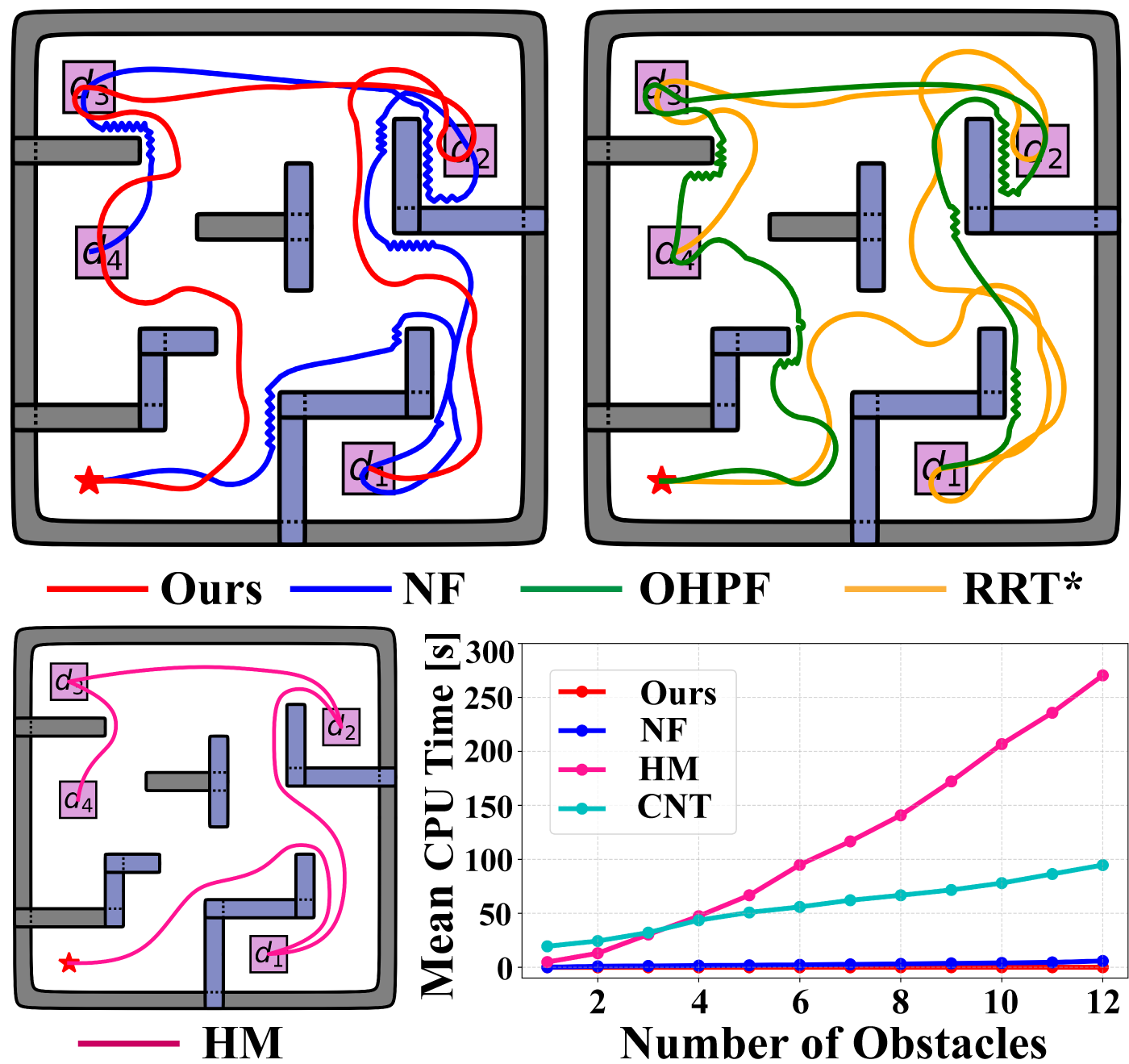
Figure 12: Top and Bottom Left: Comparison of the final trajectories via the proposed method (in red), NF without plan adaptation (in blue), OHPF without the search trees (in green), RRT^⋆ without plan adaptation (in orange), and HM without plan adaptation (in pink). The obstacles in grey are initially known and in blue are detected online. Bottom Right: Comparison of computation time between our incremental method (in red), and the baselines.

At time $t=0$, the robot starts from the initial position $(2.8m,0.4m)$ and orientation $\pi$. The task automaton $\mathcal{A}_{\varphi}$ is constructed with $29$ states and $474$ edges. The FTS associated with the regions of interest is initialized as a fully-connected graph that each edge is built as a HT consisting of an average of $9$ intermediate waypoints, with an average computation time of $0.103s$. The weight of each edge is estimated using the cost function in Sec. 4.1.1. Then, the product automaton $\widehat{\mathcal{A}}$ is constructed with $192$ states and $1435$ edges, of which the initial task plan is $P_{0}=p_{1}\,d_{1}\,d_{3}\,d_{2}$. Guided by this high-level plan, the robot navigates first towards task $p_{1}$ along the intermediate waypoints. Between any pair of the waypoint $(\nu_{n},\,\nu_{n+1})$, the initial navigation function $\varphi_{\texttt{NF}}$(q) is constructed using the associated transformations in (9). The mean computation time for $\varphi_{\texttt{NF}}(q)$ at every point within the workspace is $9.17ms$ and the corresponding potentials are visualized in Fig. 3 and 11. Given this navigation function, the oriented harmonic fields $\Upsilon(q)$ is constructed, with the associated orientation $\theta_{n+1}$, then the nonlinear controller in (24) is utilized to drive the robot towards the current goal as illustrated in Fig. 11. As the robot executes its current plan and explores the workspace gradually, new obstacles are discovered at discrete time instants, as shown in Fig. 11. For example, at $t=6.3s$ and $18.8s$, new obstacles are detected and block the way; the underlying navigation functions are updated incrementally by the approach described in Sec. 4.2.1. In detail, at $t=6.3s$, the estimated costs for the plans $p_{1}d_{1}d_{2}d_{3}$ and $p_{2}d_{1}d_{2}d_{3}$ are $17.1$ and $15.9$, respectively. Thus, the robot moves toward $p_{2}$ instead of $p_{1}$ due to the higher cost associated with rotation. The mean computation time for the new navigation functions are $13.94ms$ and $16.63ms$, respectively. The weight $\mathbf{w}$ in the control cost is updated by the strategy in Sec. 4.2.3 with the traversed edges in HT. Afterwards, the navigation map $\mathcal{G}$ is updated accordingly to satisfy the feasibility and cost minimization. The new task plan is $p_{2}d_{1}d_{3}d_{2}$. Given this new plan, the robot continues to navigate along the associated potential fields. At $t=61.7s$, the urgent task in region $u_{1}$ is triggered, thus the new subtask is added and the associated product automaton is reconstructed to get the new task plan $u_{1}d_{2}d_{3}$, as shown in Fig. 11. Finally, the whole task is accomplished in $122.5s$ and the resulting trajectory has a total distance $30.86m$.

5.3 Comparisons

To further demonstrate the effectiveness of our proposed Harmonic Tree (HT) structure, a quantitative comparison is conducted against five baselines: (i) the Navigation Function (NF) from Rimon (1990); Loizou (2017) without the high-level task adaptation; (ii) the oriented harmonic potential fields (OHPF) proposed in this work with the high-level task adaptation, but omitting the second-layer search trees; (iii) the Non-holonomic RRT^⋆ in LaValle (2006); Park & Kuipers (2015) without the high-level task adaptation; (iv) the harmonic maps (HM) in Vlantis et al. (2018) via the open-sourced implementation; and (v) the conformal navigation transformation (CNT) from Fan et al. (2022), which has to be modified considerably for the complex workspace here. As summarized in Table 1, the metrics to compare are computation time for each plan synthesis and adaptation, the total cost of final trajectory as the distance travelled, and whether oscillations appear during execution.

For easier comparison, a smaller workspace of size $4m\times 4m$ with $11$ overlapping obstacles is considered as shown in Fig. 12. The robot starts from $(0.5m,0.4m)$ with a prior knowledge of $3$ obstacles. The task requires the robot to surveil the regions of interest $d_{1},d_{2},d_{3},d_{4}$ in an arbitrary order. Other parameters are same to Sec. 5.1. The final trajectories and numerical results are shown in Fig. 12 and Table 1. The proposed HT exhibits lower cost for task completion with a fast planning and adaptation, with no collision or oscillations during execution. As for NF, a blind execution of the initial plan leads to a more costly trajectory with numerous oscillations since the gradients near the obstalce can not be tracked perfectly. Besides, the nominal NF can not control the final orientation as the robot approaches the task areas, resulting in high steering cost when task regions switch. In contrast, OHPF optimizes the orientations at each task region and adapts the high-level plan online as the proposed HT, leading to a much smaller execution time and overall cost. However, it is worth noting that without the guidance of search trees, oscillations can still occur close to obstacles for OHPF. Further, RRT^⋆ takes significantly more time to synthesize the initial plan and adapt the new plan, due to high computationally complexity of collision detection between samples. Namely, it takes around $83s$ to compute the complete plan for RRT^⋆, compared with merely $3.3s$ by the proposed HT. The HM method takes the shortest distance of $14.32m$ to finish the task with a longer planning time $12s$ due to the off-line construction of the navigation map with $2048$ boundary points. Similarly, the CNT method takes significantly more planning time and execution time (close to $26s$ and $87s$).

Lastly, the computational efficiency of the proposed iterative approach is compared with nominal NF, HM, and CNT, as summarized in Fig. 12. As the number of obstacles increases, the computation time of our method remains relatively low due to its analytical computation, incremental update and the hierarchical structure. In contrast, the nominal NF method requires nearly twice the time due to the frequent re-calculation of the potentials from scratch. Furthermore, the computation time for HM and CNT increases drastically with the number of boundary points (each obstacle has $2000$ boundary points), e.g., it takes more than $300s$ for HM with more than $12$ obstacles.

5.4 Hardware Experiments

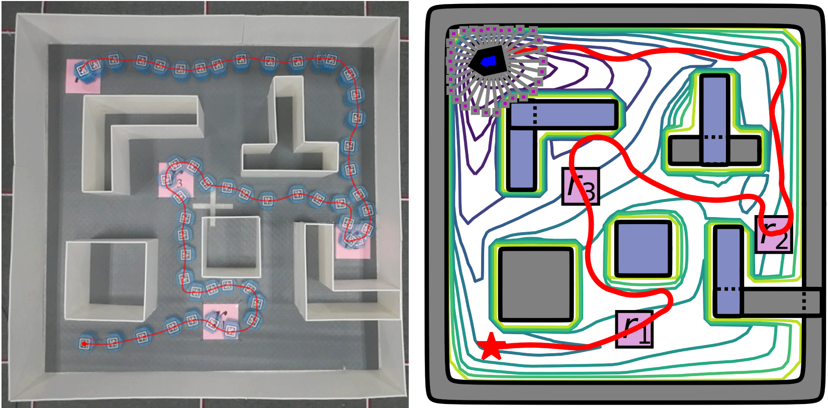
Figure 13: Left: Snapshots of hardware experiments. Right: Final trajectory with the final potential fields, where obstacles in blue are detected online.

The proposed method is deployed to a differential-driven robot of radius $r_{\texttt{r}}=0.1m$ As shown in Fig. 13, the workspace is constructed by whiteboards of size $2m\times 2m$, which has $2$ independent and $6$ overlapping obstacles. The controller gains in (24) are set to $k_{\upsilon}=0.15$ and $k_{\omega}=0.3$. The robot state is monitored by an overhead camera and the communication between the robot and the workstation is achieved by ROS with a frequency of $10$Hz. The point clouds are collected within a radius of $0.3$m around the robot. Other parameters are similar to the simulation study. The surveillance task is similar to the simulated case for regions $r_{1},r_{2},r_{3},r_{4}$. The robot starts from $(0.25m,0.2m)$ with orientation $0$. The initial task plan is derived within $0.48s$ as $r_{1}\,r_{2}\,r_{3}\,r_{4}$. During the online execution, the robot adjusts its high-level plan and underlying harmonic potentials as the environment changes. As the robot detects more obstacles and familiar with the workspace, the task plan is updated as $r_{1}r_{3}r_{4}r_{2}$ and finally converges to $r_{1}r_{3}r_{2}r_{4}$. The whole task is accomplished in $169s$. The resulting trajectory is shown in Fig. 13 with a total distance $5.83m$, which is safe and smooth despite of the localization and control uncertainties. These results are consistent with the simulations above.

6 Conclusion

This work proposes an automated framework for task and motion planning, employing harmonic potentials for navigation and oriented search trees for planning. The design and construction of the search tree is specifically customized for the task automaton and co-designed with the underlying navigation controllers based on harmonic potentials. Efficient and secure task execution is ensured for partially-known workspace. Future work involves the consideration of dynamic environments, multi-agent scenarios and 3D navigation.

References

- Baier & Katoen (2008) Baier, C., & Katoen, J.-P. (2008). Principles of model checking. MIT press.
- Fainekos et al. (2009) Fainekos, G. E., Girard, A., Kress-Gazit, H., & Pappas, G. J. (2009). Temporal logic motion planning for dynamic robots. Automatica, 45, 343–352.
- Fan et al. (2022) Fan, L., Liu, J., Zhang, W., & Xu, P. (2022). Robot navigation in complex workspaces using conformal navigation transformations. IEEE Robotics and Automation Letters, 8, 192–199.
- Filippidis & Kyriakopoulos (2011) Filippidis, I., & Kyriakopoulos, K. J. (2011). Adjustable navigation functions for unknown sphere worlds. In IEEE Conference on Decision and Control and European Control Conference (pp. 4276–4281). IEEE.
- Garrett et al. (2021) Garrett, C. R., Chitnis, R., Holladay, R., Kim, B., Silver, T., Kaelbling, L. P., & Lozano-Pérez, T. (2021). Integrated task and motion planning. Annual review of control, robotics, and autonomous systems, 4, 265–293.
- Gavin (2019) Gavin, H. P. (2019). The levenberg-marquardt algorithm for nonlinear least squares curve-fitting problems. Department of civil and environmental engineering, Duke University, 19.
- Ghallab et al. (2004) Ghallab, M., Nau, D., & Traverso, P. (2004). Automated Planning: theory and practice. Elsevier.
- Guo et al. (2018) Guo, M., Andersson, S., & Dimarogonas, D. V. (2018). Human-in-the-loop mixed-initiative control under temporal tasks. In IEEE International Conference on Robotics and Automation (ICRA) (pp. 6395–6400).
- Guo & Dimarogonas (2015) Guo, M., & Dimarogonas, D. V. (2015). Multi-agent plan reconfiguration under local ltl specifications. The International Journal of Robotics Research, 34, 218–235.
- Hsu et al. (2006) Hsu, D., Latombe, J.-C., & Kurniawati, H. (2006). On the probabilistic foundations of probabilistic roadmap planning. The International Journal of Robotics Research, 25, 627–643.
- Janson et al. (2015) Janson, L., Schmerling, E., Clark, A., & Pavone, M. (2015). Fast marching tree: A fast marching sampling-based method for optimal motion planning in many dimensions. The International Journal of Robotics Research, 34, 883–921.
- Karaman & Frazzoli (2011) Karaman, S., & Frazzoli, E. (2011). Sampling-based algorithms for optimal motion planning. The International Journal of Robotics Research, 30, 846–894.
- Khalil (2002) Khalil, H. (2002). Nonlinear systems; 3rd ed.. Upper Saddle River, NJ: Prentice Hall.
- Khatib (1986) Khatib, O. (1986). Real-time obstacle avoidance for manipulators and mobile robots. In Autonomous robot vehicles (pp. 396–404). Springer.
- Khatib (1999) Khatib, O. (1999). Mobile manipulation: The robotic assistant. Robotics and Autonomous Systems, 26, 175–183.
- Kim et al. (2022) Kim, B., Shimanuki, L., Kaelbling, L. P., & Lozano-Pérez, T. (2022). Representation, learning, and planning algorithms for geometric task and motion planning. The International Journal of Robotics Research, 41, 210–231.
- Kim & Khosla (1992) Kim, J.-o., & Khosla, P. (1992). Real-time obstacle avoidance using harmonic potential functions. IEEE Transactions on Robotics and Automation, 8, 338–349.
- Ko et al. (2013) Ko, I., Kim, B., & Park, F. C. (2013). Vf-rrt: Introducing optimization into randomized motion planning. In IEEE Asian Control Conference (ASCC) (pp. 1–5).
- Koditschek (1987) Koditschek, D. (1987). Exact robot navigation by means of potential functions: Some topological considerations. In IEEE International Conference on Robotics and Automation (pp. 1–6). volume 4.
- LaValle (2006) LaValle, S. M. (2006). Planning algorithms. Cambridge university press.
- Leahy et al. (2021) Leahy, K., Serlin, Z., Vasile, C.-I., Schoer, A., Jones, A. M., Tron, R., & Belta, C. (2021). Scalable and robust algorithms for task-based coordination from high-level specifications (scratches). IEEE Transactions on Robotics, 38, 2516–2535.
- Li & Tanner (2018) Li, C., & Tanner, H. G. (2018). Navigation functions with time-varying destination manifolds in star worlds. IEEE Transactions on Robotics, 35, 35–48.
- Lindemann et al. (2021) Lindemann, L., Matni, N., & Pappas, G. J. (2021). Stl robustness risk over discrete-time stochastic processes. In IEEE Conference on Decision and Control (CDC) (pp. 1329–1335).
- Loizou (2011) Loizou, S. G. (2011). Closed form navigation functions based on harmonic potentials. In IEEE Conference on Decision and Control and European Control Conference (pp. 6361–6366).
- Loizou (2017) Loizou, S. G. (2017). The navigation transformation. IEEE Transactions on Robotics, 33, 1516–1523.
- Loizou & Rimon (2021) Loizou, S. G., & Rimon, E. D. (2021). Correct-by-construction navigation functions with application to sensor based robot navigation. arXiv preprint arXiv:2103.04445, .
- Loizou & Rimon (2022) Loizou, S. G., & Rimon, E. D. (2022). Mobile robot navigation functions tuned by sensor readings in partially known environments. IEEE Robotics and Automation Letters, 7, 3803–3810.
- Luo et al. (2021) Luo, X., Kantaros, Y., & Zavlanos, M. M. (2021). An abstraction-free method for multirobot temporal logic optimal control synthesis. IEEE Transactions on Robotics, 37, 1487–1507.
- Ogren & Leonard (2005) Ogren, P., & Leonard, N. E. (2005). A convergent dynamic window approach to obstacle avoidance. IEEE Transactions on Robotics, 21, 188–195.
- Otte & Frazzoli (2016) Otte, M., & Frazzoli, E. (2016). Rrtx: Asymptotically optimal single-query sampling-based motion planning with quick replanning. The International Journal of Robotics Research, 35, 797–822.
- Panagou (2014) Panagou, D. (2014). Motion planning and collision avoidance using navigation vector fields. In IEEE International Conference on Robotics and Automation (ICRA) (pp. 2513–2518).
- Park & Kuipers (2015) Park, J. J., & Kuipers, B. (2015). Feedback motion planning via non-holonomic rrt for mobile robots. In IEEE/RSJ International Conference on Intelligent Robots and Systems (IROS) (pp. 4035–4040).
- Qureshi & Ayaz (2016) Qureshi, A. H., & Ayaz, Y. (2016). Potential functions based sampling heuristic for optimal path planning. Autonomous Robots, 40, 1079–1093.
- Rimon (1990) Rimon, E. (1990). Exact robot navigation using artificial potential functions. Ph.D. thesis Yale University.
- Rousseas et al. (2021) Rousseas, P., Bechlioulis, C., & Kyriakopoulos, K. J. (2021). Harmonic-based optimal motion planning in constrained workspaces using reinforcement learning. IEEE Robotics and Automation Letters, 6, 2005–2011.
- Rousseas et al. (2022a) Rousseas, P., Bechlioulis, C. P., & Kyriakopoulos, K. J. (2022a). Optimal motion planning in unknown workspaces using integral reinforcement learning. IEEE Robotics and Automation Letters, 7, 6926–6933.
- Rousseas et al. (2022b) Rousseas, P., Bechlioulis, C. P., & Kyriakopoulos, K. J. (2022b). Trajectory planning in unknown 2d workspaces: A smooth, reactive, harmonics-based approach. IEEE Robotics and Automation Letters, 7, 1992–1999.
- Shen et al. (2021) Shen, Z., Wilson, J., Harvey, R., & Gupta, S. (2021). Smarrt: Self-repairing motion-reactive anytime rrt for dynamic environments. arXiv preprint arXiv:2109.05043, .
- Tahir et al. (2018) Tahir, Z., Qureshi, A. H., Ayaz, Y., & Nawaz, R. (2018). Potentially guided bidirectionalized rrt* for fast optimal path planning in cluttered environments. Robotics and Autonomous Systems, 108, 13–27.
- Valbuena & Tanner (2012) Valbuena, L., & Tanner, H. G. (2012). Hybrid potential field based control of differential drive mobile robots. Journal of Intelligent & Robotic systems, 68, 307–322.
- Vasilopoulos et al. (2022) Vasilopoulos, V., Pavlakos, G., Schmeckpeper, K., Daniilidis, K., & Koditschek, D. E. (2022). Reactive navigation in partially familiar planar environments using semantic perceptual feedback. The International Journal of Robotics Research, 41, 85–126.
- Vlantis et al. (2018) Vlantis, P., Vrohidis, C., Bechlioulis, C. P., & Kyriakopoulos, K. J. (2018). Robot navigation in complex workspaces using harmonic maps. In 2018 IEEE International Conference on Robotics and Automation (ICRA) (pp. 1726–1731). IEEE.
- Wang (2023) Wang, S. (2023). Harmonic tree. https://shuaikang-wang.github.io/HarmonicTree/.
- Warren (1989) Warren, C. W. (1989). Global path planning using artificial potential fields. In IEEE International Conference on Robotics and Automation (ICRA) (pp. 316–317).