Importance Sparsification for Sinkhorn Algorithm

Abstract

Sinkhorn algorithm has been used pervasively to approximate the solution to optimal transport (OT) and unbalanced optimal transport (UOT) problems. However, its practical application is limited due to the high computational complexity. To alleviate the computational burden, we propose a novel importance sparsification method, called Spar-Sink, to efficiently approximate entropy-regularized OT and UOT solutions. Specifically, our method employs natural upper bounds for unknown optimal transport plans to establish effective sampling probabilities, and constructs a sparse kernel matrix to accelerate Sinkhorn iterations, reducing the computational cost of each iteration from $O(n^{2})$ to $\widetilde{O}(n)$ for a sample of size $n$. Theoretically, we show the proposed estimators for the regularized OT and UOT problems are consistent under mild regularity conditions. Experiments on various synthetic data demonstrate Spar-Sink outperforms mainstream competitors in terms of both estimation error and speed. A real-world echocardiogram data analysis shows Spar-Sink can effectively estimate and visualize cardiac cycles, from which one can identify heart failure and arrhythmia. To evaluate the numerical accuracy of cardiac cycle prediction, we consider the task of predicting the end-systole time point using the end-diastole one. Results show Spar-Sink performs as well as the classical Sinkhorn algorithm, requiring significantly less computational time.

Keywords: echocardiogram analysis, element-wise sampling, importance sampling, (unbalanced) optimal transport, Wasserstein-Fisher-Rao distance

1 Introduction

The optimal transport (OT) problem, initiated by Gaspard Monge in the 18th century, aims to calculate the Wasserstein distance that quantifies the discrepancy between two probability measures. Recently, the Wasserstein distance has played an increasingly preponderant role in machine learning (Courty et al., 2016; Arjovsky et al., 2017; Meng et al., 2019; Muzellec et al., 2020; Balaji et al., 2020), statistics (Flamary et al., 2018; Panaretos and Zemel, 2019; Meng et al., 2020; Dubey and Müller, 2020), computer vision (Ferradans et al., 2014; Su et al., 2015; Solomon et al., 2015; Xu et al., 2019), biomedical research (Tanay and Regev, 2017; Schiebinger et al., 2019; Marouf et al., 2020), among others. We refer to Peyré and Cuturi (2019) and Panaretos and Zemel (2019) for recent reviews.

Despite the broad range of applications, existing methods for computing the Wasserstein distance suffer from a huge computational burden when the sample size $n$ is large. Specifically, traditional approaches involve solving differential equations (Brenier, 1997; Benamou et al., 2002) or linear programming problems (Rubner et al., 1997; Pele and Werman, 2009). The computational cost of such methods is of the order $O(n^{3}\log(n))$.

To alleviate the computational burden, a large number of efficient computational tools have been developed in the recent decade. One major class of approaches is called the regularization-based method, which solves an entropy-regularized OT problem instead of the original one (Cuturi, 2013). The regularized OT problem is unconstrained and convex with a differentiable objective function, and can be solved using the Sinkhorn algorithm (Sinkhorn and Knopp, 1967) in $O(Ln^{2})$ time, where $L$ is the number of iterations. It has been shown that regularized OT solutions possess better theoretical properties than the unregularized counterparts (Montavon et al., 2016; Rigollet and Weed, 2018; Feydy et al., 2019; Peyré and Cuturi, 2019). Another advantage of the regularization-based approach is that it can be applied to a generic class of unbalanced optimal transport (UOT) problems (Chizat et al., 2018b). The UOT problem relaxes the strict marginal constraints of OT by allowing partial displacement of mass, making it more suitable for applications that involve both mass variation (e.g., creation or destruction) and mass transportation (Frogner et al., 2015; Chizat et al., 2018b; Zhou et al., 2018; Wang et al., 2020). The Sinkhorn algorithm can be naturally extended to approximate UOT solutions, also requiring an $O(Ln^{2})$ computational cost (Chizat et al., 2018b; Pham et al., 2020). In general, the Sinkhorn algorithm enables researchers to approximate the OT and UOT solutions efficiently, and thus has been extensively studied in the recent decade (Cuturi and Doucet, 2014; Genevay et al., 2019; Feydy et al., 2019; Lin et al., 2019b; Pham et al., 2020). There also exist slicing-based methods to approximate the Wasserstein distance (Pitié et al., 2005; Rabin et al., 2011; Bonneel et al., 2015; Meng et al., 2019; Deshpande et al., 2019; Zhang et al., 2021a; Nguyen et al., 2021, 2023), and such methods are beyond the scope of this paper. A recent review of such methods can be found in Nadjahi (2021).

Despite the wide application, the time and memory requirements of the Sinkhorn algorithm grow quadratically with $n$, which hinders its broad applicability to many large-scale optimal transport problems. To address the computational bottleneck, many efficient variants of the Sinkhorn algorithm have been proposed in recent years (Solomon et al., 2015; Altschuler et al., 2019; Pham et al., 2020; Scetbon and Cuturi, 2020; Scetbon et al., 2021; Klicpera et al., 2021; Le et al., 2021; Séjourné et al., 2022; Liao et al., 2022a, b). For example, in contrast to the scheme of Sinkhorn that updates all rows and columns of the transport plan at each step, the variants including greedy Sinkhorn (Greenkhorn) (Altschuler et al., 2017; Lin et al., 2022), randomized Sinkhorn (Randkhorn) (Lin et al., 2019a), and screening Sinkhorn (Screenkhorn) (Alaya et al., 2019) only update partial row(s) or column(s) in each iteration, based on different selection criteria. These variants have been shown to converge faster in practice, making them appealing for large-scale applications. In addition, Xie et al. (2020) developed an inexact proximal point method to address numerical instability issues of Sinkhorn algorithm.

Nevertheless, most of the existing variants of the Sinkhorn algorithm still require an $O(Ln^{2})$ computational cost. One exception is the Nys-Sink approach proposed by Altschuler et al. (2019), where the authors proposed to accelerate the Sinkhorn algorithm using the Nyström method, a well-known technique for low-rank matrix approximation (Kumar et al., 2012). The computational complexity of Nys-Sink is reduced to $O(Lrn)$, where $r\leq n$ denotes the estimated rank of the kernel matrix $\mathbf{K}$ with respect to (w.r.t.) the Sinkhorn algorithm. Further details of the kernel matrix $\mathbf{K}$ will be provided in the subsequent section. However, the Nys-Sink method suffers from two limitations: it requires (i) $\mathbf{K}$ to be symmetric positive semi-definite, and (ii) $\mathbf{K}$ possessing a low-rank structure. Such constraints restrict the applicability of Nys-Sink in many practical scenarios. For instance, the Wasserstein-Fisher-Rao distance (Kondratyev et al., 2016; Chizat et al., 2018a; Liero et al., 2018), a popular distance in UOT problems, is associated with a kernel matrix $\mathbf{K}$ that is highly sparse and nearly full-rank; see Section 2 for more details. The Nys-Sink method thus may be ineffective for estimating the Wasserstein-Fisher-Rao distance in large-scale UOT problems. Therefore, the development of an efficient variant of the Sinkhorn algorithm capable of handling large-scale asymmetric and nearly full-rank kernel matrix $\mathbf{K}$ remains a blank field requiring further research.

In this paper, we propose a randomized sparsification variant of the Sinkhorn algorithm, called Spar-Sink, for both OT and UOT problems. Specifically, we construct a sparsified kernel matrix $\widetilde{\mathbf{K}}$ by carefully sampling $s=o(n^{2})$ elements from $\mathbf{K}$ and setting the remaining ones to zero. We then leverage $\widetilde{\mathbf{K}}$ and sparse matrix multiplications to accelerate the iterations in the Sinkhorn algorithm, reducing the computational cost from $O(n^{2})$ to $O(s)$ per iteration.

The key to the success of the proposed strategy is developing an effective sampling probability. We demonstrate that both OT and UOT problems provide natural upper bounds for the elements in the unknown optimal transport plan. Drawing inspiration from the importance sampling technique, we employ such upper bounds to construct sampling probabilities. Theoretically, we show that the proposed estimators for entropic OT and UOT problems are consistent when $s=\widetilde{O}(n)$ under certain regularity conditions, where $\widetilde{O}(\cdot)$ suppresses logarithmic factors. Extensive simulations show Spar-Sink yields much smaller estimation errors compared with mainstream competitors.

We consider a real-world echocardiogram data analysis to demonstrate the performance of Spar-Sink. Specifically, we propose using the Wasserstein-Fisher-Rao (WFR) distance (Kondratyev et al., 2016; Chizat et al., 2018a; Liero et al., 2018), a special metric in UOT problems, to characterize the similarity between any two frames in an echocardiogram video. Compared to the Wasserstein distance, the WFR distance prevents long-range mass transportation between two distributions, and thus can achieve a balance between global transportation and local truncation. Intuitively, such a distance is more consistent with the nature of myocardial motion that the cardiac muscle would not transport too far. We focus on the task of cardiac cycle identification, which is an essential but laborious task for the downstream assessment of cardiac function (Ouyang et al., 2020). We apply the proposed Spar-Sink algorithm to approximate the WFR distance and predict cardiac cycles automatically and efficiently, which has the potential to obviate the heavy work for cardiologists. Empirical results show that our method can effectively estimate and visualize cardiac cycles, with the potential to identify heart failure and arrhythmia from the results. To evaluate the numerical accuracy of cardiac cycle prediction, we predict the end-systole time point using the end-diastole one. The results show Spar-Sink achieves the same prediction accuracy as the Sinkhorn algorithm while requiring much less computational time.

A problem closely related to the optimal transport is the (fixed-support) Wasserstein barycenter problem, which aims to calculate the barycenter of a set of probability measures (whose supports are predetermined) in the Wasserstein space (Agueh and Carlier, 2011). Extending the work of Cuturi (2013), Wasserstein barycenters can also be approximated by entropic smoothing (Cuturi and Doucet, 2014) using the iterative Bregman projection (IBP) algorithm (Benamou et al., 2015). Concerning the computational hardness, significant research has been devoted to further enhancing the celebrated IBP algorithm (Cuturi and Peyré, 2018; Kroshnin et al., 2019; Lin et al., 2020; Guminov et al., 2021). In this paper, we also extend the idea of sparsification to the IBP algorithm, efficiently approximating Wasserstein barycenters.

The remainder of this paper is organized as follows. We start in Section 2 by introducing the background of OT and UOT problems. In Section 3, we develop the sampling probabilities and provide the details of the main algorithm. The theoretical properties of the proposed estimators are presented in Section 4. We examine the performance of the proposed method through extensive synthetic data sets in Section 5. Echocardiogram data analysis is provided in Section 6. Extensions, technical details, and additional numerical results and applications are relegated to the Appendix.

2 Background

Here we summarize the notation used throughout the paper. We adopt the standard convention of using uppercase boldface letters for matrices, lowercase boldface letters for vectors, and regular font for scalars. We denote non-negative real numbers by $\mathbb{R}_{+}$, the set of integers $\{1,\ldots,n\}$ by $[n]$, and the $(n-1)$-dimensional simplex by $\Delta^{n-1}=\{\bm{x}\in\mathbb{R}_{+}^{n}:\sum_{i=1}^{n}x_{i}=1\}$. An empirical measure $\mu$ supported by $n$ points $\bm{x}_{i}\in\mathbb{R}^{d},i\in[n]$ is defined as $\mu=\sum_{i=1}^{n}a_{i}\delta_{\bm{x}_{i}}$, where $\delta_{\cdot}$ is the Dirac delta function and $\bm{a}=(a_{1},\ldots,a_{n})$ is the corresponding histogram in $\mathbb{R}_{+}^{n}$. For two histograms $\bm{a},\bm{b}\in\mathbb{R}_{+}^{n}$, we define the Kullback-Leibler divergence $\mathrm{KL}(\bm{a}\|\bm{b})$ between $\bm{a}$ and $\bm{b}$ by $\mathrm{KL}(\bm{a}\|\bm{b})=\sum_{i=1}^{n}a_{i}\log(a_{i}/b_{i})-a_{i}+b_{i}$, where we adopt the standard convention that $0\log(0)=0$. For a coupling matrix $\mathbf{T}\in\mathbb{R}_{+}^{n\times n}$, its Shannon entropy is defined as $H(\mathbf{T})=-\sum_{i,j}T_{ij}(\log(T_{ij})-1)$. We use $\|\mathbf{A}\|_{2}$ to denote the spectral norm (i.e., maximal singular value) of a matrix $\mathbf{A}$, and its condition number is defined as $\|\mathbf{A}\|_{2}/\lambda_{\min}(\mathbf{A})$, where $\lambda_{\min}(\cdot)$ is the minimal singular value. For $\mathbf{A}$ and $\mathbf{B}$ of the same dimension, we denote their Frobenius inner product by $\langle\mathbf{A},\mathbf{B}\rangle=\sum_{i,j}A_{ij}B_{ij}$. For a vector $\bm{x}$, we use $\|\bm{x}\|_{p}$ and $\|\bm{x}\|_{\infty}$ to represent its $\ell_{p}$ norm and infinity norm, respectively. For two non-negative sequences $(x_{n})_{n}$ and $(y_{n})_{n}$, we denote $x_{n}=\widetilde{O}(y_{n})$ if there exist constants $c,c^{\prime}>0$ such that $x_{n}\leq c^{\prime}y_{n}(\log(n))^{c}$.

2.1 Optimal Transport Problem and Sinkhorn Algorithm

To begin with, we consider two empirical probability measures $\bm{a}\in\Delta^{m-1}$ and $\bm{b}\in\Delta^{n-1}$. For brevity, we focus on the case of $m=n$ in this paper, since the extension to unequal cases is straightforward. The goal of the optimal transport problem is to compute the minimal effort of moving the masses $\bm{a}$ and $\bm{b}$ onto each other, according to some ground cost between the supports. Due to Kantorovich (1942), the modern OT formulation takes the form

$$\operatorname{OT}(\bm{a},\bm{b}):=\min_{\mathbf{T}\in\mathcal{U}(\bm{a},\bm{b})}\langle\mathbf{T},\mathbf{C}\rangle,$$ (1)

where $\mathcal{U}(\bm{a},\bm{b}):=\{\mathbf{T}\in\mathbb{R}_{+}^{n\times n}:\mathbf{T}\mathbf{1}_{n}=\bm{a},\mathbf{T}^{\top}\mathbf{1}_{n}=\bm{b}\}$ is the set of admissible transportation plans, i.e., all joint probability distributions with marginals $\bm{a},\bm{b}$, and $\mathbf{C}\in\mathbb{R}_{+}^{n\times n}$ is a given cost matrix with bounded entries. The solutions to (1) are called the optimal transport plan. When $\mathbf{C}$ is a pairwise distance matrix of the power $p$, $W_{p}(\cdot,\cdot):=\operatorname{OT}(\cdot,\cdot)^{1/p}$ defines the $p$-Wasserstein distance on $\Delta^{n-1}$.

A clear drawback of OT is that the computational cost of directly solving the problem (1) is hugely prohibitive. Indeed, conventional methods require $O(n^{3}\log(n))$ time (Brenier, 1997; Rubner et al., 1997; Benamou et al., 2002; Pele and Werman, 2009). Even the fastest algorithms known to date for (1) have a computational complexity of at least $O(n^{2.5}\log(n))$ (Lee and Sidford, 2014, 2015; Guo et al., 2020; An et al., 2022).

To approximate the solution to the OT problem efficiently, Cuturi (2013) introduced an entropic penalty term to (1) and turned it into an entropy-regularized OT problem

$$\operatorname{OT}_{\varepsilon}(\bm{a},\bm{b}):=\min_{\mathbf{T}\in\mathcal{U}(\bm{a},\bm{b})}\langle\mathbf{T},\mathbf{C}\rangle-\varepsilon H(\mathbf{T}),$$ (2)

where the regularization parameter $\varepsilon>0$ controls the strength of the penalty term. Let $\mathbf{T}_{\varepsilon}^{\ast}\in\mathbb{R}^{n\times n}$ be the solution to (2). It is known that when $\varepsilon\to 0$, $\operatorname{OT}_{\varepsilon}(\bm{a},\bm{b})\to\operatorname{OT}(\bm{a},\bm{b})$; when $\varepsilon\to\infty$, $\mathbf{T}_{\varepsilon}^{\ast}\to\bm{a}\bm{b}^{\top}$ (Peyré and Cuturi, 2019).

In general, the solution $\mathbf{T}_{\varepsilon}^{\ast}$ is a projection onto $\mathcal{U}(\bm{a},\bm{b})$ of the kernel matrix $\mathbf{K}:=\exp(-\mathbf{C}/\varepsilon)$. The $(i,j)$th entry of $\mathbf{K}$ is given by $K_{ij}=\exp(-C_{ij}/\varepsilon)$. Indeed, for two (unknown) convergent scaling vectors $\bm{u}^{\ast},\bm{v}^{\ast}\in\mathbb{R}_{+}^{n}$, the unique solution $\mathbf{T}_{\varepsilon}^{\ast}$ takes the form

$$\mathbf{T}_{\varepsilon}^{\ast}=\operatorname{diag}(\bm{u}^{\ast})\mathbf{K}\operatorname{diag}(\bm{v}^{\ast}).$$ (3)

Based on the equation (3), $\mathbf{T}_{\varepsilon}^{\ast}$ can be approximated by the celebrated Sinkhorn algorithm using iterative matrix scaling (Sinkhorn and Knopp, 1967; Cuturi, 2013), requiring a computational cost of the order $O(Ln^{2})$. The pseudocode for the Sinkhorn algorithm is shown in Algorithm 1, where the operator $\oslash$ denotes the element-wise division.

Algorithm 1 SinkhornOT($\mathbf{K},\bm{a},\bm{b},\delta$)

1:Initialize: $t\leftarrow 0;\bm{v}^{(0)}\leftarrow\mathbf{1}_{n}$

2:repeat

3:     $t\leftarrow t+1$

4:     $\bm{u}^{(t)}\leftarrow\bm{a}\oslash\mathbf{K}\bm{v}^{(t-1)};\quad\bm{v}^{(t)}\leftarrow\bm{b}\oslash\mathbf{K}^{\top}\bm{u}^{(t)}$

5:until $\|\bm{u}^{(t)}-\bm{u}^{(t-1)}\|_{1}+\|\bm{v}^{(t)}-\bm{v}^{(t-1)}\|_{1}\leq\delta$

6:Output: $\mathbf{T}_{\varepsilon}^{\ast}=\operatorname{diag}(\bm{u}^{(t)})\mathbf{K}\operatorname{diag}(\bm{v}^{(t)})$

2.2 Unbalanced Optimal Transport Problem

When $\bm{a},\bm{b}\in\mathbb{R}_{+}^{n}$ are two arbitrary positive measures such that their total mass does not equal each other, the marginal constraints in the classical OT problem (1) are no longer valid. To overcome such an obstacle, researchers extended the classical optimal transport problem to the so-called unbalanced optimal transport (UOT) problem by relaxing the marginal constraints. In the literature, there exist several different formulations of the UOT problem; see Liero et al. (2016) and Chizat et al. (2018c) for reference. In this paper, we focus on the static formulation that only involves a minor modification of the initial linear program of OT. Specifically, the UOT problem between $\bm{a}$ and $\bm{b}$ is defined as

$$\operatorname{UOT}(\bm{a},\bm{b}):=\min_{\mathbf{T}\in\mathbb{R}_{+}^{n\times n}}\langle\mathbf{T},\mathbf{C}\rangle+\lambda\mathrm{KL}(\mathbf{T}\mathbf{1}_{n}\|\bm{a})+\lambda\mathrm{KL}(\mathbf{T}^{\top}\mathbf{1}_{n}\|\bm{b}).$$ (4)

Here, $\lambda>0$ is a regularization parameter that balances the trade-off between the transportation effort and maintaining the global structure of input measures. Intuitively, mass transportation increases with larger $\lambda$. Note that when $\|\bm{a}\|_{1}=\|\bm{b}\|_{1}$ and $\lambda\rightarrow\infty$, the UOT problem (4) degenerates to the classical OT problem (1).

One particular solution to the UOT problem is the so-called Wasserstein-Fisher-Rao distance (Kondratyev et al., 2016; Chizat et al., 2018a; Liero et al., 2018). Such a distance is associated with a cost matrix $\mathbf{C}=(C_{ij})$ such that $C_{ij}=-\log\left[\cos_{+}^{2}\left(d_{ij}/(2\eta)\right)\right]$, where $d_{ij}$ is a distance and $\cos_{+}:z\mapsto\cos\left(\min\left(z,\pi/2\right)\right)$. Here, the parameter $\eta$ controls the sparsity level in the kernel matrix $\mathbf{K}$, such that a smaller value of $\eta$ is associated with a sparser $\mathbf{K}$. More precisely, when $d_{ij}\geq\pi\eta$, it follows that $C_{ij}=\infty$ and thus $K_{ij}=0$, that is, the transportation between $a_{i}$ and $b_{j}$ is blocked. Hence, a smaller $\eta$ causes more elements in $\mathbf{K}$ to be truncated to zero, resulting in a sparser matrix. Moreover, a small $\eta$ leads to the diagonal or block-diagonal structure in $\mathbf{K}$, resulting in a large rank of the kernel matrix. The $\lambda$-Wasserstein-Fisher-Rao distance is defined as $\operatorname{WFR}_{\lambda}(\cdot,\cdot):=\operatorname{UOT}(\cdot,\cdot)^{1/2}$. Such a distance has been widely applied in natural language processing (Wang et al., 2020), earthquake location problems (Zhou et al., 2018), shape modification, color transfer, and growth models (Chizat et al., 2018b).

Similar to the classical OT problem, the exact computation of the UOT problem is not scalable in terms of the number of support points $n$. Inspired by the success of entropy-regularized OT, we consider the entropic version of the UOT problem, defined as

$$\operatorname{UOT}_{\lambda,\varepsilon}(\bm{a},\bm{b}):=\min_{\mathbf{T}\in\mathbb{R}_{+}^{n\times n}}\langle\mathbf{T},\mathbf{C}\rangle+\lambda\mathrm{KL}(\mathbf{T}\mathbf{1}_{n}\|\bm{a})+\lambda\mathrm{KL}(\mathbf{T}^{\top}\mathbf{1}_{n}\|\bm{b})-\varepsilon H(\mathbf{T}),$$ (5)

with given parameters $\lambda,\varepsilon>0$. Similarly, we introduce the kernel matrix $\mathbf{K}=\exp(-\mathbf{C}/\varepsilon)$ and solve the problem (5) by iterative matrix scaling. Algorithm 2 proposed by Chizat et al. (2018b) is a straightforward generalization of the Sinkhorn algorithm from OT problems to UOT problems. The output of Algorithm 2 is the unique solution to the problem (5). Note that when $\lambda\rightarrow\infty$, we have $\lambda/(\lambda+\varepsilon)\to 1$ and thus Algorithm 2 degenerates to Algorithm 1.

Algorithm 2 SinkhornUOT($\mathbf{K},\bm{a},\bm{b},\lambda,\varepsilon,\delta$)

1:Initialize: $t\leftarrow 0;\bm{u}^{(0)},\bm{v}^{(0)}\leftarrow\mathbf{1}_{n}$

2:repeat

3:     $t\leftarrow t+1$

4:     $\bm{u}^{(t)}\leftarrow\left(\bm{a}\oslash\mathbf{K}\bm{v}^{(t-1)}\right)^{\lambda/(\lambda+\varepsilon)};\quad\bm{v}^{(t)}\leftarrow\left(\bm{b}\oslash\mathbf{K}^{\top}\bm{u}^{(t)}\right)^{\lambda/(\lambda+\varepsilon)}$

5:until $\|\bm{u}^{(t)}-\bm{u}^{(t-1)}\|_{1}+\|\bm{v}^{(t)}-\bm{v}^{(t-1)}\|_{1}\leq\delta$

6:Output: $\mathbf{T}_{\lambda,\varepsilon}^{\ast}=\operatorname{diag}(\bm{u}^{(t)})\mathbf{K}\operatorname{diag}(\bm{v}^{(t)})$

3 Main Algorithm

In this section, we present our main algorithm called importance sparsification for the Sinkhorn algorithm (Spar-Sink). The idea is first to apply element-wise subsampling on the kernel matrix $\mathbf{K}$ to obtain a sparse sketch $\widetilde{\mathbf{K}}$. We then use $\widetilde{\mathbf{K}}$ as a surrogate for $\mathbf{K}$ and use sparse matrix multiplication techniques to accelerate the iterations in the Sinkhorn algorithm.

3.1 Matrix Sparsification and Importance Sampling

Given an input matrix $\mathbf{A}$, element-wise matrix sparsification seeks to select (and rescale) a small set of elements from $\mathbf{A}$ and produce a sparse sketch $\widetilde{\mathbf{A}}$, that can serve as a good proxy for $\mathbf{A}$. Pioneered by Achlioptas and Mcsherry (2007), previous research has been dedicated to developing various sampling frameworks and probabilities to construct an effective $\widetilde{\mathbf{A}}$ (Arora et al., 2006; Candès and Tao, 2010; Drineas and Zouzias, 2011; Achlioptas et al., 2013; Chen et al., 2014; Gupta and Sidford, 2018). Finding such a matrix $\widetilde{\mathbf{A}}$ can not only be used to accelerate matrix operations (Drineas et al., 2006; Mahoney, 2011; Gupta and Sidford, 2018; Li et al., 2023), but also has broad applications in recovering data with missing features, and preserving privacy when the data cannot be fully observed (Kundu et al., 2017).

In this study, we implement the matrix sparsification via the Poisson sampling framework following the recent work of Braverman et al. (2021). Poisson sampling looks at each element and determines whether to include it in the subsample according to a specific probability independently. Compared to the other commonly used subsampling technique, sampling with replacement, Poisson sampling has a higher approximation accuracy in some situations and is more convenient to implement in distributed systems; see Wang and Zou (2021) for a comprehensive comparison.

The key to success is how to construct an effective $\widetilde{\mathbf{K}}$ that leads to an asymptotically unbiased solution with a relatively small variance. To achieve the goal, we develop sampling probabilities based on the idea behind importance sampling, which is widely used for variance-reduction in numerical integration (Liu, 1996, 2008). The importance sampling technique can be described as follows: to approximate the summation $\mu=\sum_{i=1}^{N}f_{i}$ with $f_{i}\geq 0$, we assign each $i\in[N]$ a probability $q_{i}\geq 0$ such that $\sum_{i=1}^{N}q_{i}=1$, and then sample a subset of size $s(<N)$, $\{i_{t}\}_{t=1}^{s}$, from $[N]$ based on the probabilities $\{q_{i}\}_{i=1}^{N}$. The summation then can be approximated by $\mu\approx\sum_{t=1}^{s}f_{i_{t}}/(sq_{i_{t}})$. Kahn and Marshall (1953) showed when $f_{i}$’s are known, the optimal sampling probability $q_{i}$ in terms of variance-reduction is proportional to $f_{i}$ (Owen, 2013, Chap. 9). Despite the effectiveness, such a strategy is not feasible when the values of $f_{i}$ are unknown or computationally expensive. Instead, a popular surrogate is using a proper upper bound of $f_{i}$, denoted by $q_{i}^{\prime}$ ($i\in[N]$), as the (un-normalized) sampling probability, such that a higher value of $f_{i}$ is associated with a larger value of $q_{i}^{\prime}$ (Owen, 2013; Zhao and Zhang, 2015; Katharopoulos and Fleuret, 2018).

Following this line of thinking, we reveal a natural upper bound for the elements in the unknown optimal transport plan, and such an upper bound could be used to construct the sampling probability.

3.2 Importance Sparsification for OT Problems

Recall that our goal is to approximate the entropic OT “distance”

$$\operatorname{OT}_{\varepsilon}(\bm{a},\bm{b})=\langle\mathbf{T}_{\varepsilon}^{\ast},\mathbf{C}\rangle-\varepsilon H(\mathbf{T}_{\varepsilon}^{\ast}),$$ (6)

where $\mathbf{C}$ is a given cost matrix and $\mathbf{T}_{\varepsilon}^{\ast}$ is the unique solution to (2). To accelerate the Sinkhorn algorithm (i.e., Algorithm 1, illustrated in the left panel of Fig. 1), we propose to construct a sparse sketch $\widetilde{\mathbf{K}}$ from $\mathbf{K}$, as shown in the right panel of Fig. 1, and compute sparse matrix-vector multiplications, i.e., $\widetilde{\mathbf{K}}\bm{v}$ and $\widetilde{\mathbf{K}}^{\top}\bm{u}$, in each iteration. According to the principle of Poisson sampling, the $\widetilde{\mathbf{K}}$ is formulated as follows: given a subsampling parameter $s<n^{2}$ and a set of sampling probabilities $\{p_{ij}\}_{(i,j)\in[n]\times[n]}$ such that $\sum_{i,j}p_{ij}=1$, we construct $\widetilde{\mathbf{K}}$ by selecting and rescaling a small fraction of elements from $\mathbf{K}$ and zeroing out the remaining elements, i.e.,

$$\widetilde{K}_{ij}=\begin{cases}K_{ij}/p^{\ast}_{ij}&\text{ with prob. }p^{\ast}_{ij}=\min\left(1,sp_{ij}\right)\\ 0&\text{ otherwise. }\end{cases}$$ (7)

The rescaling factor $p_{ij}^{*}$ ensures that the sparsified kernel matrix $\widetilde{\mathbf{K}}$ is unbiased w.r.t. $\mathbf{K}$. Note that $\mathbb{E}\{\mbox{nnz}(\widetilde{\mathbf{K}})\}=\sum_{i,j}p^{\ast}_{ij}\leq s\sum_{i,j}p_{ij}=s$, where $\mbox{nnz}(\cdot)$ denotes the number of non-zero elements. Such an inequality indicates that $s$ is an upper bound of the expected number of non-zero elements in $\widetilde{\mathbf{K}}$.

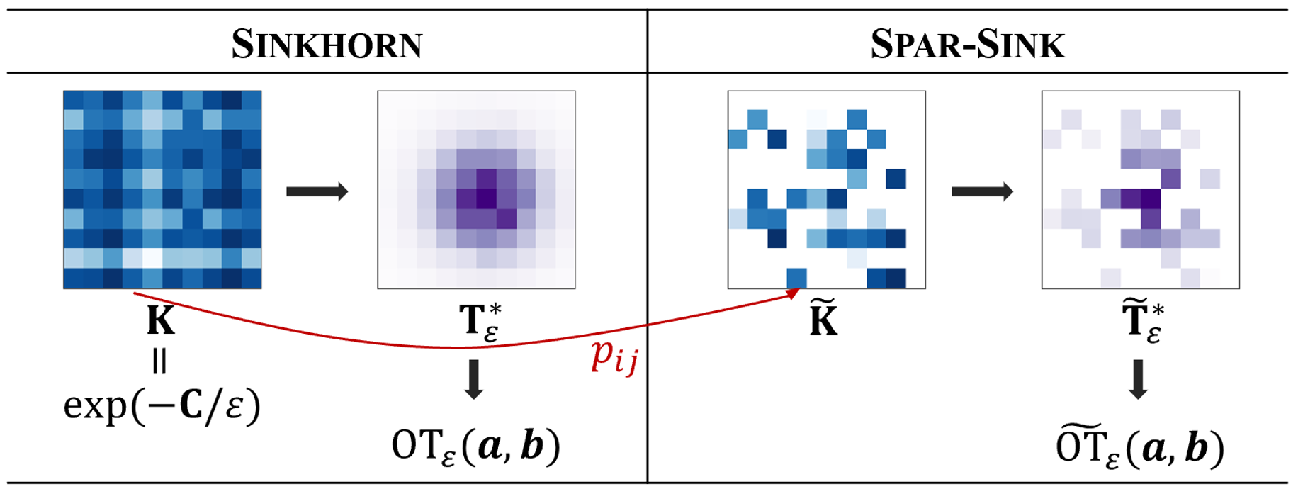
Figure 1: An illustration of the Sinkhorn algorithm (Left panel) and our Spar-Sink method (Right panel). The non-zero elements of each matrix are labeled with colors.

Consider the sampling probabilities $p_{ij}$. Note that the transportation loss in (6) can be written as a summation

$$\langle\mathbf{T}_{\varepsilon}^{\ast},\mathbf{C}\rangle=\sum_{i,j}{(T_{\varepsilon}^{\ast})}_{ij}C_{ij}.$$ (8)

According to (3), $\mathbf{T}_{\varepsilon}^{\ast}$ and $\mathbf{K}$ enjoy the same sparsity structure, that is, ${(T_{\varepsilon}^{\ast})}_{ij}=0$ if $K_{ij}=0$, as shown in Fig. 1. Thus, sampling elements from $\mathbf{K}$ is equivalent to sampling the corresponding terms from the summation (8). Following the idea of importance sampling, the optimal sampling probability $p_{ij}^{+}$ for $K_{ij}$ should be proportional to ${(T_{\varepsilon}^{\ast})}_{ij}C_{ij}$ from the perspective of variance-reduction. However, ${(T_{\varepsilon}^{\ast})}_{ij}$ is unknown beforehand, and thus $p_{ij}^{+}$ is impractical. Fortunately, there exists a natural upper bound for such a sampling probability. Based on the marginal constraints on $\mathbf{T}_{\varepsilon}^{\ast}$, we have ${(T_{\varepsilon}^{\ast})}_{ij}\leq a_{i}$ and ${(T_{\varepsilon}^{\ast})}_{ij}\leq b_{j}$. Moreover, we focus on the general scenario where the ground cost between supports is bounded, i.e., $C_{ij}\leq c_{0}$ for some constant $c_{0}>0$. Therefore, we have the upper bound

$${(T_{\varepsilon}^{\ast})}_{ij}C_{ij}\leq c_{0}\sqrt{a_{i}b_{j}}.$$

Such an inequality motivates us to use the sampling probability

$$p_{ij}=\frac{\sqrt{a_{i}b_{j}}}{\sum_{1\leq i,j\leq n}\sqrt{a_{i}b_{j}}},\quad 1\leq i,j\leq n.$$ (9)

Algorithm 3 summarizes the proposed algorithm for OT problems.

Algorithm 3 Spar-Sink algorithm for OT

1:Input: $\bm{a},\bm{b}\in\mathbb{R}_{+}^{n}$, $\mathbf{K}\in\mathbb{R}_{+}^{n\times n}$, $0<s<n^{2}$, $\varepsilon,\delta>0$

2:Construct $\widetilde{\mathbf{K}}$ according to (7) and (9)

3:Compute $\widetilde{\mathbf{T}}_{\varepsilon}^{\ast}=\textsc{SinkhornOT}(\widetilde{\mathbf{K}},\bm{a},\bm{b},\delta)$ by using Algorithm 1

4:Output: $\widetilde{\operatorname{OT}}_{\varepsilon}(\bm{a},\bm{b})=\langle\widetilde{\mathbf{T}}_{\varepsilon}^{\ast},\mathbf{C}\rangle-\varepsilon H(\widetilde{\mathbf{T}}_{\varepsilon}^{\ast})$

3.3 Importance Sparsification for UOT Problems

For unbalanced problems, we aim to approximate the entropic UOT distance

$$\operatorname{UOT}_{\lambda,\varepsilon}(\bm{a},\bm{b})=\langle\mathbf{T}_{\lambda,\varepsilon}^{\ast},\mathbf{C}\rangle+\lambda\mathrm{KL}(\mathbf{T}_{\lambda,\varepsilon}^{\ast}\mathbf{1}_{n}\|\bm{a})+\lambda\mathrm{KL}(\mathbf{T}_{\lambda,\varepsilon}^{\ast\top}\mathbf{1}_{n}\|\bm{b})-\varepsilon H(\mathbf{T}_{\lambda,\varepsilon}^{\ast}),$$ (10)

where $\mathbf{T}_{\lambda,\varepsilon}^{\ast}$ is the unique solution to (5). Again, we define $\bm{u}^{\ast},\bm{v}^{\ast}$ as the convergent scaling factors in Algorithm 2, such that $\mathbf{T}_{\lambda,\varepsilon}^{\ast}=\operatorname{diag}(\bm{u}^{\ast})\mathbf{K}\operatorname{diag}(\bm{v}^{\ast})$.

Similar to the former subsection, we apply the element-wise Poisson sampling to get an unbiased sparsification of $\mathbf{K}$. The formulation of $\widetilde{\mathbf{K}}$ is the same as the one in (7); however, the marginal constraints no longer hold, and thus the sampling probability differs.

Recall that our goal is to find an upper bound of $(T_{\lambda,\varepsilon}^{\ast})_{ij}C_{ij}$. According to the iteration steps in Algorithm 2, i.e., $(u_{i}^{\ast})^{(\lambda+\varepsilon)/\lambda}(\sum_{j=1}^{n}K_{ij}v_{j}^{\ast})=a_{i}$ and $(v_{j}^{\ast})^{(\lambda+\varepsilon)/\lambda}(\sum_{i=1}^{n}K_{ij}u_{i}^{\ast})=b_{j}$, we have

$$(u_{i}^{\ast})^{\frac{\lambda+\varepsilon}{\lambda}}K_{ij}v_{j}^{\ast}\leq a_{i},\quad u_{i}^{\ast}K_{ij}(v_{j}^{\ast})^{\frac{\lambda+\varepsilon}{\lambda}}\leq b_{j}\quad\Rightarrow\quad(u_{i}^{\ast})^{\frac{2\lambda+\varepsilon}{\lambda}}K_{ij}^{2}(v_{j}^{\ast})^{\frac{2\lambda+\varepsilon}{\lambda}}\leq a_{i}b_{j}$$

because scaling factors $\bm{u}^{\ast},\bm{v}^{\ast}$ are non-negative. This follows that

$$\left(T_{\lambda,\varepsilon}^{\ast}\right)_{ij}=u_{i}^{\ast}K_{ij}v_{j}^{\ast}\leq\left(a_{i}b_{j}\right)^{\frac{\lambda}{2\lambda+\varepsilon}}K_{ij}^{\frac{\varepsilon}{2\lambda+\varepsilon}}.$$

Under the scenario that $C_{ij}\leq c_{0}$, such an upper bound motivates us to sample with the probability

$$p_{ij}=\frac{(a_{i}b_{j})^{\frac{\lambda}{2\lambda+\varepsilon}}K_{ij}^{\frac{\varepsilon}{2\lambda+\varepsilon}}}{\sum_{1\leq i,j\leq n}(a_{i}b_{j})^{\frac{\lambda}{2\lambda+\varepsilon}}K_{ij}^{\frac{\varepsilon}{2\lambda+\varepsilon}}},\quad 1\leq i,j\leq n.$$ (11)

Note that when $\lambda\to\infty$, the sampling probability $p_{ij}$ defined by (11) degenerates to the one defined in (9). This is consistent with the fact that Algorithm 2 degenerates to Algorithm 1 when $\lambda\to\infty$. Algorithm 4 summarizes the proposed algorithm for UOT problems.

Algorithm 4 Spar-Sink algorithm for UOT

1:Input: $\bm{a},\bm{b}\in\mathbb{R}_{+}^{n}$, $\mathbf{K}\in\mathbb{R}_{+}^{n\times n}$, $0<s<n^{2}$, $\lambda,\varepsilon,\delta>0$

2:Construct $\widetilde{\mathbf{K}}$ according to (7) and (11)

3:Compute $\widetilde{\mathbf{T}}_{\lambda,\varepsilon}^{\ast}=\textsc{SinkhornUOT}(\widetilde{\mathbf{K}},\bm{a},\bm{b},\lambda,\varepsilon,\delta)$ by using Algorithm 2

4:Output: $\widetilde{\operatorname{UOT}}_{\lambda,\varepsilon}(\bm{a},\bm{b})=\langle\widetilde{\mathbf{T}}_{\lambda,\varepsilon}^{\ast},\mathbf{C}\rangle+\lambda\mathrm{KL}(\widetilde{\mathbf{T}}_{\lambda,\varepsilon}^{\ast}\mathbf{1}_{n}\|\bm{a})+\lambda\mathrm{KL}(\widetilde{\mathbf{T}}_{\lambda,\varepsilon}^{\ast\top}\mathbf{1}_{n}\|\bm{b})-\varepsilon H(\widetilde{\mathbf{T}}_{\lambda,\varepsilon}^{\ast})$

In this study, we further extend the Spar-Sink approach to approximate Wasserstein barycenters, by noticing that our importance sparsification mechanism is also applicable for accelerating the iterative Bregman projection algorithm (Benamou et al., 2015). Details for this extension are provided in the Appendix.

4 Theoretical Results

This section shows that the proposed estimators w.r.t. entropic OT and UOT distances are consistent under certain regularity conditions. All the proofs are detailed in the Appendix. Without loss of generality, we assume the supports of $\bm{a}$ and $\bm{b}$ are identical and $\varepsilon$ is relatively small. Then, the cost matrix $\mathbf{C}$ is symmetric, and the resulting kernel matrix $\mathbf{K}=\exp(-\mathbf{C}/\varepsilon)$ is positive definite.

Theorem 1

Under the regularity conditions (i) $\|\mathbf{K}\|_{2}\geq n^{\alpha}/c_{1}$ for constants $1/2<\alpha\leq 1$ and $c_{1}>0$, and the condition number of $\mathbf{K}$ is bounded by $c_{2}>0$, (ii) $p_{ij}^{*}\geq c_{3}{s}/{n^{2}}$ for $c_{3}>0$, and (iii) $s\geq c_{4}n^{3-2\alpha}\log^{4}(2n)$ for $c_{4}=8/(c_{3}\log^{4}(1+\epsilon))$ and $\epsilon>0$, as $n\to\infty$, the following result holds with probability approaching one that

$$\widetilde{\operatorname{OT}}_{\varepsilon}(\bm{a},\bm{b})\leq\operatorname{OT}_{\varepsilon}(\bm{a},\bm{b})+c_{5}\varepsilon\sqrt{n^{3-2\alpha}/s},$$ (12)

where $c_{5}>0$ is a constant depending on $c_{1}$, $c_{2}$, $c_{3}$, and $c_{4}$ only.

We discuss the regularity conditions in Theorem 1. Condition (i) is naturally established when $\varepsilon$ is relatively small. Indeed, non-diagonal entries of $\mathbf{K}$ go to zero quickly as the cost or distance increases, thus yielding a numerically sparse kernel matrix with a diagonal-like structure. Condition (ii) requires $p_{ij}$ to be of the order $O(1/n^{2})$, which can always be satisfied by combining the proposed sampling probability and uniform sampling probability linearly. Such a shrinkage strategy is common in subsampling literature, and we refer to Ma et al. (2015) and Yu et al. (2022) for more discussion. Condition (iii) implies that the subsample size should be large enough, especially when the signal in $\mathbf{K}$ is weak (i.e., $\alpha$ is small). Under the condition (iii), the upper bound of approximation error in (12) tends to zero in probability, which leads to the consistency of $\widetilde{\operatorname{OT}}_{\varepsilon}(\bm{a},\bm{b})$ w.r.t. the entropic OT distance. Moreover, consider a general case that $\|\mathbf{K}\|_{2}=O(n)$, i.e., $\alpha=1$, condition (iii) indicates us to select $s=\widetilde{O}(n)$ elements to construct the sparse sketch.

To analyze the UOT problem, we first normalize the kernel matrix $\mathbf{K}$ such that $\bm{1}_{n}^{\top}\mathbf{K}{\mathbf{1}_{n}}/n^{2}$ are bounded by $1/4$. This requirement can be naturally satisfied by rescaling the optimization problem (10) because $\bm{1}_{n}^{\top}\mathbf{K}{\mathbf{1}_{n}}/n^{2}\leq 1$. Then, the following result holds.

Theorem 2

Suppose the regularity conditions (i)—(iii) in Theorem 1 hold. Also suppose that (iv) $\varepsilon/\lambda\leq c_{6}$ and $\lambda\leq c_{7}n^{-c_{6}}$ for some constants $c_{6},c_{7}>0$, and (v) $\bm{a}^{\top}{\mathbf{1}_{n}}+\bm{b}^{\top}{\mathbf{1}_{n}}\leq\varepsilon/(2c_{7})$. As $n\to\infty$, the following result holds with probability approaching one that

$$\widetilde{\operatorname{UOT}}_{\lambda,\varepsilon}(\bm{a},\bm{b})\leq\operatorname{UOT}_{\lambda,\varepsilon}(\bm{a},\bm{b})+c_{8}\varepsilon\sqrt{n^{3-2\alpha}/s},$$ (13)

where $c_{8}>0$ is a constant depending on $c_{1}$, $c_{2}$, $c_{3}$, and $c_{4}$ only.

Consider the additional conditions in Theorem 2. Condition (iv) naturally holds when $\lambda=o(1)$ and $\varepsilon=O(\lambda)$. Condition (v) can also be satisfied by rescaling the finite measures. Theorem 2 shows the consistency of $\widetilde{\operatorname{UOT}}_{\lambda,\varepsilon}(\bm{a},\bm{b})$ w.r.t. the entropic UOT distance, and also requires $s$ to be at least of the order $\widetilde{O}(n)$.

The following theorem shows that the proposed Spar-Sink algorithm has the same number of iteration bound as the classical Sinkhorn algorithm up to a constant, for both OT and UOT problems. This result is a straightforward extension of the iteration bounds presented in Altschuler et al. (2017) and Pham et al. (2020).

Theorem 3

Suppose the Sinkhorn algorithm and Spar-Sink algorithm have the same settings of parameters. Under the conditions of Theorem 1 (resp. Theorem 2), both Algorithm 1 and Algorithm 3 (resp. Algorithm 2 and Algorithm 4) converge approximately within the same order of iterations in probability.

5 Simulations

In this section, we evaluate the performance of our proposed method (Spar-Sink) in both OT and UOT problems using synthetic data sets. We compare Spar-Sink with state-of-the-art variants of Sinkhorn regarding approximation accuracy and computational time, including: (i) Greenkhorn (Altschuler et al., 2017); (ii) Screenkhorn (Alaya et al., 2019); (iii) Nys-Sink (Altschuler et al., 2019); (iv) the naive random element-wise subsampling method in the Sinkhorn algorithm (Rand-Sink), which is similar to the proposed Spar-Sink method, except that the sampling probabilities for all the elements are equal to each other.

We set the stopping threshold $\delta=10^{-6}$ for all the algorithms considered in the experiments. The maximum number of iterations is set to be $5n$ for Greenkhorn and to be $10^{3}$ for all other methods. The decimation factor in Screenkhorn is taken as $3$. Other parameters are set by default according to the Python Optimal Transport toolbox (Flamary et al., 2021). All experiments are implemented on a server with 251GB RAM, 64 cores Intel(R) Xeon(R) Gold 5218 CPU and 4 GeForce RTX 3090 GPU. The implementation code is available at this link: https://github.com/Mengyu8042/Spar-Sink.

5.1 Approximation Performance

For the OT problem, the goal is to estimate the entropic OT distance between two empirical probability measures $\bm{a},\bm{b}\in\Delta^{n-1}$, i.e., $\operatorname{OT}_{\varepsilon}(\bm{a},\bm{b})$ defined in (2). These two measures share the same support points $\{\bm{x}_{i}\}_{i=1}^{n}$, where $\bm{x}_{i}\in\mathbb{R}^{d}$, $n=10^{3}$ and $d\in\{5,10,20,50\}$. We use the squared Euclidean cost matrix $\mathbf{C}$ such that $C_{ij}=\|\bm{x}_{i}-\bm{x}_{j}\|_{2}^{2}$ for $1\leq i,j\leq n$, and we take $\varepsilon\in\{10^{-1},10^{-2},10^{-3}\}$. In addition, we consider three scenarios for generating $\bm{a},\bm{b}$ and $\{\bm{x}_{i}\}_{i=1}^{n}$ as follows:

• $\bm{a},\bm{b}$ are empirical Gaussian distributions $N(\frac{1}{3},\frac{1}{20})$ and $N(\frac{1}{2},\frac{1}{20})$, respectively; $\bm{x}_{i}$’s are generated from multivariate uniform distribution over $(0,1)^{d}$, i.e., $\bm{x}_{i}\sim U(0,1)^{d}$;

• $\bm{a},\bm{b}$ are same to those in C1; $\bm{x}_{i}$’s are generated from multivariate Gaussian distribution, i.e., $\bm{x}_{i}\sim N(\mathbf{0}_{d},\mathbf{\Sigma})$ with $\Sigma_{jk}=0.5^{|j-k|}$ for $(j,k)\in[d]\times[d]$;

• $\bm{a},\bm{b}$ are empirical t-distributions with 5 degrees of freedom $t_{5}(\frac{1}{3},\frac{1}{20})$ and $t_{5}(\frac{1}{2},\frac{1}{20})$, respectively; $\bm{x}_{i}$’s are same to those in C1.

We first compare the subsampling-based approaches: Nys-Sink, Rand-Sink, and Spar-Sink (i.e., Algorithm 3). For the Rand-Sink and Spar-Sink methods, we set the expected subsample size $s=\{2,2^{2},2^{3},2^{4}\}\times s_{0}(n)$ with $s_{0}(n)=10^{-3}n\log^{4}(n)$, where $s_{0}(n)$ is set in the light of Theorem 1. For a fair comparison, we select $r=\lceil s/n\rceil$ columns in $\mathbf{K}$ for the Nys-Sink approach, such that the selected elements for the subsampling-based methods are roughly at the same size. To compare the approximation performance, we calculate the empirical relative mean absolute error (RMAE) for each estimator based on 100 replications, i.e.,

$$\operatorname{RMAE}^{(\operatorname{OT})}=\frac{1}{100}\sum_{i=1}^{100}\frac{|\widetilde{\operatorname{OT}}_{\varepsilon}^{(i)}-{\operatorname{OT}}_{\varepsilon}^{(i)}|}{{\operatorname{OT}}_{\varepsilon}^{(i)}},$$

where $\widetilde{\operatorname{OT}}_{\varepsilon}^{(i)}$ represents the estimator in the $i$th replication, and ${\operatorname{OT}}_{\varepsilon}^{(i)}$ is calculated using the classical Sinkhorn algorithm (i.e., Algorithm 1).

The results of $\operatorname{RMAE}^{(\operatorname{OT})}$ versus different subsample sizes $s$ are shown in Fig. 2. From Fig. 2, we observe that all the estimators result in smaller $\operatorname{RMAE}^{(\operatorname{OT})}$ as $s$ increases, and the proposed Spar-Sink method consistently outperforms the competitors. We also observe that Spar-Sink decreases faster than others in most cases, which indicates the proposed method has a relatively high convergence rate.

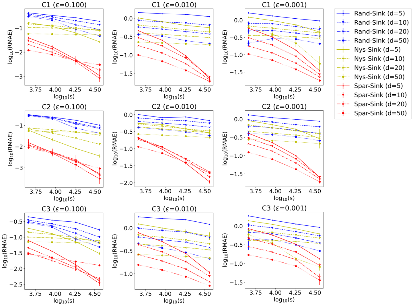
Figure 2: Comparison of subsampling-based methods w.r.t. $\operatorname{RMAE}^{(\operatorname{OT})}$ versus increasing $s$ (in log-log scale). Each row represents a different data generation pattern (C1—C3), and each column represents a different $\varepsilon$. Different methods are marked by different colors, respectively, and each line type represents a different dimension $d$. Vertical bars are the standard errors.

For the UOT problem shown in (5), we set the total mass of $\bm{a}$ and $\bm{b}$ to be 5 and 3, respectively. The regularization parameters are set to be $\varepsilon=0.1$ and $\lambda=0.1$. Other choices of parameters lead to similar results and are relegated to Appendix. Empirical results show the performance of the proposed method is robust to these parameters. The goal is to approximate the Wasserstein-Fisher-Rao distance, where the cost function is defined as $C_{ij}=-\log\left\{\cos_{+}^{2}\left(d_{ij}/(2\eta)\right)\right\}$ with Euclidean distance $d_{ij}=\|\bm{x}_{i}-\bm{x}_{j}\|_{2}$. Recall that the parameter $\eta$ controls the sparsity level of the kernel matrix $\mathbf{K}$, and a smaller $\eta$ is associated with a sparser $\mathbf{K}$. We take different values of $\eta$ such that there are around 70%, 50%, and 30% non-zero elements in $\mathbf{K}$, and these scenarios are denoted by R1, R2, and R3, respectively. Other settings are the same as those in OT problems.

For comparison, we calculate the empirical RMAE of approximating ${\operatorname{UOT}}_{\lambda,\varepsilon}(\bm{a},\bm{b})$ based on 100 replications, i.e.,

$$\operatorname{RMAE}^{(\operatorname{UOT})}=\frac{1}{100}\sum_{i=1}^{100}\frac{|\widetilde{\operatorname{UOT}}_{\lambda,\varepsilon}^{(i)}-{\operatorname{UOT}}_{\lambda,\varepsilon}^{(i)}|}{{\operatorname{UOT}}_{\lambda,\varepsilon}^{(i)}},$$

where $\widetilde{\operatorname{UOT}}_{\lambda,\varepsilon}^{(i)}$ represents the estimator in the $i$th replication, and ${\operatorname{UOT}}_{\lambda,\varepsilon}^{(i)}$ is calculated using the unbalanced Sinkhorn algorithm (i.e., Algorithm 2). The results of $\operatorname{RMAE}^{(\operatorname{UOT})}$ versus different $s$ are shown in Fig. 3, from which we observe that $\operatorname{RMAE}^{(\operatorname{UOT})}$ of both Rand-Sink and Nys-Sink methods decrease slowly with the increase of $s$, while Spar-Sink converges much faster. In general, the proposed Spar-Sink significantly outperforms the competitors under all circumstances. Such an observation indicates the proposed algorithm can select informative elements for the Sinkhorn algorithm, resulting in an asymptotically unbiased result with a relatively small estimation variance.

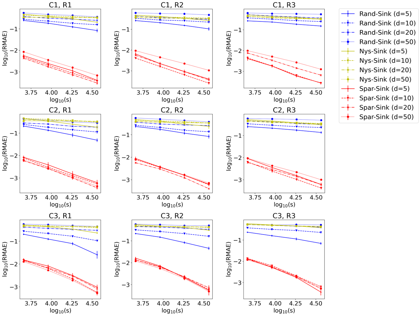
Figure 3: Comparison of subsampling-based methods w.r.t. $\operatorname{RMAE}^{(\operatorname{UOT})}$ versus increasing $s$ (in log-log scale). Each row represents a different data generation pattern (C1—C3), and each column represents a different sparsity ratio (R1—R3). Different methods are marked by different colors, respectively, and each line type represents a different dimension $d$. Vertical bars are the standard errors.

We now include the methods without subsampling, Greenkhorn and Screenkhorn, to comparison and fix the subsample parameter as $s=8s_{0}(n)$ for above subsampling-based approaches. We show their $\operatorname{RMAE}^{(\operatorname{OT})}$ versus increasing sample size $n$ under C1 in Fig. 4, where $n\in\{2^{2},2^{3},\ldots,2^{7}\}\times 10^{2}$. We omit the result of Screenkhorn in the case of $\varepsilon=10^{-3}$ as it fails to output a feasible solution when $\varepsilon$ is relatively small in our setup. From Fig. 4, we observe the proposed Spar-Sink method yields comparable errors to Greenkhorn and Screenkhorn for a relatively large $\varepsilon$, and its advantage turns prominent when $\varepsilon$ becomes small. Additionally, the approximation error of Spar-Sink converges asymptotically as $n$ increases, which is consistent with Theorem 1. We also show the convergence of $\operatorname{RMAE}^{(\operatorname{UOT})}$ versus increasing $n$ in the Appendix, and the results are in good agreement with Theorem 2.

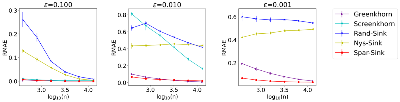
Figure 4: Comparison of different methods w.r.t. $\operatorname{RMAE}^{(\operatorname{OT})}$ versus $\log_{10}(n)$ under C1. Each subfigure represents a different $\varepsilon$, and each color marks a specific method. Vertical bars are the standard errors.

5.2 Computational Cost and CPU Time

Consider the computational cost of Algorithm 3. Constructing the sketch $\widetilde{\mathbf{K}}$ requires $O(n^{2})$ time, and such a step can be naturally paralleled. The matrix $\widetilde{\mathbf{K}}$ contains at most $s$ non-zero elements, and thus calculating $\widetilde{\mathbf{K}}\bm{v}$ and $\widetilde{\mathbf{K}}^{\top}\bm{u}$ takes $O(s)$ time. Therefore, the overall computational cost of Algorithm 3 is at the order of $O(n^{2}+Ls)$, which becomes $O(n^{2}+Ln)$ when $s=\widetilde{O}(n)$. Similarly, the computational cost of Algorithm 4 is at the order of $O(\mbox{nnz}(\mathbf{K})+Ln)$, where $\mbox{nnz}(\cdot)$ denotes the number of non-zero elements.

We compare the CPU time of the classical Sinkhorn algorithm and the variants of Sinkhorn for both OT and UOT problems in Fig. 5. The Rand-Sink method has similar computing time to Spar-Sink and is omitted for clarity. We choose $s=8s_{0}(n)$ for Spar-Sink and $r=\lceil s/n\rceil$ for Nys-Sink with $n\in\{2^{3},2^{4},\ldots,2^{8}\}\times 10^{2}$.

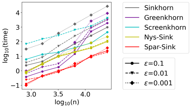
(a) CPU time (in seconds) for estimating the Wasserstein distance under C1.

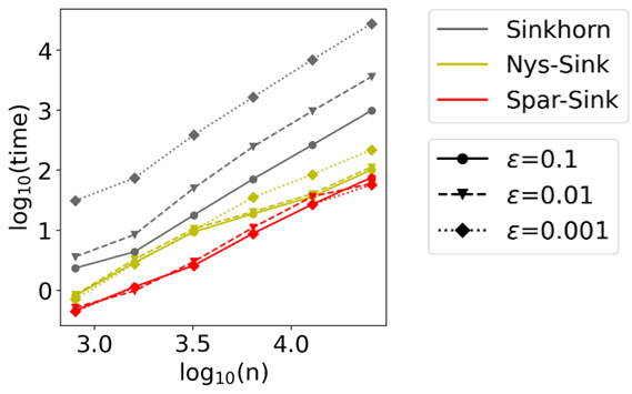
(b) CPU time (in seconds) for estimating the WFR distance under C1, R2.

Figure 5: Comparison of different methods w.r.t. computational time. Different methods are marked by different colors. Each line type represents a different value of $\varepsilon$.

In Fig. 5, we observe that Spar-Sink speeds up the Sinkhorn algorithm hundreds of times and also computes much faster than Greenkhorn and Screenkhorn, especially when $n$ is large enough. We also observe that a smaller value of $\varepsilon$ leads to a longer CPU time for the Sinkhorn algorithm. Such an observation is consistent with the results in Altschuler et al. (2017) and Pham et al. (2020), which showed the number of iterations for Sinkhorn increases as $\varepsilon$ decreases. In contrast, the effect of $\varepsilon$ on the CPU time is less significant for Spar-Sink. These observations indicate that the proposed algorithms are suitable for dealing with large-scale OT and UOT problems.

6 Echocardiogram Analysis

Echocardiography has been widely used to visualize myocardial motion due to its fast image acquisition, relatively low cost, and no side effects. Previous study has developed various echocardiology-based techniques to determine the ejection fraction (Ouyang et al., 2020), prognosticate cardiovascular disease (Zhang et al., 2021b), screen the cardiotoxicity (Bouhlel et al., 2020), among others. One fundamental task in echocardiogram data analysis is cardiac circle identification, which is necessary and crucial for downstream analysis. The cardiac cycle is the performance of the human heart from the beginning of one heartbeat to the beginning of the next. A single cycle consists of two basic periods, diastole and systole (Fye, 2015). Owing to the variation in cardiac activity caused by changes in loading and cardiac conditions, it is recommended to consider multiple cycles rather than only one representative cycle to perform measurements. However, this is not always done in clinical practice, given the tedious and laborious nature of human labeling. To obviate the heavy work for cardiologists, we propose an optimal transport method to automatically identify and visualize multiple cardiac cycles.

We consider an echocardiogram videos data set (Ouyang et al., 2020) containing 10,030 apical-four-chamber echocardiogram videos, each of which ranges from 24 to 1,002 frames with an average of 51 frames per second. A single frame is a gray-scale image of $112\times 112$ pixels. Each video is annotated with two separate time points representing the end-systole (ES) and the end-diastole (ED). Figure 6 gives a clip example of the echocardiogram videos data set.

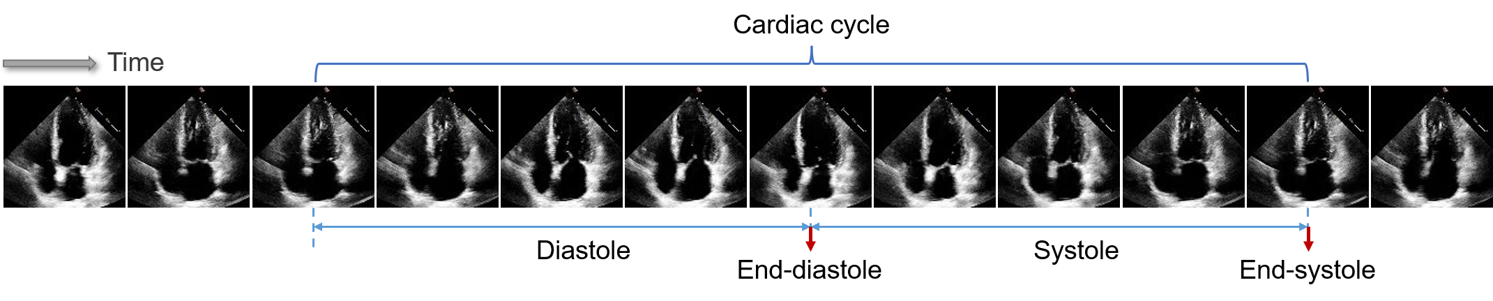
Figure 6: Echocardiogram videos data set visualization. Two basic periods, diastole and systole, form a cardiac cycle.

We propose identifying cardiac cycles using pairwise distances between the frames in an echocardiogram video. In particular, we use the normalized pixel gray levels of each frame as a mass distribution supported on $\mathbb{R}^{2}$, such that a lighter color is associated with a larger mass. We then use the Wasserstein-Fisher-Rao distance to measure the dissimilarity between each pair of frames. Compared to the Wasserstein distance, the WFR distance prevents long-range mass transportation and thus can achieve a balance between global transportation and local truncation. Intuitively, such a distance is more consistent with the characteristics of myocardial motion that the cardiac muscle would not move largely. To identify the cardiac cycles of an individual, we first compute the pairwise WFR distance matrix of his/her video, and then conduct a multidimensional scaling (MDS) for the distance matrix. However, computing the full WFR distance matrix using the classical Sinkhorn algorithm for a video of 200 frames requires nearly a hundred days. To alleviate the computational burden, we sample every other two frames (sampling period of 3) and then use our proposed Spar-Sink algorithm to approximate the pairwise WFR distances of the downsampled videos. The parameters are set to be $\varepsilon=0.01$, $\lambda=1$, $\eta=15$, and $s=8s_{0}(n)$. Empirical results show the performance is not sensitive to these parameters. Our CPU implementation requires only a few hours to calculate the distance matrix for one video. Further acceleration using GPU implementation is left for future research.

Figure 7 visualizes the distance matrices and the MDS results w.r.t. three individuals, respectively. Each dot in the MDS result represents a single frame, and the time points w.r.t. frames are denoted by different colors. By connecting the dots sequentially according to the time points, the cyclical nature of cardiac activities is clearly recovered. Moreover, we can make a preliminary assessment of one’s cardiac function from the pattern of these cardiac circles. For instance, by comparing with the first individual from the control group, we can see that the circle size differs in different cycles for the third individual with arrhythmia.

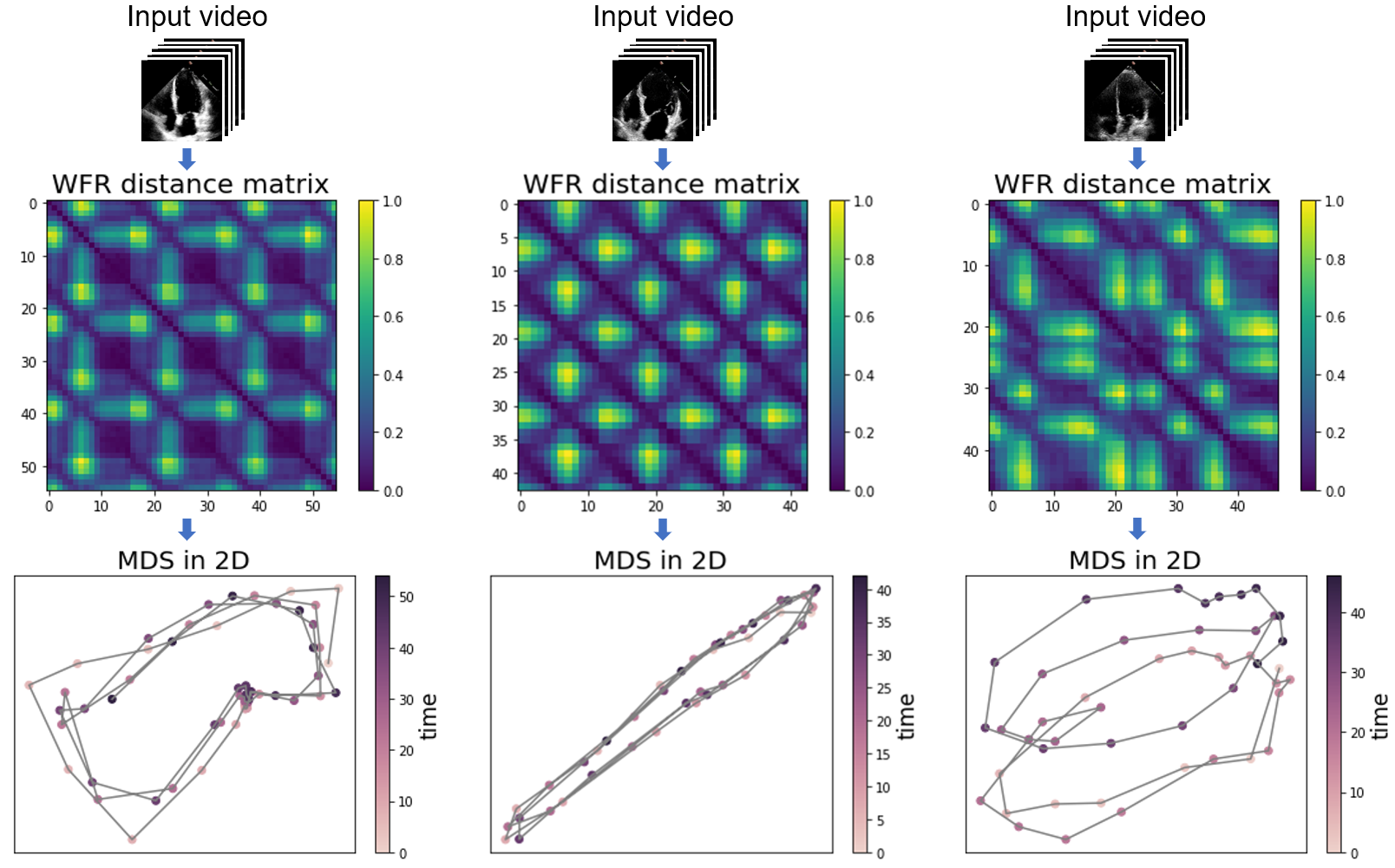
Figure 7: (From left to right) Each column is associated with an individual corresponding to a specific state of cardiac function, i.e., health, heart failure, and arrhythmia, respectively. (Top row) Input echocardiogram videos. (Middle row) Normalized WFR distance matrices computed by the Spar-Sink algorithm. (Bottom row) MDS in 2D: each point corresponds to a frame and is colored by the corresponding time iteration.

Beyond the intuitive visualization aforementioned, we are also interested in the accuracy of cycle prediction. Therefore, we consider the task of ED time point prediction. Specifically, for each video, we use the manually annotated ES and ED time points, $t_{ES}$ and $t_{ED}$, as the ground truth, and we aim to predict $t_{ED}$ using $t_{ES}$. Intuitively, in one cardiac cycle, the ED frame is the one that is most dissimilar to the ES frame. Following this line of thinking, we calculate the WFR distances between the ES frame and the other frames, respectively, within one cardiac cycle, and the predicted ED frame is the one that yields the largest WFR distance. After obtaining the prediction $\hat{t}_{ED}$, we define its error as

$$\text{Error}=\left|1-\frac{\hat{t}_{ED}-t_{ES}}{t_{ED}-t_{ES}}\right|.$$

A smaller error implies the prediction is closer to the ground truth.

(a) Original scale ($n=112\times 112$).
		$s=s_{0}(n)$	$s=2s_{0}(n)$	$s=2^{2}s_{0}(n)$	$s=2^{3}s_{0}(n)$	$n^{2}$
Nys-Sink	Error	0.49±0.23	0.44±0.27	0.31±0.28	0.32±0.22	-
	Time	370.30	522.37	662.71	831.01	-
Robust-NysSink	Error	0.47±0.34	0.41±0.25	0.34±0.18	0.33±0.17	-
	Time	376.01	509.58	664.50	838.61	-
Rand-Sink	Error	0.21±0.14	0.13±0.08	0.11±0.08	0.09±0.06	-
	Time	181.26	226.32	251.68	314.56	-
Spar-Sink	Error	0.09±0.06	0.07±0.05	0.06±0.05	0.06±0.04	-
	Time	210.69	262.89	302.9	357.46	-
Sinkhorn	Error	-	-	-	-	0.06±0.05
	Time	-	-	-	-	15649.31
(b) Mean-pooling with $2\times 2$ filters and stride 2 ($n=56\times 56$).
		$s=s_{0}(n)$	$s=2s_{0}(n)$	$s=2^{2}s_{0}(n)$	$s=2^{3}s_{0}(n)$	$n^{2}$
Nys-Sink	Error	0.78±0.21	0.64±0.26	0.55±0.27	0.45±0.26	-
	Time	40.51	46.97	51.46	59.54	-
Robust-NysSink	Error	0.79±0.31	0.61±0.27	0.50±0.24	0.43±0.22	-
	Time	40.75	46.11	50.08	56.20	-
Rand-Sink	Error	0.38±0.29	0.35±0.32	0.28±0.27	0.16±0.13	-
	Time	22.56	23.73	25.38	27.45	-
Spar-Sink	Error	0.30±0.21	0.14±0.11	0.11±0.09	0.11±0.09	-
	Time	24.34	27.24	28.59	32.43	-
Sinkhorn	Error	-	-	-	-	0.11±0.10
	Time	-	-	-	-	668.81

Table 1: Average errors (with standard deviations presented in footnotes) and CPU time (in seconds) for predicting the ED time point.

We calculate the WFR distances using the Sinkhorn algorithm, as well as three subsampling algorithms, i.e., Rand-Sink, Nys-Sink, and the proposed Spar-Sink algorithm, under different subsample sizes. Considering the potential outliers in real data, we also include a robust variant of Nys-Sink (Robust-NysSink) proposed by Le et al. (2021) for comparison. The results for 100 randomly selected videos are reported in Table 1. From panel (a) in Table 1, we observe that all these subsampling algorithms yield significantly less CPU time than the classical Sinkhorn algorithm. In addition, Spar-Sink is as accurate as Sinkhorn, while (Robust-)Nys-Sink and Rand-Sink yield much larger errors.

Another interesting question is how the proposed algorithm compares with pooling techniques, which are widely used in computer vision to accelerate computation (Boureau et al., 2010; Gong et al., 2014; Xu and Cheng, 2022). To answer this question, we reduce the size of the images from $112\times 112$ to $56\times 56$ using mean-pooling with $2\times 2$ filters and stride 2. We then compute the WFR distances on these pooled images. The results are provided in panel (b) of Table 1, from which we observe that all the algorithms require significantly less CPU time for the pooled images; however, the error increases. Again, the proposed Spar-Sink algorithm is the only one that yields the same error as the Sinkhorn algorithm. We also observe that compared to the Sinkhorn algorithm for pooled images (i.e., Sinkhorn in panel b), the Spar-Sink for original images (i.e., Spar-Sink in panel a) requires a shorter CPU time and yields more minor errors. Such an observation indicates that the proposed algorithm could be a better alternative for pooling strategy when calculating transport distances between large-scale images. In addition, one can also combine the pooling strategy with the proposed algorithm to further reduce CPU time without loss of accuracy.

Besides the application in echocardiogram analysis, we evaluate the Spar-Sink approach in two common machine learning applications: color transfer and generative modeling. The experimental results are presented in the Appendix, which provides additional evidence of the effectiveness of our proposed method.

7 Concluding Remarks

Realizing the natural upper bounds for unknown transport plans in (unbalanced) optimal transport problems, we propose a novel importance sparsification method to accelerate the Sinkhorn algorithm, approximating entropic OT and UOT distances in a unified framework. Theoretically, we show the consistency of proposed estimators under mild regularity conditions. Experiments on various synthetic data sets demonstrate the accuracy and efficiency of the proposed Spar-Sink approach. We also consider an echocardiogram video data set to illustrate its application in cardiac cycle identification, which shows our method offers a great trade-off between speed and accuracy.

Inspired by the work of Xie et al. (2020), Spar-Sink can be combined with the inexact proximal point method to approximate unregularized OT and UOT distances; further analyses are left to our future work. To handle potential outliers in practical applications, we also plan to extend the Spar-Sink method to the robust optimal transport framework (Le et al., 2021) in the future.

Acknowledgments and Disclosure of Funding

We thank the anonymous reviewers and Action Editor Michael Mahoney for their constructive comments that improved the quality of this paper. We also thank members of the Big Data Analytics Lab at the University of Georgia for their helpful comments. The authors would like to acknowledge the support from Beijing Municipal Natural Science Foundation No. 1232019, National Natural Science Foundation of China Grant No. 12101606, No. 12001042, No. 12271522, Renmin University of China research fund program for young scholars, and Beijing Institute of Technology research fund program for young scholars. Mengyu Li is supported by the Outstanding Innovative Talents Cultivation Funded Programs 2021 of Renmin University of China. The authors report there are no competing interests to declare.

Appendix A Importance Sparsification for Wasserstein Barycenters

In this section, we extend the Spar-Sink method to approximate fixed-support Wasserstein barycenters, which have been widely used in the machine learning community (Rabin et al., 2011; Benamou et al., 2015; Montesuma and Mboula, 2021).

A.1 Wasserstein Barycenters

Given a set of probability measures $\{\bm{b}_{1},\ldots,\bm{b}_{m}\}\subset\Delta^{n-1}$ and weights $\bm{w}\in\Delta^{m-1}$, a Wasserstein barycenter is computed by

$$\min_{\bm{q}\in\Delta^{n-1}}\sum_{k=1}^{m}w_{k}\operatorname{OT}(\bm{q},\bm{b}_{k}),$$ (14)

where $\operatorname{OT}(\bm{q},\bm{b}_{k})$ is defined in (1), associated with a prespecified distance matrix $\mathbf{C}_{k}\in\mathbb{R}_{+}^{n\times n}$ of the power $p$, for $k\in[m]$. Following the success of Cuturi (2013), the solution to (14) can also be approximated via entropic smoothing (Cuturi and Doucet, 2014); that is, replacing $\operatorname{OT}(\cdot)$ with $\operatorname{OT}_{\varepsilon}(\cdot)$ defined in (2) and leading to

$$\bm{q}_{\varepsilon}^{\ast}:=\arg\min_{\bm{q}\in\Delta^{n-1}}\sum_{k=1}^{m}w_{k}\operatorname{OT}_{\varepsilon}(\bm{q},\bm{b}_{k}).$$ (15)

By introducing kernel matrices $\mathbf{K}_{k}:=\exp(-\mathbf{C}_{k}/\varepsilon)$, the problem (15) can be rewritten as a weighted KL projection problem,

$$\min_{\mathbf{T}_{1},\ldots,\mathbf{T}_{m}\in\mathbb{R}_{+}^{n\times n}}\sum_{k=1}^{m}w_{k}\varepsilon\operatorname{KL}(\mathbf{T}_{k}\|\mathbf{K}_{k})\quad\text{s.t.}~{}\mathbf{T}_{k}^{\top}\mathbf{1}_{n}=\bm{b}_{k},k\in[m]~{}\text{and}~{}\mathbf{T}_{1}\mathbf{1}_{n}=\cdots=\mathbf{T}_{m}\mathbf{1}_{n}.$$

Here, the barycenter $\bm{q}$ is implied in the row marginals of transport plans as $\mathbf{T}_{k}\mathbf{1}_{n}=\bm{q}$ for $k\in[m]$. The authors of Benamou et al. (2015) proposed an iterative Bregman projection (IBP) algorithm, shown in Algorithm 5, to solve (15) effectively. In Algorithm 5, the notations $\odot$ and $\oslash$ represent element-wise multiplication and division, respectively.

Algorithm 5 IBP($\{\mathbf{K}_{k}\}_{k=1}^{m},\{\bm{b}_{k}\}_{k=1}^{m},\bm{w},\delta$)

1:Initialize: $t\leftarrow 0;\bm{q}^{(0)}\leftarrow\mathbf{1}_{n}/n;\bm{u}^{(0)}_{k}\leftarrow\mathbf{1}_{n},~{}\text{for}~{}k\in[m]$

2:repeat

3:     $t\leftarrow t+1$

4:     for $k=1\textbf{ to }m$: $~{}\bm{v}^{(t)}_{k}\leftarrow\bm{b}_{k}\oslash\mathbf{K}^{\top}_{k}\bm{u}^{(t-1)}_{k};\quad\bm{u}^{(t)}_{k}\leftarrow\bm{q}^{(t-1)}\oslash\mathbf{K}_{k}\bm{v}^{(t)}_{k}$

5:     $\bm{q}^{(t)}\leftarrow(\mathbf{K}_{1}\bm{v}_{1}^{(t)})^{w_{1}}\odot\cdots\odot(\mathbf{K}_{m}\bm{v}_{m}^{(t)})^{w_{m}}$

6:until $\|\bm{q}^{(t)}-\bm{q}^{(t-1)}\|_{1}\leq\delta$

7:Output: $\bm{q}^{(t)}$

A.2 Proposed Algorithm

As a generalized Sinkhorn algorithm, the IBP algorithm needs to compute matrix-vector multiplications w.r.t. $\mathbf{K}_{1},\ldots,\mathbf{K}_{m}$ at each iteration. Analogous to the idea of Spar-Sink, we approximate the dense kernel matrices with sparse sketches $\widetilde{\mathbf{K}}_{1},\ldots,\widetilde{\mathbf{K}}_{m}$ and propose a new Spar-IBP algorithm.

Recall that $\widetilde{\mathbf{K}}_{k}$ is defined by

$$\widetilde{K}_{k,ij}=\begin{cases}K_{k,ij}/p^{\ast}_{k,ij}&\text{ with prob. }p^{\ast}_{k,ij}=\min\left(1,sp_{k,ij}\right)\\ 0&\text{ otherwise. }\end{cases}$$ (16)

According to the principle of importance sampling, the sampling probability $p_{k,ij}$ should be proportional to $\sqrt{q^{\ast}_{\varepsilon,i}b_{k,j}}$. Unfortunately, such a probability depends on the unknown barycenter. To bypass the obstacle, we propose to replace the unknown $\bm{q}_{\varepsilon}^{\ast}$ with the initial value $\bm{q}^{(0)}=\mathbf{1}_{n}/n$, which implies the elements in the same column of $\widetilde{\mathbf{K}}_{k}$ have the equal probability to be selected. Such a procedure is reasonable considering it is common that the prior information of the barycenter is inaccessible.

Algorithm 6 Spar-IBP algorithm for Wasserstein barycenters

1:Input: $\{\mathbf{K}_{k}\}_{k=1}^{m}\subset\mathbb{R}_{+}^{n\times n}$, $\{\bm{b}_{k}\}_{k=1}^{m}\subset\Delta^{n-1}$, $\bm{w}\in\Delta^{m-1}$, $0<s<n^{2}$, $\delta>0$

2:For $k\in[m]$, construct $\widetilde{\mathbf{K}}_{k}$ according to (16) with

$$p_{k,ij}=\frac{\sqrt{b_{k,j}}}{n\sum_{j=1}^{n}\sqrt{b_{k,j}}},\quad 1\leq i,j\leq n$$

3:Compute $\widetilde{\bm{q}}_{\varepsilon}^{\ast}=\textsc{IBP}(\{\widetilde{\mathbf{K}}_{k}\}_{k=1}^{m},\{\bm{b}_{k}\}_{k=1}^{m},\bm{w},\delta)$ by using Algorithm 5

4:Output: $\widetilde{\bm{q}}_{\varepsilon}^{\ast}$

Algorithm 6 details the proposed Spar-IBP algorithm for approximating Wasserstein barycenters. Compared to Algorithm 5, it reduces the computational complexity of each iteration from $O(mn^{2})$ to $O(ms)$.

Appendix B Technical Details

In this appendix, we provide technical details of the theoretical results stated within the manuscript.

B.1 Proof of Theorem 1

Recall that Sinkhorn algorithm aims to solve the following optimization problem

$$\mathbf{T}_{\varepsilon}^{\ast}=\min_{\mathbf{T}\in\mathcal{U}(\bm{a},\bm{b})}\langle\mathbf{T},\mathbf{C}\rangle-\varepsilon H(\mathbf{T}).$$ (17)

The dual problem of (17) is

$$\max_{\bm{\alpha}\in\mathbb{R}^{n},\bm{\beta}\in\mathbb{R}^{n}}f(\bm{\alpha},\bm{\beta}):=\bm{a}^{\top}\bm{\alpha}+\bm{b}^{\top}\bm{\beta}-\varepsilon(e^{\bm{\alpha}/\varepsilon})^{\top}\mathbf{K}e^{\bm{\beta}/\varepsilon}+\varepsilon,$$ (18)

where $\mathbf{K}=\exp(-\mathbf{C}/\varepsilon)$ is the kernel matrix, and $\bm{\alpha},\bm{\beta}\in\mathbb{R}^{n}$ are dual variables. As been defined in Section 3.2, $\widetilde{\mathbf{T}}_{\varepsilon}^{\ast}$ is the sparsification counterpart to (17), and the corresponding dual problem becomes

$$\max_{\bm{\alpha}\in\mathbb{R}^{n},\bm{\beta}\in\mathbb{R}^{n}}\tilde{f}(\bm{\alpha},\bm{\beta}):=\bm{a}^{\top}\bm{\alpha}+\bm{b}^{\top}\bm{\beta}-\varepsilon(e^{\bm{\alpha}/\varepsilon})^{\top}\widetilde{\mathbf{K}}e^{\bm{\beta}/\varepsilon}+\varepsilon,$$ (19)

which replaces $\mathbf{K}$ in (18) with its sparse sketch $\widetilde{\mathbf{K}}$.

To prove the Theorem 1, we first introduce several lemmas.

Lemma 4

Suppose both $\mathbf{K}$ and $\widetilde{\mathbf{K}}$ are positive definite. Further suppose the condition number of $\mathbf{K}$ and $\widetilde{\mathbf{K}}$ are bounded by $c_{2}$ and $c_{2}^{\prime}$, respectively. Let $(\bm{\alpha}^{*},\bm{\beta}^{*})$ be the solution to (18), and $(\bar{\bm{\alpha}},\bar{\bm{\beta}})$ be the solution to (19). It follows that

$$|f(\bm{\alpha}^{*},\bm{\beta}^{*})-f(\bar{\bm{\alpha}},\bar{\bm{\beta}})|\leq\varepsilon\left(c_{2}+c_{2}^{\prime}\left|1-\frac{\|\widetilde{\mathbf{K}}-\mathbf{K}\|_{2}}{\|\mathbf{K}\|_{2}}\right|^{-1}\right)\frac{\|\widetilde{\mathbf{K}}-\mathbf{K}\|_{2}}{\|\mathbf{K}\|_{2}},$$ (20)

where $\|\cdot\|_{2}$ denotes the spectral norm (i.e., the maximal singular value) of a matrix.

Proof  First, we establish the following inequality:

$$|f(\bm{\alpha}^{*},\bm{\beta}^{*})-f(\bar{\bm{\alpha}},\bar{\bm{\beta}})|\leq|f(\bm{\alpha}^{*},\bm{\beta}^{*})-\tilde{f}({\bm{\alpha}}^{*},{\bm{\beta}}^{*})|+|\tilde{f}(\bar{\bm{\alpha}},\bar{\bm{\beta}})-f(\bar{\bm{\alpha}},\bar{\bm{\beta}})|.$$ (21)

By the definitions of $\bm{\alpha}^{*},\bm{\beta}^{*},\bar{\bm{\alpha}},\bar{\bm{\beta}}$, it holds that

$$\tilde{f}(\bar{\bm{\alpha}},\bar{\bm{\beta}})\geq\tilde{f}(\bm{\alpha}^{*},\bm{\beta}^{*}),\quad f(\bm{\alpha}^{*},\bm{\beta}^{*})\geq f(\bar{\bm{\alpha}},\bar{\bm{\beta}}).$$

We consider the following two cases:

• $\text{Case 1. }f(\bm{\alpha}^{*},\bm{\beta}^{*})\geq\tilde{f}(\bar{\bm{\alpha}},\bar{\bm{\beta}})$;

• $\text{Case 2. }f(\bm{\alpha}^{*},\bm{\beta}^{*})<\tilde{f}(\bar{\bm{\alpha}},\bar{\bm{\beta}})$.

For Case 1, it holds that $0\leq f(\bm{\alpha}^{*},\bm{\beta}^{*})-\tilde{f}(\bar{\bm{\alpha}},\bar{\bm{\beta}})\leq f(\bm{\alpha}^{*},\bm{\beta}^{*})-\tilde{f}(\bm{\alpha}^{*},\bm{\beta}^{*})$, and thus $|f(\bm{\alpha}^{*},\bm{\beta}^{*})-\tilde{f}(\bar{\bm{\alpha}},\bar{\bm{\beta}})|\leq|f(\bm{\alpha}^{*},\bm{\beta}^{*})-\tilde{f}(\bm{\alpha}^{*},\bm{\beta}^{*})|$, which leads to (21) by combining the triangle inequality

$$|f(\bm{\alpha}^{*},\bm{\beta}^{*})-f(\bar{\bm{\alpha}},\bar{\bm{\beta}})|\leq|f(\bm{\alpha}^{*},\bm{\beta}^{*})-\tilde{f}(\bar{\bm{\alpha}},\bar{\bm{\beta}})|+|\tilde{f}(\bar{\bm{\alpha}},\bar{\bm{\beta}})-f(\bar{\bm{\alpha}},\bar{\bm{\beta}})|.$$

For Case 2, (i) when $f(\bar{\bm{\alpha}},\bar{\bm{\beta}})\leq\tilde{f}({\bm{\alpha}}^{*},{\bm{\beta}}^{*})$, it holds that $0\leq\tilde{f}({\bm{\alpha}}^{*},{\bm{\beta}}^{*})-f(\bar{\bm{\alpha}},\bar{\bm{\beta}})\leq\tilde{f}(\bar{\bm{\alpha}},\bar{\bm{\beta}})-f(\bar{\bm{\alpha}},\bar{\bm{\beta}})$, and thus $|\tilde{f}({\bm{\alpha}}^{*},{\bm{\beta}}^{*})-f(\bar{\bm{\alpha}},\bar{\bm{\beta}})|\leq|\tilde{f}(\bar{\bm{\alpha}},\bar{\bm{\beta}})-f(\bar{\bm{\alpha}},\bar{\bm{\beta}})|$, which leads to (21) by combining the triangle inequality

$$|f(\bm{\alpha}^{*},\bm{\beta}^{*})-f(\bar{\bm{\alpha}},\bar{\bm{\beta}})|\leq|f(\bm{\alpha}^{*},\bm{\beta}^{*})-\tilde{f}(\bm{\alpha}^{*},\bm{\beta}^{*})|+|\tilde{f}(\bm{\alpha}^{*},\bm{\beta}^{*})-f(\bar{\bm{\alpha}},\bar{\bm{\beta}})|.$$

(ii) When $f(\bar{\bm{\alpha}},\bar{\bm{\beta}})>\tilde{f}({\bm{\alpha}}^{*},{\bm{\beta}}^{*})$, we have $|f(\bm{\alpha}^{*},\bm{\beta}^{*})-f(\bar{\bm{\alpha}},\bar{\bm{\beta}})|\leq|f(\bm{\alpha}^{*},\bm{\beta}^{*})-\tilde{f}({\bm{\alpha}}^{*},{\bm{\beta}}^{*})|$; then (21) establishes because $|\tilde{f}(\bar{\bm{\alpha}},\bar{\bm{\beta}})-f(\bar{\bm{\alpha}},\bar{\bm{\beta}})|\geq 0$.

Consequently, we conclude the inequality (21) by combining Cases 1 and 2.

Next, we provide an upper bound for the right-hand side of (21). Simple calculation yields that

$$|f(\bm{\alpha}^{*},\bm{\beta}^{*})-\tilde{f}(\bm{\alpha}^{*},\bm{\beta}^{*})|= |\varepsilon\langle e^{\bm{\alpha}^{*}/\varepsilon},(\widetilde{\mathbf{K}}-\mathbf{K})e^{\bm{\beta}^{*}/\varepsilon}\rangle|$$

$$= \varepsilon|\textrm{tr}\{(e^{\bm{\alpha}^{*}/\varepsilon})^{\top}(\widetilde{\mathbf{K}}-\mathbf{K})\mathbf{K}^{-1}\mathbf{K}e^{\bm{\beta}^{*}/\varepsilon}\}|.$$ (22)

As $(\bm{\alpha}^{*},\bm{\beta}^{*})$ is the optimal solution to $f(\bm{\alpha},\bm{\beta})$, the first order condition implies that

$$\textrm{tr}\{\mathbf{K}e^{\bm{\beta}^{*}/\varepsilon}(e^{\bm{\alpha}^{*}/\varepsilon})^{\top}\}=(e^{\bm{\alpha}^{*}/\varepsilon})^{\top}\mathbf{K}e^{\bm{\beta}^{*}/\varepsilon}=1.$$

Moreover, one can find that

$$\|(\widetilde{\mathbf{K}}-\mathbf{K})\mathbf{K}^{-1}\|_{2}\leq\|\widetilde{\mathbf{K}}-\mathbf{K}\|_{2}/\lambda_{\min}(\mathbf{K}),$$

where $\lambda_{\min}(\mathbf{K})$ is the minimal eigenvalue of $\mathbf{K}$. For notation simplicity, denote $\mathbf{G}=(\widetilde{\mathbf{K}}-\mathbf{K})\mathbf{K}^{-1}$ and $\mathbf{H}=\mathbf{K}e^{\bm{\beta}^{*}/\varepsilon}(e^{\bm{\alpha}^{*}/\varepsilon})^{\top}$. Let $\bm{h}_{j}$ be the $j$th column of $\mathbf{H}$, and $\bm{e}_{j}$ be the unit vector with $j$th element being one. Simple linear algebra yields that

$$|\textrm{tr}(\mathbf{G}\mathbf{H})|\leq\sum_{j=1}^{n}{\bm{e}}_{j}^{\top}|\mathbf{G}\bm{h}_{j}|\leq\sum_{j=1}^{n}\|\mathbf{G}\|_{2}\|\bm{h}_{j}\|_{2},$$

where the last equation comes from the Cauchy-Schwarz inequality. Also note that $\mathbf{H}$ is a rank-one matrix; therefore, (22) can be bounded by

$$|f(\bm{\alpha}^{*},\bm{\beta}^{*})-\tilde{f}(\bm{\alpha}^{*},\bm{\beta}^{*})| \leq\varepsilon\|\widetilde{\mathbf{K}}-\mathbf{K}\|_{2}|\textrm{tr}\{\mathbf{K}e^{\bm{\beta}^{*}/\varepsilon}(e^{\bm{\alpha}^{*}/\varepsilon})^{\top}\}|/\lambda_{\min}(\mathbf{K})$$

$$=\varepsilon\|\widetilde{\mathbf{K}}-\mathbf{K}\|_{2}/\lambda_{\min}(\mathbf{K})$$

$$\leq\varepsilon c_{2}\|\widetilde{\mathbf{K}}-\mathbf{K}\|_{2}/\|\mathbf{K}\|_{2}.$$ (23)

Using the same procedure, we obtain that

$$|f({\bm{\bar{\alpha}}},\bm{\bar{\beta}})-\tilde{f}(\bm{\bar{\alpha}},\bm{\bar{\beta}})|= |\varepsilon\langle e^{{\bm{\bar{\alpha}}}/\varepsilon},(\widetilde{\mathbf{K}}-\mathbf{K})e^{{\bm{\bar{\beta}}}/\varepsilon}\rangle|$$

$$= \varepsilon|\langle e^{{\bm{\bar{\alpha}}}/\varepsilon},(\widetilde{\mathbf{K}}-\mathbf{K})\widetilde{\mathbf{K}}^{-1}\widetilde{\mathbf{K}}e^{{\bm{\bar{\beta}}}/\varepsilon}\rangle|$$

$$\leq \varepsilon\|(\widetilde{\mathbf{K}}-\mathbf{K})\widetilde{\mathbf{K}}^{-1}\|_{2}|\textrm{tr}\{\widetilde{\mathbf{K}}e^{\bar{\bm{\beta}}/\varepsilon}(e^{\bar{\bm{\alpha}}/\varepsilon})^{\top}\}|.$$ (24)

As $(\bar{\bm{\alpha}},\bar{\bm{\beta}})$ is the optimal solution to $\tilde{f}(\bm{\alpha},\bm{\beta})$, the first order condition implies that

$$\textrm{tr}\{\widetilde{\mathbf{K}}e^{\bar{\bm{\beta}}/\varepsilon}(e^{\bar{\bm{\alpha}}/\varepsilon})^{\top}\}=(e^{\bar{\bm{\alpha}}/\varepsilon})^{\top}\widetilde{\mathbf{K}}e^{\bar{\bm{\beta}}/\varepsilon}=1.$$

Furthermore, simple calculation yields that

$$\|(\widetilde{\mathbf{K}}-\mathbf{K})\widetilde{\mathbf{K}}^{-1}\|_{2} \leq\|\widetilde{\mathbf{K}}-\mathbf{K}\|_{2}/\lambda_{\min}(\widetilde{\mathbf{K}})$$

$$\leq c_{2}^{\prime}\|\widetilde{\mathbf{K}}-\mathbf{K}\|_{2}/\|\widetilde{\mathbf{K}}\|_{2}$$

$$=c_{2}^{\prime}\frac{\|\widetilde{\mathbf{K}}-\mathbf{K}\|_{2}}{\|\mathbf{K}\|_{2}}\frac{\|\mathbf{K}\|_{2}}{\|\widetilde{\mathbf{K}}\|_{2}}$$

$$\leq c_{2}^{\prime}\frac{\|\widetilde{\mathbf{K}}-\mathbf{K}\|_{2}}{\|\mathbf{K}\|_{2}}\frac{\|\mathbf{K}\|_{2}}{|\|\mathbf{K}\|_{2}-\|\widetilde{\mathbf{K}}-\mathbf{K}\|_{2}|}$$

$$=c_{2}^{\prime}\frac{\|\widetilde{\mathbf{K}}-\mathbf{K}\|_{2}}{\|\mathbf{K}\|_{2}}\left|1-\frac{\|\widetilde{\mathbf{K}}-\mathbf{K}\|_{2}}{\|\mathbf{K}\|_{2}}\right|^{-1},$$

where the last inequality comes from the triangle inequality. Therefore, (24) satisfies that

$$|f(\bar{\bm{\alpha}},\bar{\bm{\beta}})-\tilde{f}(\bar{\bm{\alpha}},\bar{\bm{\beta}})|\leq\varepsilon c_{2}^{\prime}\frac{\|\widetilde{\mathbf{K}}-\mathbf{K}\|_{2}}{\|\mathbf{K}\|_{2}}\left|1-\frac{\|\widetilde{\mathbf{K}}-\mathbf{K}\|_{2}}{\|\mathbf{K}\|_{2}}\right|^{-1}.$$ (25)

Combining (21), (23), and (25), the result follows.  

Now we show that under some mild conditions, our subsampling procedure yields a relatively small difference between $\widetilde{\mathbf{K}}$ and $\mathbf{K}$.

Lemma 5

Suppose the regularity conditions (i)—(iii) in Theorem 1 hold. For any $\epsilon>0$ and $n>76$, we have

$$\mathbb{P}\left(\frac{\|\widetilde{\mathbf{K}}-\mathbf{K}\|_{2}}{\|\mathbf{K}\|_{2}}\geq{2\sqrt{2}(2+\epsilon)}c_{1}\sqrt{\frac{n^{3-2\alpha}}{c_{3}s}}\right)<2\exp\left(-\frac{16}{\epsilon^{4}}\log^{4}(n)\right).$$ (26)

Proof  By the definition of $\mathbf{K}$, one can find that $K_{ij}\leq 1$ for any $i,j=1,\ldots,n$. Simple calculation yields that

$$\mathbb{E}\left(\|\mathbf{K}\|_{2}^{-1}\widetilde{K}_{ij}\right) =\|\mathbf{K}\|_{2}^{-1}K_{ij},$$

$$\textrm{Var}\left(\|\mathbf{K}\|_{2}^{-1}\widetilde{K}_{ij}\right) <\frac{K_{ij}^{2}}{p_{ij}^{*}\|\mathbf{K}\|_{2}^{2}}\leq\frac{1}{p_{ij}^{*}\|\mathbf{K}\|_{2}^{2}}\leq\frac{n^{2}}{c_{3}s\|\mathbf{K}\|_{2}^{2}}.$$

Also note that $\|\mathbf{K}\|_{2}^{-1}\widetilde{K}_{ij}$ lies between $0$ and $(p_{ij}^{*}\|\mathbf{K}\|_{2})^{-1}$ for any $(i,j)$th entry. Thus, $\|\mathbf{K}\|_{2}^{-1}\widetilde{K}_{ij}$ takes the value in an interval of length not larger than $L$, with

$$L:=\frac{n^{2}}{c_{3}s\|\mathbf{K}\|_{2}} \leq\sqrt{\frac{n^{3-2\alpha}}{2c_{3}s}}\times\sqrt{\frac{n^{2}}{c_{3}s\|\mathbf{K}\|_{2}^{2}}}\times\sqrt{2n}$$

$$\leq\left(\frac{\log(1+\epsilon)}{2\log(2n)}\right)^{2}\times\sqrt{\frac{n^{2}}{c_{3}s\|\mathbf{K}\|_{2}^{2}}}\times\sqrt{2n},$$

where $L$ is defined according to the condition (ii), and the last inequality holds under the condition (iii). Therefore, by applying Theorem 3.1 in Achlioptas and Mcsherry (2007) on $\|\mathbf{K}\|_{2}^{-1}\widetilde{\mathbf{K}}$, we have

$$\mathbb{P}\left(\frac{\|\widetilde{\mathbf{K}}-\mathbf{K}\|_{2}}{\|\mathbf{K}\|_{2}}\geq 2(2+\epsilon)\sqrt{\frac{{2n^{3}}}{c_{3}s\|\mathbf{K}\|_{2}^{2}}}\right)<2\exp\left(-\frac{16}{\epsilon^{4}}\log^{4}(n)\right).$$ (27)

Further, combining (27) with the condition (i) results in the inequality (26).  

Finally, we prove the Theorem 1 in the manuscript.

Proof  From Lemma 5, it is straightforward to see that $\|\mathbf{K}\|_{2}^{-1}\widetilde{\mathbf{K}}\to\|\mathbf{K}\|_{2}^{-1}\mathbf{K}$ in probability. Thus, $\widetilde{\mathbf{K}}$ tends to be positive definite since $\mathbf{K}$ is a positive definite kernel matrix, and it holds that $c_{2}^{\prime}\to c_{2}$. Note that $n^{3-2\alpha}/s\to 0$ as $n\to\infty$, it is easy to see that when $n$ is large enough, we have

$$c^{\prime}\sqrt{n^{3-2\alpha}/s}\leq 1/2~{}~{}\text{with}~{}~{}c^{\prime}=2\sqrt{2}(2+\epsilon)c_{1}/\sqrt{c_{3}},$$

and this implies $(1+|1-c^{\prime}\sqrt{n^{3-2\alpha}/s}|^{-1})\leq 3$. Combining Lemmas 4 and 5, the result follows.  

B.2 Proof of Theorem 2

Now we focus on the entropy-regularized UOT problem, whose dual problem is

$$\max_{\bm{\alpha}\in\mathbb{R}^{n},\bm{\beta}\in\mathbb{R}^{n}}f_{u}(\bm{\alpha},\bm{\beta}):=\bm{a}^{\top}{\mathbf{1}_{n}}-\lambda\bm{a}^{\top}e^{-\bm{\alpha}/\lambda}+\bm{b}^{\top}{\mathbf{1}_{n}}-\lambda\bm{b}^{\top}e^{-\bm{\beta}/\lambda}-\varepsilon(e^{\bm{\alpha}/\varepsilon})^{\top}\mathbf{K}e^{\bm{\beta}/\varepsilon}.$$ (28)

Let

$$\max_{\bm{\alpha}\in\mathbb{R}^{n},\bm{\beta}\in\mathbb{R}^{n}}\tilde{f}_{u}(\bm{\alpha},\bm{\beta}):=\bm{a}^{\top}{\mathbf{1}_{n}}-\lambda\bm{a}^{\top}e^{-\bm{\alpha}/\lambda}+\bm{b}^{\top}{\mathbf{1}_{n}}-\lambda\bm{b}^{\top}e^{-\bm{\beta}/\lambda}-\varepsilon(e^{\bm{\alpha}/\varepsilon})^{\top}\widetilde{\mathbf{K}}e^{\bm{\beta}/\varepsilon}$$ (29)

be the sparsification counterpart to (28), which replaces $\mathbf{K}$ in (28) with its sparse sketch $\widetilde{\mathbf{K}}$. Apparently, it is the dual problem for the entropic UOT problem with kernel $\widetilde{\mathbf{K}}$. The following lemma holds by similar procedures as in Lemma 4.

Lemma 6

Suppose the regularity conditions (iv) and (v) in Theorem 2 hold. Further suppose both $\mathbf{K}$ and $\widetilde{\mathbf{K}}$ are positive definite, their condition numbers are respectively bounded by $c_{2}$ and $c_{2}^{\prime}$, and $\bm{1}_{n}^{\top}(\mathbf{K}-\widetilde{\mathbf{K}}){\mathbf{1}_{n}}/n^{2}\leq 1/4$. Let $(\bm{\alpha}^{*},\bm{\beta}^{*})$ be the solution to (28), and $(\bar{\bm{\alpha}},\bar{\bm{\beta}})$ be the solution to (29). It follows that

$$|f_{u}(\bm{\alpha}^{*},\bm{\beta}^{*})-f_{u}(\bar{\bm{\alpha}},\bar{\bm{\beta}})|\leq\varepsilon\left(c_{2}+c_{2}^{\prime}\left|1-\frac{\|\widetilde{\mathbf{K}}-\mathbf{K}\|_{2}}{\|\mathbf{K}\|_{2}}\right|^{-1}\right)\frac{\|\widetilde{\mathbf{K}}-\mathbf{K}\|_{2}}{\|\mathbf{K}\|_{2}}.$$

Proof  The proof is similar to that of Lemma 4. By the definitions of $\bm{\alpha}^{*},\bm{\beta}^{*},\bar{\bm{\alpha}},\bar{\bm{\beta}}$ and the triangle inequality, it holds that

$$|f_{u}(\bm{\alpha}^{*},\bm{\beta}^{*})-f_{u}(\bar{\bm{\alpha}},\bar{\bm{\beta}})|\leq|f_{u}(\bm{\alpha}^{*},\bm{\beta}^{*})-\tilde{f}_{u}({\bm{\alpha}}^{*},{\bm{\beta}}^{*})|+|\tilde{f}_{u}(\bar{\bm{\alpha}},\bar{\bm{\beta}})-f_{u}(\bar{\bm{\alpha}},\bar{\bm{\beta}})|.$$ (30)

For the first term in the right-hand side of (30), simple calculation yields that

$$|f_{u}(\bm{\alpha}^{*},\bm{\beta}^{*})-\tilde{f}_{u}(\bm{\alpha}^{*},\bm{\beta}^{*})|= |\varepsilon\langle e^{\bm{\alpha}^{*}/\varepsilon},(\widetilde{\mathbf{K}}-\mathbf{K})e^{\bm{\beta}^{*}/\varepsilon}\rangle|$$

$$\leq \varepsilon\|(\widetilde{\mathbf{K}}-\mathbf{K})\|_{2}\textrm{tr}\{\mathbf{K}e^{\bm{\beta}^{*}/\varepsilon}(e^{\bm{\alpha}^{*}/\varepsilon})^{\top}\}/\lambda_{\min}(\mathbf{K}).$$ (31)

Considering that $(\bm{\alpha}^{*},\bm{\beta}^{*})$ is the optimal solution to (28), it holds that $f_{u}(\bm{\alpha}^{*},\bm{\beta}^{*})\geq f_{u}(\bm{q}_{n},\bm{q}_{n})$ for $\bm{q}_{n}=(-\varepsilon\log(n),\ldots,-\varepsilon\log(n))^{\top}\in\mathbb{R}^{n}$. That is to say

$$\varepsilon\langle e^{\bm{\alpha}^{*}/\varepsilon},\mathbf{K}e^{\bm{\beta}^{*}/\varepsilon}\rangle\leq\lambda n^{c_{6}}\bm{a}^{\top}{\mathbf{1}_{n}}+\lambda n^{c_{6}}\bm{b}^{\top}{\mathbf{1}_{n}}+\varepsilon\bm{1}_{n}^{\top}\mathbf{K}{\mathbf{1}_{n}}/n^{2}$$

by combining with the condition (iv), and this implies

$$\langle e^{\bm{\alpha}^{*}/\varepsilon},\mathbf{K}e^{\bm{\beta}^{*}/\varepsilon}\rangle\leq c_{7}(\bm{a}^{\top}{\mathbf{1}_{n}}+\bm{b}^{\top}{\mathbf{1}_{n}})/\varepsilon+\bm{1}_{n}^{\top}\mathbf{K}{\mathbf{1}_{n}}/n^{2}<1.$$ (32)

The last inequality in (32) comes from the condition (v). Therefore, we conclude that (31) is bounded by $\varepsilon c_{2}\|\widetilde{\mathbf{K}}-\mathbf{K}\|_{2}/\|\mathbf{K}\|_{2}$.

Under the condition $\bm{1}_{n}^{\top}(\mathbf{K}-\widetilde{\mathbf{K}}){\mathbf{1}_{n}}/n^{2}\leq 1/4$, we can further obtain that

$$\langle e^{\bar{\bm{\alpha}}/\varepsilon},\widetilde{\mathbf{K}}e^{\bar{\bm{\beta}}/\varepsilon}\rangle\leq\bm{1}_{n}^{\top}(\widetilde{\mathbf{K}}-\mathbf{K}){\mathbf{1}_{n}}/n^{2}+\bm{1}_{n}^{\top}\mathbf{K}{\mathbf{1}_{n}}/n^{2}+c_{7}(\bm{a}^{\top}{\mathbf{1}_{n}}+\bm{b}^{\top}{\mathbf{1}_{n}})/\varepsilon\leq 1.$$

Thus, applying the same techniques to Lemma 4, we conclude that

$$|f_{u}(\bar{\bm{\alpha}},\bar{\bm{\beta}})-\tilde{f}_{u}(\bar{\bm{\alpha}},\bar{\bm{\beta}})|\leq\varepsilon c_{2}^{\prime}\frac{\|\widetilde{\mathbf{K}}-\mathbf{K}\|_{2}}{\|\mathbf{K}\|_{2}}\left|1-\frac{\|\widetilde{\mathbf{K}}-\mathbf{K}\|_{2}}{\|\mathbf{K}\|_{2}}\right|^{-1}.$$ (33)

Combining (30), (31), and (33) leads to the inequality in Lemma 6.  

At last of this subsection, we provide the proof of Theorem 2.

Proof  By Lemma 5, one can see that

$$\|\widetilde{\mathbf{K}}-\mathbf{K}\|_{2}\leq{2\sqrt{2}(2+\epsilon)}\sqrt{\frac{n^{3}}{c_{3}s}}$$

holds in probability. It follows that

$$\frac{\mathbf{1}_{n}^{\top}(\mathbf{K}-\widetilde{\mathbf{K}})\mathbf{1}_{n}}{n^{2}} =\frac{\|\mathbf{1}_{n}^{\top}(\mathbf{K}-\widetilde{\mathbf{K}})\mathbf{1}_{n}\|_{2}}{n^{2}}$$ (34)

$$\leq\frac{\|\mathbf{K}-\widetilde{\mathbf{K}}\|_{2}\|\mathbf{1}_{n}\|_{2}^{2}}{n^{2}}$$ (35)

$$=\frac{\|\mathbf{K}-\widetilde{\mathbf{K}}\|_{2}}{n}$$

$$\leq 2\sqrt{2}(2+\epsilon)\sqrt{\frac{n}{c_{3}s}}\quad\text{with probability approaching one},$$

where the equality in (34) comes from the fact that the spectral norm of a scalar in $\mathbb{R}$ equals the scalar itself, and the inequality in (35) is by the sub-multiplicative property. Then, it holds that $\bm{1}_{n}^{\top}(\mathbf{K}-\widetilde{\mathbf{K}}){\mathbf{1}_{n}}/n^{2}=o_{P}(1)$ according to the condition (iii), and this implies $\bm{1}_{n}^{\top}(\mathbf{K}-\widetilde{\mathbf{K}}){\mathbf{1}_{n}}/n^{2}\leq 1/4$ holds in probability. Hence, Theorem 2 is a direct result of Lemmas 5 and 6.  

B.3 Proof of Theorem 3

First, we provide a lemma that is used to establish the iteration bound for Algorithm 4, i.e., Spar-Sink for UOT.

Lemma 7

Suppose that $(\bar{\bm{\alpha}},\bar{\bm{\beta}})$ is the solution to (29). Under the conditions of Theorem 2, the infinity norms of $\bar{\bm{\alpha}}$ and $\bar{\bm{\beta}}$ are bounded by

$$\max\left\{\|\bar{\bm{\alpha}}\|_{\infty},\|\bar{\bm{\beta}}\|_{\infty}\right\}\leq\lambda R^{\prime}.$$

Here, $R^{\prime}=\max\{\|\log(\bm{a})\|_{\infty},\|\log(\bm{b})\|_{\infty}\}+\log(n)+\max\{\log(n)+c_{9},\|\mathbf{C}\|_{\infty}/\varepsilon\}$, where $c_{9}$ is a constant only depending on $c_{3}$ and $c_{4}$.

Proof  This proof follows the proof of Lemma 3 in Pham et al. (2020). According to Lemma 1 in Pham et al. (2020), it holds that

$$\frac{\bar{\alpha}_{i}}{\lambda}=\log(a_{i})-\log\left(\sum\nolimits_{j=1}^{n}e^{(\bar{\alpha}_{i}+\bar{\beta}_{j})/\varepsilon}\widetilde{K}_{ij}\right).$$ (36)

Denote $\mathcal{S}=\{(i,j)\in[n]\times[n]|\widetilde{K}_{ij}>0\}$ and $\mathcal{S}_{i}=\{j\in[n]|\widetilde{K}_{ij}>0\}$ for $i\in[n]$. By introducing a matrix $\widetilde{\mathbf{C}}\in\mathbb{R}^{n\times n}$ with

$$\widetilde{C}_{ij}=\begin{cases}C_{ij}+\varepsilon\log(p^{\ast}_{ij})&\text{ if }(i,j)\in\mathcal{S}\\ 0&\text{ otherwise, }\end{cases}$$

then (36) can be rewritten as

$$\frac{\bar{\alpha}_{i}}{\lambda}=\log(a_{i})-\log\left(\sum\nolimits_{j\in\mathcal{S}_{i}}e^{(\bar{\alpha}_{i}+\bar{\beta}_{j}-\widetilde{C}_{ij})/\varepsilon}\right),$$

which can be further reorganized as

$$\bar{\alpha}_{i}\left(\frac{1}{\lambda}+\frac{1}{\varepsilon}\right)=\log(a_{i})-\log\left(\sum\nolimits_{j\in\mathcal{S}_{i}}e^{(\bar{\beta}_{j}-\widetilde{C}_{ij})/\varepsilon}\right).$$ (37)

According to the properties of the log-sum-exp function, the second term in the right-hand side of (37) has the lower bound

$$\log\left(\sum\nolimits_{j\in\mathcal{S}_{i}}e^{(\bar{\beta}_{j}-\widetilde{C}_{ij})/\varepsilon}\right)\geq\log(|\mathcal{S}_{i}|)+\min_{j\in\mathcal{S}_{i}}\left\{\frac{\bar{\beta}_{j}-\widetilde{C}_{ij}}{\varepsilon}\right\}\geq-\frac{\|\bar{\bm{\beta}}\|_{\infty}}{\varepsilon}-\frac{\|\widetilde{\mathbf{C}}\|_{\infty}}{\varepsilon},$$

and it has the upper bound

$$\log\left(\sum\nolimits_{j\in\mathcal{S}_{i}}e^{(\bar{\beta}_{j}-\widetilde{C}_{ij})/\varepsilon}\right)\leq\log(|\mathcal{S}_{i}|)+\max_{j\in\mathcal{S}_{i}}\left\{\frac{\bar{\beta}_{j}-\widetilde{C}_{ij}}{\varepsilon}\right\}\leq\log(n)+\frac{\|\bar{\bm{\beta}}\|_{\infty}}{\varepsilon}+\frac{\|\widetilde{\mathbf{C}}\|_{\infty}}{\varepsilon}.$$

Combining these two bounds together yields that

$$\left|\log\left(\sum\nolimits_{j\in\mathcal{S}_{i}}e^{(\bar{\beta}_{j}-\widetilde{C}_{ij})/\varepsilon}\right)\right|\leq\log(n)+\frac{\|\bar{\bm{\beta}}\|_{\infty}}{\varepsilon}+\frac{\|\widetilde{\mathbf{C}}\|_{\infty}}{\varepsilon}.$$

Therefore, we have

$$|\bar{\alpha}_{i}|\left(\frac{1}{\lambda}+\frac{1}{\varepsilon}\right)\leq|\log(a_{i})|+\log(n)+\frac{\|\bar{\bm{\beta}}\|_{\infty}}{\varepsilon}+\frac{\|\widetilde{\mathbf{C}}\|_{\infty}}{\varepsilon}.$$ (38)

By the definition of $\widetilde{\mathbf{C}}$ and conditions (ii)—(iii), we have

$$C_{ij}-\varepsilon\log(n/(c_{3}c_{4}))\leq\widetilde{C}_{ij}\leq C_{ij}\quad\text{for }(i,j)\in\mathcal{S},$$

which follows that

$$\|\widetilde{\mathbf{C}}\|_{\infty}\leq\max\{\|\mathbf{C}\|_{\infty},\varepsilon\log(n/(c_{3}c_{4}))\}.$$

Hence, (38) can be further bounded by

$$|\bar{\alpha}_{i}|\left(\frac{1}{\lambda}+\frac{1}{\varepsilon}\right)\leq|\log(a_{i})|+\log(n)+\frac{\|\bar{\bm{\beta}}\|_{\infty}}{\varepsilon}+\max\left\{\log(n)-\log(c_{3}c_{4}),\frac{\|\mathbf{C}\|_{\infty}}{\varepsilon}\right\}.$$

By choosing an index $i$ such that $|\bar{\alpha}_{i}|=\|\bar{\bm{\alpha}}\|_{\infty}$ and noting the fact that $|\log(a_{i})|\leq\max\{\|\log(\bm{a})\|_{\infty},\|\log(\bm{b})\|_{\infty}\}$, we have

$$\|\bar{\bm{\alpha}}\|_{\infty}\left(\frac{1}{\lambda}+\frac{1}{\varepsilon}\right)\leq\frac{\|\bar{\bm{\beta}}\|_{\infty}}{\varepsilon}+R^{\prime}.$$

Without loss of generality, assume that $\|\bar{\bm{\alpha}}\|_{\infty}\geq\|\bar{\bm{\beta}}\|_{\infty}$. Then, the result in Lemma 7 follows.  

Now, we prove the Theorem 3 in the manuscript.

Proof  (I) We first show that Spar-Sink has the same order of iterations to Sinkhorn in OT problems. Suppose $L_{1}$ (resp. $L_{2}$) represents the number of iterations in the Sinkhorn algorithm (resp. Spar-Sink algorithm) such that $\|\bm{u}^{(t)}-\bm{u}^{(t-1)}\|_{1}+\|\bm{v}^{(t)}-\bm{v}^{(t-1)}\|_{1}\leq\delta$. From Lemmas 2—4 and the proof of Theorem 2 in Altschuler et al. (2017), one can conclude that $L_{1}$ is bounded by

$$L_{1}\leq 4\delta^{-2}(\operatorname{OT}_{\varepsilon}(\bm{a},\bm{b})-f(\bm{0},\bm{0}))\leq 4\delta^{-2}\log(q/l)$$

when Algorithm 1 is adopted, where $q=\sum_{i,j}K_{ij}$ and $l=\min_{i,j}K_{ij}$.

Using the same techniques, we have

$$L_{2}\leq 4\delta^{-2}(\widetilde{\operatorname{OT}}_{\varepsilon}(\bm{a},\bm{b})-f(\bm{0},\bm{0}))$$

when Algorithm 3 is adopted. According to Theorem 1, we obtain that

$$\widetilde{\operatorname{OT}}_{\varepsilon}(\bm{a},\bm{b})-f(\bm{0},\bm{0})=\operatorname{OT}_{\varepsilon}(\bm{a},\bm{b})-f(\bm{0},\bm{0})+r\leq\log(q/l)+r$$ (39)

with $r=\widetilde{\operatorname{OT}}_{\varepsilon}(\bm{a},\bm{b})-\operatorname{OT}_{\varepsilon}(\bm{a},\bm{b})=o_{P}(1)$ under the regularity conditions in Theorem 1. Hence, we conclude that $L_{2}\leq O(\delta^{-2}\log(q/l))$ in probability, which has the same order to $L_{1}$.

(II) Next, we focus on the UOT problems. Theorem 2 in Pham et al. (2020) shows that when $\varepsilon=\epsilon/U$ and the number of iterations in the Sinkhorn algorithm achieves

$$L_{1}^{\prime}:=1+\left(\frac{\lambda U}{\epsilon}+1\right)\left[\log(8\varepsilon R)+\log(\lambda(\lambda+1))+3\log\left(\frac{U}{\epsilon}\right)\right],$$ (40)

the output of Algorithm 2 is an $\epsilon$-approximation (see Definition 1 in Pham et al. (2020) for a detailed definition) of the optimal solution of the UOT problem (4). The quantities in (40) are defined as follows:

$$R= \max\left\{\|\log(\bm{a})\|_{\infty},\|\log(\bm{b})\|_{\infty}\right\}+\max\left\{\log(n),\frac{\|\mathbf{C}\|_{\infty}}{\varepsilon}-\log(n)\right\},$$

$$U_{1}= \frac{\|\bm{a}\|_{1}+\|\bm{b}\|_{1}}{2}+\frac{1}{2}+\frac{1}{4\log(n)},$$

$$U_{2}= \left(\frac{\|\bm{a}\|_{1}+\|\bm{b}\|_{1}}{2}\right)\left[\log\left(\frac{\|\bm{a}\|_{1}+\|\bm{b}\|_{1}}{2}\right)+2\log(n)-1\right]+\log(n)+\frac{5}{2},$$

$$U= \max\left\{U_{1}+U_{2},2\epsilon,\frac{4\epsilon\log(n)}{\lambda},\frac{4\epsilon(\|\bm{a}\|_{1}+\|\bm{b}\|_{1})\log(n)}{\lambda}\right\}.$$

By using the same procedures but replacing Lemma 3 in Pham et al. (2020) with Lemma 7 above, and combining with the result that $\widetilde{\operatorname{UOT}}_{\lambda,\varepsilon}(\bm{a},\bm{b})-\operatorname{UOT}_{\lambda,\varepsilon}(\bm{a},\bm{b})=o_{P}(1)$ under the conditions of Theorem 2, we can conclude that when $\varepsilon=\epsilon/U$ and the number of iterations in the Spar-Sink algorithm achieves

$$L_{2}^{\prime}:=1+\left(\frac{\lambda U}{\epsilon}+1\right)\left[\log(8\varepsilon R^{\prime})+\log(\lambda(\lambda+1))+3\log\left(\frac{U}{\epsilon}\right)\right],$$

the output of Algorithm 4 is also an $\epsilon$-approximation of the optimal solution of (4) in probability. Due to the fact that $R^{\prime}=O(R)$, we obtain that $L_{1}^{\prime}$ and $L_{2}^{\prime}$ are of the same order.

 

Appendix C Additional Numerical Results

In this appendix, we provide extra experimental results to show the robustness and asymptotic convergence of the proposed algorithm.

C.1 Sensitivity Analysis

We have shown that the proposed Spar-Sink algorithm is not sensitive to the entropic regularization parameter $\varepsilon$. In this section, we show that the robustness also holds for the marginal regularization parameter $\lambda$ in UOT problems.

We set $\lambda\in\{0.1,1,5\}$, with the remaining settings being the same as those in Section 5.1. The results are presented in Fig. 8, which depicts the comparison of estimation errors among various methods w.r.t. the classical Sinkhorn algorithm, represented as $\operatorname{RMAE}^{(\operatorname{UOT})}$, versus increasing subsample sizes. We observe that Spar-Sink performs the best in all cases, and its estimation error becomes smaller as $\eta$ decreases, i.e., from R1 to R2 and R3. Such an observation indicates the proposed method can fully exploit the sparsity of the kernel matrix, leading to superior estimation accuracy.

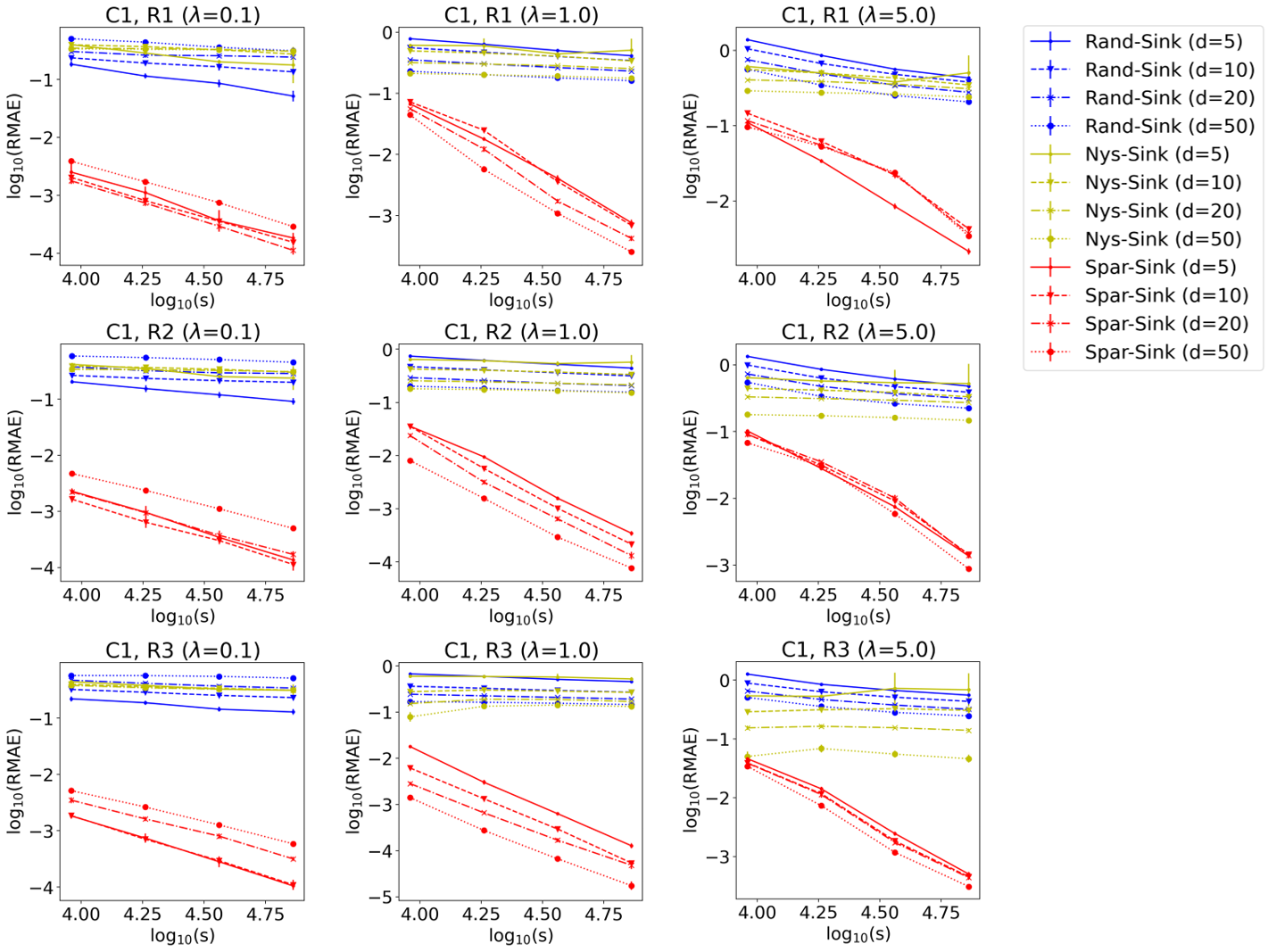
Figure 8: Comparison of subsampling-based methods w.r.t. $\operatorname{RMAE}^{(\operatorname{UOT})}$ versus increasing $s$ (in log-log scale). Each row represents a different sparsity ratio (R1—R3), and each column represents a different $\lambda$. Different methods are marked by different colors, respectively, and each line type represents a different dimension $d$. Vertical bars are the standard errors.

C.2 Asymptotic Convergence

To demonstrate the asymptotic convergence of our proposed method, we display the estimation error $\operatorname{RMAE}^{(\operatorname{OT})}$ versus increasing sample sizes $n$ in Fig. 9, where $n\in\{2^{0},2^{1},\ldots,2^{6}\}\times 10^{2}$, $s=8s_{0}(n)$, and $\varepsilon=0.1$. Other choices of $\varepsilon$ yield similar results and thus are omitted here. In Fig. 9, the Spar-Sink algorithm always yields a smaller estimation error than competitors. Notably, when $d$ is relatively large (e.g., $d\geq 10$), $\operatorname{RMAE}^{(\operatorname{OT})}$ of Spar-Sink decreases substantially faster than that of Nys-Sink, which indicates a higher convergence rate.

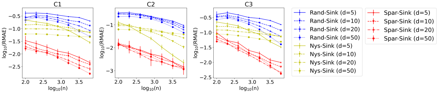
Figure 9: Comparison of different methods w.r.t. $\operatorname{RMAE}^{(\operatorname{OT})}$ versus increasing $n$ (in log-log scale). Each column represents a different data generation pattern (C1—C3). Vertical bars are the standard errors.

Figure 10 displays the results of $\operatorname{RMAE}^{(\operatorname{UOT})}$ versus increasing $n$ and $s=8s_{0}(n)$, under $\varepsilon=0.1$ and $\lambda=0.1$. As shown in Fig. 10, the estimations of both Rand-Sink and Nys-Sink methods become worse as $n$ grows, while Spar-Sink converges significantly faster with the increase of $n$.

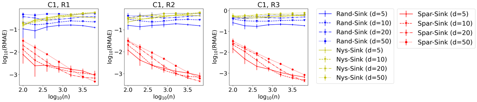
Figure 10: Comparison of different methods w.r.t. $\operatorname{RMAE}^{(\operatorname{UOT})}$ versus increasing $n$ (in log-log scale). Each column represents a different sparsity ratio (R1—R3). Vertical bars are the standard errors.

C.3 Approximation of Wasserstein Barycenters

Experiments on synthetic data. We compare the proposed Spar-IBP method with the classical IBP method, as well as two subsampling-based methods, Nys-IBP and Rand-IBP, which are direct extensions of Nys-Sink and Rand-Sink to approximate Wasserstein barycenters, respectively.

The input probability measures $\bm{b}_{1},\bm{b}_{2},\bm{b}_{3}\in\Delta^{n-1}$ are generated as:

• $\bm{b}_{1}$ is an empirical Gaussian distribution $N(\frac{1}{5},\frac{1}{50})$;

• $\bm{b}_{2}$ is an empirical Gaussian mixture distribution $\frac{1}{2}N(\frac{1}{2},\frac{1}{60})+\frac{1}{2}N(\frac{4}{5},\frac{1}{80})$;

• $\bm{b}_{3}$ is an empirical t-distribution with 5 degrees of freedom $t_{5}(\frac{3}{5},\frac{1}{100})$.

After generating the measures as above, we add $10^{-2}\max_{i\in[n]}b_{k,i}$ to each component of $\bm{b}_{k}$ and then normalize it such that $\sum_{i\in[n]}b_{k,i}=1$, for $k\in[m]$. Suppose the measures and their barycenter share the same support points $\{\bm{x}_{i}\}_{i=1}^{n}$, where $\bm{x}_{i}$’s are randomly and uniformly located over $(0,1)^{d}$, with $n=10^{3}$ and $d\in\{5,10,20\}$. Then, the cost matrices $\mathbf{C}_{1}=\mathbf{C}_{2}=\mathbf{C}_{3}$ are defined by squared Euclidean distances. We set $\bm{w}=\mathbf{1}_{m}/m$, $\varepsilon\in\{5,5^{0},5^{-1}\}\times 10^{-2}$ and $s=\{5,10,15,20\}\times s_{0}(n)$ with $s_{0}(n)=10^{-3}n\log^{4}(n)$. For comparison, we calculate the approximation error of each estimator based on 100 replications, i.e.,

$$\operatorname{Error}=\frac{1}{100}\sum_{i=1}^{100}\|\widetilde{\bm{q}}_{\varepsilon}^{\ast(i)}-\bm{q}_{\varepsilon}^{\ast(i)}\|_{1},$$

where $\widetilde{\bm{q}}_{\varepsilon}^{\ast(i)}$ represents the estimator in the $i$th replication, and $\bm{q}_{\varepsilon}^{\ast(i)}$ is obtained by the IBP algorithm. The results are shown in Fig. 11, from which we observe the proposed Spar-IBP method outperforms competitors in most circumstances, with its advantage becoming more prominent as the value of $\varepsilon$ decreases. The comparison of CPU time has similar pattern to Fig. 5 and is omitted here.

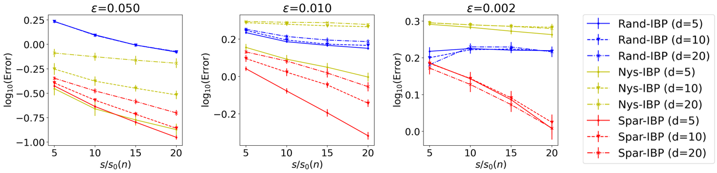
Figure 11: Comparison of different methods w.r.t. $\log_{10}(\operatorname{Error})$ versus increasing $s/s_{0}(n)$ under different levels of $\varepsilon$. Each color marks a specific method, and each line type represents a different dimension $d$. Vertical bars are the standard errors.

Experiments on MNIST. Further, we evaluate our Spar-IBP algorithm on the MNIST data set (LeCun et al., 1998) following the work of Cuturi and Doucet (2014). For each digit from 0 to 9, we randomly select 15 images from the data set, and uniformly rescale each image between half-size and double-size of its original scale at random. After that, each image is normalized such that all pixel values add up to 1. Then, the images are translated randomly within a $64\times 64$ grid, with a bias towards corners. Given the reshaped images with equal weights (i.e., $\bm{w}=\mathbf{1}_{m}/m$), we compute their Wasserstein barycenter. We also include the performance of the IBP algorithm for comparison. The images and results are shown in Fig. 12. The regularization parameter is set to be $\varepsilon=10^{-3}$ for both methods, and the subsample parameter is taken as $s=20s_{0}(n)$ for Spar-IBP.

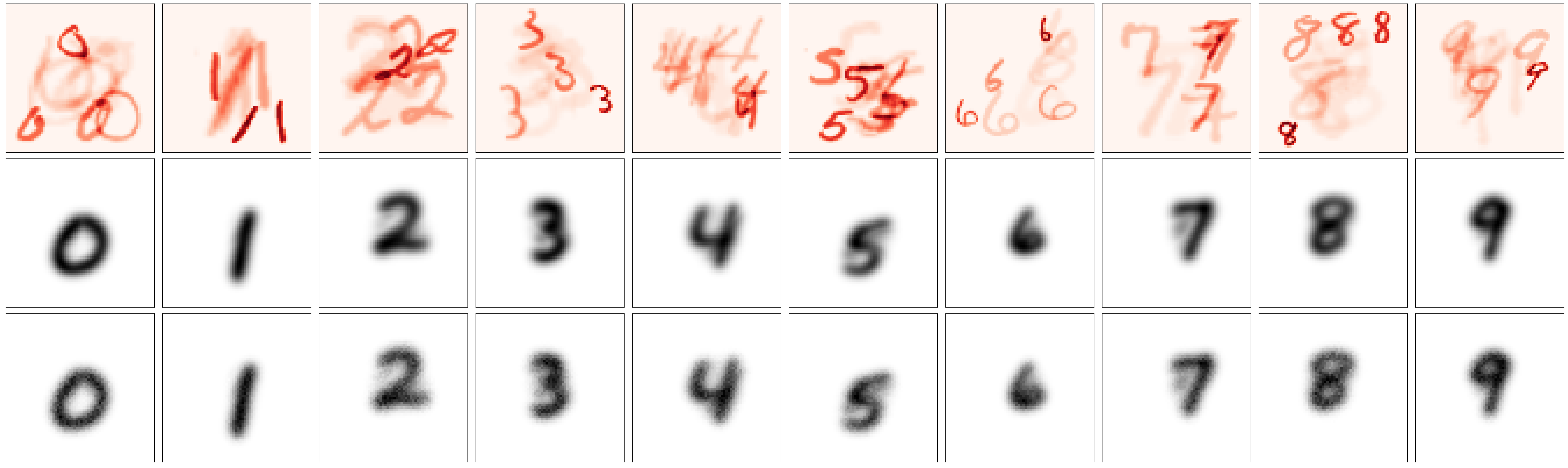
Figure 12: (Top row) For each digit, 8 out of the 15 rescaled and translated images are randomly chosen for illustration. (Middle row) Barycenters approximated by the IBP method. (Bottom row) Barycenters approximated by the Spar-IBP method.

In Fig. 12, we observe the approximate barycenters generated by Spar-IBP are almost as clear as those obtained by IBP. Furthermore, with an average CPU time of 27.50s to compute one barycenter, Spar-IBP is considerably more efficient than IBP, which requires 340.29s. Such results demonstrate the effectiveness and efficiency of our Spar-IBP method for approximating Wasserstein barycenters.

Appendix D Applications

Following the recent work of Le et al. (2021) and Li et al. (2022), we evaluate the performance of our proposed Spar-Sink method in two applications, color transfer and generative modeling.

D.1 Color Transfer

The objective is to transfer the color of an ocean sunset image to an ocean daytime image, as depicted in Fig. 13(a). The pixels of each image can be represented as point clouds in the three-dimensional RGB space. Due to the large number of pixels in each image, which is nearly a million, we follow the preprocessing step in Ferradans et al. (2014) and Le et al. (2021) to randomly downsample $n=5000$ pixels from each image, resulting in $\{\bm{x}_{i}\}_{i=1}^{n},\{\bm{y}_{j}\}_{j=1}^{n}\subset\mathbb{R}^{3}$ and use discrete uniform distributions to define $\bm{a},\bm{b}\in\Delta^{n-1}$. We construct the cost matrix $\mathbf{C}$ using pairwise squared Euclidean distances, that is, $C_{ij}=\|\bm{x}_{i}-\bm{y}_{j}\|_{2}^{2}$. To generate a new image with source content and target color, we compute the optimal transportation plan between $\bm{a}$ and $\bm{b}$ and extend the plan to the entire image using the nearest neighbor interpolation proposed by Ferradans et al. (2014).

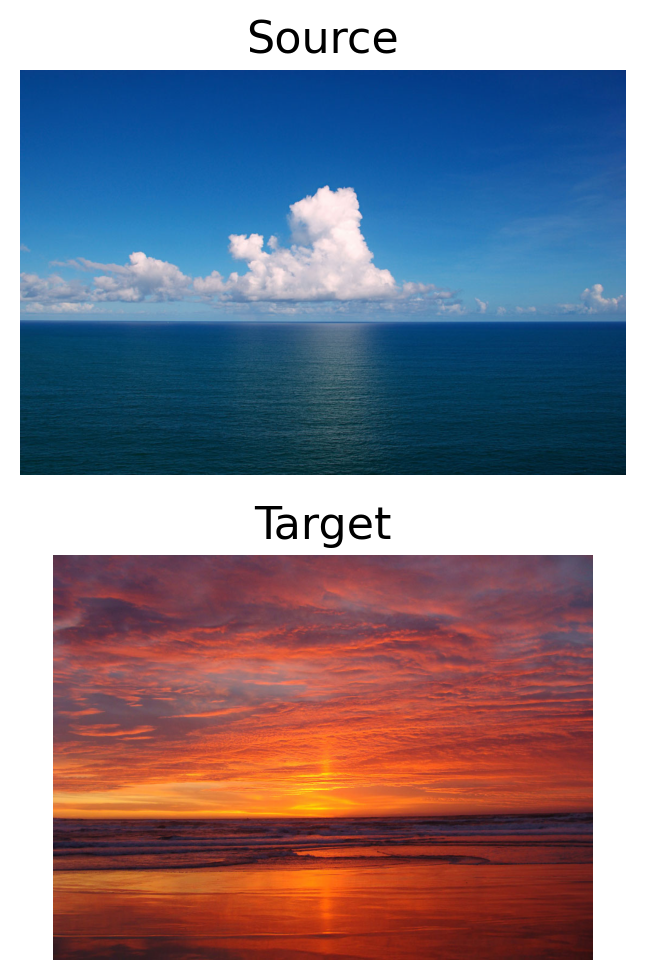
(a) Source and target images.

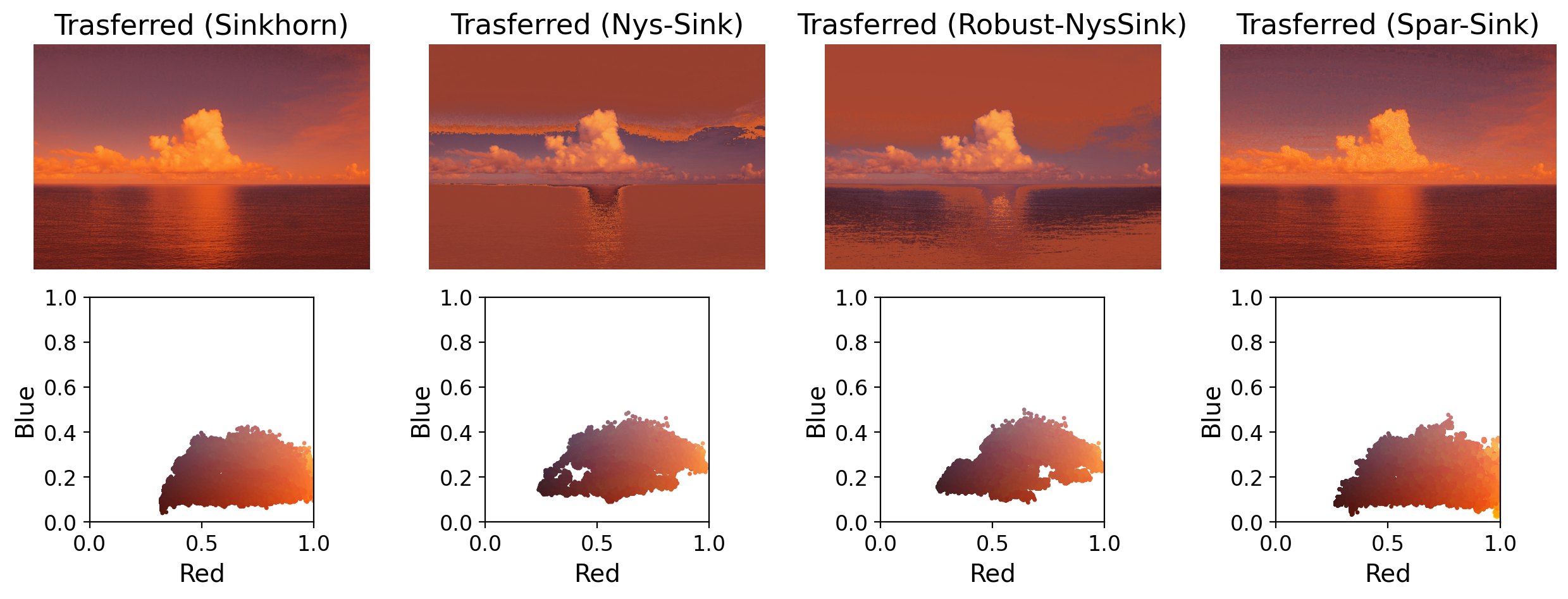
(b) Transferred images with source content and target color, respectively achieved by Sinkhorn, Nys-Sink, Robust-NysSink, and Spar-Sink (ours).

Figure 13: Comparison of different methods on color transfer. Subfigure (b): (Top row) Transferred images. (Bottom row) The corresponding point clouds in RGB space. The color of the dot represents each point’s RGB value.

To approximate the optimal transportation plan, we compare various methods, including the Sinkhorn, Nys-Sink, and Spar-Sink in classical OT formulations, as well as the Robust-NysSink from the robust OT framework (Le et al., 2021). In this experiment, we set $\varepsilon=10^{-2}$ and $\lambda=10$, where $\lambda$ is the marginal regularized parameter in Robust-NysSink. For subsampling-based approaches, we take $s=8s_{0}(n)$ for Spar-Sink, and $r=\lceil s/n\rceil$ for Nys-Sink and Robust-NysSink.

The results of the transferred images generated by these methods are presented in Fig. 13(b). Among the evaluated methods, we observe that Spar-Sink produces a transferred image that closely resembles the result of Sinkhorn, and its corresponding RGB scatter diagram is also similar to that of Sinkhorn. In terms of computational efficiency, the CPU time of computing the plan is 60.45s (Sinkhorn), 12.92s (Nys-Sink), 27.74s (Robust-NysSink), and 3.15s (Spar-Sink), respectively. These results demonstrate the effectiveness of our method on this common computer vision application.

D.2 Generative Modeling

In this section, we introduce a new variant of the Sinkhorn auto-encoder (SAE) (Patrini et al., 2020), named Spar-Sink auto-encoder (SSAE), by using the proposed Spar-Sink approach. Specifically, we employ Spar-Sink to approximate the Sinkhorn divergence (Genevay et al., 2018, 2019; Feydy et al., 2019) between the latent prior distribution and the expected posterior distribution during the training of auto-encoders. We assess the efficacy of this newly proposed generative model in several image generation tasks and compare it with the original SAE.

Assume $f$ (resp. $g$) is an encoder (resp. decoder) parameterized by a neural network, and $p_{Z}$ is a prior distribution on the latent space. Given a set of samples from a data distribution, i.e., $x_{1},\ldots,x_{N}\sim p_{X}$, the objective of SAE is formulated as

$$\min_{f,g}\frac{1}{N}\sum_{i=1}^{N}c\left(x_{i},g(f(x_{i}))\right)+\gamma S\left(f_{\#}p_{X},p_{Z}\right),$$

where $f_{\#}$ denotes the push-forward operator, $c(\cdot,\cdot)$ represents the reconstruction loss, and $S(\cdot,\cdot)$ is a regularizer with weight $\gamma>0$ defined by Sinkhorn divergence, that is,

$$S\left(f_{\#}p_{X},p_{Z}\right)=\operatorname{OT}_{\varepsilon}\left(f_{\#}p_{X},p_{Z}\right)-\frac{1}{2}\left(\operatorname{OT}_{\varepsilon}\left(f_{\#}p_{X},f_{\#}p_{X}\right)+\operatorname{OT}_{\varepsilon}\left(p_{Z},p_{Z}\right)\right).$$ (41)

The objective of SSAE replaces $\operatorname{OT}_{\varepsilon}(\cdot,\cdot)$ in (41) with its approximation, $\widetilde{\operatorname{OT}}_{\varepsilon}(\cdot,\cdot)$, computed using Algorithm 3.

We train auto-encoders to embed the MNIST data (LeCun et al., 1998) into a 10-dimensional latent space. The auto-encoding architecture is identical to that used in Kolouri et al. (2019). We use the Euclidean distance as the distance between samples, the binary cross entropy plus $\ell_{1}$ loss as the reconstruction loss, the standard Gaussian distribution as $p_{Z}$, and Adam (Kingma and Ba, 2014) as the optimizer. For fairness, both SAE and SSAE employ the same hyperparameters: the regularization parameters are $\gamma=0.05$ and $\varepsilon=0.01$; the number of epochs is 40; the batch size $n=500$; the learning rate is $0.001$; other parameters are set by default. Additionally, we set the subsample parameter $s=10s_{0}(n)$ for SSAE.

We compare SAE and SSAE w.r.t. Fréchet inception distance (FID) (Heusel et al., 2017) between $10,000$ test samples and $10,000$ randomly generated samples, and also record their running time on an RTX 3090 GPU. The comparison is conducted based on 100 replications, and the results are presented in Table 2, which shows that the proposed SSAE generator achieves a smaller FID in just half the time compared to SAE. Moreover, we provide image interpolation and reconstruction results obtained by SSAE in Fig. 14, further highlighting the capability of our proposed method in generative modeling tasks.

Methods	FID	Time
SAE	24.72±0.13	125.87
SSAE	23.65±0.06	64.81

Table 2: Comparisons on learning image generators w.r.t. average FID score (with standard deviations presented in footnotes) and running time (in seconds) of an epoch iteration.

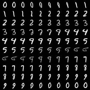
(a) Digit interpolation.

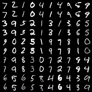
(b) Digit reconstruction.

Figure 14: The performance of SSAE on digit interpolation and reconstruction tasks. In the subfigure (b), odd rows correspond to real images.

References

- Achlioptas and Mcsherry (2007) Dimitris Achlioptas and Frank Mcsherry. Fast computation of low-rank matrix approximations. Journal of the Association for Computing Machinery, 54(2):1–19, 2007.
- Achlioptas et al. (2013) Dimitris Achlioptas, Zohar S Karnin, and Edo Liberty. Near-optimal entrywise sampling for data matrices. Advances in Neural Information Processing Systems, 26:1565–1573, 2013.
- Agueh and Carlier (2011) Martial Agueh and Guillaume Carlier. Barycenters in the Wasserstein space. SIAM Journal on Mathematical Analysis, 43(2):904–924, 2011.
- Alaya et al. (2019) Mokhtar Z Alaya, Maxime Berar, Gilles Gasso, and Alain Rakotomamonjy. Screening Sinkhorn algorithm for regularized optimal transport. Advances in Neural Information Processing Systems, 32:12169–12179, 2019.
- Altschuler et al. (2017) Jason Altschuler, Jonathan Weed, and Philippe Rigollet. Near-linear time approximation algorithms for optimal transport via Sinkhorn iteration. Advances in Neural Information Processing Systems, 30:1961–1971, 2017.
- Altschuler et al. (2019) Jason Altschuler, Francis Bach, Alessandro Rudi, and Jonathan Niles-Weed. Massively scalable Sinkhorn distances via the Nyström method. Advances in Neural Information Processing Systems, 32:4427–4437, 2019.
- An et al. (2022) Dongsheng An, Na Lei, Xiaoyin Xu, and Xianfeng Gu. Efficient optimal transport algorithm by accelerated gradient descent. In Proceedings of the AAAI Conference on Artificial Intelligence, volume 36, pages 10119–10128. AAAI, 2022.
- Arjovsky et al. (2017) Martin Arjovsky, Soumith Chintala, and Léon Bottou. Wasserstein generative adversarial networks. In International Conference on Machine Learning, volume 70, pages 214–223. PMLR, 2017.
- Arora et al. (2006) Sanjeev Arora, Elad Hazan, and Satyen Kale. A fast random sampling algorithm for sparsifying matrices. In Approximation, Randomization, and Combinatorial Optimization. Algorithms and Techniques, pages 272–279. Springer, 2006.
- Balaji et al. (2020) Yogesh Balaji, Rama Chellappa, and Soheil Feizi. Robust optimal transport with applications in generative modeling and domain adaptation. Advances in Neural Information Processing Systems, 33:12934–12944, 2020.
- Benamou et al. (2002) J-D Benamou, Yann Brenier, and Kevin Guittet. The Monge–Kantorovitch mass transfer and its computational fluid mechanics formulation. International Journal for Numerical Methods in Fluids, 40(1-2):21–30, 2002.
- Benamou et al. (2015) Jean-David Benamou, Guillaume Carlier, Marco Cuturi, Luca Nenna, and Gabriel Peyré. Iterative Bregman projections for regularized transportation problems. SIAM Journal on Scientific Computing, 37(2):A1111–A1138, 2015.
- Bonneel et al. (2015) Nicolas Bonneel, Julien Rabin, Gabriel Peyré, and Hanspeter Pfister. Sliced and Radon Wasserstein barycenters of measures. Journal of Mathematical Imaging and Vision, 51(1):22–45, 2015.
- Bouhlel et al. (2020) Imen Bouhlel, Imen Chabchoub, Emna Hajri, Samia Ernez, and Jeridi Gouider. Early screening of cardiotoxicity of chemotherapy by echocardiography and myocardial biomarkers. La Tunisie Medicale, 98(12):1017–1023, 2020.
- Boureau et al. (2010) Y-Lan Boureau, Francis Bach, Yann LeCun, and Jean Ponce. Learning mid-level features for recognition. In 2010 IEEE Computer Society Conference on Computer Vision and Pattern Recognition, pages 2559–2566. IEEE, 2010.
- Braverman et al. (2021) Vladimir Braverman, Robert Krauthgamer, Aditya R Krishnan, and Shay Sapir. Near-optimal entrywise sampling of numerically sparse matrices. In Proceedings of Thirty-Fourth Conference on Learning Theory, volume 134, pages 759–773. PMLR, 2021.
- Brenier (1997) Yann Brenier. A homogenized model for vortex sheets. Archive for Rational Mechanics and Analysis, 138(4):319–353, 1997.
- Candès and Tao (2010) Emmanuel J Candès and Terence Tao. The power of convex relaxation: Near-optimal matrix completion. IEEE Transactions on Information Theory, 56(5):2053–2080, 2010.
- Chen et al. (2014) Yudong Chen, Srinadh Bhojanapalli, Sujay Sanghavi, and Rachel Ward. Coherent matrix completion. In International Conference on Machine Learning, pages 674–682. PMLR, 2014.
- Chizat et al. (2018a) Lenaic Chizat, Gabriel Peyré, Bernhard Schmitzer, and François-Xavier Vialard. An interpolating distance between optimal transport and Fisher–Rao metrics. Foundations of Computational Mathematics, 18(1):1–44, 2018a.
- Chizat et al. (2018b) Lenaic Chizat, Gabriel Peyré, Bernhard Schmitzer, and François-Xavier Vialard. Scaling algorithms for unbalanced optimal transport problems. Mathematics of Computation, 87(314):2563–2609, 2018b.
- Chizat et al. (2018c) Lenaic Chizat, Gabriel Peyré, Bernhard Schmitzer, and François-Xavier Vialard. Unbalanced optimal transport: Dynamic and Kantorovich formulations. Journal of Functional Analysis, 274(11):3090–3123, 2018c.
- Courty et al. (2016) Nicolas Courty, Rémi Flamary, Devis Tuia, and Alain Rakotomamonjy. Optimal transport for domain adaptation. IEEE Transactions on Pattern Analysis and Machine Intelligence, 39(9):1853–1865, 2016.
- Cuturi (2013) Marco Cuturi. Sinkhorn distances: Lightspeed computation of optimal transport. Advances in Neural Information Processing Systems, 26:2292–2300, 2013.
- Cuturi and Doucet (2014) Marco Cuturi and Arnaud Doucet. Fast computation of Wasserstein barycenters. In International Conference on Machine Learning, volume 32, pages 685–693. PMLR, 2014.
- Cuturi and Peyré (2018) Marco Cuturi and Gabriel Peyré. Semidual regularized optimal transport. SIAM Review, 60(4):941–965, 2018.
- Deshpande et al. (2019) Ishan Deshpande, Yuan-Ting Hu, Ruoyu Sun, Ayis Pyrros, Nasir Siddiqui, Sanmi Koyejo, Zhizhen Zhao, David Forsyth, and Alexander G Schwing. Max-sliced Wasserstein distance and its use for GANs. In Proceedings of the IEEE/CVF Conference on Computer Vision and Pattern Recognition, pages 10648–10656. IEEE, 2019.
- Drineas and Zouzias (2011) Petros Drineas and Anastasios Zouzias. A note on element-wise matrix sparsification via a matrix-valued Bernstein inequality. Information Processing Letters, 111(8):385–389, 2011.
- Drineas et al. (2006) Petros Drineas, Ravi Kannan, and Michael W Mahoney. Fast Monte Carlo algorithms for matrices I: Approximating matrix multiplication. SIAM Journal on Computing, 36(1):132–157, 2006.
- Dubey and Müller (2020) Paromita Dubey and Hans-Georg Müller. Functional models for time-varying random objects. Journal of the Royal Statistical Society: Series B (Statistical Methodology), 82(2):275–327, 2020.
- Ferradans et al. (2014) Sira Ferradans, Nicolas Papadakis, Gabriel Peyré, and Jean-François Aujol. Regularized discrete optimal transport. SIAM Journal on Imaging Sciences, 7(3):1853–1882, 2014.
- Feydy et al. (2019) Jean Feydy, Thibault Séjourné, François-Xavier Vialard, Shun-ichi Amari, Alain Trouvé, and Gabriel Peyré. Interpolating between optimal transport and MMD using Sinkhorn divergences. In International Conference on Artificial Intelligence and Statistics, volume 89, pages 2681–2690. PMLR, 2019.
- Flamary et al. (2018) Rémi Flamary, Marco Cuturi, Nicolas Courty, and Alain Rakotomamonjy. Wasserstein discriminant analysis. Machine Learning, 107(12):1923–1945, 2018.
- Flamary et al. (2021) Rémi Flamary, Nicolas Courty, Alexandre Gramfort, Mokhtar Z. Alaya, Aurélie Boisbunon, Stanislas Chambon, Laetitia Chapel, Adrien Corenflos, Kilian Fatras, Nemo Fournier, Léo Gautheron, Nathalie T.H. Gayraud, Hicham Janati, Alain Rakotomamonjy, Ievgen Redko, Antoine Rolet, Antony Schutz, Vivien Seguy, Danica J. Sutherland, Romain Tavenard, Alexander Tong, and Titouan Vayer. POT: Python optimal transport. The Journal of Machine Learning Research, 22(1):3571–3578, 2021.
- Frogner et al. (2015) Charlie Frogner, Chiyuan Zhang, Hossein Mobahi, Mauricio Araya, and Tomaso A Poggio. Learning with a Wasserstein loss. Advances in Neural Information Processing Systems, 28:2053–2061, 2015.
- Fye (2015) W Bruce Fye. Caring for the heart: Mayo Clinic and the rise of specialization. Oxford University Press, 2015.
- Genevay et al. (2018) Aude Genevay, Gabriel Peyré, and Marco Cuturi. Learning generative models with Sinkhorn divergences. In International Conference on Artificial Intelligence and Statistics, volume 84, pages 1608–1617. PMLR, 2018.
- Genevay et al. (2019) Aude Genevay, Lénaic Chizat, Francis Bach, Marco Cuturi, and Gabriel Peyré. Sample complexity of Sinkhorn divergences. In International Conference on Artificial Intelligence and Statistics, volume 89, pages 1574–1583. PMLR, 2019.
- Gong et al. (2014) Yunchao Gong, Liwei Wang, Ruiqi Guo, and Svetlana Lazebnik. Multi-scale orderless pooling of deep convolutional activation features. In European Conference on Computer Vision, pages 392–407. Springer, 2014.
- Guminov et al. (2021) Sergey Guminov, Pavel Dvurechensky, Nazarii Tupitsa, and Alexander Gasnikov. On a combination of alternating minimization and Nesterov’s momentum. In International Conference on Machine Learning, volume 139, pages 3886–3898. PMLR, 2021.
- Guo et al. (2020) Wenshuo Guo, Nhat Ho, and Michael I Jordan. Fast algorithms for computational optimal transport and Wasserstein barycenter. In International Conference on Artificial Intelligence and Statistics, volume 108, pages 2088–2097. PMLR, 2020.
- Gupta and Sidford (2018) Neha Gupta and Aaron Sidford. Exploiting numerical sparsity for efficient learning: Faster eigenvector computation and regression. Advances in Neural Information Processing Systems, 31:5274–5283, 2018.
- Heusel et al. (2017) Martin Heusel, Hubert Ramsauer, Thomas Unterthiner, Bernhard Nessler, and Sepp Hochreiter. GANs trained by a two time-scale update rule converge to a local Nash equilibrium. Advances in Neural Information Processing Systems, 30, 2017.
- Kahn and Marshall (1953) Herman Kahn and Andy W Marshall. Methods of reducing sample size in Monte Carlo computations. Journal of the Operations Research Society of America, 1(5):263–278, 1953.
- Kantorovich (1942) L Kantorovich. On the transfer of masses (in Russian). In Doklady Akademii Nauk, volume 37, pages 227–229, 1942.
- Katharopoulos and Fleuret (2018) Angelos Katharopoulos and François Fleuret. Not all samples are created equal: Deep learning with importance sampling. In International Conference on Machine Learning, volume 80, pages 2525–2534. PMLR, 2018.
- Kingma and Ba (2014) Diederik P Kingma and Jimmy Ba. Adam: A method for stochastic optimization. arXiv preprint arXiv:1412.6980, 2014.
- Klicpera et al. (2021) Johannes Klicpera, Marten Lienen, and Stephan Günnemann. Scalable optimal transport in high dimensions for graph distances, embedding alignment, and more. In International Conference on Machine Learning, volume 139, pages 5616–5627. PMLR, 2021.
- Kolouri et al. (2019) Soheil Kolouri, Phillip E Pope, Charles E Martin, and Gustavo K Rohde. Sliced Wasserstein auto-encoders. In International Conference on Learning Representations, 2019.
- Kondratyev et al. (2016) Stanislav Kondratyev, Léonard Monsaingeon, and Dmitry Vorotnikov. A new optimal transport distance on the space of finite Radon measures. Advances in Differential Equations, 21(11/12):1117–1164, 2016.
- Kroshnin et al. (2019) Alexey Kroshnin, Nazarii Tupitsa, Darina Dvinskikh, Pavel Dvurechensky, Alexander Gasnikov, and Cesar Uribe. On the complexity of approximating Wasserstein barycenters. In International Conference on Machine Learning, volume 97, pages 3530–3540. PMLR, 2019.
- Kumar et al. (2012) Sanjiv Kumar, Mehryar Mohri, and Ameet Talwalkar. Sampling methods for the Nyström method. The Journal of Machine Learning Research, 13(1):981–1006, 2012.
- Kundu et al. (2017) Abhisek Kundu, Petros Drineas, and Malik Magdon-Ismail. Recovering PCA and sparse PCA via hybrid- sparse sampling of data elements. The Journal of Machine Learning Research, 18(1):2558–2591, 2017.
- Le et al. (2021) Khang Le, Huy Nguyen, Quang M Nguyen, Tung Pham, Hung Bui, and Nhat Ho. On robust optimal transport: Computational complexity and barycenter computation. Advances in Neural Information Processing Systems, 34:21947–21959, 2021.
- LeCun et al. (1998) Yann LeCun, Léon Bottou, Yoshua Bengio, and Patrick Haffner. Gradient-based learning applied to document recognition. Proceedings of the IEEE, 86(11):2278–2324, 1998.
- Lee and Sidford (2014) Yin Tat Lee and Aaron Sidford. Path finding methods for linear programming: Solving linear programs in (vrank) iterations and faster algorithms for maximum flow. In IEEE 55th Annual Symposium on Foundations of Computer Science, pages 424–433. IEEE, 2014.
- Lee and Sidford (2015) Yin Tat Lee and Aaron Sidford. Efficient inverse maintenance and faster algorithms for linear programming. In IEEE 56th Annual Symposium on Foundations of Computer Science, pages 230–249. IEEE, 2015.
- Li et al. (2023) Mengyu Li, Jun Yu, Hongteng Xu, and Cheng Meng. Efficient approximation of Gromov-Wasserstein distance using importance sparsification. Journal of Computational and Graphical Statistics, pages 1–25, 2023.
- Li et al. (2022) Tao Li, Cheng Meng, Jun Yu, and Hongteng Xu. Hilbert curve projection distance for distribution comparison. arXiv preprint arXiv:2205.15059, 2022.
- Liao et al. (2022a) Qichen Liao, Jing Chen, Zihao Wang, Bo Bai, Shi Jin, and Hao Wu. Fast Sinkhorn I: An algorithm for the Wasserstein-1 metric. arXiv preprint arXiv:2202.10042, 2022a.
- Liao et al. (2022b) Qichen Liao, Zihao Wang, Jing Chen, Bo Bai, Shi Jin, and Hao Wu. Fast Sinkhorn II: Collinear triangular matrix and linear time accurate computation of optimal transport. arXiv preprint arXiv:2206.09049, 2022b.
- Liero et al. (2016) Matthias Liero, Alexander Mielke, and Giuseppe Savaré. Optimal transport in competition with reaction: The Hellinger–Kantorovich distance and geodesic curves. SIAM Journal on Mathematical Analysis, 48(4):2869–2911, 2016.
- Liero et al. (2018) Matthias Liero, Alexander Mielke, and Giuseppe Savaré. Optimal entropy-transport problems and a new Hellinger–Kantorovich distance between positive measures. Inventiones Mathematicae, 211(3):969–1117, 2018.
- Lin et al. (2019a) Tianyi Lin, Nhat Ho, and Michael I Jordan. On the acceleration of the Sinkhorn and Greenkhorn algorithms for optimal transport. arXiv preprint arXiv:1906.01437, 2019a.
- Lin et al. (2019b) Tianyi Lin, Nhat Ho, and Michael I Jordan. On efficient optimal transport: An analysis of greedy and accelerated mirror descent algorithms. In International Conference on Machine Learning, volume 97, pages 3982–3991. PMLR, 2019b.
- Lin et al. (2020) Tianyi Lin, Nhat Ho, Xi Chen, Marco Cuturi, and Michael Jordan. Fixed-support Wasserstein barycenters: Computational hardness and fast algorithm. Advances in Neural Information Processing Systems, 33:5368–5380, 2020.
- Lin et al. (2022) Tianyi Lin, Nhat Ho, and Michael I Jordan. On the efficiency of entropic regularized algorithms for optimal transport. The Journal of Machine Learning Research, 23(137):1–42, 2022.
- Liu (1996) Jun S Liu. Metropolized independent sampling with comparisons to rejection sampling and importance sampling. Statistics and Computing, 6(2):113–119, 1996.
- Liu (2008) Jun S Liu. Monte Carlo Strategies in Scientific Computing. Springer, 2008.
- Ma et al. (2015) Ping Ma, Michael W Mahoney, and Bin Yu. A statistical perspective on algorithmic leveraging. The Journal of Machine Learning Research, 16(1):861–911, 2015.
- Mahoney (2011) Michael W Mahoney. Randomized algorithms for matrices and data. Foundations and Trends® in Machine Learning, 3(2):123–224, 2011.
- Marouf et al. (2020) Mohamed Marouf, Pierre Machart, Vikas Bansal, Christoph Kilian, Daniel S Magruder, Christian F Krebs, and Stefan Bonn. Realistic in silico generation and augmentation of single-cell RNA-seq data using generative adversarial networks. Nature Communications, 11(1):1–12, 2020.
- Meng et al. (2019) Cheng Meng, Yuan Ke, Jingyi Zhang, Mengrui Zhang, Wenxuan Zhong, and Ping Ma. Large-scale optimal transport map estimation using projection pursuit. Advances in Neural Information Processing Systems, 32:8118–8129, 2019.
- Meng et al. (2020) Cheng Meng, Jun Yu, Jingyi Zhang, Ping Ma, and Wenxuan Zhong. Sufficient dimension reduction for classification using principal optimal transport direction. Advances in Neural Information Processing Systems, 33:4015–4028, 2020.
- Montavon et al. (2016) Grégoire Montavon, Klaus-Robert Müller, and Marco Cuturi. Wasserstein training of restricted Boltzmann machines. Advances in Neural Information Processing Systems, 29:3718–3726, 2016.
- Montesuma and Mboula (2021) Eduardo Fernandes Montesuma and Fred Maurice Ngole Mboula. Wasserstein barycenter for multi-source domain adaptation. In Proceedings of the IEEE/CVF Conference on Computer Vision and Pattern Recognition, pages 16785–16793, 2021.
- Muzellec et al. (2020) Boris Muzellec, Julie Josse, Claire Boyer, and Marco Cuturi. Missing data imputation using optimal transport. In International Conference on Machine Learning, volume 119, pages 7130–7140. PMLR, 2020.
- Nadjahi (2021) Kimia Nadjahi. Sliced-Wasserstein distance for large-scale machine learning: Theory, methodology and extensions. PhD thesis, Institut polytechnique de Paris, 2021.
- Nguyen et al. (2021) Khai Nguyen, Nhat Ho, Tung Pham, and Hung Bui. Distributional sliced-Wasserstein and applications to generative modeling. In International Conference on Learning Representations, 2021.
- Nguyen et al. (2023) Khai Nguyen, Tongzheng Ren, Huy Nguyen, Litu Rout, Tan Nguyen, and Nhat Ho. Hierarchical sliced Wasserstein distance. In International Conference on Learning Representations, 2023.
- Ouyang et al. (2020) David Ouyang, Bryan He, Amirata Ghorbani, Neal Yuan, Joseph Ebinger, Curtis P Langlotz, Paul A Heidenreich, Robert A Harrington, David H Liang, Euan A Ashley, and James Y Zou. Video-based AI for beat-to-beat assessment of cardiac function. Nature, 580(7802):252–256, 2020.
- Owen (2013) Art B Owen. Monte Carlo Theory, Methods and Examples. 2013.
- Panaretos and Zemel (2019) Victor M Panaretos and Yoav Zemel. Statistical aspects of Wasserstein distances. Annual Review of Statistics and Its Application, 6(1):405–431, 2019.
- Patrini et al. (2020) Giorgio Patrini, Rianne van den Berg, Patrick Forré, Marcello Carioni, Samarth Bhargav, Max Welling, Tim Genewein, and Frank Nielsen. Sinkhorn autoencoders. In Proceedings of The 35th Uncertainty in Artificial Intelligence Conference, volume 115, pages 733–743. PMLR, 2020.
- Pele and Werman (2009) Ofir Pele and Michael Werman. Fast and robust earth mover’s distances. In IEEE 12th International Conference on Computer Vision, pages 460–467. IEEE, 2009.
- Peyré and Cuturi (2019) Gabriel Peyré and Marco Cuturi. Computational optimal transport: With applications to data science. Foundations and Trends® in Machine Learning, 11(5-6):355–607, 2019.
- Pham et al. (2020) Khiem Pham, Khang Le, Nhat Ho, Tung Pham, and Hung Bui. On unbalanced optimal transport: An analysis of Sinkhorn algorithm. In International Conference on Machine Learning, volume 119, pages 7673–7682. PMLR, 2020.
- Pitié et al. (2005) François Pitié, Anil C Kokaram, and Rozenn Dahyot. N-dimensional probability density function transfer and its application to color transfer. In Tenth IEEE International Conference on Computer Vision, volume 2, pages 1434–1439. IEEE, 2005.
- Rabin et al. (2011) Julien Rabin, Gabriel Peyré, Julie Delon, and Marc Bernot. Wasserstein barycenter and its application to texture mixing. In International Conference on Scale Space and Variational Methods in Computer Vision, volume 6667, pages 435–446. Springer, 2011.
- Rigollet and Weed (2018) Philippe Rigollet and Jonathan Weed. Entropic optimal transport is maximum-likelihood deconvolution. Comptes Rendus Mathematique, 356(11-12):1228–1235, 2018.
- Rubner et al. (1997) Yossi Rubner, Leonidas J Guibas, and Carlo Tomasi. The earth mover’s distance, multi-dimensional scaling, and color-based image retrieval. In Proceedings of the ARPA Image Understanding Workshop, volume 661, page 668. ARPA, 1997.
- Scetbon and Cuturi (2020) Meyer Scetbon and Marco Cuturi. Linear time Sinkhorn divergences using positive features. Advances in Neural Information Processing Systems, 33:13468–13480, 2020.
- Scetbon et al. (2021) Meyer Scetbon, Marco Cuturi, and Gabriel Peyré. Low-rank Sinkhorn factorization. In International Conference on Machine Learning, volume 139, pages 9344–9354. PMLR, 2021.
- Schiebinger et al. (2019) Geoffrey Schiebinger, Jian Shu, Marcin Tabaka, Brian Cleary, Vidya Subramanian, Aryeh Solomon, Joshua Gould, Siyan Liu, Stacie Lin, Peter Berube, Lia Lee, Jenny Chen, Justin Brumbaugh, Philippe Rigollet, Konrad Hochedlinger, Rudolf Jaenisch, Aviv Regev, and Eric S. Lander. Optimal-transport analysis of single-cell gene expression identifies developmental trajectories in reprogramming. Cell, 176(4):928–943, 2019.
- Séjourné et al. (2022) Thibault Séjourné, François-Xavier Vialard, and Gabriel Peyré. Faster unbalanced optimal transport: Translation invariant Sinkhorn and 1-d Frank–Wolfe. In International Conference on Artificial Intelligence and Statistics, pages 4995–5021. PMLR, 2022.
- Sinkhorn and Knopp (1967) Richard Sinkhorn and Paul Knopp. Concerning nonnegative matrices and doubly stochastic matrices. Pacific Journal of Mathematics, 21(2):343–348, 1967.
- Solomon et al. (2015) Justin Solomon, Fernando De Goes, Gabriel Peyré, Marco Cuturi, Adrian Butscher, Andy Nguyen, Tao Du, and Leonidas Guibas. Convolutional Wasserstein distances: Efficient optimal transportation on geometric domains. ACM Transactions on Graphics, 34(4):1–11, 2015.
- Su et al. (2015) Zhengyu Su, Yalin Wang, Rui Shi, Wei Zeng, Jian Sun, Feng Luo, and Xianfeng Gu. Optimal mass transport for shape matching and comparison. IEEE Transactions on Pattern Analysis and Machine Intelligence, 37(11):2246–2259, 2015.
- Tanay and Regev (2017) Amos Tanay and Aviv Regev. Scaling single-cell genomics from phenomenology to mechanism. Nature, 541(7637):331–338, 2017.
- Wang and Zou (2021) HaiYing Wang and Jiahui Zou. A comparative study on sampling with replacement vs Poisson sampling in optimal subsampling. In International Conference on Artificial Intelligence and Statistics, volume 130, pages 289–297. PMLR, 2021.
- Wang et al. (2020) Zihao Wang, Datong Zhou, Ming Yang, Yong Zhang, Chenglong Rao, and Hao Wu. Robust document distance with Wasserstein-Fisher-Rao metric. In Proceedings of the 12th Asian Conference on Machine Learning, volume 129, pages 721–736. PMLR, 2020.
- Xie et al. (2020) Yujia Xie, Xiangfeng Wang, Ruijia Wang, and Hongyuan Zha. A fast proximal point method for computing exact Wasserstein distance. In Proceedings of The 35th Uncertainty in Artificial Intelligence Conference, volume 115, pages 433–453. PMLR, 2020.
- Xu and Cheng (2022) Hongteng Xu and Minjie Cheng. Regularized optimal transport layers for generalized global pooling operations. arXiv preprint arXiv:2212.06339, 2022.
- Xu et al. (2019) Lin Xu, Han Sun, and Yuai Liu. Learning with batch-wise optimal transport loss for 3D shape recognition. In Proceedings of the IEEE/CVF Conference on Computer Vision and Pattern Recognition, pages 3333–3342. IEEE, 2019.
- Yu et al. (2022) Jun Yu, HaiYing Wang, Mingyao Ai, and Huiming Zhang. Optimal distributed subsampling for maximum quasi-likelihood estimators with massive data. Journal of the American Statistical Association, 117(537):265–276, 2022.
- Zhang et al. (2021a) Jingyi Zhang, Wenxuan Zhong, and Ping Ma. A review on modern computational optimal transport methods with applications in biomedical research. Modern Statistical Methods for Health Research, pages 279–300, 2021a.
- Zhang et al. (2021b) Jingyi Zhang, Huolan Zhu, Yongkai Chen, Chenguang Yang, Huimin Cheng, Yi Li, Wenxuan Zhong, and Fang Wang. Ensemble machine learning approach for screening of coronary heart disease based on echocardiography and risk factors. BMC Medical Informatics and Decision Making, 21(1):1–13, 2021b.
- Zhao and Zhang (2015) Peilin Zhao and Tong Zhang. Stochastic optimization with importance sampling for regularized loss minimization. In International Conference on Machine Learning, volume 37, pages 1–9. PMLR, 2015.
- Zhou et al. (2018) DT Zhou, Jing Chen, H Wu, DH Yang, and LY Qiu. The Wasserstein-Fisher-Rao metric for waveform based earthquake location. arXiv preprint arXiv:1812.00304, 2018.