Learning Robust and Consistent Time Series Representations: A Dilated Inception-Based Approach

Abstract

Representation learning for time series has been an important research area for decades. Since the emergence of the foundation models, this topic has attracted a lot of attention in contrastive self-supervised learning, to solve a wide range of downstream tasks. However, there have been several challenges for contrastive time series processing. First, there is no work considering noise, which is one of the critical factors affecting the efficacy of time series tasks. Second, there is a lack of efficient yet lightweight encoder architectures that can learn informative representations robust to various downstream tasks. To fill in these gaps, we initiate a novel sampling strategy that promotes consistent representation learning with the presence of noise in natural time series. In addition, we propose an encoder architecture that utilizes dilated convolution within the Inception block to create a scalable and robust network architecture with a wide receptive field. Experiments demonstrate that our method consistently outperforms state-of-the-art methods in forecasting, classification, and abnormality detection tasks, e.g. ranks first over two-thirds of the classification UCR datasets, with only $40\%$ of the parameters compared to the second-best approach. Our source code for CoInception framework is accessible at https://github.com/anhduy0911/CoInception.

1 Introduction

Motivation. Time series data are prevalent in various fields, including finance, medicine, and engineering, making their analysis crucial in practical applications [45, 49, 42, 4]. However, as time series data usually possess complex pattern that is unrecognizable by humans, obtaining their labels is often challenging and expensive, particularly in domains where data privacy is a priority, such as healthcare and finance [24, 36, 53]. Unsupervised learning offers a potential solution to overcome this obstacle by enabling the ability to learn informative representations that can be utilized in diverse downstream tasks. Unsupervised representation learning has been well-studied in the domains of computer vision and natural language processing [6, 67, 41, 35, 23, 60], but has been under-explored in the literature of time series domain. Recognizing the significance of the task and the existing gaps in current literature [18, 55, 17, 64, 65], this study dedicates to addressing the time series representation learning problem.

We argue that a time series representation learning framework should simultaneously meet the following two criteria: (1) efficiency (i.e., the learned representation should capture essential characteristics of the input time series, providing high accuracy for downstream tasks) and (2) scalability (i.e., the framework should be lightweight as time series data collected in practice can be long, high dimensional, and high frequency).

Related literature and our approach. Prior research on representation learning in time series data has predominantly focused on employing the self-supervised contrastive learning technique [18, 55, 17, 64, 65], which consists of two main components: sampling strategy and encoder architecture.

The existing sampling strategies mainly center around the time series’ invariance characteristics, such as temporal invariance [26, 55, 18], transformation and augmentation invariance [54, 64, 68], and contextual invariance [17, 65]. For example, TNC [55] analyzes stationary properties for sampling positive pairs based on the temporal invariance, but its quadratic complexity limits real-time applicability. BTSF [64] employs instance-level dropout and combines temporal and spectral representations, but its efficiency depends on dropout rate and time instance length. Some studies, such as [17, 65], aim to maintain the contextual invariance of time series data. The work in [65] focuses on maintaining instance-level representations when placed in different contexts (i.e., different time segments). Although this approach has demonstrated the potential of learning contextual-invariant representations, the framework is vulnerable to noise and the lack of interpretability when dealing with alternating noise signals. In addition, note that one of the most prominent distinctions of time series against other data types (e.g., images and texts) is that the real-world time series usually contains much noise, which hampers the accuracy of time series tasks severely [50, 62]. With this realization, we take a unique approach by designing a noise-resistant sampling strategy that captures the underlying structural characteristics of time series, specifically contextual invariance. Our method involves leveraging a low-pass filter to generate correlated yet distinct views of each raw input time series. We then use these augmented views to create positive and negative pairs, effectively modeling the temporal and contextual invariance of time series. The benefits of using low-pass filter-based augmented views are twofold: firstly, the filter preserves essential characteristics like trend and seasonality, ensuring deterministic and interpretable representations; secondly, it removes noise-prone high-frequency components, improving noise resilience and enhancing downstream task performance by aligning the raw signal representation with the augmented view.

While researchers have much interest in developing effective sampling strategies, designing robust frameworks capable of generating representations suitable for various time series tasks is also very important. One common approach involves the use of auto-encoders [10] or sequence-to-sequence models [19, 33]. Other studies have utilized Convolution-based architectures (e.g. Causal Convolution [3, 59, 18] or Dilated Convolution [18, 65]). However, these approaches have limitations in capturing long-term dependencies and may not be suitable for long time series data. Alternatively, versatile Transformer-based architectures and their variants [25, 30, 69] are utilized in addressing the need to capture long-term dependencies in time series analysis. However, these architectures may suffer from computational and resource-intensive requirements. Additionally, notable findings indicate the collapse of Transformer architectures when applied to specific tasks or data [16, 46, 51]. In light of these challenges, our work aims to propose a more efficient and scalable encoder framework to mitigate the limitations observed in previous studies. Our main idea is to leverage the benefits of the Inception architecture and dilated convolution network. In particular, while the Inception framework, with the use of multi-scale filters, facilitates capturing the sequential correlation of time series at multiple scales and resolutions, the dilated convolution network enables a large receptive field without requiring deep layers. In this way, we can achieve at the same time both the efficacy of the learned representations and the model’s scalability. Notably, instead of using the vanilla Inception framework, we introduce a novel convolution-based aggregator and extra skip connections in the Inception block to enhance the capability for capturing long-term dependencies in the input time series.

Our contributions. In this study, we introduce CoInception, a noise-resilient, robust, and scalable representation learning framework for time series. Our main contributions are as follows.

• We are the first to investigate the existence and impacts of noise in the representation learning of time series. We then propose a novel noise-resilient sampling strategy that enables learning consistent representations despite the noise in natural time series.

• We present a robust and scalable encoder that leverages the advantages of well-established Inception blocks and the dilation concept in convolution layers. By incorporating dilated convolution inside the Inception block, we can maintain a lightweight, shallow, yet robust framework while ensuring a wide receptive field of the final output. CoInception produces instance-level representations, making it adaptable to tasks requiring varying finesse levels.

• We conducted comprehensive experiments to evaluate the efficacy of CoInception and analyze its behavior. Our empirical results demonstrate that our approach outperforms the current state-of-the-art methods on three major time series tasks: forecasting, classification, and anomaly detection.

2 Proposed Method

In this section, we introduce the CoInception framework that addresses the challenge of time series representation learning. First, we present a mathematical definition of the problem in Sec. 2.1. We then describe the technical details of our method and our training methodology in Sec. 2.2 and 2.3.

2.1 Problem Formulation

Most natural time series can be represented in the form of a continuous or a discrete stream. Without loss of generality, we only consider the discrete series (the continuous ones can be discretized through a quantization process). For a discrete time series dataset $\mathcal{X}=\left\{\mathbf{x}_{1},\mathbf{x}_{2},\dots,\mathbf{x}_{n}\right\}$ of $n$ sequences, where $\mathbf{x}_{i}\in\mathbb{R}^{M\times N}$ ($M$ is sequence length and $N$ is number of features), we aim to obtain the corresponding latent representations $\mathcal{Z}=\left\{\mathbf{z}_{1},\mathbf{z}_{2},\dots,\mathbf{z}_{n}\right\}$, in which $\mathbf{z}_{i}\in\mathbb{R}^{M\times H}$ ($M$ is sequence length and $H$ is desired latent dimension); the time resolution of the learnt representations is kept intact as the original sequences, which has been shown to be more beneficial for adapting the representations to many downstream tasks [65]. Our ultimate goal of learning the latent representations is to adapt them as the new input for popular time series tasks, where we define the objectives below. Let $\mathbf{z}_{i}=\left[z^{1}_{i},\dots,z^{M}_{i}\right]$ be the learned representation for each segment,

• Forecasting requires the prediction of corresponding $T$-step ahead future observations $\mathbf{y}_{i}=\left[y^{M+1}_{i},\dots,y^{M+T}_{i}\right]$;

• Classification aims at identifying the correct label in the form $\mathbf{p}_{i}=\left[p_{1},\dots,p_{C}\right]$, where $C$ is the number of classes;

• Anomaly detection determines whether the last time step $x^{M}_{i}$ (corresponding to $z^{M}_{i}$) is an abnormal point (e.g. streaming evaluation protocol - [44]).

From now on, without further mention, we would implicitly exclude the index number $i$ for readability.

2.2 CoInception Framework

Our CoInception framework adopts an unsupervised contrastive learning strategy, which can be decomposed into three distinct components: (1) Sampling strategy, (2) Encoder architecture, and (3) Loss function. Figure 1 illustrates the overall architecture.

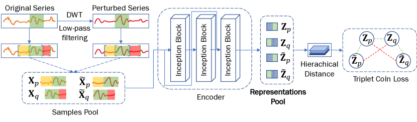
Figure 1: Overview of the proposed CoInception framework. We use samples from Representation Pool in different downstream tasks.

2.2.1 Sampling Strategy

To guarantee the reliability of the results, we strive to preserve the distinctiveness of the acquired representations when the input sequences are exposed to diverse contexts (i.e., contextual consistency [65]). Although ensuring contextual consistency has been demonstrated to be more robust than previous consistencies [17, 18, 55], we recognize a circumstance that none of the previous works have taken into account: the noise-vulnerability of time series’ learned representations.

Natural time series often contain noise, represented as a random process that oscillates independently alongside the main signal (e.g., white noise [40, 39]). We express a time series signal $\mathbf{x}$ as $\mathbf{x}=\mathbf{\hat{x}}+\mathbf{n}$, where $\mathbf{\hat{x}}$ depicts the original signal and $\mathbf{n}$ represents an independent noise component. While existing approaches treat the signal and noise separately when only the noise factor varies (e.g., $\mathbf{n}\rightarrow\mathbf{\tilde{n}}$), we argue that the noise-like elements, which appear as high-frequency components in the original series [28, 37], provide little to no meaningful information, and may degrade the accuracy of the downstream tasks severely. Therefore, it is crucial for our learned representations to be resilient to these random high-frequency signals, referred to as noise resiliency.

Figure 2 illustrates the effect of ensuring the noise resiliency through the representations learned by our CoInception framework and those produced by TS2Vec [65]. For demonstration, we generate a toy series that is originally a sine wave with two noise signals of different frequencies added at the two end segments and a level shift with increasing amplitude (Amp) in the middle range (Figure 2 - upper). The CoInception model’s representations (Fig. 2(b)) neglect the high-frequency noise and capture the harmonic change in the original series over all the latent dimensions (Dim) while also producing different representations for segments with a level shift. On the other hand, the representations produced by TS2Vec (Fig. 2(a)) are less interpretable due to the effect of noise, and there is no apparent similarity between the representations of the two end segments.

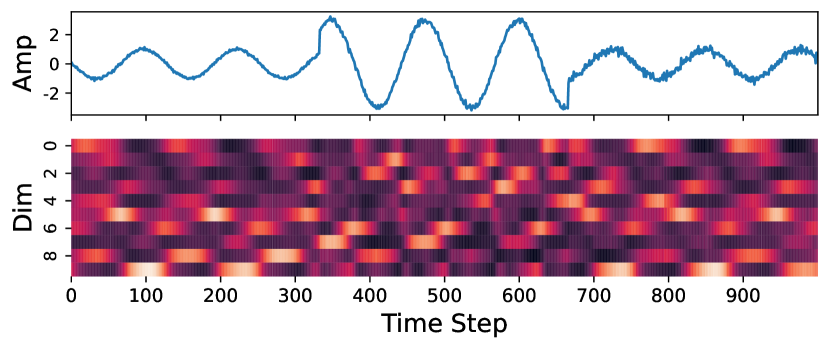
(a) TS2Vec

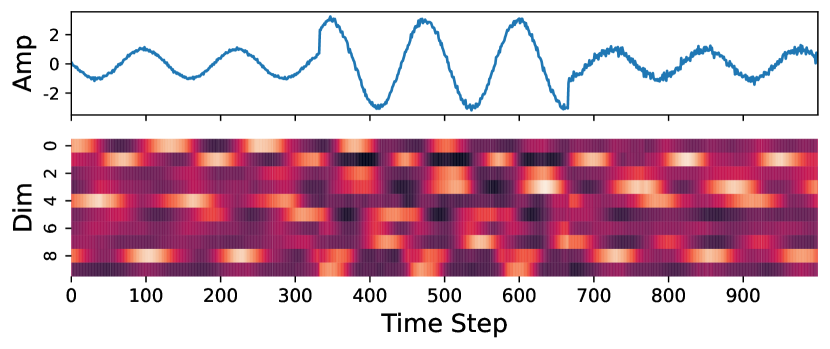
(b) CoInception (our)

Figure 2: Output representations for toy time series containing high-frequency noise. CoInception’s results can still capture the periodic characteristics regardless of the presence of noise.

Figure 1 depicts an overview of the proposed sampling strategy. We introduce a parameter-free Discrete Wavelet Transform (DWT) low-pass filter [48] to generate a perturbed version $\mathbf{\tilde{x}}$ of the original series $\mathbf{x}$, for enhancing the noise resilience. The DWT filter convolves the time series with wavelet functions to generate coefficients representing the contribution of wavelet functions at various intervals. The low-frequency approximation coefficients reflect the overall trend of the data, whereas the high-frequency detail coefficients represent noise-like components. By repeatedly employing the low-pass filter, the time series is segregated into distinct frequency bands. Let $\mathbf{g}$ and $\mathbf{h}$ be the low-pass and high-pass filters, respectively. We represent the mathematical operation of the DWT low-pass and high-pass filters for decomposing $\mathbf{x}$ at level $j$ and position $n$ as follows.

$$\mathbf{x}^{j}[n]=(\mathbf{x}^{j-1}*\mathbf{g}^{j})[n]=\sum_{k}\mathbf{x}^{j-1}[k]\mathbf{g}^{j}[2n-k],~{}~{}\mathbf{d}^{j}[n]=(\mathbf{x}^{j-1}*\mathbf{h}^{j})[n]=\sum_{k}\mathbf{x}^{j-1}[k]\mathbf{h}^{j}[2n-k],$$

where $*$ represents convolution operator, $\mathbf{x}^{j}$ and $\mathbf{d}^{j}$ are the approximation and detail coefficients, $\mathbf{g}^{j}$ and $\mathbf{h}^{j}$ represent the low-pass and high-pass filter coefficients. $j$ indicates the level index, and $k$ denotes the shifted coefficient. We repeat the recursive filtering process until reaching the maximum useful level of the decomposition $L=\lfloor\log_{2}(\tfrac{M}{K})\rfloor$, where $K$ is the length of the mother wavelet. Following, to create a perturbed version of the input series, we first retain only the significant values in the detail coefficients $\mathbf{d}^{j}$ ($j\in\left\{1,\dots,L\right\}$), while masking out unnecessary (potentially noise) values, which result in perturbed detail coefficients $\mathbf{\tilde{d}}^{j}$ as follows.

$$\begin{split}\mathbf{\tilde{d}}^{j}&=\left[\frac{d_{k}}{|d_{k}|\times\max(|d_{k}|-\gamma,0)}\text{ if }d_{k}>\gamma\text{ else }0\Big{|}k\in\left\{1,2,\dots,\text{len}(\mathbf{d}^{j})\right\}\right].\end{split}$$ (1)

With this strategy, we define a cutting threshold $\gamma$ to be proportional to the maximum value of the input series $\mathbf{x}$ by a hyper-parameter $\alpha<1$, i.e., $\gamma=\alpha\times\max(\mathbf{x})$. After that, the reconstructions of approximation coefficient $\mathbf{\mathbf{x}^{L}}$ and set of perturbed detail coefficients $\left\{\mathbf{\tilde{d}}^{1},\dots,\mathbf{\tilde{d}}^{L}\right\}$ with invert DWT result the perturbed series $\mathbf{\tilde{x}}$. We describe details of this reconstruction process in the Appendix. Once achieved perturbed input series $\mathbf{\tilde{x}}$, to ensure contextual consistency, we adopt the technique proposed in TS2Vec [65] to sample overlapping segments $\left<\mathbf{x}_{p};\mathbf{x}_{q}\right>$ and $\left<\mathbf{\tilde{x}}_{p};\mathbf{\tilde{x}}_{q}\right>$ from $\mathbf{x}$ and $\mathbf{\tilde{x}}$ to create negative and positive pairs (see Section 2.3). Then we feed these four segments into CoInception’s encoder framework (see Section 2.2.2).

2.2.2 Inception-Based Dilated Convolution Encoder

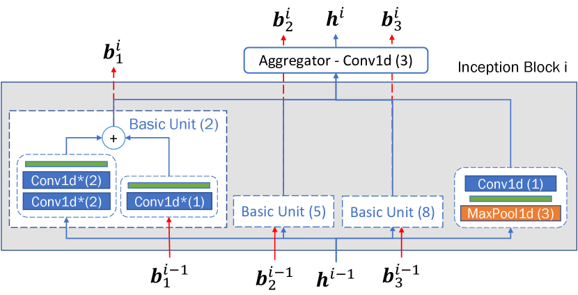
(a) Inception Block

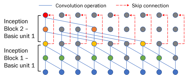
(b) Receptive field illustration

Figure 3: Illustration of the Inception block and the accumulated receptive field upon stacking.

To ensure robustness and scalability, our CoInception encoder has a stack of Inception blocks, each containing multiple Basic units of varying scales (Fig.3(a)). In contrast to existing Inception-based models, e.g., InceptionTime [22], we introduce three simple yet effective modifications: (1) an aggregator layer, (2) dilated convolution (Conv1d* in Fig. 3(a)), and (3) extra skip connections (i.e., red arrows in Fig. 3(b)). These modifications enable us to achieve our desired principles without sacrificing implementation simplicity.

The Inception block, depicted in Fig. 3(a), consists of multiple Basic units comprising 1D convolutional layers with variable filter lengths, allowing us for considering input segments at various scales and resolutions. The outputs of these layers are concatenated and passed through an aggregator, which is another 1D convolutional layer. Beyond reducing the number of parameters as in [52, 22], our aggregator is intentionally placed after the Basic units to better combine the features produced by those layers, rather than simple concatenation. Moreover, with the stacking nature of Inception blocks in our design, the aggregator can still inherit the low-channel-dimension output of the previous block, which has the same effect as the conventional Bottleneck layer.

To further enhance the scalability and efficiency, we employ stacked dilated convolution layers with incremental dilation factors inside the Basic units, along with additional skip connections between those units’ outputs of different Inception blocks. In this way, our CoInception framework can be seen as a set of multiple dilated convolution experts, with much shallower depth and equivalent receptive fields compared with ordinary stacked Dilated Convolution networks [18, 65]. Moreover, the skip connections serve as a skip link for stable gradient flow and gluing up the Basic units of different Inception blocks, making the entire encoder horizontally and vertically connected.

Specifically, we use three Basic units for each Inception block, each consisting of two similar convolution layers with a base kernel size. Let $k_{u}$ be the base kernel size for such a layer in Basic unit $u$, in the $i^{th}$ Inception block ($1$-indexed), the dilation factor and the receptive field are calculated as $d_{u}^{i}=(2k-1)^{i-1};r_{u}^{i}=(2k-1)^{i}$. Figure 3(b) represents the cumulative receptive field corresponding to Basic unit $\mathbf{b}_{1}$ with the base kernel size of $2$ at the first and second Inception blocks. With this design, the CoInception encoder does not need to go deep vertically, ensuring better gradient flow and still achieving comparable receptive fields compared to dilated convolution networks, while having significantly fewer parameters to be learned. The detailed analysis of the relationship between the number of layers and the receptive field are presented in the Appendix - Further Experiment Results and Analysis.

2.3 Hierarchical Triplet Loss

In addition to the sampling strategy described in Section 2.2.1, we propose a novel loss function combining ideas from hierarchical loss [65] and triplet loss [7, 20] to achieve both contextual consistency and noise resilience. Specifically, let $\mathbf{x}_{p}$ and $\mathbf{x}_{q}$ be the two overlapped segments derived from the same time series, and $\mathbf{\tilde{x}}_{p}$ and $\mathbf{\tilde{x}}_{q}$ be their perturbed views. We aim to make the learned embeddings $\mathbf{z}_{p}$ and $\mathbf{z}_{q}$ close in latent space to preserve the contextual consistency. Moreover, we minimize the distance between the representations of the original segments and their perturbed views - $\left<\mathbf{z}_{p};\mathbf{\tilde{z}}_{p}\right>$ and $\left<\mathbf{z}_{q};\mathbf{\tilde{z}}_{q}\right>$ to generate noise-resilient representations. Similar to [65], we incorporate both instance-wise loss [18] ($\mathcal{L}_{ins}$) and temporal loss [55] ($\mathcal{L}_{temp}$) to model the distance within a couplet. The combination of these two losses forms the contextual loss $\mathcal{L}_{con}$.

$$\begin{split}\mathcal{L}_{temp}(\mathbf{z}_{p},\mathbf{z}_{q})&=\tfrac{1}{BT}\sum^{B}_{b}\sum^{T}_{t}-\log\tfrac{\exp(z^{b,t}_{p}\cdot z^{b,t}_{q})}{\sum^{T}_{\tilde{t}}\left(\exp(z^{b,t}_{p}\cdot z^{b,\tilde{t}}_{q})+\mathbbm{1}_{t\neq\tilde{t}}\exp(z^{b,t}_{p}\cdot z^{b,\tilde{t}}_{p})\right)},\\ \mathcal{L}_{ins}(\mathbf{z}_{p},\mathbf{z}_{q})&=\tfrac{1}{BT}\sum^{B}_{b}\sum^{T}_{t}-\log\tfrac{\exp(z^{b,t}_{p}\cdot z^{b,t}_{q})}{\sum^{B}_{\tilde{b}}\left(\exp(z^{b,t}_{p}\cdot z^{\tilde{b},t}_{q})+\mathbbm{1}_{b\neq\tilde{b}}\exp(z^{b,t}_{p}\cdot z^{\tilde{b},t}_{p})\right)},\\ \mathcal{L}_{con}(\mathbf{z}_{p},\mathbf{z}_{q})&=\mathcal{L}_{temp}(\mathbf{z}_{p},\mathbf{z}_{q})+\mathcal{L}_{ins}(\mathbf{z}_{p},\mathbf{z}_{q}).\end{split}$$

We apply similar formulas for $\mathcal{L}_{con}(\mathbf{z}_{p},\mathbf{\tilde{z}}_{p})$ and $\mathcal{L}_{con}(\mathbf{z}_{q},\mathbf{\tilde{z}}_{q})$. Furthermore, our objective is to enhance the reliability of learned representations based on the following observation. Besides the three couplets mentioned earlier, there are extra pairs that can be created by comparing the representations of a vanilla segment and a perturbed version in a different context, e.g. $\left<\mathbf{z}_{p};\mathbf{\tilde{z}}_{q}\right>$. We argue that $\mathbf{z}_{p}$ should be closer to the vanilla representation $\mathbf{z}_{q}$ compared to its perturbed view $\mathbf{\tilde{z}}_{q}$. We incorporate this observation as a constraint in the final loss function (denoted as $\mathcal{L}_{triplet}$) in the format of a triplet loss as follows.

$$\mathcal{L}_{triplet}(l_{pq},l_{p\tilde{q}},l_{\tilde{p}q},\epsilon,\zeta)=\epsilon\times\tfrac{l_{pq}+l_{p\tilde{p}}+l_{q\tilde{q}}}{3}+(1-\epsilon)\times\max(0,2\times l_{pq}-l_{p\tilde{q}}-l_{\tilde{p}q}+2\times\zeta),$$ (2)

where $l_{pq}$ represents $\mathcal{L}_{con}(\mathbf{z}_{p},\mathbf{z}_{q})$ and we apply similar notations for the others. The parameter $\epsilon<1$ is a balance factor for two loss terms, while $\zeta$ denotes the triplet margin. To ensure the CoInception framework can handle inputs of multiple granularity levels, we adopt a hierarchical strategy similar to [65] with our $\mathcal{L}_{triplet}$ loss. We describe the details in Appendix - Algorithm 1.

3 Experiments

In this section, we empirically validate the effectiveness of the CoInception framework and compare the results with the recent state of the arts. We consider three major tasks, including forecasting, classification, and anomaly detection, as in Section 2.1. Our evaluation encompasses multiple benchmarks, some of which also target multiple tasks: (1) TS2Vec [65] learns to preserve contextual invariance across multiple time resolutions using a sampling strategy and hierarchical loss; (2) TS-TCC [17] is a self-supervised learning approach combining cross-view prediction and contrastive learning tasks by creating two views of the raw time series data using weak and strong augmentations; (3) TNC [55] is a contrastive learning method tailored for time series data that forms positive and negative pairs from nearby and distant segments, respectively, leveraging the stationary properties of time series.

3.1 Time-Series Forecasting

Datasets & Settings. For this experiment, the same settings as described in [69] are adopted for both short-term and long-term forecasting. The supervised benchmark model used is the Informer [69], while for other unsupervised benchmarks, a linear regression model is trained using the $L2$ norm penalty, with the learned representation $\mathbf{z}$ as input to directly predict future values. To ensure a fair comparison with works that only generate segment-level representations, only the $M^{th}$ timestep representation $z^{M}$ produced by the CoInception framework is used for the input segment. The evaluation of the forecast result is performed using two metrics, namely Mean Square Error (MSE) and Mean Absolute Error (MAE). For the datasets used, the Electricity Transformer Temperature (ETT) [69] datasets are adopted together with the UCR Electricity [1] dataset. In addition to the representative works, CoInception is further compared with studies that delicately target the forecasting task, such as Informer [69], StemGNN [5], LogTrans [31], N-BEATS [38], and LSTnet [27].

Table 1: Multivariate time series forecasting results.

Dataset	Length	TS2Vec		TS-TCC		TNC		Informer		StemGNN		LogTrans		CoInception
		MSE	MAE	MSE	MAE	MSE	MAE	MSE	MAE	MSE	MAE	MSE	MAE	MSE	MAE
	24	0.599	0.534	0.653	0.610	0.632	0.596	0.577	0.549	0.614	0.571	0.686	0.604	0.461	0.479
	48	0.629	0.555	0.720	0.693	0.705	0.688	0.685	0.625	0.748	0.618	0.766	0.757	0.512	0.503
	168	0.755	0.636	1.129	1.044	1.097	0.993	0.931	0.752	0.663	0.608	1.002	0.846	0.683	0.601
	336	0.907	0.717	1.492	1.076	1.454	0.919	1.128	0.873	0.927	0.730	1.362	0.952	0.829	0.678
ETTh1	720	1.048	0.790	1.603	1.206	1.604	1.118	1.215	0.896	-	-	1.397	1.291	1.018	0.770
	24	0.398	0.461	0.883	0.747	0.830	0.756	0.720	0.665	1.292	0.883	0.828	0.750	0.335	0.432
	48	0.580	0.573	1.701	1.378	1.689	1.311	1.457	1.001	1.099	0.847	1.806	1.034	0.550	0.560
	168	1.901	1.065	3.956	2.301	3.792	2.029	3.489	1.515	2.282	1.228	4.070	1.681	1.812	1.055
	336	2.304	1.215	3.992	2.852	3.516	2.812	2.723	1.340	3.086	1.351	3.875	1.763	2.151	1.188
ETTh2	720	2.650	1.373	4.732	2.345	4.501	2.410	3.467	1.473	-	-	3.913	1.552	2.962	1.338
	24	0.443	0.436	0.473	0.490	0.429	0.455	0.323	0.369	0.620	0.570	0.419	0.412	0.384	0.423
	48	0.582	0.515	0.671	0.665	0.623	0.602	0.494	0.503	0.744	0.628	0.507	0.583	0.552	0.521
	168	0.622	0.549	0.803	0.724	0.749	0.731	0.678	0.614	0.709	0.624	0.768	0.792	0.561	0.533
	336	0.709	0.609	1.958	1.429	1.791	1.356	1.056	0.786	0.843	0.683	1.462	1.320	0.623	0.578
ETTm1	720	0.786	0.655	1.838	1.601	1.822	1.692	1.192	0.926	-	-	1.669	1.461	0.717	0.639
	24	0.287	0.374	0.278	0.370	0.305	0.384	0.312	0.387	0.439	0.388	0.297	0.374	0.234	0.335
	48	0.307	0.388	0.313	0.392	0.317	0.392	0.392	0.431	0.413	0.455	0.316	0.389	0.265	0.356
	168	0.332	0.407	0.338	0.411	0.358	0.423	0.515	0.509	0.506	0.518	0.426	0.466	0.282	0.372
	336	0.349	0.420	0.357	0.424	0.349	0.416	0.759	0.625	0.647	0.596	0.365	0.417	0.301	0.388
Electricity	720	0.375	0.438	0.382	0.442	0.447	0.486	0.969	0.788	-	-	0.344	0.403	0.331	0.409

Results. Due to limited space, we only present the multivariate forecasting results in Table 1, while the results for the univariate scenario can be found in the Appendix. For better comparison, in all of our experiments, we highlight best results in bold and red, and second best results are in blue. Apparently, the proposed CoInception framework achieves the best results in most scenarios over all 4 datasets in the multivariate setting. The numbers indicate that our method outperforms existing state-of-the-art methods in most cases. Furthermore, the Inception-based encoder design results in a CoInception model with only $40\%$ number of parameters compared with the second-best approach (see Table 2).

3.2 Time-Series Classification

Datasets & Settings. For the classification task, we follow the settings in [18] and train an RBF SVM classifier on segment-level representations generated by our baselines. However, since the CoInception model produces instance-level representations for each timestep similar to TS2Vec [65], we utilize the strategy from [65] to ensure a fair comparison. Specifically, we apply a global MaxPooling operation over $\mathbf{z}$ to extract the segment-level vector representing the input segment. We assess the performance of all models using two metrics: prediction accuracy and the area under the precision-recall curve (AUPRC). We test the proposed approach against multiple benchmarks on two widely used repositories: the UCR Repository [11] with 128 univariate datasets and the UEA Repository [2] with 30 multivariate datasets. To further strengthen our empirical evidence, we additionally implement a K-nearest neighbor classifier equipped with DTW [9] metric, along with T-Loss [18] and TST [66] beside the aforementioned SOTA approaches.

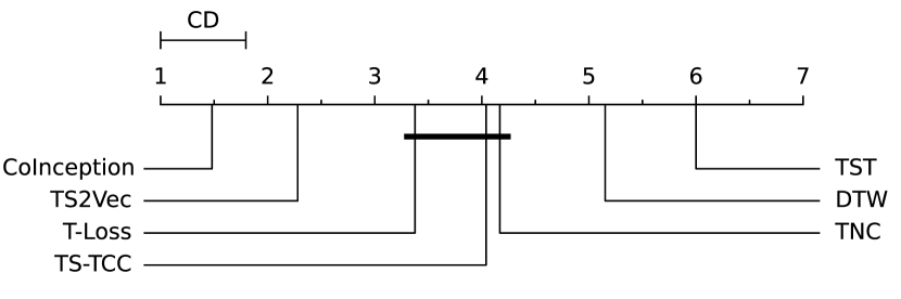
Figure 4: Critical Difference Diagram comparing different classifiers on 125 Datasets from UCR Repository with the confidence level of $95\%$.

Table 2: Time series classification results.

Dataset	UCR repository			UEA repository
	Accuracy	Rank	Parameter	Accuracy	Rank	Parameter
DTW	0.72	5.15	-	0.65	3.86	-
TNC	0.76	4.17	462K∗	0.68	4.58	462K∗
TST	0.64	6.00	2.88M	0.64	5.27	2.88M
TS-TCC	0.76	4.04	1.44M	0.68	3.86	1.44M
T-Loss	0.81	3.38	247K	0.67	3.75	247M
TS2Vec	0.83	2.28	641K	0.71	2.96	641K
CoInception	0.84	1.48	206K	0.72	1.89	206K
x‘1

Results. The evaluation results of our proposed CoInception framework on the UCR and UEA repositories are presented in Table 2. Details for individual datasets are in the Appendix. For 125 univariate datasets in the UCR repository, CoInception ranks first in a majority of 86 datasets, and for 29 UEA datasets it produces the best classification accuracy in 16 datasets. In this table, we also add a detailed number of parameters for every framework when setting a fixed latent dimension of $320$. With the fusion of dilated convolution and Inception strategy, CoInception achieves the best performance while being much more lightweight ($2.35$ times) than the second best framework - here TS2Vec [65]. We also visualize the critical difference diagram [14] for the Nemenyi tests on 125 UCR datasets in Figure 4. Intuitively, in this diagram, classifiers connected by a bold line indicate a statistically insignificant difference in average ranks. As suggested, CoInception makes a clear improvement gap compared with other SOTAs in average ranks.

3.3 Time-Series Anomaly Detection

Datasets & Settings. For this task, we adopt the protocols introduced by Ren et al. [44] and Zhihan et al. [65]. However, we make three forward passes during the evaluation process, which is different from [65]. In the first pass, we mask $x^{M}$ and generate the corresponding representation ${z}^{M}_{1}$, as CoInception has learned to preserve the contextual invariance. The second pass puts the input segment $\mathbf{x}$ through our DWT low-pass filter (Section 2.2.1) to generate the softened segment $\tilde{\mathbf{x}}$, before getting the representation ${z}^{M}_{2}$. The normal input is used in the last pass, and ${z}^{M}_{3}$ is its corresponding output. Accordingly, we define the abnormal score as $\alpha_{M}=\frac{1}{2}\left(\lVert z^{M}_{1}-z^{M}_{3}\rVert_{1}+\lVert z^{M}_{2}-z^{M}_{3}\rVert_{1}\right)$. We keep the remaining settings intact as [44, 65] for both normal and cold-start experiments. Precision (P), Recall (R), and F1 score (F1) are used to evaluate anomaly detection performance. We use the Yahoo dataset [29], a benchmark dataset consisting of 367 segments labeled with anomalous points, and the KPI dataset [44] from the AIOPS Challenge. Additionally, we compare CoInception with other SOTA unsupervised methods that are utilized for detecting anomalies, such as SPOT [47], DSPOT [47], DONUT [63], and SR [44] for normal detection tasks, as well as FFT [43], Twitter-AD [57], and Luminol [32] for cold-start detection tasks that require no training data.

Table 3: Time series abnormaly detection results.

Dataset	Metrics	Normal Setting						Cold-start Setting
		SPOT	DSPOT	DONUT	SR	TS2Vec	CoInception	FFT	Twitter-AD	Luminol	SR	TS2Vec	CoInception
Yahoo	F1	0.338	0.316	0.026	0.563	0.745	0.769	0.291	0.245	0.388	0.529	0.726	0.745
	Precision	0.269	0.241	0.013	0.451	0.729	0.790	0.202	0.166	0.254	0.404	0.692	0.733
	Recall	0.454	0.458	0.825	0.747	0.762	0.748	0.517	0.462	0.818	0.765	0.763	0.754
KPI	F1	0.217	0.521	0.347	0.622	0.677	0.681	0.538	0.330	0.417	0.666	0.676	0.682
	Precision	0.786	0.623	0.371	0.647	0.929	0.933	0.478	0.411	0.306	0.637	0.907	0.893
	Recall	0.126	0.447	0.326	0.598	0.533	0.536	0.615	0.276	0.650	0.697	0.540	0.552

Results. Table 3 presents a performance comparison of various methods on the Yahoo and KPI datasets using F1 score, precision, and recall metrics. We observe that CoInception outperforms existing SOTAs in the main F1 score for all two datasets in both the normal setting and the cold-start setting. In addition, CoInception also reveals its ability to perform transfer learning from one dataset to another, through steady enhancements in the empirical result for cold-start settings. This transferability characteristic is potentially a key to attaining a general framework for time series data. Futher experiments for investigating this are presented in the Appendix.

4 Analysis

4.1 Ablation Analysis

In this experiment, we analyze the impact of different components on the overall performance of the CoInception framework. We created three variations: (1) W/o noise resilient sampling inherits the sampling strategy and hierarchical loss from [65]; (2) W/o Dilated Inception block uses a stacked Dilated Convolution network instead of our CoInception encoder; and (3) W/o triplet loss removes the triplet-based term from our $\mathcal{L}_{triplet}$ calculation. Results are summarized in Table 4. Overall, there is a significant performance decline in all three versions for the main time series tasks. Without noise resilient sampling, performance drops from $8\%$ in classification to $15\%$ in anomaly detection. Removing the Dilated Inception-based encoder leads to up to $9\%$ performance drop in anomaly detection while eliminating the triplet loss results in performance reductions of $4-17\%$.

Table 4: Ablation analysis for the proposed CoInception framework.

Task		W/o noise resilient sampling	W/o Dilated Inception block	W/o triplet loss	Full version
	Acc.	0.645 (-8.51%)	0.661 (-6.24%)	0.624 (-11.48%)	0.705
Classification	AUC.	0.704 (-9.04%)	0.726 (-6.20%)	0.691 (-10.72%)	0.774
	MSE	0.067 (-8.95%)	0.065 (-6.15%)	0.064 (-4.68%)	0.061
Forecasting	MAE	0.178 (-2.81%)	0.180 (-3.88%)	0.177 (-2.26%)	0.173
	F1	0.646 (-15.99%)	0.704 (-8.45%)	0.636 (-17.29%)	0.769
	P.	0.607 (-23.16%)	0.720 (-8.86%)	0.581 (-26.45%)	0.790
Anomaly Detection	R.	0.692 (-7.48%)	0.689 (-7.88%)	0.701 (-6.28%)	0.748

4.2 Alignment and Uniformity

We assess the learned representations via two qualities: Alignment and Uniformity, as proposed in [61]. Alignment measures feature similarity across samples, ensuring insensitivity to noise in positive pairs. Uniformity aims to retain maximum information by minimizing the intra-similarities of positive pairs and maximizing inter-distances of negative pairs while maintaining a uniform feature distribution.

Figure 5 summarizes the distributions of testing set features for the StarLightCurves dataset generated by CoInception and TS2Vec. Generally, CoInception’s features exhibit a more uniform distribution and are particularly more closely clustered for positive pairs. The first column shows the distance distribution between features of positive pairs, with CoInception having smaller mean distances and decreasing bin heights as distance increases, unlike TS2Vec. For the remaining columns, we plot feature distributions using Gaussian kernel density estimation (KDE) and von Mises-Fisher (vMF) KDE for angles. CoInception demonstrates superior uniform characteristics for the entire test set representation, as well as better clustering between classes. Representations of different classes reside on different segments of the unit circle.

(a) CoInception

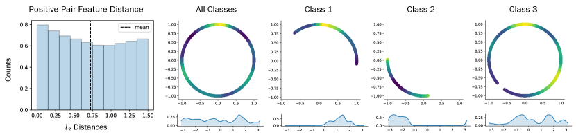
(b) TS2Vec

Figure 5: Alignment analysis. Distribution of $l_{2}$ distance between features of positive pairs. Uniformity analysis. Feature distributions with Gaussian kernel density estimation (KDE) (above) and von Mises-Fisher (vMF) KDE on angles (below).

5 Conclusion

We introduce CoInception, a novel framework designed to tackle the challenges of robust and efficient time series representation learning. Our approach generates representations that are resilient to noise by utilizing a DWT low-pass filter. By incorporating Inception blocks and dilation concepts into our encoder framework, we strike a balance between robustness and efficiency. CoInception empirically outperforms state-of-the-art methods across a range of time series tasks including forecasting, classification and abnormality detection. Moreover, CoInception achieves first place rankings on the majority of the classification UCR datasets. These findings contribute to the advancement of foundational frameworks for time series data. For future work, we aim to explore the transferability of our approach and enhance its foundational characteristics for time series analysis.

CoInception Supplement Details

Sampling Strategy

This section cover the working of invert DWT low-pass filter [48] to reconstruct perturbed series $\mathbf{\tilde{x}}$. This process involves combining the approximation coefficients $\mathbf{\mathbf{x}^{L}}$ and perturbed detail coefficients $\left\{\mathbf{\tilde{d}}^{1},\dots,\mathbf{\tilde{d}}^{L}\right\}$ obtained during the decomposition process.

By utilizing the inverse low-pass and high-pass filters, the original signal can be reconstructed from these coefficients. Let $\mathbf{\tilde{g}}$ and $\mathbf{\tilde{h}}$ represent these low- and high-pass filters, respectively. The mathematical operations for the DWT reconstruction filters, which recover the perturbed signal $\mathbf{\tilde{x}}$ at level $j$ and position $n$, can be represented as follows:

$$\mathbf{\tilde{x}}^{j-1}[n]=(\mathbf{\hat{x}}^{j}\ast\mathbf{\tilde{g}}^{j})[n]+(\mathbf{\tilde{d}}^{j}\ast\mathbf{\tilde{h}}^{j})[n]=\sum_{k}\mathbf{\hat{x}}^{j}[2n-k]\mathbf{\tilde{g}}^{j}[k]+\sum_{k}\mathbf{\tilde{d}}^{j}[2n-k]\mathbf{\tilde{h}}^{j}[k],\\$$

where

$$\begin{cases}\mathbf{\tilde{x}}^{L}&=\mathbf{x}^{L}\\ \mathbf{\hat{x}}^{j}&=\texttt{Upsampling}(\mathbf{\tilde{x}}^{j},2).\end{cases}$$

In these equations, $\mathbf{\hat{x}}^{j}$ represents the upsampled approximation at level $j$. The upsampling process Upsampling involves inserting zeros between the consecutive coefficients to increase their length, effectively expanding the signal toward the original length of input series. Following, the upsampled coefficients are convolved with the corresponding reconstruction filters $\mathbf{\tilde{g}}^{j}$ and $\mathbf{\tilde{h}}^{j}$ to obtain the reconstructed signal $\mathbf{\tilde{x}}^{j-1}$ at the previous level.

This recursive filtering and upsampling process is repeated until the maximum useful level of decomposition, $L=\lfloor\log_{2}(\tfrac{M}{K})\rfloor$, is reached. Here, $M$ represents the length of the original signal and $K$ is the length of the mother wavelet. By iteratively applying the reconstruction filters and combining the coefficients obtained after upsampling, the original signal can be reconstructed, gradually restoring both the overall trend (approximation) and the high-frequency details captured by the DWT decomposition.

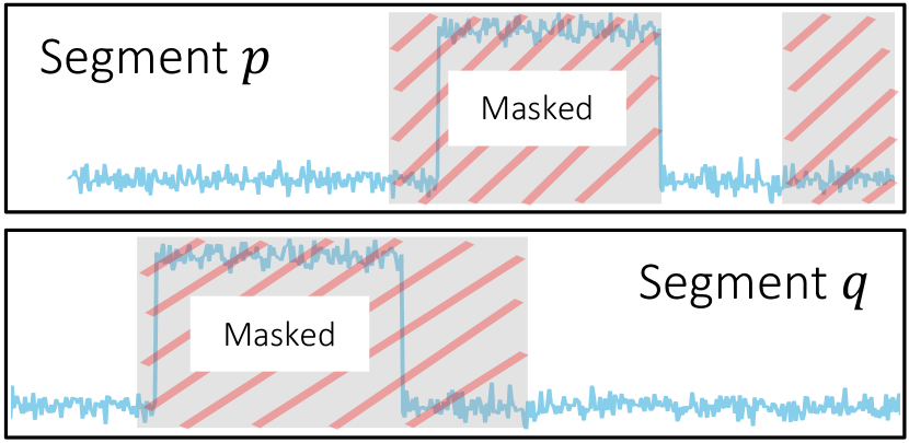
Figure 6: Temporal Masking collapse. An illustration for a case in which temporal masking would hinder training progress.

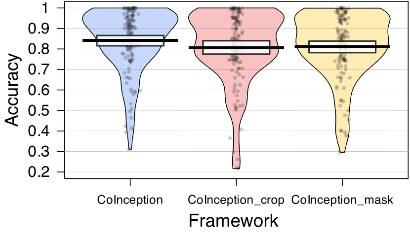
Figure 7: Ablation in sampling strategy. Accuracy distribution of different variants over 128 UCR dataset.

To maintain the characteristic of context invariance, we employ a different approach than TS2Vec [65]. We have chosen to rely solely on random cropping for generating overlapping segments, without incorporating temporal masking. This decision is based on recognizing several scenarios that could undermine the effectiveness of this strategy. Firstly, if heavy masking is applied, it may lead to a lack of explicit context information. The remaining context information, after extensive occlusion, might be insufficient or unrepresentative for recovering the masked timestamp, thus impeding the learning process. Secondly, when dealing with data containing occasional abnormal timestamps (e.g., level shifts), masking these timestamps in both overlapping segments (Figure 7) can also hinder the learning progress since the contextual information becomes non-representative for inference.

According to the findings discussed in [65], random cropping is instrumental in producing position-agnostic representations, which helps prevent the occurrence of representation collapse when using temporal contrasting. This is attributed to the inherent capability of Convolutional networks to encode positional information in their learned representations [21, 8], thereby mitigating the impact of temporal contrasting as a learning strategy. As the Inception block in CoInception primarily consists of Convolutional layers, the adoption of random cropping assumes utmost importance in enabling CoInception to generate meaningful representations.

The accuracy distribution for 128 UCR datasets across various CoInception variations is illustrated in Figure 7. These variations include: (1) the ablation of Random Cropping, where two similar segments are used instead, and (2) the inclusion of temporal masking on the latent representations, following the approach in [65]. As depicted in the figure, both variations exhibit a decrease in overall performance and a higher variance in accuracy across the 128 UCR datasets, compared with our proposed framework.

Inception-Based Dilated Convolution Encoder

While the main structure of our CoInception Encoder is a stack of Inception blocks, there are some additional details discussed in this section.

Before being fed into the first Inception block, the input segments are first projected into a different latent space, other than the original feature space. We intentionally perform the mapping with a simple Fully Connected layer.

$$\begin{split}&\theta:\mathbb{R}^{M\times N}\rightarrow\mathbb{R}^{M\times K}\\ &\theta(\mathbf{x})=\mathbf{W}\mathbf{x}+\mathbf{b}\end{split}$$

The benefits of this layer are twofold. First, upon dealing with high-dimensional series, this layer essentially act as a filter for dimensionality reduction. The latent space representation retains the most informative features of the input segment while discarding irrelevant or redundant information, reducing the computational burden on the subsequent Inception blocks. This layer make CoInception more versatile to different datasets, and ensure its scalability. Second, the projection by Fully Connected layer help CoInception enhance its transferability. Upon adapting the framework trained with one dataset to another, we only need to retrain the projection layer, while keeping the main stacked Inception layers intact.

To provide a clearer understanding of the architecture depicted in Inception block 3(a), we will provide a detailed interpretation. In our implementation, each Inception block consists of three Basic units. Let the outputs of these units be denoted as $\mathbf{b}_{1}$, $\mathbf{b}_{2}$, and $\mathbf{b}_{3}$. To enhance comprehension, we will use the notation $\mathbf{b}_{j}$ to represent these three outputs collectively. Additionally, we will use $\mathbf{m}$ to denote the output of the Maxpooling unit, and $\mathbf{h}$ to represent the overall output of the entire Inception block. The following formulas outline the operations within the $i^{th}$ Inception block.

$$\begin{split}\mathbf{b}_{k}^{i}&=\texttt{Conv1d*}(\sigma(\texttt{Conv1d*}(\mathbf{h}^{i-1})))+\sigma(\texttt{Conv1d*}(\mathbf{b}^{i-1}_{k})),\\ \mathbf{m}^{i}&=\sigma(\texttt{Conv1d*}(\mathbf{b}^{i-1}_{k})),\\ \mathbf{h}^{i}&=\texttt{Aggregator}(\texttt{Concat}(\mathbf{b}_{k}^{i},\mathbf{m}^{i})).\end{split}$$ (3)

In these equations, $\sigma$ represent the LeakyReLU activation function, which is used throughout the CoInception architecture.

Hierarchical Triplet Loss

Algorithm 1 describe the procedure to calculate the hierarchical triplet loss mentioned in the manuscript. With this loss, we cover and maintain the objectives set out in various resolutions of input time series.

Algorithm 1 Hierarchical Triplet Loss Calculation

Input:
$\triangleright\hskip 5.69046pt\mathbf{z}_{i},\mathbf{z}_{j}$ - latent representations of $i^{th}$ and $j^{th}$ segments;
$\triangleright\hskip 5.69046pt\mathbf{\tilde{z}}_{i},\mathbf{\tilde{z}}_{j}$ - latent representations of $i^{th}$ and $j^{th}$ perturbed segments;
$\triangleright\hskip 5.69046pt\epsilon$ - Balance factor between instance loss and temporal loss;
$\triangleright\hskip 5.69046pt\zeta$ - Triplet loss margin.
Output:
$\triangleright\hskip 5.69046ptl_{3hier}$ - Hierarchical triplet loss value

1:0function HierTripletLoss()

2:-1Initialize $l_{3hier}\leftarrow 0$; $r\leftarrow 0$ $\triangleright$ Running variable

3:-2$\texttt{time\_dimension}(\mathbf{z}_{i})>1$ $\triangleright$ Loop with reduced time resolution

4:-3$l_{ij};l_{i\tilde{i}};l_{j\tilde{j}}\leftarrow\mathcal{L}_{con}(\mathbf{z}_{i},\mathbf{z}_{j});\mathcal{L}_{con}(\mathbf{z}_{i},\mathbf{z}_{\tilde{i}});\mathcal{L}_{con}(\mathbf{z}_{j},\mathbf{z}_{\tilde{j}})$; $\triangleright$ Losses for main couplets

5:

6:-4$l_{i\tilde{j}};l_{\tilde{i}j}\leftarrow\mathcal{L}_{con}(\mathbf{z}_{i},\mathbf{z}_{\tilde{j}});\mathcal{L}_{con}(\mathbf{z}_{\tilde{i}},\mathbf{z}_{j})$; $\triangleright$ Losses for supporting couplets

7:

8:-5$l_{3hier}\leftarrow l_{3hier}+\mathcal{L}_{triplet}(l_{ij},l_{i\tilde{j}},l_{\tilde{i}j},\epsilon,\zeta)$;

9:

10:

11:-6$\mathbf{z}_{i}\leftarrow\texttt{max\_pool\_1d}(\mathbf{z}_{i})$; $\mathbf{z}_{j}\leftarrow\texttt{max\_pool\_1d}(\mathbf{z}_{j})$ $\triangleright$ Reducing the time resolution

12:

13:-7$\mathbf{\tilde{z}}_{i}\leftarrow\texttt{max\_pool\_1d}(\mathbf{\tilde{z}}_{i})$; $\mathbf{\tilde{z}}_{j}\leftarrow\texttt{max\_pool\_1d}(\mathbf{\tilde{z}}_{j})$

14:

15:-8$d\leftarrow d+1$

16:-9

17:-10$l_{3hier}\leftarrow l_{3hier}/d$

18:-11return $l_{3hier}$

19:-12

Implementation Details

Environment Settings

All implementations and experiments are performed on a single machine with the following hardware configuration: an $64-$core Intel Xeon CPU with a GeForce RTX 3090 GPU to accelerate training. Our codebase primarily relies on the PyTorch 2.0 framework for deep learning tasks. Additionally, we utilize utilities from Scikit-learn, Pandas, and Matplotlib to support various functionalities in our experiments.

CoInception’s Reproduction

Sampling Strategy. In our current implementation for CoInception, we employ the Daubechies wavelet family [13], known for its widespread use and suitability for a broad range of signals [12, 56, 34]. Specifically, we utilize the Daubechies D4 wavelets as both low and high-pass filters in CoInception across all experiments, as mentioned in [15]. It is important to note, however, that our selection of the mother wavelet serves as a reference, and it is advisable to invest additional effort in choosing the optimal wavelets for specific datasets [15]. Such careful consideration may further enhance the accuracy of CoInception for specific tasks.

Inception-Based Dilated Convolution Encoder. In our experiments, we incorporate three Inception blocks, each comprising three Basic units. The base kernel sizes employed in these blocks are $2$, $5$, and $8$ respectively. For non-linear transformations, we utilize the $LeakyReLU$ activation function consistently across the architecture. To ensure fair comparisons across all benchmarks, we maintain a constant latent dimension of $64$ and a final output representation size of $320$.

Hierarchical Triplet Loss. In the calculation of $\mathcal{L}_{triplet}$ (Eq. 2), several hyperparameters are utilized. The balance factor $\epsilon$ is assigned a value of $0.7$, indicating a higher weight distribution towards minimizing the distance between positive samples. The triplet term serves as an additional constraint and receives a relatively smaller weight. For the triplet term itself, the margin $\eta$ is set to $1$.

Baselines’ Reproduction

Due to the extensive comparison of CoInception with numerous baselines, many of which are specifically designed for particular tasks, we have chosen to reproduce results for a selected subset while inheriting results from other relevant works. Specifically, we reproduce the results from three works that focus on various time series tasks, namely TS2Vec [65], TS-TCC [17], and TNC [55]. The majority of the remaining results are directly sourced from [65], [18], [69], [44], and [64].

Further Experiment Results and Analysis

Time Series Forecasting

Additional details. During the data processing stage, z-score normalization is applied to each feature in both the univariate and multivariate datasets. All reported results are based on scores obtained from these normalized datasets. In the univariate scenario, additional features are introduced alongside the main feature, following a similar approach as described in [69, 65]. These additional features include minute, hour, day of week, day of month, day of year, month of year, and week of year. For the train-test split, the first 12 months are used for training, followed by 4 months for validation, and the last 4 months for three ETT datasets, following the methodology outlined in [69]. In the case of the Electricity dataset, a ratio of $60-20-20$ is used for the train, validation, and test sets, respectively, following [65].

After the completion of the unsupervised training phase, the learned representations are evaluated using a forecasting task, following a protocol similar to [65]. A linear regression model with an $L_{2}$ regularization term $\alpha$ is employed. The value of $\alpha$ is chosen through a grid search over the search space $\left\{0.1,0.2,0.5,1,2,5,10,20,50,100,200,500,1000\right\}$.

Additional results. The results for the univariate forecasting experiments are presented in Table 5. Similar to the multivariate setting, CoInception demonstrates its superiority in every testing dataset, in most configurations for the output number of forecasting timesteps (highlighted with bold, red numbers).

Table 5: Univariate time series forecasting results. Best results are bold and highlighted in red, and second best results are in blue.

		TS2Vec		TS-TCC		TNC		Informer		N-BEATS		LogTrans		CoInception
Dataset	H	MSE	MAE	MSE	MAE	MSE	MAE	MSE	MAE	MSE	MAE	MSE	MAE	MSE	MAE
	24	0.039	0.152	0.117	0.281	0.075	0.21	0.098	0.247	0.094	0.238	0.103	0.259	0.039	0.153
	48	0.062	0.191	0.192	0.369	0.227	0.402	0.158	0.319	0.21	0.367	0.167	0.328	0.064	0.196
	168	0.134	0.282	0.331	0.505	0.316	0.493	0.183	0.346	0.232	0.391	0.207	0.375	0.128	0.275
	336	0.154	0.31	0.353	0.525	0.306	0.495	0.222	0.387	0.232	0.388	0.23	0.398	0.15	0.303
ETTh1	720	0.163	0.327	0.387	0.560	0.39	0.557	0.269	0.435	0.322	0.49	0.273	0.463	0.161	0.317
	24	0.090	0.229	0.106	0.255	0.103	0.249	0.093	0.240	0.198	0.345	0.102	0.255	0.086	0.217
	48	0.124	0.273	0.138	0.293	0.142	0.290	0.155	0.314	0.234	0.386	0.169	0.348	0.119	0.264
	168	0.208	0.360	0.211	0.368	0.227	0.376	0.232	0.389	0.331	0.453	0.246	0.422	0.185	0.339
	336	0.213	0.369	0.222	0.379	0.296	0.430	0.263	0.417	0.431	0.508	0.267	0.437	0.196	0.353
ETTh2	720	0.214	0.374	0.238	0.394	0.325	0.463	0.277	0.431	0.437	0.517	0.303	0.493	0.209	0.370
	24	0.015	0.092	0.048	0.172	0.041	0.157	0.03	0.137	0.054	0.184	0.065	0.202	0.013	0.083
	48	0.027	0.126	0.076	0.219	0.101	0.257	0.069	0.203	0.190	0.361	0.078	0.220	0.025	0.116
	96	0.044	0.161	0.116	0.277	0.142	0.311	0.194	0.372	0.183	0.353	0.199	0.386	0.041	0.152
	288	0.103	0.246	0.233	0.413	0.318	0.472	0.401	0.554	0.186	0.362	0.411	0.572	0.092	0.231
ETTm1	672	0.156	0.307	0.344	0.517	0.397	0.547	0.512	0.644	0.197	0.368	0.598	0.702	0.138	0.287
	24	0.260	0.288	0.261	0.297	0.263	0.279	0.251	0.275	0.427	0.330	0.528	0.447	0.256	0.288
	48	0.319	0.324	0.307	0.319	0.373	0.344	0.346	0.339	0.551	0.392	0.409	0.414	0.307	0.317
	168	0.427	0.394	0.438	0.403	0.609	0.462	0.544	0.424	0.893	0.538	0.959	0.612	0.426	0.391
	336	0.565	0.474	0.592	0.478	0.855	0.606	0.713	0.512	1.035	0.669	1.079	0.639	0.56	0.472
Electricity	720	0.861	0.643	0.885	0.663	1.263	0.858	1.182	0.806	1.548	0.881	1.001	0.714	0.859	0.638

Time Series Classification

Additional details. During the data processing stage, all datasets from the UCR Repository are normalized using z-score normalization, resulting in a mean of $0$ and a variance of $1$. Similarly, for datasets from the UEA Repository, each feature is independently normalized using z-score normalization. It is important to note that within the UCR Repository, there are three datasets that contain missing data points: DodgerLoopDay, DodgerLoopGame, and DodgerLoopWeekend. These datasets cannot be handled with T-Loss, TS-TCC, or TNC methods. However, with the employment of CoInception, we address this issue by directly replacing the missing values with $0$ and proceed with the training process as usual.

As stated in the main manuscript, the representations generated by CoInception are passed through a MaxPooling layer to extract the representative timestamp, which serves as the segment-level representation of the input. This segment-level representation is subsequently utilized as the input for training the classifier. Consistent with [18, 65], we employ a Radial Basis Function (RBF) Support Vector Machine (SVM) classifier. The penalty parameter $C$ for the SVM is selected through a grid search conducted over the range $\left\{10^{i}|i\in[-4,4]\right\}$.

Additional results. The comprehensive results of our CoInception framework on the 128 UCR Datasets, along with other baselines (TS2Vec [65], T-Loss [18], TS-TCC [17], TST [66], TNC [55], and DWT [9]), are presented in Table 6. In general, CoInception outperforms other state-of-the-art methods in $67\%$ of the 128 datasets from the UCR Repository.

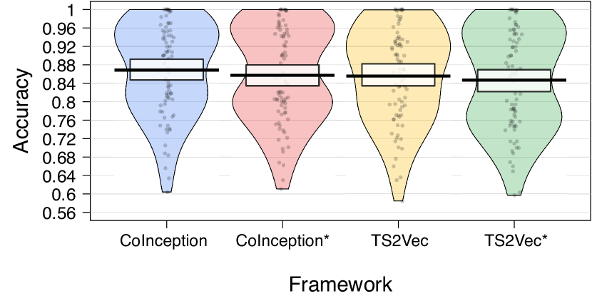
Figure 9: Transferability Analysis. Accuracy distribution for the first 85 UCR datasets.

Similarly, detailed results for the 30 UEA Repository datasets are summarized in Table 7, accompanied by the corresponding Critical Difference diagram for the first 29 datasets depicted in Figure 9. In line with the findings in the univariate setting, CoInception also achieves better performance than more than $55\%$ of the datasets in the UEA Repository’s multivariate scenario.

From both tables, it is evident that CoInception exhibits superior performance for the majority of datasets, resulting in a significant performance gap in terms of average accuracy.

Table 6: UCR 128 Datasets classification results. Best results are bold and highlighted in red.

Dataset	TS2Vec	T-Loss	TNC	TS-TCC	TST	DTW	CoInception	CoInception’s Rank
Adiac	0.762	0.675	0.726	0.767	0.550	0.604	0.767	1
ArrowHead	0.857	0.766	0.703	0.737	0.771	0.703	0.863	1
Beef	0.767	0.667	0.733	0.600	0.500	0.633	0.733	2
BeetleFly	0.900	0.800	0.850	0.800	1.000	0.700	0.850	3
BirdChicken	0.800	0.850	0.750	0.650	0.650	0.750	0.900	1
Car	0.833	0.833	0.683	0.583	0.550	0.733	0.867	1
CBF	1.000	0.983	0.983	0.998	0.898	0.997	1.000	1
ChlorineConcentration	0.832	0.749	0.760	0.753	0.562	0.648	0.813	2
CinCECGTorso	0.827	0.713	0.669	0.671	0.508	0.651	0.765	2
Coffee	1.000	1.000	1.000	1.000	0.821	1.000	1.000	1
Computers	0.660	0.664	0.684	0.704	0.696	0.700	0.688	4
CricketX	0.782	0.713	0.623	0.731	0.385	0.754	0.805	1
CricketY	0.749	0.728	0.597	0.718	0.467	0.744	0.818	1
CricketZ	0.792	0.708	0.682	0.713	0.403	0.754	0.808	1
DiatomSizeReduction	0.984	0.984	0.993	0.977	0.961	0.967	0.984	2
DistalPhalanxOutlineCorrect	0.761	0.775	0.754	0.754	0.728	0.717	0.779	1
DistalPhalanxOutlineAgeGroup	0.727	0.727	0.741	0.755	0.741	0.770	0.748	3
DistalPhalanxTW	0.698	0.676	0.669	0.676	0.568	0.590	0.705	1
Earthquakes	0.748	0.748	0.748	0.748	0.748	0.719	0.748	1
ECG200	0.920	0.940	0.830	0.880	0.830	0.770	0.920	2
ECG5000	0.935	0.933	0.937	0.941	0.928	0.924	0.944	1
ECGFiveDays	1.000	1.000	0.999	0.878	0.763	0.768	1.000	1
ElectricDevices	0.721	0.707	0.700	0.686	0.676	0.602	0.741	1
FaceAll	0.771	0.786	0.766	0.813	0.504	0.808	0.842	1
FaceFour	0.932	0.920	0.659	0.773	0.511	0.830	0.955	1
FacesUCR	0.924	0.884	0.789	0.863	0.543	0.905	0.928	1
FiftyWords	0.771	0.732	0.653	0.653	0.525	0.690	0.778	1
Fish	0.926	0.891	0.817	0.817	0.720	0.823	0.954	1
FordA	0.936	0.928	0.902	0.930	0.568	0.555	0.930	2
FordB	0.794	0.793	0.733	0.815	0.507	0.620	0.832	1
GunPoint	0.980	0.980	0.967	0.993	0.827	0.907	0.987	2
Ham	0.714	0.724	0.752	0.743	0.524	0.467	0.810	1
HandOutlines	0.922	0.922	0.930	0.724	0.735	0.881	0.935	1
Haptics	0.526	0.490	0.474	0.396	0.357	0.377	0.510	2
Herring	0.641	0.594	0.594	0.594	0.594	0.531	0.594	2
InlineSkate	0.415	0.371	0.378	0.347	0.287	0.384	0.424	1
InsectWingbeatSound	0.630	0.597	0.549	0.415	0.266	0.355	0.634	1
ItalyPowerDemand	0.925	0.954	0.928	0.955	0.845	0.950	0.962	1
LargeKitchenAppliances	0.845	0.789	0.776	0.848	0.595	0.795	0.893	1
Lightning2	0.869	0.869	0.869	0.836	0.705	0.869	0.902	1
Lightning7	0.863	0.795	0.767	0.685	0.411	0.726	0.836	2
Mallat	0.914	0.951	0.871	0.922	0.713	0.934	0.953	1
Meat	0.950	0.950	0.917	0.883	0.900	0.933	0.967	1
MedicalImages	0.789	0.750	0.754	0.747	0.632	0.737	0.795	1
MiddlePhalanxOutlineCorrect	0.838	0.825	0.818	0.818	0.753	0.698	0.832	2
MiddlePhalanxOutlineAgeGroup	0.636	0.656	0.643	0.630	0.617	0.500	0.656	1
MiddlePhalanxTW	0.584	0.591	0.571	0.610	0.506	0.506	0.604	2
MoteStrain	0.861	0.851	0.825	0.843	0.768	0.835	0.873	1
NonInvasiveFetalECGThorax1	0.930	0.878	0.898	0.898	0.471	0.790	0.919	2
NonInvasiveFetalECGThorax2	0.938	0.919	0.912	0.913	0.832	0.865	0.942	1
OliveOil	0.900	0.867	0.833	0.800	0.800	0.833	0.900	1
OSULeaf	0.851	0.760	0.723	0.723	0.545	0.591	0.835	2
PhalangesOutlinesCorrect	0.809	0.784	0.787	0.804	0.773	0.728	0.818	1
Phoneme	0.312	0.276	0.180	0.242	0.139	0.228	0.310	2
Plane	1.000	0.990	1.000	1.000	0.933	1.000	1.000	1
ProximalPhalanxOutlineCorrect	0.887	0.859	0.866	0.873	0.770	0.784	0.911	1
ProximalPhalanxOutlineAgeGroup	0.834	0.844	0.854	0.839	0.854	0.805	0.849	3
ProximalPhalanxTW	0.824	0.771	0.810	0.800	0.780	0.761	0.824	1
RefrigerationDevices	0.589	0.515	0.565	0.563	0.483	0.464	0.597	1
ScreenType	0.411	0.416	0.509	0.419	0.419	0.397	0.413	5
ShapeletSim	1.000	0.672	0.589	0.683	0.489	0.650	0.994	2
ShapesAll	0.902	0.848	0.788	0.773	0.733	0.768	0.898	2
SmallKitchenAppliances	0.731	0.677	0.725	0.691	0.592	0.643	0.792	1
SonyAIBORobotSurface1	0.903	0.902	0.804	0.899	0.724	0.725	0.908	1
SonyAIBORobotSurface2	0.871	0.889	0.834	0.907	0.745	0.831	0.939	1

Dataset	TS2Vec	T-Loss	TNC	TS-TCC	TST	DTW	CoInception	CoInception’s Rank
StarLightCurves	0.969	0.964	0.968	0.967	0.949	0.907	0.971	1
Strawberry	0.962	0.954	0.951	0.965	0.916	0.941	0.970	1
SwedishLeaf	0.941	0.914	0.880	0.923	0.738	0.792	0.950	1
Symbols	0.976	0.963	0.885	0.916	0.786	0.950	0.970	2
SyntheticControl	0.997	0.987	1.000	0.990	0.490	0.993	0.997	2
ToeSegmentation1	0.917	0.939	0.864	0.930	0.807	0.772	0.943	1
ToeSegmentation2	0.892	0.900	0.831	0.877	0.615	0.838	0.908	1
Trace	1.000	0.990	1.000	1.000	1.000	1.000	1.000	1
TwoLeadECG	0.986	0.999	0.993	0.976	0.871	0.905	0.998	2
TwoPatterns	1.000	0.999	1.000	0.999	0.466	1.000	1.000	1
UWaveGestureLibraryX	0.795	0.785	0.781	0.733	0.569	0.728	0.817	1
UWaveGestureLibraryY	0.719	0.710	0.697	0.641	0.348	0.634	0.739	1
UWaveGestureLibraryZ	0.770	0.757	0.721	0.690	0.655	0.658	0.771	1
UWaveGestureLibraryAll	0.930	0.896	0.903	0.692	0.475	0.892	0.937	1
Wafer	0.998	0.992	0.994	0.994	0.991	0.980	0.999	1
Wine	0.870	0.815	0.759	0.778	0.500	0.574	0.907	1
WordSynonyms	0.676	0.691	0.630	0.531	0.422	0.649	0.683	2
Worms	0.701	0.727	0.623	0.753	0.455	0.584	0.740	2
WormsTwoClass	0.805	0.792	0.727	0.753	0.584	0.623	0.818	1
Yoga	0.887	0.837	0.812	0.791	0.830	0.837	0.882	2
ACSF1	0.900	0.900	0.730	0.730	0.760	0.640	0.910	1
AllGestureWiimoteX	0.777	0.763	0.703	0.697	0.259	0.716	0.799	1
AllGestureWiimoteY	0.793	0.726	0.699	0.741	0.423	0.729	0.776	2
AllGestureWiimoteZ	0.746	0.723	0.646	0.689	0.447	0.643	0.747	1
BME	0.993	0.993	0.973	0.933	0.760	0.900	0.980	3
Chinatown	0.965	0.951	0.977	0.983	0.936	0.957	0.985	1
Crop	0.756	0.722	0.738	0.742	0.710	0.665	0.757	1
EOGHorizontalSignal	0.539	0.605	0.442	0.401	0.373	0.503	0.577	2
EOGVerticalSignal	0.503	0.434	0.392	0.376	0.298	0.448	0.564	1
EthanolLevel	0.468	0.382	0.424	0.486	0.260	0.276	0.496	1
FreezerRegularTrain	0.986	0.956	0.991	0.989	0.922	0.899	0.994	1
FreezerSmallTrain	0.870	0.933	0.982	0.979	0.920	0.753	0.919	5
Fungi	0.957	1.000	0.527	0.753	0.366	0.839	0.962	2
GestureMidAirD1	0.608	0.608	0.431	0.369	0.208	0.569	0.662	1
GestureMidAirD2	0.469	0.546	0.362	0.254	0.138	0.608	0.592	2
GestureMidAirD3	0.292	0.285	0.292	0.177	0.154	0.323	0.392	1
GesturePebbleZ1	0.930	0.919	0.378	0.395	0.500	0.791	0.872	3
GesturePebbleZ2	0.873	0.899	0.316	0.430	0.380	0.671	0.911	1
GunPointAgeSpan	0.987	0.994	0.984	0.994	0.991	0.918	1.000	1
GunPointMaleVersusFemale	1.000	0.997	0.994	0.997	1.000	0.997	1.000	1
GunPointOldVersusYoung	1.000	1.000	1.000	1.000	1.000	0.838	1.000	1
HouseTwenty	0.916	0.933	0.782	0.790	0.815	0.924	0.899	4
InsectEPGRegularTrain	1.000	1.000	1.000	1.000	1.000	0.872	1.000	1
InsectEPGSmallTrain	1.000	1.000	1.000	1.000	1.000	0.735	1.000	1
MelbournePedestrian	0.959	0.944	0.942	0.949	0.741	0.791	0.961	1
MixedShapesRegularTrain	0.917	0.905	0.911	0.855	0.879	0.842	0.933	1
MixedShapesSmallTrain	0.861	0.860	0.813	0.735	0.828	0.780	0.876	1
PickupGestureWiimoteZ	0.820	0.740	0.620	0.600	0.240	0.660	0.880	1
PigAirwayPressure	0.630	0.510	0.413	0.380	0.120	0.106	0.827	1
PigArtPressure	0.966	0.928	0.808	0.524	0.774	0.245	0.966	1
PigCVP	0.812	0.788	0.649	0.615	0.596	0.154	0.899	1
PLAID	0.561	0.555	0.495	0.445	0.419	0.840	0.533	4
PowerCons	0.961	0.900	0.933	0.961	0.911	0.878	0.983	1
Rock	0.700	0.580	0.580	0.600	0.680	0.600	0.660	3
SemgHandGenderCh2	0.963	0.890	0.882	0.837	0.725	0.802	0.962	2
SemgHandMovementCh2	0.860	0.789	0.593	0.613	0.420	0.584	0.811	2
SemgHandSubjectCh2	0.951	0.853	0.771	0.753	0.484	0.727	0.918	2
ShakeGestureWiimoteZ	0.940	0.920	0.820	0.860	0.760	0.860	0.920	2
SmoothSubspace	0.980	0.960	0.913	0.953	0.827	0.827	0.993	1
UMD	1.000	0.993	0.993	0.986	0.910	0.993	1.000	1
DodgerLoopDay	0.562	–	–	–	0.200	0.500	0.588	1
DodgerLoopGame	0.841	–	–	–	0.696	0.877	0.884	1
DodgerLoopWeekend	0.964	–	–	–	0.732	0.949	0.986	1
Avg. (first 125 datasets)	0.829	0.806	0.761	0.757	0.641	0.726	0.843	1.469

Table 7: UEA 30 Datasets classification results. Best results are bold and highlighted in red.

Dataset	TS2Vec	T-Loss	TNC	TS-TCC	TST	DTW	CoInception	Rank
ArticularyWordRecognition	0.987	0.943	0.973	0.953	0.977	0.987	0.987	1
AtrialFibrillation	0.200	0.133	0.133	0.267	0.067	0.200	0.333	1
BasicMotions	0.975	1.000	0.975	1.000	0.975	0.975	1.000	1
CharacterTrajectories	0.995	0.993	0.967	0.985	0.975	0.989	0.992	3
Cricket	0.972	0.972	0.958	0.917	1.000	1.000	0.986	3
DuckDuckGeese	0.680	0.650	0.460	0.380	0.620	0.600	0.500	5
EigenWorms	0.847	0.840	0.840	0.779	0.748	0.618	0.847	1
Epilepsy	0.964	0.971	0.957	0.957	0.949	0.964	0.978	1
ERing	0.874	0.133	0.852	0.904	0.874	0.133	0.900	2
EthanolConcentration	0.308	0.205	0.297	0.285	0.262	0.323	0.319	2
FaceDetection	0.501	0.513	0.536	0.544	0.534	0.529	0.550	1
FingerMovements	0.480	0.580	0.470	0.460	0.560	0.530	0.550	3
HandMovementDirection	0.338	0.351	0.324	0.243	0.243	0.231	0.351	1
Handwriting	0.515	0.451	0.249	0.498	0.225	0.286	0.549	1
Heartbeat	0.683	0.741	0.746	0.751	0.746	0.717	0.790	1
JapaneseVowels	0.984	0.989	0.978	0.930	0.978	0.949	0.992	1
Libras	0.867	0.883	0.817	0.822	0.656	0.870	0.867	3
LSST	0.537	0.509	0.595	0.474	0.408	0.551	0.537	3
MotorImagery	0.510	0.580	0.500	0.610	0.500	0.500	0.560	3
NATOPS	0.928	0.917	0.911	0.822	0.850	0.883	0.972	1
PEMS-SF	0.682	0.676	0.699	0.734	0.740	0.711	0.786	1
PenDigits	0.989	0.981	0.979	0.974	0.560	0.977	0.991	1
PhonemeSpectra	0.233	0.222	0.207	0.252	0.085	0.151	0.260	1
RacketSports	0.855	0.855	0.776	0.816	0.809	0.803	0.868	1
SelfRegulationSCP1	0.812	0.843	0.799	0.823	0.754	0.775	0.765	6
SelfRegulationSCP2	0.578	0.539	0.550	0.533	0.550	0.539	0.556	2
SpokenArabicDigits	0.988	0.905	0.934	0.970	0.923	0.963	0.979	2
StandWalkJump	0.467	0.333	0.400	0.333	0.267	0.200	0.533	1
UWaveGestureLibrary	0.906	0.875	0.759	0.753	0.575	0.903	0.894	3
InsectWingbeat	0.466	0.156	0.469	0.264	0.105	–	0.449	3
Avg. (first 29 datasets)	0.712	0.675	0.677	0.682	0.635	0.650	0.731	1

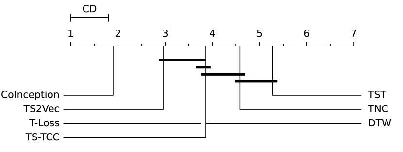
Figure 8: Critical Difference Diagram. Different classifiers’ ranks on 29 Datasets from UEA Repository with the confidence level of $95\%$.

Time Series Abnormally Detection

Additional details. In the preprocessing stage, we utilize the Augmented Dickey-Fuller (ADF) test, as done in [55, 65], to determine the number of unit roots, denoted as $d$. Subsequently, the data is differenced $d$ times to mitigate any drifting effect, following the approach described in [65].

For the evaluation process, we adopt a similar protocol as presented in [65, 44, 63], aimed at relaxing the point-wise detection constraint. Within this protocol, a small delay is allowed after the appearance of each anomaly point. Specifically, for minutely data, a maximum delay of $7$ steps is accepted, while for hourly data, a delay of $3$ steps is employed. If the detector correctly identifies the point within this delay, all points within the corresponding segment are considered correct; otherwise, they are deemed incorrect.

Receptive Field Analysis

This experiment aims to investigate the scalability of the CoInception framework in comparison to the stacked Dilated Convolution network proposed in [65]. We present a visualization of the relationship between the network depth, the number of parameters, and the maximum receptive fields of output timestamps in Figure 10.

The receptive field represents the number of input timestamps involved in calculating an output timestamp. The reported statistics for both the number of parameters and the receptive field are presented in logarithmic scale to ensure smoothness and a smaller number range.

As depicted in the figure, CoInception consistently exhibits a lower number of parameters compared to TS2Vec, across a network depth ranging from 1 to 30 layers. It is worth noting that the inclusion of a 30-layer CoInception framework in the visualization is purely for illustrative purposes, as we believe a much smaller depth is sufficient for the majority of time series datasets. In fact, we only utilize 3 layers for all datasets in the remaining sections. Furthermore, CoInception, with its multiple Basic units of varying filter lengths, can easily achieve very large receptive fields even with just a few layers.

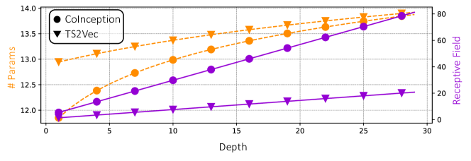
Figure 10: Receptive Field Analysis. The relation between models’ depth with their number of parameters and their maximum receptive field.

Clusterability Analysis

Through this experiment, we test the clusterability of the learnt representations in the latent space. We visualize the feature representations with t-SNE proposed by Maaten and partners - [58] in two dimensional space. In the best scenario, the representations should be presented in latent space by groups of clusters, basing on their labels - their underlying states.

Figure 11 compares the distribution of representations learned by CoInception and TS2Vec in three dataset with greatest test set in UCR 128 repository. It is evident that the proposed CoInception does outperform the second best TS2Vec in terms of representation learning from the same hidden state. The clusters learnt by CoInception are more compact than those produced by TS2Vec, especially when the number of classes increase for ElectricDevices or Crop datasets.

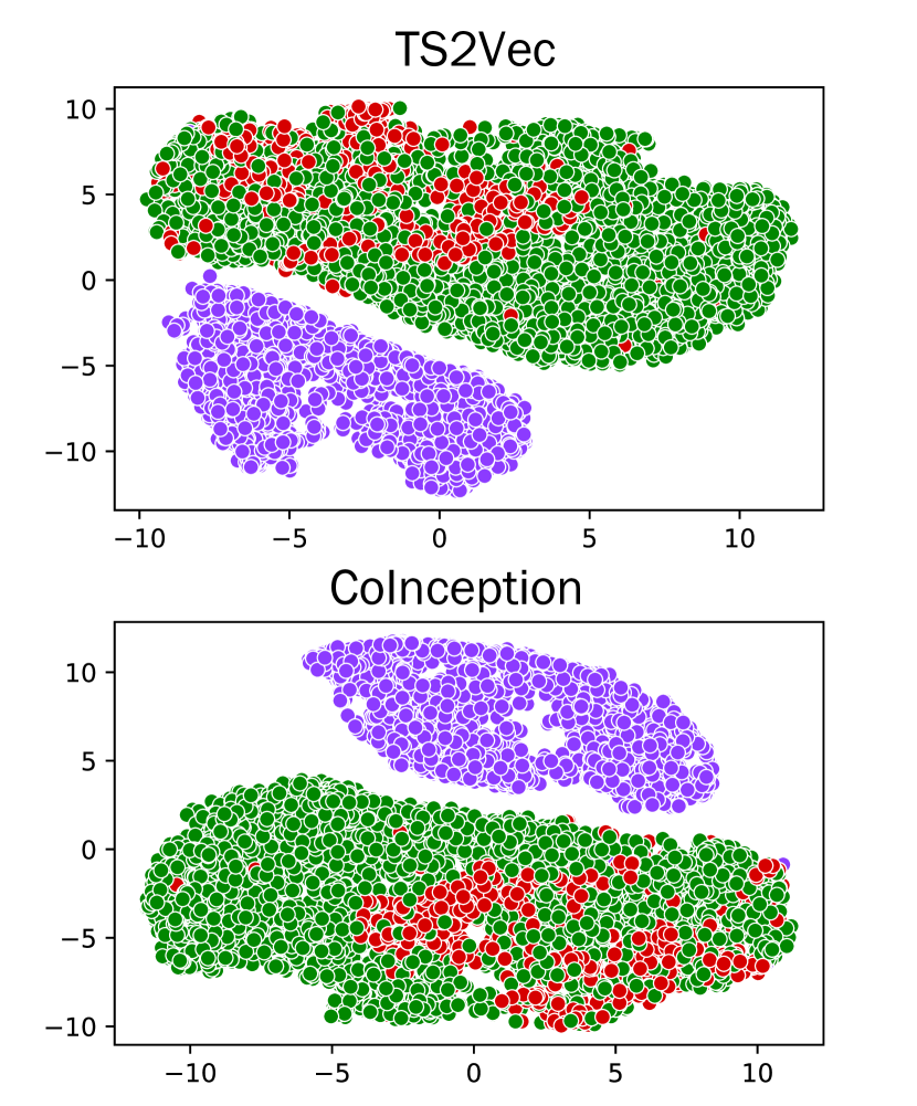
(a) StarLightCurves

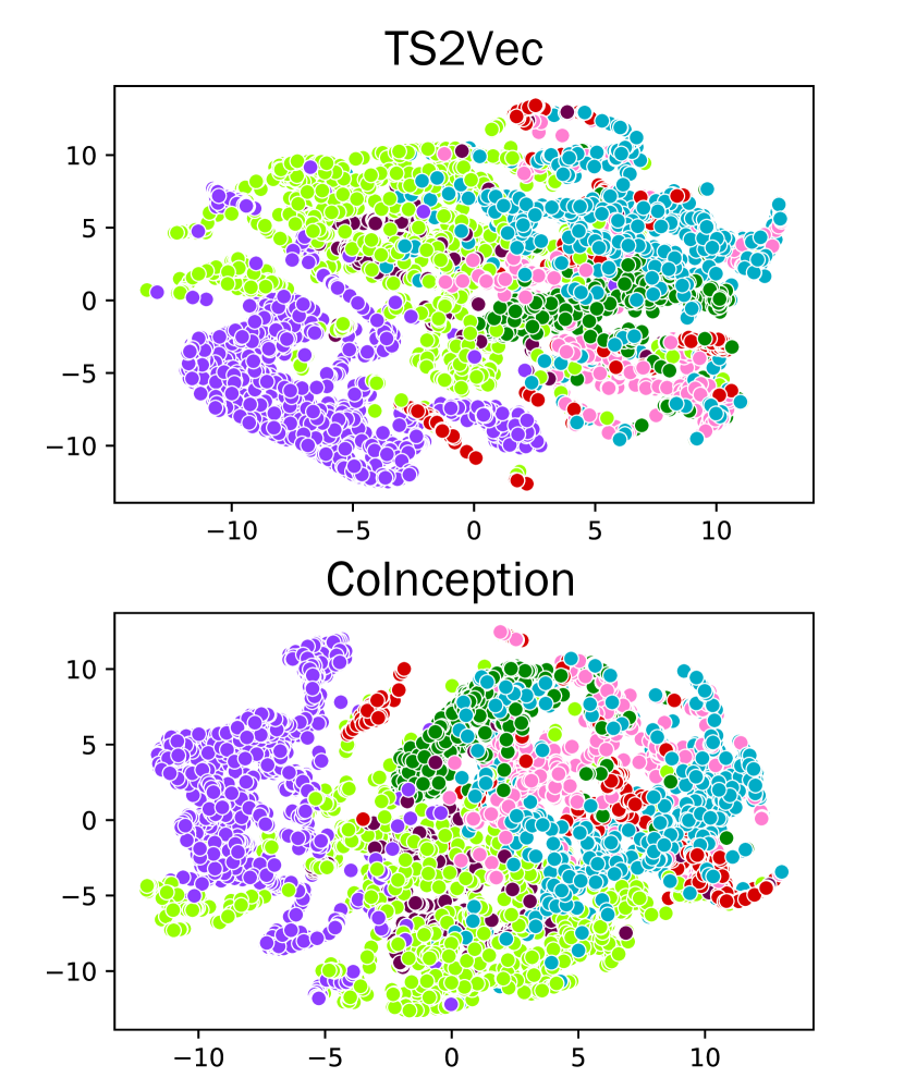
(b) ElectricDevices

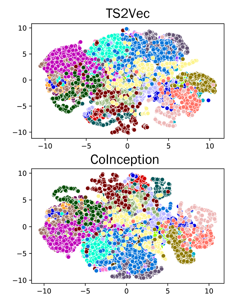
(c) Crop

Figure 11: Comparing clusterability of our CoInception with TS2Vec over three benchmark datasets in UCR 125 Repository.

Transferability Analysis

We assess the transferability of CoInception framework under all three tasks: forecasting, classification and anomaly detection.

For the forecasting task, we evaluate the transferability of the CoInception framework using the following approach. The ETT datasets [69] consist of power transformer data collected from July 2016 to July 2018. We focus on the small datasets, which include data from 2 stations, specifically load and oil temperature. ETTh1 and ETTh2 are datasets with a temporal granularity of 1 hour, corresponding to the two stations. Since these two datasets exhibit high correlation, we leverage transfer learning between them. Initially, we perform the unsupervised learning step on the ETTh1 dataset, similar to the process used for forecasting assessment. Subsequently, the weights of the CoInception Encoder are frozen, and we utilize this pre-trained Encoder for training the forecasting framework, employing a Ridge Regression model, on the ETTh2 dataset.

Table 8: Transferability analysis with time series forecasting task.

	Forecasting (ETTh1 ->ETTh2)
Model	24 Step	48 Step	168 Step	336 Step	720 Step
TS2Vec	0.090	0.124	0.208	0.213	0.214
TS2Vec*	0.100	0.143	0.236	0.223	0.217
CoInception	0.086	0.119	0.185	0.196	0.209
CoInception*	0.084	0.118	0.188	0.201	0.211

The detailed results are presented in Table 8. Overall, CoInception demonstrates its strong adaptability to the ETTh2 dataset, surpassing TS2Vec and even performing comparably to its own results in the regular forecasting setting.

For classification task, we follow the settings in [18]. We first train our Encoder unsupervisedly with training data from FordA dataset. Following, for each dataset in UCR repository, the SVM classifier is trained on top of the representations produced by the frozen CoInception Encoder with this dataset. Table 9 provides a summary of the transferability results on the first 85 UCR datasets. Although CoInception exhibits lower performance compared to its own results in the regular classification setting in most datasets, its overall performance, as measured by the average accuracy, is still comparable to TS2Vec in its normal settings.

For anomaly detection, the settings are inherited from [44, 65], and we have already presented the results with cold-start settings in the main manuscript.

Table 9: Transferability analysis for time series classification.

Dataset	TS2Vec	TS2Vec∗	T-Loss	T-Loss∗	CoInception	CoInception∗
Adiac	0.762	0.783	0.760	0.716	0.767	0.803
ArrowHead	0.857	0.829	0.817	0.829	0.863	0.806
Beef	0.767	0.700	0.667	0.700	0.733	0.733
BeetleFly	0.900	0.900	0.800	0.900	0.850	0.900
BirdChicken	0.800	0.800	0.900	0.800	0.900	0.800
Car	0.833	0.817	0.850	0.817	0.867	0.883
CBF	1.000	1.000	0.988	0.994	1.000	0.997
ChlorineConcentration	0.832	0.802	0.688	0.782	0.813	0.814
CinCECGTorso	0.827	0.738	0.638	0.740	0.765	0.772
Coffee	1.000	1.000	1.000	1.000	1.000	1.000
Computers	0.660	0.660	0.648	0.628	0.688	0.668
CricketX	0.782	0.767	0.682	0.777	0.805	0.767
CricketY	0.749	0.746	0.667	0.767	0.818	0.751
CricketZ	0.792	0.772	0.656	0.764	0.808	0.762
DiatomSizeReduction	0.984	0.961	0.974	0.993	0.984	0.977
DistalPhalanxOutlineCorrect	0.761	0.757	0.764	0.768	0.779	0.775
DistalPhalanxOutlineAgeGroup	0.727	0.748	0.727	0.734	0.748	0.741
DistalPhalanxTW	0.698	0.669	0.669	0.676	0.705	0.698
Earthquakes	0.748	0.748	0.748	0.748	0.748	0.748
ECG200	0.920	0.910	0.830	0.900	0.920	0.920
ECG5000	0.935	0.935	0.940	0.936	0.944	0.942
ECGFiveDays	1.000	1.000	1.000	1.000	1.000	1.000
ElectricDevices	0.721	0.714	0.676	0.732	0.741	0.722
FaceAll	0.771	0.786	0.734	0.802	0.842	0.821
FaceFour	0.932	0.898	0.830	0.875	0.955	0.807
FacesUCR	0.924	0.928	0.835	0.918	0.928	0.923
FiftyWords	0.771	0.785	0.745	0.780	0.778	0.804
Fish	0.926	0.949	0.960	0.880	0.954	0.943
FordA	0.936	0.936	0.927	0.935	0.930	0.943
FordB	0.794	0.779	0.798	0.810	0.802	0.796
GunPoint	0.980	0.993	0.987	0.993	0.987	0.987
Ham	0.714	0.714	0.533	0.695	0.810	0.648
HandOutlines	0.922	0.919	0.919	0.922	0.935	0.930
Haptics	0.526	0.526	0.474	0.455	0.510	0.513
Herring	0.641	0.594	0.578	0.578	0.594	0.609
InlineSkate	0.415	0.465	0.444	0.447	0.424	0.453
InsectWingbeatSound	0.630	0.603	0.599	0.623	0.634	0.630
ItalyPowerDemand	0.925	0.957	0.929	0.925	0.962	0.963
LargeKitchenAppliances	0.845	0.861	0.765	0.848	0.893	0.787
Lightning2	0.869	0.918	0.787	0.918	0.902	0.852
Lightning7	0.863	0.781	0.740	0.795	0.836	0.808
Mallat	0.914	0.956	0.916	0.964	0.953	0.966
Meat	0.950	0.967	0.867	0.950	0.967	0.967
MedicalImages	0.789	0.784	0.725	0.784	0.795	0.792
MiddlePhalanxOutlineCorrect	0.838	0.794	0.787	0.814	0.832	0.838
MiddlePhalanxOutlineAgeGroup	0.636	0.649	0.623	0.656	0.656	0.662
MiddlePhalanxTW	0.584	0.597	0.584	0.610	0.604	0.610
MoteStrain	0.861	0.847	0.823	0.871	0.873	0.822
NonInvasiveFetalECGThorax1	0.930	0.946	0.925	0.910	0.919	0.947
NonInvasiveFetalECGThorax2	0.938	0.955	0.930	0.927	0.942	0.950
OliveOil	0.900	0.900	0.900	0.900	0.900	0.900
OSULeaf	0.851	0.868	0.736	0.831	0.835	0.777
PhalangesOutlinesCorrect	0.809	0.794	0.784	0.801	0.818	0.800
Phoneme	0.312	0.260	0.196	0.289	0.310	0.294

Dataset	TS2Vec	TS2Vec∗	T-Loss	T-Loss∗	CoInception	CoInception∗
Plane	1.000	0.981	0.981	0.990	1.000	1.000
ProximalPhalanxOutlineCorrect	0.887	0.876	0.869	0.859	0.911	0.893
ProximalPhalanxOutlineAgeGroup	0.834	0.844	0.839	0.854	0.849	0.844
ProximalPhalanxTW	0.824	0.805	0.785	0.824	0.824	0.820
RefrigerationDevices	0.589	0.557	0.555	0.517	0.597	0.635
ScreenType	0.411	0.421	0.384	0.413	0.413	0.469
ShapeletSim	1.000	1.000	0.517	0.817	0.994	1.000
ShapesAll	0.902	0.877	0.837	0.875	0.898	0.863
SmallKitchenAppliances	0.731	0.747	0.731	0.715	0.792	0.717
SonyAIBORobotSurface1	0.903	0.884	0.840	0.897	0.908	0.903
SonyAIBORobotSurface2	0.871	0.872	0.832	0.934	0.939	0.940
StarLightCurves	0.969	0.967	0.968	0.965	0.971	0.974
Strawberry	0.962	0.962	0.946	0.946	0.970	0.970
SwedishLeaf	0.941	0.931	0.925	0.931	0.950	0.957
Symbols	0.976	0.973	0.945	0.965	0.970	0.961
SyntheticControl	0.997	0.997	0.977	0.983	0.997	0.990
ToeSegmentation1	0.917	0.947	0.899	0.952	0.943	0.947
ToeSegmentation2	0.892	0.946	0.900	0.885	0.908	0.900
Trace	1.000	1.000	1.000	1.000	1.000	1.000
TwoLeadECG	0.986	0.999	0.993	0.997	0.998	0.999
TwoPatterns	1.000	0.999	0.992	1.000	1.000	1.000
UWaveGestureLibraryX	0.795	0.818	0.784	0.811	0.817	0.820
UWaveGestureLibraryY	0.719	0.739	0.697	0.735	0.739	0.738
UWaveGestureLibraryZ	0.770	0.757	0.729	0.759	0.771	0.754
UWaveGestureLibraryAll	0.930	0.918	0.865	0.941	0.937	0.956
Wafer	0.998	0.997	0.995	0.993	0.999	0.998
Wine	0.870	0.759	0.685	0.870	0.907	0.907
WordSynonyms	0.676	0.693	0.641	0.704	0.683	0.691
Worms	0.701	0.753	0.688	0.714	0.740	0.701
WormsTwoClass	0.805	0.688	0.753	0.818	0.818	0.779
Yoga	0.887	0.855	0.828	0.878	0.882	0.854
Avg. (first 85 datasets)	0.829	0.824	0.786	0.821	0.841	0.829

References

- [1] Arthur Asuncion and David Newman. Uci machine learning repository, 2007.
- [2] Anthony Bagnall, Hoang Anh Dau, Jason Lines, Michael Flynn, James Large, Aaron Bostrom, Paul Southam, and Eamonn Keogh. The uea multivariate time series classification archive, 2018. arXiv preprint arXiv:1811.00075, 2018.
- [3] Shaojie Bai, J Zico Kolter, and Vladlen Koltun. An empirical evaluation of generic convolutional and recurrent networks for sequence modeling. arXiv preprint arXiv:1803.01271, 2018.
- [4] George EP Box, Gwilym M Jenkins, Gregory C Reinsel, and Greta M Ljung. Time series analysis: forecasting and control. John Wiley & Sons, 2015.
- [5] Defu Cao, Yujing Wang, Juanyong Duan, Ce Zhang, Xia Zhu, Congrui Huang, Yunhai Tong, Bixiong Xu, Jing Bai, Jie Tong, et al. Spectral temporal graph neural network for multivariate time-series forecasting. Advances in neural information processing systems, 33:17766–17778, 2020.
- [6] Mathilde Caron, Piotr Bojanowski, Armand Joulin, and Matthijs Douze. Deep clustering for unsupervised learning of visual features. In Proceedings of the European conference on computer vision (ECCV), pages 132–149, 2018.
- [7] Gal Chechik, Varun Sharma, Uri Shalit, and Samy Bengio. Large scale online learning of image similarity through ranking. Journal of Machine Learning Research, 11(3), 2010.
- [8] Yahui Chen. Convolutional neural network for sentence classification. Master’s thesis, University of Waterloo, 2015.
- [9] Yanping Chen, Bing Hu, Eamonn Keogh, and Gustavo EAPA Batista. Dtw-d: time series semi-supervised learning from a single example. In Proceedings of the 19th ACM SIGKDD international conference on Knowledge discovery and data mining, pages 383–391, 2013.
- [10] Edward Choi, Mohammad Taha Bahadori, Elizabeth Searles, Catherine Coffey, Michael Thompson, James Bost, Javier Tejedor-Sojo, and Jimeng Sun. Multi-layer representation learning for medical concepts. In proceedings of the 22nd ACM SIGKDD international conference on knowledge discovery and data mining, pages 1495–1504, 2016.
- [11] Hoang Anh Dau, Anthony Bagnall, Kaveh Kamgar, Chin-Chia Michael Yeh, Yan Zhu, Shaghayegh Gharghabi, Chotirat Ann Ratanamahatana, and Eamonn Keogh. The ucr time series archive. IEEE/CAA Journal of Automatica Sinica, 6(6):1293–1305, 2019.
- [12] Ingrid Daubechies. The wavelet transform, time-frequency localization and signal analysis. IEEE transactions on information theory, 36(5):961–1005, 1990.
- [13] Ingrid Daubechies. Ten lectures on wavelets. SIAM, 1992.
- [14] Janez Demšar. Statistical comparisons of classifiers over multiple data sets. The Journal of Machine learning research, 7:1–30, 2006.
- [15] Ch Dolabdjian, J Fadili, and E Huertas Leyva. Classical low-pass filter and real-time wavelet-based denoising technique implemented on a dsp: a comparison study. The European Physical Journal-Applied Physics, 20(2):135–140, 2002.
- [16] Yihe Dong, Jean-Baptiste Cordonnier, and Andreas Loukas. Attention is not all you need: Pure attention loses rank doubly exponentially with depth. In International Conference on Machine Learning, pages 2793–2803. PMLR, 2021.
- [17] Emadeldeen Eldele, Mohamed Ragab, Zhenghua Chen, Min Wu, C. Kwoh, Xiaoli Li, and Cuntai Guan. Time-series representation learning via temporal and contextual contrasting. ArXiv, abs/2106.14112, 2021.
- [18] Jean-Yves Franceschi, Aymeric Dieuleveut, and Martin Jaggi. Unsupervised scalable representation learning for multivariate time series. Advances in neural information processing systems, 32, 2019.
- [19] Priyanka Gupta, Pankaj Malhotra, Lovekesh Vig, and Gautam Shroff. Transfer learning for clinical time series analysis using recurrent neural networks. arXiv preprint arXiv:1807.01705, 2018.
- [20] Elad Hoffer and Nir Ailon. Deep metric learning using triplet network. In Similarity-Based Pattern Recognition: Third International Workshop, SIMBAD 2015, Copenhagen, Denmark, October 12-14, 2015. Proceedings 3, pages 84–92. Springer, 2015.
- [21] Md Amirul Islam, Sen Jia, and Neil DB Bruce. How much position information do convolutional neural networks encode? arXiv preprint arXiv:2001.08248, 2020.
- [22] Hassan Ismail Fawaz, Benjamin Lucas, Germain Forestier, Charlotte Pelletier, Daniel F Schmidt, Jonathan Weber, Geoffrey I Webb, Lhassane Idoumghar, Pierre-Alain Muller, and François Petitjean. Inceptiontime: Finding alexnet for time series classification. Data Mining and Knowledge Discovery, 34(6):1936–1962, 2020.
- [23] Armand Joulin, Edouard Grave, Piotr Bojanowski, and Tomas Mikolov. Bag of tricks for efficient text classification. arXiv preprint arXiv:1607.01759, 2016.
- [24] Mehmet Kayaalp. Patient privacy in the era of big data. Balkan medical journal, 35(1):8–17, 2018.
- [25] Nikita Kitaev, Łukasz Kaiser, and Anselm Levskaya. Reformer: The efficient transformer. arXiv preprint arXiv:2001.04451, 2020.
- [26] Dani Kiyasseh, Tingting Zhu, and David A Clifton. Clocs: Contrastive learning of cardiac signals across space, time, and patients. In International Conference on Machine Learning, pages 5606–5615. PMLR, 2021.
- [27] Guokun Lai, Wei-Cheng Chang, Yiming Yang, and Hanxiao Liu. Modeling long-and short-term temporal patterns with deep neural networks. In The 41st international ACM SIGIR conference on research & development in information retrieval, pages 95–104, 2018.
- [28] T Lanting, MHS Amin, MW Johnson, F Altomare, AJ Berkley, S Gildert, R Harris, J Johansson, P Bunyk, E Ladizinsky, et al. Probing high-frequency noise with macroscopic resonant tunneling. Physical Review B, 83(18):180502, 2011.
- [29] Nikolay Laptev, Saeed Amizadeh, and Youssef Billawala. A benchmark dataset for time series anomaly detection, 2015.
- [30] Shiyang Li, Xiaoyong Jin, Yao Xuan, Xiyou Zhou, Wenhu Chen, Yu-Xiang Wang, and Xifeng Yan. Enhancing the locality and breaking the memory bottleneck of transformer on time series forecasting. Advances in neural information processing systems, 32, 2019.
- [31] Shiyang Li, Xiaoyong Jin, Yao Xuan, Xiyou Zhou, Wenhu Chen, Yu-Xiang Wang, and Xifeng Yan. Enhancing the locality and breaking the memory bottleneck of transformer on time series forecasting. Advances in neural information processing systems, 32, 2019.
- [32] Luminol. linkedin luminol. https://github.com/linkedin/luminol. Accessed: 2023-04-11.
- [33] Xinrui Lyu, Matthias Hueser, Stephanie L Hyland, George Zerveas, and Gunnar Raetsch. Improving clinical predictions through unsupervised time series representation learning. arXiv preprint arXiv:1812.00490, 2018.
- [34] Stéphane Mallat. A wavelet tour of signal processing. Elsevier, 1999.
- [35] Tomas Mikolov, Ilya Sutskever, Kai Chen, Greg S Corrado, and Jeff Dean. Distributed representations of words and phrases and their compositionality. Advances in neural information processing systems, 26, 2013.
- [36] Antonio Mucherino, Petraq Papajorgji, and Panos M Pardalos. A survey of data mining techniques applied to agriculture. Operational Research, 9:121–140, 2009.
- [37] Tsutomu Oohashi, Emi Nishina, Manabu Honda, Yoshiharu Yonekura, Yoshitaka Fuwamoto, Norie Kawai, Tadao Maekawa, Satoshi Nakamura, Hidenao Fukuyama, and Hiroshi Shibasaki. Inaudible high-frequency sounds affect brain activity: hypersonic effect. Journal of neurophysiology, 2000.
- [38] Boris N Oreshkin, Dmitri Carpov, Nicolas Chapados, and Yoshua Bengio. N-beats: Neural basis expansion analysis for interpretable time series forecasting. arXiv preprint arXiv:1905.10437, 2019.
- [39] Marcello Pagano. Estimation of models of autoregressive signal plus white noise. The annals of Statistics, pages 99–108, 1974.
- [40] Emanuel Parzen. Time series analysis for models of signal plus white noise. Technical report, STANFORD UNIV CALIF DEPT OF STATISTICS, 1966.
- [41] Deepak Pathak, Philipp Krahenbuhl, Jeff Donahue, Trevor Darrell, and Alexei A Efros. Context encoders: Feature learning by inpainting. In Proceedings of the IEEE conference on computer vision and pattern recognition, pages 2536–2544, 2016.
- [42] C-K Peng, Shlomo Havlin, H Eugene Stanley, and Ary L Goldberger. Quantification of scaling exponents and crossover phenomena in nonstationary heartbeat time series. Chaos: an interdisciplinary journal of nonlinear science, 5(1):82–87, 1995.
- [43] Faraz Rasheed, Peter Peng, Reda Alhajj, and Jon Rokne. Fourier transform based spatial outlier mining. In Intelligent Data Engineering and Automated Learning-IDEAL 2009: 10th International Conference, Burgos, Spain, September 23-26, 2009. Proceedings 10, pages 317–324. Springer, 2009.
- [44] Hansheng Ren, Bixiong Xu, Yujing Wang, Chao Yi, Congrui Huang, Xiaoyu Kou, Tony Xing, Mao Yang, Jie Tong, and Qi Zhang. Time-series anomaly detection service at microsoft. In Proceedings of the 25th ACM SIGKDD international conference on knowledge discovery & data mining, pages 3009–3017, 2019.
- [45] Robert H Shumway, David S Stoffer, and David S Stoffer. Time series analysis and its applications, volume 3. Springer, 2000.
- [46] Ravid Shwartz-Ziv and Amitai Armon. Tabular data: Deep learning is not all you need. Information Fusion, 81:84–90, 2022.
- [47] Alban Siffer, Pierre-Alain Fouque, Alexandre Termier, and Christine Largouet. Anomaly detection in streams with extreme value theory. In Proceedings of the 23rd ACM SIGKDD International Conference on Knowledge Discovery and Data Mining, pages 1067–1075, 2017.
- [48] Athanassios Skodras. Discrete wavelet transform: An introduction, 12 2015.
- [49] Michael Small. Applied nonlinear time series analysis: applications in physics, physiology and finance, volume 52. World Scientific, 2005.
- [50] Xiaomin Song, Qingsong Wen, Yan Li, and Liang Sun. Robust time series dissimilarity measure for outlier detection and periodicity detection. In Proceedings of the 31st ACM International Conference on Information & Knowledge Management, pages 4510–4514, 2022.
- [51] Chen Sun, Abhinav Shrivastava, Saurabh Singh, and Abhinav Gupta. Revisiting unreasonable effectiveness of data in deep learning era. In Proceedings of the IEEE international conference on computer vision, pages 843–852, 2017.
- [52] Christian Szegedy, Vincent Vanhoucke, Sergey Ioffe, Jon Shlens, and Zbigniew Wojna. Rethinking the inception architecture for computer vision. In Proceedings of the IEEE conference on computer vision and pattern recognition, pages 2818–2826, 2016.
- [53] Van-Dai Ta, Chuan-Ming Liu, and Goodwill Wandile Nkabinde. Big data stream computing in healthcare real-time analytics. In 2016 IEEE international conference on cloud computing and big data analysis (ICCCBDA), pages 37–42. IEEE, 2016.
- [54] Chi Ian Tang, Ignacio Perez-Pozuelo, Dimitris Spathis, and Cecilia Mascolo. Exploring contrastive learning in human activity recognition for healthcare. arXiv preprint arXiv:2011.11542, 2020.
- [55] Sana Tonekaboni, Danny Eytan, and Anna Goldenberg. Unsupervised representation learning for time series with temporal neighborhood coding. In International Conference on Learning Representations, 2021.
- [56] Parishwad P Vaidyanathan. Multirate systems and filter banks. Pearson Education India, 2006.
- [57] Owen Vallis, Jordan Hochenbaum, and Arun Kejariwal. A novel technique for long-term anomaly detection in the cloud. In 6th USENIX workshop on hot topics in cloud computing (HotCloud 14), 2014.
- [58] Laurens van der Maaten and Geoffrey Hinton. Visualizing data using t-sne. Journal of Machine Learning Research, 9(86):2579–2605, 2008.
- [59] Renzhuo Wan, Shuping Mei, Jun Wang, Min Liu, and Fan Yang. Multivariate temporal convolutional network: A deep neural networks approach for multivariate time series forecasting. Electronics, 8(8):876, 2019.
- [60] Alex Wang, Amanpreet Singh, Julian Michael, Felix Hill, Omer Levy, and Samuel R Bowman. Glue: A multi-task benchmark and analysis platform for natural language understanding. arXiv preprint arXiv:1804.07461, 2018.
- [61] Tongzhou Wang and Phillip Isola. Understanding contrastive representation learning through alignment and uniformity on the hypersphere. In International Conference on Machine Learning, pages 9929–9939. PMLR, 2020.
- [62] Qingsong Wen, Jingkun Gao, Xiaomin Song, Liang Sun, Huan Xu, and Shenghuo Zhu. Robuststl: A robust seasonal-trend decomposition algorithm for long time series. In Proceedings of the AAAI Conference on Artificial Intelligence, volume 33, pages 5409–5416, 2019.
- [63] Haowen Xu, Wenxiao Chen, Nengwen Zhao, Zeyan Li, Jiahao Bu, Zhihan Li, Ying Liu, Youjian Zhao, Dan Pei, Yang Feng, et al. Unsupervised anomaly detection via variational auto-encoder for seasonal kpis in web applications. In Proceedings of the 2018 world wide web conference, pages 187–196, 2018.
- [64] Ling Yang and linda Qiao. Unsupervised time-series representation learning with iterative bilinear temporal-spectral fusion. In International Conference on Machine Learning, 2022.
- [65] Zhihan Yue, Yujing Wang, Juanyong Duan, Tianmeng Yang, Congrui Huang, Yunhai Tong, and Bixiong Xu. Ts2vec: Towards universal representation of time series. In Proceedings of the AAAI Conference on Artificial Intelligence, volume 36, pages 8980–8987, 2022.
- [66] George Zerveas, Srideepika Jayaraman, Dhaval Patel, Anuradha Bhamidipaty, and Carsten Eickhoff. A transformer-based framework for multivariate time series representation learning. In Proceedings of the 27th ACM SIGKDD Conference on Knowledge Discovery & Data Mining, pages 2114–2124, 2021.
- [67] Richard Zhang, Phillip Isola, and Alexei A Efros. Colorful image colorization. In Computer Vision–ECCV 2016: 14th European Conference, Amsterdam, The Netherlands, October 11-14, 2016, Proceedings, Part III 14, pages 649–666. Springer, 2016.
- [68] Xiang Zhang, Ziyuan Zhao, Theodoros Tsiligkaridis, and Marinka Zitnik. Self-supervised contrastive pre-training for time series via time-frequency consistency. arXiv preprint arXiv:2206.08496, 2022.
- [69] Haoyi Zhou, Shanghang Zhang, Jieqi Peng, Shuai Zhang, Jianxin Li, Hui Xiong, and Wancai Zhang. Informer: Beyond efficient transformer for long sequence time-series forecasting. Proceedings of the AAAI Conference on Artificial Intelligence, 35(12):11106–11115, May 2021.