AMEE: A Robust Framework for Explanation Evaluation in Time Series Classification

Abstract

Time series classification is a task which deals with a prevalent data type, temporal sequences, common in domains such as human activity recognition, sports analytics and general healthcare. This paper provides a framework to quantitatively evaluate and rank explanation methods for time series classification. The recent interest in explanation methods for time series has provided a great variety of explanation techniques. Nevertheless, when the explanations disagree on a specific problem, it remains unclear which of them to use. Comparing multiple explanations to find the right answer is non-trivial. Two key challenges remain: how to quantitatively and robustly evaluate the informativeness of a given explanation method (i.e., relevance for the classification task), and how to compare explanation methods side-by-side. We propose AMEE, a robust Model-Agnostic Explanation Evaluation framework for evaluating and comparing multiple saliency-based explanations for time series classification. In this approach, data perturbation is added to the input time series guided by each explanation. The impact of perturbation on classification accuracy is then measured and used for explanation evaluation. The results show that perturbing discriminative parts of the time series leads to significant changes in classification accuracy which can be used to evaluate each explanation. To be robust to different types of perturbations and different types of classifiers, we aggregate the accuracy loss across perturbations and classifiers. This novel approach allows us to quantify and rank different explanation methods. We provide a quantitative and qualitative analysis for synthetic datasets, a variety of time-series datasets, as well as a real-world dataset with known expert ground truth.

1 Introduction

The last decade witnessed a rapid integration and significant impact of machine learning in everyday life. Current machine learning algorithms work well in many applications and grow ever more complex with models having millions of parameters [11, 5]. However, we are far behind in explaining why these algorithms often work so well and occasionally fail to perform well [14]. While we have a whole range of new explanation methods and methodologies, it is still difficult to decide which explanation methods to select for a given problem and dataset.

This unmatched growth of complexity and explainability of many machine learning algorithms, including those dealing with time series data, undermines application of these technologies in critical, human-related areas such as medicine, healthcare, and finance [6, 25]. As time series data is prevalent in these applications [30, 31, 3], Time Series Classification (TSC) algorithms often call for reliable explanations [4, 20]. This explanation is usually presented in the form of feature importance or as a saliency map [1], highlighting the parts of the time series which are informative for the classification decision.

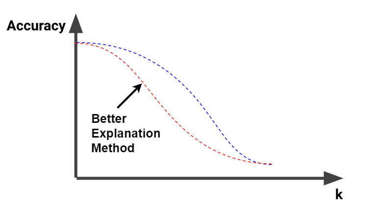
Figure 1: Changes of accuracy measured by a Referee classifier among two explanation methods (red and blue) at each threshold level $k$ . When a signal is perturbed based on a more informative explanation, this signal becomes harder for the referee to predict its class correctly, leading to a more severe drop in accuracy. This impact is measured by the Explanation AUC, or the the area under the curve (AUC) of these changes in accuracy at different threshold $k$. The curve with lower explanation AUC (red curve) results from perturbation from a more informative explanation method.

Recent efforts both in designing intrinsically explainable machine learning algorithms, as well as building post-hoc methods explaining black-box algorithms, have gained significant attention [40, 35, 32, 36, 26]; yet, these efforts present us with a new challenge: How to assess and objectively compare such methods? In other words, if two or more explanation techniques give different explanations (i.e., two different saliency maps, Figure 1), which technique and explanation should we use and trust?

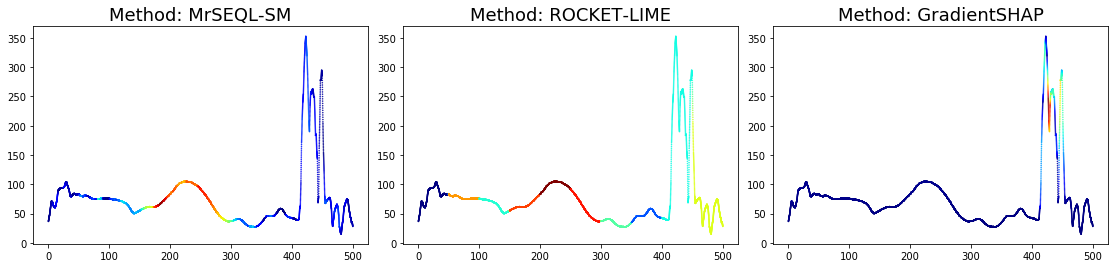
Figure 1: Saliency map explanations for classifying a motion time series obtained using different explanation methods. The most discriminative parts (according to the method) are colored in deep red and the most non-discriminative parts are colored in deep blue.

Our solution to this problem is a robust methodology resulting in a standardized metric, enabling quantitative comparison of explanation methods (Table 1). From the application users’ perspective, having this assessment can help reduce the need for expert feedback and support short-listing of useful explanations for user-studies which are generally costly and difficult to reproduce [12].

	Explanation Power [0-1]	Method Ranking [1-5]
Oracle	1.00	1(best)
MrSEQL-SM	0.90	2
ROCKET-LIME	0.56	3
ResNet-GradSHAP	0.06	4
Random	0.00	5 (worst)

Table 1: Outcome of AMEE: a measure to evaluate multiple explanation methods. Explanation Power measures the informativeness of each explanation method, taking values from 0 to 1, where 0 is worst and 1 is best.

In this paper, we present A Model-agnostic framework for Explanation Evaluation for Time Series Classification (AMEE). Specifically, we focus on explanation in the form of a saliency map and consider its informativeness within a defined computational scope, in which a more informative explanation means a higher capability to influence classifiers to correctly identify a class. Perturbation of discriminative subsequences of the time series results in a reduced accuracy of classifiers. The higher the impact of a perturbation means the more informative are the perturbed time series subsequences. Estimation of this impact, measured by a committee of highly accurate referee classifiers, can reveal the informativeness of the explanation.

1.0.1 Key Contributions.

Our work addresses an overlooked area of research: robust comparison and ranking of multiple explanation methods for time series classification. We contribute:

• A robust model-agnostic, ensemble-oriented explanation evaluation framework. We show through extensive experiments that a committee approach involving multiple types of perturbations and multiple classifiers leads to explanation evaluation and ranking that better agrees with the explanation ground truth (synthetic data) and domain expert ground truth (real data).

• A standardised evaluation metric (Explanation Power) that is comparable across different explanation methods, different referee classifiers and different datasets.

• A rigorous study on both synthetic and real datasets with recent state-of-the-art time series classifiers and explanation methods. Verification of the evaluation methodology with annotated, real datasets. All data, code and detailed results are available.

In the next sections we review the existing Explainable AI research, including both time series specific and general methods (Section 2), describe our proposed solution (Section 3, and discuss experiments on both synthetic and UCR datasets, with a case study (Section 4). We finally summarize our results (Section 5) and discuss further considerations and recommendations for using our methodology.

2 Related Work

2.1 Quantitative Evaluation of Explanation

Quantitative evaluation of explanations for time series data is a relatively untouched topic until recently. Unlike image and text, time series data often does not have annotated ground truth importance; hence, it remains a challenge to determine whether a saliency-based explanation is correct. Attempts from the research community [19, 8] to benchmark and evaluate faithfulness of recent explanation methods overcome this problem by using synthetic datasets with assigned ground-truth. Other research ventures into real datasets, yet these efforts focus on examining explanation by a single classifier [8] or averaging a non-comparable metric across multiple datasets [34]. The approach in [15] uses a white-box classifier to get "ground-truth" explanation (a) and evaluates a post-hoc, localized explanation method (b) by estimating cosine distance between (a) and (b). However, this method assume that the white-box classifiers can always produce explanations of ground-truth-like quality. We show in our experiments that this is not the case. Notably, [34, 29, 2] propose methods to quantify explanation methods, however, there are a few problems with the comparison: the metric used (change in accuracy) is not comparable across the selected datasets, the individual effect is not separated (only average change in accuracy is reported), and there is no discussion involving explanation ground-truth. Most importantly, there is little discussion in previous work about the impact of the classifier(s) accuracy on evaluating the explanation methods that are based on the classifier(s). This is an important point, as the evaluation can only be trusted if the classifier(s) are reliable.

2.2 Intrinsic Explanation

Explanation from MrSEQL Time Series Classifier.

MrSEQL [23] is a time series classification algorithm that is intrinsically explainable. The algorithm converts the numeric time series vector into strings, e.g., by using the SAX [24] transform with varying parameters to create multiple symbolic representations of the time series. The symbolic representations are then used as input for SEQL [18], a sequence learning algorithm, to select the most discriminative subsequences for training a classifier using logistic regression. The symbolic features combined with the classifier weights learned by logistic regression make this classification algorithm explainable. For a time series, the explanation weight of each data point is the accumulated weight of the SAX features that it maps to. These weights can be mapped back to the original time series to create a saliency map to highlight the time series parts important for the classification decision. We call the saliency map explanation obtained this way, MrSEQL-SM. For using the weight vector from MrSEQL-SM, we take the absolute value of weights to obtain a vector of non-negative weights.

Explanation from a Generic, White-box Classifier.

A generic, white-box classifier such as Logistic Regression or Ridge Regression has been the primary source of providing feature importance, especially in tabular data [17]. When these classifiers achieve high performance on time series data, their explanations can be computationally inexpensive and useful for time series data [13].

2.3 Posthoc Explanation

Gradient-based Explanation.

This approach uses the gradients from a trained deep neural net to infer explanations. Notable methods are Integrated Gradient [38], GradientSHAP [27], GradCAM [35], CAM [40].

Perturbation-based Explanation.

This type of methods infuse noise into the data to create data variations and to infer the respective degree of data points importance. Notable methods are Feature Occlusion [39] and LIME [32].

Explanations by Other Approaches.

The work [26] proposed SHAP - a unique way to explain any machine learning model using a game theoretic approach, in which all feature coalitions are evaluated. Feature importance is then calculated using the classic Shapley value [37].

3 Methodology

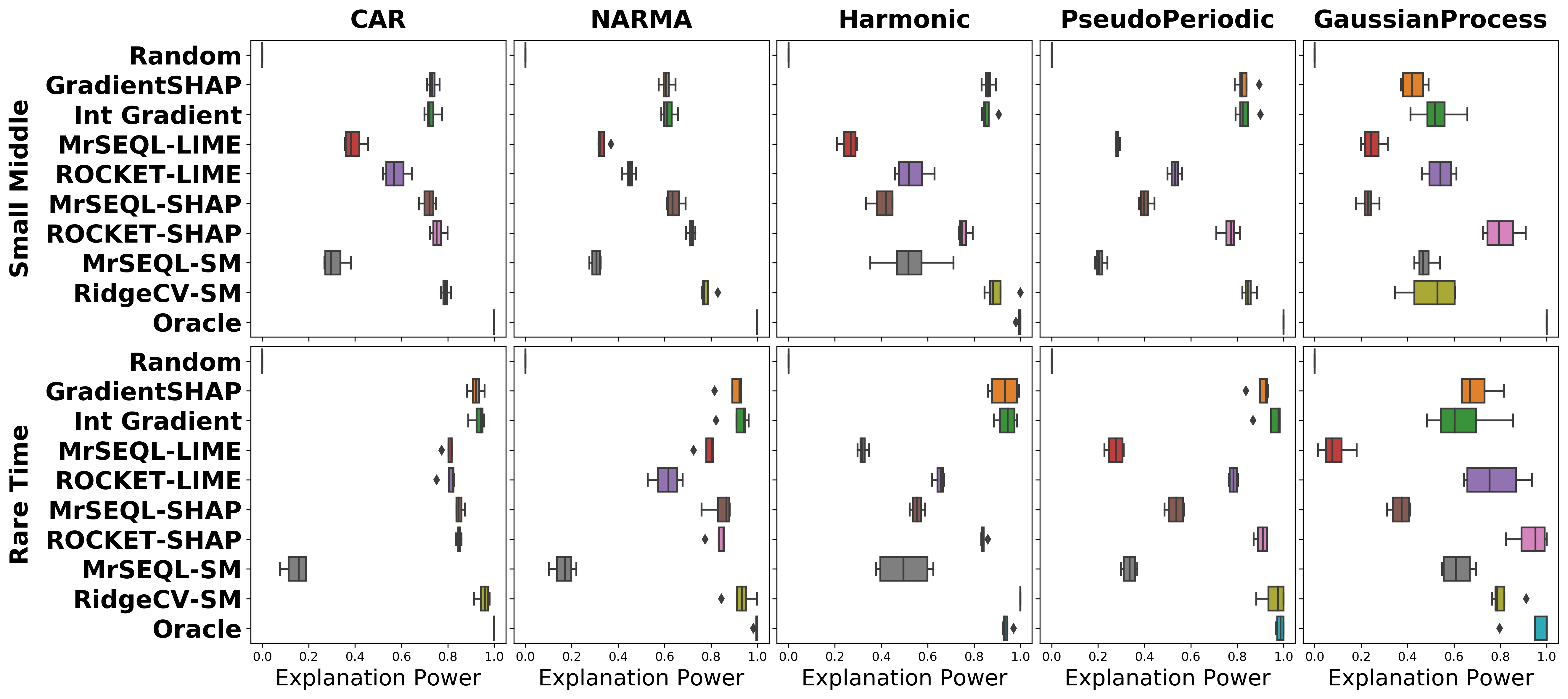
Figure 2: Impact of masking strategy on explanation power for each explanation method. A smaller box-range (which comes from 4 perturbation methods) indicates a smaller change of explanation power with different masking strategies. For datasets that are "easier" to classify by referees, this range is often smaller than that of "harder"-to-classify datasets. Having various perturbation strategies is useful due to common agreement in explanation power among different masking methods.

In this section, we describe our proposed methodology and related concepts. Specifically, we present the blueprint of AMEE in Figure 2. The framework involves a labelled time series dataset (split into training and test), a set of explanation methods to be compared, and a set of diverse Referee Classifiers. The output of the framework is the explanation power of each explanation method (see Table 1).

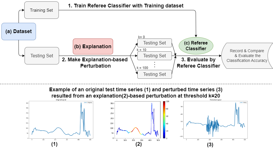
Figure 2: Upper figure: AMEE evaluation framework requires 3 elements: (a) a dataset that requires explanation evaluation, (b) a set of saliency-based explanations, and (c) a set of referee classifiers trained on a subset of (a). Bottom figure: a saliency-based time series explanation and an explanation-based perturbed time series.

3.1 Explanation and Saliency Map

3.1.1 Saliency-based explanation.

In the context of this paper, we only consider explanations in the form of saliency maps. A saliency map is numerically represented by a vector of weights $M=[w_{0},\dots,w_{d}]$ where $w_{i}\in\mathbb{R}$ and $d$ is the length of the time series. The value $w_{i}$ implies the importance (or saliency) of the time point $i$ in the process of prediction making. This vector can be obtained from annotation (by human) or computed by an explanation method. The explanation method can come from classification model itself (intrinsic explanation) or a black-box model coupled with a post-hoc method (post-hoc explanation).

3.1.2 Random Explanation.

An explanation generated through random sampling. The weights $w_{i}$ are drawn from a random uniform distribution. It serves as a baseline for any reasonable explanation method. While we expect this explanation to be the worst explanation in a ranking of several explanation methods, there exists situations where a random explanation outperforms a method-based explanation method. Specifically, when a method-based explanation highlights non-discriminative parts, or fails to identify any discriminative parts, that explanation can be considered worse than a random explanation.

3.1.3 Oracle Explanation.

In cases where we have explanation ground truth (e.g. for synthetic datasets), this should be the upper bound for any explanation method.

3.2 Explanation-based Perturbation

A good saliency-based explanation for a time series should highlight its discriminative part(s) that contain class-specific information to distinguish from other classes. Perturbation is the process of replacing the data points in the time series with artificial values. Perturbation of such discriminative part(s) will make it harder for a referee classifier to decide the class of this time series. As a result, the more informative the explanation, the higher the decrease in accuracy of a classifier, since that explanation-based perturbation knocks out important class-specific information in the respective time series.

Given a threshold $k$ ($0\leq k\leq 100$), the discriminative parts of a time series are defined as a set of $k*l/100$ time steps $D$ that have the highest weights in the saliency map $M$. In other words, the discriminative parts are identified by the top $k$-percentile in $M$. Varying $k$ allows us to control the scope of the perturbation. At $k=0$, the time series is kept as original; at $k=20$, only 20 percent of the time steps (that are most discriminative) are affected; at $k=100$ the entire time series is distorted.

3.3 Referee Classifiers

These classifiers form a committee of independent time series classifiers that are trained with the original training set. Our framework measures the impact of the perturbation on the predictions by the referees to evaluate the explanation methods.

3.4 Perturbation Strategy

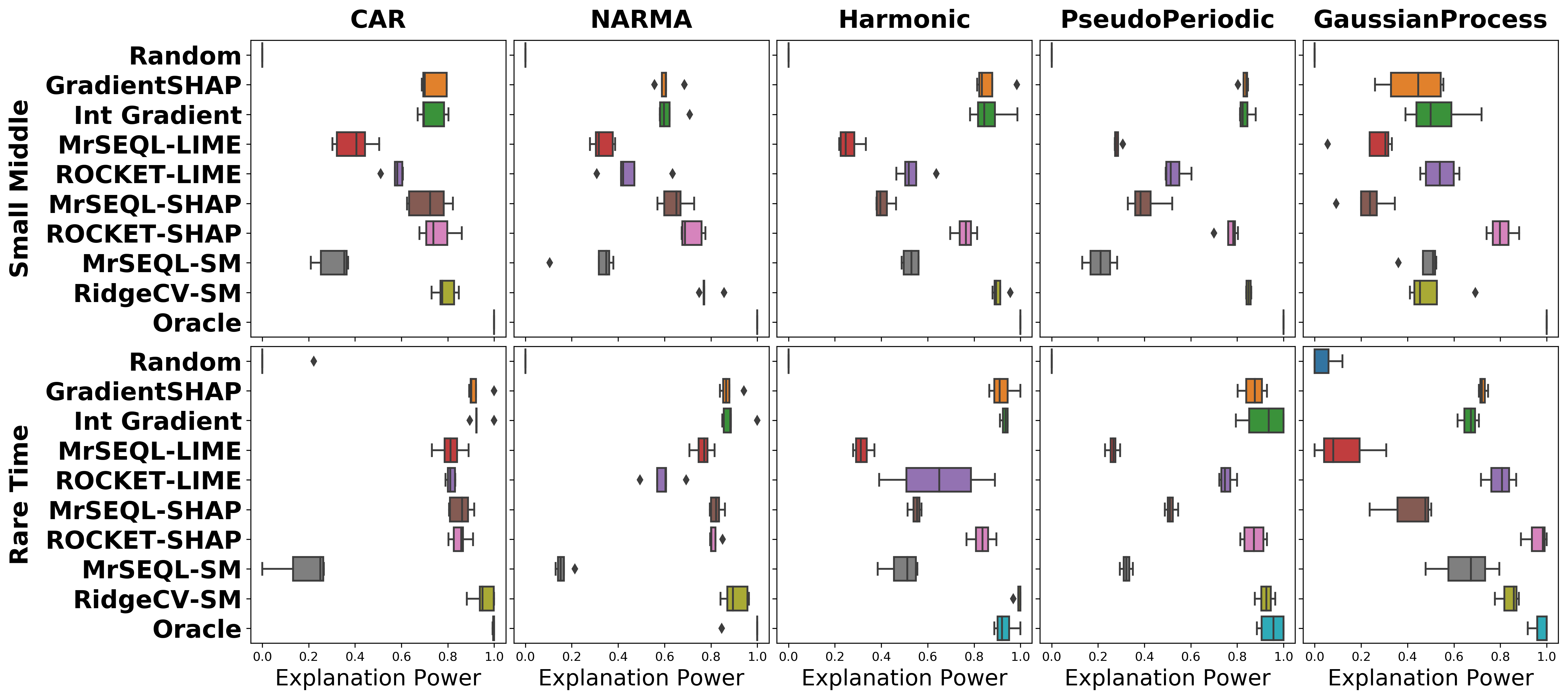
Figure 3: Impact of referees on explanation power for each explanation method. A smaller box-range (which comes from 5 referee classifiers) signals a smaller change of explanation power by different referees. Besides, in a specific dataset, the relative position of this range indicates the level of critical difference in opinions of referees in their votes. Nevertheless, having a committee of referees that are highly accurate is generally desirable.

In Figure 3 we explain and visualize the 4 strategies for masking the discriminative areas for a time series [28]. These strategies are either time-step dependent (local perturbation, using only i-th step information) or time-step independent (global perturbation), using either Gaussian-based or single value replacement.

Let $S$ be the number of time series in a dataset, each with $d$ time steps. We now want to perturb one out-of-sample time series of size $1\times d$, so its i-th value $x_{t}$ is replaced with new value $r_{t}$. We define the global and local profile for this time step perturbation as follows:

Local-based: $\hskip 14.22636pt\displaystyle\mu_{t}=\frac{1}{|S|}\sum_{s\in S}s_{t};\hskip 8.5359pt\sigma_{t}^{2}=\frac{1}{|S|-1}\sum_{s\in S}(s_{t}-\mu_{t})^{2}$

Global-based: $\hskip 8.5359pt\displaystyle\mu=\frac{1}{d|S|}\sum_{i=1}^{d}\sum_{s\in S}s_{i};\hskip 8.5359pt\sigma^{2}=\frac{1}{d|S|-1}\sum_{i=1}^{d}\sum_{s\in S}(s_{i}-\mu)^{2}$

With these local-based and global-based profiles, we can define the perturbation $r_{t}$ accordingly: Local mean: $r_{t}^{(1)}=\mu_{t}$; Local Gaussian: $r_{t}^{(2)}\sim\mathcal{N}(\mu_{t},\,\sigma_{t}^{2})$; Global mean: $r_{t}^{(3)}=\mu$; Global Gaussian: $r_{t}^{(4)}\sim\mathcal{N}(\mu,\,\sigma^{2})$. Figure 3 illustrates an example of how the 4 strategies effectively modify the original time series in its discriminative regions.

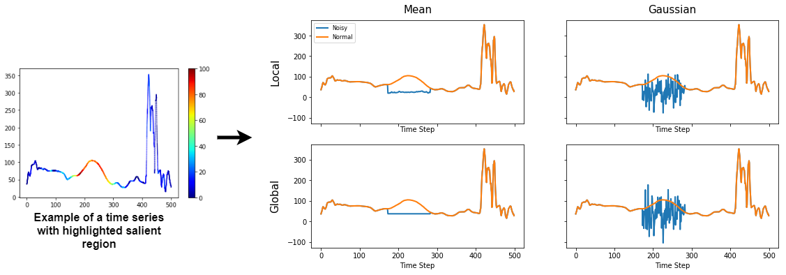
Figure 3: Masking strategy: An example time series with a known saliency map (left) is perturbed using mean or Gaussian noise using local time steps (local) or global time steps (global) across the entire dataset on its most salient region (top 20%).

3.5 AMEE: Model-Agnostic Framework for Explanation Evaluation in Time Series Classification

Figure 2 summarizes the components and steps in the AMEE framework. Our framework requires a labeled dataset ($D$) that needs explanation evaluation, a set of explanations ($M$) to evaluate, and a set of referee classifiers ($R$) to be trained on a subset of the dataset. With these elements, the following steps are done to record the necessary information to calculate evaluation metrics:

1. Split the labeled dataset $D$ into training ($D_{train}$) and test ($D_{test}$);

2. Train Referee Classifier(s) ($R$) with ($D_{train}$);

3. Use each explanation in $M$ to create a step-wise, explanation-based perturbation on $D_{test}$;

4. Measure the accuracy of trained referee $R$ on these perturbed datasets $D^{\prime}_{test}$.

The output of this process is the accuracy on the perturbed dataset $D^{\prime}_{test}$ at various thresholds ($k$), serving as an indicator of how strong an explanation-based perturbation impacts the referees. Significant drop in accuracy in the first few steps of explanation-based perturbation (e.g., at $k=10$) signals that meaningful, salient data points are disturbed. Hence, explanations that correctly identify such salient regions are likely to be informative.

3.5.1 Explanation AUC.

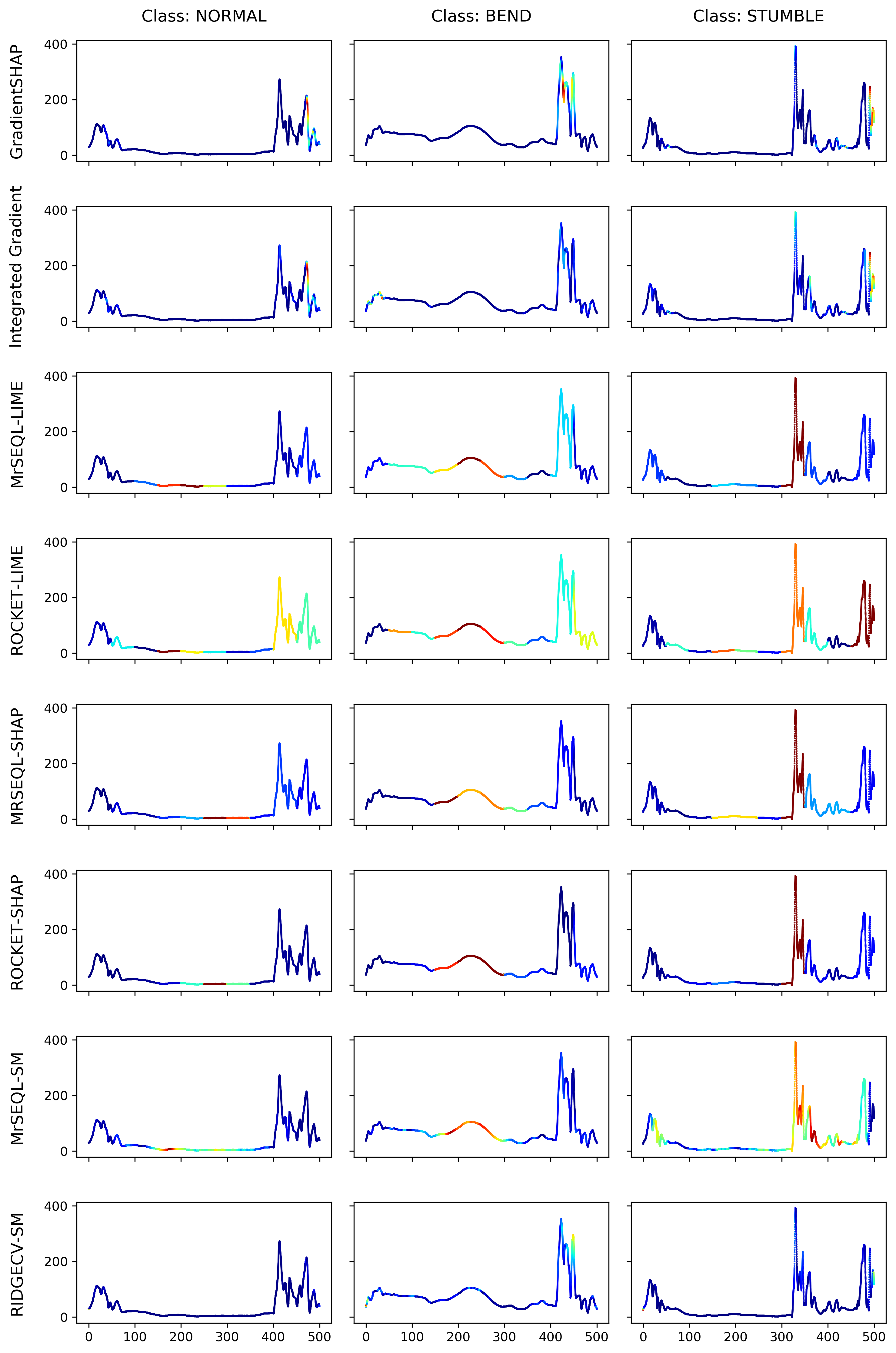
Figure 4: Visualization of all examined explanation methods on 3 classes of CMJ dataset. This figure is best read in combination with results in Table 5.

We measure the impact of perturbation guided by an explanation method by estimating the area under the curve (AUC) of its explanation-based perturbation. Specifically, the accuracy scores at each threshold ($k$) are translated into an Explanation-AUC ($EAUC$) using the trapezoidal rule. Smaller $EAUC$ means higher impact (accuracy loss) triggered by the explanation method (Figure 1 in Supplementary Materials). The Explanation AUC is computed for each combination of Perturbation - Referee - Explanation method (Figure 4: Step 1).

3.5.2 Metric Standardization & Explanation Power.

AMEE employs multiple perturbation strategies and multiple referee classifiers. As the EAUC measures depend on the choices of referees and the perturbation strategies, they are not directly comparable. The next steps (Figure 4: Step 2-5) standardize and aggregate the EAUC to compute the final output of the framework: the Explanation Power.

Step 2 rescales the Explanation AUC to the same range $[0,1]$ for each row (i.e. each pair of Referee and Perturbation). The red highlighted row is an example. After rescaling the Explanation AUC, the Average Scaled EAUC is computed in Step 3. It is basically the average of the column in Step 2. For example the Average Scaled EAUC of Rocket-SHAP is $(0.43+0.26+0.69+0.42+0.33+0.67)/6=0.47$.

In Step 4, the Average Scaled EAUC is again rescaled to the range between 0 and 1. The result is the Average Scaled Rank (lower is better). The Explanation Power is simply the inverse of Average Scaled Rank ($1-$ Average Scaled Rank), i.e., higher is better.

Details of this calculation are summarised in Algorithm 1

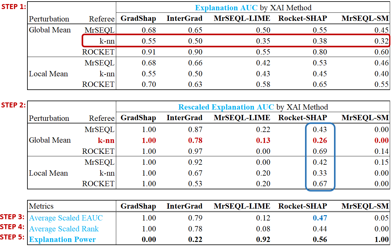
Figure 4: Metric Standardization and Explanation Power Calculation. This table illustrates an example of how Explanation Power is derived in a typical evaluation assessment, involved 2 perturbation strategies and 3 referees.

1

Input: Set of XAI methods ($M$), Types of Perturbation $T$, set of Referees ($R$), set of thresholds for important area ($k$), test accuracy ($acc_{M,T,R,k}$)

Output: Average Scaled Explanation AUC ($asEAUC_{M}$), Average Scaled Rank ($asRank_{M}$), Explanation Power ($ePower_{M}$)

2 Calculate Explanation AUC ($EAUC_{M,T,R}$) using $acc_{M,T,R,k}$

3 Calculate rescaled AUC ($sEAUC_{M,T,R}$) by Min/Max Rescaling $EAUC_{M,T,R}$

4 Calculate Average Scaled Explanation AUC ($asEAUC_{M}$) of each $M$ by averaging $sEAUC_{M,T,R}$ across $R$ and $T$

5 Calculate Average Scaled Rank ($asRank_{M}$) of each $M$ by Min/Max Rescaling $asEAUC_{M}$

Calculate Explanation Power ($ePower_{M}$) by 1 - $asEAUC_{M}$

Algorithm 1 AMEE: Calculate Explanation Power

4 Experiment

In this section, we evaluate the performance of the AMEE framework in 3 cases in ascending order of difficulty. In the simplest case, we want to confirm the validity of AMEE with synthetic datasets with known explanation ground-truth [19]. Next, we measure the performance of the framework with selected datasets from the UCR Time Series Archive [9]. Finally, we test our framework on a real dataset and compare the result with ground-truth explanations provided by a domain expert.

4.0.1 Referees.

We employ 5 candidates for referee classifiers in our experiment, selected based on their accuracy, speed and diversity of approaches [33]: baseline 1NN-DTW [7], MrSEQL [23], ROCKET [10], RESNET [16, 21] and WEASEL 2.0 [33]. As the choice of referees is a critical component in our framework, we carefully select classifiers that perform well in accuracy on all studied datasets. For a classifier to be selected in the referee committee, it has to achieve at least the average accuracy of all candidates for referee classifiers, and this number has to be higher than the theoretical accuracy achieved by a random classifier. In case the average accuracy is over 90%, the threshold to choose referees will be 90%. Details of the referee accuracy performance are presented in the Supplementary Materials.

4.0.2 Explanation Methods.

In our experiment, we evaluate 8 popular explanation methods, representing the various properties of explanation (Table 2).

Explanation	Type	Model	Explanation	Time-Series
Method		Specific	Scope	Specific
GradientSHAP	Post-hoc	Yes	Global	No
Integrated Gradient	Post-hoc	Yes	Global	No
MrSEQL-LIME	Post-hoc	No	Local	No
ROCKET-LIME	Post-hoc	No	Local	No
MrSEQL-SHAP	Post-hoc	No	Local	No
ROCKET-SHAP	Post-hoc	No	Local	No
MrSEQL-SM	Intrinsic	Yes	Global	Yes
RidgeCV-SM	Intrinsic	Yes	Global	No

Table 2: Summary of Explanation Methods properties

4.1 Evaluation for Synthetic Data with Known Ground Truth

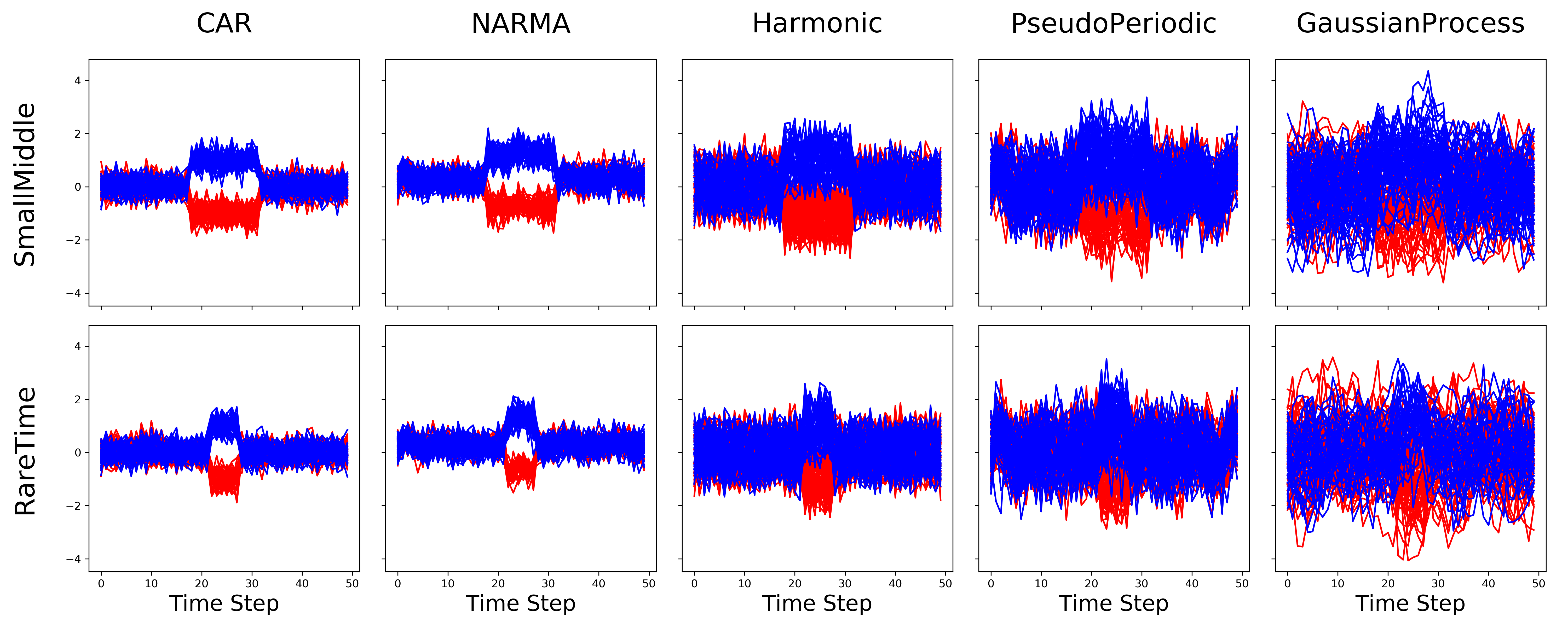
Figure 5: Visualization of the Synthetic Datasets. The columns describe the process used to create the dataset, while the row specifies the specific salient areas.

4.1.1 Data.

We work with 10 synthetic univariate datasets selected by taking the mid-channel from the benchmark generated by [19]. The datasets are created using five processes: (a) a standard continuous autoregressive time series with Gaussian noise (CAR), (b) sequences of standard non–linear autoregressive moving average (NARMA) time series with Gaussian noise, (c) nonuniformly sampled from a harmonic function (Harmonic), (d) nonuniformly sampled from a pseudo period function with Gaussian noise (Pseudo Periodic), and (e) Gaussian with zero mean and unit variance (Gaussian Process). The important areas, either a Small Middle part (30% of time series length) or a very small (Rare Time) part (10% of time series length), are created by adding or subtracting a constant $\mu$ ($\mu$ = 1) for the positive and negative class. The number of time steps is $T$ = 50. Each dataset comprises of 500 samples in training set and 100 samples in testing set. Figure 5 visualizes the two classes in the 10 datasets. Before presenting the experiment result of our evaluation on the synthetic datasets, we discuss the effect of the masking strategy and Referees, followed by a sanity check for source quality using model-agnostic post-hoc explanation methods.

4.1.2 Impact of Masking Strategy.

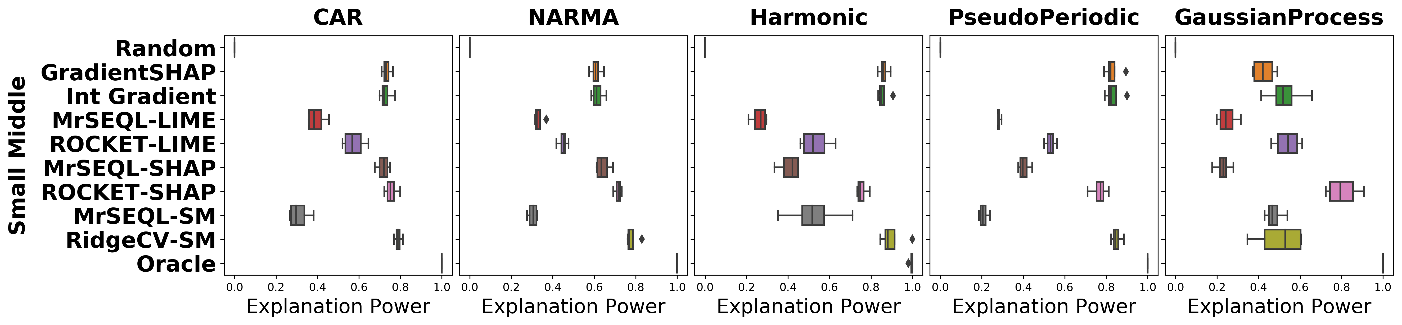
Figure 6: Impact of masking strategy on explanation power for each explanation method.

We investigate the effect of masking strategy in determining how one explanation compares to others. Specifically, we isolate the evaluation to one masking strategy and compare the effective explanation power with respect to four masking strategies. (Figure 6 ). In datasets which are "easier" to classify (i.e. most classifiers get close to 100% accuracy) such as CAR and NARMA, explanation power does not change with perturbation strategy. On the other hand, we observe a larger change in explanation power when data is harder to classify (for example, in SmallMiddle_GaussianProcess dataset). Nevertheless, extreme cases when explanation is Ground Truth (Oracle upper bound of explanation) and Random (lower bound of explanation) generally are the most and least informative informative methods, respectively. In the rest of the paper, we will leverage the advantage of having various types of perturbations and present the average explanation power by the four strategies presented in Section 3.

4.1.3 Impact of Referees.

Similar to the previous investigation on impact of masking strategy, we now inspect how explanation power changes with respect to referees and present the result in Figure 7 footnote 2. Here, we also notice a relatively consistent explanation power among different referee classifiers in datasets that are easier to classify (such as CAR- and NARMA-based datasets). In datasets that are harder-to-classify (for example, in Gaussian Process-based datasets), we observe a larger ranges in distribution of explanation methods over referee classifiers. Random and Oracle explanations both have their explanation power in expected values for the majority of the 10 datasets. Nevertheless, having a committee of referees that are highly accurate is desirable and is helpful in reducing bias that a single referee can introduce for a more stable evaluation.

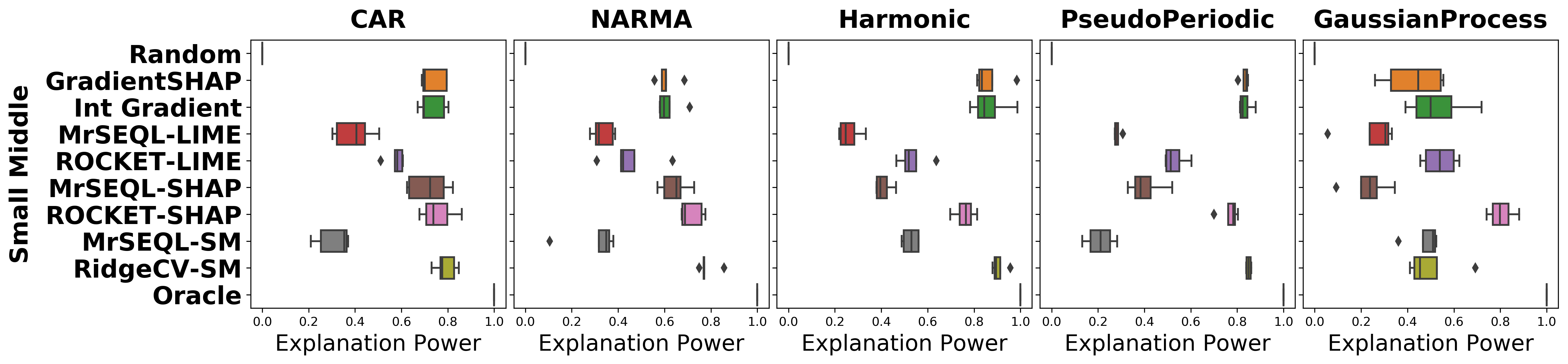
Figure 7: Impact of referees on explanation power for each explanation method.

4.1.4 Sanity check for Impact of Classifier Quality.

Model-agnostic post-hoc methods such as LIME and SHAP derive explanations based on a classifier of any types. Thus, these explanation are dependent on the performance of the base model. For example, the ROCKET-SHAP explanation is created by applying SHAP (explanation method) on ROCKET (source classifier). If a source classifier performs poorly (i.e., has low accuracy) on the sample dataset, the explanation based on that classifier could not be as good as one based on a more accurate source. In our experiment, we get LIME and SHAP explanations from two sources: MrSEQL classifier [23] and ROCKET [10]. We observe that ROCKET achieves higher accuracy than MrSEQL in datasets created from Pseudo Periodic, Harmonic, and Gaussian Process (Table 1 in Supplementary Materials). We compare the two pairs of explanation (MrSEQL-based and ROCKET-based) from LIME and SHAP and do a sanity check. Our experiment confirms that in both cases, ROCKET-LIME and ROCKET-SHAP are considered better explanation methods as compared to MrSEQL-LIME and MrSEQL-SHAP, respectively (Figure 6 and7). This sanity check confirms our intuition that the quality of the source classifier is an important factor in model-agnostic, post-hoc explanation methods such as LIME and SHAP.

4.1.5 Results.

Using a committee of 5 referees and 4 perturbation strategies, we evaluate 8 explanation methods together with the lower bound explanation (Random) and upper bound explanation (Oracle) using the AMEE framework. The resulting explanation power is presented in Table 3. We also compare the explanation methods with the ground truth explanation for each time points and calculate the F1-score (Table 4) to measure how good each method is in determining whether a timepoint is salient. Our result shows a high agreement between AMEE and the F1-score using ground truth time-point importance evaluation.

Dataset	Random	Grad SHAP	Int Gradient	MRSEQL -LIME	ROCKET -LIME	MRSEQL -SHAP	ROCKET -SHAP	MRSEQL -SM	RIDGECV -SM	Oracle
SM_CAR	0.00	0.73	0.73	0.39	0.58	0.72	0.76	0.31	0.79	1.00
SM_NARMA	0.00	0.61	0.62	0.33	0.45	0.64	0.71	0.30	0.78	1.00
SM_Harmonic	0.00	0.87	0.86	0.26	0.54	0.41	0.76	0.53	0.91	1.00
SM_PseudoPeriodic	0.00	0.83	0.84	0.28	0.53	0.40	0.77	0.21	0.85	1.00
SM_GaussianProcess	0.00	0.43	0.53	0.25	0.54	0.23	0.80	0.48	0.50	1.00
RT_CAR	0.00	0.92	0.93	0.81	0.81	0.85	0.85	0.14	0.95	1.00
RT_NARMA	0.00	0.90	0.92	0.79	0.61	0.85	0.84	0.17	0.93	1.00
RT_Harmonic	0.00	0.93	0.94	0.32	0.65	0.55	0.84	0.50	1.00	0.94
RT_PseudoPeriodic	0.00	0.92	0.96	0.28	0.79	0.54	0.92	0.34	0.97	1.00
RT_GaussianProcess	0.00	0.73	0.67	0.09	0.81	0.39	0.98	0.65	0.85	1.00

Table 3: Synthetic Datasets: Explanation Power by Methods.

Dataset	Random	Grad SHAP	Int Gradient	MRSEQL -LIME	ROCKET -LIME	MRSEQL -SHAP	ROCKET -SHAP	MRSEQL -SM	RIDGECV -SM	Oracle
SM_CAR	0.36	0.81	0.83	0.59	0.70	0.83	0.83	0.50	0.86	1.00
SM_NARMA	0.36	0.75	0.77	0.61	0.66	0.83	0.83	0.43	0.84	1.00
SM_Harmonic	0.36	0.56	0.59	0.51	0.52	0.63	0.80	0.44	0.61	1.00
SM_PseudoPeriodic	0.36	0.54	0.56	0.45	0.58	0.58	0.74	0.55	0.56	1.00
SM_GaussianProcess	0.36	0.19	0.24	0.42	0.50	0.38	0.65	0.61	0.16	1.00
RT_CAR	0.21	0.84	0.87	0.59	0.64	0.74	0.72	0.16	0.92	1.00
RT_NARMA	0.21	0.78	0.85	0.60	0.50	0.72	0.74	0.16	0.91	1.00
RT_Harmonic	0.21	0.42	0.47	0.29	0.39	0.46	0.69	0.29	0.65	1.00
RT_PseudoPeriodic	0.21	0.51	0.55	0.25	0.47	0.37	0.63	0.29	0.68	1.00
RT_GaussianProcess	0.21	0.21	0.20	0.22	0.37	0.25	0.51	0.34	0.33	1.00

Table 4: Synthetic Datasets: F1-score of important time points identified by Explanation Methods. Abbreviation: SM - Small Middle, RT - Rare Time.

4.2 Evaluation for UCR Time Series Archive

4.2.1 Data.

Selected univariate datasets from [9]. These datasets are of 6 types: Simulated (SIMUL), electrocardiogram (ECG), human motion (MOTION), device usage (DEVICE), object acvitities collected by sensors (SENSOR), spectroscopy (SPECTRO). We do not select image and audio datasets since explanations based on time domain univariate time series are not suitable for these types of data. Oracle explanation is not available for these datasets.

4.2.2 Results.

We test explanations for these datasets with AMEE and report the result in Table 5. Since we do not have ground truth for majority of these datasets, we use this experiment to show how AMEE can apply to real datasets. It is noticeable that Random explanation sometimes outperforms a method-base explanation. This is an expected situation, as some explanation methods may not work well with certain datasets, resulting in unreasonable explanations that misleadingly highlight non-discriminative parts as discriminative, or fail to identify any significant discriminative parts at all. In this situation, evaluation of random explanations can serve as a filter for reasonable explanation methods, and any methods that have lower performance should be seriously red-flagged.

Data Type	Dataset	Random	Grad SHAP	Int Gradient	MRSEQL -LIME	ROCKET -LIME	MRSEQL -SHAP	ROCKET -SHAP	MRSEQL -SM	RIDGECV -SM
ECG	ECG200	0.00	0.13	0.17	0.67	0.57	0.84	1.00	0.46	0.45
	ECG5000	0.00	1.00	0.99	0.67	0.57	0.61	0.82	0.30	0.29
	ECGFiveDays	0.54	0.77	0.71	0.39	0.54	0.91	1.00	0.00	0.27
	TwoLeadECG	0.39	0.17	0.18	0.44	0.40	0.92	1.00	0.05	0.00
MOTION	GunPoint	0.81	0.74	1.00	0.77	0.00	0.92	0.84	0.89	0.56
	CMJ	0.24	0.06	0.00	0.99	0.56	1.00	0.84	0.90	0.31
DEVICE	PowerCons	0.50	0.69	0.68	0.37	0.76	0.45	1.00	0.00	0.66
SPECTRO	Coffee	0.00	0.36	0.53	0.53	0.37	0.86	1.00	0.72	0.57
	Strawberry	0.65	0.41	0.43	0.91	0.66	1.00	0.40	0.70	0.00
SENSOR	Car	0.45	0.15	0.00	0.42	0.36	1.00	0.74	0.33	0.44
	ItalyPower	0.27	1.00	0.95	0.16	0.13	0.11	0.29	0.00	0.54
	Plane	0.75	0.80	0.78	0.50	0.00	0.67	1.00	0.19	0.32
	Sony1	0.23	0.84	0.80	0.21	0.52	0.32	1.00	0.00	0.83
	Sony2	0.32	0.99	1.00	0.45	0.41	0.37	0.82	0.00	0.57
	Trace	0.33	0.25	0.21	0.77	0.26	1.00	0.79	0.16	0.00
	Average	0.37	0.56	0.56	0.55	0.41	0.73	0.84	0.31	0.39
	Count of 1.00	0/15	2/15	2/15	0/15	0/15	4/15	7/15	0/15	0/15

Table 5: Explanation Power on UCR Datasets. Most informative method is highlighted in bold. The last row shows the count of occurrences when a method is selected as the most informative explanation according to AMEE.

4.3 Evaluation for Real Dataset with Expert Ground Truth

Oracle explanation is the upperbound for any explanation method, however, it is only available in synthetic datasets. Real datasets ground truth is often available in an approximate level of precision, e.g., specifying the relative position of the shape and areas of importance. This approximate ground truth is widely used in other papers in evaluating explanation methods for images [22, 40, 35] and it is fortunately available for CounterMovementJump (CMJ) among the datasets evaluated in Section 4.2 [23].

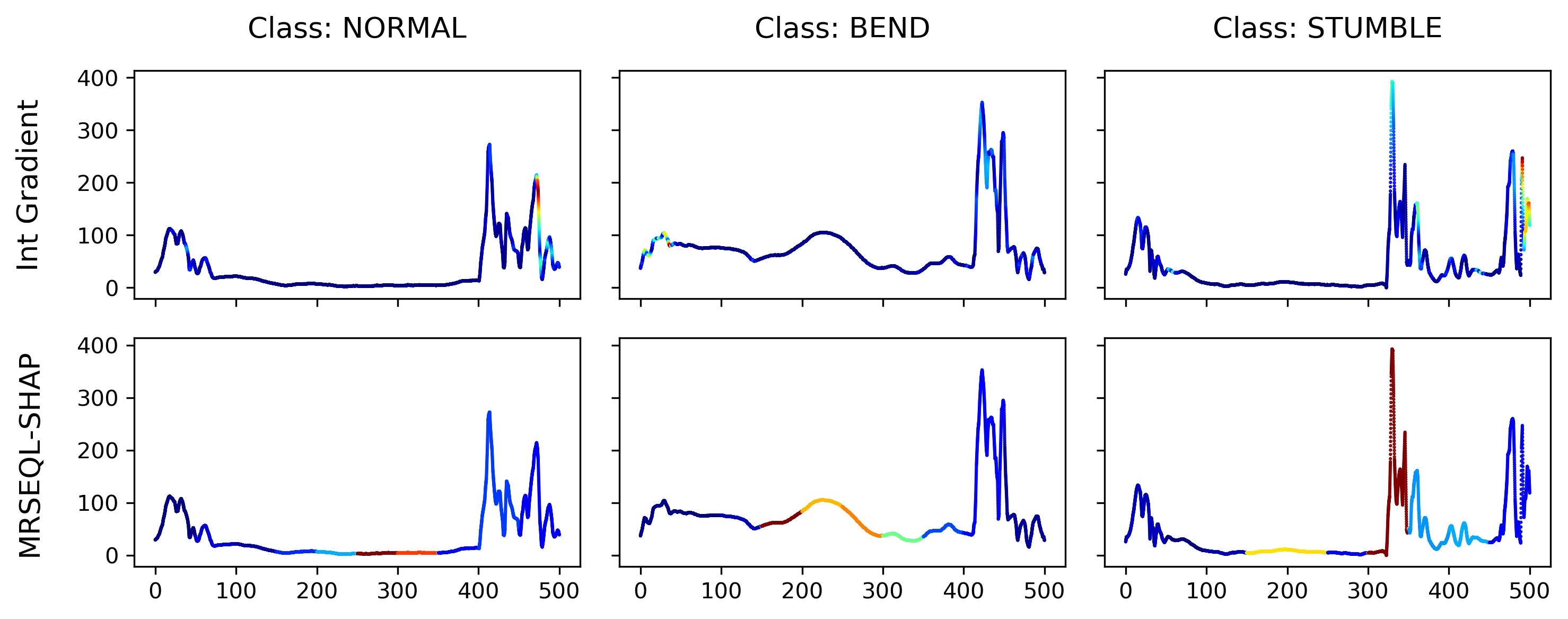
Figure 8: Visualization of worst explanation method (top row) and best explanation method (bottom row) identified by AMEE. Visualization of other explanations are presented in Supplementary Materials.

This dataset records the counter movement jumps of participants of 3 classes: Normal (jump done correctly), Bend (jump with knee bend), and Stumble (stumble at landing). According to the sports expert who recorded this data, the critical area for the first two classes (normal and bend) is the middle part, while that of the final class (stumble) is in the end of the time series records. In class Normal, this region is completely flat and indifferent from neighboring time point. The same region is characterized by a small hump in case participants’ knees in bending posture. In the Stumble class, the end of the time series is different from the previous two classes because of its very high, sharp peak due to very wrong landing position.

The result of AMEE for various explanation methods is also in Table 5. The CMJ row shows the top 3 explanations for this dataset are MrSEQL-SHAP (SHAP explanation based on MrSEQL classifier), MrSEQL-LIME (LIME explanation based on MrSEQL classifier), and MrSEQL-SM (saliency map obtained directly from MrSEQL classifier). We see a high agreement between these classifiers as they all correctly highlight the corresponding discriminative areas provided by the expert (Figure 8). In addition, methods that are pointed out by AMEE as unreliable are also shown to highlight incorrect explanations and do not agree with the opinion of the domain expert (e.g., Integrated Gradient).

4.4 Discussion

Our study carried over both synthetic and UCR datasets shows that AMEE can be conveniently used to computationally evaluate and compare different explanation methods. We recommend the use of AMEE with full knowledge about the essential elements of the method. First, referees should be selected carefully, using classifiers of acceptable accuracy as determined by the application requirements. Using a committee of multiple accurate referee classifiers is recommended to reduce possible biases that one referee could introduce and results in a more reliable evaluation. Second, having a variety of data perturbation methods is helpful, especially in case of hard-to-classify datasets. In addition, adding a random explanation while carrying out the evaluation with AMEE is helpful in identifying unreliable explanation methods. A worse-than-random explanation means that the explanation fails to trigger a change in referee classifiers when compared even to a random explanation, either not identifying the important areas, or not focusing on any important areas at all. Finally, we recommend adding SHAP-based methods to accurate base classifiers for testing and further evaluation, as our experiments show that SHAP-based explanations often outperform LIME-based explanations using the same base classifiers.

5 Conclusion

In this work we proposed AMEE, a Model-Agnostic Explanation Evaluation framework, for computationally assessing and ranking explanation methods for the time series classification task. We test the framework on both synthetic and UCR archive datasets to obtain explanation evaluations for a wide variety of common explanation methods for time series, covering different aspects of explanation including type, scope and model dependency. Our experiments show a high agreement of the Explanation Power (measured by AMEE) in the synthetic datasets with the Oracle explanation (ground truth at time-point precision) and the Expert explanation in a real dataset (ground truth provided by a domain expert). This evaluation approach can be used to select appropriate explanation methods for application users or shortlist candidate methods for more detailed and expensive user studies. Besides, AMEE could potentially pinpoint the inherent problems, such as biases, that may exist in the training data. This evaluation further empowers machine learning to discover new knowledge from the data. Future work includes devising a robust, AMEE-optimized, explanation method and using data experts to evaluate the validity and potential of knowledge discovery using this framework in biomedical and heathcare-related tasks such as genetic data understanding and sports analytics.

Supplementary Materials

Dataset	MrSEQL	k-nn	RESNET	ROCKET	WEASEL
SM_CAR	1.00	1.00	1.00	1.00	1.00
SM_NARMA	1.00	1.00	1.00	1.00	1.00
SM_Harmonic	0.85	1.00	1.00	1.00	1.00
SM_PseudoPeriodic	0.84	1.00	1.00	1.00	1.00
SM_GaussianProcess	0.64	0.94	0.84	0.89	0.85
RT_CAR	1.00	1.00	1.00	1.00	1.00
RT_NARMA	1.00	1.00	1.00	1.00	1.00
RT_Harmonic	0.80	1.00	0.96	1.00	0.97
RT_PseudoPeriodic	0.79	0.99	0.94	0.99	0.92
RT_GaussianProcess	0.51	0.87	0.64	0.80	0.73

Table 1: Classifier accuracy on synthetic datasets. Classifiers that are selected as referees are in bold

Dataset	MrSEQL	k-nn	RESNET	ROCKET	WEASEL
CBF	1.00	0.85	0.97	1.00	0.98
TwoPatterns	1.00	0.91	0.99	1.00	1.00
ECG200	0.89	0.88	0.83	0.90	0.89
ECG5000	0.94	0.92	0.92	0.95	0.95
ECGFiveDays	1.00	0.80	0.92	1.00	0.97
TwoLeadECG	0.99	0.75	0.94	1.00	1.00
GunPoint	0.99	0.91	0.97	1.00	1.00
CMJ	0.96	0.92	0.92	0.97	0.97
PowerCons	0.88	0.98	0.91	0.96	0.93
Coffee	1.00	1.00	0.96	1.00	1.00
Strawberry	0.96	0.95	0.94	0.98	0.98
Car	0.85	0.73	0.40	0.90	0.92
ItalyPower	0.91	0.96	0.95	0.97	0.96
Plane	1.00	0.96	0.87	1.00	1.00
Sony1	0.75	0.70	0.89	0.92	0.94
Sony2	0.88	0.86	0.88	0.92	0.95
Trace	1.00	0.76	0.75	1.00	1.00

Table 2: Classifier accuracy on UCR datasets. Classifiers that are selected as referees are in bold. Abbreviations: CounterMovementJump - CMJ, ItalyPower - ItalyPowerDemand, Sony1/2 -SonyAIBORobotSurface1/2

References

- [1] Adebayo, J., Gilmer, J., Muelly, M., Goodfellow, I., Hardt, M., Kim, B.: Sanity checks for saliency maps. Advances in neural information processing systems 31 (2018)
- [2] Agarwal, S., Nguyen, T.T., Nguyen, T.L., Ifrim, G.: Ranking by aggregating referees: Evaluating the informativeness of explanation methods for time series classification. In: International Workshop on Advanced Analytics and Learning on Temporal Data. pp. 3–20 (2021)
- [3] Avci, A., Bosch, S., Marin-Perianu, M., Marin-Perianu, R., Havinga, P.: Activity recognition using inertial sensing for healthcare, wellbeing and sports applications: A survey. In: 23th International conference on architecture of computing systems 2010. pp. 1–10 (2010)
- [4] Bostrom, N., Yudkowsky, E.: The ethics of artificial intelligence. In: Artificial intelligence safety and security, pp. 57–69. Chapman and Hall/CRC (2018)
- [5] Brown, T., Mann, B., Ryder, N., Subbiah, M., Kaplan, J.D., Dhariwal, P., Neelakantan, A., Shyam, P., Sastry, G., Askell, A., others: Language models are few-shot learners. Advances in neural information processing systems 33, 1877–1901 (2020)
- [6] Caruana, R., Lou, Y., Gehrke, J., Koch, P., Sturm, M., Elhadad, N.: Intelligible Models for HealthCare: Predicting Pneumonia Risk and Hospital 30-Day Readmission. In: Proceedings of the 21th ACM SIGKDD International Conference on Knowledge Discovery and Data Mining. pp. 1721–1730. KDD ’15, Association for Computing Machinery, New York, NY, USA (2015). https://doi.org/10.1145/2783258.2788613, https://doi.org/10.1145/2783258.2788613
- [7] Cover, T., Hart, P.: Nearest neighbor pattern classification. IEEE Transactions on Information Theory 13(1), 21–27 (1967). https://doi.org/10.1109/TIT.1967.1053964
- [8] Crabbé, J., Van Der Schaar, M.: Explaining Time Series Predictions with Dynamic Masks. In: Meila, M., Zhang, T. (eds.) Proceedings of the 38th International Conference on Machine Learning. Proceedings of Machine Learning Research, vol. 139, pp. 2166–2177. PMLR (1 2021), https://proceedings.mlr.press/v139/crabbe21a.html
- [9] Dau, H.A., Bagnall, A.J., Kamgar, K., Yeh, C.C.M., Zhu, Y., Gharghabi, S., Ratanamahatana, C.A., Keogh, E.J.: The UCR Time Series Archive. CoRR abs/1810.07758 (2018), http://arxiv.org/abs/1810.07758
- [10] Dempster, A., Petitjean, F., Webb, G.I.: ROCKET: exceptionally fast and accurate time series classification using random convolutional kernels. Data Mining and Knowledge Discovery 34(5), 1454–1495 (2020)
- [11] Devlin, J., Chang, M.W., Lee, K., Toutanova, K.: Bert: Pre-training of deep bidirectional transformers for language understanding. arXiv preprint arXiv:1810.04805 (2018)
- [12] Doshi-Velez, F., Kim, B.: Towards a rigorous science of interpretable machine learning. arXiv preprint arXiv:1702.08608 (2017)
- [13] Frizzarin, M., Visentin, G., Ferragina, A., Hayes, E., Bevilacqua, A., Dhariyal, B., Domijan, K., Khan, H., Ifrim, G., Nguyen, T.L., Meagher, J., Menchetti, L., Singh, A., Whoriskey, S., Williamson, R., Zappaterra, M., Casa, A.: Classification of cow diet based on milk Mid Infrared Spectra: A data analysis competition at the “International Workshop on Spectroscopy and Chemometrics 2022”. Chemometrics and Intelligent Laboratory Systems 234, 104755 (3 2023). https://doi.org/10.1016/j.chemolab.2023.104755, https://linkinghub.elsevier.com/retrieve/pii/S0169743923000059
- [14] Goodfellow, I., Shlens, J., Szegedy, C.: Explaining and Harnessing Adversarial Examples. In: International Conference on Learning Representations (2015), http://arxiv.org/abs/1412.6572
- [15] Guidotti, R.: Evaluating local explanation methods on ground truth. Artificial Intelligence 291, 103428 (2021)
- [16] He, K., Zhang, X., Ren, S., Sun, J.: Deep residual learning for image recognition. In: Proceedings of the IEEE conference on computer vision and pattern recognition. pp. 770–778 (2016)
- [17] Hosmer Jr, D.W., Lemeshow, S., Sturdivant, R.X.: Applied logistic regression, vol. 398. John Wiley & Sons (2013)
- [18] Ifrim, G., Wiuf, C.: Bounded coordinate-descent for biological sequence classification in high dimensional predictor space. In: Proceedings of the 17th ACM SIGKDD international conference on knowledge discovery and data mining. pp. 708–716 (2011)
- [19] Ismail, A.A., Gunady, M., Corrada Bravo, H., Feizi, S.: Benchmarking Deep Learning Interpretability in Time Series Predictions. In: Larochelle, H., Ranzato, M., Hadsell, R., Balcan, M.F., Lin, H. (eds.) Advances in Neural Information Processing Systems. vol. 33, pp. 6441–6452. Curran Associates, Inc. (2020), https://proceedings.neurips.cc/paper/2020/file/47a3893cc405396a5c30d91320572d6d-Paper.pdf
- [20] Ismail Fawaz, H., Forestier, G., Weber, J., Idoumghar, L., Muller, P.A.: Accurate and interpretable evaluation of surgical skills from kinematic data using fully convolutional neural networks. International journal of computer assisted radiology and surgery 14(9), 1611–1617 (2019)
- [21] Ismail Fawaz, H., Forestier, G., Weber, J., Idoumghar, L., Muller, P.A.: Deep learning for time series classification: a review. Data Mining and Knowledge Discovery 33(4) (2019). https://doi.org/10.1007/s10618-019-00619-1
- [22] Kim, B., Wattenberg, M., Gilmer, J., Cai, C., Wexler, J., Viegas, F., others: Interpretability beyond feature attribution: Quantitative testing with concept activation vectors (tcav). In: International conference on machine learning. pp. 2668–2677 (2018)
- [23] Le Nguyen, T., Gsponer, S., Ilie, I., O’Reilly, M., Ifrim, G.: Interpretable time series classification using linear models and multi-resolution multi-domain symbolic representations. Data Mining and Knowledge Discovery 33(4), 1183–1222 (7 2019). https://doi.org/10.1007/s10618-019-00633-3
- [24] Lin, J., Keogh, E., Wei, L., Lonardi, S.: Experiencing SAX: a novel symbolic representation of time series. Data Mining and knowledge discovery 15(2), 107–144 (2007)
- [25] Lipton, Z.C.: The Mythos of Model Interpretability: In Machine Learning, the Concept of Interpretability is Both Important and Slippery. Queue 16(3), 31–57 (6 2018). https://doi.org/10.1145/3236386.3241340, https://doi.org/10.1145/3236386.3241340
- [26] Lundberg, S.M., Lee, S.I.: A Unified Approach to Interpreting Model Predictions. In: Guyon, I., Luxburg, U.V., Bengio, S., Wallach, H., Fergus, R., Vishwanathan, S., Garnett, R. (eds.) Advances in Neural Information Processing Systems 30, pp. 4765–4774. Curran Associates, Inc. (2017), http://papers.nips.cc/paper/7062-a-unified-approach-to-interpreting-model-predictions.pdf
- [27] Lundberg, S.M., Nair, B., Vavilala, M.S., Horibe, M., Eisses, M.J., Adams, T., Liston, D.E., Low, D.K.W., Newman, S.F., Kim, J., others: Explainable machine-learning predictions for the prevention of hypoxaemia during surgery. Nature biomedical engineering 2(10), 749–760 (2018)
- [28] Mujkanovic, F., Doskoc, V., Schirneck, M., Schäfer, P., Friedrich, T.: timeXplain - A Framework for Explaining the Predictions of Time Series Classifiers. CoRR abs/2007.07606 (2020), https://arxiv.org/abs/2007.07606
- [29] Nguyen, T.T., Le Nguyen, T., Ifrim, G.: A model-agnostic approach to quantifying the informativeness of explanation methods for time series classification. In: International Workshop on Advanced Analytics and Learning on Temporal Data. pp. 77–94 (2020)
- [30] Petitjean, F., Forestier, G., Webb, G.I., Nicholson, A.E., Chen, Y., Keogh, E.: Dynamic time warping averaging of time series allows faster and more accurate classification. In: 2014 IEEE international conference on data mining. pp. 470–479 (2014)
- [31] Ramgopal, S., Thome-Souza, S., Jackson, M., Kadish, N.E., Fernández, I.S., Klehm, J., Bosl, W., Reinsberger, C., Schachter, S., Loddenkemper, T.: Seizure detection, seizure prediction, and closed-loop warning systems in epilepsy. Epilepsy & behavior 37, 291–307 (2014)
- [32] Ribeiro, M.T., Singh, S., Guestrin, C.: "Why should i trust you?" Explaining the predictions of any classifier. In: Proceedings of the ACM SIGKDD International Conference on Knowledge Discovery and Data Mining (2016). https://doi.org/10.1145/2939672.2939778
- [33] Schäfer, P., Leser, U.: WEASEL 2.0–A Random Dilated Dictionary Transform for Fast, Accurate and Memory Constrained Time Series Classification. arXiv preprint arXiv:2301.10194 (2023)
- [34] Schlegel, U., Arnout, H., El-Assady, M., Oelke, D., Keim, D.A.: Towards A Rigorous Evaluation Of XAI Methods On Time Series. In: 2019 IEEE/CVF International Conference on Computer Vision Workshop (ICCVW). pp. 4197–4201 (2019). https://doi.org/10.1109/ICCVW.2019.00516
- [35] Selvaraju, R.R., Cogswell, M., Das, A., Vedantam, R., Parikh, D., Batra, D.: Grad-cam: Visual explanations from deep networks via gradient-based localization. In: Proceedings of the IEEE international conference on computer vision. pp. 618–626 (2017)
- [36] Smilkov, D., Thorat, N., Kim, B., Viégas, F., Wattenberg, M.: Smoothgrad: removing noise by adding noise. arXiv preprint arXiv:1706.03825 (2017)
- [37] Štrumbelj, E., Kononenko, I.: Explaining prediction models and individual predictions with feature contributions. Knowledge and information systems 41, 647–665 (2014)
- [38] Sundararajan, M., Taly, A., Yan, Q.: Axiomatic attribution for deep networks. In: International conference on machine learning. pp. 3319–3328 (2017)
- [39] Suresh, H., Hunt, N., Johnson, A., Celi, L.A., Szolovits, P., Ghassemi, M.: Clinical intervention prediction and understanding with deep neural networks. In: Machine Learning for Healthcare Conference. pp. 322–337 (2017)
- [40] Zhou, B., Khosla, A., Lapedriza, A., Oliva, A., Torralba, A.: Learning Deep Features for Discriminative Localization. In: Proceedings of the IEEE Computer Society Conference on Computer Vision and Pattern Recognition. vol. 2016-December, pp. 2921–2929. IEEE Computer Society (12 2016). https://doi.org/10.1109/CVPR.2016.319