Investigating the Impact of Metallicity on Star Formation in the Outer Galaxy.
I. VLT/KMOS Survey of Young Stellar Objects in Canis Major

Abstract

The effects of metallicity on the evolution of protoplanetary disks may be studied in the outer Galaxy where the metallicity is lower than in the solar neighborhood. We present the VLT/KMOS integral field spectroscopy in the near-infrared of $\sim$120 candidate young stellar objects (YSOs) in the CMa-$\ell$224 star-forming region located at a Galactocentric distance of 9.1 kpc. We characterise the YSO accretion luminosities and accretion rates using the hydrogen Br$\gamma$ emission and find the median accretion luminosity of $\log{(L_{\rm acc})}=-0.82^{+0.80}_{-0.82}L_{\odot}$. Based on the measured accretion luminosities, we investigate the hypothesis of star formation history in the CMa-$\ell$224. Their median values suggest that Cluster C, where most of YSO candidates have been identified, might be the most evolved part of the region. The accretion luminosities are similar to those observed toward low-mass YSOs in the Perseus and Orion molecular clouds, and do not reveal the impact of lower metallicity. Similar studies in other outer Galaxy clouds covering a wide range of metallicities are critical to gain a complete picture of star formation in the Galaxy.

1 Introduction

Stars form as a result of complex physico-chemical processes initiated by the gravitational collapse of a dense and cold molecular cloud. The formation of a rotating envelope and the embedded disk is associated with the ejection of jets and disk winds, together responsible for the removal of the angular momentum (e.g., Frank et al., 2014). The interaction between jets/winds and the envelope leads to the formation of outflow cavities and the dispersion of some mass reservoir (van Kempen et al., 2010; Visser et al., 2012). Shock waves at the outflow/envelope interface compress and heat the envelope material to hundreds or thousands of K, even around low-mass protostars (Kristensen et al., 2017; Karska et al., 2018).

The net mass growth of a young star is a balance between the mass accretion from the envelope-disk system and the mass ejection by jets and winds. The main accretion phase occurs during the earliest evolutionary stages of a young stellar object (YSO; Class 0 and Class I), accompanied by collimated H₂ jets (Davis & Eisloeffel, 1995; Stanke et al., 2002; Kristensen et al., 2007) and more extended molecular outflows (van der Marel et al., 2013; Tobin et al., 2016; Mottram et al., 2017). Once the protostar evolves into Class II, the envelope mass reservoir is mostly depleted, the accretion rate decreases, and the outflow opening angle widens (Offner et al., 2011; Agra-Amboage et al., 2014). The gradual decrease of accretion rates (Manara et al., 2012; Ansdell et al., 2017; Testi et al., 2022) is accompanied by decreasing mass loss rates and a transition from mostly molecular to atomic/ionic outflows (Nisini et al., 2015; Bally, 2016).

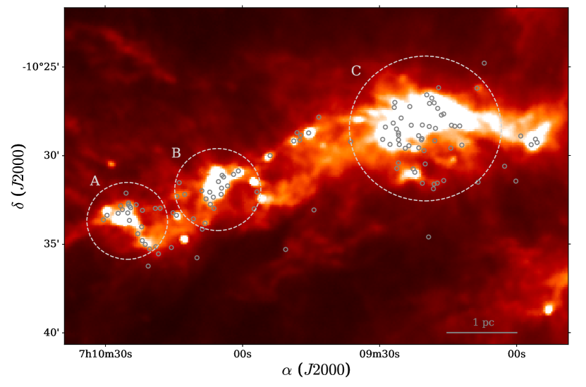
Figure 1: Herschel/SPIRE 250 $\mu$m image of the main filament in the CMa-$\ell$224 star-forming region. Grey circles show the positions of YSO candidates observed with VLT/KMOS, while light-grey dashed ellipses indicate regions hosting clusters of sources with the extended 4.5 $\mu$m emission (most likely tracing outflows) defined in (Sewiło et al., 2019, Clusters A, B, and C). North is up, east to the left.

The location of a star-forming region in the Galaxy may influence the process of mass assembly. In the outer Galaxy, the gas surface density in molecular clouds is known to be lower than those in the solar neighborhood (Roman-Duval et al., 2010). The decrease of metallicity with Galactocentric radius, traced by Fe or O abundance gradients, also translates to lower dust and molecular gas abundances (Sodroski et al., 1997; Lépine et al., 2011; Hawkins, 2022). Additionally, lower cosmic-ray fluxes and the interstellar UV radiation field reduce the amount of gas and dust heating (Bloemen et al., 1984). These factors may affect physical and chemical conditions in star forming regions and result in globally lower star formation rates and efficiencies in the outer Galaxy (Kennicutt & Evans, 2012; Heyer & Dame, 2015; Djordjevic et al., 2019).

Recent infrared studies revealed significant star formation activity in the Canis Major star-forming region in the outer Galaxy (Fischer et al., 2016; Sewiło et al., 2019). The 2.${}^{\circ}5\times 1.^{\circ}4$ region in Canis Major dubbed CMa-$\ell 224$ centered on ($l$, $b$)=(224.^∘5, $-$0.^∘65) is particularly interesting because it hosts clusters of sources with extended 4.5 $\mu$m emission (likely tracing outflows), many of which were identified as YSOs (Sewiło et al., 2019). CMa-$\ell 224$ is located at a distance of 0.92 kpc from the Sun and 9.1 kpc from the Galactic Center (e.g., Claria 1974), where a subsolar metallicity is predicted by the O/H Galactocentric radial gradients determined based on the observations of H ii regions ($Z$$\sim$$0.55-0.73$ $Z_{\odot}$: Balser et al. 2011; Fernández-Martín et al. 2017; Esteban & García-Rojas 2018). CMa-$\ell 224$ corresponds to a local peak of the H₂ column density and the lowest dust temperatures in the far-infrared observations of the outer Galaxy by the “Herschel infrared Galactic Plane Survey” (Hi-GAL; Molinari et al. 2010). The region contains a complex network of star-forming filaments (Figure 1, Elia et al., 2013; Schisano et al., 2014) and a widespread emission in CO and its isotopologues, tracing dense, molecular gas (Olmi et al., 2016; Benedettini et al., 2020; Lin et al., 2021).

Sewiło et al. (2019) identified 294 YSO candidates in CMa-$\ell$224 based on the photometric data from the near- and mid-infrared catalogs: Spitzer’s “GLIMPSE360: Completing the Spitzer Galactic Plane Survey” (PI: B. Whitney), the Two Micron All Sky Survey (2MASS; Skrutskie et al. 2006), and the AllWISE catalog that combines the “Wide-field Infrared Survey Explorer” (WISE; Wright et al. 2010) and NEOWISE (Mainzer et al., 2011) data. Some YSO candidates in CMa-$\ell$224 are associated with the extended 4.5 $\mu$m emission (Extended Green Objects, EGOs; Cyganowski et al. 2008), likely dominated by the H₂ line emission from outflow shocks (e.g., Cyganowski et al. 2011). The Spectral Energy Distribution (SED) fitting with the Robitaille (2017a) YSO models identified 37 sources with envelopes, i.e., Class 0/I YSOs. Thus, CMa-$\ell$224 offers an opportunity to evaluate how metallicity affects the ongoing star formation in a region that is significantly closer than, for example, the Magellanic Clouds.

In this paper, we address the following questions. What are the mass accretion rates in YSOs in CMa-$\ell$224? How are they connected to the star formation scenarios in this region? Is there any impact of the reduced gas metallicity on the accretion properties of YSOs in CMa-$\ell$224?

To this end, we present the results of the integral field spectroscopy of 124 YSO candidates in the CMa-$\ell$224 star-forming region using the $K$-band Multi Object Spectrograph (KMOS; Sharples et al. 2013) on the Very Large Telescope (VLT). VLT/KMOS provides $2\hbox to0.0pt{.\hss}{{}^{\prime\prime}}8\times 2\hbox to0.0pt{.\hss}{{}^{\prime\prime}}8$ spectral maps in ro-vibrational H₂ lines, hydrogen Br$\gamma$, and CO bandhead at 2.3 $\mu$m. At the distance of CMa-$\ell$224, we obtained $\sim$$2580\times 2580$ au maps at the physical resolution of 184 au.

The paper is organized as follows. In Section 2, we describe our sample selection, KMOS observations, and data reduction. In Section 3, we present the continuum and line emission maps, provide the statistics on line detections, discuss gas spatial distribution and describe calculations of the mass accretion rates. In Section 4, we discuss the results in the context of the star formation scenarios in CMa-$\ell$224, and in Section 5, we present the summary and conclusions.

This paper is the first in a series presenting the multi-wavelength spectroscopy of YSO candidates in the CMa-$\ell$224 star-forming region. Two forthcoming papers will discuss the ¹³CO and C¹⁸O 2-1 observations of YSO candidates in the main filament in CMa-$\ell$224 with the Atacama Large Millimeter/submillimeter Array (ALMA; Koprowski et al., in prep.), and the spectral types and excess continuum measurements toward YSO candidates in the second brightest filament in the region using the SpeX instrument at the NASA Infrared Telescope Facility (IRTF; Le et al., in prep.).

2 KMOS Observations and Data Reduction

We used VLT/KMOS to observe YSO candidates in the CMa-$\ell$224 star-forming region as part of the ESO programme 0102.C-0914(A) (PI: A. Karska). The sources were selected from the catalogue of YSO candidates from Sewiło et al. (2019) based on their 2MASS $K$-band brightness and location within two KMOS patrol fields.

Targets were selected from the $K$-band magnitude range of 9.5–15 to ensure a sufficient signal-to-noise ratio (SNR) without saturation for a single integration time applied to all exposures.

KMOS is a second-generation instrument operating in the near-infrared (near-IR) at the B Nasmyth focus of the VLT Unit Telescope 1 on Paranal in Chile, in operation since November 2012 (Sharples et al., 2013). It performs Integral Field Spectroscopy (IFS) for up to 24 targets simultaneously. Each of the 24 pick-off arms is connected to one of three identical spectrographs and detectors. KMOS arms are allocated in two planes (“top” and “bottom”) to avoid interference between them. The patrol field is 7$\hbox to0.0pt{.\hss}{{}^{\prime}}$2 in diameter, the size of each IFU is $2\hbox to0.0pt{.\hss}{{}^{\prime\prime}}8\times 2\hbox to0.0pt{.\hss}{{}^{\prime\prime}}8$, and the spatial sampling (spaxel size) is $0\hbox to0.0pt{.\hss}{{}^{\prime\prime}}2\times 0\hbox to0.0pt{.\hss}{{}^{\prime\prime}}2$.

Observations were prepared using the KMOS Arm Allocator (KARMA) and p2, a web-based tool for preparation of the Phase 2 material. The observations were performed in October and December 2018.

We used the K grating with the spectral range from 1.93 to 2.50 $\mu$m and resolving power $R$ of $\sim$4000, with a spectral sampling $\Delta\lambda$ of $\sim$2.8 Å per spectral element, corresponding to $\sim$39.7 km s^-1 at 2.1218 $\mu$m. The total integration time for each pointing was 1300 s with 5 single exposures of 260 s, dithered by 0$\hbox to0.0pt{.\hss}{{}^{\prime\prime}}$2.

The Nod-to-Sky mode was used to observe sources in both the ‘science’ and ‘sky’ pointings. The arms originally observing targets were next directed to the sky area, while those observing the sky were capturing science objects in the ‘sky’ pointing, usually offset by a few arcmin. One of the pick-off arms was broken during semester 102, which resulted in a lack of observations of 6 sources.

Table 1 shows the summary of the atmospheric conditions during our KMOS observations. The amount of precipitatable water vapour (PWV) was in the range from $\sim$2.5 to 4 mm, and the sky was covered with thin cirrus (TN). Seeing measured at the observatory site was typically below 1^′′ with the point spread function (PSF) of the data in the 0$\hbox to0.0pt{.\hss}{{}^{\prime\prime}}$4–0$\hbox to0.0pt{.\hss}{{}^{\prime\prime}}$7 range.

Table 1: Atmospheric Conditions

OB	Date	Seeing	Airmass		PWV	Sky	Grade
		(”)	SCI	STD	(mm)
1	23.10.2018	$\sim$1.5	1.20	1.70	$<$2.5	TN	B
2	24.10.2018	$\sim$0.5	1.18	1.15	$\sim$2.5	TN	B
3	25.10.2018	$\sim$0.6	1.25	1.83	$\sim$2.5	TN	B
4	11.12.2018	$\sim$1.0	1.34	1.20	$\sim$4.0	TN	B
5	11.12.2018	$<$0.6	1.13	1.20	$\sim$4.0	TN	B
6	11.12.2018	$\sim$0.5	1.05	1.20	$>$3.0	TN	B

Data reduction was performed using the ESO Recipe Execution Tool (esorex, version 2.0.2 of the KMOS pipeline), the terminal-based software. The standard procedure included the processing of the raw calibration data: dark, flat-field, illumination, and sky subtraction (a single sky observation per science target). The wavelength calibration was done using the Argon – Neon lamp.

We used a standard procedure for the telluric correction and flux calibration by observing a standard star, one per each of the three detectors, and comparing observations to the stellar model. The standard pipeline does not account for the difference in the airmass between the science and standard star observations, which might lead to under- or over-estimation of the telluric lines of up to 10%. Additionally, each of the 24 arms have a slightly different spectral resolution resulting in different line shapes. It is possible to account for these effects by modeling the telluric lines using the science or the standard star spectrum (Coccato et al., 2019). However, for our science data with the median SNR measured on the featureless parts of the spectra of less than 50, the differences between the standard method we used and modelling are negligible since the noise dominates any uncertainty coming from the telluric standard (Coccato et al., 2019).

The imperfect telluric correction is a source of the unknown uncertainty, especially in the red part of the $K$-band (above 2.4 $\mu$m), where some of the H₂ lines are located. Also, other telluric features are poorly corrected, e.g., near 2 $\mu$m. All spectral regions particularly affected by the telluric lines are marked on the figures.

The reduced single exposures were collapsed into the final data cubes. The entire process of creating the 3D KMOS science data cubes is described in Davies et al. (2013). For the analysis of sources observed multiple times, we used the data cubes combined with the KMOS pipeline task combine.

The $K$-band continuum fluxes are calculated by fitting a 7th order Chebyshev polynomial to the spectrum in each spaxel (spatial pixel) of the data cube. The continuum level is defined as the value of the fit at 2.12 $\mu$m, near the middle of the Johnson $K$-band and the rest wavelength of the 1-0 S(1) H₂ line. The noise of the spectrum is calculated as the root mean square (RMS) of deviations from the continuum in the line-free parts of the spectrum: 2.076–2.106 $\mu$m, 2.125–2.143 $\mu$m, 2.179–2.187 $\mu$m, 2.198–2.201 $\mu$m, and 2.268–2.274 $\mu$m. In four cases of faint objects (No. 11, 14, 26, 69), we integrate the continuum emission over the full spectral range in each spaxel to detect these sources at a $>$3$\sigma$ level and verify their coordinates; the spectral analysis remained unchanged.

Table 2: Catalog of Sources in CMa-$\ell$224 Detected with VLT/KMOS

No.	IRAC Designation	RA	DEC	Continuum near 2.12 $\mu$m	Class	YSO	Remarks
	SSTGLMA	(h m s)	(o $\arcmin$ $\arcsec$)	(10-17 erg s-1 cm-2 Å-1)
1	G224.2025-00.8569	07 09 07.09	-10 24 47.50	08.27 $\pm$ 0.12	II	d
2	G224.2265-00.8620	07 09 08.69	-10 26 12.22	26.40 $\pm$ 0.13	II	e+d	ext. H2 emission
3	G224.2420-00.8313	07 09 17.08	-10 26 10.67	13.05 $\pm$ 0.14	II	d
4	G224.2449-00.9307	07 08 55.89	-10 29 04.97	07.02 $\pm$ 0.21	I	null	ext. H2 emission
5	G224.2470-00.9334	07 08 55.53	-10 29 16.20	38.74 $\pm$ 0.60	I	e
6	G224.2483-00.9176	07 08 59.12	-10 28 54.25	11.22 $\pm$ 0.14	II	d
7	G224.2512-00.9297	07 08 56.82	-10 29 23.57	07.49 $\pm$ 0.29	I	null
8	G224.2530-00.8250	07 09 19.67	-10 26 35.06	07.84 $\pm$ 0.15	II	d
9	G224.2535-00.8306	07 09 18.56	-10 26 45.89	10.17 $\pm$ 0.10	II	d
10	G224.2567-00.8346	07 09 18.06	-10 27 02.03	11.21 $\pm$ 0.13	II	d	near edge
11	G224.2591-00.8305	07 09 19.19	-10 27 03.71	2.52 $\pm$ 0.57	I	null	integrated cont.
12	G224.2598-00.8398	07 09 17.27	-10 27 20.77	28.52 $\pm$ 0.13	II	d	near edge
13	G224.2621-00.8470	07 09 15.97	-10 27 39.63	13.70 $\pm$ 0.08	I	d	near edge
14	G224.2638-00.8456	07 09 16.47	-10 27 43.32	2.88 $\pm$ 0.38	I	null	integrated cont.
15	G224.2652-00.8647	07 09 12.46	-10 28 20.32	13.27 $\pm$ 0.12	I	d	ext. H2 emission
16	G224.2674-00.8609	07 09 13.54	-10 28 21.20	31.76 $\pm$ 0.17	II	d
17	G224.2680-00.8578	07 09 14.27	-10 28 17.95	3.29 $\pm$ 0.12	II	null
18	G224.2697-00.8168	07 09 23.38	-10 27 14.62	5.29 $\pm$ 0.07	II	null
19	G224.2724-00.8032	07 09 26.64	-10 27 00.62	3.11 $\pm$ 0.11	I	d	near edge, ext. H2 emission
20	G224.2769-00.8049	07 09 26.78	-10 27 17.65	20.18 $\pm$ 0.10	II	d	near edge
21A	G224.2778-00.8465	07 09 17.76	-10 28 28.62	0.85 $\pm$ 0.13	I	null	on edge
21B	G224.2778-00.8465	07 09 17.83	-10 28 29.02	0.44 $\pm$ 0.12			separation 1073 au
22	G224.2784-00.8408	07 09 19.14	-10 28 21.54	11.88 $\pm$ 0.06	II	null	near edge
23	G224.2800-00.8346	07 09 20.64	-10 28 17.05	25.24 $\pm$ 0.14	I	null
24	G224.2802-00.8747	07 09 12.00	-10 29 25.00	15.79 $\pm$ 0.35	II	d
25	G224.2802-00.9179	07 09 02.64	-10 30 36.58	13.07 $\pm$ 0.31	II	null
26	G224.2828-00.8148	07 09 25.28	-10 27 53.42	1.07 $\pm$ 0.08	I	d	integrated cont.
28	G224.2872-00.8673	07 09 14.41	-10 29 35.21	24.28 $\pm$ 0.40	II	d
29	G224.2881-00.9333	07 09 00.17	-10 31 27.03	20.35 $\pm$ 0.28	II	null
30	G224.2882-00.8515	07 09 17.92	-10 29 10.51	13.91 $\pm$ 0.10	II	d	near edge
31	G224.2903-00.8108	07 09 27.00	-10 28 10.52	2.08 $\pm$ 0.14	II	null
32	G224.2905-00.8364	07 09 21.45	-10 28 53.19	68.62 $\pm$ 0.10	II	d
33	G224.2914-00.8402	07 09 20.72	-10 29 02.78	6.02 $\pm$ 0.09	II	d
34	G224.2928-00.8403	07 09 20.84	-10 29 07.42	11.50 $\pm$ 0.07	II	null
35	G224.2939-00.8157	07 09 26.29	-10 28 30.56	13.85 $\pm$ 0.21	II	e+d
36A	G224.2965-00.8191	07 09 25.86	-10 28 44.29	98.54 $\pm$ 0.41	II	d	separation 1086 au
36B	G224.2965-00.8191	07 09 25.94	-10 28 44.29	6.51 $\pm$ 0.04			on edge
38A	G224.2983-00.8203	07 09 25.84	-10 28 51.25	12.54 $\pm$ 0.10	I	null
38B	G224.2983-00.8203	07 09 25.78	-10 28 52.25	2.84 $\pm$ 0.09			separation 1178 au
39	G224.3005-00.8417	07 09 21.41	-10 29 34.38	193.49 $\pm$ 0.67	II	d	ext. H2 emission
40	G224.3006-00.8470	07 09 20.27	-10 29 43.74	680.28 $\pm$ 15.78	II	d
41	G224.3022-00.8221	07 09 25.85	-10 29 07.35	23.01 $\pm$ 0.10	I	null
42	G224.3028-00.8329	07 09 23.58	-10 29 27.12	14.65 $\pm$ 0.29	II	d
43	G224.3044-00.9038	07 09 08.45	-10 31 30.57	14.57 $\pm$ 0.17	II	d
44	G224.3057-00.8247	07 09 25.68	-10 29 23.07	131.32 $\pm$ 0.67	I	null
45	G224.3063-00.8310	07 09 24.37	-10 29 35.76	17.46 $\pm$ 0.55	II	d
46	G224.3083-00.8093	07 09 29.31	-10 29 05.72	113.91 $\pm$ 0.13	II	d	ext. H2 emission
47	G224.3095-00.8172	07 09 27.71	-10 29 22.66	3.73 $\pm$ 0.08	I	e	ext. H2 emission
48	G224.3112-00.8536	07 09 20.01	-10 30 28.89	41.21 $\pm$ 0.05	II	d
49	G224.3159-00.7490	07 09 43.27	-10 27 50.24	13.38 $\pm$ 0.12	I	d	near edge
50	G224.3173-00.8757	07 09 15.96	-10 31 25.09	12.63 $\pm$ 0.07	II	d
51	G224.3204-00.8462	07 09 22.65	-10 30 45.91	29.36 $\pm$ 0.50	II	null
52A	G224.3215-00.8319	07 09 25.88	-10 30 25.24	08.71 $\pm$ 0.02	II	null
52B	G224.3215-00.8319	07 09 25.83	-10 30 25.24	6.85 $\pm$ 0.02			separation 552 au
53	G224.3222-00.8717	07 09 17.36	-10 31 33.78	19.90 $\pm$ 0.46	II	d
54	G224.3225-00.8490	07 09 22.28	-10 30 56.90	702.81 $\pm$ 1.86	I	null	ext. H2 emission
55A	G224.3233-00.7848	07 09 36.31	-10 29 12.99	33.38 $\pm$ 0.13	II	d
55B	G224.3233-00.7848	07 09 36.27	-10 29 13.19	27.61 $\pm$ 0.08			separation 582 au
56	G224.3243-00.8696	07 09 18.06	-10 31 37.05	11.24 $\pm$ 0.22	II	d
57	G224.3268-00.8331	07 09 26.22	-10 30 44.05	10.33 $\pm$ 0.06	II	null
58	G224.3285-00.8597	07 09 20.64	-10 31 34.20	134.72 $\pm$ 1.35	II	d
59	G224.3286-00.8709	07 09 18.21	-10 31 52.88	21.39 $\pm$ 0.09	II	d
60	G224.3333-00.7476	07 09 45.51	-10 28 43.81	33.59 $\pm$ 0.13	I	e	ext. H2 emission
61	G224.3379-00.7384	07 09 48.05	-10 28 42.87	29.73 $\pm$ 0.31	II	d	near edge
62	G224.3386-00.7425	07 09 47.25	-10 28 51.88	08.02 $\pm$ 0.27	II	d	near edge
63	G224.3430-00.7437	07 09 47.47	-10 29 08.11	18.24 $\pm$ 0.30	II	d	near edge
64	G224.3462-00.7394	07 09 48.76	-10 29 10.99	5.18 $\pm$ 0.12	I	e+d	near edge, ext. H2 emission
65	G224.3684-00.7267	07 09 53.94	-10 30 00.37	152.96 $\pm$ 1.71	II	e+d
66	G224.3710-00.8882	07 09 19.27	-10 34 36.14	07.37 $\pm$ 0.14	II	null	near edge
68	G224.3955-00.7851	07 09 44.35	-10 33 04.55	67.11 $\pm$ 0.99	II	d
69	G224.3986-00.7060	07 10 01.84	-10 31 02.49	00.08 $\pm$ 0.14	I	null	integrated cont.
70	G224.4042-00.7319	07 09 56.84	-10 32 03.40	08.36 $\pm$ 0.08	II	d
71	G224.4047-00.6971	07 10 04.45	-10 31 07.18	16.38 $\pm$ 0.26	II	d
72	G224.4055-00.6989	07 10 04.13	-10 31 12.79	14.10 $\pm$ 0.34	II	null	uncorr. H2 emission
73	G224.4111-00.7059	07 10 03.25	-10 31 42.93	10.08 $\pm$ 0.04	I	d
74	G224.4114-00.6969	07 10 05.25	-10 31 28.33	3.29 $\pm$ 0.15	II	null
75	G224.4157-00.7023	07 10 04.57	-10 31 50.47	6.83 $\pm$ 0.15	II	d
76	G224.4195-00.7372	07 09 57.43	-10 33 00.55	11.10 $\pm$ 0.33	II	d
77	G224.4210-00.7045	07 10 04.67	-10 32 11.44	2.83 $\pm$ 0.03	I	e+d
78	G224.4238-00.6944	07 10 07.16	-10 32 04.00	13.27 $\pm$ 0.05	II	null	uncorr. H2 emission
79	G224.4259-00.6877	07 10 08.87	-10 31 59.31	6.82 $\pm$ 0.16	II	d
80	G224.4266-00.6996	07 10 06.37	-10 32 21.11	35.91 $\pm$ 0.22	II	null	uncorr. H2 emission
81	G224.4285-00.6662	07 10 13.83	-10 31 31.86	25.17 $\pm$ 0.75	II	d
82A	G224.4309-00.6943	07 10 07.97	-10 32 26.94	08.97 $\pm$ 0.11	II	e+d
82B	G224.4309-00.6943	07 10 08.00	-10 32 26.34	07.96 $\pm$ 0.25			separation 663 au
83	G224.4338-00.7003	07 10 07.03	-10 32 45.39	4.11 $\pm$ 0.21	I	e+d	ext. H2 emission?
84	G224.4356-00.7049	07 10 06.25	-10 32 59.03	67.02 $\pm$ 1.28	II	e
85	G224.4361-00.6756	07 10 12.64	-10 32 11.47	26.07 $\pm$ 0.07	II	null
86A	G224.4404-00.7799	07 09 50.55	-10 35 18.30	08.66 $\pm$ 0.08	II	d
86B	G224.4404-00.7799	07 09 50.55	-10 35 19.30	5.73 $\pm$ 0.08			separation 920 au
87A	G224.4410-00.6702	07 10 14.35	-10 32 18.18	1.89 $\pm$ 0.11	I	d	ext. H2 emission?
87B	G224.4410-00.6702	07 10 14.42	-10 32 18.38	1.58 $\pm$ 0.17			separation 938 au
88	G224.4514-00.7054						not det., uncorr. H2 emission
89A	G224.4528-00.6930	07 10 10.73	-10 33 34.32	4.21 $\pm$ 0.03	II	null
89B	G224.4528-00.6930	07 10 10.76	-10 33 34.32	4.27 $\pm$ 0.05			hardly resolved, sep. 368 au
90	G224.4564-00.6744	07 10 15.20	-10 33 13.83	09.90 $\pm$ 0.15	I	null
91A	G224.4567-00.6781	07 10 14.44	-10 33 22.29	91.33 $\pm$ 1.19	I	null	ext. H2 emission
91B	G224.4567-00.6781	07 10 14.43	-10 33 21.49	22.22 $\pm$ 0.10			ext. H2 emission, sep. 759 au
92	G224.4577-00.7046	07 10 08.80	-10 34 09.34	17.79 $\pm$ 0.57	null	d
93	G224.4578-00.6621	07 10 18.00	-10 32 58.47	16.30 $\pm$ 0.06	II	d
94	G224.4593-00.6284	07 10 25.47	-10 32 07.09	17.32 $\pm$ 0.36	II	d
95	G224.4599-00.6582	07 10 19.06	-10 32 58.73	6.80 $\pm$ 0.14	II	d
96	G224.4649-00.6415	07 10 23.25	-10 32 46.55	42.58 $\pm$ 1.03	II	e
97	G224.4664-00.6346	07 10 24.93	-10 32 40.28	78.36 $\pm$ 0.87	II	d
98	G224.4669-00.6489	07 10 21.89	-10 33 05.39	14.29 $\pm$ 0.16	II	d
99	G224.4677-00.6351	07 10 24.98	-10 32 45.19	12.05 $\pm$ 0.10	I	null
100	G224.4687-00.6368	07 10 24.70	-10 32 51.26	12.85 $\pm$ 0.37	I	null	ext. H2 emission
101	G224.4697-00.6386	07 10 24.48	-10 32 56.56	10.41 $\pm$ 0.11	II	null	near edge
102	G224.4721-00.6296	07 10 26.65	-10 32 50.22	94.01 $\pm$ 0.93	II	d
103	G224.4746-00.6328	07 10 26.27	-10 33 03.10	16.35 $\pm$ 0.16	I	null
104	G224.4751-00.6383	07 10 25.10	-10 33 14.00	54.74 $\pm$ 0.42	II	d
105	G224.4793-00.6309	07 10 27.20	-10 33 15.10	3.60 $\pm$ 0.05	II	d
106	G224.4806-00.6430	07 10 24.74	-10 33 39.50	1.94 $\pm$ 0.23	I	null
108	G224.4838-00.7128	07 10 09.97	-10 35 46.15	14.17 $\pm$ 0.04	II	d
109	G224.4856-00.6229	07 10 29.63	-10 33 22.03	08.77 $\pm$ 0.20	I	e+d	ext. H2 emission
110	G224.4859-00.6880	07 10 15.56	-10 35 11.36	07.41 $\pm$ 0.07	II	d
111	G224.4883-00.6555	07 10 22.90	-10 34 24.70	33.94 $\pm$ 0.12	II	d	ext. H2 emission
112A	G224.4908-00.6223	07 10 30.41	-10 33 37.50	2.25 $\pm$ 0.06	I	d
112B	G224.4908-00.6223	07 10 30.36	-10 33 37.50	2.14 $\pm$ 0.06			separation 736 au
113	G224.4916-00.6754	07 10 18.97	-10 35 08.47	07.11 $\pm$ 0.13	II	d
114	G224.4921-00.6620	07 10 21.94	-10 34 47.82	9.08 $\pm$ 0.04	II	d	ext. H2 emission
115	G224.4942-00.6660	07 10 21.28	-10 35 00.91	19.05 $\pm$ 0.21	II	e+d	uncorr. H2 emission
116	G224.4959-00.6715	07 10 20.33	-10 35 15.87	23.58 $\pm$ 0.15	II	d
117	G224.4965-00.6805	07 10 18.39	-10 35 32.83	47.41 $\pm$ 0.58	II	d
118	G224.5109-00.6777	07 10 20.64	-10 36 14.23	13.32 $\pm$ 0.09	II	d

Note. — Resolved binary candidates are marked with ‘A’ and ‘B’ for the brighter and fainter source, respectively. The separation between the two binary components is given in au in the Remarks for component ‘B’. The pixel size (0.2$\arcsec$) corresponds to 184 au.

The spectra of single sources were extracted using an aperture centered on the continuum peak with a radius of 3 pixels, typically containing $\sim$70% of the total flux. For the binary candidates, different aperture sizes were used depending on the separation between the stars. The spectra were subsequently aperture-corrected using the ratio of the continuum emission within the aperture to that in the entire field of view; see Appendix B for details.

Since KMOS is a moderate-resolution spectrograph, we assume a simplified shape of a spectral line and calculate integrated fluxes using Gaussian fits. The spectral line maps are constructed based on line fluxes estimated separately for each spaxel by fitting a Gaussian function to the emission line 50 times with randomly generated input parameters and choosing the fit with the lowest relative error. All fits were visually confirmed. The same approach is applied to fitting the spectral lines in the extracted spectra.

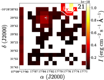
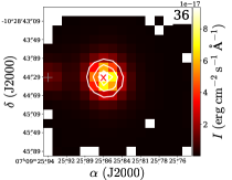
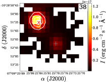
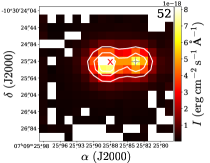
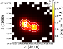
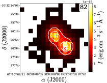
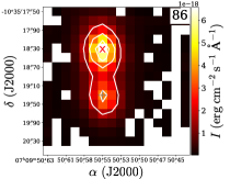
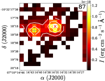
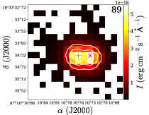
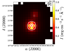
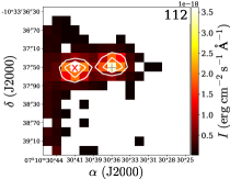
Figure 2: KMOS $K$-band continuum maps of YSO candidates with possible stellar companions. Only spaxels with the continuum flux above 3$\sigma$ are shown. White contours correspond to 25%, 50%, and 75% of the $K$-band continuum peak. The position of the brighter source in each map is indicated with a red ’$\times$’ symbol (the “A” component in Table 2), and the fainter one with a grey ’$+$’ symbol (the “B” component). The size of the pixel (0.2$\arcsec$) corresponds to 184 au.

3 Data Analysis and Results

Out of 118 Spitzer YSO candidates observed with KMOS, 5 were not detected and 11 were resolved into two near-IR sources. In total, our KMOS observations provide the $K$-band data for 124 sources.

The IFU observations deliver both the spectral and spatial information. The $K$-band continuum emission allows us to identify all the continuum components and determine their positions and $K$-band fluxes. The spatial extent of the atomic and molecular emission hints at the underlying physical mechanisms and their characteristics. The hydrogen Br$\gamma$ emission is correlated with the UV continuum excess diagnostic of mass accretion. The CO ro-vibrational band head traces the inner disk. The H₂ emission lines, including the bright 1-0 S(1) line at 2.12 $\mu$m, trace jets and shocks.

In this section, we discuss the spatial distribution of gas and dust, and summarize the line detections and kinematic information.

3.1 $K$-Band Continuum Emission

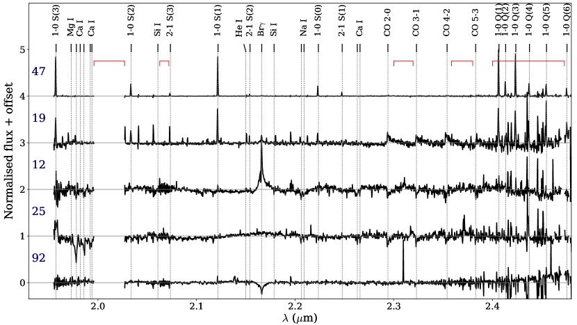
Figure 3: Example spectra of YSOs in CMa-$\ell$224. Source names from Table 2 (No.) are provided on the left side of the respective spectra. All spectra are normalised to the continuum peak flux density in the wavelength range from 1.97 to 2.47 $\mu$m. The red horizontal lines show spectral ranges most affected by telluric lines; the wavelength range around 2.0 $\mu$m has been removed for clarity of the plot.

All the $K$-band continuum sources detected with VLT/KMOS in CMa-$\ell$224 are listed in Table 2. The table provides the sources’ GLIMPSE360 catalog names and assigned KMOS IDs, their equatorial coordinates corresponding to the position of the $K$-band continuum peak, the $K$-band continuum fluxes estimated near 2.12 $\mu$m, the YSO classification from Sewiło et al. (2019), and remarks on pointing, multiplicity, and the association with extended H₂ emission. Two $K$-band continuum components have been detected toward eleven fields centered on single Spitzer YSO candidates (see Fig. 2); the brighter source is listed in Table 2 as source “A” and the fainter one as source “B.”

Selected $K$-band continuum maps are shown in Figure 2 (11 fields with the detection of two sources) and Appendix A (the remaining fields).

We consider a possibility that two sources detected in a single KMOS field are two components of a binary star/YSO. The median separation between the two components of the “binary star candidates” in CMa-$\ell$224 is 760 au (see Table 2), with a range from 370 au (source No. 89) to 1180 au (source No. 38). All but three pairs of visual binary star candidates have spectra typical of accreting young stars: emission of Br$\gamma$ and/or H₂. Two more pairs have CO bandhead in absorption typical for cool stars. Given the proximity of the sources, they may be physically related. If they are binary systems, the multiplicity fraction defined as the ratio of the number of multiple systems to the total number of systems (both single and multiple), is $0.09\pm 0.01$. For comparison, the multiplicity fraction for separations between 100 and 1000 au is $0.15\pm 0.04$ for protostars in Perseus (Tobin et al., 2016), $0.14\pm 0.01$ for protostars and $0.13\pm 0.01$ for Pre-Main Sequence (PMS) stars in the Orion molecular clouds (Kounkel et al., 2016). Adopting the approximate range recovered by KMOS (180-1180 au), the multiplicity fraction of protostars would be $\sim$0.09 in Perseus and 0.12 in Orion.

In summary, the binary star candidates in CMa-$\ell$224 have the multiplicity fraction that is consistent with YSOs in other molecular clouds, once we account for close binaries that are unresolved with KMOS. A more robust comparison requires an unbiased survey of YSOs at their earliest evolutionary stages and will be presented in the second paper in this series.

3.2 Spectral Line Detections

KMOS spectra contain several atomic and molecular lines emerging as a result of mass accretion and/or ejection in YSOs. Additionally, transitions of many atomic absorption lines which originate from a stellar photosphere are also detected and can be used to estimate spectral types and luminosity classes of YSOs (e.g., Nisini et al., 2005; Luhman & Rieke, 1998).

Figure 3 shows the $K$-band spectra toward selected YSO candidates with diverse characteristics to illustrate the differences between the sources. For example, sources No. 47 and 19 show a strong H₂ emission, with only the latter showing also clear Br$\gamma$ and CO detections. Sources No. 12 and 25 both show CO bandhead in absorption. Yet, only source No. 12 is characterized also by a broad emission line profile in Br$\gamma$. Source No. 92 shows very weak H₂ emission, and Br$\gamma$ line in absorption. The line detections are discussed further in the subsequent sections.

3.2.1 Br$\gamma$

The most commonly detected line is the 2.1655 $\mu$m Br$\gamma$ hydrogen line, seen in emission in 58 sources (47%) and in absorption in 16 sources (13%). Twenty six sources with the Br$\gamma$ emission also show the CO lines in absorption. A similar pattern but higher detection rates of the Br$\gamma$ emission ($\sim 75$%), was found toward a sample of 19 Class I protostars (Connelley & Greene, 2010, 2014). In a recent KMOS survey of YSOs in Perseus, the Br$\gamma$ was indeed more commonly detected in emission toward Class I (59%) than Class II YSOs (36%, Fiorellino et al., 2021).

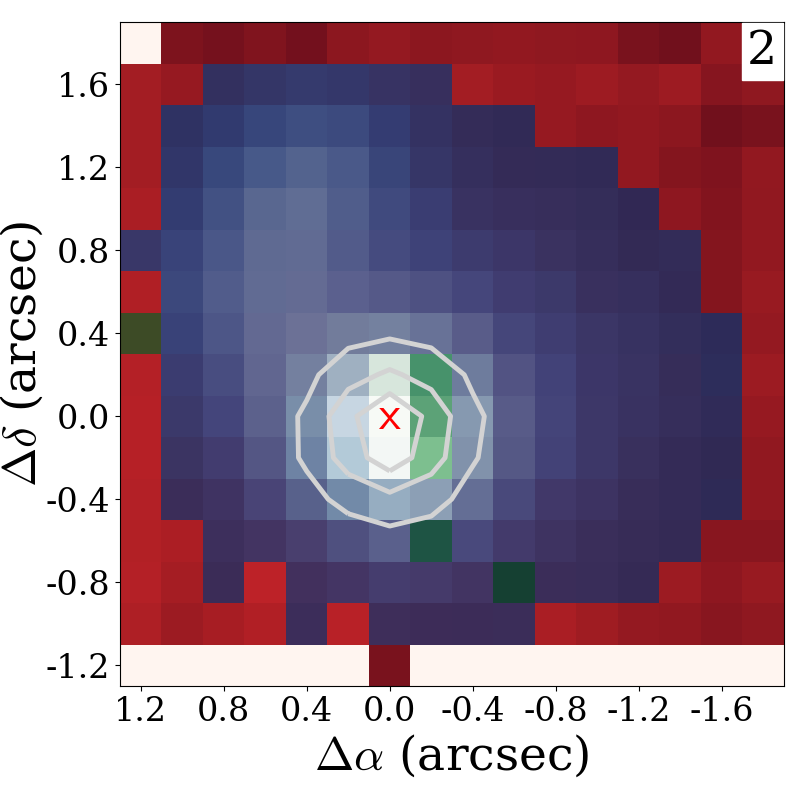
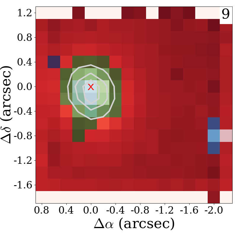
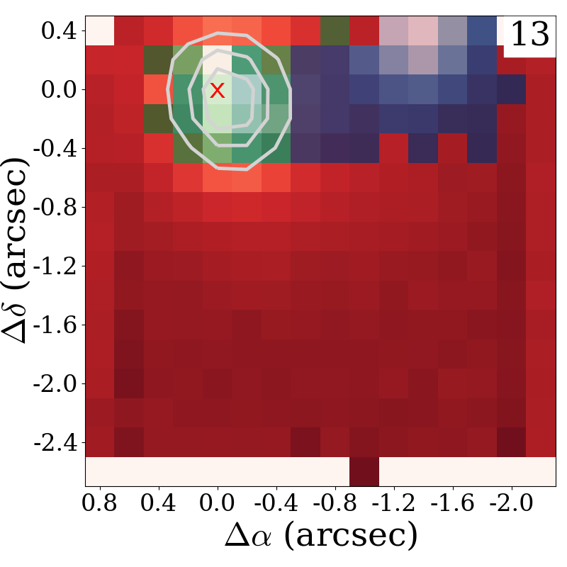
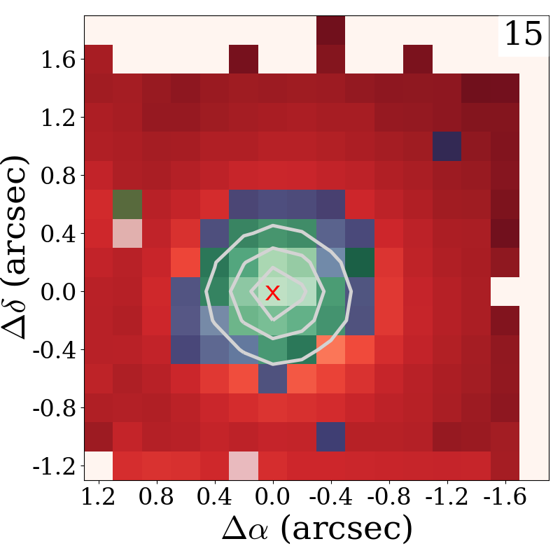
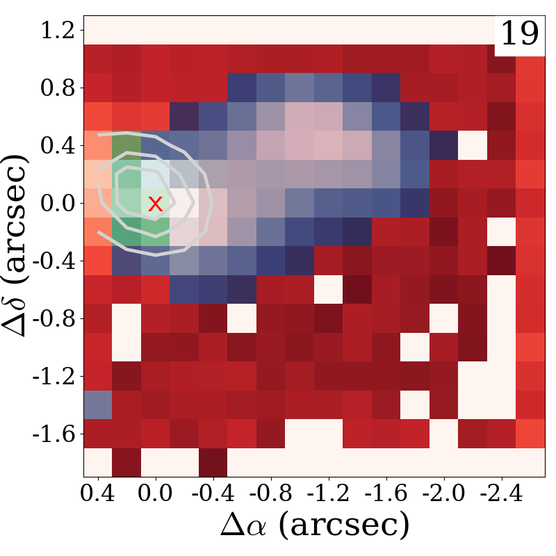
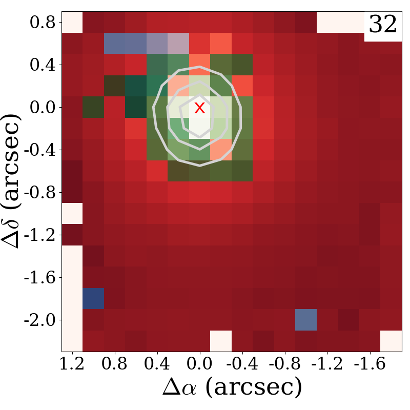
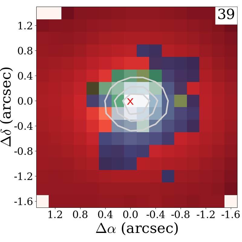
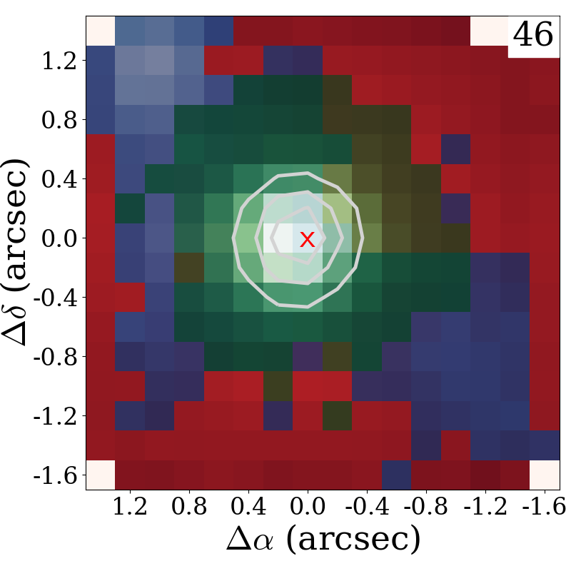
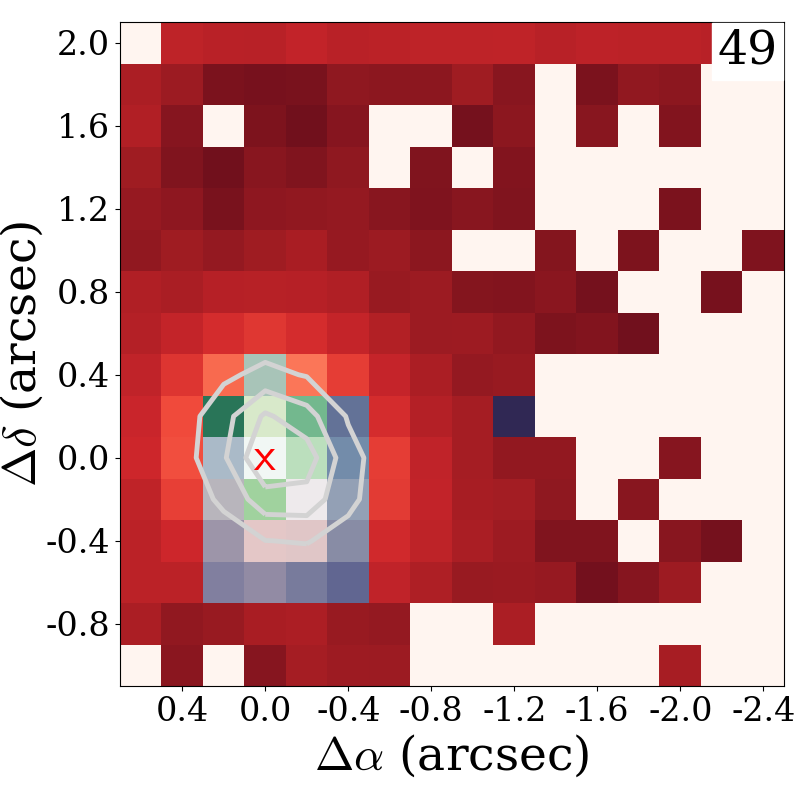
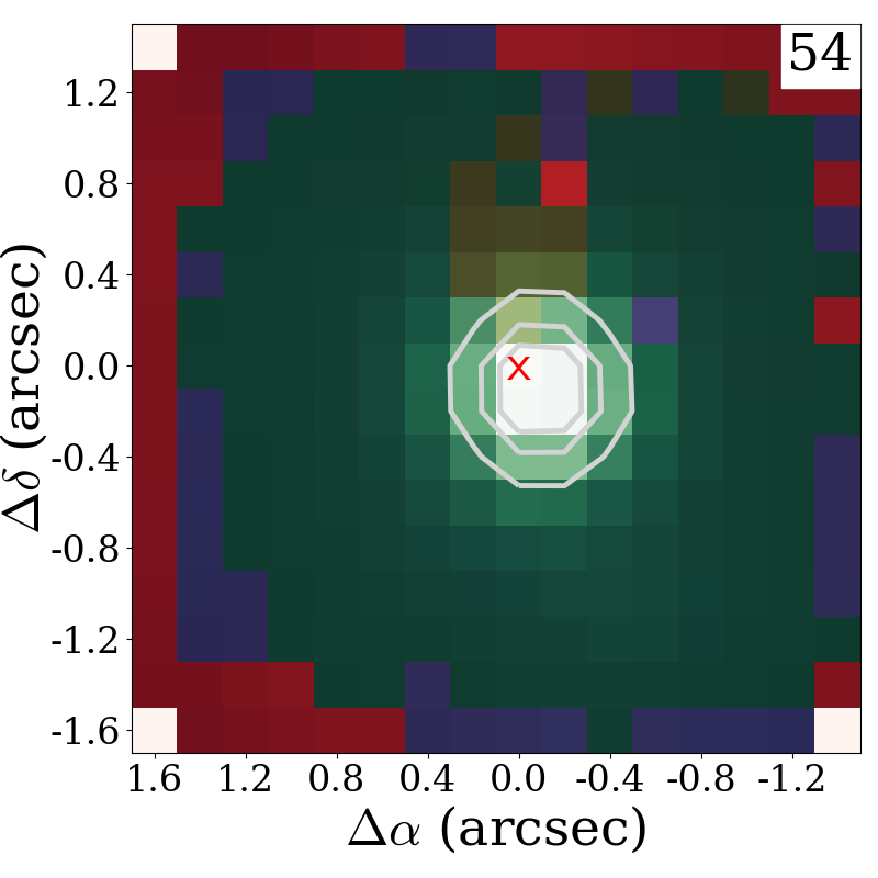
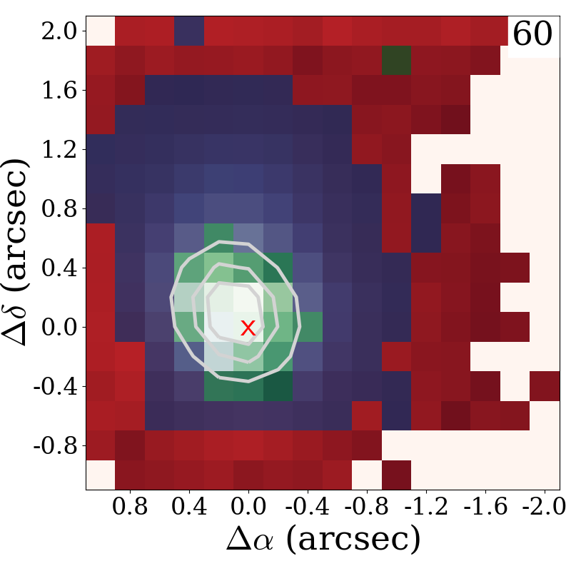
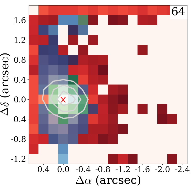
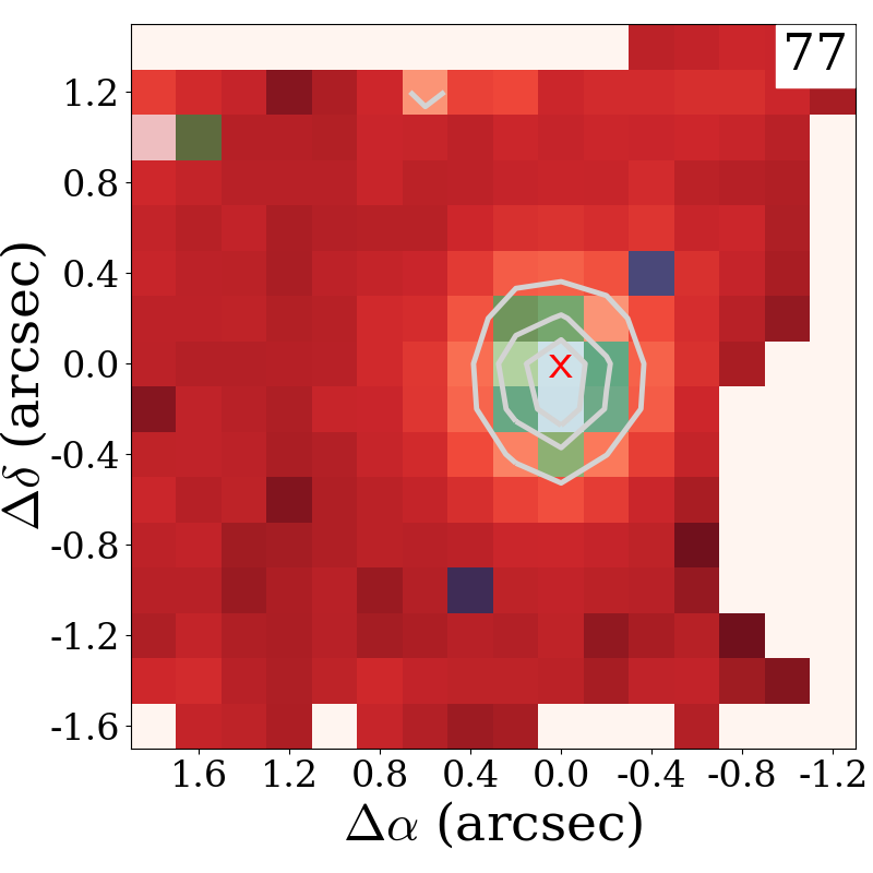
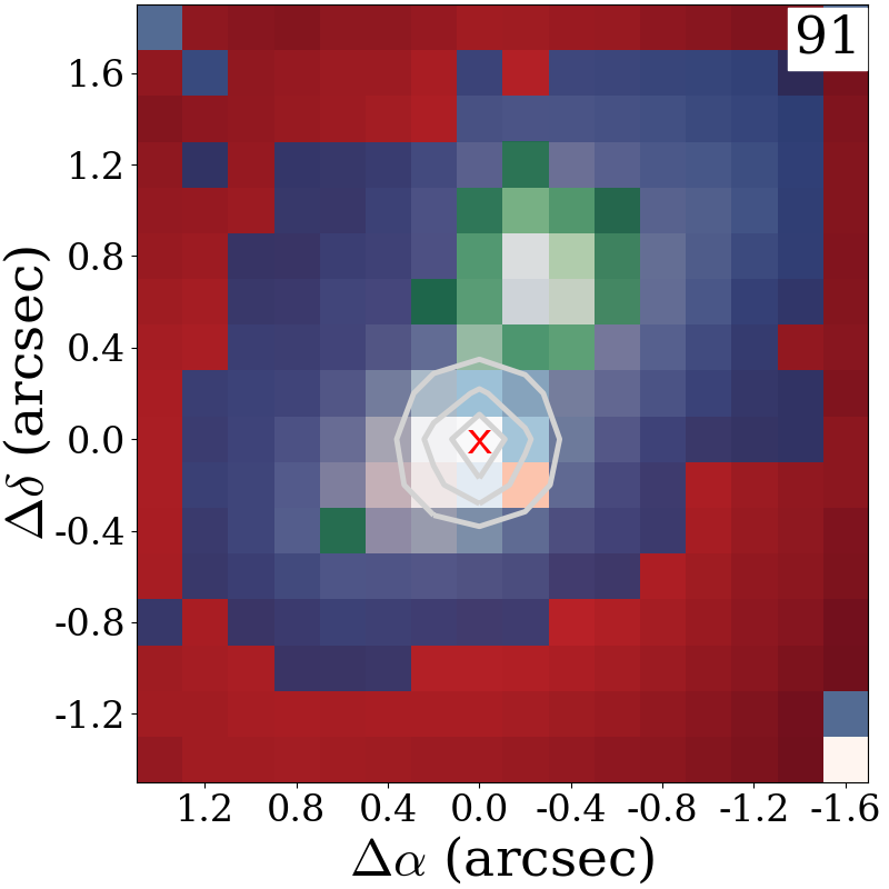
Figure 4: Three-color composite images of YSO candidates with the $\geq$3$\sigma$ detection in the H₂ line at 2.12 $\mu$m (in blue), Br$\gamma$ line at 2.17 $\mu$m (in green), and the $K$-band continuum (in red). In each image, white contours correspond to the $K$-band continuum emission with contour levels of 25%, 50%, and 75% of the continuum peak marked with the red ’$\times$’ symbol. Source IDs are indicated in the upper right corners.

The Br$\gamma$ line emission in our sources is compact and associated with the continuum emission (Section 3.1, see also Fig. 4 and Appendix C). In low-mass YSOs, Br$\gamma$ emission originates from the close vicinity of the young star and usually traces magnetospheric accretion columns, with possible contributions from winds (Kraus et al., 2008). Some emission may also arise along the outflows (Beck et al., 2010).

The spatial extent of atomic emission of Br$\gamma$-emitting gas is often more compact than molecular gas, with the exception of source No. 54, a bright star with the $K$-band magnitude of 9.9 (Fig. 4). Extended emission around a young star can be partially explained by an emerging H II region, but a broad line profile suggests that other physical processes might also contribute (Cooper et al., 2013). The physical extent of $\sim$2350 au of Br_γ emission from the source No. 54 cannot be explained with disk winds. In the subsequent analysis, the line fluxes are extracted from the area covering the continuum source, where Br$\gamma$ emission is likely dominated by accretion.

3.2.2 H₂

H₂ is a homonuclear molecule that lacks a permanent dipole moment, thus only quadrupole transitions may occur ($\Delta J=0,\pm 2$). The extended distribution of the H₂ emission and its velocity structure indicate the origin in bipolar outflows (Section 3.4). H₂ emission is detected in 33 sources in CMa-$\ell$224 (27%), including 14 that also show a detection of the Br$\gamma$ line in emission, and only 3 with the CO ro-vibrational lines in absorption. A similar H₂ detection rate of 23% was reported in a pioneering survey of Carr (1990). Larger rates have been found toward Class I protostars (43%, Connelley & Greene, 2014) and higher-mass YSOs (56%, Cooper et al. 2013; 76%, Varricatt et al. 2010). Line fluxes are reported in Appendix B in Table 5.

3.2.3 CO

The CO bandhead in absorption traces the atmosphere of a star or a disk. Among YSO candidates in CMa-$\ell$224, the CO first overtone is detected in absorption in 60% of YSO candidates, predominately (78%) in those classified as Class II (Sewiło et al., 2019, see also Table 2). Among Class I YSOs, the CO absorption is detected in 43% of the sources, similar to the 57% detection rate in Connelley & Greene (2010), and $>$2.5 times more than in the Cooper et al. (2013) survey.

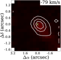
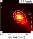
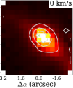
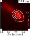
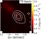
Figure 5: The H₂ 1-0 S(1) channel maps for source No. 47. The velocities relative to the rest velocity of the H₂ line are shown in the upper right corners. The green ’$\times$‘ symbol shows the position of the $K$-band continuum peak.

The CO bandhead in emission indicates high accretion rates onto the YSO disk, possibly also associated with an accretion burst (e.g., Lorenzetti et al., 2009; Guo et al., 2021). The CO bandhead emission requires high temperatures ($2500-4000$ K) and densities ($n_{\rm{H}}>10^{10}$ cm^-3) to excite the upper levels (e.g., Carr, 1989; Casali & Eiroa, 1996). In CMa-$\ell$224, only 5% of the sources detected with KMOS show the CO bandhead in emission (4 Class I and 2 Class II YSOs). This detection rate is a factor of 4-5 lower than in the Carr (1989) and Connelley & Greene (2010) surveys, likely due their focus on Class I protostars. All of our sources with the CO bandhead emission also show the H₂ and Br$\gamma$ emission, and in four out of six sources the H₂ emission is extended, suggesting intensive mass accretion and subsequent ejection.

3.2.4 Other Lines

Spectra of eleven YSO candidates show multiple atomic lines e.g., He I, Mg I, Ca I, Na I, K I, or Si I typical for late spectral types (K–M, Nisini et al., 2005); however, they do not reveal the presence of the Br$\gamma$, H₂, and CO lines. The confirmation of their YSO status would require careful spectral typing and further analysis, which will be presented in the future work in this series. Appendix B shows spectra of all those sources and the information about the detection of the key spectral lines.

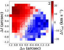
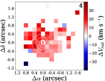
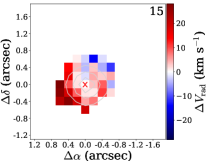
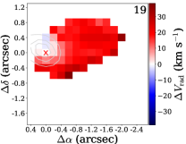
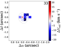
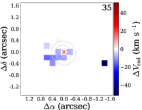
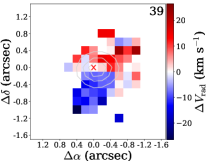
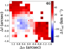
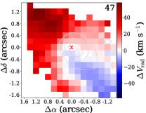
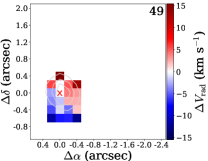
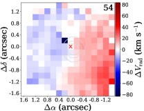
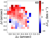
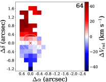
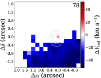
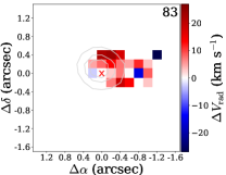
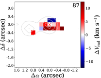
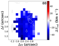
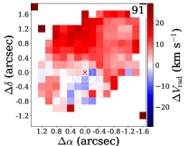
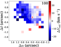
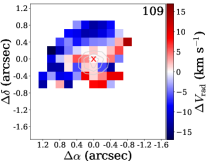
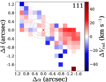
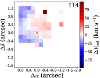
Figure 6: The H₂ 1-0 S(1) velocity centroid maps for all YSOs associated with the H₂ emission; the velocities are calculated with respect to the radial velocity of the corresponding source. Only pixels with the H₂ detection above 3$\sigma$ are shown. The contours show the $K$-band continuum emission, and the red crosses the positions of the YSO candidates (the peak of the $K$-band continuum emission). The source names are indicated in the upper right corners. Radial velocities of the gas associated with sources No. 78 and 88 cannot be estimated, and here only the apparent radial velocities are shown. The KMOS spectral sampling at 2.12 $\mu$m corresponds to 39.67 km/s.

3.3 Extinction

The line fluxes in the near-IR are affected by extinction. We adopt $A_{\rm{V}}$ obtained from the spectral energy distribution (SED) modelling by Sewiło et al. (2019) for 85 sources in our sample. Our $K$-band observations cover several H₂ lines that are often used to estimate $A_{\rm{V}}$; however, after assessing the quality of our H₂ data, we decided against using this method due to the small separation between the two lines ($\sim 0.2$ $\mu$m), uncertainty in telluric corrections near the Q-branch H₂ emission, and small number of sources for which this method can be used.

We assess the uncertainty of extinction estimated from the SED fitting using the work by Furlan et al. (2016). There, the R statistics was used to calculate a mode – the value with the highest frequency within a certain range from the best-fit R value (see their Fig. 48). Almost all their $A_{\rm{V}}$ uncertainties are consistent with a 1:1 correlation within a 10 mag error. We adopt this conservative value in the subsequent analysis, in particular in the calculation of the mass accretion (Sections 3.5).

We note that extinction is expected to differ between the position of the infrared continuum source and the outflow (Yoon et al., 2022). The ratios of the hydrogen Br$\gamma$ and Pa$\alpha$ lines are routinely used to estimate $A_{\rm{V}}$ toward the accretion region (Fiorellino et al., 2021), but the latter line is located in the $H$-band and not covered by our observations. Since SED modelling provides the estimate of $A_{\rm{V}}$ toward the central star and H₂ emission is often extended, such $A_{\rm{V}}$ estimate is likely not representative for the true reddening of the H₂ lines. Therefore, we do not apply it for those lines. Thus, Table 5 shows the H₂ line fluxes, which are not corrected for extinction.

3.4 Gas Spatial Distribution and Kinematics

The spatial distribution of the line emission varies significantly between different species detected with KMOS (Fig. 4). The Br$\gamma$ emission is spatially unresolved for the majority of the sources, in line with the origin in the inner disk. Similarly, the CO bandhead emission is also compact and co-spatial with the continuum emission. In contrast to the Br$\gamma$ and CO bandhead emission, the H₂ emission is usually extended.

The extended distribution of the H₂ emission resembles the structure of the molecular outflows from Class 0/I protostars for 14 out of 33 sources with the H₂ line detection (42% or 11% of the entire sample; see Fig. 4). In five sources, the extended H₂ emission is not associated with the targeted source (see Table 2) and likely originates from an outflow from another YSO. Those five cases often show only one lobe within the field of view. Among other sources with the detection of H₂, the emission pattern does not show two prominent outflow lobes. The lack of the bipolar pattern might be due to too low spatial resolution or the projection effects. In general, a contribution from a photo-dissociation region is unlikely among the low-mass YSOs found in CMa-$\ell$224. The emission maps for the Br$\gamma$, H₂, and CO bandhead lines for the entire KMOS YSO sample in CMa-$\ell$224 are presented in Appendix C.

We use the brightest and spectroscopically well-resolved H₂ line in $K$-band, the 1-0 S(1) transition at 2.12 $\mu$m, to calculate radial velocities of the emitting gas. Figure 5 shows selected channel maps for an example source (No. 47) associated with an extended H₂ emission. Here, the blue-shifted emission transitions into red-shifted one on the other side of the central source, which is a clear signature of a bipolar ejection. The images reveal a velocity structure consistent with an outflow with velocities up to 50 km s^-1. A similar kinematic structure has been detected toward most of the other sources with the extended H₂ emission (No. 2, 15, 19, 46, 47, 54, 60, 64, 91 and 114; see Figure 6). The large spatial scales of those structures cannot be due to the emission from protoplanetary disks since they are too cold at such large distances from the central star to excite H₂.

The H₂ emission structure associated with sources No. 78 and 88 resembles the single outflow lobes; however, the continuum source is not seen in the map of the YSO candidate No. 88, while for No. 78, the H₂ emission does not seem to be physically connected to the source. Additional observations with a larger field-of-view are needed to identify sources responsible for the extended H₂ emission in these fields.

The estimated relative velocities do not exceed $\sim$50 km/s, with velocities increasing towards lobe ends, typical for outflow-driven shock waves. The moderate spectral resolution of KMOS does not allow for a detailed study on outflow kinematics, including any minor variations in kinematic patterns. The spatial extent of the H₂ gas supports the origin in outflow shocks. The limited wavelength coverage of our spectra, however, does not allow to properly estimate extinction as a function of position along the outflow (see Section 3.3).

Finally, we note that the bipolar structure in several H₂ lines toward source No. 47 (Appendix C) is consistent with its classification as a Class I source using SED models (Sewiło et al., 2019). The prominent H₂ outflow suggest that the source might be one of the youngest in our sample. It would be a suitable candidate for a detailed spectral modeling using shock models; however, this is outside of the scope of this paper.

3.5 Gas Accretion

Gas accretion onto Class II YSOs is typically measured using UV continuum excess or line emission in e.g., H, He or Ca II at optical wavelengths (e.g., Alcalá et al., 2014; Nisini et al., 2018). In more embedded Class I YSOs, the accretion is more often quantified using hydrogen lines in the near-IR which are less affected by dust extinction (Muzerolle et al., 1998; Natta et al., 2004).

We estimate the accretion luminosity ($L_{\mathrm{acc}}$ in units of L_⊙) for YSOs in CMa-$\ell$224 by measuring the flux of the hydrogen Br$\gamma$ line. As illustrated in Figure 3, the Br$\gamma$ emission arises from the same area as the continuum source; we therefore assume it traces primarily the unresolved accretion region (see also Section 3.2.1). We use the relation between $L_{\mathrm{Br}\gamma}$ and $L_{\mathrm{acc}}$ for low- and intermediate-mass YSOs from (Alcalá et al., 2017) to estimate $L_{\mathrm{acc}}$:

$$\log{(L_{acc})}=(1.19\pm 0.10)\cdot\log{L_{Br\gamma}}+(4.02\pm 0.51)$$ (1)

The mass accretion rates, $\dot{M}_{acc}$, are then calculated using the formula:

$$\dot{M}_{acc}=L_{acc}\times\left(1-\frac{R_{*}}{R_{\mathrm{in}}}\right)^{-1}\frac{R_{*}}{GM_{*}}$$ (2)

where $R_{*}$ and $M_{*}$ are the stellar radius and mass, respectively, and $R_{\mathrm{in}}$ is the inner-disk radius; typically $R_{\mathrm{in}}$ is assumed to equal 5$R_{*}$ (Gullbring et al., 1998). Although the relation was found for Class II objects, it is a specific case of the general formula describing efficiency of converting kinetic energy of falling matter onto a stellar photosphere into radiation and can be applied to Class I sources as well (see the review of Hartmann et al. 2016 or a recent paper of Fiorellino et al. 2022).

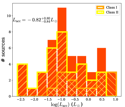
Figure 7: Histogram of the accretion luminosities ($L_{\mathrm{acc}}$) based on Br$\gamma$ line luminosity (Table 3) measured toward YSOs in CMa-$\ell$224 (in dark orange). The median value of $L_{\mathrm{acc}}$ is indicated at the top of the plot. The orange and yellow hatched histograms show the distribution of $L_{\mathrm{acc}}$ for sources classified by Sewiło et al. (2019) as, respectively, Class I and Class II YSO candidates.

To calculate the mass accretion rates, knowledge of stellar masses and radii is needed. Stellar parameters for 17 sources from our sample have been estimated from the SED fitting (Sewiło et al., 2019); only half of them are associated with the Br$\gamma$ emission. The typical masses are $\sim 2~{}M_{\odot}$ and radii are $\sim 3~{}R_{\odot}$. The median logarithm of the accretion luminosity is -0.82${}_{-0.84}^{+0.80}$  $L_{\odot}$ and the median logarithm of the accretion rate is -7.92${}^{+1.06}_{-1.09}$  M_⊙yr^-1 for sources with $A_{V}$ estimates.

Table 3: Accretion properties of YSOs in CMa-$\ell$224.

No.	Br$\gamma$	$\log{(L_{\rm{acc}})}$	$\log{(\dot{M}_{\mathrm{acc}})}$
	10-16 (erg s-1 cm-2)	(L⊙)	(M⊙yr-1)
2	13.00 $\pm$ 0.32	-1.30${}_{-0.82}^{+0.76}$	$\cdots$
3	13.89 $\pm$ 0.32	-1.26${}_{-0.73}^{+0.72}$	$\cdots$
5	-397.29 $\pm$ 0.55	$\cdots$	$\cdots$
6	19.08 $\pm$ 0.25	-1.09${}_{-0.81}^{+0.79}$	$\cdots$
9	341.80 $\pm$ 0.79	0.40${}_{-0.86}^{+0.86}$	$\cdots$
10	54.74 $\pm$ 0.45	-0.55${}_{-0.86}^{+0.84}$	$\cdots$
12	352.30 $\pm$ 1.35	0.41${}_{-0.90}^{+0.89}$	$\cdots$
13	28.33 $\pm$ 0.77	-0.89${}_{-0.80}^{+0.79}$	$\cdots$
15	521.01 $\pm$ 0.35	0.62${}_{-0.88}^{+0.87}$	$\cdots$
16	108.77 $\pm$ 1.57	-0.19${}_{-0.87}^{+0.85}$	-7.50${}_{-1.07}^{+1.05}$
18*	1.52 $\pm$ 0.34	-2.40${}_{-0.10}^{+0.08}$	$\cdots$
19	68.62 $\pm$ 0.21	-0.43${}_{-0.84}^{+0.83}$	$\cdots$
20	12.93 $\pm$ 0.85	-1.29${}_{-0.84}^{+0.80}$	$\cdots$
22*	1.63 $\pm$ 0.56	-2.36${}_{-0.19}^{+0.13}$	$\cdots$
23*	4.91 $\pm$ 1.36	-1.79${}_{-0.19}^{+0.15}$	$\cdots$
24	100.01 $\pm$ 0.29	-0.24${}_{-0.80}^{+0.80}$	$\cdots$
26	18.52 $\pm$ 0.33	-1.11${}_{-0.93}^{+0.85}$	$\cdots$
28	33.00 $\pm$ 0.60	-0.81${}_{-0.75}^{+0.74}$	$\cdots$
30	1.00 $\pm$ 0.20	-2.62${}_{-0.74}^{+0.69}$	$\cdots$
31*	1.16 $\pm$ 0.16	-2.54${}_{-0.03}^{+0.02}$	$\cdots$
32	27.83 $\pm$ 3.14	-0.90${}_{-0.86}^{+0.82}$	$\cdots$
33	17.17 $\pm$ 0.31	-1.15${}_{-0.82}^{+0.80}$	$\cdots$
34*	4.82 $\pm$ 0.34	-1.80${}_{-0.06}^{+0.06}$	$\cdots$
35	-20.72 $\pm$ 0.54	$\cdots$	$\cdots$
36A*	65.58 $\pm$ 2.41	-0.46${}_{-0.15}^{+0.15}$	-7.69${}_{-0.35}^{+0.35}$
38A*	2.36 $\pm$ 0.35	-2.17${}_{-0.07}^{+0.06}$	$\cdots$
38B*	0.36 $\pm$ 0.09	-3.15${}_{-0.06}^{+0.03}$	$\cdots$
39	33.48 $\pm$ 3.62	-0.80${}_{-0.95}^{+0.88}$	-8.10${}_{-1.15}^{+1.08}$
40	-2119.07 $\pm$ 12.85	$\cdots$	$\cdots$
41*	10.11 $\pm$ 0.59	-1.42${}_{-0.08}^{+0.08}$	$\cdots$
43	-1.29 $\pm$ 0.27	$\cdots$	$\cdots$
45	4.54 $\pm$ 0.27	-1.83${}_{-1.09}^{+0.87}$	$\cdots$
46	307.57 $\pm$ 5.92	0.34${}_{-0.87}^{+0.86}$	-6.97${}_{-1.07}^{+1.06}$
47	373.10 $\pm$ 0.37	0.44${}_{-0.89}^{+0.86}$	$\cdots$
48	1.37 $\pm$ 0.33	-2.45${}_{-0.80}^{+0.73}$	$\cdots$
49	119.13 $\pm$ 0.60	-0.15${}_{-0.90}^{+0.87}$	$\cdots$
50	94.51 $\pm$ 0.52	-0.27${}_{-0.78}^{+0.78}$	$\cdots$
52A*	2.38 $\pm$ 0.45	-2.17${}_{-0.10}^{+0.08}$	$\cdots$
52B*	1.56 $\pm$ 0.50	-2.39${}_{-0.17}^{+0.12}$	$\cdots$
53	-107.15 $\pm$ 0.76	$\cdots$	$\cdots$
54*	493.43 $\pm$ 19.10	0.59${}_{-0.24}^{+0.24}$	$\cdots$
55A	9.30 $\pm$ 1.35	-1.46${}_{-0.79}^{+0.76}$	-8.41${}_{-0.99}^{+0.96}$
56	19.69 $\pm$ 0.40	-1.08${}_{-0.86}^{+0.82}$	$\cdots$
57*	3.87 $\pm$ 0.93	-1.92${}_{-0.15}^{+0.12}$	$\cdots$
58	7.93 $\pm$ 1.03	-1.55${}_{-0.79}^{+0.76}$	$\cdots$
60	1163.21 $\pm$ 1.90	1.03${}_{-0.87}^{+0.85}$	$\cdots$
61	-3.22 $\pm$ 0.45	$\cdots$	$\cdots$
63	-34.89 $\pm$ 0.53	$\cdots$	$\cdots$
64	413.58 $\pm$ 0.40	0.50${}_{-0.71}^{+0.71}$	$\cdots$
68	2.63 $\pm$ 0.39	-2.12${}_{-0.83}^{+0.76}$	$\cdots$
71	-69.23 $\pm$ 0.25	$\cdots$	$\cdots$
72*	1.66 $\pm$ 0.58	-2.36${}_{-0.20}^{+0.13}$	$\cdots$
73	44.53 $\pm$ 0.30	-0.66${}_{-0.81}^{+0.80}$	$\cdots$
75	-58.02 $\pm$ 0.27	$\cdots$	$\cdots$
76	30.09 $\pm$ 0.38	-0.86${}_{-0.84}^{+0.81}$	$\cdots$
77	276.96 $\pm$ 0.21	0.29${}_{-0.85}^{+0.85}$	$\cdots$
79	9.33 $\pm$ 0.31	-1.46${}_{-0.77}^{+0.75}$	-8.48${}_{-0.97}^{+0.95}$
80*	2.65 $\pm$ 0.73	-2.11${}_{-0.16}^{+0.12}$	$\cdots$
81	65.21 $\pm$ 0.82	-0.46${}_{-0.90}^{+0.87}$	-7.74${}_{-1.10}^{+1.07}$
83	625.84 $\pm$ 0.35	0.71${}_{-0.84}^{+0.78}$	$\cdots$
84	-109.85 $\pm$ 0.87	$\cdots$	$\cdots$
85*	8.34 $\pm$ 0.50	-1.52${}_{-0.08}^{+0.07}$	$\cdots$
86B	1.10 $\pm$ 0.14	-2.57${}_{-0.72}^{+0.68}$	$\cdots$
89A*	0.81 $\pm$ 0.23	-2.72${}_{-0.12}^{+0.07}$	$\cdots$
89B*	0.24 $\pm$ 0.08	-3.36${}_{-0.10}^{+0.04}$	$\cdots$
91A*	-6.12 $\pm$ 1.11	$\cdots$	$\cdots$
91B*	6.90 $\pm$ 0.50	-1.62${}_{-0.08}^{+0.07}$	$\cdots$
92	-14.75 $\pm$ 0.51	$\cdots$	$\cdots$
93	115.79 $\pm$ 0.52	-0.16${}_{-0.84}^{+0.83}$	$\cdots$
94	-3.35 $\pm$ 0.25	$\cdots$	$\cdots$
96	-56.89 $\pm$ 0.71	$\cdots$	$\cdots$
97	29.29 $\pm$ 1.65	-0.87${}_{-0.89}^{+0.84}$	$\cdots$
98	4.91 $\pm$ 0.42	-1.80${}_{-0.75}^{+0.73}$	$\cdots$
99*	1.42 $\pm$ 0.25	-2.44${}_{-0.07}^{+0.05}$	$\cdots$
102	273.94 $\pm$ 3.28	0.28${}_{-0.85}^{+0.84}$	$\cdots$
104	-6.90 $\pm$ 0.81	$\cdots$	$\cdots$
109	716.77 $\pm$ 0.24	0.78${}_{-0.73}^{+0.73}$	$\cdots$
111	51.99 $\pm$ 0.37	-0.58${}_{-0.76}^{+0.76}$	$\cdots$
112A	9.55 $\pm$ 0.16	-1.45${}_{-0.72}^{+0.71}$	$\cdots$
112B	30.86 $\pm$ 0.14	-0.84${}_{-0.76}^{+0.76}$	$\cdots$
114	187.72 $\pm$ 0.76	0.09${}_{-1.08}^{+0.97}$	-7.06${}_{-1.28}^{+1.17}$
116	-3.91 $\pm$ 0.28	$\cdots$	$\cdots$
117	-4.64 $\pm$ 0.51	$\cdots$	$\cdots$
118	9.01 $\pm$ 0.43	-1.48${}_{-0.78}^{+0.76}$	$\cdots$

Note. — Negative flux values indicate absorption. Measurements for targets with asterisk have not been corrected for extinction. Flux uncertainties do not cover the extinction uncertainty of 10 mag, which is included in uncertainties of accretion luminosity and mass accretion rates. Uncertainties of $\log{(L_{\mathrm{acc}})}$ and $\log{(\dot{M}_{\mathrm{acc}})}$ do not include the systematic distance uncertainty.

All accretion luminosities and, where available, mass accretion rates and associated uncertainties are listed in Table 3. The uncertainties of mass accretion rates account for the uncertainties in line fluxes, $L_{\rm Br\gamma}$–$L_{\rm acc}$ relation, extinction ($A_{\mathrm{V}}$ of 10 mag, corresponding to $\sim$1 mag in $K$-band), and 0.1 dex for both M_∗ and R_∗. We do not include, however, the uncertainty of the distance to the region, which is systematic. The adopted value of 0.92 kpc from Sewiło et al. (2019) is consistent with those from stellar studies (1.05$\pm$0.15 kpc, 0.99$\pm$0.05 kpc, 1.15$\pm$0.06 kpc, Shevchenko et al., 1999; Kaltcheva & Hilditch, 2000; Lombardi et al., 2011, respectively), and recent estimates using ALMA observations (a median of 0.92 kpc for cores within our pointings, Olmi et al., 2023).

We also cross-checked the distance to CMa-l224 with the results from the 3D dust maps using photometry from Pan-STARRS 1 and 2MASS, as well as the Gaia parallaxes (Green et al., 2019). The median distance estimated this way for several targets in our study yields 1.26 kpc. The value exceeds our adopted distance of 0.92 kpc, with the difference that is larger than uncertainties of previous studies and the dispersion of individual distance values. Thus, we consider 0.34 kpc as the uncertainty of the distance; it corresponds to the uncertainty of 0.27 dex in accretion luminosity and mass accretion rate.

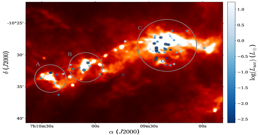
Figure 8: Distribution of accretion luminosity in the main filament in CMa-$\ell$224 (blue color scale). Class I sources are marked with hexagon and Class II sources with star symbols. Black circles mark targets without $A_{\rm{V}}$ estimation. Marked with grey circles are three regions identified by Sewiło et al. (2019).

Figure 7 shows the distribution of accretion luminosities among Class I and II YSOs, which range from -2.5 to 0.6 $L_{\odot}$ in logarithm. The distributions of $L_{\mathrm{acc}}$ are similar for both Class I and II YSOs, but the number of Class II YSOs in this sample is two times higher than Class I YSOs. We do not find any correlation between accretion luminosity and stellar mass, but the number of mass measurements is too small and the mass measurements are too uncertain to draw reliable conclusions. Accretion rate estimations are feasible only for 8 Class II YSOs (including one binary candidate), with available mass and radius estimates; their logarithmic values range from -8.4 to -7.0  M_⊙yr^-1.

4 Discussion

4.1 Star Formation in CMa-$\ell$224

Star formation in Canis Majoris is closely linked with a supernova explosion $\sim$1.5 Myr ago (Herbst & Assousa, 1977; Comeron et al., 1998). The expanding shell, coincident with CMa-$\ell$224, might have compressed the interstellar medium in a turbulent flow and triggered the filament formation (Fischer et al., 2016; Sewiło et al., 2019). The main filament in the region is highly supercritical (Olmi et al., 2016), which leads to gravitational fragmentation and the formation of clumps and cores (André, 2017). Overall, the filament is associated with $\sim$700 starless cores and $\sim$250 prestellar cores (Elia et al., 2013), and the largest concentration of Class I YSOs in the entire Canis Major star-forming region (Fischer et al., 2016; Sewiło et al., 2019).

Integral Field Spectroscopy in $K$-band at high-angular resolution provides unique insights into star formation processes on scales of individual YSOs in the main filament of CMa-$\ell$224. As shown in Section 3, the compact emission in the Br$\gamma$ line traces the on-going accretion onto the young stars, whereas the spatial distribution and kinematics of H₂ pin-points molecular outflows and mass ejection. The question remains, to what extent the mass accretion and ejections rates in YSOs are linked with the properties of the filament and its possible evolution.

Figure 8 shows the distribution of accretion luminosity in the main filament in CMa-$\ell$224 (Section 3.5). YSOs are preferentially located within three “clusters” associated with bright far-IR continuum emission. Following the nomenclature introduced in Sewiło et al. (2019), cluster C is known to coincide also with C¹⁸O 2-1 emission and the peak of ¹³CO 1-0, with the latter encompassing the entire filament (Olmi et al., 2016). The ¹³CO and C¹⁸O line observations revealed a velocity gradient along the main filament, which extends from cluster C to A (Olmi et al., 2016) and is likely responsible for the formation of YSOs at the ridge connecting clusters B and C. Another velocity gradient was identified from a secondary filament which is roughly perpendicular to the main one at the position of cluster B (Olmi et al., 2016). Sewiło et al. (2019) suggest that this smaller filament has provided molecular gas reservoir necessary to initiate the star formation for cluster B, as evidenced by the most evolved YSO population in this cluster.

To investigate this scenario, we calculate cumulative distributions of accretion luminosities, $L_{\rm{acc}}$, for the three clusters (Figure 9). The distributions of accretion luminosity are similar for clusters A and B, whereas cluster C seems to be shifted towards lower values. Observed similarity between the accretion distributions of clusters A and B is confirmed by the two-sample Kolmogorov–Smirnov (KS) test that yields statistic of 0.2 and $p$-value of 0.99. The KS test for the cluster A and C, and cluster B and C, yield statistic of 0.30–0.35 and $p$-value of 0.55-0.47, not allowing to statistically distinguish the two distributions. The median accretion luminosities also gradually increase from Cluster C (-0.89 $\log{(L_{\odot})}$), to B (-0.56 $\log{(L_{\odot})}$) and A (-0.37 $\log{(L_{\odot})}$). Higher accretion rate is expected from less evolved stars, assuming similar masses. Thus, the evolutionary stage of Clusters A and B could be earlier than those of Cluster C, contrary to earlier works (Sewiło et al., 2019).

However, the distributions can be affected by the number of targets within the Clusters, i.e. the small number of statistics. Adopting the YSO classification from Sewiło et al. (2019), Cluster C contains 5 Class I YSOs and 20 Class II YSOs for which we calculated accretion luminosities. In Cluster A, we measured $L_{\rm{acc}}$ in 2 Class I and 6 Class II YSOs. Similarly, in Cluster B – 3 Class I and 3 Class II YSOs have accretion estimates. Thus, Cluster C contains significantly more YSOs with measured accretion luminosities (25) than the two other clusters combined (14). As a result, it has the most representative sample of sources, characterized by a broad range of accretion properties.

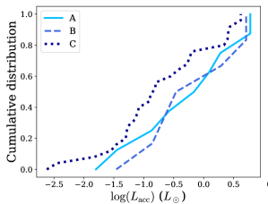
Figure 9: Cumulative distributions of accretion luminosities for clusters A (solid), B (dashed) and C (dotted line), as defined in Sewiło et al. (2019). Sources without $A_{\rm{V}}$ estimates are excluded.

4.2 A Possible Impact of Low Metallicity

Observations of star formation in external galaxies suggest that subsolar metallicity has a clear impact on the physical and chemical conditions in molecular clouds (e.g., Madden et al., 2013; Roman-Duval et al., 2014). In particular, a lower dust content in the low-metallicity environments reduces the shielding from ultraviolet radiation and translates to a decrease of molecular abundances due to photodissociation (“CO-dark gas”, e.g., Wolfire et al., 2010). The formation rate of molecules on the dust grains also decreases, which is the main reason for the reduction of H₂ abundances in the low-metallicity clouds (Glover & Clark, 2012).

The Large and Small Magellanic Clouds, with Z of $\sim$0.3-0.5 Z_⊙ (LMC; Russell & Dopita, 1992; Westerlund, 1997; Rolleston et al., 2002) and 0.2 Z_⊙ (SMC; Russell & Dopita, 1992), are routinely used as laboratories for studying star formation in low-metallicity environments. Observations show a decrease of molecular gas cooling in YSO envelopes, UV radiation penetrating deeper into the clouds, and an increase in average dust temperatures with respect to those in local star forming regions (e.g., van Loon et al., 2010b, a; Oliveira et al., 2019). However, the distances of 50.0$\pm$1.1 kpc (LMC, Pietrzyński et al. 2013) and 62.1$\pm$2.0 kpc (SMC, Graczyk et al. 2014) hinder characterisation of individual low-mass YSOs.

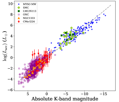
Figure 10: Accretion luminosity versus absolute $K$-band magnitude. Red stars show YSOs in CMa-$\ell$224, blue circles show MYSOs (Cooper et al., 2013), light-green “+” symbols show MYSOs from SMC (Ward et al., 2017), green crosses show MYSOs from LMC (Ward et al., 2016), violet open squares show YSOs in Orion (Manara et al., 2012), and orange triangles show low-mass YSOs in Perseus (Fiorellino et al., 2021). The dashed lines show linear fits separately to each of the datasets with the same colors. The grey line show a linear fit to all datapoints. All luminosities have been corrected for extinction.

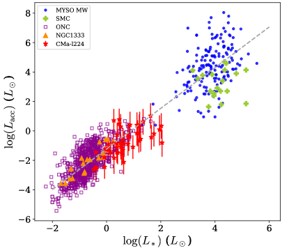
Figure 11: Accretion luminosity versus star luminosity. The symbols are the same as in Fig. 10. The dashed line show a linear fit to the data. All luminosities have been corrected for extinction.

The outer Galaxy also consists of star forming regions with the subsolar metallicities, and so offers the opportunity to study the impact of low metal content on star formation (Sodroski et al., 1997). The metallicity of CMa-$\ell$224 has not been measured, so here we adopt the O/H Galactocentric radial gradients obtained from the observations of HII regions accross the Milky Way. Depending on the adopted survey, the metallicity of CMa-$\ell$224 would be 0.55-0.58 Z_⊙ (Esteban & García-Rojas, 2018), 0.68 Z_⊙ (Fernández-Martín et al., 2017), or 0.67-0.73 Z_⊙ (Balser et al., 2011). The O/H and Fe/H gradients obtained using the observations of Cepheids suggest much higher metallicities of 1.11-1.17 Z_⊙ (Maciel & Andrievsky, 2019) or 1.13-1.27 Z_⊙ (Luck & Lambert, 2011), yet they are not representative for star forming regions. Therefore, we assume that the metallicity of CMa-$\ell$224 is intermediate between the metallicity of the LMC and the metallicity in the Solar neighborhood.

A possible effect of metallicity on YSO accretion has been investigated in the LMC and SMC based on the near-IR observations of massive YSOs (Ward et al., 2016, 2017), and optical observations with H$\alpha$ in YSOs with a wide range of masses (De Marchi et al., 2011, 2017; Biazzo et al., 2019). The Br$\gamma$ luminosities for Magellanic YSOs seem higher than those found in the Galactic high-mass YSOs from the RMS survey for the same absolute magnitudes (Cooper et al., 2013). Here, we extend the measurements toward lower-mass YSOs, which are located in CMa-$\ell$224 and more nearby star-forming regions (Figs. 10 and 11). We adopt the same empirical relations between the Br$\gamma$ luminosity and accretion luminosities for various samples (Alcalá et al., 2017); however, $L_{\mathrm{acc}}$ from Orion has been calculated using H$\alpha$ and two-color diagrams (Manara et al., 2012). The $K$-band magnitudes of YSOs from Orion are adopted from Robberto et al. (2010).

Figures 10 and 11 show the increase of $L_{\mathrm{acc}}$ with both the absolute $K$-band magnitude and $L_{*}$, with the YSOs from CMa-$\ell$224 located between the least massive YSOs in the NGC 1333 cluster in Perseus (Fiorellino et al., 2021) and in Orion (Manara et al., 2012), and the high-mass YSOs both in the Milky Way (Cooper et al., 2013) and the Magellanic Clouds (Ward et al., 2016, 2017). The Pearson coefficient of $|r|=0.96$ (30$\sigma$) is obtained for the absolute $K$-band magnitude vs. $L_{\mathrm{acc}}$ relation, reflecting a strong correlation (Fig. 10). Similarly, the Pearson coefficient of $|r|=0.93$ (30$\sigma$) characterises the $L_{*}$ vs $L_{\mathrm{acc}}$ relation.

Accretion luminosities in CMa-$\ell$224 are consistent with those in the Solar neighbourhood (e.g., Perseus, Orion) and do not show a clear enhancement of accretion luminosity expected in the low-metallicity environments (Ward et al., 2016, 2017). Most of the Br$\gamma$ emitters are however Class II sources, characterized by lower $L_{\mathrm{acc}}$ with respect to less evolved, Class I sources. The metallicity of CMa-$\ell$224 ($\sim$0.6-0.7 Z_⊙, Esteban & García-Rojas, 2018; Fernández-Martín et al., 2017; Balser et al., 2011) might be too similar to the Solar neighbourhood to exhibit a clear, measurable difference in accretion properties. Follow-up observations of additional clouds in the outer Galaxies, spanning a broad range of metallicities and sufficient number of sources, would be critical to draw robust conclusions about the impact of the lower metallicity on accretion rates in the Outer Galaxy.

5 Conclusions

We presented VLT/KMOS near-IR spectroscopy of YSOs in CMa-$\ell$224, illustrating the instrument capability to study low-mass star formation, and where applicable, to detect molecular outflows in the outer Galaxy. We summarise the findings as follows:

• The Br$\gamma$ line is detected in emission toward 47% and in absorption toward 13% of the sources. The H₂ 1-0 S(1) line is detected on-source in 33 sources, including 27 sources where the emission is extended. The CO bandhead at 2.3 $\mu$m is detected in emission in 5% of YSOs and in absorption in 60% of YSOs.

• The extent and velocity structures of H₂ emission suggest an origin of the emission in outflows and shocks. Follow-up observations are necessary, however, to estimate the extinction along the outflows.

• We find a gradual increase in accretion luminosities from Cluster C to A and B with median values of -0.89, -0.56, and -0.37 $\log{L_{\odot}}$, respectively. Cluster C might be the most evolved part of CMa-$\ell$224.

• Accretion luminosities do not show the impact of sub-Solar metallicity in the CMa-$\ell$224. It is likely due to insufficient difference in metallicity between the region and the Solar neighbourhood.

Large-scale galactic surveys, such as the Outer Galaxy High Resolution Survey (Colombo et al., 2021), are starting to provide a complete census of molecular clouds and star-forming filaments spanning a range of metallicities. IFU observations of YSOs in those regions, either with ground-based facilities or the James Webb Space Telescope, will be critical to confirm the impact of metallicity on low-mass star formation within our Galaxy.

Appendix A KMOS $K$-Band Continuum Maps

Figure A.1 shows the $K$-band continuum flux density maps for YSO candidates in CMa-$\ell$224 without stellar companions. Similar maps for the fields with the detection of two sources (the binary star candidates) are shown in Figure 2. Figure A.2 shows the integrated continuum maps for YSO candidates with the very weak $K$-band continuum.

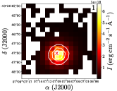
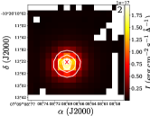
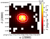
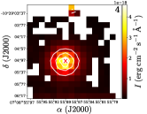
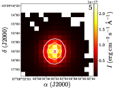
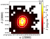
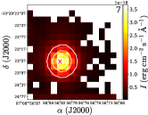
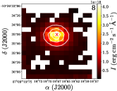
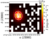
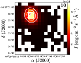
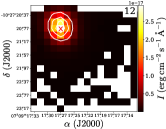
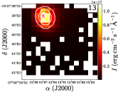
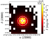
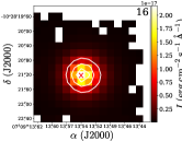
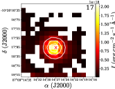
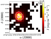
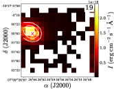
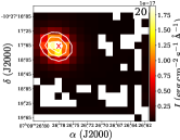
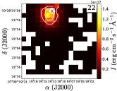
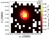
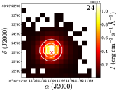
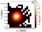
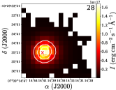
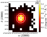
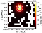
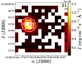
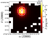
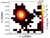
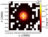
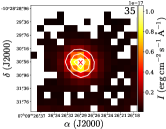
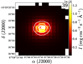
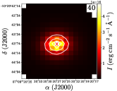
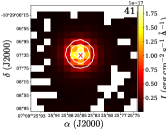
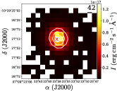
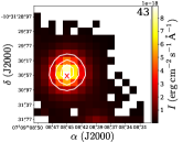
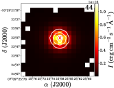
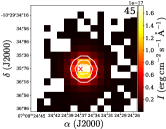
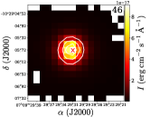
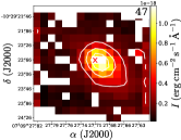
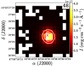
Figure A.1: KMOS $K$-band continuum maps for single YSO candidates. Source names are provided in the upper right corners (No. in Table 2). The contour levels are 0.25, 0.5, and 0.75$\times$ the $K$-band continuum peak. Only pixels with the continuum flux density above 3$\sigma$ are shown.

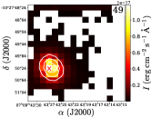
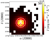
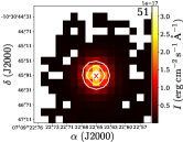
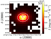
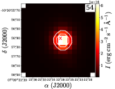
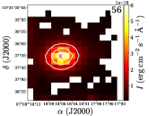
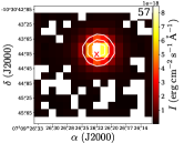
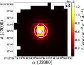
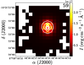
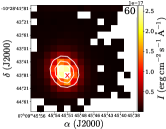
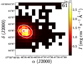
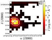
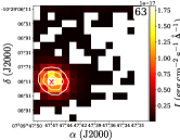
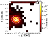
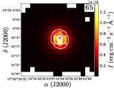
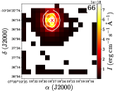
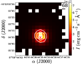
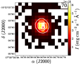
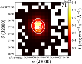
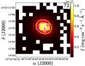
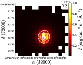
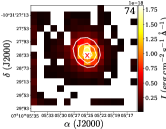
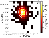
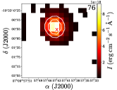
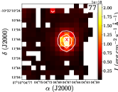
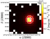
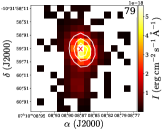
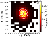
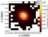
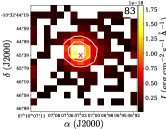
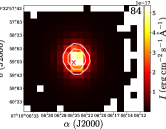
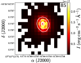
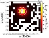
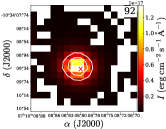
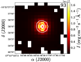
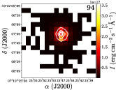
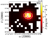
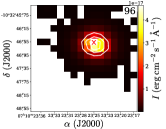
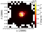
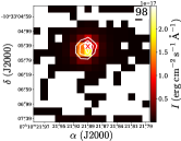
Figure A.1: Continued

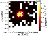
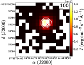
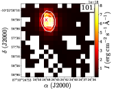
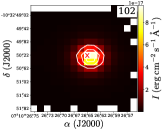
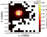
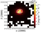
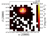
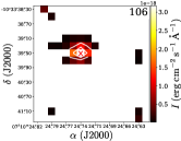
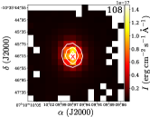
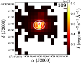
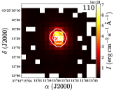
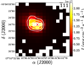
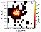
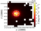
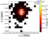
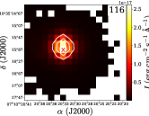
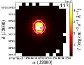
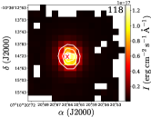
Figure A.1: Continued

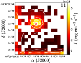
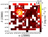
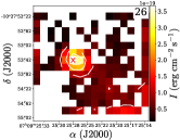
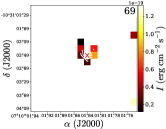
Figure A.2: Similar to Figure A.1, but for the faintest sources in the sample: No. 11, 14, 26, and 69 (see Table 2). The continuum was integrated over the entire $K$-band spectrum in every pixel to increase the signal-to-noise ratio.

Appendix B Spectra

Figures B.1-B.10 show the $K$-band spectra of all YSO candidates in CMa-$\ell$224 observed with KMOS. The spectra are presented in subgroups having similar characteristics – line detections and their profiles. In particular, Figure B.1 shows spectra of sources with the Br$\gamma$ line in emission, as represented by source No. 12 in Figure 3. Figure B.2 presents spectra of sources with the detections of both the Br$\gamma$ and H₂ at 2.12 $\mu$m lines in emission, but a lack of the CO bandhead emission. Figure B.3 shows spectra of two sources with the strong H₂ emission from outflows, but a lack of the Br$\gamma$ or CO bandhead lines. Figure B.4 shows spectra of three sources with the Br$\gamma$ and H₂ lines in emission, and the CO bandhead lines in absorption. Figure B.5 features spectra of presumably more evolved objects without the H₂ emission lines, but with the Br$\gamma$ line in emission and the CO bandhead lines in absorption. Figure B.6 shows spectra of sources with the H₂ emission and the CO bandhead absorption lines, but a lack of the Br$\gamma$ emission. Figure B.7 shows spectra of sources with the detection of Br$\gamma$ in absorption, and Figure B.8, the only five single sources with spectra characterised by the CO bandhead in emission. Figure B.9 shows spectra of sources with CO in absorption, but non-detections of the H₂ or Br$\gamma$ lines. Finally, Figure B.10 shows spectra of YSO candidates which do not show any signatures of accretion or ejection, and require follow-up observations to confirm their status.

Spectra of the individual components of the binary YSO candidates are presented in Figures B.11-B.12. While all spectra of single objects were extracted from the spectral cubes within the aperture of radius of 3 pixels, due to their proximity, for double stars different approach has been followed. For the most distant pairs (sources No. 21, 38, 38, 86, and 87) the same aperture radius was used. For sources No. 82, 91, and 112 we used the radius of 2 pixels. To maximise the collected signal, we used the radius of 1.5 pixels for pairs No. 52 and 55. Spectra of the barely resolved binary, source No. 89, were extracted using the 1 pixel radius. Their signal can be contaminated.

Table 4 provides an inventory of the key line detections in all sources, while Table 5 lists the measured H₂ line fluxes not corrected for extinction. We include only detections above 3$\sigma$.

Table 4: Detections.

No.	H2	Brγ	He I	Ca I	Mg I	Na I	Si I	K I	CO
2	E	N	N	A	A	A	N	N	N
47	E	N	N	N	N	N	N	N	N
87A	E	N	A	A	N	N	N	A	N
87B	E	N	A	A	A	A?	N	A	N
9	E	E	E	A	A	A	N	N	N
13	E	E	A	A?	N	N	N	A	N
15	E	E	A	A	A	A	N	A	N
26	E	E	?	A?	N	A	N	E	N
33	E	E	E	A	N	N	N	E	N
50	E	E	A	A	A	A	A?	A	N
54	E	E	N	A	?	N	N	A	N
60	E	E	E?	A	N	N	N	E?	N
83	E	E	A	A?	A?	N	?	A	N
111	E	E	E?	A	A	A	A?	E	N
112B	E?	E	A	?	N	N	N	A	N
114	E	E	E	?	N	A?	N	E	N
4	E	N	A?	A	A	A	N	A	A
7	E	N	A	A	A	A	A?	A	A
35	E	N	?	A	A	A	N	A	A
72	E	?	A?	A	A	A	A?	A	A
78	E	N	E	A	A	A	A	E	A
100	E	N	A	A	A	A	?	A	A
49	E	E	E	A	A	A	A?	E	A
73	E	E	E	A	A	A	E	E	A?
91B	E	E	N	A	A?	A	A	?	A
109	E	E	A	A	A	A	N	A	A
16	N	E	N	A	A	A	A?	N	N
24	N	E	N	A	A	A	N	A	N
28	N	E	N	A	A	A	A	A	N
31	N	E	?	A	N	N	N	A?	N
36A	N	E	N	A	A	A	A	N	N
41	N	E	N	A	A	N	N	A	N
56	N	E	A	A	A	A	N	A	N
79	N	E	A	A	N	A	N	A	N
81	N	E	A	A	A	A?	N	A?	N
85	N	E	A	A	A	A	N	A	N
93	N	E	E	A	N	A	E?	E	N
102	N	E	N	A	A	A	N	N	N
118	N	E	E	A	A	A	A?	E	N
3	N	E	N	A	A	A	A?	A	A
6	N	E	N	A	A	A	A?	A	A
10	N	E	E	A	A	A	N	E?	A?
12	N	E	E?	A	A	A	A?	N	A
18	N	E	E	A	A	A	A	E	A
20	N	E	A?	A	A	A	A	N	A
22	N	E	E	A	A	A	A?	E	A
23	N	E	E	A	A	A	A?	E?	A
30	N	E?	E?	A	A	A	A?	N	A
32	N	E	N	A	A	A	A	N	A
34	N	E	E	A	A	A	A	E?	A
38A	N	E	A	A	A	A	A?	E	A
38B	N	E	A	A	A	A?	A?	E	A
48	N	E	E?	A	A	A	A	N	A
52A	N	E	A	A	A	A	A	A	A
52B	N	E	A	A	A	A	A	A	A
55A	N	E	E?	A	A	A	A	E?	A
57	N	E	A?	A	A	A	N	A?	A
80	N	E	A	A	A	A	A	A	A
89A	N	E?	A	A	A	A	A?	A	A
97	N	E	A	A	A	A	A?	A?	A
98	N	E	A	A	A	A	A?	A	A
99	N	E	E	A	?	A	E?	E?	A
5	N	A	N	A	A	A	A	N	A
40	N	A	N	A	A	A	A	N	A
43	N	A	N	A	A	A	A	A?	A
53	N	A	N	A	A	N	N	A	N
61	N	A	E?	A	A	A	A	E	A
63	N	A	E?	A	A	A	A	E	A
65	N	A	N	A	A	A	A	N	A
71	N	A	A	A	A	A?	?	A	A
75	N	A	A	A?	A	N	A?	A	N
84	N	A	N	A	A	A	A	E?	A
91A	E	A	A?	A	A	A	A	E?	A
92	N	A	A	A	A	N	N	A	N
94	N	A	A	A	A	A	A?	A?	A
96	N	A	A	A	A	A	A?	A	A
104	N	A	A?	A	A	A	A	E?	A
116	N	A	A	A	A	A	A	E	A?
19	E	E	E	N	N	N	N	E	E
39	E?	E	N	A	A	A	N	N	E
46	E	E	N	A	A	N	N	N	E
64	E	E	E	A	A?	N	N	E	E
77	E	E	E	A?	A?	A?	E?	E	E
112A	E?	E	A	?	N	N	N	A	E
25	N	N	N	A	A	A	A	A	A
29	N	N	A?	A	A	A	A	A	A
42	N	N	E?	A	A	A	N	E?	A
44	N	N	N	A	A	A	A?	A?	A
45	N	N	N	A	A	A	N	N	A
51	N	N	N	A	A	A	A	N	A
55B	N	N	E	A	A	A	A?	E?	A
58	N	N	E?	A	A	A	A?	N	A
59	N	N	?	A	A	A	A?	N	A
66	N	N	A	A	A	A	A	N	A
68	N	N	N	A	A	A	A	E?	A
69	N	N	E?	A	A?	A?	N	A	A?
70	N	N	A	A	A	A	A?	A	A
74	N	N	E?	A	A	A	?	A	A
82A	N	N	A	A	A	A	A?	A	A
82B	N	N	A	A	A	A	A?	A	A
86A	N	N	N	A	A	A	A?	A	A
86B	N	N	?	A	A?	A	A?	A?	A
89B	N	N	?	A	A	A	A?	A	A
95	N	N	E	A	A	A	N	E	A?
101	N	N	E?	A	N	A	E?	E	A
103	N	N	A?	A	A	A	A?	E	A
105	N	N	E	A	A	A	A	E	A
108	N	N	E	A	A	A	A	E	A
110	N	N	E	A	A	A	A?	E	A
113	N	N	A	A	A	A	A	A	A
115	N	N	A	A	A	A	A	A	A
117	N	N	E	A	A	A	A	E	A
1	N	N	?	A	A	A	A	E?	N
8	N	N	N	A	A?	A?	N	A	N
11	N	N	E	A	A	N	N	A	N
14	N	N	E	A?	A	N	E?	E	N
17	N	N	A	A	A	A	N	A	N
21A	N	N	A?	?	N	N	N	A	N
21B	N	N	A?	?	A	N	N	A	N
62	N	N	E	A	A	A	N	E	N
76	N	N	?	N	A?	N	?	A?	N
90	N	N	A	A?	A?	N	N	A	N
106	N	N	A	A	N	A?	N	A	N

Note. — E indicates emission line, A - absorption, N - no detection, ? - possible detection.

=-3cm

Table 5: H₂ Emission Line Fluxes.

No.	1-0 S(0)	1-0 S(1)	1-0 S(2)	1-0 S(3)	2-1 S(1)	2-1 S(2)	2-1 S(3)	No.	1-0 Q(1)	1-0 Q(2)	1-0 Q(3)	1-0 Q(4)	1-0 Q(5)	1-0 Q(6)
	($\rm 10^{-16}~{}erg~{}s^{-1}cm^{-2}$)								($\rm 10^{-16}~{}erg~{}s^{-1}cm^{-2}$)
2	5.35 $\pm$ 0.33	25.61 $\pm$ 0.58	10.18 $\pm$ 0.38	36.90 $\pm$ 3.39	$\cdots$	$\cdots$	2.24 $\pm$ 0.87		25.77 $\pm$ 1.54	5.97 $\pm$ 1.86	22.60 $\pm$ 1.10	$\cdots$	16.72 $\pm$ 1.14	5.40 $\pm$ 1.37
4*	1.55 $\pm$ 0.16	3.36 $\pm$ 0.20	0.85 $\pm$ 0.11	6.27 $\pm$ 1.19	0.97 $\pm$ 0.26	$\cdots$	$\cdots$		5.38 $\pm$ 0.84	$\cdots$	4.99 $\pm$ 0.65	$\cdots$	2.98 $\pm$ 0.56	$\cdots$
7*	$\cdots$	0.87 $\pm$ 0.15	$\cdots$	$\cdots$	$\cdots$	$\cdots$	$\cdots$		$\cdots$	$\cdots$	$\cdots$	$\cdots$	2.57 $\pm$ 0.76	$\cdots$
9	$\cdots$	1.62 $\pm$ 0.12	$\cdots$	1.83 $\pm$ 0.51	$\cdots$	$\cdots$	$\cdots$		$\cdots$	$\cdots$	$\cdots$	$\cdots$	$\cdots$	$\cdots$
13	$\cdots$	2.33 $\pm$ 0.56	$\cdots$	3.26 $\pm$ 0.93	$\cdots$	$\cdots$	$\cdots$		$\cdots$	$\cdots$	$\cdots$	$\cdots$	$\cdots$	$\cdots$
15	$\cdots$	4.42 $\pm$ 0.27	$\cdots$	7.84 $\pm$ 2.26	1.91 $\pm$ 0.31	$\cdots$	$\cdots$		5.70 $\pm$ 1.22	$\cdots$	6.59 $\pm$ 1.45	$\cdots$	4.21 $\pm$ 0.92	$\cdots$
19	1.52 $\pm$ 0.25	5.30 $\pm$ 0.22	2.62 $\pm$ 0.24	5.14 $\pm$ 0.84	1.21 $\pm$ 0.31	$\cdots$	$\cdots$		6.21 $\pm$ 0.83	$\cdots$	6.71 $\pm$ 0.90	$\cdots$	3.62 $\pm$ 1.02	2.24 $\pm$ 0.67
26	$\cdots$	1.51 $\pm$ 0.20	0.86 $\pm$ 0.20	$\cdots$	$\cdots$	$\cdots$	$\cdots$		$\cdots$	$\cdots$	$\cdots$	$\cdots$	$\cdots$	$\cdots$
33	0.94 $\pm$ 0.30	2.17 $\pm$ 0.16	0.83 $\pm$ 0.15	5.43 $\pm$ 1.39	$\cdots$	$\cdots$	$\cdots$		3.53 $\pm$ 0.75	$\cdots$	3.30 $\pm$ 1.00	$\cdots$	$\cdots$	$\cdots$
35	$\cdots$	3.24 $\pm$ 0.31	$\cdots$	$\cdots$	$\cdots$	$\cdots$	$\cdots$		$\cdots$	$\cdots$	$\cdots$	$\cdots$	$\cdots$	$\cdots$
39	$\cdots$	12.53 $\pm$ 1.57	$\cdots$	$\cdots$	$\cdots$	$\cdots$	$\cdots$		$\cdots$	$\cdots$	22.78 $\pm$ 2.78	$\cdots$	$\cdots$	$\cdots$
46	$\cdots$	12.92 $\pm$ 0.60	6.16 $\pm$ 0.81	$\cdots$	$\cdots$	$\cdots$	$\cdots$		$\cdots$	$\cdots$	$\cdots$	$\cdots$	$\cdots$	$\cdots$
47	17.48 $\pm$ 0.52	69.91 $\pm$ 1.05	22.15 $\pm$ 0.51	76.05 $\pm$ 2.38	7.43 $\pm$ 0.40	3.09 $\pm$ 0.36	6.19 $\pm$ 0.34		85.63 $\pm$ 2.80	24.76 $\pm$ 0.95	76.93 $\pm$ 2.74	20.75 $\pm$ 3.33	26.15 $\pm$ 1.24	10.96 $\pm$ 2.36
49	$\cdots$	4.65 $\pm$ 0.34	3.14 $\pm$ 0.47	$\cdots$	$\cdots$	$\cdots$	3.30 $\pm$ 0.59		6.04 $\pm$ 0.53	$\cdots$	4.87 $\pm$ 0.53	$\cdots$	$\cdots$	$\cdots$
50	$\cdots$	1.47 $\pm$ 0.18	0.49 $\pm$ 0.17	4.37 $\pm$ 1.22	$\cdots$	$\cdots$	$\cdots$		$\cdots$	$\cdots$	2.09 $\pm$ 0.56	$\cdots$	4.97 $\pm$ 1.02	$\cdots$
54*	23.05 $\pm$ 6.16	75.32 $\pm$ 14.15	$\cdots$	123.66 $\pm$ 27.71	$\cdots$	$\cdots$	$\cdots$		$\cdots$	$\cdots$	$\cdots$	$\cdots$	$\cdots$	$\cdots$
60	14.58 $\pm$ 0.69	60.13 $\pm$ 0.47	23.57 $\pm$ 0.71	99.90 $\pm$ 13.36	7.30 $\pm$ 0.79	2.74 $\pm$ 0.36	5.84 $\pm$ 1.29		65.22 $\pm$ 3.30	12.80 $\pm$ 1.80	58.16 $\pm$ 2.53	39.66 $\pm$ 9.77	24.78 $\pm$ 5.70	13.01 $\pm$ 4.73
64	3.11 $\pm$ 0.42	9.67 $\pm$ 0.45	4.86 $\pm$ 0.23	$\cdots$	$\cdots$	0.79 $\pm$ 0.25	2.45 $\pm$ 0.77		10.93 $\pm$ 1.08	4.87 $\pm$ 1.14	11.93 $\pm$ 0.62	$\cdots$	$\cdots$	3.51 $\pm$ 1.05
73	$\cdots$	1.64 $\pm$ 0.32	2.45 $\pm$ 0.26	$\cdots$	$\cdots$	0.69 $\pm$ 0.13	$\cdots$		2.78 $\pm$ 0.58	$\cdots$	2.49 $\pm$ 0.33	$\cdots$	2.37 $\pm$ 0.53	$\cdots$
77	$\cdots$	1.37 $\pm$ 0.14	2.43 $\pm$ 0.26	$\cdots$	0.40 $\pm$ 0.14	$\cdots$	$\cdots$		1.64 $\pm$ 0.46	$\cdots$	$\cdots$	$\cdots$	$\cdots$	$\cdots$
83	$\cdots$	2.88 $\pm$ 0.26	$\cdots$	3.25 $\pm$ 1.01	$\cdots$	$\cdots$	$\cdots$		$\cdots$	$\cdots$	$\cdots$	$\cdots$	$\cdots$	$\cdots$
87A	0.49 $\pm$ 0.17	2.11 $\pm$ 0.19	$\cdots$	$\cdots$	$\cdots$	$\cdots$	$\cdots$		1.52 $\pm$ 0.52	$\cdots$	1.17 $\pm$ 0.33	$\cdots$	$\cdots$	$\cdots$
87B	$\cdots$	0.66 $\pm$ 0.08	$\cdots$	$\cdots$	$\cdots$	$\cdots$	$\cdots$		0.40 $\pm$ 0.17	$\cdots$	$\cdots$	$\cdots$	$\cdots$	$\cdots$
91A*	$\cdots$	11.73 $\pm$ 1.70	$\cdots$	17.49 $\pm$ 4.68	$\cdots$	5.43 $\pm$ 1.05	$\cdots$		20.27 $\pm$ 6.68	$\cdots$	17.11 $\pm$ 4.79	$\cdots$	$\cdots$	$\cdots$
91B*	1.21 $\pm$ 0.32	4.84 $\pm$ 0.26	1.93 $\pm$ 0.32	4.14 $\pm$ 0.56	$\cdots$	$\cdots$	0.79 $\pm$ 0.23		5.87 $\pm$ 0.50	$\cdots$	4.77 $\pm$ 0.25	$\cdots$	$\cdots$	$\cdots$
100*	2.56 $\pm$ 0.28	10.07 $\pm$ 0.25	3.77 $\pm$ 0.54	6.33 $\pm$ 0.92	1.40 $\pm$ 0.25	$\cdots$	$\cdots$		8.61 $\pm$ 0.48	2.63 $\pm$ 0.67	6.22 $\pm$ 0.38	$\cdots$	$\cdots$	$\cdots$
109	2.12 $\pm$ 0.18	9.18 $\pm$ 0.46	2.61 $\pm$ 0.27	7.89 $\pm$ 1.44	0.80 $\pm$ 0.14	$\cdots$	$\cdots$		9.26 $\pm$ 0.42	2.91 $\pm$ 0.56	6.85 $\pm$ 0.66	$\cdots$	$\cdots$	$\cdots$
111	$\cdots$	3.93 $\pm$ 0.90	2.14 $\pm$ 0.49	$\cdots$	$\cdots$	$\cdots$	$\cdots$		$\cdots$	$\cdots$	$\cdots$	$\cdots$	$\cdots$	$\cdots$
112A	0.27 $\pm$ 0.03	0.79 $\pm$ 0.16	$\cdots$	$\cdots$	$\cdots$	$\cdots$	$\cdots$		$\cdots$	$\cdots$	1.73 $\pm$ 0.34	$\cdots$	$\cdots$	$\cdots$
112B	$\cdots$	0.58 $\pm$ 0.15	0.25 $\pm$ 0.09	$\cdots$	$\cdots$	$\cdots$	$\cdots$		$\cdots$	$\cdots$	$\cdots$	$\cdots$	$\cdots$	$\cdots$
114	2.64 $\pm$ 0.31	10.46 $\pm$ 0.65	4.93 $\pm$ 0.19	6.72 $\pm$ 1.08	0.83 $\pm$ 0.25	1.69 $\pm$ 0.40	2.97 $\pm$ 0.69		12.57 $\pm$ 1.00	$\cdots$	9.87 $\pm$ 0.79	$\cdots$	$\cdots$	$\cdots$

Note. — H₂ line fluxes have not been corrected for extinction. Reported are only fluxes with detection significance above 3$\sigma$. Targets with asterisk do not have estimated extinction from SED models.

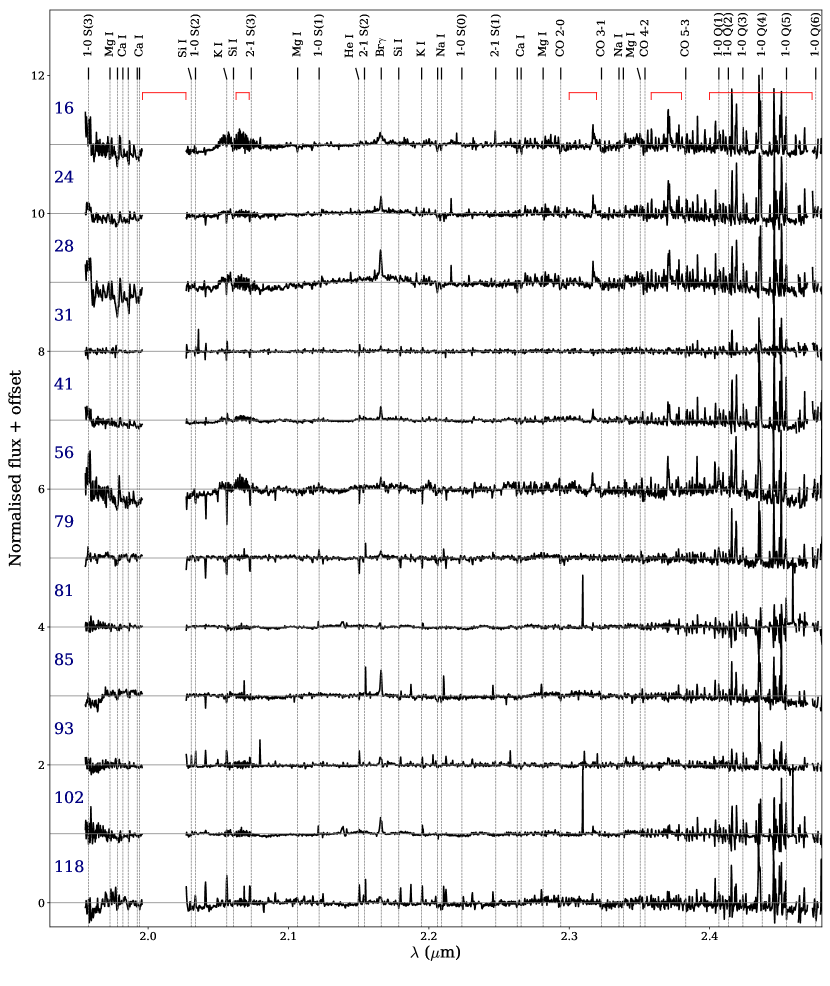
Figure B.1: $K$-band spectra of YSO candidates in the CMa-$\ell$224 star forming region, which show the H Br$\gamma$ line in emission. All spectra are continuum subtracted and normalised to the peak flux density in the range from 1.97 to 2.47 $\mu$m. Red horizontal lines show spectral ranges most affected by telluric lines; the range at 2.0 $\mu$m has been removed for clarity.

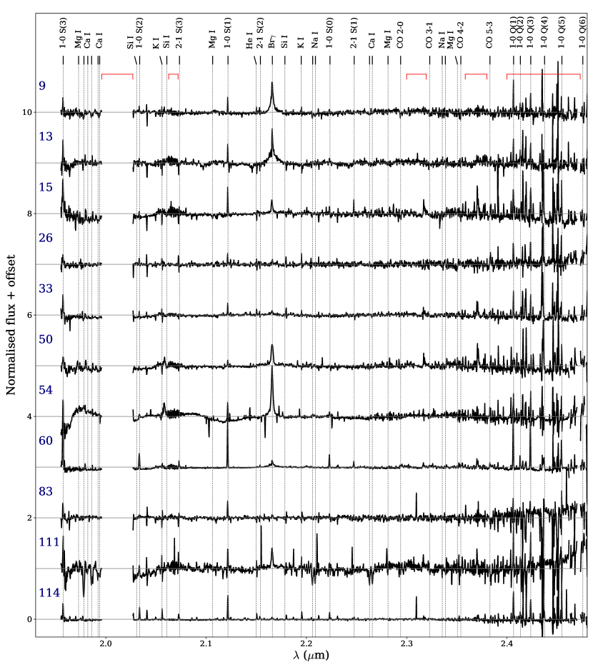
Figure B.2: Spectra with Br$\gamma$ and H₂ emission lines.

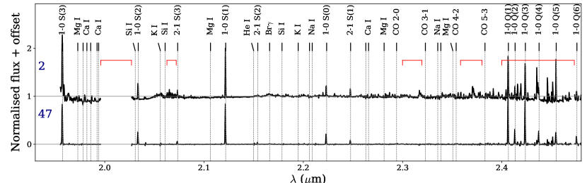
Figure B.3: Spectra with only H₂ emission lines.

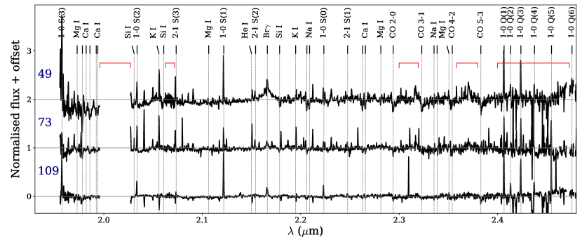
Figure B.4: Spectra with Br$\gamma$ and H₂ emission lines, and CO bandhead in absorption.

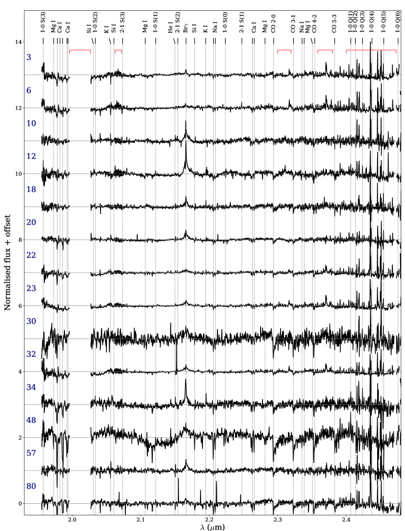
Figure B.5: Spectra with Br$\gamma$ emission line and CO bandhead in absorption.

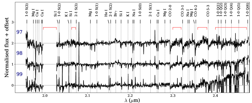
Figure B.5: Continuation.

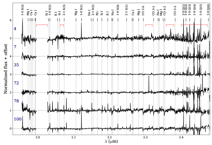
Figure B.6: Spectra with H₂ emission lines and CO bandhead in absorption.

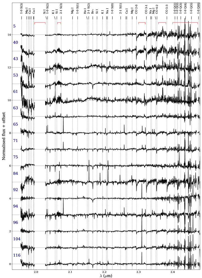
Figure B.7: Spectra with Br$\gamma$ absorption line.

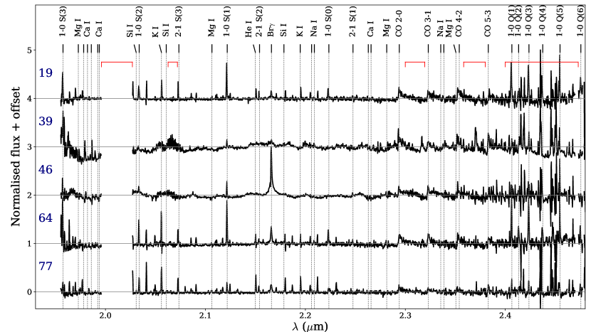
Figure B.8: Spectra with CO bandhead in emission.

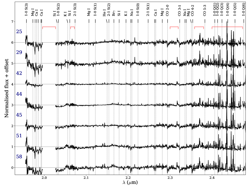
Figure B.9: Spectra with CO bandhead in absorption.

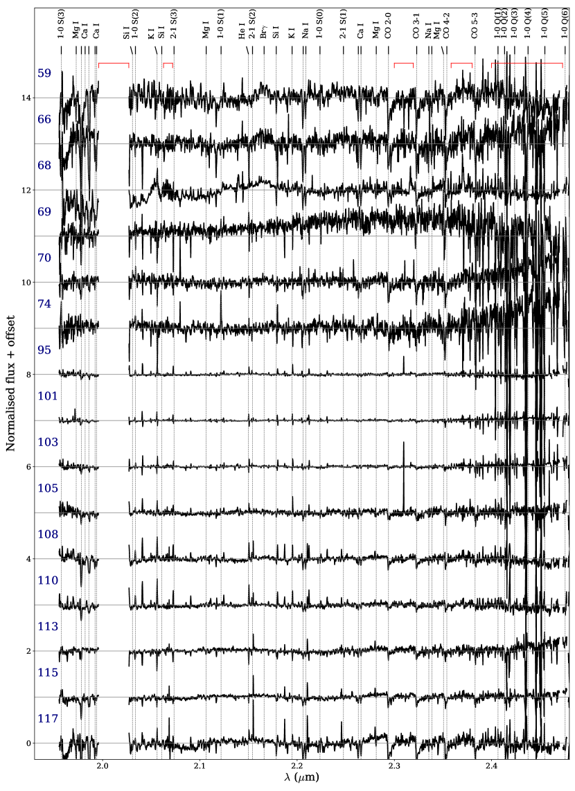
Figure B.9: Continuation.

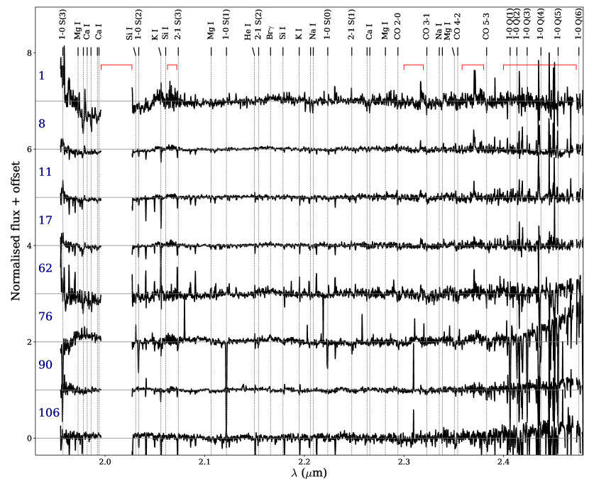
Figure B.10: Spectra with no emission lines and no CO or Br$\gamma$ absorption lines.

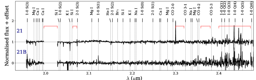
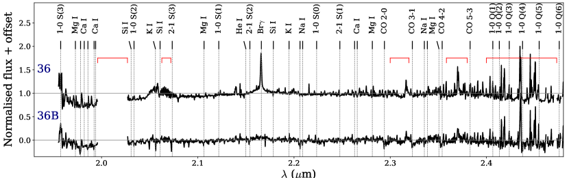
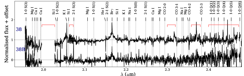
Figure B.11: Spectra from three pairs of double sources.

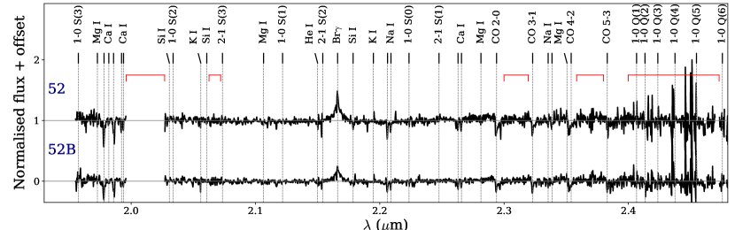
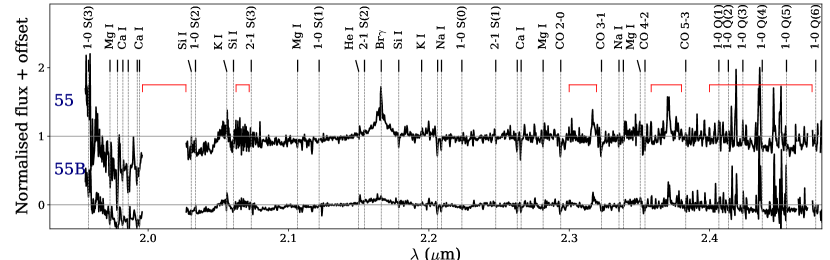
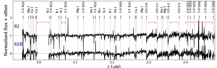
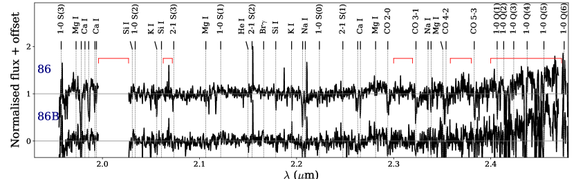
Figure B.12: Spectra from double sources - continuation.

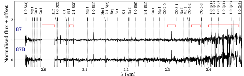
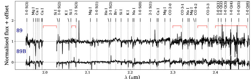
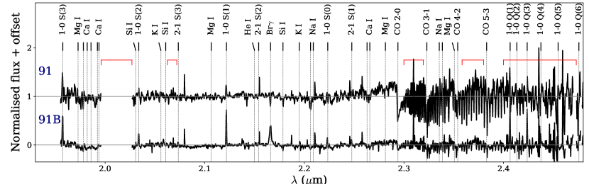
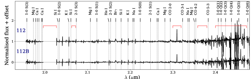
Figure B.12: Continuation.

Appendix C Line Emission Maps

Figures C.1–C.5 show the emission maps of the most commonly detected H₂ lines in the $K$-band range. Figure C.6 shows the spatial extent of several transitions of H₂ toward source No. 47, which has the most molecular-rich spectrum at $K$-band. Source No. 47 has the K-band magnitude of 15.2 based on our KMOS observations, thus it is one of the faintest sources in the sample. Sewiło et al. (2019) classified it as a Class I YSO. The young evolutionary stage of the source is confirmed by strong bipolar outflows. This source is an interesting case for detailed follow-up studies.

Figure C.7 shows the hydrogen Br$\gamma$ 2.17 $\mu$m emission maps. Figures C.8, C.9, C.10, and C.11 show the emission maps for several CO bandhead transitions – CO 2-0, 3-1, 4-2, and CO 5-3, respectively.

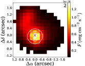
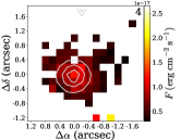
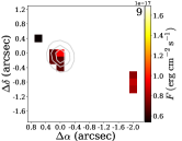
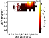
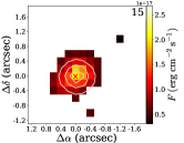
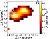
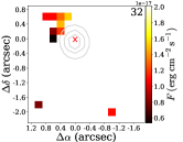
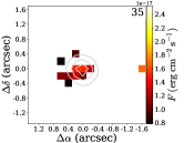
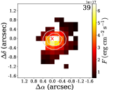
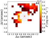
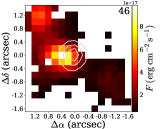
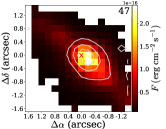
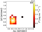
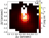
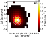
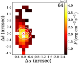
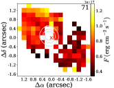
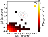
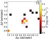
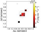
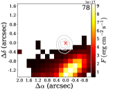
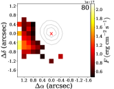
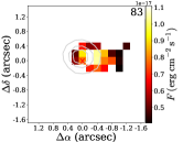
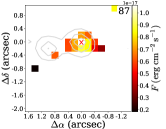
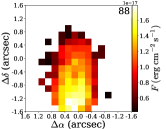
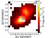
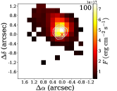
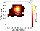
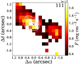
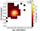
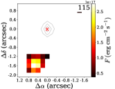
Figure C.1: Integrated maps of the H₂ 1-0 S(1) line at 2.1218 $\mu$m for a subsample of sources where the extended H₂ emission is detected (see Table 2). Colors correspond to the line fluxes at each pixel (detections above 3$\sigma$) and white contours correspond to the continuum emission in $K$-band (see also Appendix A). Source names are provided in the upper right corners (No. in Table 2). Note that source No. 88 (G224.4514$-$00.7054) has a non-detection of the continuum emission at 2.1218 $\mu$m.

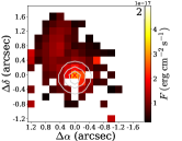
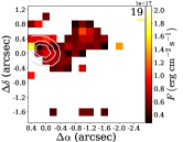
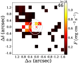
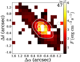
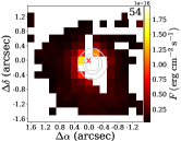
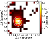
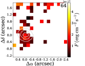
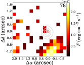
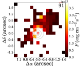
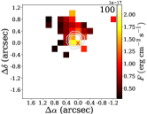
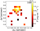
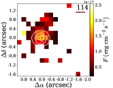
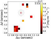
Figure C.2: Similar to Figure C.1, but for the H₂ 1-0 S(0) line at 2.2235 $\mu$m. Only emission above 2$\sigma$ is shown.

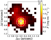
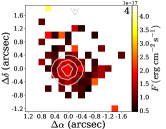
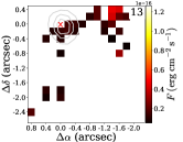
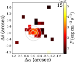
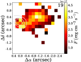
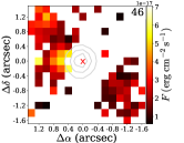
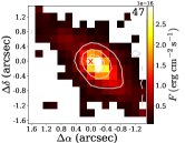
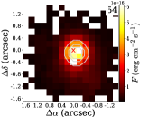
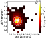
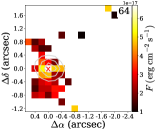
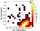
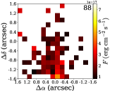
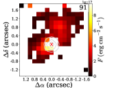
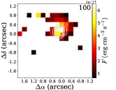
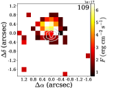
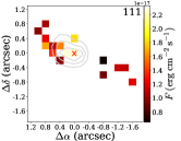
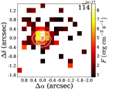
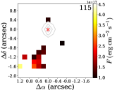
Figure C.3: Similar to Figure C.1, but for the H₂ 1-0 Q(1) line at 2.4066 $\mu$m. Only emission above 2$\sigma$ is shown.

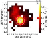
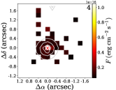
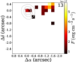
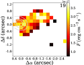
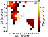
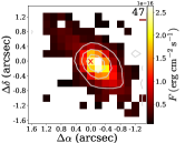
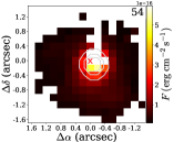
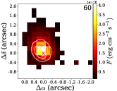
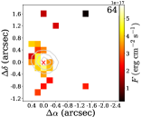
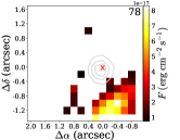
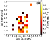
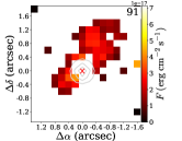
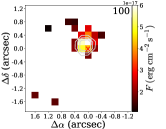
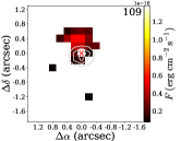
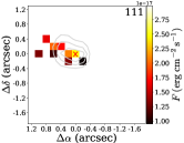
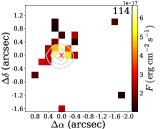
Figure C.4: Similar to Figure C.1, but for the H₂ 1-0 Q(3) line at 2.4237 $\mu$m. Only emission above 2$\sigma$ is shown.

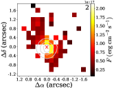
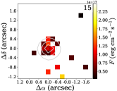
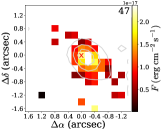
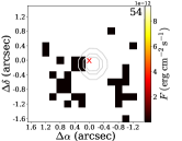
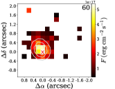
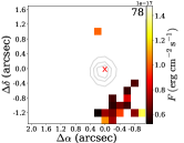
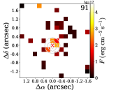
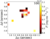
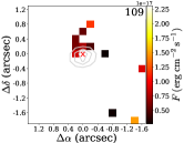
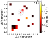
Figure C.5: Similar to Figure C.1, but for the H₂ 2-1 S(1) line at 2.2477 $\mu$m. Only emission above 2$\sigma$ is shown.

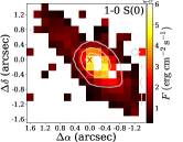
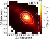
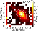
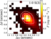
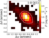
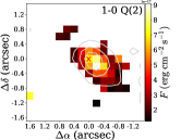
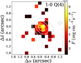
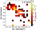
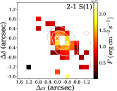
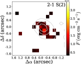
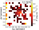
Figure C.6: Maps in several H₂ lines in source No. 47, which shows detections of the highest-excited H₂ lines in the entire sample (see Table 2).

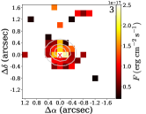
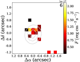
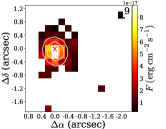
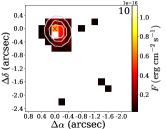
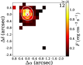
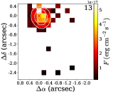
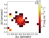
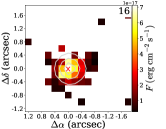
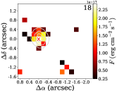
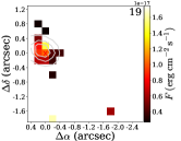
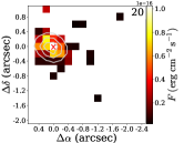
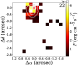
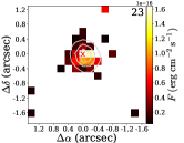
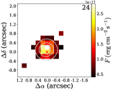
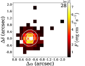
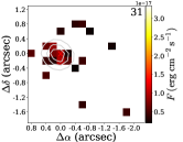
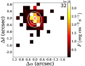
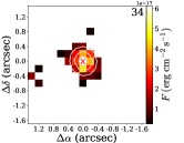
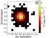
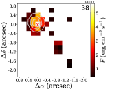
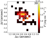
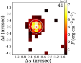
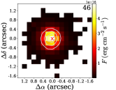
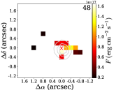
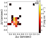
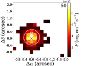
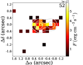
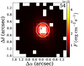
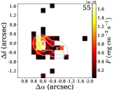
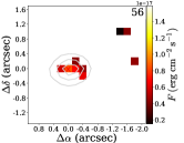
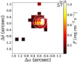
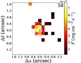
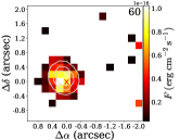
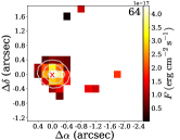
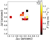
Figure C.7: Integrated maps for the H Br$\gamma$ line at 2.1661 $\mu$m. Colors correspond to the line fluxes at each pixel (detections above 2$\sigma$) and white contours show the continuum emission in $K$-band (see also Appendix A).

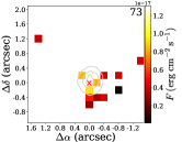
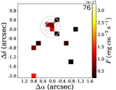
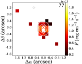
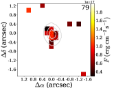
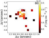
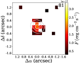
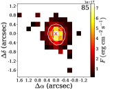
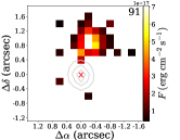
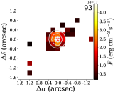
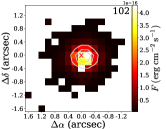
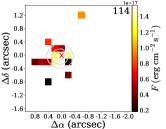
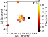
Figure C.7: Continued

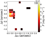
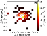
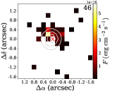
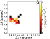
Figure C.8: Integrated maps of the CO $\nu$ = 2-0 line at 2.29 $\mu$m. Colors correspond to the line fluxes at each pixel (detections above 2$\sigma$) and white contours show the continuum emission in K-band (see also Appendix A).

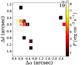
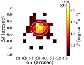
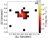
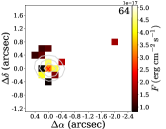
Figure C.9: Similar to Figure C.8, but the maps show the CO $\nu$ = 3-1 line at 2.32 $\mu$m.

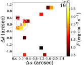
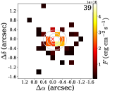
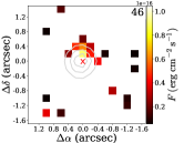
Figure C.10: Similar to Figure C.8, but the maps show the CO $\nu$ = 4-2 line at 2.35 $\mu$m.

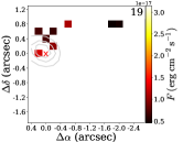
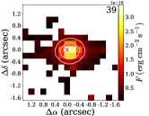
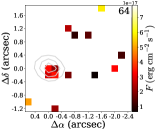
Figure C.11: Similar to Figure C.8, but the maps show the CO $\nu$ = 5-3 line at 2.38 $\mu$m.

Appendix D Extinction within stellar envelopes

The extinction values from SED modelling incorporate only the interstellar extinction to the source. Some of our stars were identified to be embedded in the envelope. Thus, to complete the estimations of extinction, we investigate the level of extinction due to the envelope. We consider only the targets, for which best-fit SED models included the envelope component (Sewiło et al., 2019). For simplicity, we assume that the spherical envelope can be well described by the power-law density profile (Robitaille, 2017b, Eq. 3):

$$\rho(r)=\rho_{0}\cdot(r/R_{0})^{\gamma}$$ (D1)

where $\rho_{0}$ is a volume mass density at the radius $R_{0}$ and $\gamma$ represents the slope of the relation. We do not include outflow cavities, which were considered in the original models.

To calculate column densities, we integrate the density profile along the line of sight, between the inner and outer radii of the envelope. We assume the mean molecular weight of 2.8 and the gas-to-dust ratio of 100. For calculations, we adopt parameter values from SED modelling of Sewiło et al. (2019) and set the outer radius to be at 5000 au (the maximum value considered in models of Robitaille 2017b). In cases where the inner radius was not available, we assume a value of 50 au. For target No. 47 we also assume the $R_{0}=100$ au, which is within the parameter range adopted in the SED modelling (Robitaille, 2017b). Some of our sources were originally fitted by a broken power-law density profile (Robitaille, 2017b, Eq. 4) and therefore they lack the value of $\gamma$. We assume a slope of -1/2 for $r<R_{0}$ and -3/2 for $r>R_{0}$, following the description in Sec. 3.2.3 of Robitaille (2017b).

We estimate the visual extinction due to the envelope of YSOs based on derived column densities. We follow the formula from Predehl & Schmitt (1995):

$$A_{\rm V}=1.086\cdot N\cdot\pi a_{g}^{2}\cdot Q_{\rm ext}$$ (D2)

where $N$ is a column density in 10²¹ cm^-2, $a_{g}$ is a radius of a spherical grain in 0.1 $\mu$m, and $Q_{\rm ext}$ is an extinction efficiency. We adopted $a_{g}$ = 0.1 $\mu$m and $Q_{\rm ext}$ = 0.5. The resulting estimates are shown in Fig. D.1 as a function of a total $A_{\rm V}$ obtained from the SED models. $A_{\rm{V,env}}$ is higher for most Class I than for Class II sources, indicating that envelope is being dissipated with time, in line with evolutionary predictions. The only outlier, Class II star No. 65, is characterised by high $\rho_{0}=1.8\times 10^{-18}$ g cm^-3, which leads to the very high value of the envelope extinction. This source is very bright, has relatively low $A_{\rm V}$, and has no emission lines, which are signposts of ongoing accretion or ejection. Clear detection of CO bandhead in absorption suggests that this target might be a foreground contamination, possibly a red giant.

Table 6: Interstellar and Envelope Extinction Values from SED Modeling.

No.					$A_{\rm{V,interst}}$	$A_{\rm{V,env}}$
1					8.04	$\cdots$
2					9.0	12.99
3					11.9	$\cdots$
5					34.9	3.98
6					23.4	$\cdots$
8					25.3	$\cdots$
9					30.8	$\cdots$
10					27.6	$\cdots$
12					31.0	$\cdots$
13					15.4	$\cdots$
15					40.0	$\cdots$
16					21.3	$\cdots$
19					33.9	$\cdots$
20					12.2	$\cdots$
24					27.0	$\cdots$
26					25.9	$\cdots$
28					9.92	$\cdots$
30					2.84	$\cdots$
32					6.84	$\cdots$
33					21.7	$\cdots$
35					20.0	2.06
39					10.2	$\cdots$
40					28.6	$\cdots$
42					26.2	$\cdots$
43					2.29	$\cdots$
45					19.3	$\cdots$
46					14.0	$\cdots$
47					33.3	12.65
48					3.03	$\cdots$
49					32.0	$\cdots$
50					15.7	$\cdots$
53					22.4	$\cdots$
55A					3.37	$\cdots$
55B					3.37	$\cdots$
56					22.0	$\cdots$
58					5.03	$\cdots$
59					2.9	$\cdots$
60					18.2	22.21
61					8.51	$\cdots$
62					17.3	$\cdots$
63					22.6	$\cdots$
64					7.15	28.74
65					3.84	109.96
68					7.19	$\cdots$
70					10.6	$\cdots$
71					27.8	$\cdots$
73					26.2	$\cdots$
75					23.1	$\cdots$
76					24.2	$\cdots$
77					40.0	0.00
79					15.1	$\cdots$
81					25.7	$\cdots$
82A					11.8	0.01
82B					11.8	0.01
83					12.8	41.15
84					17.3	3.13
86A					6.14	$\cdots$
86B					6.14	$\cdots$
87A					30.3	$\cdots$
87B					30.3	$\cdots$
88					0.0	0.23
92					9.37	$\cdots$
93					28.5	$\cdots$
94					8.96	$\cdots$
95					4.49	$\cdots$
96					19.1	0.04
97					13.9	$\cdots$
98					7.47	$\cdots$
102					15.4	$\cdots$
104					7.78	$\cdots$
105					28.1	$\cdots$
108					7.74	$\cdots$
109					15.0	29.33
110					16.9	$\cdots$
111					17.0	$\cdots$
112A					25.1	$\cdots$
112B					25.1	$\cdots$
113					21.7	$\cdots$
114					39.4	$\cdots$
115					9.23	15.27
116					2.43	$\cdots$
117					5.11	$\cdots$
118					12.7	$\cdots$

Note. — All values are given in magnitudes. $A_{\rm V,interst}$ is the value adopted from Sewiło et al. (2019) based on the SED modeling; we assume an uncertainty of 10 mag of their measurements (see text for details). The $A_{\rm V,env}$ is the extinction within the envelope estimated based on the results of the SED modeling.

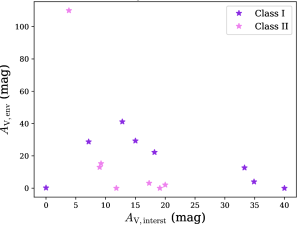
Figure D.1: Comparison between the total visual extinction $A_{\rm{V,total}}$ (Sewiło et al., 2019) and the extinction within the envelope $A_{\rm{V,env}}$. The latter was estimated assuming spherical envelope and a power-law density profile. See the text for details.

References

- Agra-Amboage et al. (2014) Agra-Amboage, V., Cabrit, S., Dougados, C., et al. 2014, A&A, 564, A11, doi: 10.1051/0004-6361/201220488
- Alcalá et al. (2014) Alcalá, J. M., Natta, A., Manara, C. F., et al. 2014, A&A, 561, A2, doi: 10.1051/0004-6361/201322254
- Alcalá et al. (2017) Alcalá, J. M., Manara, C. F., Natta, A., et al. 2017, A&A, 600, A20, doi: 10.1051/0004-6361/201629929
- André (2017) André, P. 2017, Comptes Rendus Geoscience, 349, 187, doi: 10.1016/j.crte.2017.07.002
- Ansdell et al. (2017) Ansdell, M., Williams, J. P., Manara, C. F., et al. 2017, AJ, 153, 240, doi: 10.3847/1538-3881/aa69c0
- Astropy Collaboration et al. (2013) Astropy Collaboration, Robitaille, T. P., Tollerud, E. J., et al. 2013, A&A, 558, A33, doi: 10.1051/0004-6361/201322068
- Bally (2016) Bally, J. 2016, ARA&A, 54, 491, doi: 10.1146/annurev-astro-081915-023341
- Balser et al. (2011) Balser, D. S., Rood, R. T., Bania, T. M., & Anderson, L. D. 2011, ApJ, 738, 27, doi: 10.1088/0004-637X/738/1/27
- Beck et al. (2010) Beck, T. L., Bary, J. S., & McGregor, P. J. 2010, ApJ, 722, 1360, doi: 10.1088/0004-637X/722/2/1360
- Benedettini et al. (2020) Benedettini, M., Molinari, S., Baldeschi, A., et al. 2020, A&A, 633, A147, doi: 10.1051/0004-6361/201936096
- Biazzo et al. (2019) Biazzo, K., Beccari, G., De Marchi, G., & Panagia, N. 2019, ApJ, 875, 51, doi: 10.3847/1538-4357/ab0f95
- Bloemen et al. (1984) Bloemen, J. B. G. M., Caraveo, P. A., Hermsen, W., et al. 1984, A&A, 139, 37
- Carr (1989) Carr, J. S. 1989, ApJ, 345, 522, doi: 10.1086/167927
- Carr (1990) —. 1990, AJ, 100, 1244, doi: 10.1086/115591
- Casali & Eiroa (1996) Casali, M. M., & Eiroa, C. 1996, A&A, 306, 427
- Claria (1974) Claria, J. J. 1974, AJ, 79, 1022, doi: 10.1086/111648
- Coccato et al. (2019) Coccato, L., Freudling, W., Smette, A., et al. 2019, The Messenger, 177, 14, doi: 10.18727/0722-6691/5148
- Colombo et al. (2021) Colombo, D., König, C., Urquhart, J. S., et al. 2021, A&A, 655, L2, doi: 10.1051/0004-6361/202142182
- Comeron et al. (1998) Comeron, F., Torra, J., & Gomez, A. E. 1998, A&A, 330, 975
- Connelley & Greene (2010) Connelley, M. S., & Greene, T. P. 2010, AJ, 140, 1214, doi: 10.1088/0004-6256/140/5/1214
- Connelley & Greene (2014) —. 2014, AJ, 147, 125, doi: 10.1088/0004-6256/147/6/125
- Cooper et al. (2013) Cooper, H. D. B., Lumsden, S. L., Oudmaijer, R. D., et al. 2013, MNRAS, 430, 1125, doi: 10.1093/mnras/sts681
- Cyganowski et al. (2011) Cyganowski, C. J., Brogan, C. L., Hunter, T. R., Churchwell, E., & Zhang, Q. 2011, ApJ, 729, 124, doi: 10.1088/0004-637X/729/2/124
- Cyganowski et al. (2008) Cyganowski, C. J., Whitney, B. A., Holden, E., et al. 2008, AJ, 136, 2391, doi: 10.1088/0004-6256/136/6/2391
- Davies et al. (2013) Davies, R. I., Agudo Berbel, A., Wiezorrek, E., et al. 2013, A&A, 558, A56, doi: 10.1051/0004-6361/201322282
- Davis & Eisloeffel (1995) Davis, C. J., & Eisloeffel, J. 1995, A&A, 300, 851
- De Marchi et al. (2017) De Marchi, G., Panagia, N., & Beccari, G. 2017, ApJ, 846, 110, doi: 10.3847/1538-4357/aa85e9
- De Marchi et al. (2011) De Marchi, G., Panagia, N., Romaniello, M., et al. 2011, ApJ, 740, 11, doi: 10.1088/0004-637X/740/1/11
- Djordjevic et al. (2019) Djordjevic, J. O., Thompson, M. A., Urquhart, J. S., & Forbrich, J. 2019, MNRAS, 487, 1057, doi: 10.1093/mnras/stz1262
- Elia et al. (2013) Elia, D., Molinari, S., Fukui, Y., et al. 2013, ApJ, 772, 45, doi: 10.1088/0004-637X/772/1/45
- Esteban & García-Rojas (2018) Esteban, C., & García-Rojas, J. 2018, MNRAS, 478, 2315, doi: 10.1093/mnras/sty1168
- Fernández-Martín et al. (2017) Fernández-Martín, A., Pérez-Montero, E., Vílchez, J. M., & Mampaso, A. 2017, A&A, 597, A84, doi: 10.1051/0004-6361/201628423
- Fiorellino et al. (2022) Fiorellino, E., Tychoniec, Ł., Manara, C. F., et al. 2022, ApJ, 937, L9, doi: 10.3847/2041-8213/ac8fee
- Fiorellino et al. (2021) Fiorellino, E., Manara, C. F., Nisini, B., et al. 2021, A&A, 650, A43, doi: 10.1051/0004-6361/202039264
- Fischer et al. (2016) Fischer, W. J., Padgett, D. L., Stapelfeldt, K. L., & Sewiło, M. 2016, ApJ, 827, 96, doi: 10.3847/0004-637X/827/2/96
- Frank et al. (2014) Frank, A., Ray, T. P., Cabrit, S., et al. 2014, in Protostars and Planets VI, ed. H. Beuther, R. S. Klessen, C. P. Dullemond, & T. Henning, 451, doi: 10.2458/azu_uapress_9780816531240-ch020
- Furlan et al. (2016) Furlan, E., Fischer, W. J., Ali, B., et al. 2016, ApJS, 224, 5, doi: 10.3847/0067-0049/224/1/5
- Glover & Clark (2012) Glover, S. C. O., & Clark, P. C. 2012, MNRAS, 426, 377, doi: 10.1111/j.1365-2966.2012.21737.x
- Graczyk et al. (2014) Graczyk, D., Pietrzyński, G., Thompson, I. B., et al. 2014, ApJ, 780, 59, doi: 10.1088/0004-637X/780/1/59
- Green et al. (2019) Green, G. M., Schlafly, E., Zucker, C., Speagle, J. S., & Finkbeiner, D. 2019, ApJ, 887, 93, doi: 10.3847/1538-4357/ab5362
- Gullbring et al. (1998) Gullbring, E., Hartmann, L., Briceño, C., & Calvet, N. 1998, ApJ, 492, 323, doi: 10.1086/305032
- Guo et al. (2021) Guo, Z., Lucas, P. W., Contreras Peña, C., et al. 2021, MNRAS, 504, 830, doi: 10.1093/mnras/stab882
- Hartmann et al. (2016) Hartmann, L., Herczeg, G., & Calvet, N. 2016, ARA&A, 54, 135, doi: 10.1146/annurev-astro-081915-023347
- Hawkins (2022) Hawkins, K. 2022, arXiv e-prints, arXiv:2207.04542. https://arxiv.org/abs/2207.04542
- Herbst & Assousa (1977) Herbst, W., & Assousa, G. E. 1977, ApJ, 217, 473, doi: 10.1086/155596
- Heyer & Dame (2015) Heyer, M., & Dame, T. M. 2015, ARA&A, 53, 583, doi: 10.1146/annurev-astro-082214-122324
- Hunter (2007) Hunter, J. D. 2007, Computing In Science & Engineering, 9, 90
- Kaltcheva & Hilditch (2000) Kaltcheva, N. T., & Hilditch, R. W. 2000, MNRAS, 312, 753, doi: 10.1046/j.1365-8711.2000.03170.x
- Karska et al. (2018) Karska, A., Kaufman, M. J., Kristensen, L. E., et al. 2018, ApJS, 235, 30, doi: 10.3847/1538-4365/aaaec5
- Kennicutt & Evans (2012) Kennicutt, R. C., & Evans, N. J. 2012, ARA&A, 50, 531, doi: 10.1146/annurev-astro-081811-125610
- Kounkel et al. (2016) Kounkel, M., Megeath, S. T., Poteet, C. A., Fischer, W. J., & Hartmann, L. 2016, ApJ, 821, 52, doi: 10.3847/0004-637X/821/1/52
- Kraus et al. (2008) Kraus, S., Hofmann, K. H., Benisty, M., et al. 2008, A&A, 489, 1157, doi: 10.1051/0004-6361:200809946
- Kristensen et al. (2007) Kristensen, L. E., Ravkilde, T. L., Field, D., Lemaire, J. L., & Pineau Des Forêts, G. 2007, A&A, 469, 561, doi: 10.1051/0004-6361:20065786
- Kristensen et al. (2017) Kristensen, L. E., van Dishoeck, E. F., Mottram, J. C., et al. 2017, A&A, 605, A93, doi: 10.1051/0004-6361/201630127
- Lépine et al. (2011) Lépine, J. R. D., Cruz, P., Scarano, S., J., et al. 2011, MNRAS, 417, 698, doi: 10.1111/j.1365-2966.2011.19314.x
- Lin et al. (2021) Lin, Z., Sun, Y., Xu, Y., Yang, J., & Li, Y. 2021, ApJS, 252, 20, doi: 10.3847/1538-4365/abccd8
- Lombardi et al. (2011) Lombardi, M., Alves, J., & Lada, C. J. 2011, A&A, 535, A16, doi: 10.1051/0004-6361/201116915
- Lorenzetti et al. (2009) Lorenzetti, D., Larionov, V. M., Giannini, T., et al. 2009, ApJ, 693, 1056, doi: 10.1088/0004-637X/693/2/1056
- Luck & Lambert (2011) Luck, R. E., & Lambert, D. L. 2011, AJ, 142, 136, doi: 10.1088/0004-6256/142/4/136
- Luhman & Rieke (1998) Luhman, K. L., & Rieke, G. H. 1998, ApJ, 497, 354, doi: 10.1086/305447
- Maciel & Andrievsky (2019) Maciel, W. J., & Andrievsky, S. 2019, arXiv e-prints, arXiv:1906.01686. https://arxiv.org/abs/1906.01686
- Madden et al. (2013) Madden, S. C., Rémy-Ruyer, A., Galametz, M., et al. 2013, PASP, 125, 600, doi: 10.1086/671138
- Mainzer et al. (2011) Mainzer, A., Grav, T., Bauer, J., et al. 2011, ApJ, 743, 156, doi: 10.1088/0004-637X/743/2/156
- Manara et al. (2012) Manara, C. F., Robberto, M., Da Rio, N., et al. 2012, ApJ, 755, 154, doi: 10.1088/0004-637X/755/2/154
- Meade et al. (2014) Meade, M., Whitney, B., & Babler, B. 2014, (Pasadena, CA: IPAC), http://irsa.ipac.caltech.edu/data/SPITZER/GLIMPSE/doc/ glimpse360_dataprod_v1.5.pdf
- Molinari et al. (2010) Molinari, S., Swinyard, B., Bally, J., et al. 2010, A&A, 518, L100, doi: 10.1051/0004-6361/201014659
- Mottram et al. (2017) Mottram, J. C., van Dishoeck, E. F., Kristensen, L. E., et al. 2017, A&A, 600, A99, doi: 10.1051/0004-6361/201628682
- Muzerolle et al. (1998) Muzerolle, J., Hartmann, L., & Calvet, N. 1998, AJ, 116, 2965, doi: 10.1086/300636
- Natta et al. (2004) Natta, A., Testi, L., Muzerolle, J., et al. 2004, A&A, 424, 603, doi: 10.1051/0004-6361:20040356
- Nisini et al. (2018) Nisini, B., Antoniucci, S., Alcalá, J. M., et al. 2018, A&A, 609, A87, doi: 10.1051/0004-6361/201730834
- Nisini et al. (2005) Nisini, B., Antoniucci, S., Giannini, T., & Lorenzetti, D. 2005, A&A, 429, 543, doi: 10.1051/0004-6361:20041409
- Nisini et al. (2015) Nisini, B., Santangelo, G., Giannini, T., et al. 2015, ApJ, 801, 121, doi: 10.1088/0004-637X/801/2/121
- Offner et al. (2011) Offner, S. S. R., Lee, E. J., Goodman, A. A., & Arce, H. 2011, ApJ, 743, 91, doi: 10.1088/0004-637X/743/1/91
- Oliphant (2006) Oliphant, T. E. 2006, A guide to NumPy, Vol. 1 (Trelgol Publishing USA)
- Oliveira et al. (2019) Oliveira, J. M., van Loon, J. T., Sewiło, M., et al. 2019, MNRAS, 490, 3909, doi: 10.1093/mnras/stz2810
- Olmi et al. (2023) Olmi, L., Brand, J., & Elia, D. 2023, MNRAS, 518, 1917, doi: 10.1093/mnras/stac3030
- Olmi et al. (2016) Olmi, L., Cunningham, M., Elia, D., & Jones, P. 2016, A&A, 594, A58, doi: 10.1051/0004-6361/201628519
- Pietrzyński et al. (2013) Pietrzyński, G., Graczyk, D., Gieren, W., et al. 2013, Nature, 495, 76, doi: 10.1038/nature11878
- Predehl & Schmitt (1995) Predehl, P., & Schmitt, J. H. M. M. 1995, A&A, 293, 889
- Price-Whelan et al. (2018) Price-Whelan, A. M., Sipőcz, B. M., Günther, H. M., et al. 2018, AJ, 156, 123, doi: 10.3847/1538-3881/aabc4f
- Robberto et al. (2010) Robberto, M., Soderblom, D. R., Scandariato, G., et al. 2010, AJ, 139, 950, doi: 10.1088/0004-6256/139/3/950
- Robitaille (2017a) Robitaille, T. P. 2017a, A&A, 600, A11, doi: 10.1051/0004-6361/201425486
- Robitaille (2017b) —. 2017b, A&A, 600, A11, doi: 10.1051/0004-6361/201425486
- Rolleston et al. (2002) Rolleston, W. R. J., Trundle, C., & Dufton, P. L. 2002, A&A, 396, 53, doi: 10.1051/0004-6361:20021088
- Roman-Duval et al. (2010) Roman-Duval, J., Jackson, J. M., Heyer, M., Rathborne, J., & Simon, R. 2010, ApJ, 723, 492, doi: 10.1088/0004-637X/723/1/492
- Roman-Duval et al. (2014) Roman-Duval, J., Gordon, K. D., Meixner, M., et al. 2014, ApJ, 797, 86, doi: 10.1088/0004-637X/797/2/86
- Russell & Dopita (1992) Russell, S. C., & Dopita, M. A. 1992, ApJ, 384, 508, doi: 10.1086/170893
- Schisano et al. (2014) Schisano, E., Rygl, K. L. J., Molinari, S., et al. 2014, ApJ, 791, 27, doi: 10.1088/0004-637X/791/1/27
- Sewiło et al. (2019) Sewiło, M., Whitney, B. A., Yung, B. H. K., et al. 2019, ApJS, 240, 26, doi: 10.3847/1538-4365/aaf86f
- Sharples et al. (2013) Sharples, R., Bender, R., Agudo Berbel, A., et al. 2013, The Messenger, 151, 21
- Shevchenko et al. (1999) Shevchenko, V. S., Ezhkova, O. V., Ibrahimov, M. A., van den Ancker, M. E., & Tjin A Djie, H. R. E. 1999, MNRAS, 310, 210, doi: 10.1046/j.1365-8711.1999.02937.x
- Skrutskie et al. (2006) Skrutskie, M. F., Cutri, R. M., Stiening, R., et al. 2006, AJ, 131, 1163, doi: 10.1086/498708
- Sodroski et al. (1997) Sodroski, T. J., Odegard, N., Arendt, R. G., et al. 1997, ApJ, 480, 173, doi: 10.1086/303961
- Stanke et al. (2002) Stanke, T., McCaughrean, M. J., & Zinnecker, H. 2002, A&A, 392, 239, doi: 10.1051/0004-6361:20020763
- Testi et al. (2022) Testi, L., Natta, A., Manara, C. F., et al. 2022, A&A, 663, A98, doi: 10.1051/0004-6361/202141380
- Tobin et al. (2016) Tobin, J. J., Looney, L. W., Li, Z.-Y., et al. 2016, The Astrophysical Journal, 818, 73, doi: 10.3847/0004-637x/818/1/73
- van der Marel et al. (2013) van der Marel, N., Kristensen, L. E., Visser, R., et al. 2013, A&A, 556, A76, doi: 10.1051/0004-6361/201220717
- Van Der Walt et al. (2011) Van Der Walt, S., Colbert, S. C., & Varoquaux, G. 2011, Computing in Science & Engineering, 13, 22
- van Kempen et al. (2010) van Kempen, T. A., Kristensen, L. E., Herczeg, G. J., et al. 2010, A&A, 518, L121, doi: 10.1051/0004-6361/201014615
- van Loon et al. (2010a) van Loon, J. T., Oliveira, J. M., Gordon, K. D., Sloan, G. C., & Engelbracht, C. W. 2010a, AJ, 139, 1553, doi: 10.1088/0004-6256/139/4/1553
- van Loon et al. (2010b) van Loon, J. T., Oliveira, J. M., Gordon, K. D., et al. 2010b, AJ, 139, 68, doi: 10.1088/0004-6256/139/1/68
- Varricatt et al. (2010) Varricatt, W. P., Davis, C. J., Ramsay, S., & Todd, S. P. 2010, MNRAS, 404, 661, doi: 10.1111/j.1365-2966.2010.16356.x
- Visser et al. (2012) Visser, R., Kristensen, L. E., Bruderer, S., et al. 2012, A&A, 537, A55, doi: 10.1051/0004-6361/201117109
- Ward et al. (2016) Ward, J. L., Oliveira, J. M., van Loon, J. T., & Sewiło, M. 2016, MNRAS, 455, 2345, doi: 10.1093/mnras/stv2424
- Ward et al. (2017) —. 2017, MNRAS, 464, 1512, doi: 10.1093/mnras/stw2386
- Westerlund (1997) Westerlund, B. E. 1997, The Magellanic Clouds
- Wolfire et al. (2010) Wolfire, M. G., Hollenbach, D., & McKee, C. F. 2010, ApJ, 716, 1191, doi: 10.1088/0004-637X/716/2/1191
- Wright et al. (2010) Wright, E. L., Eisenhardt, P. R. M., Mainzer, A. K., et al. 2010, AJ, 140, 1868, doi: 10.1088/0004-6256/140/6/1868
- Yoon et al. (2022) Yoon, S.-Y., Herczeg, G. J., Lee, J.-E., et al. 2022, ApJ, 929, 60, doi: 10.3847/1538-4357/ac5632