Word-Level Explanations for Analyzing Bias in Text-to-Image Models

Abstract

Text-to-image models take a sentence (i.e. prompt) and generate images associated with this input prompt. These models have created award wining-art, videos, and even synthetic datasets. However, text-to-image (T2I) models can generate images that underrepresent minorities based on race and sex. This paper investigates which word in the input prompt is responsible for bias in generated images. We introduce a method for computing scores for each word in the prompt; these scores represent its influence on biases in the model’s output. Our method follows the principle of explaining by removing, leveraging masked language models to calculate the influence scores. We perform experiments on Stable Diffusion to demonstrate that our method identifies the replication of societal stereotypes in generated images.

1 Introduction

Text-to-Image (T2I) models such as DALL-E (Ramesh et al., 2021), Midjourney (Midjourney, 2022), and Stable Diffusion (Rombach et al., 2022) have grown in popularity, and have been recently used to create award-winning art (of Modern Art, 2018), synthetic radiology images (Chambon et al., 2022), and high-quality videos (Fraser et al., 2023). Broadly, T2I models take a text prompt in natural language – e.g., a sentence – as input and generate an image associated with that prompt (Paiss et al., 2022).

Recently, there have been growing concerns about the underrepresentation of minority groups in the images generated from T2I models. In a recent Wired article (Johnson, 2022), when questioned about the launch of DALL-E 2, an external member of OpenAI “Red Team” described their experience using the model as “enough risks were found that maybe it shouldn’t generate people or anything photorealistic.”

Underrepresentation of minority groups in T2I models has been rigorously analyzed (Cho et al., 2022; Fraser et al., 2023). For example, (Cho et al., 2022) showed that the word “likable” was associated with lighter skin tones, while “poor” was associated with darker skin tones. Such biases are undesirable in these models because they lead to the underrepresentation of minorities which perpetuates discrimination (An & Kwak, 2019). While prior works identify biases in text-to-image models (Bianchi et al., 2022; Fraser et al., 2023; Cho et al., 2022), the causes of these biases in terms of problematic associations with words in input prompt has not been studied in previous works. Our work precisely aims to fill this gap by attributing bias in generated images to specific words in the input prompt.

The underrepresentation in the model’s output motivates our main question: “Which word in the prompt caused underrepresentation?” For example, consider the prompt “A respected doctor at the hospital.” In Fig. 1, we observe that Stable Diffusion v.1.4 mainly generates images of male doctors for this prompt. For each word in the prompt, our method calculates how responsible that word is for the observed bias. We show that the word doctor is responsible for the underrepresentation of females in the model’s output. Answering such questions allows practitioners to (i) identify the root of the bias in their models and (ii) modify prompts to achieve better output representation.

The main contributions of this work are: (1) We propose a word-influence metric that encodes the influence of a given word in the underrepresentation of the model’s output. Our metric can be used to determine which word in the prompt causes underrepresentation and guide practitioners on devising measures to alleviate bias. (2) We propose a model-agnostic method to evaluate our metric for a prompt. Our word-influence method is inspired by leave-one-out while maintaining the semantic coherence of prompts during the word-influence evaluation process. (3) We run experiments on Stable Diffusion v.1.4 and show that our metric captures the bias associated with words in a prompt.

1.1 Related Work

Feature Importance in Text Classification. As machine learning models become more complex, the ability to explain its predictions is required to engender user trust and provide insights for model improvement. LIME (Ribeiro et al., 2016) interprets individual predictions based on locally approximating a model. SHAP (Lundberg & Lee, 2017), based on cooperative game theory, assigns each feature an importance value for a particular prediction. (Covert et al., 2021) proposes a framework based on the idea of simulating feature removal to quantify each feature’s influence. These method explain a classification model’s predictions, however, they are not tailored to explain generative models. Our work fills this gap by providing a method, inspired by SHAP, to analyze bias and word influence attribution in generative models.

Fairness and Explainability in Text to Image Models. Studies (Bianchi et al., 2022; Fraser et al., 2023; Cho et al., 2022; Paiss et al., 2022) have raised concerns about how generative models perpetuate and amplify social biases. Bianchi et al. (2022) found that certain prompts perpetuate stereotypes based on sensitive attributes and amplify social disparities. Cho et al. (2022) suggested that the skin color and sex of images generated by T2I models heavily depend on words agnostic to these sensitive attributes. Paiss et al. (2022) studies the relation between the prompt and the image by explaining how individual pixels are related to words within a text prompt. Our work differs from the previous ones by analyzing which word in the input prompt was responsible to generated the biases found in (Bianchi et al., 2022; Fraser et al., 2023; Cho et al., 2022).

2 Word-Influence for Representativeness

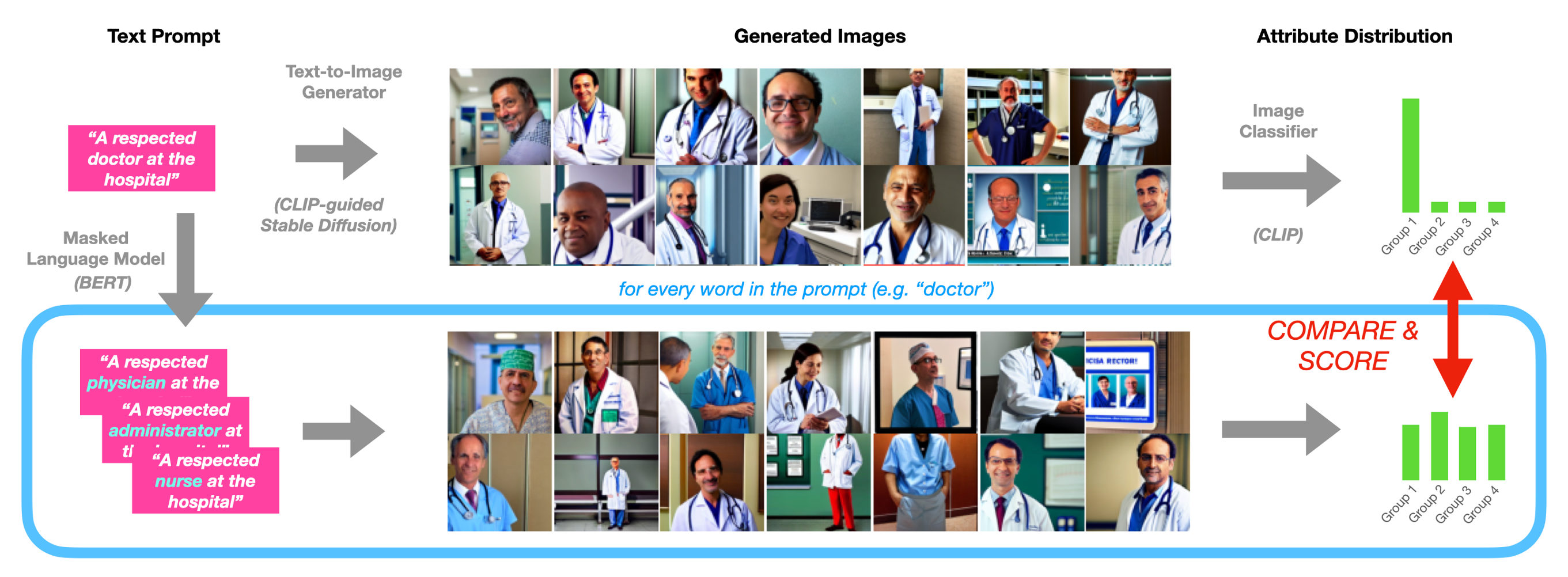
Figure 1: The diagram showing the proposed pipeline for the input prompt “A respected doctor at the hospital”.

Problem Setup and Notation. Let $p=p_{1},p_{2},\ldots,p_{k}\in\mathcal{P}$ denote a text prompt (sentence) comprised of words $p_{1},p_{2},\ldots,p_{k}$ where $k$ is the number of words in the prompt. A text-to-image generative model is denoted by T2I, i.e., $\textsc{T2I}(p)$ is a generated sample from a distribution of images $\mathbb{x}\in\mathcal{X}$ as a function of the prompt $p$. Moreover, let a sensitive attribute (e.g., sex, race, and age) of a person in an image be given by $\mathcal{G}(\mathbb{x})\in\{\mathbb{g}_{1},...,\mathbb{g}_{l}\}\triangleq\mathbb{G}$ – e.g., the sex of a person in the image $\mathbb{x}$. Finally, $\Pr_{T2I(p)}[\mathcal{G}(X)=\mathbb{g}]$ denotes the probability of the sensitive attribute of the generated images to be $\mathbb{g}$.

Word impact on representativeness. We start by considering the original prompt “A respected doctor at the hospital” showed in Fig. 1. Using CLIP-guided Stable Diffusion, this prompt generates images that are mostly males. However, the biased group distribution may be a consequence of the words “respected”, “doctor,” or even “ hospital,” next, we analyze which word is responsible for it.

To understand the impact of each word in the group distribution of the generated images, ideally, we would remove words from the prompt and analyze how this changes the sex of the produced images – as in explaining by removing (Covert et al., 2021). However, word removal may lead to sentences that are not grammatically coherent. For example, by removing the word “doctor,” the original prompt becomes “A respected at the hospital” – this sentence has no grammatical coherence. Therefore, we will replace each word with multiple other candidates generated by BERT (Devlin et al., 2018). BERT ensures that the sentence with replaced word has a rough grammatical coherence.

In Fig. 1, we show the images generated by the T2I model when we replace the word “doctor” in the original prompt with other words such as “physician,” “administrator,” and “nurse.” By replacing “doctor” the sex of the model generates images has more representativiness. Therefore, we ask the question How does the group distribution change when we replace certain words in the original prompt? To answer this question, we compare the distribution of the original prompt with the distribution of groups generated by the modified prompt. To make this comparison, it is necessary to have a systematical method to generate group distributions from a given (and transmuted) prompts. Next, we propose a method to do so.

Proposed Pipeline. We define a pipeline to (i) generate coherent transmuted prompts, (ii) sample images using the prompts, and (iii) attribute each image to a sensitive group. Our pipeline has three components, illustrated in Fig. 1.

1. Text Transmuter: We use a pretrained masked language model (MLM) to replace words in the original prompt. The MLM will substitute a word that is different from the original one, but still roughly obeys grammatical rules and completes the text in a sensical manner. In our implementation, we use a BERT-base MLM (Devlin et al., 2018).

2. Image Generator: Next, we pass each of the candidate prompts (the prompt with a replaced word) through the image generator and sample one image per prompt. This set of samples captures the distribution of images conditioned on removal the $i$-th word. Thus, it provides a counterfactual image distribution (i.e. what would have happened if word $i$ did not exist in the original prompt). Here we use CLIP-guided Stable Diffusion (Rombach et al., 2022) for image generation.

3. Group Classifier: Finally, we use a classifier that takes an image $\mathbb{x}$ as input and classifies it as a member of a group $\mathbb{g}$. In our pipeline, we use CLIP as a classifier by assigning $\mathbb{x}$ to the group that maximizes the CLIP score $\mathbb{g}=\arg\max_{\mathbb{g}^{\prime}\in\mathbb{G}}\text{CLIP}(\mathbb{x},\texttt{text}(\mathbb{g}^{\prime}))$, where $\texttt{text}(\mathbb{g}^{\prime})$ means to write $\mathbb{g}^{\prime}$ as a text string (e.g. “male” or “female”).

Our pipeline is model-agnostic and not restricted to the particular model choices we made here. With our proposed pipeline, we have access to the group membership distribution of the generated images. Hence, we are able to measure the importance of each word in the representativeness – next we define the word influence.

Word influence. We define a word-influence score $TI^{\mathcal{G}}(p,i,\mathbb{g}):\mathcal{P}\times[k]\times\mathbb{G}\rightarrow\mathbb{R}$. Intuitively, this word-influence score formalized in Definition 1 quantifies how much each word $p_{i}$ is responsible for producing the property $\mathcal{G}(\mathbb{x})=\mathbb{g}$ within the images generated by the prompt $p$. If $TI^{\mathcal{G}}(p,i,\mathbb{g})>TI^{\mathcal{G}}(p,j,\mathbb{g})$ the word $p_{i}$ influences more $\mathcal{G}(\mathbb{x})$ than $p_{j}$ for the prompt $p$. When $\mathcal{G}$ is clear from the context, we denote $TI^{\mathcal{G}}(p,i,\mathbb{g})$ by $TI(p,i,\mathbb{g})$.

We denote the probabilities of a generated image being part of a given group $\mathbb{g}$ by:

$$P_{\mathcal{S}}(\mathbb{g}) \triangleq\Pr_{\textsc{T2I}(\textsc{BERT}(p_{/\mathcal{S}}))}[\mathcal{G}(X)=\mathbb{g}]$$

$$P_{\mathcal{S}\cup\{i\}}(\mathbb{g}) \triangleq\Pr_{\textsc{T2I}(\textsc{BERT}(p_{/\mathcal{S}\cup\{i\}}))}[\mathcal{G}(X)=\mathbb{g}]$$

where $\text{BERT}(p_{/\mathcal{S}})$ means to replace the words corresponding to subset $\mathcal{S}$ using BERT (Devlin et al., 2018). Next, we define the word Influence Score.

Definition 1 (word Influence for group $\mathbb{g}$).

Given a prompt $p$ with $k\in\mathbb{N}^{+}$ words, we define the $r$-level influence of word $i\in[k]$ for the group $\mathbb{g}$ as:

$$TI(p,i,r,\mathbb{g})\triangleq\sum_{\begin{subarray}{c}\mathcal{S}\subseteq[k]\\ i\not\in\mathcal{S}\\ |\mathcal{S}|\leq r-1\end{subarray}}\frac{P_{\mathcal{S}}(\mathbb{g})-P_{\mathcal{S}\cup\{i\}}(\mathbb{g})}{{k-1\choose|\mathcal{S}|}},$$ (1)

SHAP values inspired our definition for the word influence (Lundberg & Lee, 2017).

Measuring Word influence. At first, our definition of the word influence score may seem impractical because it is a function of the group probability distribution, which is unknown – imagine knowing the race distribution of images generated by a large language model. However, the word influence score may be approximated by generating multiple images using the same prompt. We show in Theorem 1 that our estimation for the word-influence converges exponentially fast to the true word-influence score.

For each distribution $P_{\mathcal{S}}$ and $P_{\mathcal{S}\cup\{i\}}$ we sample $m$ i.i.d. images and denote the empirical distribution of $\mathbb{g}$ in the images $\hat{P}_{\mathcal{S}}(\mathbb{g})$ and $\hat{P}_{\mathcal{S}\cup\{i\}}(\mathbb{g})$ – see appendix for details. With this, we define the approximation for the word-influence for group $\mathbb{g}$ as:

$$\widehat{TI}(p,i,r,\mathbb{g})=\sum_{\begin{subarray}{c}\mathcal{S}\subseteq[k]\\ i\not\in\mathcal{S}\\ |\mathcal{S}|\leq r-1\end{subarray}}\frac{\hat{P}_{\mathcal{S}}(\mathbb{g})-\hat{P}_{\mathcal{S}\cup\{i\}}(\mathbb{g})}{{k-1\choose|\mathcal{S}|}}$$ (2)

Theorem 1 (Shap Word Influence Concentrates).

Let $\widehat{TI}(p,i,r,\mathbb{g})$ be the estimator for the word-influence defined in (2). If the sampled images are i.i.d. using the image generator for the prompts $P_{\mathcal{S}}$ and $P_{\mathcal{S}\cup\{i\}}$ then:

$$\Pr[|\widehat{TI}(p,i,r,\mathbb{g})-{TI}(p,i,r,\mathbb{g})|>t]\leq O(e^{-m})$$ (3)

Now that we have shown that it is possible to estimate the word-influence in Definition 1 via resampling images, in the next section, we show empirical results using this metric.

3 Experimental Results

A Detailed First Example. Consider the prompt “a respected doctor at the hospital”. Figure 1 shows that by using Stable Diffusion, the majority of generated images contain male individuals. Using our pipeline we can detect which words in the input prompt contribute to the underrepresentation of females given by Table 1. From the word influence calculated for each word, we observe that the word “doctor” has the highest score for male, followed by “respected”. The word “hospital” has slight female bias. The prepositions and articles (e.g. “at”, “the”, “a”) have negligible scores because they do not affect the semantic meaning of the sentence – see appendix 2 for examples of text transmutations.

Prompt ($p$)	$P(\text{Female}|p)$	word Influence
Original Prompt	0.160	—–
Prompt without “a”	0.133	-0.027
Prompt without “respected”	0.267	+0.107
Prompt without “doctor”	0.533	+0.373
Prompt without “at”	0.200	+0.040
Prompt without “the”	0.200	+0.040
Prompt without “hospital”	0.000	-0.160

Table 1: Word influence for each word and the probability of being classified as female for the original prompt “a respected doctor at the hospital” and replacing each word.

The Effect of Multiple Shapley Levels. We now provide a second example to demonstrate the utility of computing $r$-level word influence scores for $r>1$. As explained in Section 2, this is inspired by a connection to the Shapley values framework (Lundberg & Lee, 2017). We consider the following prompt: “the ceo of a fortune 500 company”.

Figure 2 (left) presents $r=1$-level word influence scores for this prompt, following the same setup as that of Section 3. We observe that all words have zero influence score. This is because (i) the original prompt only generates male images and (ii) no matter which single word is removed from the original prompt, the remaining words still carry a heavy male bias, so the sex distribution does not change. Thus, $r=1$ leads to uninformative scores for this prompt.

In contrast, Fig. 2 (right) presents $r=2$-level word influence scores for the same prompt, which considers replacement of all subsets of size $\leq 2$. We observe that some words have non-zero scores. Notably, the words “ceo” and “company” have the largest effect on the sex of the images being male. This indicates that replacing multiple words in the input prompt produces more informative scores by considering complex interactions between words. However, increasing $r$ also leads to higher computational costs.

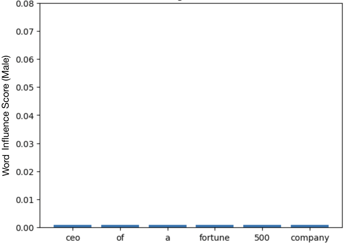
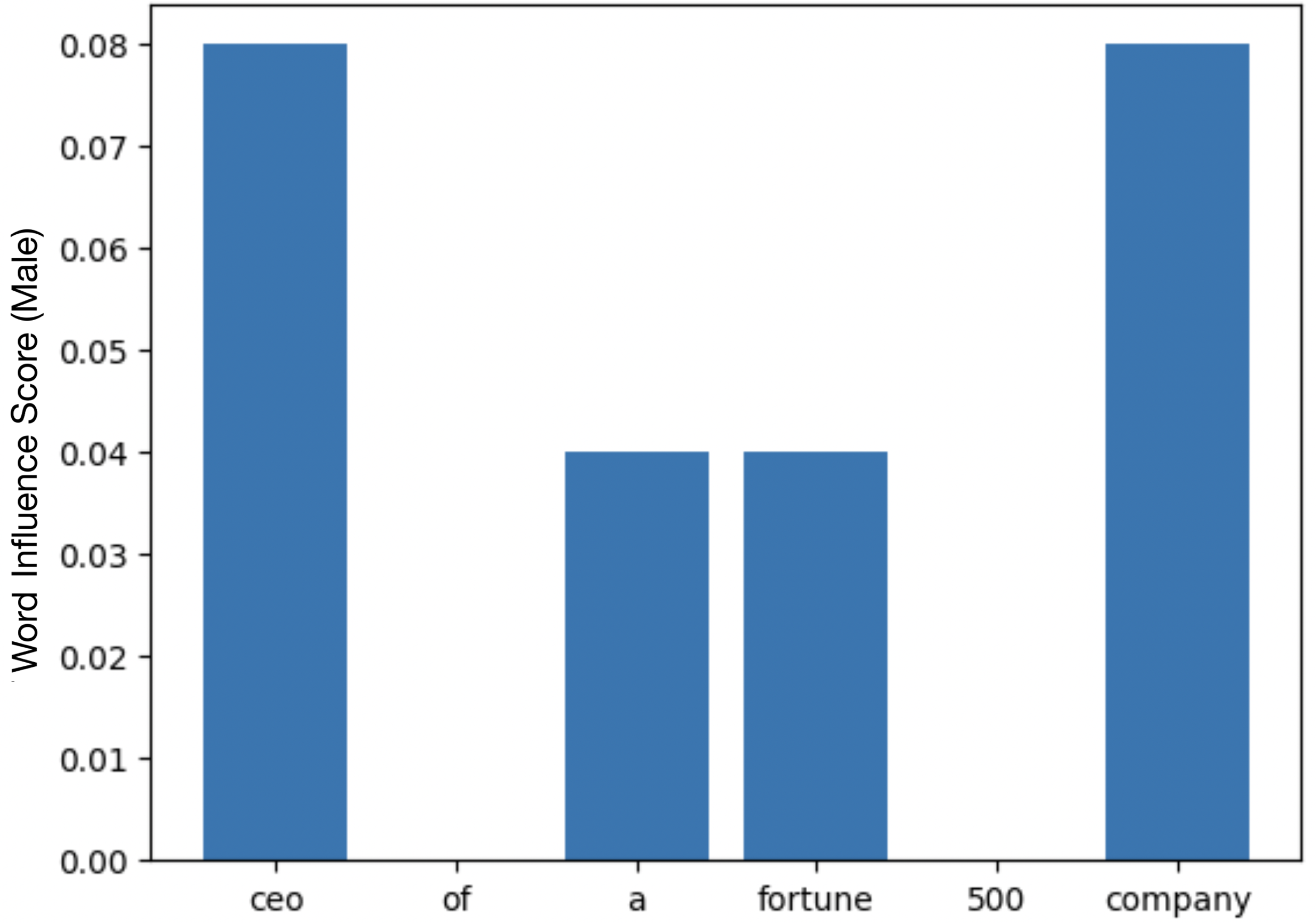
Figure 2: Word influence per word in the input prompt ”ceo of a fortune 500 company” using $(r=1)$ (left) and $(r=2)$ (right) as in Definition 1.

Large-Scale Evaluation. Finally, we test our pipeline on a collection of prompts to demonstrate how insights on model bias can be extracted. We create 150 prompts with the following structure: “a [ADJECTIVE] [PERSON] at the [PLACE]” (e.g., “a confident doctor at the mall”) where values for [ADJECTIVE], [PERSON], and [PLACE] are given in the Appendix. For each prompt, our pipeline gives influence scores for every word. In Figure 3, we show the average influence score across all prompts containing that word. We observe that words such as “nurse”, “caring”, “sensitive”, and “salon” are associated with female, i.e., their inclusion in the prompt leads to the generation of female images. Similarly, the words “doctor”, “scientist”, “confident”, and “rational” lead to the generation of male images.

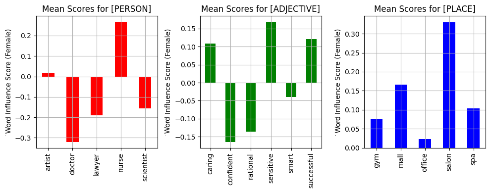
Figure 3: Averaged word influence scores for the words [PERSON] (left), [ADJECTIVE] (center), and [PLACE] (right) across all prompts in the large-scale evaluation.

4 Final Discussion

Conclusion. There are growing concerns that text-to-image (T2I) systems perpetuate and amplify stereotypes about minorities. In this work, we provide a method to calculate the relative importance of each word for the representativeness of individuals with a given sensitive attribute. Specifically, given a prompt and a text-to-image model, our approach assigns a score to each word in the prompt, representing its impact on the number of images of individuals with a given sensitive attribute. Moreover, our approach can be used to study if a T2I model associates sensitive attributes to words that are agnostic to them. Our results indicate that Stable Diffusion associates words like “scientist” and “lawyer” with males while associating “salon” and “sensitive” with females.

Limitations. While our proposed pipeline admits any text transmutation algorithm, define the best way to generate them is still an open question. In this paper, we use BERT to generate replacement candidates for each word. Alternative approaches are (i) the use of other masked language models, (ii) considering all possible syntactically correct word candidates, and (iii) an exhaustive list of synonyms and antonyms as word replacements.

Appendix A Appendix

Approximation of the Word Influence Score

We define the empirical probabilities to approximate the word influence in section 2 as:

$$\widehat{\Pr}_{\textsc{T2I}(\textsc{BERT}(p_{/\mathcal{S}}))}[\mathcal{G}(X)=g] \triangleq\frac{1}{m}\sum_{j=1}^{m}1_{\mathcal{G}(X_{j}^{/\mathcal{S}})=\mathbb{g}}$$ (4)

$$\widehat{\Pr}_{\textsc{T2I}(\textsc{BERT}(p_{/\mathcal{S}\cup\{i\}}))}[\mathcal{G}(X)=g] \triangleq\frac{1}{m}\sum_{j=1}^{m}1_{\mathcal{G}(X_{j}^{/\mathcal{S}\cup\{i\}})=\mathbb{g}},$$ (5)

where $1_{f(x)=\mathbb{g}}=1$ if $f(x)=\mathbb{g}$ and $0$ otherwise.

Proof of Theorem 1

Proof.

$$\Pr[|\widehat{TI}(p,i,r,\mathbb{g})-{TI}(p,i,r,\mathbb{g})|>t]$$

$$=\Pr[|\sum_{\begin{subarray}{c}\mathcal{S}\subseteq[k]\\ i\not\in\mathcal{S}\\ |\mathcal{S}|\leq r-1\end{subarray}}\frac{\widehat{\Pr}_{\textsc{T2I}(\textsc{BERT}(p_{/\mathcal{S}}))}[\mathcal{G}(X)=g]-\widehat{\Pr}_{\textsc{T2I}(\textsc{BERT}(p_{/\mathcal{S}\cup\{i\}}))}[\mathcal{G}(X)=g]}{{k-1\choose|\mathcal{S}|}}-{TI}(p,i,r,\mathbb{g})|>t]$$

For simplicity, denote $\widehat{\Pr}_{\textsc{T2I}(\textsc{BERT}(p_{/\mathcal{S}}))}[\mathcal{G}(X)=g]$ by $\widehat{P}_{\mathcal{S}}$ and $\widehat{\Pr}_{\textsc{T2I}(\textsc{BERT}(p_{/\mathcal{S}\cup\{i\}}))}[\mathcal{G}(X)=g]$ by $\widehat{P^{*}}_{\mathcal{S}}$. Therefore, we can write:

$$\Pr[|\widehat{TI}(p,i,r,\mathbb{g})-{TI}(p,i,r,\mathbb{g})|>t]$$

$$=\Pr[|\sum_{\begin{subarray}{c}\mathcal{S}\subseteq[k]\\ i\not\in\mathcal{S}\\ |\mathcal{S}|\leq r-1\end{subarray}}\frac{\widehat{P}_{\mathcal{S}}-\widehat{P^{*}}_{\mathcal{S}}-{P}_{\mathcal{S}}+{P^{*}}_{\mathcal{S}}}{{k-1\choose|\mathcal{S}|}}>t]$$

$$\leq\sum_{\begin{subarray}{c}\mathcal{S}\subseteq[k]\\ i\not\in\mathcal{S}\\ |\mathcal{S}|\leq r-1\end{subarray}}\Pr[|\frac{\widehat{P}_{\mathcal{S}}-\widehat{P^{*}}_{\mathcal{S}}-{P}_{\mathcal{S}}+{P^{*}}_{\mathcal{S}}}{{k-1\choose|\mathcal{S}|}}>\frac{t}{(\sum_{|\mathcal{S}|}{k-1\choose|\mathcal{S}|})}]$$

$$\leq\sum_{\begin{subarray}{c}\mathcal{S}\subseteq[k]\\ i\not\in\mathcal{S}\\ |\mathcal{S}|\leq r-1\end{subarray}}\Pr[|\frac{\widehat{P}_{\mathcal{S}}-{P}_{\mathcal{S}}}{{k-1\choose|\mathcal{S}|}}>\frac{t}{2(\sum_{|\mathcal{S}|}{k-1\choose|\mathcal{S}|})}]+\Pr[|\frac{\widehat{P}_{\mathcal{S}}^{*}-{P}_{\mathcal{S}}^{*}}{{k-1\choose|\mathcal{S}|}}>\frac{t}{2(\sum_{|\mathcal{S}|}{k-1\choose|\mathcal{S}|})}]$$

$$\leq 4\sum_{\begin{subarray}{c}\mathcal{S}\subseteq[k]\\ i\not\in\mathcal{S}\\ |\mathcal{S}|\leq r-1\end{subarray}}\exp^{-\frac{t^{2}m{k-1\choose|\mathcal{S}|}^{2}}{(\sum_{|\mathcal{S}|}{k-1\choose|\mathcal{S}|})^{2}}}$$

Where the last inequality comes from Hoeffding’s inequality. ∎

Masked Word	Transmutation
A	the respected doctor at the hospital
	highly respected doctor at the hospital
	well respected doctor at the hospital
respected	a staff doctor at the hospital
	a female doctor at the hospital
	a retired doctor at the hospital
doctor	a respected physician at the hospital
	a respected surgeon at the hospital
	a respected official at the hospital
hospital	a respected doctor at the university
	a respected doctor at the clinic
	a respected doctor at the time

Table 2: Example transmutations for the prompt ”A respected doctor at the hospital”

CLIP Classifier on CelebA

CelebA (Celebrities Attributes) (Liu et al., 2015) is a large-scale face attribute dataset containing over 200,000 celebrity images, each with 40 attribute annotations including sex, age, facial expression, and more. The sex attribute takes one of two possible values: ”Male” or ”Female”. Following is the classification report of CLIP classifier on CelebA dataset. The results 3 of this experiment suggest that CLIP when used as a sex classifier is fairly accurate.

Class	Precision	Recall	F1 Score	Support
female	0.97	1.00	0.98	94509
male	1.00	0.96	0.98	68261
accuracy			0.98	162770
macro average	0.98	0.98	0.98	162770
weighted average	0.98	0.98	0.98	162770

Table 3: Performance of CLIP classifier on sex attribute of CelebA dataset

CLIP Classifier on generated images

We also benchmark CLIP classifier against a pre-trained image classification model DeepFace (Serengil & Ozpinar, 2020) with two labels (’male’ and ’female’). As we are interested in CLIP’s performance on generated images, we run the classifiers on images generated with the prompt ”a respected doctor at the hospital” and it’s transmutations. Furthermore, a generated image could have multiple people, hence, we first pass the image through an object detector (Fang et al., 2021) to identify the bounding boxes of people, and run both the classifiers on cropped bounding boxes. The results are shown in Table 4. We can see that CLIP as a classifier is consistent with other image classifiers, suggesting that CLIP is largely unbiased, and the observed bias lies in the image generation process.

Class	Precision	Recall	F1 Score	Support
female	0.36	0.92	0.52	13
male	0.99	0.83	0.91	127
accuracy			0.84	140
macro average	0.68	0.88	0.71	140
weighted average	0.93	0.84	0.87	140

Table 4: Performance of CLIP as a classifier and DeepFace on generated images with the prompt ”a well respected doctor at the hospital”. Note that the support for male and female images is vastly different due to the bias in generation process.

Values for Placeholder in Large-Scale Evaluation (Section 2)

[ADJECTIVE] is a placeholder for one of $\{$“confident”, “caring”, “rational”, “sensitive”, “smart”, “successful”$\}$; [PERSON] is a placeholder for one of $\{$“doctor”, “scientist”, “artist”, “nurse”, “lawyer”$\}$; and [PLACE] is a placeholder for one of $\{$“office”, “gym”, “salon”, “spa”, “mall”$\}$.

References

- An & Kwak (2019) An, J. and Kwak, H. Gender and racial diversity in commercial brands’ advertising images on social media. In Social Informatics, Lecture Notes in Computer Science. Springer, 2019.
- Bianchi et al. (2022) Bianchi, F., Kalluri, P., Durmus, E., Ladhak, F., Cheng, M., Nozza, D., Hashimoto, T., Jurafsky, D., Zou, J., and Caliskan, A. Easily accessible text-to-image generation amplifies demographic stereotypes at large scale, 2022.
- Chambon et al. (2022) Chambon, P., Bluethgen, C., Langlotz, C., and Chaudhari, A. Adapting pretrained vision-language foundational models to medical imaging domains. arXiv preprint arXiv:2210.04133, 2022.
- Cho et al. (2022) Cho, J., Zala, A., and Bansal, M. Dall-eval: Probing the reasoning skills and social biases of text-to-image generative transformers. arXiv preprint arXiv:2202.04053, 2022.
- Covert et al. (2021) Covert, I., Lundberg, S., and Lee, S.-I. Explaining by removing: A unified framework for model explanation, 2021.
- Devlin et al. (2018) Devlin, J., Chang, M.-W., Lee, K., and Toutanova, K. Bert: Pre-training of deep bidirectional transformers for language understanding. arXiv preprint arXiv:1810.04805, 2018.
- Fang et al. (2021) Fang, Y., Liao, B., Wang, X., Fang, J., Qi, J., Wu, R., Niu, J., and Liu, W. You only look at one sequence: Rethinking transformer in vision through object detection. CoRR, abs/2106.00666, 2021. URL https://arxiv.org/abs/2106.00666.
- Fraser et al. (2023) Fraser, K. C., Kiritchenko, S., and Nejadgholi, I. Adapting pretrained vision-language foundational models to medical imaging domains. In AAAI 2023 Workshop creativeAI homepage, 2023.
- Johnson (2022) Johnson, K. Dall-e 2 creates incredible images—and biased ones you don’t see, 2022.
- Langley (2000) Langley, P. Crafting papers on machine learning. In Langley, P. (ed.), Proceedings of the 17th International Conference on Machine Learning (ICML 2000), pp. 1207–1216, Stanford, CA, 2000. Morgan Kaufmann.
- Liu et al. (2015) Liu, Z., Luo, P., Wang, X., and Tang, X. Deep learning face attributes in the wild. In Proceedings of International Conference on Computer Vision (ICCV), December 2015.
- Lundberg & Lee (2017) Lundberg, S. M. and Lee, S.-I. A unified approach to interpreting model predictions. Advances in neural information processing systems, 30, 2017.
- Midjourney (2022) Midjourney. Midjourney.com. www.midjourney.com, 2022.
- of Modern Art (2018) of Modern Art, T. M. Thinking machines: Art and design in the computer age, 1959-1989. 2018.
- Paiss et al. (2022) Paiss, R., Chefer, H., and Wolf, L. No token left behind: Explainability-aided image classification and generation. In Computer Vision–ECCV 2022: 17th European Conference, Tel Aviv, Israel, October 23–27, 2022, Proceedings, Part XII, pp. 334–350. Springer, 2022.
- Ramesh et al. (2021) Ramesh, A., Radford, A., Sordoni, A., and Bengio, D. Dall·e: Creating images from text. arXiv preprint arXiv:2102.12092, 2021.
- Ribeiro et al. (2016) Ribeiro, M. T., Singh, S., and Guestrin, C. ” why should i trust you?” explaining the predictions of any classifier. In Proceedings of the 22nd ACM SIGKDD international conference on knowledge discovery and data mining, pp. 1135–1144, 2016.
- Rombach et al. (2022) Rombach, R., Blattmann, A., Lorenz, D., Esser, P., and Ommer, B. High-resolution image synthesis with latent diffusion models. In Proceedings of the IEEE/CVF Conference on Computer Vision and Pattern Recognition, pp. 10684–10695, 2022.
- Serengil & Ozpinar (2020) Serengil, S. I. and Ozpinar, A. Lightface: A hybrid deep face recognition framework. In 2020 Innovations in Intelligent Systems and Applications Conference (ASYU), pp. 23–27. IEEE, 2020. doi: 10.1109/ASYU50717.2020.9259802. URL https://doi.org/10.1109/ASYU50717.2020.9259802.