The nonequilibrium evolution near the phase boundary

Abstract

We study the nonequilibrium evolution near the phase boundary of the 3D Ising model, and find that the average of relaxation time (RT) near the first-order phase transition line (1st-PTL) is significantly larger than that near the critical point (CP). As the system size increases, the average of RT near the 1st-PTL increases at a higher power compared to that near the CP. We further show that RT near the 1st-PTL is not only non-self-averaging, but actually self-diverging: relative variance of RT increases with system size. The presence of coexisting and metastable states results in a substantial increase in randomness near the 1st-PTL, making it difficult to achieve equilibrium.

I Introduction

Mapping the quantum chromodynamics (QCD) phase diagram is one of the physical objectives of current heavy ion collision experiments. The conjectured phase diagram consists of the first-order phase transition line (1st-PTL), the critical point (CP), and the crossover region QCD . Although the correlation length diverges at the phase boundary, the limited evolution time during heavy ion collisions makes it impossible for the correlation length to grow to infinity, leading to nonequilibrium phenomena near the phase boundary Berdnikov . Studying nonequilibrium phenomena near the phase boundary is of great significance for enriching phase transition theory itself and identifying the phase boundary in heavy ion collisions.

The nonequilibrium phenomenon near the CP was first studied 1977 . This is attributed to a property called critical slowing down. In the vicinity of the critical temperature $T_{\rm c}$, the autocorrelation time increases with the correlation length Newman . This increase follows a power-law with respect to the correlation length $\xi$ or the characteristic length of the lattice size $L$. The power exponent $z$, i.e. the dynamic critical exponent, describes the nonequilibrium dynamics 1977 ; MartinPRE . The value of $z$ of different systems were obtained and the main dynamic universality classes were identified 1977 .

At the 1st-PTL, the characteristics of nonequilibrium have not been understood as well as that of the CP. Initially, exponential slowing down was observed supercritical-1 ; supercritical-2 and referred to as supercritical slowing down, which resulted from deterioration in the simulation algorithm. By introducing the multicanonical algorithm, this type of slowing down was improved to follow a power-law. Subsequently, slowing down near the boundary of the coexisting region was observed in solutions of the dynamical mean-field theory of Mott-Hubbard transition JooPRB and later in mechanically induced adsorption-stretching transitions zhang2017 .

The slowing down phenomenon near the phase boundary is associated with the increase of randomness in the system which can be reflected by non-self-averaging property. As the system size increases, the relative variance of magnetization or susceptibility approaches a constant value, indicating non-self-averaging behavior at the CP non-selfaveraging-1 ; non-selfaveraging-2 ; non-selfaveraging-3 ; physicsA . Non-self-averaging behavior at the 1st-PTL has been observed only in the isotropic-to-nematic transition in liquid crystals nonSA-first-1 .

To fully present the dynamic properties in different regions of the phase boundary, it is necessary to study the nonequilibrium evolution near the entire phase boundary. The dynamical evolution is commonly described by the Langevin equation and various relaxation models, such as the kinetic Ising model kinetic-Ising or models A, B, C, etc., classified by the renormalization group 1977 . Initially, the dynamical solutions were limited to the crossover region Mukherjee , but later they were extended to include the 1st-PTL region langevin-sigma .

Recently, individual relaxation processes near the CP in the 3D Ising model have been simulated using the single-spin flipping dynamics XBLi . The relaxation time (RT) is defined as the number of sweeps required for the order parameter to reach its equilibrium value. It has been observed that the order parameter approaches its equilibrium value exponentially, which aligns with the behavior predicted by the Langevin equation and a mean-field approximation of relaxation in Ising model Glauber-analytical . To characterize the relaxation of a sample, the average of RT is introduced. It has been demonstrated that at the critical temperature, the average of RT follows a power-law increase with system size, and the dynamic exponent is consistent with the dynamic universality class of model A 1977 ; Roth . It indicates that the average of RT well represents the relaxation time in dynamical equations. Moreover, the third and fourth cumulants of the order parameter on the crossover side oscillate around zero, and then converge to their equilibrium values. The sign of the third cumulants can be negative, consistent with those obtained from dynamical equations Mukherjee ; Nahrgang . These facts suggest that the single-spin flipping dynamics can effectively describe the dynamical relaxation and provide an alternative method to explore nonequilibrium phenomena.

In this paper, we employ this method to investigate the nonequilibrium evolution near the phase boundary of the 3D Ising model. We begin by considering random initial configurations and present the average of RT on the phase plane for a specific system size of $L=60$. Subsequently, we discuss the self-averaging properties of RT at the phase boundary. Furthermore, we provide and analyze the results obtained from starting the simulations with a high-temperature state and a polarized initial state. Finally, we conclude with a brief summary.

II Characteristics of nonequilibrium evolution

The CP of the 3D Ising model belongs to the $Z(2)$ symmetry group. Various physical systems exhibit the same universality class as the 3D Ising model. Examples include the liquid-gas transition nuclear-liquid-gas , magnetic transition magnetic , quark deconfinement, and chiral phase transition in QCD Stephanov ; chiral-Ising ; k4-non .

The 3D Ising model considers a three dimensional simple cubic lattice composed of $N=L^{3}$ spins, where $L$ is called the system size. The total energy of the system with a constant nearest-neighbor interaction $J$ placed in a uniform external field $H$ is

$$E_{\{s_{i}\}}=-J\sum_{\langle ij\rangle}s_{i}s_{j}-H\sum_{i=1}^{N}s_{i},\quad s_{i}=\pm 1.$$ (1)

The per-spin magnetization is

$$m=\frac{1}{N}\sum_{i=1}^{N}s_{i}.$$ (2)

It serves as the order parameter of the continuous phase transition at the critical temperature $T_{\rm c}=4.51$ tc-Ising , and below $T_{\rm c}$, there is a 1st-PTL at $H=0$.

Single-spin flipping dynamics, e.g. Metropolis algorithm Metropolis , as a local dynamics of Glauber type kinetic-Ising , is suitable for studying nonequilibrium evolution Metropolis-NE1 ; Metropolis-NE2 . Starting from an initial configuration, Metropolis algorithm flips one single spin at each step. Whether a spin flips depends on the acceptance probability $A({\boldsymbol{u}}\rightarrow{\boldsymbol{v}})$, which is given by

$$A({\boldsymbol{u}}\rightarrow{\boldsymbol{v}})=\left\{\begin{array}[]{ll}e^{-(E_{\boldsymbol{v}}-E_{\boldsymbol{u}})/k_{\rm B}T}&\text{if $E_{\boldsymbol{v}}-E_{\boldsymbol{u}}>0$},\\ 1&\text{otherwise.}\end{array}\right.$$ (3)

${\boldsymbol{u}}$ and ${\boldsymbol{v}}$ represent the state of the system before and after flipping this spin. If $A({\boldsymbol{u}}\rightarrow{\boldsymbol{v}})=1$, the spin is flipped. If $A({\boldsymbol{u}}\rightarrow{\boldsymbol{v}})<1$, a random number $r$ ($0<r<1$) is generated. If $A({\boldsymbol{u}}\rightarrow{\boldsymbol{v}})>r$, the spin is flipped, otherwise, the spin keeps its original state. The testing of one single spin is called a Monte Carlo step. When $N$ Monte Carlo steps are completed, every spin in the lattice has been tested for flipping and one sweep is completed. In this way, the configuration of the system is updated once a sweep. Relaxation time of a process is defined by the number of sweeps required for magnetization to reach a stable value XBLi .

To quantify the RT of a sample, the average of RT is suggested as XBLi ,

$$\bar{\tau}=\frac{1}{n}\sum_{i=1}^{n}\tau^{i},$$ (4)

where $n$ is the total number of evolution processes, $\tau^{i}$ is RT of the $i^{\rm th}$ process.

Figure 1 presents a contour plot of the average of RT on the $T$-$H$ phase plane for a fixed system size of $L=60$, starting from random initial configurations. The color scheme ranges from white to red to black, representing the average of RT values that span from less than a hundred to over four thousand. The phase boundary is depicted by the line $H=0$. In regions far from the phase boundary, the color appears light, indicating a small average of RT. However, a dark-red point emerges around $T_{\rm c}=4.51$, indicating a large average of RT, which is consistent with the phenomenon of critical slowing down as expected.

Figure 1: A contour plot of the average of RT on the phase plane of the 3D Ising model for $L=60$.

Along the 1st-PTL, the color becomes progressively darker as the temperature decreases, eventually turning completely black when the temperature drops below 4.2. Simultaneously, on the low-temperature side, specifically along the direction of the external field, the color transitions rapidly to black near $H=0$. These observations indicate that the relaxation process near the 1st-PTL is considerably slower than that near the CP, and can be characterized as ultra-slowing down.

Ultra-slowing down indicates a higher level of uncertainty and randomness. This can be attributed to the more complex structure of the free energy at the 1st-PT compared to the CP. The 1st-PT represents a transition between distinct internal states, where both upward and downward magnetized phases coexist along the transition line. In the equilibrium state, the system can be either in an upward or downward magnetized state with equal probability, effectively doubling the number of possible states. Near the 1st-PTL, some of these possible states manifest as metastable states, as indicated by the spinodal curve JooPRB ; Binder . The presence of coexisting and metastable states significantly increases the instability, uncertainty, and randomness in the equilibrium state. This heightened randomness results in a much longer RT. Consequently, achieving equilibrium at the 1st-PT is a challenging task.

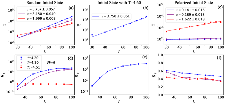
Figure 2: The finite size scaling of the average of RT for three different initial states: random initial state (a), equilibrium state at $T=4.60$ (b), and polarized initial state (c). $R_{\tau}$ as a function of $L$ for each of these cases, denoted as (d), (e), and (f) respectively.

To show the system size dependence of a nonequilibrium evolution, Fig. 2(a) presents a double-logarithmic plot illustrating the variation of the average of RT with system size for three different temperatures at the boundary. The data points corresponding to $T_{\rm c}=4.51$ are denoted by red squares, while the data points below $T_{\rm c}$ are represented by blue circles and purple triangles. The error bars indicate only the statistical errors.

Both at the CP and the 1st-PTL, the average of RT increases with system size, and can be accurately described by a power-law relationship, i.e.,

$$\bar{\tau}\propto L^{z}.$$ (5)

The power exponent $z$, which corresponds to the slope of the fitting line, represents the dynamic exponent. The $z$ values are provided in the legend of Fig. 2(a). The critical dynamic exponent $z=1.999\pm 0.008$ is obtained by fitting from $L=20$ to $L=100$, which has higher statistics and is more precise than the previously reported value of $z=2.06\pm 0.03$ XBLi . Both values are consistent with the dynamic universality class of model A 1977 ; Roth . This shows that the average of RT, as defined by Eq. (4), serves as a similar role to the autocorrelation time. At the 1st-PTL, the dynamic exponent $z$ is larger than that at the CP. As a result, the average of RT at the 1st-PTL increases more rapidly with system size than that at the CP.

To further investigate the change in the randomness of the RT with system size, we examine its self-averaging property. Self-averaging refers to the behavior of the relative variance of an observable $X$ as the system size increases. It is defined as follows non-selfaveraging-1 :

$$R_{X}=\frac{\overline{X^{2}}-\overline{X}^{2}}{\overline{X}^{2}},$$ (6)

where bar represents the average over the entire sample. If $R_{X}$ tends to zero, $X$ is self-averaging; if $R_{X}$ increases, $X$ is self-diverging. In case of self-averaging, the fluctuation of $X$ diminishes as the system size increases, and the average of $X$ converges to the same value. Self-diverging means divergent fluctuations of $X$ as the system size increases.

At the phase boundary, the relative variance of $\tau$ is plotted against the system size for three different temperatures in Fig. 2(d). The trend of $R_{\tau}$ with system size is observed to be significantly different for each temperature. Notably, at the critical temperature $T_{\rm c}=4.51$, $R_{\tau}$ remains almost constant as the system size increases. In other words, the variance or width of the RT distribution increases with the system size at the same rate as the average of RT, indicating non-self-averaging behavior of RT. This observation is consistent with other observables studied in the same context non-selfaveraging-1 .

At temperatures $T=4.30$ and $T=4.20$, it is observed that $R_{\tau}$ increases with system size, indicating self-diverging behavior at the 1st-PTL. This behavior is similar to what is observed in liquid crystals nonSA-first-1 . As the system size increases, the variance of RT increases more rapidly than the average of RT, and the distribution of RT become wider and flatter. This phenomenon suggests that randomness is significantly amplified with system size, leading to an abnormally increased variance. Such an extremely broad distribution of RT is a characteristic feature of the relaxation near the 1st-PTL.

To explore the behavior away from the boundary, the average of RT is plotted against the system size in a double-logarithmic plot for three external fields at a specific temperature $T=4.2$ in Fig. 3(a). The external fields are $H=10^{-5}$ (red crosses), $H=0.001$ (blue triangles), and $H=0.02$ (green squares). Figure 3(a) illustrates that for each external field, as the system size increases, the average of RT also increases and can be fitted by a line, similar to the case shown in Fig. 2(a). Consequently, away from the boundary, the average of RT exhibits a power-law relationship with system size.

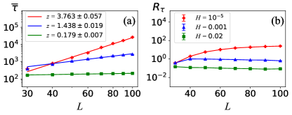
Figure 3: (a) The finite size scaling of the average of RT for three different values of the external magnetic field at $T=4.20$. (b) The relative variance of RT as a function of system size for each of the aforementioned cases.

The power $z$ for $H=10^{-5}$ as presented in the legend of Fig. 3(a) is nearly the same as that observed at the 1st-PTL shown in Fig. 2(a). However, as one moves away from the 1st-PTL along the direction of the external magnetic field, $z$ gradually decreases. This reduction can be attributed to the alignment tendency of spins with the external magnetic field. As the external field becomes non-zero, the spins tend to align in the direction of the field, thereby reducing the overall randomness in the system.

Furthermore, similar to the case presented in Fig. 3(a), the relative variance $R_{\tau}$ is plotted against the system size for three external fields in Fig. 3(b). It is observed that self-diverging behavior is only prominent at $H=10^{-5}$, which is the nearest to the 1st-PTL. For larger external fields, such as $H=0.001$ and $H=0.02$, $R_{\tau}$ decreases slowly as $L$ increases, indicating self-averaging of RT. As the deviation from the 1st-PTL becomes further, the self-diverging behavior of RT becomes less pronounced. Therefore, self-diverging behavior is observed not only precisely at the 1st-PTL but also in its close vicinity, while far from the phase boundary, RT exhibits self-averaging behavior.

As demonstrated in Ref. XBLi , the initial configuration has a significant impact on the RT. A random initial configuration represents a completely disordered state, indicating a very high temperature. Nonequilibrium evolution from such a high temperature state to the phase boundary can occur spontaneously. To provide a comprehensive analysis, we also include the results for initial states with a temperature of $T=4.6$ and a polarized configuration.

The initial configuration of Figs. 2(b) and 2(e) corresponds to an equilibrium configuration at $T=4.6$, while the final state temperature is $T=4.2$. Both configurations lie on the boundary $H=0$. It is evident that the initial state with $T=4.6$ is less random than, but still very close to, the random initial configuration. The average of RT shown in Fig. 2(b) also exhibits an increase with system size and can be fitted with a straight line, similar to Fig. 2(a), but with a slightly smaller $z$. Therefore, the divergence of average of RT is not as rapid as in Fig. 2(a) due to the reduced randomness. Simultaneously, the relative variance of RT, as shown in Fig. 2(e), also increases with system size, indicating the occurrence of self-diverging RT.

Figures 2(c) and 2(f) present the average and the relative variance of RT from a polarized initial configuration. In Fig. 2(c), the average of RT increases with system size for each temperature and can be fitted with a line. The slope $z$ at the critical temperature is the largest but smaller than that in Fig. 2(a). The slopes $z$ for the other two temperatures decrease significantly compared to Fig. 2(a). Additionally, Fig. 2(f) demonstrates that the relative variance of RT decreases with system size for all three temperatures, indicating that RT exhibits self-averaging behavior in this case.

As we know, a polarized initial configuration is equivalent to an equilibrium state at a very low temperature. This ordered state possesses a similar structure to the equilibrium states at the 1st-PTL. Consequently, the evolution from a polarized initial configuration to the states at the 1st-PTL is facile, resulting in a substantial reduction in the average of RT. The self-diverging behavior observed in Fig. 2(d) is completely absent. However, it should be noted that the structure of the polarized configuration still remains distinct from that of the CP. The average of RT towards the CP still diverges.

III Summary and discussion

In summary, the single-spin flipping dynamics has been employed to achieve nonequilibrium evolution from three different types of initial states to the phase boundary of the 3D Ising model.

We generate random initial configurations and plot the contour of average of RT on the phase plane for a fixed system size of $L=60$. In comparison to the critical slowing down, $\bar{\tau}$ near the 1st-PTL exhibits ultra-slowing down behavior. As the system size increases, $\bar{\tau}$ near the 1st-PTL follows a power-law increase, similar to the behavior near the CP, but with a larger dynamic exponent.

The self-averaging properties of RT at and near the phase boundary are also examined. As the system size increases, the relative variance of RT near the 1st-PTL increases, eventually converging to a constant value near the CP. Consequently, RT exhibits self-diverging behavior near the 1st-PTL, and non-self-averaging behavior near the CP. The level of randomness near the 1st-PTL is significantly higher than the CP. This increased randomness can be attributed to the presence of coexistence and metastable states, which greatly expand the number of possible states and consequently lead to a highly broad distribution of RT. This characteristic of relaxation near the 1st-PTL distinguishes it from the behavior observed at the CP.

While the specific value of the dynamic exponent can vary with the model and algorithm employed scaling-Fischer , the characteristics of nonequilibrium relaxation, such as ultra-slowing down and self-diverging at the 1st-PTL, critical slowing down and non-self-averaging, and power-law behavior with increasing system size, are expected to be general. They can be observed across different models and algorithms, providing insights into the universal behavior of systems near phase transitions.

These qualitative features are instructive in understanding the nonequilibrium effects near the phase boundary of the QCD phase diagram. As we know, nonequilibrium evolution near the CP alters the magnitude and even sign of the observables. Since the slowing down phenomenon of the 1st-PT is more severe than that of the CP, the nonequilibrium phenomena near the 1st-PTL is more complex and need more caution. Further research on the influences of nonequilibrium evolution on observables has great value in identifying the 1st-PTL in heavy ion collision experiments.

References

- (1) A. Bzdak, S. Esumi, V. Koch, J. Liao, M. Stephanov, N. Xu, Phys. Rep. 853, 1 (2020).
- (2) B. Berdnikov and K. Rajagopal, Phys. Rev. D 61, 105017 (2000).
- (3) P.C. Hohenberg and B.I. Halperin, Rev. Mod. Phys. 49, 435 (1977).
- (4) M. E. J. Newman and G. T. Barkema, Monte Carlo Methods in Statistical Physics (Oxford University Press, Oxford, 1999).
- (5) M. Hasenbusch, Phys. Rev. E 101, 022126 (2020).
- (6) B. A. Berg and T. Neuhaus, Phys. Rev. Lett. 68, 9 (1992).
- (7) B. Berg, arXiv:cond-max/9909236, published as Fields Institute Communications 26, 1 (2000).
- (8) J. Joo and V. Oudovenko, Phys. Rev. B 64, 193102 (2001).
- (9) S. Zhang, S. Qi, L. I. Klushin, A. M. Skvortsov, D. Yan, and F. Schmid, J. Chem. Phys. 147, 064902 (2017).
- (10) S. Wiseman and E. Domany, Phys. Rev. E 52, 3469 (1995).
- (11) A. Malakis and N.G. Fytas, Phys. Rev. E 73, 016109 (2006).
- (12) G. Parisi and N. Sourlas, Phys. Rev. Lett. 89, 257204 (2002).
- (13) K. A. Pronin, Physica A 596, 127180 (2022).
- (14) J.M. Fish, R.L.C. Vink, Phys. Rev. Lett. 105, 147801 (2010).
- (15) N. Menyhard and G. Odor, Brazilian Journal of Physics 30, 113 (2000).
- (16) S. Mukherjee, R. Venugopalan, and Y. Yin, Phys. Rev. C 92, 034912 (2015).
- (17) Lijia Jiang, Jingyi Chao, Eur. Phys. J. A 59, 30 (2023).
- (18) Xiaobing Li, Mingmei Xu, Yanhua Zhang, Zhiming Li, Yu Zhou, Jinghua Fu and Yuanfang Wu, Phys. Rev. C 105, 064904 (2022).
- (19) I. Tikader and M. Acharyya, arXiv:2305.10765.
- (20) J.V. Roth, L. von Smekal, arXiv:2303.11817.
- (21) M. Nahrgang, M. Bluhm, T. Schafer, and S. A. Bass, Phys. Rev. D 99, 116015 (2019).
- (22) J. B. Elliott et al. (ISiS Collaboration), Phys. Rev. Lett. 88, 042701 (2002).
- (23) D. E. Laughlin, Metallurgical and Materials Transactions A 50, 2555 (2019).
- (24) M. A. Stephanov, K. Rajagopal and E. Shuryak, Phys. Rev. Lett. 81, 4816 (1998).
- (25) J. Berges, K. Rajagopal, Nucl. Phys. B 538, 215 (1999).
- (26) M. A. Stephanov, Phys. Rev. Lett. 107, 052301 (2011).
- (27) A. L. Talapov and H. W. Blote, J. Phys. A: Math. Gen. 29, 5727 (1996).
- (28) N. Metropolis, A. W. Rosen bluth, M. N. Rosenbluth, A. H. Teller and E. Teller, J. Chem. Phys. 21, 1087 (1953).
- (29) C.-W. Liu, A. Polkovnikov and A. W. Sandvik, Phys. Rev. B 89, 054307 (2014).
- (30) M. Acharyya, Phys. Rev. E 56, 2407 (1997).
- (31) K. Binder, D.P. Landau, Phys. Rev. B 30, 1477 (1984).
- (32) T. Fischer et al., J. Phys.: Condens. Matter 22, 104123 (2010).