Reducing Communication for Split Learning by Randomized Top-$k$ Sparsification

Abstract

Split learning is a simple solution for Vertical Federated Learning (VFL), which has drawn substantial attention in both research and application due to its simplicity and efficiency. However, communication efficiency is still a crucial issue for split learning. In this paper, we investigate multiple communication reduction methods for split learning, including cut layer size reduction, top-$k$ sparsification, quantization, and L1 regularization. Through analysis of the cut layer size reduction and top-$k$ sparsification, we further propose randomized top-$k$ sparsification, to make the model generalize and converge better. This is done by selecting top-$k$ elements with a large probability while also having a small probability to select non-top-$k$ elements. Empirical results show that compared with other communication-reduction methods, our proposed randomized top-$k$ sparsification achieves a better model performance under the same compression level.

1 Introduction

In recent years, the protection of data privacy has become an important issue in machine learning. To date, many kinds of solutions have been proposed to solve the data privacy issue. Aside from cryptographic methods Mohassel and Rindal (2018); Wagh et al. (2019); Chen et al. (2021a), Federated Learning (FL) Li et al. (2020) and Split Learning (SL) Vepakomma et al. (2018) are two promising methods for privacy-preserving machine learning. While typical federated learning (also known as Horizontal Federated Learning, HFL) mainly focuses on horizontally distributed data, split learning is a simple and effective solution for vertically distributed data. However, although split learning achieves better efficiency than cryptographic methods Chen et al. (2022), the communication efficiency is still an important issue. In this paper, we focus on reducing the communication of split learning.

The basic idea of split learning is to divide the model into several parts, and each part is computed by a different participant (party). Since split learning only requires sharing the intermediate outputs or gradients, instead of the original input and label, it is considered somewhat privacy-preserving. We present the overview of a typical split learning model in Figure 1, where we consider a two-party case — input feature and label are held by two parties, i.e., feature owner and label owner. To train a model without directly revealing participants’ data, the model is split into a bottom model and a top model, held by the feature owner and the label owner, respectively. The last layer (output) of the bottom model is called the cut layer. We simply describe the training procedure of split learning below:

• Forward pass: the feature owner first feeds the sample features $X$ to the bottom model $M_{b}$, then gets the intermediate output $O_{b}=M_{b}(X,\theta_{b})$, where $\theta_{b}$ is the bottom model’s weight. The label owner fetches $O_{b}$, feeds it to the top model $M_{t}$, and then gets the final output $\hat{Y}=M_{t}(O_{b};\theta_{t})$.

• Backward pass: the label owner calculates the loss function $L(\hat{Y},Y)$, then computes the gradients $\partial L(\hat{Y},Y)/\partial\theta_{t}$ and $G_{b}=\partial L(\hat{Y},Y)/\partial O_{b}$. The former gradient is used to update the top model, and the latter is sent to the feature owner. The feature owner computes the jacobian matrix $\partial O_{b}/\partial\theta_{b}$. Then the gradient with respect to the bottom model’s parameters can be computed as $\left(\partial O_{b}/\partial\theta_{b}\right)^{T}G_{b}$, which is used to update the bottom model.

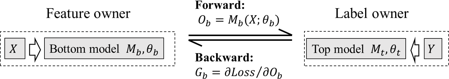
Figure 1: Overview of split learning.

However, despite its simplicity, the communication efficiency of split learning is still an important issue. During each iteration, the participants have to exchange intermediate results of the data batch, and the number of iterations and the size of intermediate results are usually large. For example, consider training ResNet-20 He et al. (2016) with the cut layer size equal to $32\times 32\times 32$ and batch size equal to 32. It takes 2 (forward & backward) $\times$ 4 (bytes for float value) $\times$ 32 (batch size) $\times 32^{3}$ (size of a single sample’s intermediate result) bytes = $8$ Mib traffic to finish a single iteration of inference, which is a huge communication cost, especially for mobile devices.

For federated learning, existing work has investigated different methods to reduce communication, including increasing local epochs McMahan et al. (2017), accelerating convergence Karimireddy et al. (2020); Wang et al. (2020a, b), and compressing local model updates in various ways Aji and Heafield (2017); Stich et al. (2018); Sattler et al. (2019b, a); Wang et al. (2018). For split learning, however, studies on communication reduction are relatively few. Castiglia et al. Castiglia et al. (2022) proved the convergence of compressing split learning by top-$k$ sparsification or quantization. Other methods such as asynchronous training, quantization, and using an autoencoder as a compressor are also investigated for specific tasks Chen et al. (2021b); Ayad et al. (2021).

In our work, we focus on reducing the communication for the classification problems with a large number of classes, and propose a modification of top-$k$ sparsification, namely, randomized top-$k$ sparsification (RandTopk). To perform randomized top-$k$ sparsification on a $d$-dimensional vector, we first determine its top-$k$ elements. Then we randomly select $k$ distinct elements such that: with probability $1-\alpha$, the element is chosen from top-$k$ elements with equal chance, and with probability $\alpha$, the element is chosen from non-top-$k$ elements with equal chance. Here, $\alpha\in[0,1]$ is a hyperparameter to control the randomness. The core idea behind randomized top-$k$ sparsification comes from the analysis of size reduction and top-$k$ sparsification. We find that when the number of classes is small (e.g. $\leq 10$), simply reducing the size of the cut layer can preserve model performance well. However, this does not hold when the number of classes is large (e.g. $\geq 100$), since hidden features of different classes will be crowded within a low-dimensional manifold, making the model less smooth and generalize poorly. Top-$k$ sparsification overcomes this problem by expanding the volume of the low-dimensional manifold. However, it still faces local minimum problems, and usually fails to exploit the entire volume of the manifold due to unevenly selected neurons, i.e., some neurons are selected frequently while some are rarely selected. RandTopk tackles both problems by adding randomness to top-$k$ sparsification. First, the local minimum can be avoided by noisy gradients; Second, since non-top-$k$ neurons also have chances to be selected during forward propagation, after training, the distribution of selected neurons is more balanced.

We conduct extensive experiments on different tasks, and compare RandTopk with top-$k$ sparsification, cut layer size reduction, quantization, and L1 regularization. Empirical results show that RandTopk significantly outperforms top-$k$ sparsification and other compression methods when their compression ratios are on the same level. We summarize our main contributions as follows:

• We investigate different compression methods for split learning to improve its communication efficiency, including cut layer size reduction, top-$k$ sparsification, quantization, and L1 regularization.

• Through the analysis of the cut layer size reduction and top-$k$ sparsification, we propose randomized top-$k$ sparsification, to overcome the convergence and generalization problems of top-$k$ sparsification.

• We conduct extensive experiments and show that randomized top-$k$ sparsification achieves the best model performance compared to other compression methods when their compression ratios are on the same level.

2 Related Work

2.1 Reducing Communication for HFL

A classic communication reduction method for HFL is the famous FedAvg scheme McMahan et al. (2017), which reduces communication rounds for HFL by letting client train more rounds locally, and has now become the standard HFL scheme. Based on this, studies aiming to reduce communication in HFL can be mainly divided into two classes, i.e., making convergence faster and compressing the model updates. Methods of the former class usually accelerate convergence by making model updates of different clients more consistent Wang et al. (2020a, b); Karimireddy et al. (2020); Jin et al. (2022). The latter class includes quantization, sparsification, and other compression methods. The basic top-$k$ sparsification is well-studied both empirically and theoretically and is proven to be very effective Aji and Heafield (2017); Stich et al. (2018). Combining sparsification and quantization can further reduce communication  Wen et al. (2017); Sattler et al. (2019b, a). Other methods, such as using SVD to compress the model updates Wang et al. (2018); Vogels et al. (2019) and using autoencoder as compressor Chandar et al. (2021), are also investigated.

2.2 Reducing Communication for VFL

As for VFL, the studies on communication reduction are relatively few. Castiglia et al. Castiglia et al. (2022) studied the convergence using top-$k$ sparsification and quantization. Other techniques like asynchronous training and autoencoder compressor are also used in specific tasks Chen et al. (2021b); Ayad et al. (2021). Chen et al. Chen et al. (2021b) use asynchronous training and quantization to reduce the communication for split learning. Using asynchronous training, the bottom model is not updated every iteration, hence the top model no longer needs to send the gradient to the bottom model in every iteration. The authors also show that this method neither enhances nor harms the privacy of split learning. Ayad et al. Ayad et al. (2021) use an autoencoder to compress the intermediate results. However, this method requires injecting an autoencoder which has to be specifically designed for different tasks.

3 Basic Compression for Split Learning

Notation	Definition
$M_{b},M_{t}$	The bottom model and the top model
$X$	Input instance
$O$	Output of the bottom model
$\hat{Y},Y$	Model prediction and label
$L(\hat{Y},Y)$	Loss function
$G_{o}$ or $G$	Gradient of the loss ($\partial L/\partial O_{b}$)
$\mathsf{Comp},\mathsf{Decomp}$	Compression/Decompression function
$\mathsf{Encode},\mathsf{Decode}$	Encode/Decode between values and bytes
$d$	Dimension of the bottom model output
$k$	#Non-zero elements after sparsification
$n$	Number of classes

Table 1: Notations & Definitions

In split learning, intermediate results are sent during each forward pass and backward pass. Hence, the compression is performed on the intermediate results. Specifically, in this paper, we only consider the compression on the instance level, i.e., if there is a batch of instances, the compression method is applied to the instances’ bottom model outputs inside the batch individually. Let $\mathsf{Comp}(\cdot):\mathbb{R}^{d}\to\mathbb{B}^{*}$ and $\mathsf{Decomp}(\cdot):\mathbb{B}^{*}\to\mathbb{R}^{d}$ be the compression and corresponding decompression operator, where $\mathbb{B}^{*}$ is the bytes array of arbitrary length. For simplicity, we denote $C[\cdot]\equiv\mathsf{Decomp}[\mathsf{Comp}(\cdot)]$. Note that the compression methods discussed in this paper usually are not lossless, hence $C[X]$ and $X$ are usually not equal. Let $X$ be an input instance, and we assume that the output of $M_{b}$ is flattened to a $d$-dimensional vector, i.e., $\forall X,O_{b}=M_{b}(X)\in\mathbb{R}^{d}$. Then we can define the compression for split learning during the forward pass as follows: The feature owner sends $\mathsf{Comp}(O_{b})$ to the label owner. The label owner recovers $C[O_{b}]=\mathsf{Decomp}[\mathsf{Comp}(O_{b})]$. Notice that the backward pass or the loss function should also be modified according to different forward compression methods. The notations we use are described in Table 1.

3.1 Basic Compression Methods

We now describe some basic compression methods for split learning.

(Cut layer) size reduction is to reduce the size of the bottom model’s output. For example, consider a fully-connected network whose architecture is 1,000 (input)-100 (first hidden layer)-100 (second hidden layer)-10 (output). Assuming that we split the model by its second hidden layer, the cut layer size is 100. If we ‘slim’ the network by changing its architecture to 1,000-100-10-10, then we achieve a 90% compression ratio. In case the network architecture is complicated and hard to modify, we can just apply a mask $M\in\mathbb{R}^{d}=(\underbrace{1,...,1}_{\text{$k$ $1$'s}},\underbrace{0,...,0}_{\text{$d-k$ $0$'s}})^{T}$ to $O_{b}$. Hence, we can define the compression and decompression functions as

$$\small\begin{split}\mathsf{Comp}(O)&=\mathsf{Encode}(o_{1},...,o_{k}),\\ \mathsf{Decomp}(O^{\prime})&=(\mathsf{Decode}(O^{\prime}),\underbrace{0,...,0}_{\text{$d-k$ $0$'s}}).\end{split}$$ (1)

During the backward pass, we also apply the same compression and decompression function. The reason is that the last $d-k$ entries of the bottom output are masked and the gradient w.r.t. them is meaningless to the bottom model.

Quantization is to convert float values (usually 32-bit) to low-bit representations, which are widely used to improve the efficiency of neural networks Jacob et al. (2018); Gholami et al. (2021). While there are many quantization methods, in this paper, we consider trivial uniform quantization. Suppose the bottom output’s range is $[o_{\text{min}},o_{\text{max}}]$, and we want to quantize it into $b$-bit. We generate $2^{b}$ bins, and the $n$-th bin has the range $[o_{\text{min}}+(o_{\text{max}}-o_{\text{min}})/2^{b}\cdot(n-1),o_{\text{min}}+(o_{\text{max}}-o_{\text{min}})/2^{b}\cdot n]$. Hence, the compression and decompression functions are defined as

$$\small\begin{split}\mathsf{Comp}(O)&=\mathsf{Encode}\left(...,\left\lfloor\dfrac{o_{i}-o_{\text{min}}}{(o_{\text{max}}-o_{\text{min}})/2^{b}}\right\rfloor,...\right),\\ \mathsf{Decomp}(O^{\prime})&=\left(...,o_{\text{min}}+(c_{i}+\dfrac{1}{2})\cdot[\dfrac{o_{\text{max}}-o_{\text{min}}}{2^{b}}],...\right),\\ \end{split}$$ (2)

where $(c_{1},...,c_{d})=\mathsf{Decode}(O^{\prime})$. Quantization can be applied on both the forward pass and the backward pass. However, since the quantization of backward gradients significantly hurts the model performance and we mostly focus on the inference efficiency, hence, in this paper we apply quantization to the forward pass only.

Top-$k$ sparsification is to preserve top-$k$ elements in the vector, in terms of magnitude, while setting all other elements to zero. We can define the compression and decompression functions as

$$\small\begin{split}\mathsf{Comp}(O)&=\mathsf{Encode}(o_{j_{1}},...,o_{j_{k}},j_{1},...,j_{k}),\\ \mathsf{Decomp}(O^{\prime})&=(...,I_{i\in J}\cdot o_{i},...),\\ \end{split}$$ (3)

where $J=(j_{1},...,j_{k})$ are the indices of largest-$k$ elements in $O$. During the backward pass, the feature owner only needs the gradients on non-zero entries to update the bottom model. Hence, we also apply the compression to the backward pass. Moreover, during the backward pass, the top-$k$ indices are already maintained by the feature owner and hence need not be transferred.

L1 regularization is widely used in different fields of machine learning to induce sparsity Tibshirani (1996); Wright et al. (2008); Yin et al. (2012). To make the bottom output sparse, we add the L1-norm of the bottom output to the loss, i.e., $L^{\prime}=L+\lambda\sum_{i=1}^{d}|o_{i}|$, where $L$ is the original loss, and $\lambda$ is a coefficient to control the sparsity. Larger $\lambda$ tends to induce higher sparsity, but may also hurt the model performance more. The compression and decompression function when using L1 regularization is the same as the top-$k$ sparsification case, the only difference is that the retrieved indices $J$ are non-zero indices rather than top-$k$ indices. Note that in the backward propagation, no sparsification shall be applied.

3.2 Compressed Size

Different compression methods have different compressed sizes. For simplicity, here we use (relative) compressed size to denote the ratio between compressed data and original data, which is the inverse of compression ratio. For size reduction, the compressed size is simply $k/d$. Similarly, quantization has the compressed size $2^{b}/N$, where $N$ is the original values’ bit-length, which is usually 32. As for the top-$k$ sparsification and L1 regularization, although only $k$ values are preserved, we also have to send their indices during the forward pass. Suppose that a single index needs $r$ bits to encode, then the compressed size of top-$k$ sparsification or L1 regularization is $k/d\cdot(1+r/N)$. In this paper, we consider the offset encoding that $r=\lceil\log_{2}d\rceil$. We conclude the compressed size of different methods in Table 2.

Method	Compressed size
	Forward	Backward
Cut layer size reduction	$k/d$	$k/d$
Quantization to $b$-bits	$2^{b}/N$	1
Top-$k$ sparsification	$k/d\cdot(1+\lceil\log_{2}d\rceil/N)$	$k/d$
L1 regularization	$k/d\cdot(1+\lceil\log_{2}d\rceil/N)$	1

Table 2: Compressed size of different methods, where $k$ is the number of non-zero elements, $d$ is the size of original bottom model output, $b$ is the bit-length of quantized value, and $N$ is the original values’ bit-length, which is usually 32.

3.3 Summary

From the above discussion, we can see that for size reduction and top-$k$ sparsification, we can explicitly set the compression ratio by deciding the portion of preserved elements. Quantization methods can only achieve a maximum compression ratio of 32 if the original value is 32-bit. As for L1 regularization, the compression ratio is hard to control. It is hard to estimate the compression ratio until the training is finished, and the compression ratio even varies on different inputs. By our experiments in Section 5, we can see that quantization and L1 regularization fail to converge or are infeasible under many compression levels.

4 Randomized Top-$k$ Sparsification for SL

In this section, we propose our method: randomized top-$k$ sparsification (RandTopk). The idea of RandTopk comes from the analysis of size reduction and top-$k$ sparsification, as they are all implemented by dropping some elements in the bottom model output. In this section, we first demonstrate that top-$k$ is (theoretically) better than size reduction since it provides a larger feature space under the same compression ratio, which leads to better generalization. Based on this, we introduce RandTopk and demonstrate its advantage over top-$k$ from two aspects: convergence and generalization.

4.1 Analysis of Top-$k$ and Size Reduction

We first demonstrate that if the cut layer’s size is small and there are a large number of classes, the model will suffer from a huge generalization error because it becomes less smooth. Then we illustrate that using top-$k$ sparsification, we can make the model much smoother than size reduction.

Larger margin, better generalization.

Studies have shown that the generalization ability of neural networks is closely related to its smoothness Neyshabur et al. (2015, 2017); Gouk et al. (2021). Generally speaking, more smoothness leads to better generalization. Here we consider the case that the cut layer is the last hidden layer, while the top model is a linear layer with softmax activation. The model prediction is

$$\mathbf{y}=\text{Softmax}(\mathbf{o}\cdot\mathbf{w}_{1},...,\mathbf{o}\cdot\mathbf{w}_{n}),$$ (4)

where $\mathbf{o}$ is the bottom model output, $\mathbf{w}_{i}$ is the weight (embedding, hidden feature) in last layer corresponding to $i$-th output neuron, and $n$ is the total number of classes (ignoring the bias). When the model is trained well enough, if the input belongs to the $i$-th class, then $\mathbf{o}$ shall be close to $\mathbf{w}_{i}$ and far from $\mathbf{w}_{j\neq i}$. Let the minimum margin (between two different classes’ weights) $d_{W}$ be $d_{W}=\min_{i\neq j}\|\mathbf{w}_{i}-\mathbf{w}_{j}\|_{2},$ the smoothness of the top model can be approximated as $\|\nabla_{\theta_{t}}\|_{2}\approx c/d_{W}$, where $c$ is some constant.

Hence, we can use $d_{W}$ as an indicator for generalization ability. Larger $d_{W}$ means embeddings of different classes are away from each other, leading to lower generalization error, and vice versa.

Top-$k$ has a larger margin due to a larger feature space.

The minimum margin between different classes’ weights is proportional to the volume of the feature space, i.e., the space that $\mathbf{w}_{i}$ lies in. Obviously, if we do not put any restriction on $\mathbf{w}_{i}$, the feature space always has an infinite measure. To avoid this, notice that the Softmax result will not change if the weight/input is multiplied by a constant. In other words, what matters is the direction of $\mathbf{o}$ and $\mathbf{w}$, instead of the magnitude. Then we can assume $\|\mathbf{w}_{i}\|^{2}=1$. Hence, each $\mathbf{w}_{i}$ can have a ball $B_{i}$ of radius $d_{W}/2$, hence there are totally $n$ balls corresponding to $n$ classes. Those balls are disjoint, thus the sum of those balls’ volume is less than the volume of the entire feature space. While those balls are $k$-dimensional, we further consider their intersection with the hypersphere $\|\mathbf{w}\|_{2}=1$. This yields a $(k-1)$-dimensional manifold. While we consider any $B_{i}$ is small, the manifold is close to a $(k-1)$-ball, whose volume is $\pi^{(k-1)/2}/\Gamma((k+1)/2)(d_{W}/2)^{k-1}$.

For the cut layer of size $k$, $\mathbf{w}_{i}$’s are $k$-dimensional. Since the hypersphere $\|\mathbf{w}\|_{2}=1$ has a volume of $2\pi^{k/2}/\Gamma(k/2)$, we have

$$n\cdot\pi^{(k-1)/2}/\Gamma((k+1)/2)(d_{W}/2)^{k-1}\lesssim 2\pi^{k/2}/\Gamma(k/2).$$ (5)

Approximation is used here because the volume is computed on a hypersphere rather than a flat Euclidean space. Then we can estimate that, if all $\mathbf{w}_{i}$’s are almost uniformly distributed on the hypersphere, $d_{W}\approx 2\cdot(2/n\sqrt{k\pi/2})^{1/(k-1)}$.

While size reduction only selects the first $k$ dimensions of the bottom model output, top-$k$ sparsification has $d\choose k$ different selections, making the minimum distance $d\choose k$ times larger. However, due to the extra communication of top-$k$ sparsification for sending the indices, we can only have $k^{\prime}=\alpha k<k$ non-zero elements, where $\alpha$ is considered to be larger than $1/2$ since we do not need 32 bits to encode the indices (otherwise the cut layer size will be up to $2^{32}$). Comparing the minimum distance of size reduction and top-$k$ sparsification, and assume that $n^{2}\geq 2\alpha k\pi$ (which is obvious in our scenario), we have

$$\begin{split}&\dfrac{d_{W}^{\text{(top-$k$)}}}{d_{W}^{\text{(size reduction)}}}\gtrsim{d\choose\alpha k}\cdot\dfrac{\sqrt{2\alpha^{3}k\pi}}{n}.\end{split}$$ (6)

It is obvious that if $n\leq\sqrt{k/2}{d\choose\alpha k}$, Equation 6 is much larger than $1$. This condition holds in most scenarios since ${d\choose\alpha k}$ is a high-order polynomial of $d$. Refer to Appendix D for details.

In conclusion, under the same compression level, using top-$k$ sparsification makes the feature space larger, and results in a smoother top model, finally leading to a smaller generalization error.

4.2 Adding Randomness to Top-$k$

We show that by adding randomness to top-$k$ sparsification, the model converges better, and even generalizes better than top-$k$. We add randomness to top-$k$ sparsification by selecting the neurons as follows:

$$\begin{split}\small P(\text{select $i$-th neuron})=\begin{cases}(1-\alpha)/N_{1}&\text{if $i$-th neuron is top-$k$,}\\ \alpha/N_{2}&\text{otherwise.}\end{cases}\end{split}$$ (7)

The selection is performed $k$ times without replacement, and $N_{1},N_{2}$ denote the numbers of remaining top-$k$/non-top-$k$ neurons. We can see that $\alpha$ is a hyperparameter to control the degree of randomness. Larger $\alpha$ makes non-top-$k$ neurons more likely to be selected. With $\alpha=0$, our method behaves exactly the same as top-$k$, and with $\alpha=1$, it becomes the Dropout. Empirical analysis on $\alpha$ can be found in Appendix C. Notice that randomness is only added during the training procedure. For model inference, our method adopts the same behavior as top-$k$. We will mention the proposed randomized top-$k$ sparsification as RandTopk for short. We further argue the advantages of RandTopk as follows.

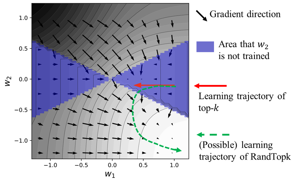
Figure 2: The loss surface, gradient field, and learning trajectory of the toy example.

Better convergence.

One concern about top-$k$ sparsification is that the model may be stuck at local minimums since those small neurons are not trained. RandTopk overcomes this problem naturally since its randomness, which makes small neurons get opportunities to be trained. Hence, the model will converge faster and to a better minimum.

To better illustrate this, we give the following toy example: Assume that we are learning the concept

$$f:(x_{1},x_{2})\rightarrow\text{Sign}(x_{1}-x_{2}),$$ (8)

with a simple split logistic model

$$\small\begin{split}&M_{h}:(x_{1},x_{2})\rightarrow(o_{1},o_{2})=(w_{1}x_{1},w_{2}x_{2}),\\ &M_{t}:(o_{1},o_{2})\rightarrow\text{Tanh}(o_{1}+o_{2}).\end{split}$$ (9)

The initial weights of the model are $w_{1}=1,w_{2}=-0.1$, and two samples are provided: $\mathbf{x}_{1}=(1,0),y_{1}=1$ and $\mathbf{x}_{2}=(0.5,1),y_{2}=-1$. It is obvious that if using top-$k$, $w_{1}=+\infty,w_{2}=-\infty$ are the optimal weights. However, the optimal weights can never be achieved since $o_{2}$ is always masked by top-$k$ sparsification, and $w_{2}$ is never trained. To make it clearer, we plot the loss surface and the gradient field of this example in Figure 2, and we fill the area where $w_{2}$ cannot be trained with blue. We can see that because of the non-continuity of gradient introduced by top-$k$, there is a bad local minimum in the blue area, and our training (red arrow) ends up there. Adding randomness to top-$k$, i.e., give non-top-$k$ neurons a chance to be selected, the problem can be solved instantly since $w_{2}$ will also be trained.

Better generalization.

As discussed above in Section 4.1, top-$k$ sparsification generalizes better since it has a larger feature space (under the same compression ratio) brought by total $d\choose k$ hyperspheres. However, training with top-$k$ sparsification cannot fully exploit the larger feature space, since the neurons are unevenly selected. Some neurons are constantly being selected with different input samples, while some are rarely selected. Those rarely selected neurons usually remain small for most input samples and are also rarely selected and trained throughout the training process. Consequently, the model cannot fully exploit the $d\choose k$ hyperspheres brought by top-$k$. For example, if there are $d^{\prime}$ neurons that never become top-$k$, then the feature space is reduced to ${{d-d^{\prime}}\choose k}<{d\choose k}$ hyperspheres. The margins between different classes are also smaller. RandTopk overcomes this problem since the small neurons are also selected. If some small neurons have the potential to become top-$k$ (w.r.t. certain input examples), RandTopk can provide them a chance to be large. Thus, the model can explore a larger space in those hyperspheres, and the margin will be larger, finally leading to a better generalization.

Task	Comp.	RandTopk	Topk	Size reduction	Quantization	L1 regularization
CIFAR-100 67.20 (0.71)	High	65.25 (0.54) / 2.86	62.23 (0.55) / 2.86	55.52 (0.69) / 3.13	-	-
	Medium	65.83 (0.56) / 5.71	61.56 (1.26) / 5.71	60.43 (0.33) / 6.25	53.56 (0.52) / 6.25	62.11 (0.56) / 8.41 (0.49)
	Low	65.98 (0.21) / 12.38	62.11 (0.71) / 12.38	62.93 (0.57) / 12.5	66.01 (0.23) / 12.5	63.87 (0.36) / 19.5 (2.25)
YooChoose 63.57 (0.57)	High	60.29 (0.05) / 0.85	60.28 (0.41) / 0.85	50.71 (1.51) / 1.00	-	-
	Medium	64.55 (0.16) / 1.71	63.81 (0.36) / 1.71	62.20 (0.50) / 2.00	-	-
	Low	66.88 (0.13) / 3.84	66.12 (0.44) / 3.84	66.12 (0.09) / 4.00	64.69 (0.21) / 3.13	61.48 (5.28) / 3.01 (1.12)
DBPedia 93.11 (0.13)	High+	84.88 (0.47) / 0.44	83.04 (0.45) / 0.44	64.80 (1.09) / 0.50	-	-
	High	88.01 (0.23) / 0.88	85.49 (0.35) / 0.88	78.57 (0.53) / 1.00	-	81.35 (0.68) / 1.08 (0.02)
	Medium	90.50 (0.11) / 1.97	87.74 (0.35) / 1.97	86.42 (0.26) / 2.00	-	87.88 (0.17) / 0.93 (0.01)
	Low	91.59 (0.50) / 3.06	90.05 (0.14) / 3.06	88.38 (0.10) / 3.00	91.20 (0.20) / 6.25	93.11 (0.05) / 5.31 (0.24)
TinyImagenet 53.11 (0.18)	High	50.83 (0.81) / 0.21	48.36 (0.09) / 0.21	35.46 (0.98) / 0.23	-	-
	Medium	51.75 (0.04) / 0.42	47.24 (0.09) / 0.42	45.66 (0.29) / 0.47	-	-
	Low	51.16 (0.14) / 0.94	45.50 (0.19) / 0.94	48.87 (0.14) / 0.14	-	-
TinyImagenet-p 75.18 (0.29)	High	71.09 (0.14) / 0.21	70.86 (0.07) / 0.21	59.23 (0.83) / 0.23	-	-
	Medium	72.15 (0.15) / 0.42	71.19 (0.54) / 0.42	66.52 (0.25) / 0.47	-	-
	Low	73.83 (0.20) / 0.94	72.52 (0.69) / 0.94	68.67 (0.16) / 0.94	-	67.82 (1.15) / 1.24 (0.04)

Table 3: Accuracy and Compressed size, in “Accuracy (standard deviation)/Compressed size (standard deviation, if not zero)” format. We assume the original communication size (non-compression case) to be 100. The accuracy of vanilla split training is under the dataset name. The best result is marked in bold, and the second-best result is underlined. The methods that fail to converge or are infeasible under the given compression level are omitted.

4.3 Discussion on Privacy

RandTopk has better input privacy than vanilla split learning since sparsification is performed on the bottom model output. This is because a large portion of the elements in the bottom model output are zeroed out, it contains less information than the original non-sparsified output, which has also been demonstrated by previous studies Zhu and Han (2020); Fu et al. (2022). We also provide the results on input reconstruction result in Appendix B. However, as split learning is vulnerable to label inference attacks Fu et al. (2022), RandTopk cannot preserve more label privacy. Hence, it is suitable for scenarios where the number of classes is large such that it is impossible for label inference attacks. For example, a face recognition model with thousands of different faces on user devices, or a recommendation model running on the user’s browser.

5 Experiments

5.1 Settings

Dataset	#Classes	Dim. of last layer
CIFAR-100	100	128
YooChoose	18,153	300
DBPedia	219	600
Tiny-Imagenet	200	1,280

Table 4: Dataset details.

We perform the experiments of different compression methods on four datasets, i.e., CIFAR-100 Krizhevsky et al. (2009), YooChoose Ben-Shimon et al. (2015), DBPedia Auer et al. (2007), and Tiny-Imagenet Le and Yang (2015), using Resnet-20 He et al. (2016), GRU4Rec Hidasi et al. (2016), TextCNN Kim (2014), and EfficientNet-b0 Tan and Le (2019), respectively. For CIFAR-100 and Tiny-Imagenet, data augmentation including random cropping and flipping is used. For YooChoose, we only use the latest 1/64 subset and apply the same data preprocessing as in Hidasi et al. (2016) while the loss function is changed to cross-entropy. The size of GRU layer is set to 300. For TextCNN, we set kernel sizes to [3,4,5] and use the Glove word embeddings  Pennington et al. (2014) as initialization. For Tiny-Imagenet, we train the model either from scratch (no suffix) or starting with pre-trained weights (marked by the suffix “-p”). The details of the datasets are provided in Table 4.

We split all the models by their last layer, and apply different compression methods with different compression ratios. All experiments are repeated 5 times, and the standard deviation is reported on the results. We report the results on accuracy vs. compression at the inference phase, convergence speed during training, in terms of epochs and communication size, and further analysis on the RandTopk corresponding to our theoretic claims in Section 4.2. Due to space limits, full experiment results, input reconstruction attacks, and analysis on the randomness coefficient $\alpha$ are placed in Appendix A, B, C, respectively.

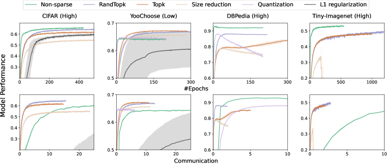
Figure 3: Convergence speed of different methods under certain compression levels. Compressed rates can be found in Table 3. Top row: accuracy vs. #epochs. Bottom row: Accuracy vs. communication (total size of the message transferred, vanilla split learning in one epoch = 1). Methods that are not applicable/fail to converge under the given compression level are omitted.

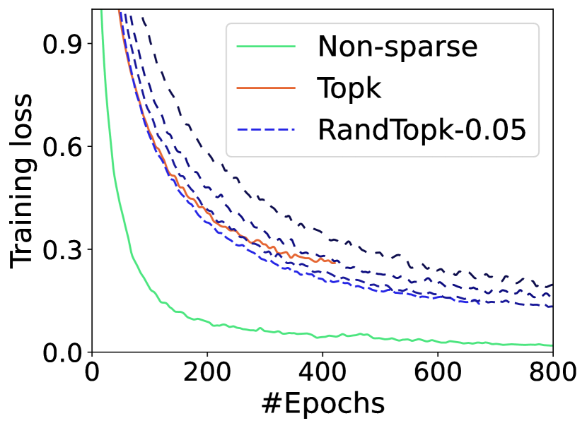
(a) Loss on the training set.

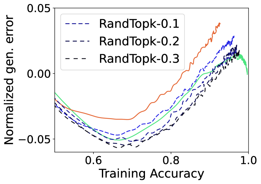
(b) Generalization error.

Figure 4: Training loss and generalization error on CIFAR-100. The compressed size is 2.86%.

5.2 Compressed Size vs. Performance

We report the test accuracy (hit ratio@20 for YooChoose) and corresponding compressed size for inference on different tasks and compression levels in Table 3. Each experiment has been repeated 3 times for TinyImagenet and 5 times for other tasks for more precise results. We set $\alpha$ to $0.1$ for all tasks except for YooChoose, where $\alpha=0.05$.

We can see that RandTopk achieves the best performance in almost all tasks and all compression levels, and are usually significantly better than the second-best method. Moreover, RandTopk’s performance is often very near to the non-sparse case (vanilla SL) even with a high compression ratio. RandTopk surpasses the non-compression case in the YooChoose task, which we think is caused by its regularization effect.

We also notice that quantization and L1 regularization are not applicable under many compression levels. For quantization, it can only achieve a maximum compression ratio of 32, and 1-bit quantization usually fails to converge. L1 regularization, on the other side, makes training difficult and usually fails to converge.

5.3 Convergence Speed

Although our main purpose is to reduce communication at the inference phase, we also report the convergence speed during training in Figure 3. The convergence speed is measured in two terms: the number of epochs and the communication size.

We can see that non-sparse (vanilla SL) training takes the least epochs to converge, while RandTopk and other compression methods converge slower, but the difference is not large to the magnitude level. As for the overall communication to converge or reach a certain accuracy level, almost all compression methods outperforms the non-sparse training. RandTopk performs best in terms of convergence speed and performance among all other methods.

5.4 Further Analysis on RandTopk

To verify our theoretical analysis in Section 4.2, we provide the results on convergence speed, generalization error, and the distribution of top-$k$ neurons during training using CIFAR-100, to demonstrate the advantage of RandTopk.

Faster convergence.

We plot the loss curve of top-$k$ and RandTopk with different $\alpha$ in Figure 44(a). We can see that at first top-$k$ sparsification converges faster, then gradually slows. With a small $\alpha$, RandTopk converges faster and reaches a smaller loss value. When $\alpha$ becomes larger, the convergence at the beginning is slower, however, later it will exceed top-$k$. The result verifies our argument that RandTopk can help avoid local minimums that top-$k$ may get stuck at.

Better generalization.

We report the generalization error in Figure 44(b). We notice that for all methods, the generalization error can be approximated by $0.5\times\text{train acc.}-0.2$. Hence, the y-axis is set to be the difference between generalization error and this value for better illustration. We can see that when the train set accuracy is the same, RandTopk has a significantly lower generalization error than top-$k$, and larger $\alpha$ further decreases the generalization error. This supports our argument that RandTopk generalizes better.

Distribution of top-$k$ neurons.

We report the histogram of the times a neuron become top-$k$. More specifically, after model training is finished, we iterate through the train set and record the top-$k$ neurons for each input example. Notice that we perform this experiment on the inference phase, hence RandTopk also behaves deterministically like top-$k$. As we can see in Figure 5, if trained with top-$k$ sparsification, some neurons will become top-$k$ neurons very often, while some rarely become top-$k$. More specifically, some neurons become top-$k$ for less than 500 times, while some neurons become top-$k$ for more than 3,500 times. Using RandTopk, the distribution is more balanced, e.g., no neuron becomes top-$k$ more than 3,000 times or less than 250 times. Larger $\alpha$ makes the distribution more balanced. The results verify our argument that RandTopk can make use of the expanded feature space better.

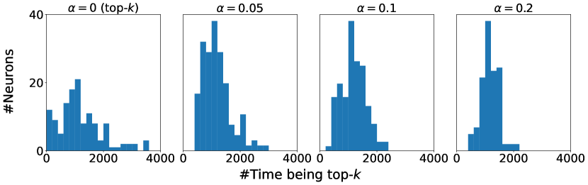
Figure 5: Distribution of top-$k$ neurons during inference.

6 Conclusion

In this paper, we investigate the use of different compression methods in split learning. By the analysis of the size reduction method and top-$k$ sparsification, we further propose randomized top-$k$ sparsification, which strengthens top-$k$’s advantage on generalization ability while avoiding its disadvantage on convergence. Experiments on multiple datasets and different kinds of models show that randomized top-$k$ is superior to other sparsification methods in terms of model performance and compression ratio. However, there are still some issues worth studying in the future. On the one hand, the label privacy remains to be a problem. Moreover, further research on compression for split learning is needed, for example, combining quantization and sparsification can be promising.

Appendix A Detailed results on accuracy and compressed size

We provide all results on accuracy and compressed size of all four tasks, in Table 5, 6, 7 and 8. The coefficient of L1-regularization and RandTopk ($\alpha$) is marked. For example, L1-0.001 means the regularization coefficient is 0.001, and RandTopk-0.1 means RandTopk with $\alpha=0.1$.

Appendix B Input privacy

We also simulate the input inversion attack (i.e., inferring input from the bottom model output) on CIFAR-100, to show the privacy-preserving power of RandTopk. We compared the non-sparse case (vanilla SL), with top-$k$ and RandTopk ($\alpha\in\{0.05,0.1,0.2\}$) sparsification of compressed size $2.86\%$, i.e., 3 out of 128 elements are preserved. We train a generator network (made of Conv and DeConv layers) from the train set, whose input is the bottom model output and label is the original input image. After training for 1,000 epochs, we use the test set to conduct the inversion attack. The reconstruction error (squared loss) is reported in Figure 7. The original images and the generated images are shown in Figure 6. We can see that using RandTopk, whatever $\alpha$ is, the reconstruction error is larger than top-$k$, and also much larger than the non-sparse case. The reconstructed images are also very blurry and contain little information about the original input.

Appendix C Impact of $\alpha$

As described in Section 4.2, $\alpha$ is used to control the randomness of RandTopk, and will potentially influence the model performance. Hence, we report the results of using different $\alpha$ on the CIFAR-100 and YooChoose datasets.

We can see that, for the CIFAR-100 task, all choices of $\alpha\in\{0.05,0.1,0.2,0.3\}$ perform significantly better than the top-$k$ (i.e., $\alpha=0$), while $\alpha=0.1$ achieves the best performance. As for the YooChoose task, the best choice of $\alpha$ is around $0.05\sim 0.1$. Larger $\alpha$ leads to a significant performance drop, making it even worse than top-$k$. Generally, too large $\alpha$ will introduce too much noise and damage the model performance, while $\alpha$ around $0.05\sim 0.1$ achieves good performance.

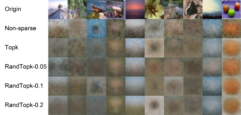
Figure 6: Inversion attack on CIFAR-100

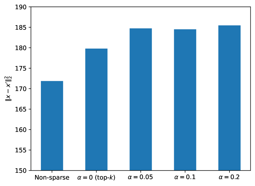
Figure 7: Reconstruction error of RandTopk on CIFAR-100

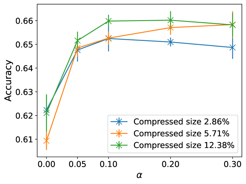
(a) CIFAR.

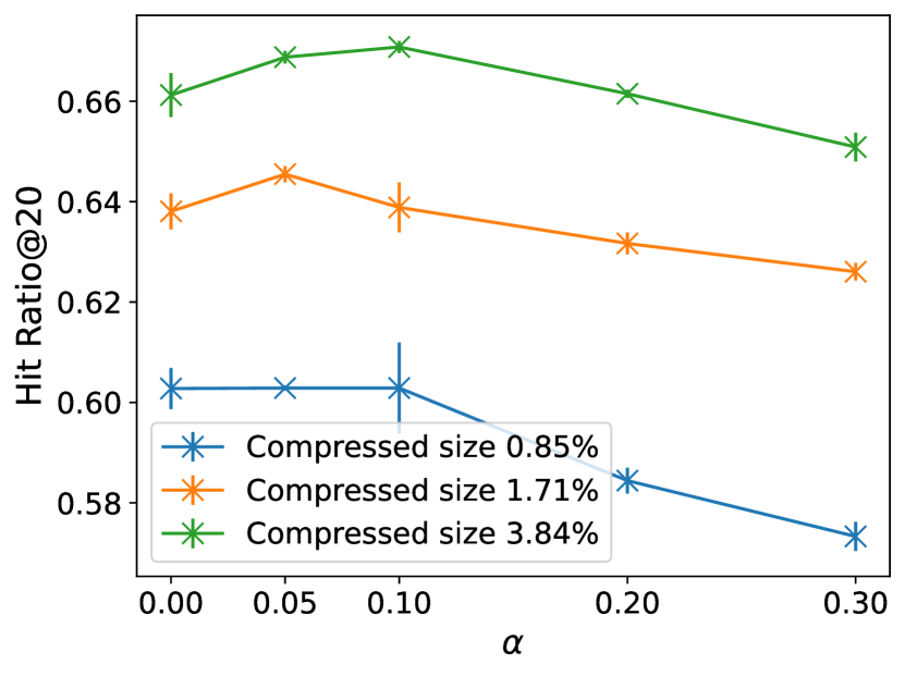
(b) YooChoose.

Figure 8: Test accuracy on different $\alpha$.

Table 5: Test accuracy and compression ratio on CIFAR-100.

Method	Compressed size (%)	Test accuracy
No compression	100	67.20 (0.71)
Topk	2.86	62.23 (0.55)
RandTopk-0.05	2.86	64.76 (0.49)
RandTopk-0.1	2.86	65.25 (0.54)
RandTopk-0.2	2.86	65.10 (0.19)
RandTopk-0.3	2.86	64.87 (0.48)
Size reduction	3.13	55.52 (0.69)
L1-0.001	5.45 (0.29)	60.96 (0.67)
Topk	5.71	61.56 (1.26)
RandTopk-0.05	5.71	64.84 (0.37)
RandTopk-0.1	5.71	65.26 (0.28)
RandTopk-0.2	5.71	65.71 (0.31)
RandTopk-0.3	5.71	65.83 (0.56)
Size reduction	6.25	60.43 (0.33)
Quantization-2bit	6.25	53.56 (0.52)
L1-0.0005	8.41 (0.49)	62.11 (0.56)
Topk	12.38	62.11 (0.79)
RandTopk-0.05	12.38	65.16 (0.37)
RandTopk-0.1	12.38	65.98 (0.27)
RandTopk-0.2	12.38	66.02 (0.38)
RandTopk-0.3	12.38	65.98 (0.27)
Size reduction	12.5	62.93 (0.57)
Quantization-4bit	12.5	66.01 (0.23)
L1-0.0002	19.5 (2.25)	63.87 (0.36)

Table 6: Test accuracy and compression ratio on YooChoose.

Method	Compressed size (%)	Test hr@20
No compression	100	63.57 (0.57)
Topk	0.85	60.28 (0.41)
RandTopk-0.05	0.85	60.29 (0.05)
RandTopk-0.1	0.85	60.29 (0.91)
RandTopk-0.2	0.85	58.44 (0.25)
RandTopk-0.3	0.85	57.33 (0.29)
Size reduction	1.00	50.73 (1.51)
Topk	1.71	63.81 (0.36)
RandTopk-0.05	1.71	64.55 (0.16)
RandTopk-0.1	1.71	63.89 (0.50)
RandTopk-0.2	1.71	63.17 (0.22)
RandTopk-0.3	1.71	62.60 (0.18)
Size reduction	2.00	62.20 (0.50)
L1-0.002	3.01 (1.12)	61.48 (5.28)
Quantization-1bit	3.13	64.69 (0.21)
Topk	3.84	66.12 (0.44)
RandTopk-0.05	3.84	66.88 (0.13)
RandTopk-0.1	3.84	67.08 (0.12)
RandTopk-0.2	3.84	66.15 (0.08)
RandTopk-0.3	3.84	65.09 (0.29)
Size reduction	4.00	66.12 (0.09)

Table 7: Test accuracy and compression ratio on DBPedia.

Method	Compressed size (%)	Test accuracy
No Compression	100	93.11 (0.13)
Topk	0.44	83.04 (0.45)
RandTopk-0.1	0.44	84.88 (0.47)
Size reduction	0.50	64.80 (1.09)
Topk	0.88	85.49 (0.35)
RandTopk-0.1	0.88	88.01 (0.23)
L1-0.002	0.93 (0.01)	78.68 (0.83)
Size reduction	1.00	78.57 (0.53)
L1-0.001	1.08 (0.02)	81.35 (0.68)
L1-0.0005	1.45 (0.02)	87.88 (0.17)
Topk	1.97	87.74 (0.35)
RandTopk-0.1	1.97	90.50 (0.11)
Size reduction	2.00	86.42 (0.26)
Size reduction	3.00	88.38 (0.10)
Topk	3.06	90.05 (0.14)
RandTopk-0.1	3.06	91.59 (0.50)
L1-0.0002	3.08 (0.09)	92.16 (0.10)
L1-0.0001	5.31 (0.24)	93.11 (0.05)
Quantization-2bit	6.25	91.20 (0.20)

Table 8: Test accuracy and compression ratio on Tiny-Imagenet.

Use ImageNet pre-trained weights
Method	Compressed size (%)	Test accuracy
No compression	100	75.18 (0.29)
TopK	0.21	70.86 (0.07)
RandTopk-0.1	0.21	71.09 (0.14)
Size reduction	0.23	59.23 (0.83)
TopK	0.42	71.79 (0.54)
RandTopk-0.1	0.42	72.15 (0.15)
Size reduction	0.47	66.52 (0.25)
TopK	0.94	72.52 (0.69)
RandTopk-0.1	0.94	73.83 (0.20)
Size reduction	0.94	68.67 (0.16)
L1-0.0001	1.24 (0.04)	67.82 (1.15)
Train from scratch
Method	Compressed size (%)	Test accuracy
No compression	100	53.11 (0.18)
TopK	0.21	48.36 (0.09)
RandTopk-0.1	0.21	50.83 (0.81)
Size reduction	0.23	35.46 (0.98)
TopK	0.42	47.24 (0.09)
RandTopk-0.1	0.42	51.75 (0.04)
Size reduction	0.47	45.66 (0.29)
TopK	0.94	45.50 (0.19)
RandTopk-0.1	0.94	51.16 (0.14)
Size reduction	0.94	48.87 (0.14)

Appendix D Derivation of Equation 6

The $k$-dimensional hypersphere $\|\mathbf{w}\|_{2}=1$ has a volume of $2\pi^{k/2}/\Gamma{(k/2)}$, and each $(k-1)$-dimensional ball $B_{i}$ has a volume of $2\pi^{(k-1)/2}/\Gamma{[(k+1)/2]}$. Hence, if there are $n$ balls, the upper bound of minimum center distance (the margin between two classes’ weights) $d_{W}$ shall satisfy

$$n\cdot\pi^{(k-1)/2}/\Gamma{\left(\dfrac{k+1}{2}\right)}(d_{W}/2)^{k-1}\approx 2\pi^{k/2}/\Gamma{\left(\dfrac{k}{2}\right)},$$ (10)

then we have

$$\left(\dfrac{d_{W}}{2}\right)^{k-1}\approx\dfrac{2{\sqrt{\pi}}}{n}\cdot\dfrac{\Gamma{[(k+1)/2]}}{\Gamma{(k/2)}}.$$ (11)

Notice the fact that $\Gamma(x+1/2)/\Gamma(x)\approx\sqrt{x}$, we can further obtain

$$d_{W}\approx 2\cdot\left(\dfrac{2}{n}\sqrt{\dfrac{k\pi}{2}}\right)^{1/(k-1)}.$$ (12)

In the above analysis, $d_{W}$ is the estimated maximum distance for size reduction, whose feature space is a $k$-dimensional hypersphere. On the other side, for top-$k$ sparsification, the feature space contains ${d\choose k}$ hyperspheres since there are total ${d\choose k}$ choices to select $k$ dimensions out of $d$ dimensions. Also, considering the extra communication for indices, we have to reduce the preserved non-zero elements of top-$k$ from $k$ to $\alpha k$, where $\alpha\in(1/2,1)$.

Hence, center distance $d_{W}^{\prime}$ is changed to

$$d_{W}^{\prime}\approx{d\choose\alpha k}\cdot 2\cdot\left(\dfrac{2}{n}\sqrt{\dfrac{\alpha k\pi}{2}}\right)^{1/(\alpha k-1)}.$$ (13)

Combining (12) and $\eqref{eq:dist-topk}$, we have:

$$\begin{split}\dfrac{d_{W}^{\prime}}{d_{W}}&\approx{d\choose\alpha k}\dfrac{(2/n\sqrt{\alpha k\pi/2})^{1/(\alpha k-1)}}{(2/n\sqrt{k\pi/2})^{1/(k-1)}}\\ &={d\choose\alpha k}\left(\dfrac{2}{n}\sqrt{\dfrac{\alpha k\pi}{2}}\right)^{1/(\alpha k-1)}\cdot\alpha^{\dfrac{1}{2}\left(\dfrac{1}{\alpha k-1}-\dfrac{1}{k-1}\right)}.\end{split}$$ (14)

Notice that for if $x,y\in(0,1)$, then $x^{y}>x$ (immediately from $y\ln x>\ln x$). Since $1/(\alpha k-1),1/(\alpha k-1)-1/(k-1)\in(0,1)$, as long as $2/n\sqrt{\alpha k\pi/2}<1$, we have

$$\left(\dfrac{2}{n}\sqrt{\dfrac{\alpha k\pi}{2}}\right)^{1/(\alpha k-1)-1/(k-1)}\geq\dfrac{2}{n}\sqrt{\dfrac{\alpha k\pi}{2}},$$ (15)

and also we have $\alpha^{1/(2(k-1)}\geq\alpha$. Plug these into (14), we obtain

$$\dfrac{d_{W}^{\prime}}{d_{W}}\gtrsim{d\choose\alpha k}\dfrac{2}{n}\sqrt{\dfrac{\alpha k\pi}{2}}\alpha={d\choose\alpha k}\cdot\dfrac{\sqrt{2\alpha^{3}k\pi}}{n},$$ (16)

which is Equation 6, as we use $d_{W}$ to denote $d_{W}^{\text{(size reduction)}}$ and $d_{W}^{\prime}$ to denote $d^{\text{(top-$k$)}}$.

References

- Aji and Heafield [2017] Alham Fikri Aji and Kenneth Heafield. Sparse communication for distributed gradient descent. In Proceedings of the 2017 Conference on Empirical Methods in Natural Language Processing, EMNLP 2017, Copenhagen, Denmark, September 9-11, 2017, pages 440–445. Association for Computational Linguistics, 2017.
- Auer et al. [2007] Sören Auer, Christian Bizer, Georgi Kobilarov, Jens Lehmann, Richard Cyganiak, and Zachary G. Ives. Dbpedia: A nucleus for a web of open data. In The Semantic Web, 6th International Semantic Web Conference, 2nd Asian Semantic Web Conference, ISWC 2007 + ASWC 2007, volume 4825 of Lecture Notes in Computer Science, pages 722–735. Springer, 2007.
- Ayad et al. [2021] Ahmad Ayad, Melvin Renner, and Anke Schmeink. Improving the communication and computation efficiency of split learning for iot applications. In IEEE Global Communications Conference, GLOBECOM 2021, Madrid, Spain, December 7-11, 2021, pages 1–6. IEEE, 2021.
- Ben-Shimon et al. [2015] David Ben-Shimon, Alexander Tsikinovsky, Michael Friedmann, Bracha Shapira, Lior Rokach, and Johannes Hoerle. Recsys challenge 2015 and the yoochoose dataset. In Proceedings of the 9th ACM Conference on Recommender Systems, pages 357–358, 2015.
- Castiglia et al. [2022] Timothy J. Castiglia, Anirban Das, Shiqiang Wang, and Stacy Patterson. Compressed-vfl: Communication-efficient learning with vertically partitioned data. In International Conference on Machine Learning, ICML 2022, volume 162 of Proceedings of Machine Learning Research, pages 2738–2766. PMLR, 2022.
- Chandar et al. [2021] Srikanth Chandar, Pravin Chandran, Raghavendra Bhat, and Avinash Chakravarthi. Communication optimization in large scale federated learning using autoencoder compressed weight updates. CoRR, abs/2108.05670, 2021.
- Chen et al. [2021a] Chaochao Chen, Jun Zhou, Li Wang, Xibin Wu, Wenjing Fang, Jin Tan, Lei Wang, Alex X. Liu, Hao Wang, and Cheng Hong. When homomorphic encryption marries secret sharing: Secure large-scale sparse logistic regression and applications in risk control. In Feida Zhu, Beng Chin Ooi, and Chunyan Miao, editors, KDD ’21: The 27th ACM SIGKDD Conference on Knowledge Discovery and Data Mining, pages 2652–2662. ACM, 2021.
- Chen et al. [2021b] Xing Chen, Jingtao Li, and Chaitali Chakrabarti. Communication and computation reduction for split learning using asynchronous training. In IEEE Workshop on Signal Processing Systems, SiPS 2021, pages 76–81. IEEE, 2021.
- Chen et al. [2022] Chaochao Chen, Jun Zhou, Longfei Zheng, Huiwen Wu, Lingjuan Lyu, Jia Wu, Bingzhe Wu, Ziqi Liu, Li Wang, and Xiaolin Zheng. Vertically federated graph neural network for privacy-preserving node classification. In Luc De Raedt, editor, Proceedings of the Thirty-First International Joint Conference on Artificial Intelligence, IJCAI 2022, pages 1959–1965. ijcai.org, 2022.
- Fu et al. [2022] Chong Fu, Xuhong Zhang, Shouling Ji, Jinyin Chen, Jingzheng Wu, Shanqing Guo, Jun Zhou, Alex X. Liu, and Ting Wang. Label inference attacks against vertical federated learning. In 31st USENIX Security Symposium (USENIX Security 22), Boston, MA, August 2022. USENIX Association.
- Gholami et al. [2021] Amir Gholami, Sehoon Kim, Zhen Dong, Zhewei Yao, Michael W. Mahoney, and Kurt Keutzer. A survey of quantization methods for efficient neural network inference. CoRR, abs/2103.13630, 2021.
- Gouk et al. [2021] Henry Gouk, Eibe Frank, Bernhard Pfahringer, and Michael J. Cree. Regularisation of neural networks by enforcing lipschitz continuity. Mach. Learn., 110(2):393–416, 2021.
- He et al. [2016] Kaiming He, Xiangyu Zhang, Shaoqing Ren, and Jian Sun. Deep residual learning for image recognition. In 2016 IEEE Conference on Computer Vision and Pattern Recognition, CVPR 2016, pages 770–778. IEEE Computer Society, 2016.
- Hidasi et al. [2016] Balázs Hidasi, Alexandros Karatzoglou, Linas Baltrunas, and Domonkos Tikk. Session-based recommendations with recurrent neural networks. In 4th International Conference on Learning Representations, ICLR 2016, 2016.
- Jacob et al. [2018] Benoit Jacob, Skirmantas Kligys, Bo Chen, Menglong Zhu, Matthew Tang, Andrew G. Howard, Hartwig Adam, and Dmitry Kalenichenko. Quantization and training of neural networks for efficient integer-arithmetic-only inference. In 2018 IEEE Conference on Computer Vision and Pattern Recognition, CVPR 2018, pages 2704–2713. Computer Vision Foundation / IEEE Computer Society, 2018.
- Jin et al. [2022] Jiayin Jin, Jiaxiang Ren, Yang Zhou, Lingjuan Lyu, Ji Liu, and Dejing Dou. Accelerated federated learning with decoupled adaptive optimization. In International Conference on Machine Learning, pages 10298–10322. PMLR, 2022.
- Karimireddy et al. [2020] Sai Praneeth Karimireddy, Satyen Kale, Mehryar Mohri, Sashank J. Reddi, Sebastian U. Stich, and Ananda Theertha Suresh. SCAFFOLD: stochastic controlled averaging for federated learning. In Proceedings of the 37th International Conference on Machine Learning, ICML 2020, 13-18 July 2020, Virtual Event, volume 119 of Proceedings of Machine Learning Research, pages 5132–5143. PMLR, 2020.
- Kim [2014] Yoon Kim. Convolutional neural networks for sentence classification. In Proceedings of the 2014 Conference on Empirical Methods in Natural Language Processing, EMNLP 2014, pages 1746–1751. ACL, 2014.
- Krizhevsky et al. [2009] Alex Krizhevsky, Geoffrey Hinton, et al. Learning multiple layers of features from tiny images. Master’s thesis, Department of Computer Science, University of Toronto, 2009.
- Le and Yang [2015] Ya Le and Xuan Yang. Tiny imagenet visual recognition challenge. CS 231N, 7(7):3, 2015.
- Li et al. [2020] Tian Li, Anit Kumar Sahu, Ameet Talwalkar, and Virginia Smith. Federated learning: Challenges, methods, and future directions. IEEE Signal Processing Magazine, 37(3):50–60, 2020.
- McMahan et al. [2017] Brendan McMahan, Eider Moore, Daniel Ramage, Seth Hampson, and Blaise Agüera y Arcas. Communication-efficient learning of deep networks from decentralized data. In Proceedings of the 20th International Conference on Artificial Intelligence and Statistics, AISTATS 2017, volume 54 of Proceedings of Machine Learning Research, pages 1273–1282. PMLR, 2017.
- Mohassel and Rindal [2018] Payman Mohassel and Peter Rindal. Aby: A mixed protocol framework for machine learning. In Proceedings of the 2018 ACM SIGSAC Conference on Computer and Communications Security, CCS 2018, pages 35–52. ACM, 2018.
- Neyshabur et al. [2015] Behnam Neyshabur, Ryota Tomioka, and Nathan Srebro. Norm-based capacity control in neural networks. In Proceedings of The 28th Conference on Learning Theory, COLT 2015, volume 40 of JMLR Workshop and Conference Proceedings, pages 1376–1401. JMLR.org, 2015.
- Neyshabur et al. [2017] Behnam Neyshabur, Srinadh Bhojanapalli, David McAllester, and Nati Srebro. Exploring generalization in deep learning. In Advances in Neural Information Processing Systems 30: NeurIPS 2017, pages 5947–5956, 2017.
- Pennington et al. [2014] Jeffrey Pennington, Richard Socher, and Christopher D Manning. Glove: Global vectors for word representation. In Proceedings of the 2014 conference on empirical methods in natural language processing (EMNLP), pages 1532–1543, 2014.
- Sattler et al. [2019a] Felix Sattler, Simon Wiedemann, Klaus-Robert Müller, and Wojciech Samek. Robust and communication-efficient federated learning from non-iid data. CoRR, abs/1903.02891, 2019.
- Sattler et al. [2019b] Felix Sattler, Simon Wiedemann, Klaus-Robert Müller, and Wojciech Samek. Sparse binary compression: Towards distributed deep learning with minimal communication. In International Joint Conference on Neural Networks, IJCNN 2019 Budapest, Hungary, July 14-19, 2019, pages 1–8. IEEE, 2019.
- Stich et al. [2018] Sebastian U. Stich, Jean-Baptiste Cordonnier, and Martin Jaggi. Sparsified SGD with memory. In Advances in Neural Information Processing Systems 31: NeurIPS 2018, pages 4452–4463, 2018.
- Tan and Le [2019] Mingxing Tan and Quoc V. Le. Efficientnet: Rethinking model scaling for convolutional neural networks. In Proceedings of the 36th International Conference on Machine Learning, ICML 2019, volume 97 of Proceedings of Machine Learning Research, pages 6105–6114. PMLR, 2019.
- Tibshirani [1996] Robert Tibshirani. Regression shrinkage and selection via the lasso. Journal of the Royal Statistical Society: Series B (Methodological), 58(1):267–288, 1996.
- Vepakomma et al. [2018] Praneeth Vepakomma, Otkrist Gupta, Tristan Swedish, and Ramesh Raskar. Split learning for health: Distributed deep learning without sharing raw patient data. arXiv preprint arXiv:1812.00564, 2018.
- Vogels et al. [2019] Thijs Vogels, Sai Praneeth Karimireddy, and Martin Jaggi. Powersgd: Practical low-rank gradient compression for distributed optimization. In Advances in Neural Information Processing Systems 32: NeurIPS 2019, pages 14236–14245, 2019.
- Wagh et al. [2019] Sameer Wagh, Divya Gupta, and Nishanth Chandran. Securenn: 3-party secure computation for neural network training. Proc. Priv. Enhancing Technol., 2019(3):26–49, 2019.
- Wang et al. [2018] Hongyi Wang, Scott Sievert, Shengchao Liu, Zachary B. Charles, Dimitris S. Papailiopoulos, and Stephen J. Wright. ATOMO: communication-efficient learning via atomic sparsification. In Advances in Neural Information Processing Systems 31: NeurIPS 2018, pages 9872–9883, 2018.
- Wang et al. [2020a] Hongyi Wang, Mikhail Yurochkin, Yuekai Sun, Dimitris S. Papailiopoulos, and Yasaman Khazaeni. Federated learning with matched averaging. In 8th International Conference on Learning Representations, ICLR 2020, Addis Ababa, Ethiopia, April 26-30, 2020. OpenReview.net, 2020.
- Wang et al. [2020b] Jianyu Wang, Qinghua Liu, Hao Liang, Gauri Joshi, and H. Vincent Poor. Tackling the objective inconsistency problem in heterogeneous federated optimization. In Advances in Neural Information Processing Systems 33: NeurIPS 2020, 2020.
- Wen et al. [2017] Wei Wen, Cong Xu, Feng Yan, Chunpeng Wu, Yandan Wang, Yiran Chen, and Hai Li. Terngrad: Ternary gradients to reduce communication in distributed deep learning. In Advances in Neural Information Processing Systems 30: NeurIPS 2017, pages 1509–1519, 2017.
- Wright et al. [2008] John Wright, Allen Y Yang, Arvind Ganesh, S Shankar Sastry, and Yi Ma. Robust face recognition via sparse representation. IEEE transactions on pattern analysis and machine intelligence, 31(2):210–227, 2008.
- Yin et al. [2012] Jun Yin, Zhonghua Liu, Zhong Jin, and Wankou Yang. Kernel sparse representation based classification. Neurocomputing, 77(1):120–128, 2012.
- Zhu and Han [2020] Ligeng Zhu and Song Han. Deep leakage from gradients. In Federated Learning - Privacy and Incentive, volume 12500 of Lecture Notes in Computer Science, pages 17–31. Springer, 2020.