Geometric Graph Filters and Neural Networks:
Limit Properties and Discriminability Trade-offs
Abstract
This paper studies the relationship between a graph neural network (GNN) and a manifold neural network (MNN) when the graph is constructed from a set of points sampled from the manifold, thus encoding geometric information. We consider convolutional MNNs and GNNs where the manifold and the graph convolutions are respectively defined in terms of the Laplace-Beltrami operator and the graph Laplacian. Using the appropriate kernels, we analyze both dense and moderately sparse graphs. We prove non-asymptotic error bounds showing that convolutional filters and neural networks on these graphs converge to convolutional filters and neural networks on the continuous manifold. As a byproduct of this analysis, we observe an important trade-off between the discriminability of graph filters and their ability to approximate the desired behavior of manifold filters. We then discuss how this trade-off is ameliorated in neural networks due to the frequency mixing property of nonlinearities. We further derive a transferability corollary for geometric graphs sampled from the same manifold. We validate our results numerically on a navigation control problem and a point cloud classification task.
Index Terms:
Graph Neural Networks, Manifold Filters, Manifold Neural Networks, Convergence Analysis, DiscriminabilityI Introduction
Geometric data, or data supported in non-Euclidean domains, is the object of much interest in modern information processing. It arises in a number of applications, including protein function prediction [3, 4], robot path planning [5, 6], 3D shape analysis [7, 8, 9] and wireless resource allocation [10, 11]. Graph convolutional filters [12, 13] and graph neural networks (GNNs) [14, 15], along with manifold convolutional filters [16] and manifold neural networks (MNNs) [17, 18, 19], are the standard tools for invariant information processing on these domains when they are discrete and continuous respectively. The convolution operation is implemented through information diffusion over the geometric structure, thus enabling invariant and stable representations [20, 21, 22, 23] and feature sharing. The cascading neural network architecture interleaves convolutions and nonlinearities, further expanding the model’s expressiveness.
Although there is a clear parallel between graphs and manifolds—the former can be seen as discretizations of the latter—, manifolds are infinite-dimensional continuous latent spaces which can only be accessed by discrete point sampling [7, 24, 25, 26]. In general, we have access to a set of sampling points from the manifold, and build a graph model to approximate the underlying continuous manifold while attempting to retain the local and global geometric structure [27, 7, 11]. GNNs have been shown to do well at processing information over the manifold both experimentally and theoretically [25, 16, 28]. Of particular note, conditions that guarantee asymptotic convergence of graph filters and GNNs to manifold filters and MNNs are known [16].
Asymptotic convergence is a minimal guarantee that can be enriched with non-asymptotic approximation error bounds. These bounds are unknown and they are the focus of this paper. These non-asymptotic approximation error bounds relating graph filters and GNNs to manifold filters and MNNs are important because they inform the practical design on graphs of information processing architectures that we want to deploy on manifolds. In addition, explicit finite-sample error bounds often reveal details about the convergence regime (e.g., rates of convergence and discriminability trade-offs) that are not revealed by their asymptotic counterparts. For example, the non-asymptotic convergence analysis of GNNs on graphs sampled from a graphon (also referred to as a transferability analysis) gives a more precise characterization of the discriminability-convergence tradeoff that arises in these GNNs [29], which is not elucidated by the corresponding asymptotic convergence result [30].
Contributions. In this paper, we prove and analyze a non-asymptotic approximation error bound for GNNs on graphs sampled from manifold, thus closing the gap between GNNs and MNNs with an explicit numerical relationship. We start by importing the definition of the manifold filter as a convolutional operation where the diffusions are exponentials of the Laplace-Beltrami (LB) operator of the manifold [16]. Given a set of discrete sampling points from the manifold, we describe how to construct both dense and relatively sparse geometric graphs that approximate the underlying manifold in both the spatial and the spectral domains.
Next, we import the concept of Frequency Difference Threshold (FDT) filters (Definition 3) [17] to overcome the challenge of dimensionality associated with the infinite-dimensional spectrum of the LB operator. We show that manifold filters exhibit a trade-off between their discriminability and their ability to be approximated by graph filters, which can be observed in the approximation error bound of geometric graph filters in Theorems 1 and 2.
The same analysis is conducted for GNNs by incorporating nonlinearities (Theorem 3), but in GNNs we hypothesize that the trade-off is alleviated, i.e., that we can recover discriminability, through the addition of these nonlinear operations (Section V). In other words, geometric GNNs can be both discriminative and approximative of the underlying MNNs, which we verify empirically through numerical experiments (Section VI). Finally, we show how our approximation result can be extended, by a triangle inequality argument, to a transferability result for geometric GNNs transferred across geometric graphs of different sizes sampled from the same underlying manifold.
Related Works. GNNs have been thoroughly studied and discussed in a number of previous works [15, 31, 14]. Similarly, the convergence and transferability of neural networks on graphs have been studied in many works including [32, 21, 33, 29]. These works however see the graphs as samples from a graphon model. In our paper, we focus on the manifold as the limit model for large-scale graphs, which is more realistic than graphons as it can incorporate the underlying geometric information. Moreover, the manifold can also represent the limit of sparse or relatively sparse graphs. Very relevant to this paper, the spectral convergence of relatively sparse graphs sampled from manifolds has been studied at length in [34].
Manifold filters and manifold neural networks have been established and discussed in [16, 17, 18, 24] using different features and metrics. The integral of the heat diffusion process is employed in [16, 17] where it is shown that manifold convolutions are consistent with and can recover both the graph convolution and the time convolution. In [18], a local geodesic system capturing local anisotropic structures is used to define the manifold convolution. Taking a different approach, [24] defines a mixture Gaussian kernel over the spatial domain using patch operator that is constructed locally.
Among all these methods, the definition leveraging the heat diffusion process is the only one to build the connection between graph neural networks and manifold neural networks when the graphs are sampled from the manifold [16]. However, this paper does not provide an explicit convergence rate or approximation error bound between GNNs and MNNs. In [35], a convergence rate is given for GNNs approximating MNNs, but the result is restricted to input signals with a limited bandwidth. Moreover, the graphs constructed in [16] and [35] still need to be dense with a well-defined Gaussian kernel. In contrast, in this paper we extend the analysis of the convergence of GNNs by proving a non-asymptotic approximation error bound for geometric GNNs sampled from the MNNs where the geometric graphs are either dense or relatively sparse; and we eliminate the bandlimited signal assumption by importing frequency-dependent filters.
Organization. Section II introduces preliminary definitions of graph signal processing and graph neural networks along with manifold signal processing and manifold neural networks. Section III introduces the construction of the geometric graphs from the sampling points of the manifold and the convergence of the geometric graph Laplacians. We show the spectrum of the geometric graphs – both dense and relatively sparse – can approximate the spectrum of the LB operator of the underlying manifold with a bounded error. We then go on to study the approximation of the filtering on the geometric graphs which is further extended to the approximation of geometric GNNs to MNNs in Section IV. Section V discusses the implications of the results derived in Section IV. Section VI illustrates the results of Sections IV with numerical examples. Section VII concludes the paper. Proofs are deferred to the appendices and supplementary materials.
II Preliminary Definitions
We start by reviewing the basic architecture of graph neural networks and manifold neural networks.
II-A Graph Signal Processing and Graph Neural Networks
Let be an undirected graph with node set , and edge set . The edges in may be weighted, in which case the edge weights are assigned by a function . In this paper, we are interested in graph signals supported on the nodes. For , represents the value of the signal at node .
Graph shift. Operating on graph signals , we define the graph shift operator (GSO) . The GSO is any matrix satisfying if and only if or , e.g., the adjacency matrix , , or the graph Laplacian [13, 36]. The GSO is so called because, at each node , it has the effect of shifting or diffusing the signal values at ’s neighbors to , where signal values are aggregated. Explicitly, . In the case of an undirected graph, the GSO is symmetric and can therefore be decomposed as . The eigenvalues in the diagonal matrix are seen as graph frequencies, and the eigenvectors in are the corresponding graph oscillation modes.
Graph convolution. A graph convolution is defined based on the graph diffusion process with consecutive shifts. More formally, the graph convolutional filter [15, 13, 37] with coefficients is given by
| (1) |
Plugging the spectral decomposition of into (1), we see that in the spectral domain this filter can be represented as
| (2) |
Hence, the graph frequency response of the graph convolution is given by , which only depends on the weights and on the eigenvalues of .
Graph neural network. A graph neural network (GNN) is built by cascading layers that each consists of a bank of filters followed by a point-wise nonlinearity , . The th layer of a GNN produces signals , each called a feature, given by
| (3) |
for . At each layer , the number of input and output features are and respectively. The filter is as in (1) and maps the -th feature of layer to the -th feature of layer . For simplicity, we write the GNN consisting of layers like (3) as the map , where denotes a set of the graph filter coefficients at all layers.
II-B Manifold Signal Processing and Manifold Neural Networks
Let be a -dimensional embedded manifold in . For simplicity, in this paper whenever we mention the manifold , we assume that it is a compact, smooth and differentiable -dimensional submanifold embedded in . Atop , signals are defined as scalar functions called manifold signals [23]. The inner product of signals is defined as
| (4) |
where is the volume element with respect to the measure over . Similarly, the norm of the manifold signal is
| (5) |
Manifold shift. The manifold is locally Euclidean, and the local homeomorphic Euclidean space around each point is defined as the tangent space . The disjoint union of all tangent spaces over is called the tangent bundle and denoted . The intrinsic gradient is the differentiation operator and maps scalar functions to tangent vector functions over [25, 38]. The adjoint of is the intrinsic divergence, which is defined as . The Laplace-Beltrami (LB) operator is defined as the intrinsic divergence of the intrinsic gradient [39]. Formally, the operation is written as
| (6) |
This operator measures the difference between the signal value at a point and the average signal value in the point’s neighborhood [25]. This is akin to how the graph Laplacian matrix can be used to compute the total variation of a graph signal [40].
On manifolds, the shift operation is defined based on the LB operator and on the solution to the heat equation (see [23] for a detailed exposition). Explicitly, for a manifold signal the manifold shift is written as . Since the LB operator is self-adjoint and positive-semidefinite and the manifold is compact, has real, positive and discrete eigenvalues , which can be written as
| (7) |
where is the eigenfunction associated with eigenvalue . The eigenvalues, or manifold frequencies, are ordered in increasing order as , and the eigenfunctions, or manifold oscillation modes, are orthonormal and form an eigenbasis of in the intrinsic sense. The are also eigenfunctions of the shift operator , with corresponding eigenvalues .
Manifold convolution. Integrating over yields the infinite-horizon diffusion process
| (8) |
Let denote the filter impulse response. Based on this diffusion process,a manifold filter can be defined via the manifold convolution [23],
| (9) |
Note that the map is parametric on the LB operator, and is a spatial map acting directly on .
If we write , the manifold convolution can be represented in the manifold frequency domain as
| (10) |
Hence, the frequency response of the filter is given by , which only depends on the impulse response and the LB eigenvalues . Further summing over all and projecting back onto the spatial domain, we can alternatively represent as
| (11) |
Manifold neural network. Similarly to the GNN, we can define the manifold neural network (MNN) as a cascade of layers each of which consists of a bank of manifold filters and a pointwise nonlinearity . Layer is explicitly written as
| (12) |
where each signal , is a different feature. Each layer maps input features to output features. For a more succinct representation, in the following the MNN will be denoted , where is a function set gathering the impulse responses of the manifold filters for all features and all layers.
III Geometric Graphs and Laplacian Convergence
Given discrete set of points sampled from the manifold , we can construct a discrete approximation of by connecting the sample points by means of a graph. The nodes of the graph are the sample points, and the edges (more specifically, their weights) are defined as some function of the Euclidean distance between each node pair to encode geometric information from the manifold. We henceforth refer to graphs carrying topological manifold information as geometric graphs, which is slightly different from the graph theory definition that focuses on the geometric properties of the edges of the graph [41].
Let be a set of points sampled i.i.d. from the manifold according to measure . The discrete empirical measure associated with these points is defined as , where represents the Dirac measure at . For signals , the inner product associated with measure is defined as
| (13) |
and so the norm in is
For signals , the inner product is
and the norm is .
We construct an undirected geometric graph from the sampled points by seeing each point as a vertex. Every pair of vertices is connected by edges with weight values determined by a function of their Euclidean distance. Explicitly, the weight of edge , denoted , is given by
| (14) |
where is the Euclidean distance between and . The geometric adjacency matrix and the geometric graph Laplacian can therefore be expressed as for and [42].
Since it is constructed from points , the geometric graph can be seen as a discrete approximation, or discretization, of the manifold. To analogously obtain the discretization of a manifold signal on this graph, as well as the reconstruction from the graph signal back to the manifold signal, we define a uniform sampling operator and an interpolation operator . The application of the operator to yields the geometric graph signal
| (15) |
I.e., is a signal on the graph sharing the values of the manifold signal at the sampled points .
We put certain restrictions on the sampling and interpolation operators as follows [43].
Definition 1
We call the sampling and interpolation operators and asymptotically reconstructive if for any manifold signal , it holds
| (16) |
Moreover, the sampling and interpolation operators and are bounded if there exists a constant such that
| (17) |
Seeing the geometric graph Laplacian as an operator acting on , we can write the diffusion operation at each point explicitly as
| (18) |
for . This operation can be further lifted to continuous manifold signals as
| (19) |
where . If we additionally extend the set of sampled points from to all of the manifold , we obtain the functional approximation of the geometric graph Laplacian
| (20) |
The definition of the weight function allows the construction of geometric graphs with different levels of sparsity. With different choices of (i.e., whether has a bounded support, the relationship between and the number of sampling nodes , etc.), the graphs can be sparse (average node degree ), relatively sparse (average node degree ) or dense (average node degree ). In the following, we will focus on two kernel definitions that allow constructing dense and relatively sparse geometric graphs.
III-A Laplacian Convergence: Dense Graphs
Dense geometric graphs can be constructed when pairs of points and are connected with a weight function defined on an unbounded support (i.e. ), which connects and regardless of the distance between them, but often with the edge weight inversely proportional to this distance. This results in a dense geometric graph with edges. In particular, the Gaussian kernel has been widely used to define the weight value function due to the good approximation properties of the corrresponding graph Laplacians vis-à-vis the Laplace-Beltrami operator [44, 45]. In the Gaussian case, the weight function is computed explicitly as
| (21) |
with representing the dimension of the manifold. The consistency of the geometric graph Laplacian constructed with this Gaussian kernel is ensured by a non-asymptotic error bound. Explicitly, the following result quantifies the approximation of the dense geometric graph Laplacian in the weak sense.
Proposition 1
Let be equipped with LB operator , whose eigendecomposition is given by (7). Let be a dense geometric graph constructed from points sampled u.i.d. from with the edge weights defined as (14) and (21), . Then, with probability at least , the following holds
| (22) |
The constants , depend on the volume of the manifold and are defined in Appendix B-A.
Proof.
See Section B-A in supplemental materials. ∎
We can see that the quality of the approximation of by relates not only to the number of sampling points but also grows with the corresponding eigenvalue . This can be interpreted to mean that eigenfunctions associated with eigenvalues oscillates faster [46].
Based on this approximation result and using the Davis-Kahan theorem [47], we can further derive a non-asymptotic approximation bound relating the spectra of the dense geometric graph Laplacian and of the LB operator.
Proposition 2
Let be equipped with LB operator , whose eigendecomposition is given by (7). Let be the discrete graph Laplacian of the dense geometric graph defined as in (19) and (21), with spectrum given by . Fix and . Then, with probability at least , we have
| (23) |
with for all and the eigengap of , i.e., . The constants , depend on , and the volume of .
Proof.
See Section B-B in supplemental materials. ∎
Looking at Proposition 2, we can see that the element-wise non-asymptotic convergence of the eigenvalues and eigenfunctions is only guaranteed in a limited part of the spectrum (), and that the upper bound is related to the upper limit . This can be interpreted to mean that as eigenfunctions in the high frequency domain oscillate faster, they are harder to approximate. Therefore, when designing filters, we need to be especially careful when trying to discriminate components in the high frequency domain.
III-B Laplacian Convergence: Relatively Sparse Graphs
We can construct relatively sparse graphs by setting the weight function with a bounded support, i.e., only nodes that are within a certain distance of one another can be connected by an edge. We consider the following weight function from [34], which has been shown to provide a good approximation of the LB operator,
| (24) |
where is the volume of the unit ball in . As shown by the indicator function, edges only connect points whose distance is within the radius . From the theory of random geometric graphs [48], the order of the radius decides the order of the average node degree. I.e., if is in the order of , the expected node degree is in the order of , which is a dense regime. If is in the order of , the expected node degree is in the order of , which is a relatively sparse regime. When setting in the order of , the graph is sparse with average node degree .
The following proposition provides a non-asymptotic error bound (in the weak sense) for the approximation of the LB operator by the relatively sparse graph Laplacian.
Proposition 3
[34, Theorem 3.3] Let be equipped with LB operator , whose eigendecompostion is given by (7). Let be a sparse geometric graph constructed from points sampled u.i.d. from with the edge weights defined as (14) and (24), . Then, with probability at least , the following holds
| (25) |
The constants , depend on the volume of the manifold.
Comparing Proposition 1 with Proposition 3, we see that for large enough the difference between the graph Laplacian and the Laplace-Beltrami operator is in the order of in the sparse graph setting, which is slightly larger than the order we observe in the dense graph case (22). This agrees with the intuition that as dense graphs include more information about the manifold—by taking into account all the connections between each pair of sampling points—, their Laplacian provides a better approximation to the Laplace-Beltrami operator of the underlying manifold than those of relatively sparse graphs.
The differences between the eigenvalues and eigenfunctions can be bounded similarly, based on the Davis-Kahan theorem.
Proposition 4
[34, Theorem 2.4, Theorem 2.6] Let be equipped with LB operator , whose eigendecomposition is given by (7). Let be the discrete graph Laplacian of graph defined as (19) and (24), with spectrum . Fix and assume that Then, with probability at least , we have
| (26) |
with for all and the eigengap of , i.e., . The constants , depend on , and the volume of .
Akin to the result described in Proposition 2, the approximation errors of the eigenvalues and eigenfunctions can only be bounded within a certain range of the spectrum (). Comparing with the bounds given in Proposition 2, the orders of the errors both depend on variable in the weight function. Meanwhile, for the convergence probability there is a higher probability in the dense geometric graph setting compared with the relatively sparse geometric graph setting, which also supports the observation that dense geometric graphs can provide a better approximation of the underlying manifold than their sparse counterparts.
Remark 1. We note that in (24) controls the connectivity radius of each node to its neighboring nodes, and that the average vertex degree is given by according to the random geometric graph theory [49]. In the case of Proposition 4, where is fixed in the order of , the average degree scales with an order between and . Hence, the graphs in Propositions 3 and 4 are relatively sparse.
IV Geometric GNN Convergence
Equipped with Propositions 2 and 4, which related the eigenvalues and eigenfunctions of the manifold and graph Laplacian operators, we will next show that convolutional filters operating on dense or sparse geometric graphs constructed by sampling the underlying manifold give good approximations of manifold filters. As neural networks are cascading structures composing convolutional filters, GNNs inherit this approximation property from graph filters, and thus provide good approximations of MNNs. We begin this section by discussing how the definitions of manifold filters and MNNs can be generalized to the sampled geometric graphs.
IV-A Geometric Graph Convolution
If we fix the impulse response function , the definition of manifold filtering in (9) indicates that the convolution operation on the manifold is parametric with respect to the LB operator. Therefore, we can replace the LB operator, acting on the continuous manifold signal, by the discrete graph Laplacian acting on a geometric graph signal as defined in (18). Explicitly,
| (27) |
This can be interpreted as a discrete geometric graph filtering process in continuous-time, where the exponential term should be seen as the GSO. This is slightly different than the graph convolutional filtering defined in (1), where we assumed a discrete-time frame.
Leveraging (11), the spectral representation of the above continuous time geometric graph filter can be written as
| (28) |
where is the spectrum of . The spectral representation exposes the total dependency of the filter frequency representation on the eigenspectrum of the Laplacian operator This indicates that the relationship between geometric graph filters and manifold filters can be established in the spectral domain using Propositions 2 and 4.
IV-B Geometric Graph Convolution Convergence
Recall that the pointwise convergence of the eigenspectrum in Proposition 2 and 4 is restricted to a certain spectral range. Yet, the frequency representation of the graph filter has a dependency on all spectral components. Hence, the infinite spectrum of the LB operator inevitably presents a challenge in the convergence analysis of geometric graph filters.
To address this issue, we exploit Weyl’s law [50]. This classical result states that the eigenvalues of grow proportionally to . This indicates that large eigenvalues, in the high frequency domain, tend to accumulate; and that the differences between neighboring eigenvalues tend to become smaller as the eigenvalues grow larger. This phenomenon is formally described in the following lemma.
Lemma 1
[17, Proposition 3] Consider a -dimensional manifold and let be its LB operator with eigenvalues . Let be an arbitrary constant and the volume of the -dimensional unit ball. Let denote the volume of manifold . For any and , there exists ,
| (29) |
such that, for all , .
Equipped with this fact, we can employ a partitioning strategy to separate the infinite spectrum into finite intervals as shown in Definition 2.
Definition 2
[17, Definition 4] (-separated spectrum) The -separated spectrum of the LB operator is defined as a partition satisfying for and , .
The -separated spectrum as defined above can be achieved by means of a -FDT filter, which is defined as follows.
Definition 3
[17, Definition 5] (-FDT filter) The -frequency difference threshold (-FDT) filter is defined as a filter whose frequency response satisfies
| (30) |
with for some and .
To prove convergence, we will also an assumption on the continuity of the manifold filter, which needs to be a Lipschitz filter as defined below.
Definition 4
(Lipschitz filter) A filter is -Lispchitz if its frequency response is Lipschitz continuous with Lipschitz constant ,
| (31) |
Letting the geometric graph filter (27) be a Lipschitz continuous -FDT filter, we are ready to prove an approximation error bound on the difference between the outputs of a manifold filter and a geometric graph filter operating on a dense geometric graph.
Theorem 1
(Convergence of filters on dense geometric graphs) Let be equipped with LB operator , whose eigendecomposition is given by (7). Let be the discrete graph Laplacian of the dense graph defined as in (19) and (21), with spectrum given by . Fix and assume that Let be the convolutional filter. Under the assumption that the frequency response of filter is Lipschitz continuous and -FDT with , and , with probability at least it holds that
| (32) |
where is the partition size of the -FDT filter and depends on both and the volume of .
Proof.
See Appendix A-A. ∎
From this theorem, we can see that, if we take , the difference between filtering on the constructed graph and on the manifold scales with . Therefore, given enough sampling points, one can guarantee good approximation accuracy with high probability. Also note that a higher dimension leads to a larger , which results in a larger approximation error. This indicates that it is more difficult to approximate manifolds with higher dimension.
Observe that the partition of the spectrum by the -FDT filter lifts the limitation on the spectrum required in Propositions 2 and 4. This is achieved by setting large enough that eigenvalues larger than are grouped. A smaller leads to a larger , to ensure that more eigenvalues in the high frequency domain are grouped. Therefore, we can alleviate the divergence of spectral components associated with large eigenvalues by giving them similar frequency responses, which subsequently leads to similar filter outputs. When gets larger, the constants and scale with as Propositions 2 and 4 show. Meanwhile, can be set smaller, and the approximation error becomes larger.
Another observation we can make from this non-asymptotic error bound is that, for a fixed number of sampling points , an interesting trade-off arises between the approximative and discriminative capabilities of the filter. A larger (i.e., a smaller ) means a less discriminative filter as more eigenvalues tend to be grouped and treated similarly with an almost constant frequency response. A larger leads to a smaller number of partitions, as the number of singletons decreases, which results in the decrease of the error bound in (2). This implies that the error bound becomes smaller, as the errors brought by the approximation of the eigenvalues are alleviated by treating different eigenvalues with similar frequency responses.
For relatively sparse graphs, we can also establish an approximation error bound between the outputs of manifold filters and geometric graph filters (27).
Theorem 2
(Convergence of filters on relatively sparse geometric graphs) Let be equipped with LB operator , whose eigendecomposition is given by (7). Let be the discrete graph Laplacian of defined as in (19) and (24). Fix and assume that Let be the convolutional filter. Under the assumption that the frequency response of the filter is Lipschitz continuous and -FDT with , and , with probability at least it holds that
| (33) |
where is the partition size ofthe -FDT filter and depends on both and the volume of .
Proof.
See Appendix A-A. ∎
Since the convergence constants in this theorem are related with the convergence rates presented in Proposition 4, the convergence of geometric graph filters on sparse graphs is accordant with the convergence of the Laplacian operator on sparse graphs, and so similar comments apply. Namely, when compared with sparse geometric graph filters, dense geometric graph filters provide a better approximation of the underlying manifold filters because dense graphs carry more information about the geometry of the manifold.
IV-C Geometric Graph Neural Network
As filtering on the constructed geometric graph can successfully approximate filtering on the manifold, we can cascade geometric graph filters and nonlinearities to construct a geometric graph neural network that we expect to provide a good approximation of the manifold neural network. Given the geometric graph filter defined in (27), the geometric GNN on can be written as
| (34) |
where is the filter at the -th layer of this GNN mapping the -th feature in the -th layer to the -th feature in the -th layer, with and . We denote the number of features in the -th layer (we have dropped the subscript in and for simplicity). Gathering the filter functions in the set , this geometric GNN on can be represented more concisely as the map .
IV-D Geometric GNN Convergence
Imposing a continuity assumption on the nonlinearity function, we can prove the following approximation error bound for geometric GNNs and MNNs.
Assumption 1
(Normalized Lipschitz nonlinearity) The nonlinearity is normalized Lipschitz continuous, i.e., , with .
We note that this assumption is reasonable, since most common nonlinearity functions (e.g., the ReLU, the modulus and the sigmoid) are normalized Lipschitz.
Theorem 3
With the same hypotheses and definitions as in Theorem 1 and 2 respectively, let be an -layer MNN on (12) with input and output features and features per layer. Let be the GNN with the same architecture applied to the geometric graph . If the nonlinearities satisfy Assumption 1 and the manifold filters satisfy , it holds that
with high probability.
Proof.
See Section B-C in supplemental materials. ∎
We conclude that the geometric GNN converges to the MNN as long as the geometric graph filter components give good approximations of the corresponding manifold filters when restricted to the sampled geometric graphs. Further, we see that this error consists of two terms. The first term, , depends on the number of filters and layers in the MNN architecture. More specifically, the approximation bound grows linearly with the number of layers and exponentially with the number of features where the rate is determined by . This term appears because the approximation errors propagate across all the manifold filters in all layers of the MNN. The second term is the approximation error constant of the geometric graph filters , which should be replaced with the error bounds from Theorem 1 and Theorem 2 for dense and sparse graphs respectively.
We note that the approximation error constant emphasizes that the trade-off between approximation and discriminability is inherited from the convolutional filters. However, since neural networks also have nonlinearities in their layers, the geometric GNN has a better ability to both discriminate high frequency components and approximate the MNN with satisfying accuracy. This is due to the fact that nonlinearities have a spectral mixing effect. In the neural network architecture, the frequency components in the high frequency domain can be shifted to low frequency domain, where they can then be discriminated by the filters in the following layer. This role of nonlinearities has also been discussed in the stability analysis of GNNs [20] as well as of MNNs [17].
IV-E From convergence to transferability
Leveraging the non-asymptotic convergence results derived in Theorem 3, we can immediately prove a transferability corollary for geometric GNNs constructed from a common underlying MNN. Explicitly, consider two geometric graphs and that are either dense (21) or realtively sparse graphs (24). The difference between the outputs of the same neural network (i.e., with the same weights) on these two graphs is bounded by the following corollary.
Corollary 1
Let be equipped with LB operator . Let be the discrete graph Laplacian of the graph defined as in (19) and (21) or (24). Let be the discrete graph Laplacian of the graph constructed in the same manner as . Let be an -layer GNN with input and output features and features per layer. Assume that the filters and nonlinearity functions are as in Definitions 3, 4 and satisfy Assumption 1 respectively. Then, it holds in high probability that
| (35) |
From this corollary, we can observe that the geometric GNN trained on one geometric graph can be directly transferred to another geometric graph if they are constructed in the same way from the same underlying manifold. The difference between the outputs of the GNNs depends on the size of the neural network architecture as well as on the approximation capability of the filter functions. Larger numbers of sample points and lead to smaller approximation errors and , that is, better approximation leads to better transferability in geometric GNNs.
The main implication of this corollary is that if we have trained a geometric GNN on a relatively small geometric graph, this GNN can be transferred to another, larger geometric graph with performance guarantees, which is helpful because it is costly to train GNNs on large graphs. Using the bound in Corollary 1, we can determine the minimum number of sampled points needed for training a geometric GNN to meet a given approximation error tolerance. Therefore, the geometric GNN is a suitable model to approximate both continuous MNNs and large geometric GNNs.
V Discussions
Approximation vs. discriminability tradeoff. In the convergence results for geometric graph filters on both dense graphs (Theorem 1) and sparse graphs (Theorem 2), the approximation error bounds depend on the size of the partition (), the frequency partition threshold (), the Lipschitz continuity constant () and the weight function parameter (), and the number of nodes in the geometric graph (). The size of the partition and the frequency partition threshold have a concerted effect in the approximation, as a larger frequency partition threshold leads to a larger number of intervals containing more than one eigenvalue and a smaller number of intervals containing only one eigenvalue. The size of the partition however tends to stay the same or decrease because the number of intervals cannot exceed the number of eigenvalues. Therefore, a larger frequency partition threshold results in a smaller partition size. Combined, these lead to a smaller approximation error bound. Meanwhile, a larger frequency threshold also means that a larger number of eigenvalues are grouped and treated with similar frequency responses. This makes the -FDT filters less discriminative. A similar story holds for the Lipschitz constant , with smaller Lipschitz constant increasing the approximation error bound but decreasing discriminability. A larger leads to a larger approximation error bound, but at the same time the variation range in the -FDT filter becomes larger which results in better discriminability. In conclusion, there is a trade-off between the approximation and discriminability properties of both geometric graph filters and geometric GNNs, but in GNNs this trade-off is alleviated thanks to the nonlinearities, as we discuss next.
Graph filters vs. GNNs. Due to the aforementioned trade-off between approximation and discriminability arising from the spectrum partition, geometric graph filters cannot simultaneously discriminate high-frequency components and provide good approximations of manifold filters. In geometric GNNs, this trade-off is however alleviated by the use of nonlinearities. When processing the outputs of the filters in the previous layer, the nonlinearities in a given layer have the ability to shift some high frequency components to the low frequency domain, where they can then be discriminated by the filters in the following layer. As a consequence of this frequency scattering behavior, geometric GNNs can be simultaneously approximative and discriminative.
Dense graphs vs. sparse graphs. Depending on whether the graphs are dense or sparse, different weight functions are chosen to construct the geometric graph, leading to different convergence regimes. From the results presented in Proposition 1 and Proposition 2 for dense geometric graphs and Proposition 3 and Proposition 2 for sparse geometric graphs, we can see that, given the same number of sample points and the same weight function parameter , dense graphs have a slightly smaller approximation error bound when compared with sparse graphs—thus implying that geometric graph filters and geometric GNNs provide better approximations of manifold filters and MNNs when operating on dense graphs. This can be explained by the fact that dense graphs include more information; for one, they are complete. However, the sparse graph setting is a more realistic model in practice, and in particular it has been employed in many areas such as wireless communication networks and sensor networks. The approximation guarantees derived in this paper apply in either sparsity regime.
Discretization over time. Theoretically, we employ the definitions of geometric graph convolution and manifold convolution in a continuous-time domain as (27) and (9) show. However, in practice we need to operate the filters and neural networks in digital systems, which requires the time horizon is discrete. In the following section, we carry out numerical experiments with geometric graph filters defined in a discrete-time domain. Specifically, we discretize the impulse response function with an interval and replace the function with a series of filter coefficients [16]. By fixing the time horizon with finite samples, we can write the practical geometric filter as
| (36) |
which recovers the graph convolution definition in (1) with seen as the graph shift operator.
VI Numerical Experiments
VI-A Navigation control
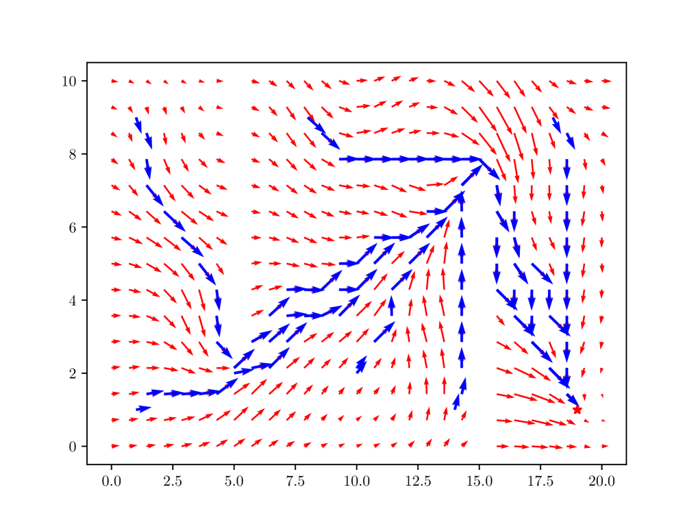
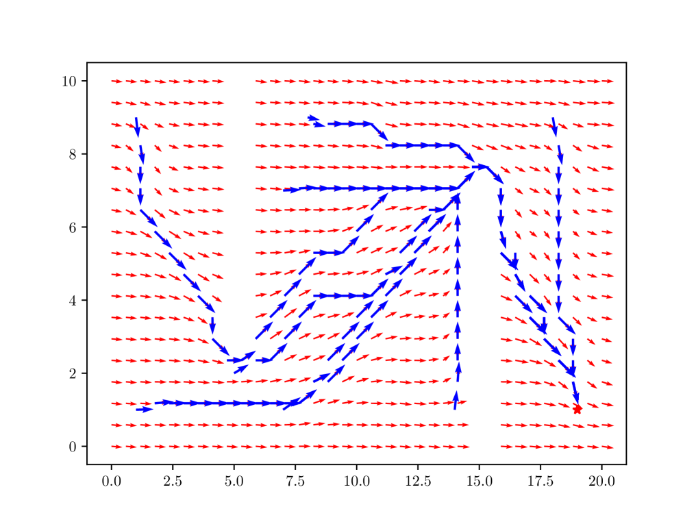
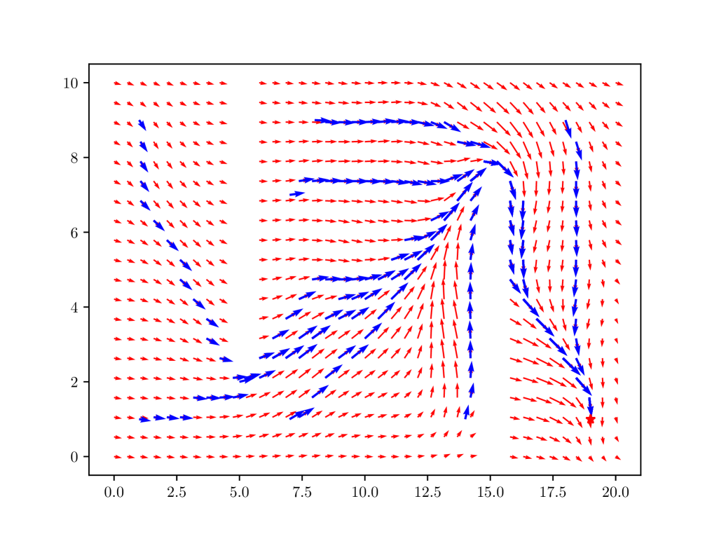
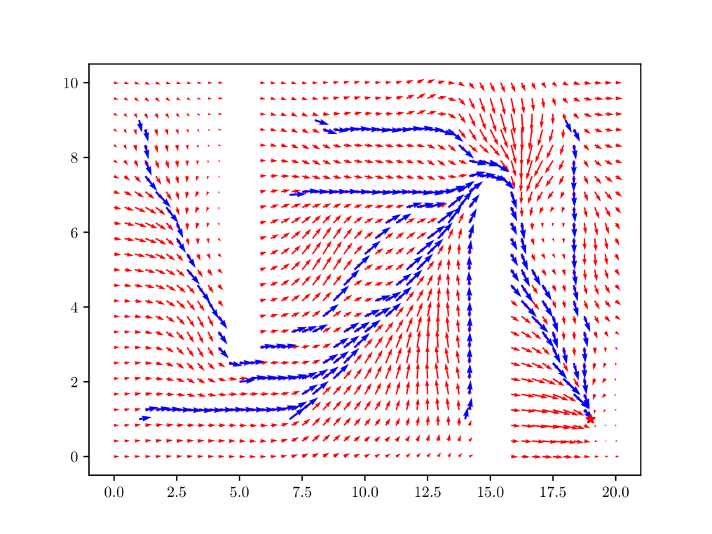
We consider a problem of automatic navigation of an agent [51]. We intend to navigate an agent starting from a given point to find a path to the goal without colliding into the obstacles. We sample grid points uniformly over the free space while avoiding the obstacle areas to construct a geometric graph structure involving the topological information. We first generate several trajectories with Dijkstra’s shortest path algorithm that leads the agent from a randomly selected starting point to the goal. Every point along the generated trajectories is labeled with a 2-d direction vector of the velocity. The geometric adjacency matrix is calculated based on the weight function defined in (14) with (21). Specifically, the underlying topology information is captured by setting the Euclidean distance between two points as infinity (i.e. weight value as zero) if there is no direct path connecting these two points without colliding into the obstacles. The input graph signal is the position coordinates of some point over the space and the final output is the direction that can lead to the goal point. The learned architectures are tested via randomly generating starting points and computing the trajectory by predicting directions of the points along the trajectory. If the trajectory can reach the goal point without colliding into the obstacles, the trajectory is marked as “success". The performances are measured by calculating the successful rates of all the learned architectures.
Learning architectures and experiment settings. We build dense geometric graphs as the approximations to the models as the regular grid graph structure brings little difference between the dense and sparse graph setting. We set the position of each point as input signals on the graphs. The weights of the edges are calculated based on the Euclidean distance between the nodes and the weight function is determined as (21) with . We calculate the Laplacian matrix for the graph as the input graph shift operator. We train and test three architectures, including 2-layer Graph Filters (GF), 2-layer Graph Neural Network (GNN) and 2-layer Lipschitz Graph Neural Network (Lipschitz GNN) which all contain input features, and features with filters in each layer. ReLU is used as the nonlinearity function in GNN and Lipschitz GNN. In Lipschitz GNN architecture, we put the Lipschitz continuity restriction to the graph filter function by importing a penalty term which is the scaled derivative of the filter function to the loss function. A larger Lipschitz constant indicates a smoother filter function. All architectures also include a linear readout layer to map the 2-d direction vector outputs. The loss function is MSE loss and the optimizer is SGD with the learning rate set as . The architectures are trained over epochs.
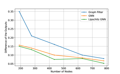
Convergence analysis. The convergence is tested by calculating the difference of the outputs of the graph filters in the last layer for each architecture. By training the graph filters and GNNs on geometric graphs with , and plotting the differences between the output of the trained graph filters or GNNs on geometric graphs with size and on the relatively large enough geometric graphs with size . From Figure 5 we can see that the output differences decrease and converge as the trained geometric graph size grows, which is accordant with Corollary 1. This also verifies the convergence of geoemtric GNNs as presented in 3 if we see the large geometric graph as an approximation of the underlying manifold. We can conclude that Lipschitz GNNs have better approximations while GNNs outperform Graph Filters.
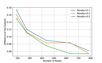
We further study the effect of Lipschitz continuity of the graph filter functions by changing the penalty constant . From Figure 3 we can see as the constant grows, the output differences become smaller, which attests our claim that smoother filter functions provide better approximations.
Transferability verification. We verify the transferability result presented in Corollary 1 by training the architectures on a sampled geometric graph with size and testing these architectures on the large geometric graphs with . Note that due to the non-scability of the linear readout layer, we keep the graph filter functions unchanged and only retrain the final linear layer to map the outputs to a 2-d direction vector. The successful rates are shown in Table I. We can observe that the architectures trained on smaller sampled geometric graphs can still perform well when implemented on larger graphs. Moreover, Lipschitz GNN performs slightly better than GNN which outperforms Graph Filters. This can be understood as the Lipschitz continuity of the filter functions and the nonlinearity functions help with the transferability as we have discussed in Section 3.
| Graph Filter | GNN | Lipschitz GNN | |
|---|---|---|---|
| 0.74 | 0.74 | 0.76 | |
| 0.79 | 0.8 | 0.78 | |
| 0.81 | 0.82 | 0.83 | |
| 0.82 | 0.83 | 0.84 |
To make the results more explicit, we show the predicted directions for each point over the space tested with a Lipschitz GNN trained on graph with in Figure 1. The red arrows point to the learned directions starting from each unlabeled points while the blue arrows are the learned directions for labeled points. We can see that Lipschitz GNN can efficiently learn the successful directions for unlabeled points based on these geometric graphs and can transfer to larger graphs.
VI-B Point Cloud Model Classification
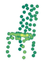
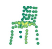
We further evaluate the convergence results on the ModelNet10 [52] classification problem. The dataset includes 3,991 meshed CAD models from 10 categories for training and 908 models for testing. In each model, points are uniformly randomly selected to construct geometric graphs to approximate the underlying model, such as chairs, tables. Figure 4 shows the point cloud model with different sampling points. Our goal is to identify the models for chairs from other models.


Learning architectures and experiment settings. We build both dense and sparse geometric graphs as the approximations to the models. We set the coordinates of each point as input signals on the graphs. The weights of the edges are calculated based on the Euclidean distance between the nodes. For the dense geometric graphs, the weight function is determined as (21) with . Similarly, the weight function of a sparse geometric graph is calculated as (24) with as the threshold. We calculate the Laplacian matrix for each graph as the input graph shift operator. In this experiment, we implement and compare three different architectures, including 2-layer Graph Filters (GF), 2-layer Graph Neural Network (GNN) and 2-layer Lipschitz Graph Neural Network (Lipschitz GNN). The architectures contain input features which are the 3-d coordinates of each point, and features with filters in each layer. In GNN and Lipschitz GNN, ReLU is used as the nonlinearity function. The filters in Lipschitz GNN is regularized as Lipschitz continuous by imposing a penalty term to the loss function with set as 0.3. All architectures include a linear readout layer to map the final classification outputs.
All the architectures are trained by minimizing the cross-entropy loss. We implement an ADAM optimizer with the learning rate set as 0.005 along with the forgetting factors 0.9 and 0.999. We carry out the training for 40 epochs with the size of batches set as 10. We run 5 random dataset partitions and show the average estimation error rates and the standard deviation across these partitions.
Convergence Verification. We verify our convergence results by training the graph filters and GNNs on geometric graphs with sampling points, and plotting the differences between the output of the trained graph filters or GNNs on geometric graphs with size and on the relatively large enough geometric graphs with size . Figure 5 shows the convergence results for dense graphs and figure 6 shows the results for sparse graphs.
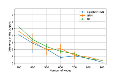
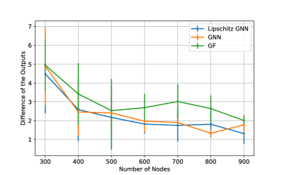
From the figures we can see that the differences between the outputs on the trained smaller geometric graphs and the relatively large geometric graphs decrease and converge as the trained graph size grows, which verifies Corollary 1. This also proves what we state in Theorem 3 that the approximation errors of geometric GNNs to the MNNs decrease as the number of nodes grows if we see the large enough graph with nodes as the manifold. We can also observe that Lipschitz GNNs have better approximations than GNNs because of the continuous filter function while GNNs outperform graph filters due to the nonlinearity function.
Transferability verification. We train the architectures on both dense and sparse geometric graphs with sampled points from each CAD model. To justify the theoretical results that we have stated in Section IV, we test these trained architectures on a relatively large graph containing sampled points to verify that geometric GNNs have the transferability to large graphs, i.e. the trained geometric graph filters and GNNs can be directly implemented on larger geometric graphs as long as the geometric graphs are constructed in the same manner. The classification error rates are shown in Table II for the dense graph setting and in Table III for the sparse graph setting.
| Graph Filters | GNN | Lipschitz GNN | |
|---|---|---|---|
| Graph Filters | GNN | Lipschitz GNN | |
|---|---|---|---|
We can see from the results shown in the tables that the trained architectures can still perform well on the relatively large geometric graphs, both for dense and sparse graph settings. We can see that Lipschitz GNNs outperform GNNs, which perform better than graph filters. This attests the effects of the filter function continuity and nonlinearity that we have discussed in Section IV, which is continuous filter function and nonlinearity function both help with improving transferability. We can also observe that architectures trained on geometric graphs with more number of nodes can achieve better performances on the relatively large graphs. This can be understood when we see this large enough geometric graph with approximately as the underlying manifold and as Theorem 3 shows the geometric GNNs can give better approximations to the MNNs as the number of nodes grow. This can also be understood as the transferability property presented in Corollary 1, which also indicates that graph filters and GNNs trained on larger geometric graphs have better performance approximations. Furthermore, the results also show that architectures trained on dense geometric graphs transfer better than the ones trained on sparse geometric graphs, which is also accordant with what we have claimed in Section IV.
VII Conclusions
In this paper, we import the definition of manifold convolutional filters with an exponential Laplace-Beltrami operator to process manifold signals. The manifold model is accessible with a set of i.i.d. uniformly sampled points over the manifold. We construct both dense and sparse graph models to approximate the underlying manifold. We first prove the approximation error bounds of discrete graph Laplacians to the LB operator in the spectral domain. We transfer the definition of manifold filter to the constructed graph and prove the graph filter can approximate the manifold filter with a non-asymptotic error bound. The constructed graph filters need to trade-off between the discrimative and approximative powers while GNNs composed with graph filters and nonlinearities can alleviate the trade-off with the frequency mixing by nonlinearities. We conclude that the GNNs are thus both good approximations of MNNs and discriminative. We finally verified our results numerically with a navigation control problem over a manifold.
References
- [1] Z. Wang, L. Ruiz, and A. Ribeiro, “Convolutional filtering on sampled manifolds,” in ICASSP 2023-2023 IEEE International Conference on Acoustics, Speech and Signal Processing (ICASSP). IEEE, 2023, pp. 1–5.
- [2] ——, “Convergence of graph neural networks on relatively sparse graphs,” 2023. [Online]. Available: https://zhiyangw.com/Papers/Asilomar2023.pdf
- [3] V. N. Ioannidis, A. G. Marques, and G. B. Giannakis, “Graph neural networks for predicting protein functions,” in 2019 IEEE 8th International Workshop on Computational Advances in Multi-Sensor Adaptive Processing (CAMSAP). IEEE, 2019, pp. 221–225.
- [4] V. Gligorijević, P. D. Renfrew, T. Kosciolek, J. K. Leman, D. Berenberg, T. Vatanen, C. Chandler, B. C. Taylor, I. M. Fisk, H. Vlamakis et al., “Structure-based protein function prediction using graph convolutional networks,” Nature communications, vol. 12, no. 1, pp. 1–14, 2021.
- [5] Q. Li, F. Gama, A. Ribeiro, and A. Prorok, “Graph neural networks for decentralized multi-robot path planning,” in 2020 IEEE/RSJ International Conference on Intelligent Robots and Systems (IROS). IEEE, 2020, pp. 11 785–11 792.
- [6] E. Tolstaya, J. Paulos, V. Kumar, and A. Ribeiro, “Multi-robot coverage and exploration using spatial graph neural networks,” in 2021 IEEE/RSJ International Conference on Intelligent Robots and Systems (IROS). IEEE, 2021, pp. 8944–8950.
- [7] J. Zeng, G. Cheung, M. Ng, J. Pang, and C. Yang, “3d point cloud denoising using graph laplacian regularization of a low dimensional manifold model,” IEEE Transactions on Image Processing, vol. 29, pp. 3474–3489, 2019.
- [8] M. Devanne, H. Wannous, S. Berretti, P. Pala, M. Daoudi, and A. Del Bimbo, “3-d human action recognition by shape analysis of motion trajectories on riemannian manifold,” IEEE transactions on cybernetics, vol. 45, no. 7, pp. 1340–1352, 2014.
- [9] Y. Wang, Y. Sun, Z. Liu, S. E. Sarma, M. M. Bronstein, and J. M. Solomon, “Dynamic graph cnn for learning on point clouds,” Acm Transactions On Graphics (tog), vol. 38, no. 5, pp. 1–12, 2019.
- [10] Z. He, L. Wang, H. Ye, G. Y. Li, and B.-H. F. Juang, “Resource allocation based on graph neural networks in vehicular communications,” in GLOBECOM 2020-2020 IEEE Global Communications Conference. IEEE, 2020, pp. 1–5.
- [11] Z. Wang, L. Ruiz, M. Eisen, and A. Ribeiro, “Stable and transferable wireless resource allocation policies via manifold neural networks,” in ICASSP 2022-2022 IEEE International Conference on Acoustics, Speech and Signal Processing (ICASSP). IEEE, 2022, pp. 8912–8916.
- [12] F. Gama, E. Isufi, G. Leus, and A. Ribeiro, “Graphs, convolutions, and neural networks: From graph filters to graph neural networks,” IEEE Signal Processing Magazine, vol. 37, no. 6, pp. 128–138, 2020.
- [13] A. Ortega, P. Frossard, J. Kovačević, J. M. Moura, and P. Vandergheynst, “Graph signal processing: Overview, challenges, and applications,” Proceedings of the IEEE, vol. 106, no. 5, pp. 808–828, 2018.
- [14] F. Scarselli, M. Gori, A. C. Tsoi, M. Hagenbuchner, and G. Monfardini, “The graph neural network model,” IEEE transactions on neural networks, vol. 20, no. 1, pp. 61–80, 2008.
- [15] F. Gama, A. G. Marques, G. Leus, and A. Ribeiro, “Convolutional neural network architectures for signals supported on graphs,” IEEE Transactions on Signal Processing, vol. 67, no. 4, pp. 1034–1049, 2019.
- [16] Z. Wang, L. Ruiz, and A. Ribeiro, “Convolutional neural networks on manifolds: From graphs and back,” arXiv preprint arXiv:2210.00376, 2022.
- [17] ——, “Stability of neural networks on manifolds to relative perturbations,” in ICASSP 2022-2022 IEEE International Conference on Acoustics, Speech and Signal Processing (ICASSP). IEEE, 2022, pp. 5473–5477.
- [18] J. Masci, D. Boscaini, M. Bronstein, and P. Vandergheynst, “Geodesic convolutional neural networks on riemannian manifolds,” in Proceedings of the IEEE international conference on computer vision workshops, 2015, pp. 37–45.
- [19] R. Chakraborty, J. Bouza, J. H. Manton, and B. C. Vemuri, “Manifoldnet: A deep neural network for manifold-valued data with applications,” IEEE Transactions on Pattern Analysis and Machine Intelligence, vol. 44, no. 2, pp. 799–810, 2020.
- [20] F. Gama, J. Bruna, and A. Ribeiro, “Stability properties of graph neural networks,” IEEE Transactions on Signal Processing, vol. 68, pp. 5680–5695, 2020.
- [21] N. Keriven, A. Bietti, and S. Vaiter, “Convergence and stability of graph convolutional networks on large random graphs,” Advances in Neural Information Processing Systems, vol. 33, pp. 21 512–21 523, 2020.
- [22] D. Zou and G. Lerman, “Graph convolutional neural networks via scattering,” Applied and Computational Harmonic Analysis, vol. 49, no. 3, pp. 1046–1074, 2020.
- [23] Z. Wang, L. Ruiz, and A. Ribeiro, “Stability to deformations of manifold filters and manifold neural networks,” arXiv preprint arXiv:2106.03725, 2021.
- [24] F. Monti, D. Boscaini, J. Masci, E. Rodola, J. Svoboda, and M. M. Bronstein, “Geometric deep learning on graphs and manifolds using mixture model cnns,” in Proceedings of the IEEE conference on computer vision and pattern recognition, 2017, pp. 5115–5124.
- [25] M. M. Bronstein, J. Bruna, Y. LeCun, A. Szlam, and P. Vandergheynst, “Geometric deep learning: going beyond euclidean data,” IEEE Signal Processing Magazine, vol. 34, no. 4, pp. 18–42, 2017.
- [26] M. Eliasof, E. Haber, and E. Treister, “Pde-gcn: novel architectures for graph neural networks motivated by partial differential equations,” Advances in neural information processing systems, vol. 34, pp. 3836–3849, 2021.
- [27] W. Shi and R. Rajkumar, “Point-gnn: Graph neural network for 3d object detection in a point cloud,” in Proceedings of the IEEE/CVF conference on computer vision and pattern recognition, 2020, pp. 1711–1719.
- [28] M. T. Kejani, F. Dornaika, and H. Talebi, “Graph convolution networks with manifold regularization for semi-supervised learning,” Neural Networks, vol. 127, pp. 160–167, 2020.
- [29] L. Ruiz, L. F. Chamon, and A. Ribeiro, “Transferability Properties of Graph Neural Networks,” arXiv preprint arXiv:2112.04629, 2021.
- [30] ——, “Graphon signal processing,” IEEE Transactions on Signal Processing, vol. 69, pp. 4961–4976, 2021.
- [31] J. Zhou, G. Cui, S. Hu, Z. Zhang, C. Yang, Z. Liu, L. Wang, C. Li, and M. Sun, “Graph neural networks: A review of methods and applications,” AI Open, vol. 1, pp. 57–81, 2020.
- [32] L. Ruiz, L. Chamon, and A. Ribeiro, “Graphon neural networks and the transferability of graph neural networks,” Advances in Neural Information Processing Systems, vol. 33, pp. 1702–1712, 2020.
- [33] S. Maskey, R. Levie, and G. Kutyniok, “Transferability of graph neural networks: an extended graphon approach,” arXiv preprint arXiv:2109.10096, 2021.
- [34] J. Calder and N. G. Trillos, “Improved spectral convergence rates for graph laplacians on epsilon-graphs and k-nn graphs,” arXiv preprint arXiv:1910.13476, 2019.
- [35] J. Chew, D. Needell, and M. Perlmutter, “A convergence rate for manifold neural networks,” arXiv preprint arXiv:2212.12606, 2022.
- [36] D. I. Shuman, S. K. Narang, P. Frossard, A. Ortega, and P. Vandergheynst, “The emerging field of signal processing on graphs: Extending high-dimensional data analysis to networks and other irregular domains,” IEEE signal processing magazine, vol. 30, no. 3, pp. 83–98, 2013.
- [37] A. Sandryhaila and J. M. Moura, “Discrete signal processing on graphs,” IEEE transactions on signal processing, vol. 61, no. 7, pp. 1644–1656, 2013.
- [38] N. Boumal, An introduction to optimization on smooth manifolds. Cambridge University Press, 2023.
- [39] S. Rosenberg and R. Steven, The Laplacian on a Riemannian manifold: an introduction to analysis on manifolds. Cambridge University Press, 1997, no. 31.
- [40] F. R. Chung, Spectral graph theory. American Mathematical Soc., 1997, vol. 92.
- [41] J. Pach, “The beginnings of geometric graph theory,” Erdős Centennial, pp. 465–484, 2013.
- [42] R. Merris, “A survey of graph laplacians,” Linear and Multilinear Algebra, vol. 39, no. 1-2, pp. 19–31, 1995.
- [43] R. Levie, W. Huang, L. Bucci, M. Bronstein, and G. Kutyniok, “Transferability of spectral graph convolutional neural networks,” Journal of Machine Learning Research, vol. 22, no. 272, pp. 1–59, 2021.
- [44] D. B. Dunson, H.-T. Wu, and N. Wu, “Spectral convergence of graph laplacian and heat kernel reconstruction in from random samples,” Applied and Computational Harmonic Analysis, vol. 55, pp. 282–336, 2021.
- [45] M. Belkin and P. Niyogi, “Towards a theoretical foundation for laplacian-based manifold methods,” Journal of Computer and System Sciences, vol. 74, no. 8, pp. 1289–1308, 2008.
- [46] Y. Shi and B. Xu, “Gradient estimate of an eigenfunction on a compact riemannian manifold without boundary,” Annals of Global Analysis and Geometry, vol. 38, no. 1, pp. 21–26, 2010.
- [47] A. Seelmann, “Notes on the theorem,” Integral Equations and Operator Theory, vol. 79, no. 4, pp. 579–597, 2014.
- [48] M. Penrose, Random geometric graphs. OUP Oxford, 2003, vol. 5.
- [49] M. Hamidouche, “Spectral analysis of random geometric graphs,” Ph.D. dissertation, Université Côte d’Azur, 2020.
- [50] W. Arendt and W. P. Schleich, Mathematical analysis of evolution, information, and complexity. John Wiley & Sons, 2009.
- [51] J. Cervino, L. Chamon, B. D. Haeffele, R. Vidal, and A. Ribeiro, “Learning globally smooth functions on manifolds,” arXiv preprint arXiv:2210.00301, 2022.
- [52] Z. Wu, S. Song, A. Khosla, F. Yu, L. Zhang, X. Tang, and J. Xiao, “3d shapenets: A deep representation for volumetric shapes,” in Proceedings of the IEEE conference on computer vision and pattern recognition, 2015, pp. 1912–1920.
- [53] U. Von Luxburg, M. Belkin, and O. Bousquet, “Consistency of spectral clustering,” The Annals of Statistics, pp. 555–586, 2008.
- [54] M. Belkin and P. Niyogi, “Convergence of laplacian eigenmaps,” Advances in neural information processing systems, vol. 19, 2006.
Appendix A Appendix
A-A Proof of Theorem 1 and Theorem 2
We first write out the filter representation as
| (37) |
We denote the index of partitions that contain a single eigenvalue as a set () and the rest as a set (). We decompose the -FDT filter function as as
| (40) | ||||
| (44) |
with some constant in . With the triangle inequality, we start by analyzing the output difference of as
| (45) |
The first term in (45) can be bounded by leveraging the -Lipschitz continuity of the frequency response. From the eigenvalue difference in Proposition 4, we can claim that for each eigenvalue , we have
| (46) |
The square of the first term is bounded as
| (47) | |||
| (48) |
The second term in (45) can be bounded combined with the convergence of eigenfunctions in (50) as
| (49) |
From the convergence stated in Theorem 4, we have
| (50) |
with the eigengap under the -FDT filter. Therefore, the first term in (49) can be bounded as
| (51) |
The last equation comes from the definition of norm in . The second term in (49) can be written as
| (52) |
Because is a set of uniform sampled points from , based on Theorem 19 in [53] we can claim that
| (53) |
Taking into consider the boundedness of frequency response and the bounded energy . Therefore, we have
Combining the above results, we can bound the output difference of . Then we need to analyze the output difference of and bound this as
| (54) |
where and are filters with filter function on the LB operator and graph Laplacian respectively. Combining the filter functions, we can write
| (55) | |||
| (56) | |||
With , we have
| (57) |
We can prove Theorem 2 similarly by importing Proposition 4 into the eigenvalue and eigenfunction differences.
Supplemental Materials
Appendix B Supplementary Materials
B-A Proof of Proposition 1
We decompose the operator difference between the graph Laplacian and the LB operator with an intermediate term , which is the functional approximation defined in (20). We first focus on the operator difference between and . From [45], we can get the bound as
| (58) |
For the Sobolev norm of eigenfunction , according to [54, Lemma 4.4] we have
| (59) |
which leads to
| (60) |
For the operator difference between and with Hoeffding’s inequality as
| (61) |
Therefore, we can claim that with probability at least , we have
| (62) |
Combining (60) and (62) with triangle inequality, we can get the conclusion in Theorem 1.
B-B Proof of Proposition 2
We first import two lemmas to help prove the spectral properties.
Lemma 2
Let be self-adjoint operators with and as the corresponding spectrum. Let be the orthogonal projection operation onto the subspace generated by . Then we have
| (63) |
Proof.
The first inequality is directly from [53, Proposition 18]. Let be the orthogonal projection onto the complement of the subspace generated by . Then we have
| (64) |
Therefore, we have
| (65) | |||
| (66) | |||
| (67) | |||
| (68) | |||
| (69) |
together with . We can conclude the proof. ∎
The following lemma is adapted from [44, Lemma 5c]
Lemma 3
Let be self-adjoint operators with and as the corresponding spectrum. Then we have
| (70) |
With the above lemmas and our proposed Theorem 1, which includes the operator difference, we can prove Theorem 2. We first fix some , wich provides an upper bound for for all . By taking the probability and , we can conclude that the operator difference in Theorem 1 can be bounded with order , with the constant scaling with . Combine with Lemma 2 and , we can get
| (71) |
where we denote the constant as to include the effects of , the eigengap and the volume of .
This upper bound of the eigenfunction difference leads to . Combining with Lemma 3, the difference of the eigenvalues can also be bounded in the order of .
B-C Proof of Theorem 3
To bound the output difference of MNNs, we need to write in the form of features of the final layer
| (72) |
By inserting the definitions, we have
| (73) |
with as the input of the first layer. With a normalized point-wise Lipschitz nonlinearity, we have
| (74) | ||||
| (75) |
The difference can be further decomposed as
| (76) | ||||
| (77) |
The second term can be bounded with . The first term can be decomposed by Cauchy-Schwartz inequality and non-amplifying of the filter functions as
| (78) |
where representing the constant in the error bound of manifold filters in (2). To solve this recursion, we need to compute the bound for . By normalized Lipschitz continuity of and the fact that , we can get
| (79) |
Insert this conclusion back to solve the recursion, we can get
| (80) |
Replace with we can obtain
| (81) |
With and for , then we have
| (82) |
which concludes the proof.