Multiwavelength variability of $\gamma$-ray emitting narrow-line Seyfert 1 galaxies

Abstract

As one of the drivers of feedback in active galactic nuclei (AGNs), the jets launched from supermassive black holes (SMBHs) are important for understanding the co-evolution of SMBHs and their host galaxies. However, the formation of AGN jets is far from clear. The discovery of $\gamma$-ray narrow-line Seyfert 1 (NLS1) galaxies during the past two decades has provided us with a new means of studying the link between jets and accretion processes and the formation of jets. Here we explore the coupling of jet and accretion discs in seven bright $\gamma$-ray NLS1 galaxies by studying simultaneous optical/UV and X-ray observations of these systems taken by Swift. The results show that, except for 1H 0323+342 in which the X-rays are significantly contributed from the accretion disc, the observed X-ray emission of the other sources is dominated by the jet, and the accretion process makes little contribution if not absent. Although the origin of the X-ray emission is different, the broad-band spectral shape characterized by $\alpha_{\rm ox}$ and the X-ray flux is found to follow the same evolutionary trend in 1H 0323+342, PMN J0948+0022, and PKS 1502+036. For the remaining sources, the trend is not observed or the sampling is not dense enough.

1 Introduction

Powered by supermassive black holes (SMBHs, in the mass range 10${}^{6}$–10${}^{10}$ $\rm{M}_{\odot}$) at their centers, active galactic nuclei (AGNs) are among the most luminous long-lived sources in the universe. Collimated outflows of matter in form of jets, launched from the vicinity of the central accreting SMBH, are found in many AGNs. Jets and outflows are suggested to be one of the fundamental mechanisms by which the SMBH interacts with the host galaxy, regulating its evolution (DiMatteo2005; Wagner2012). However, the physical mechanism of jet formation and the role of black hole mass, magnetic fields and accretion disc properties are still not well understood (Blandford2019). The energetic particles in AGNs emit radiation at radio frequencies via the synchrotron process and make their jets detectable as luminous radio sources. But only less than 20 percent of all AGNs are found to be radio-loud (1995PASP..107..803U; 2002AJ....124.2364I), while the rest are radio-quiet. The majority of the radio-quiet sources do have faint jets, and only few AGNs are not detected at all in the radio regime. However, the question is still open as to which parameters drive the most powerful, bright, relativistic jets in the radio-loud population in particular.

The conventional picture established during the first few decades after the discovery of radio quasar was that the relativistic AGN jets are preferentially associated with the heavier SMBHs residing in giant elliptical/bulge-dominated galaxies (1997ApJ...479..642B; 2003MNRAS.340.1095D; 2004MNRAS.355..196F). This knowledge has been updated by the discoveries in the last two decades of samples of radio-loud narrow-line Seyfert 1 (NLS1) galaxies and the more massive radio-loud narrow-line type 1 quasars (2006AJ....132..531K) that showed SMBH masses below 10${}^{8}$ M${}_{\odot}$, below the classical radio-loud regime. The vast majority of the latter still lacks host images, but among the very small number of them that do have host imaging, a few disc-like galaxies have been identified (e.g. 2007ApJ...658L..13Z; 2018A&A...619A..69J; 2020MNRAS.492.1450O).

In particular, some radio-loud NLS1 galaxies show persistent or flaring $\gamma$-ray emission independently re-confirming their launch of powerful relativistic jets (e.g. 2009ApJ...699..976A; 2009ApJ...707L.142A). The presence of such jets was already earlier found from radio observations (e.g., 2006AJ....132..531K; 2008ApJ...685..801Y). NLS1 galaxies generally host less massive but rapidly growing SMBHs and NLS1s galaxies are suggested to be located at the end of the AGN parameter space opposite to the classical blazars (2002ApJ...565...78B). Thus, NLS1 galaxies provide us with new laboratories for studying open questions related to the formation and evolution of relativistic jets in AGNs.

For this study, we selected bright radio-loud, gamma-ray detected NLS1 galaxies with multiyear coverage obtained by the Neil Gehrels Swift observatory (Swift hereafter; Gehrels2004). The targets of our study (Table 1) have been studied in selected time intervals and/or wavebands before (e.g., 2010ApJ...715L.113L; 2011MNRAS.413.2365C; 2012ApJ...759L..31J; 2012A&A...548A.106F; 2013ApJ...773...85E; 2013ApJ...775L..26I; 2015AJ....150...23Y; 2015MNRAS.454L..16Y; Foschini2015; 2018rnls.confE..42G; 2018A&A...618A..92A; 2018MNRAS.477.5127Y; 2019MNRAS.487L..40Y; 2020MNRAS.496.2213D; 2020MNRAS.498..859D; 2021A&A...654A.125B; 2021ApJS..255...10M; 2022MNRAS.tmp.1571O). Here, we combine archival Swift data and our own Swift data until 2021 December. Focus is on recent data since 2019, but we also add pre-2019 data to the analysis, for comparison purposes and in order to identify systematic trends. In particular, we address the broad-band spectral evolution using the simultaneous optical/UV and X-ray observations obtained by the X-ray telescope (XRT; 2005SSRv..120..165B) and ultra-violet–optical telescope (UVOT; 2005SSRv..120...95R) onboard Swift. We note that several of the sources in our study are formally quasars, however, for simplicity we continue to refer to all of them as "Seyfert" galaxies hereafter, as is a common habit when discussing NLS1 galaxies.

This paper is structured as follows: In Section 2 we describe the data reduction for the XRT and UVOT, respectively. The results and the analysis based on the optical/UV and X-ray data are provided in Section 3. In Section LABEL:sec:discussion we discuss the results of the Swift observations and finally a brief summary is given in Section LABEL:sec:summary. Throughout this work, we use a cosmology with $H_{\rm 0}$=70 km s${}^{-1}$ Mpc${}^{-1}$, $\Omega_{\rm M}$=0.3 and $\Omega_{\rm\Lambda}$=0.7.

Table 1: Summary of the $\gamma$-ray NLS1 galaxies in our study.

Name	R.A.	Dec.	$z$	$\gamma$-ray detection	BH mass	BH mass
	(J2000)	(J2000)		Ref.	[10${}^{7}$ $\rm{M}_{\odot}$]	Ref.
(1)	(2)	(3)	(4)	(5)	(6)	(7)
1H 0323+342	03:24:41.16	+34:10:45.9	0.063	1	${3.4}$	1
SDSS J094635.06+101706.1	09:46:35.07	+10:17:06.1	1.004	1	19	1
PMN J0948+0022	09:48:57.32	+00:22:25.6	0.584	1	4	1
SDSS J122222.55+041315.7	12:22:22.55	+04:13:15.8	0.966	1,1	20	1
PKS 1502+036	15:05:06.48	+03:26:30.8	0.408	1	0.4	1
PKS 2004$-$447	20:07:55.18	$-$44:34:44.2	0.24	1	7	1
SDSS J211852.96$-$073227.5	21:18:52.96	$-$07:32:27.6	0.260	1,1	3.4	1

Notes. Column (1): source name. Column (2) and (3): right ascension (R.A.) and declination (Dec.) of the galaxy. Column (4): redshift. Column (5): References for the $\gamma$-ray detection of the source. Column (6) and (7): black hole mass and reference. References: (1) 2009ApJ...707L.142A; (1)2010ApJS..188..405A; (1) 2009ApJ...699..976A; (1) 2015MNRAS.454L..16Y; (1) 2018MNRAS.477.5127Y; (1)2018ApJ...853L...2P; (1) 2016ApJ...824..149W; (1) 2019MNRAS.487L..40Y; (1) 2003ApJ...584..147Z; (1) 2008ApJ...685..801Y; (1) 2021A&A...649A..77G;

2 Swift Observations and data reduction

2.1 XRT

2.1.1 Data reduction

Data taken with the Swift/XRT are reprocessed following standard procedures using the task xrtpipeline. The photon counting (PC) mode (2004SPIE.5165..217H) data are selected for the analysis. The images are extracted first and visually inspected to exclude those observations in which the source is at the edge or outside of the field of view. To obtain the spectra, the source counts are extracted from a circle of 50″ radius centered on the source position and the background is estimated from an annulus with inner radius of 60″ and three times the area of the source region, except for 1H 0323+342 which sometimes has brightened to a count rate higher than 0.5 counts s${}^{-1}$. These data are affected by pile-up. In order to determine at which point the data and the XRT point spread function (PSF) model diverge, the XRT image from the observation in which 1H 0323+342 has highest count rate is modeled by a King function $\text{PSF}(r)=\left[1+(r/r_{\rm c})^{2}\right]^{\beta}$, where $r_{\rm c}=5.8$, $\beta=1.55$ and $r$ is the distance to the PSF center. The King function is fitted to the outer wings of the PSF at distance larger than 15″. The best-fit model is then visually compared with the data, and the diverge appears below $\sim$8″. Thus, for all the XRT observations on 1H 0323+342 with count rate $>0.5$ counts s${}^{-1}$ the source events are extracted from an annulus with inner/outer radius of 8″/60″, and the backgrounds are estimated from an annulus with inner/outer radius of 70″/90″.

The observations in which the sources are not detected ($<5\sigma$) are excluded. Full grade selection (0–12) is adopted to extract the source and background spectra. The ancillary response files are built using task xrtmkarf with the corresponding exposure maps to correct the PSF if any. The relevant response matrix files given in the output of xrtmkarf are used. The spectra with more than 125 counts are grouped such that they have at least 25 counts in each bin, and the $\chi^{2}$ minimization is used to fit model to the spectra. For the spectra with 125 or less counts, the spectra are grouped such that each spectrum has 5 to 10 bins, and the Cash statistic is adopted to fit the spectra. The software package XSPEC (1996ASPC..101...17A) was used for spectral analysis. A summary of the X-ray observations used in our analysis is given in Table 2.

2.1.2 Spectral fitting and flux estimation

All the spectra with 125 or less counts, and most of the spectra with more than 125 counts can be well fitted by a single power law with Galactic neutral hydrogen absorption, except for some spectra of 1H 0323+342 when the $\chi^{2}$-minimization gives a very poor, unacceptable fit, indicating an extra component other than a single power law is required. The spectra revealing a $\chi^{2}$ higher than the 90% quantile of the $\chi^{2}$ distribution given their degrees of freedom (dof) are then selected and fitted with a blackbody component plus a single power-law model. The absorption is fixed at the Galactic value and the blackbody temperature is forced to be in the range of $0.03\,\text{keV}<\text{Tk}<0.2\,\text{keV}$ during the fitting. The absorption-corrected flux is estimated by cflux. The fluxes in the 0.3–2 keV band ($f_{\rm soft}$) and 2–10 keV ($f_{\rm hard}$) band of the sources are shown in Figure 1–7. A summary of the results obtained from XRT observations is given in Table 3.

Table 2: Summary of the Swift observations.

Name	Time	X-ray		$N_{\rm obs}$ of optical/UV
	Coverage	$N_{\rm obs}$	Exp. (s)	$v$	$b$	$u$	$w1$	$m2$	$w2$
(1)	(2)	(3)	(4)	(5)	(6)	(7)	(8)	(9)	(10)
1H 0323+342	2006 Jul 05 – 2021 Jul 11	149	74 – 8821	113	97	105	107	102	123
SDSS J094635.06+101706.1	2019 May 25 – 2019 Jun 01	2	1743 – 1875	0	0	1	2	2	2
PMN J0948+0022	2008 Dec 05 – 2021 Nov 20	70	187 – 7754	34	51	73	52	50	53
SDSS J122222.55+041315.7	2007 Aug 05 – 2011 Jun 24	6	1561 – 9178	3	4	5	3	4	3
PKS 1502+036	2009 Jul 25 – 2020 Sep 17	59	631 – 5157	6	36	47	55	57	58
PKS 2004$-$447	2011 May 15 – 2019 Nov 13	39	714 – 12 180	7	10	21	14	9	13
SDSS J211852.96$-$073227.5	2019 May 05 – 2019 Oct 22	8	1204 – 3771	4	1	4	1	0	5

Notes. Column (1): source name. Column (2): time coverage of the Swift observations. Column (3) and (4): number of the X-ray observations and the range of exposure times of the X-ray observations. Column (5)–(10): number of the optical/UV observations in $v$, $b$, $u$, $w1$, $m2$ and $w2$ band, respectively. We note that $N_{\rm obs}$ refers to the number of observations used in the following analysis, excluding observations with no detection.

Figure 1: Swift light curve of 1H 0323+342. The time along the x-axis is not continuous. Time intervals without any data were removed for visual clarity. The vertical grey lines in the figure mark the boundaries of each time windows in which there exist observed data. Upper panel: light curve in the $v$, $b$, $u$, $w1$, $m2$ and $w2$ bands in units of magnitude. The magnitudes of the source are offset for visual clarity and are not corrected for Galactic extinction. Lower panel: The X-ray flux is reported in the 0.3–2 keV band (red points) and the 2–10 keV band (blue points). The red dotted lines mark the higher and lower flux thresholds, above and below which the high and low states are selected based on 0.3–2 keV X-ray fluxes. The light blue shaded areas mark the epochs selected for X-ray spectral stacking (see Section 3.3).

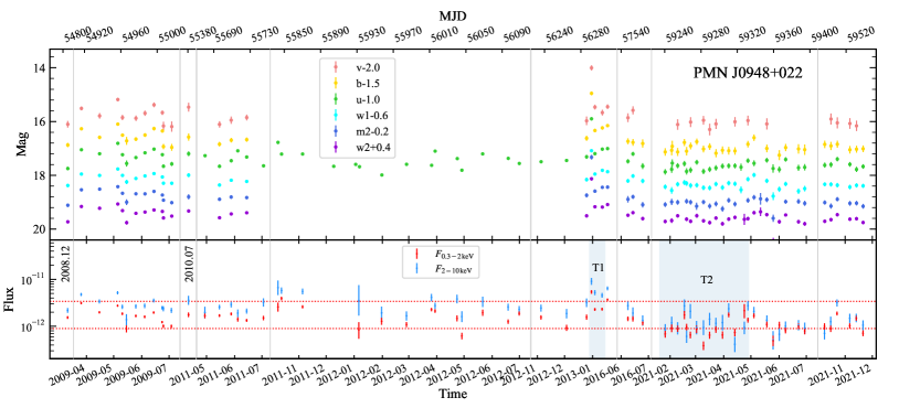
Figure 2: Same as Figure 1 but for PMN J0948+0022.

Figure 3: Same as Figure 1 but for PKS 1502+036.

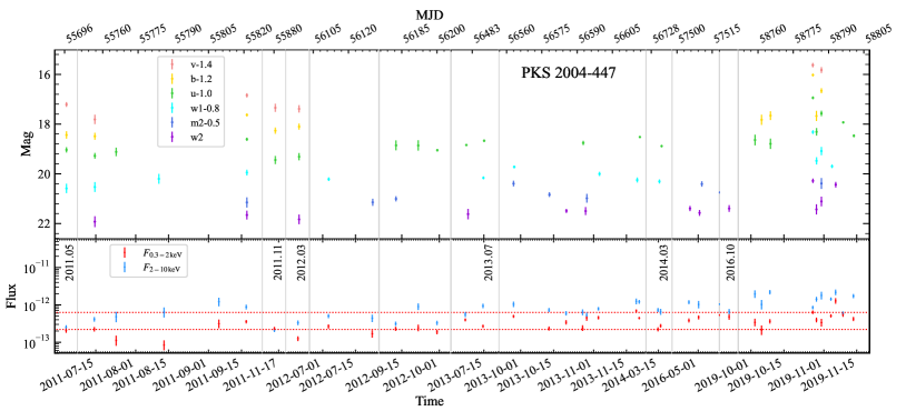
Figure 4: Same as Figure 1 but for PKS 2004-447.

Figure 5: Light curve of J0946+1017. Upper panel: light curve in the $u$, $w1$, $m2$ and $w2$ bands in units of magnitude. The magnitudes of the source are offset for visual clarity and are not corrected for extinction. Lower panel: The X-ray flux in 0.3–2 keV (red) and 2–10 keV (blue).

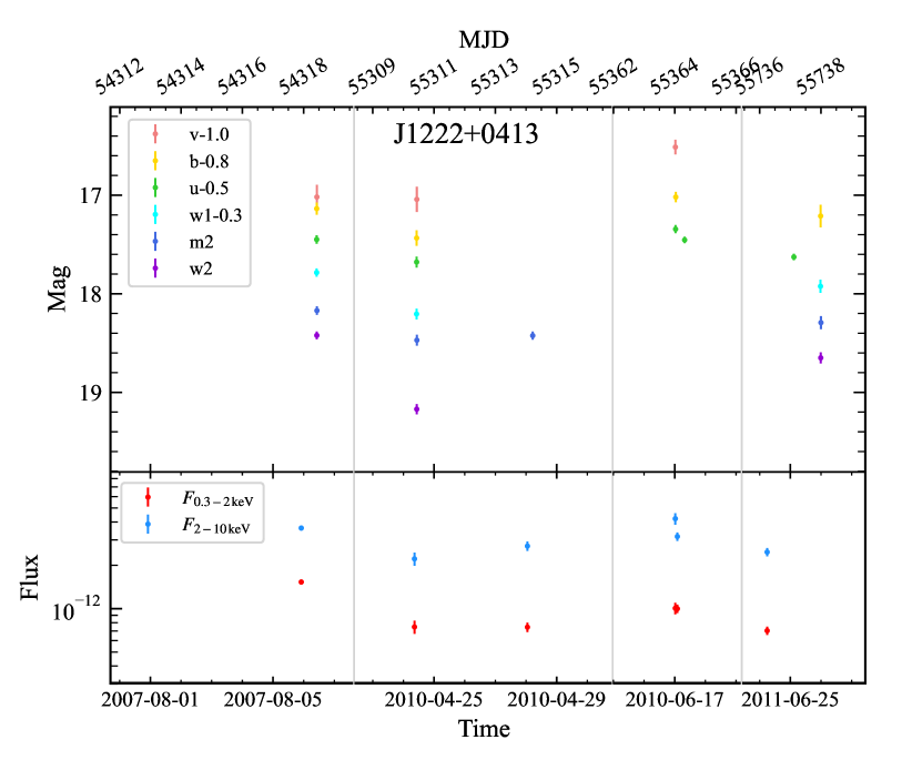
Figure 6: Light curve of SDSS J1222+0413. Upper panel: light curve in the $v$, $b$, $u$, $w1$, $m2$ and $w2$ bands in units of magnitude. The magnitudes of the source are offset for visual clarity and are not corrected for extinction. Lower panel: The X-ray flux light curve in 0.3–2 keV and 2–10 keV.

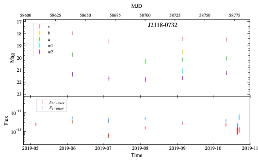
Figure 7: Light curve of SDSS J2118$-$0732. Upper panel: light curve in the $v$, $b$, $u$, $w1$ and $w2$ bands in units of magnitude. The magnitudes of the source are not corrected for extinction. Lower panel: The X-ray flux light curve in 0.3–2 keV and 2–10 keV.

2.2 UVOT

The NLS1 galaxies of this study have also been observed with the Swift/UVOT, in up to all three optical and up to all three UV bands [with filters: $v$ (5468Å), $b$ (4392Å), $u$ (3465Å), $w1$ (2600Å), $m2$ (2246Å), and $w2$ (1928Å), where values in brackets represent the filter central wavelengths (2008MNRAS.383..627P)]. Some sources have only been observed in selected bands. For each observation, data in each filter are co-added using the task uvotimsum after aspect correction. The images are visually inspected to exclude those in which the source is on the edges or out of the field of view. The source counts in each available filter were extracted in a circle with radius of 5″, while the background was selected in a nearby source-free region of radius 15″. The background-corrected counts are then converted into fluxes based on the latest calibration as described by 2008MNRAS.383..627P and 2010MNRAS.406.1687B using the task uvotsource. A summary of the UVOT observations and results are given in Table 2 and Table 3, respectively. The total duration of each UVOT observation is the same as the corresponding XRT duration. Each UVOT band $v$:$b$:$u$:$w1$:$m2$:$w2$ is observed with a ratio of 1:1:1:2:3:4 of the total exposure time, respectively. Correction of the UVOT fluxes for Galactic reddening towards the individual NLS1 galaxies was carried out using the values of $E_{\rm{(B-V)}}$ from 2011ApJ...737..103S and the reddening curves of 1999PASP..111...63F. We use the extinction-corrected optical/UV flux in the following analysis unless mentioned otherwise.

Table 3: Swift results.

Name	Variability				$\Gamma$	$L_{\rm X,peak}$		$\alpha_{\rm UV}$	$\alpha_{\rm ox}$
	optical	UV	X${}_{\rm soft}$	X${}_{\rm hard}$		soft	hard
						[$10^{44}$ $\rm erg\,s^{-1}$]
(1)	(2)	(3)	(4)	(5)	(6)	(7)	(8)	(9)	(10)
1H 0323+342	1.4	2.1	6.6	8.2	(1.1, 2.4)	2.3	2.0	($-0.34$, 0.01)	(1.14, 1.38)
SDSS J094635.06+101706.1	$\dots$	1.2	1.2	1.7	(1.9, 2.1)	15.6	16.2	(1.26, 1.74)	(1.20, 1.28)
PMN J0948+0022	$>$8.5	15.1	14.0	21.9	(1.1, 2.3)	77.5	130.2	($-0.40$, 0.02)	(1.02, 1.30)
SDSS J122222.55+041315.7	1.6	2.0	2.2	1.9	(1.0, 1.4)	76.1	209.6	($-0.42$, 0.08)	(1.13, 1.21)
PKS 1502+036	2.1	2.0	3.8	47.4	(0.4, 2.9)	1.8	11.9	($-0.49$, 0.06)	(1.15, 1.48)
PKS 2004$-$447	7.5	$>$5.6	15.2	10.3	(0.7, 1.9)	2.2	3.8	(1.39, 2.98)	(0.84, 1.17)
SDSS J211852.96$-$073227.5	$>$1.9	1.6	5.3	3.2	(0.8, 1.9)	0.7	1.2	(0.73, 1.25)	1.20

Notes. Column (1): source name. Column (2) to (5): factor of flux variation in the optical, UV, soft X-rays (0.3–2 keV) and hard X-rays (2–10 keV), respectively. A lower limit on the variability in the optical or UV is obtained when a flux upper limit given by uvotsource is lower than all the detections. Column (6): X-ray photon index range from spectral fitting. Column (7) and (8): isotropic X-ray peak luminosity in the soft and hard X-ray band, respectively, in units of $10^{44}$ $\rm erg\,s^{-1}$. Column (9): spectral index between optical and UV, $\alpha_{\rm uv}$, where $f_{\nu}\propto\nu^{-\alpha_{\rm uv}}$, calculated using the $v$ band and the $w2$ band. When there is no or too few $v$ or $w2$ data, a nearby band is used (see Section 3.2). Column (10): $\alpha_{\rm ox}$ calculated using the extinction corrected flux density at the $w1$ band and at 2 keV.

3 Results

3.1 Broadband spectral slope $\alpha_{\rm ox}$

To quantify the broadband spectral slope, the spectral index $\alpha_{\rm ox}$ between optical/UV and X-ray is calculated as $\alpha_{\rm ox}=-0.384\log\left(f_{2500}/f_{2\rm\,keV}\right)$, where $f_{2500}$ and $f_{2\rm\,keV}$ are the flux densities at 2500 Å and 2 keV, respectively. Here the flux density obtained from $w1$ band centered at $\sim 2600$ Å is adopted. The flux density at 2 keV is obtained from the best-fit model to each XRT spectrum.

To explore the broadband spectral slope variation along with the flux, we show the $\alpha_{\rm ox}$ vs. flux for 1H 0323+342, PMN J0948+0022, PKS 1502+0362 and PKS 2004-447 in Figure 8. The other three sources are not shown because they were observed only for a few times simultaneously in $w1$ and X-rays. As can be seen, although with large uncertainties there is a clear trend of softer $\alpha_{\rm ox}$ with decreasing X-rays flux in 1H 0323+342 and PMN J0948+0022. In PKS 1502+0362, this trend is still obvious for the hard X-rays, but vanishes for the X-rays below 2 keV. In PKS 2004-447, there is no clear trend for both soft and hard X-rays.

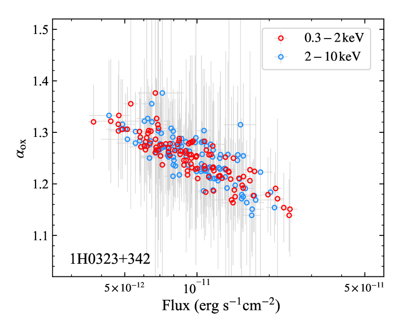
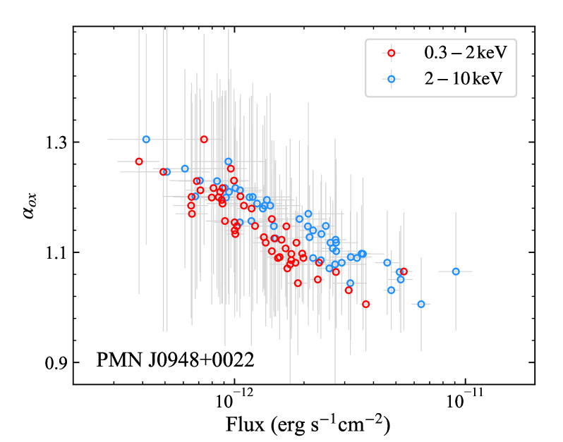
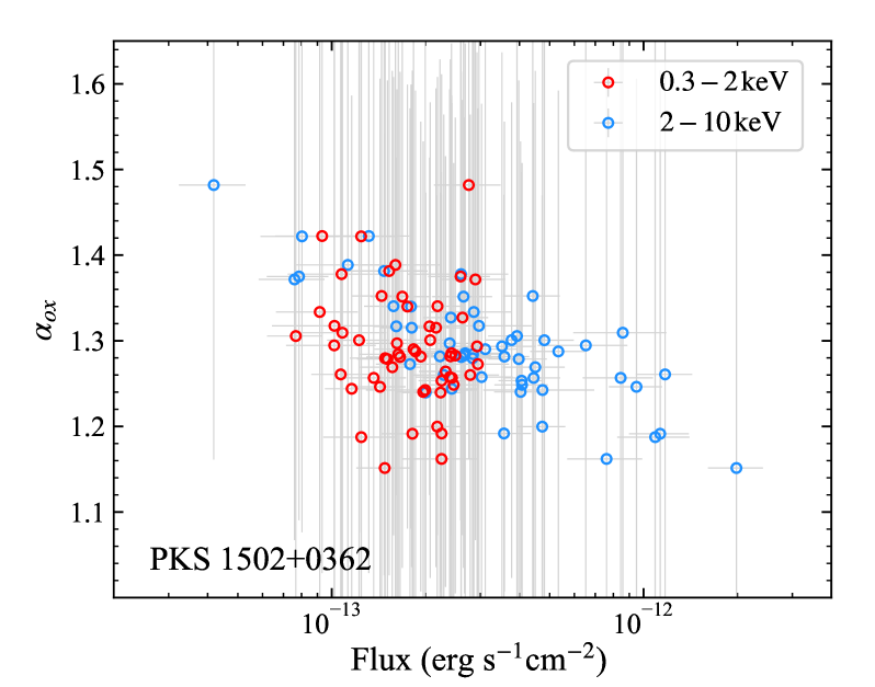
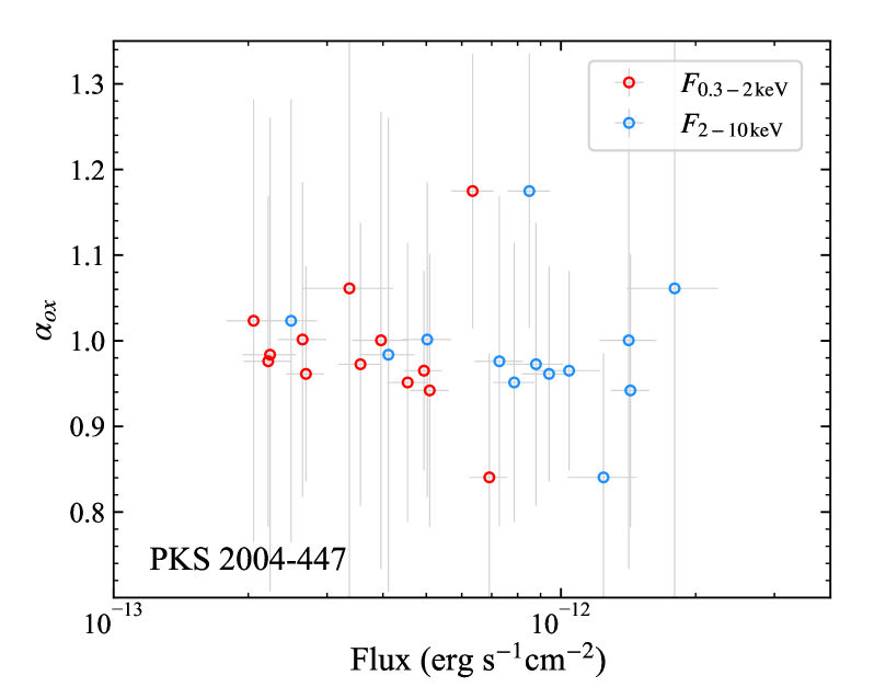
Figure 8: The $\alpha_{\rm ox}$ versus the X-ray flux for 1H 0323+342 (upper left), PMN J0948+0022 (upper right), PKS 1502+036 (lower left) and PKS 2004-447 (lower right). The X-ray flux in 0.3–2 keV and 2–10 keV are colored by red and blue, respectively. The error bars are colored in grey.

3.2 UV–X-ray SEDs

For visually inspecting the correlation between the evolution of optical/UV and X-ray spectra, we build the spectral energy distributions for these sources with, if any, the UVOT data and the best-fit model of the simultaneous X-ray spectra in the same colors (Figure 9). Data are represented as simple powerlaw connections between the respective UVOT fluxes: For 1H 0323+342, PMN J0948+0022 and SDSS J2118$-$0732, the extinction-corrected $v$ and $w2$ band data are used. For SDSS J1222+0413, the $b$ band is used instead of $v$ as there is only two $v$-band exposures. For PKS 1502+036 and PKS 2004-447, the $b$ and $u$ band data are used, respectively, as the data points in other optical band are too few. For SDSS J0946+1017, the $w1$ and $w2$ band data are used as in the optical band this source is only detected in the $u$ band in one of the observations by Swift.

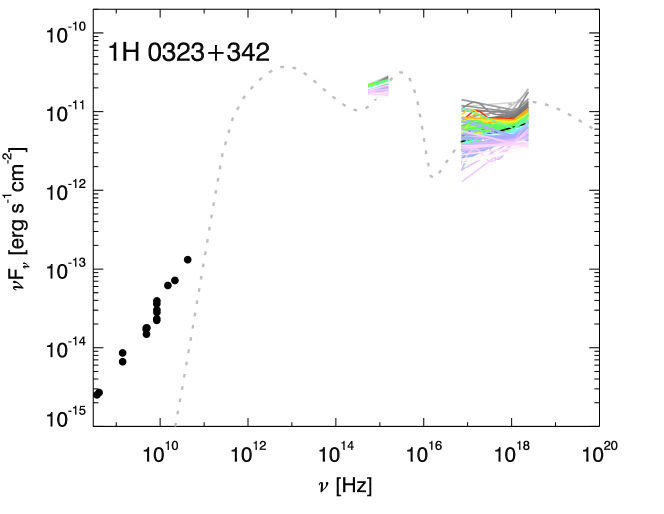
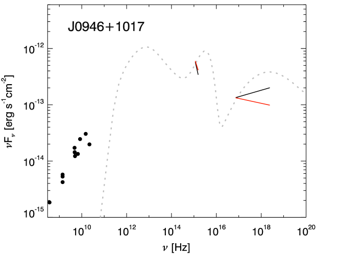
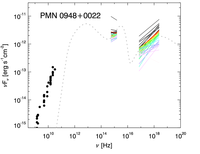
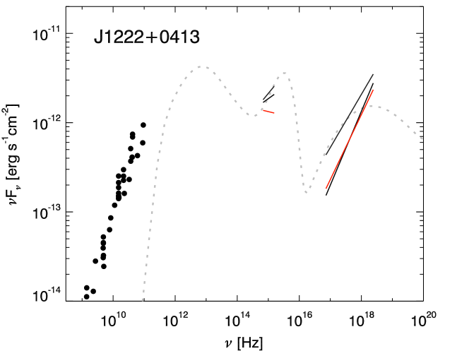
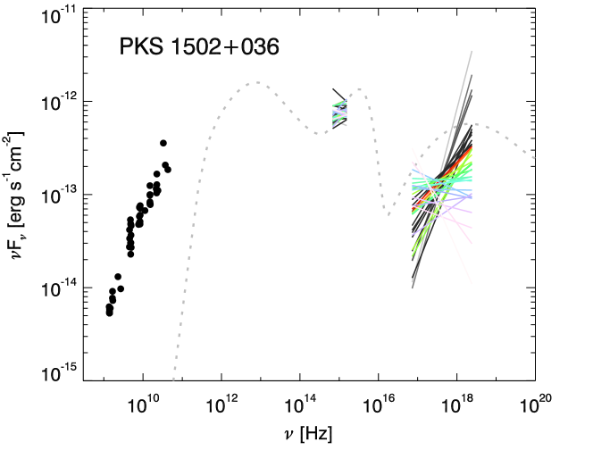
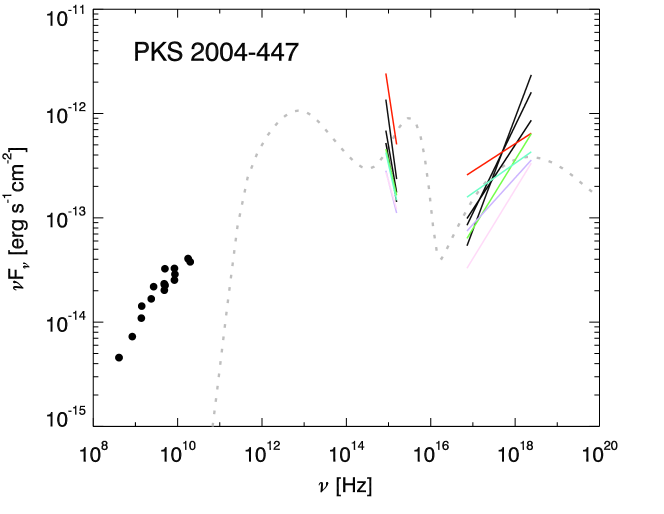
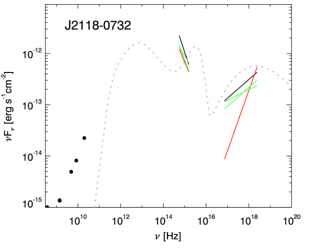
Figure 9: SEDs of the $\gamma$-ray NLS1 galaxies in our sample, built using simultaneous Swift UVOT and XRT data in the observer’s frame. Simultaneous UVOT/XRT data are marked in the same colour. The UVOT data are corrected for Galactic extinction. The X-ray spectra are plotted using the best-fit model parameters. The black points represent radio data collected from NED, including measurements by 1986ApJS...61....1B, 1990PKS...C......0W, 1991ApJS...75....1B, 1991ApJS...75.1011G, 1992ApJS...79..331W, 1997A&AS..122..235L, 1998AJ....115.1693C, 2007ApJS..171...61H, 2011ApJS..194...29R and 2014MNRAS.438.3058R. The gray dotted line represents the SED model of PMN J0948+0022 taken from 2012A&A...548A.106F and shifted vertically for comparison. In the case of 1H 0323+342 the large number of available UVOT spectra overlap strongly in this plot.

As can be seen in Figure 9, the broad-band spectral shape varies along with the flux variability. The optical/UV and X-ray flux of 1H 0323+342 reveal a simultaneous increase or decrease behavior. Its optical/UV emission is becoming bluer when brighter indicating the brightening of the source in the optical/UV being mainly due to the emergence and increase of the emission component in the ultraviolet. In comparison, the optical/UV emission of PMN J0948+0022 shows a redder when brighter trend indicating that the increase of the flux is more dominated by the emission in the infrared band. For PKS 1502+036, the relation of the optical/UV and X-ray spectral variability is not obvious by visual inspection. The X-ray spectra vary from steep to flat, but without strong constraints given the low photon statistics. For PKS 2004-447, the optical/UV and X-ray fluxes show a coordinated increasing/decreasing behavior, and the main contributing emission to the flux variability is likely in the infrared and in the X-ray/$\gamma$-ray bands. It is hard to see any trends in the other three sources as they have very few simultaneous SEDs. Both SDSS J0946+1017 and SDSS J2118$-$0732 have very red optical/UV spectra, indicating a peak at infrared wavelengths. SDSS 1222+0413 shows strong optical/UV spectral variability, between a bluer spectrum in the bright state and a redder one in the fainter state, while the X-ray spectra were hard.

3.3 Stacked X-ray spectra

The spectra are stacked as the statistics of each individual XRT spectrum is low. But simply stacking all the spectra may produce incorrect or misleading results in those cases where the sources go through multiple different spectral states. As can be seen, the sources have shown obvious large amplitude flux variability (Figure 1-7) and significant spectral variability (Figure 9). The spectral indices are different within the uncertainties between individual observations. For example, although the largest and smallest $\Gamma$ of PMJ J0948+0022 have large errors, the tightest constraints are $\Gamma=1.2^{+0.2}_{-0.3}$ and $\Gamma=2.2^{+0.3}_{-0.2}$, implying significant spectral variability within the measurement errors.

For 1H 0323+342 and PMN J0948+0022, there is an obvious correlation between the optical/UV and X-ray emission, and the evolution of broad-band spectral shape $\alpha_{\rm ox}$ and the X-ray flux. For PKS 1502+036, the correlation is not visually obvious from the light curve. There is still an trend between the $\alpha_{\rm ox}$ and the 2–10 keV flux, but this trend disappears for the soft X-rays. While for PKS 2004-447 the correlation is not visually obvious either for the optical/UV and X-ray flux, or for the $\alpha_{\rm ox}$ and X-ray flux. So we firstly perform the stacking of the X-ray spectra for 1H 0323+342 and PMN J0948+0022. For 1H 0323+342, as shown in literature, the X-ray flux below 10 keV is usually dominated by emission from the accretion disc and the jet only starts to dominate at $\gtrsim$10 keV (2015AJ....150...23Y). For PMN J0948+0022, the accretion disc emission seems to only detectable in the soft X-ray band and that the jet likely dominates the hard X-ray band according to the decomposition of its broadband X-ray spectrum (2019A&A...632A.120B). Thus, the spectra for stacking are selected according to the soft X-ray fluxes $f_{\rm soft}$ (0.3–2 keV). The spectra with highest and lowest $f_{\rm soft}$ are selected for generating the stacked spectra at high and low flux states, respectively. In addition, considering that both the accretion disc and jet may contribute to the X-ray flux, the dominant contributor of the X-ray emission is possibly different at different epochs even though they are in similar overall flux state, but the main contributing mechanism is unlikely to change in a short time or a stationary phase. Therefore, we also stack the spectra within a continuous period of time when $f_{\rm soft}$ is near a peak (T1) as the high flux state and when $f_{\rm soft}$ is in a valley (T2) as the low flux state (shaded areas in Figure 1 and 2).

To compare the spectral properties of high and low flux state, the number of spectra for stacking is chosen such that the stacked spectra have roughly equal statistics. The more spectra are selected for stacking in each state, the higher statistics do the stacked spectra have. On the other hand, the more spectra are selected we will more possibly get misleading results as we may stack the spectra with different spectral shapes. We select the spectra for stacking so that the stacked spectra have photon counts of $\sim$3000 for 1H 0323+342, and $\sim$900 for PMN J0948+0022.

According to the SED decomposition of these sources in literature, their optical/UV emission is likely dominated by the accretion disc most of the time, while the X-rays are more complicated and the decomposition is model dependent. Study of the spectral evolution when the relative fraction of X-ray emission increases (flatter UV/X-ray slope, i.e. smaller $\alpha_{\rm ox}$) or decreases (steeper UV/X-ray slope, i.e. larger $\alpha_{\rm ox}$) is important to explore whether the accretion disc or the jet makes more contribution to the observed X-rays at different states. Thus, the spectra for stacking are also selected based on the broad band spectral slope $\alpha_{\rm ox}$: the X-ray spectra from epochs with largest $\alpha_{\rm ox}$ and smallest $\alpha_{\rm ox}$ are stacked, respectively. Again, the stacked spectra with large $\alpha_{\rm ox}$ and small $\alpha_{\rm ox}$ have roughly equal statistics as mentioned above.

The spectra are stacked using the task addspec, which automatically generated the corresponding response files. Then the spectra are grouped so that they have at least 25 counts in each bin. A blackbody + power-law model is adopted to fit all the stacked spectra of 1H 0323+342, while a single power-law model is adequate to well fit all the stacked spectra of PMN J0948+0022. The Galactic neutral hydrogen absorption is included during the fitting. The best-fit parameters are summarized for 1H0323+342 and PMN J0948+0022 in Table 4 and LABEL:tab:stackedj0948, respectively. As an example we show the stacked spectra and the best-fit models for 1H 0323+342 at peak (T1) and valley (T2) in Figure 10.

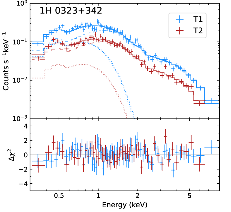
Figure 10: Stacked spectra and their best-fit models (upper panel) of 1H 0323+342 at “T1” (blue) and “T2” (red). The best-fit model, the power-law component and the blackbody component, are represented by solid, dashed and dotted lines, respectively. The residuals of the model fit to the spectra are shown in the lower panel.

For PKS 1502+036, the X-ray light curve does not show any visually obvious ‘peak’ or ‘valley’. So we do not choose such continuous periods as the high or low flux state. The spectra for stacking are selected only based on $f_{\rm soft}$ and $\alpha_{\rm ox}$, and each stacked spectrum has photon counts of $\sim 200$. For PKS 2004-447, there is neither a visually obvious ‘peak’/‘valley’ period nor a correlation between $\alpha_{\rm ox}$ and the X-ray flux. The spectra are only selected based on $f_{\rm soft}$ and each stacked spectrum has photon counts of $\sim 300$. A single power-law model with a Galactic neutral hydrogen absorption is adopted to fit the stacked spectra of PKS 1502+036 and PKS 2004-447, and the best-fit parameters are summarized in Table LABEL:tab:stacked1502 and LABEL:tab:stacked2004, respectively. For the other three sources in the sample, no spectral stacking is performed, since they were observed only a few times.

Table 4: Results of 1H 0323+342 blackbody+power law spectral fit to the stacked spectra

State	$\Gamma$	$kT$	$F_{\rm bb}$	$F_{\rm pl}$	$R$	$\chi^{2}$/dof
T1	1.74${}^{+0.06}_{-0.06}$	160${}^{+9}_{-9}$	43.9${}^{+3.2}_{-3.2}$	98.2${}^{+4.2}_{-4.1}$	44.8%	58.8/64
T2	1.85${}^{+0.07}_{-0.07}$	162${}^{+17}_{-18}$	9.8${}^{+1.3}_{-1.3}$	43.3${}^{+1.8}_{-1.7}$	22.7%	50.3/52
High flux	1.89${}^{+0.07}_{-0.07}$	150${}^{+13}_{-14}$	52.3${}^{+6.1}_{-6.0}$	182.3${}^{+8.3}_{-8.0}$	28.7%	54.3/53
Low flux	1.75${}^{+0.06}_{-0.06}$	170${}^{+40}_{-38}$	4.0${}^{+1.1}_{-1.1}$	41.5${}^{+1.4}_{-1.3}$	9.7%	75.7/60
Flat $\alpha_{\rm ox}$	1.88${}^{+0.06}_{-0.06}$	151${}^{+13}_{-14}$	47.8${}^{+5.6}_{-5.6}$	179.6${}^{+7.5}_{-7.3}$	26.6%	44.2/57
Steep $\alpha_{\rm ox}$	1.68${}^{+0.06}_{-0.06}$	171${}^{+15}_{-16}$	9.2${}^{+1.1}_{-1.1}$	41.3${}^{+1.4}_{-1.4}$	22.3%	66.5/62

Notes. A Galactic absorption of column density of $N^{\rm Gal}_{\rm H}=1.17\times 10^{21}\rm\,cm^{-2}$ is always included during the fitting. Column 2: Photon index. Column 3: Black body temperature in units of eV. Column 4: Flux of the black body component in the band 0.3–2 keV in units of $10^{-13}$ $\rm erg\,s^{-1}cm^{-2}$. Column 5: Flux of power law component in the band 0.3–2 keV in units of $10^{-13}$ $\rm erg\,s^{-1}cm^{-2}$. Column 6: Flux ratio of black body to power law in the band 0.3–2 keV. Column 7: $\chi^{2}$ and the degrees of freedom.