Direct Integral Pseudospectral and Integral Spectral Methods for Solving a Class of Infinite Horizon Optimal Output Feedback Control Problems Using Rational and Exponential Gegenbauer Polynomials

Abstract

This study is concerned with the numerical solution of a class of infinite-horizon linear regulation problems with state equality constraints and output feedback control. We propose two numerical methods to convert the optimal control problem into nonlinear programming problems (NLPs) using collocations in a semi-infinite domain based on rational Gegenbauer (RG) and exponential Gegenbauer (EG) basis functions. We introduce new properties of these basis functions and derive their quadratures and associated truncation errors. A rigorous stability analysis of the RG and EG interpolations is also presented. The effects of various parameters on the accuracy and efficiency of the proposed methods are investigated. The performance of the developed integral spectral method is demonstrated using two benchmark test problems related to a simple model of a divert control system and the lateral dynamics of an F-16 aircraft. Comparisons of the results of the current study with available numerical solutions show that the developed numerical scheme is efficient and exhibits faster convergence rates and higher accuracy.

1 Introduction

Infinite-horizon optimal control problems (IHOCs) of continuous-time linear systems with linear state equality constraints and output feedback control arise in systems with input equality constraints, particularly when the actuator dynamics are also considered in the problem so that the actuator outputs are augmented to the plant state vector. Typical examples of these systems include divert control system (DCS) models and the lateral dynamics of an F-16 aircraft. Only a few studies have appeared in the literature to solve such problems. An early attempt to solve the IHOCs of continuous-time linear systems with state equality constraints occurred in [1], where various existence conditions for constraining state feedback control were found before determining the optimal feedback gain via reduction of the control input space dimension. Cha et al. [2] extended this study to cover problems with output feedback by following the same approach presented earlier in [1]. However, a major drawback of the latter approach is the need to derive and solve a sophisticated system of optimal gain design equations for constrainable output feedback gains, which require either finding the optimal form of a non-unique basis matrix or fixing a basis matrix a priori before finding the optimal gain and then comparing the effect of the various basis matrices on the performance of the controller via numerical simulations.

In this study, we present the TG-IPS and TG-IS methods: Direct integral pseudospectral (IPS) and integral spectral (IS) methods based on rational Gegenbauer (RG) and exponential Gegenbauer (EG) functions for solving IHOCs of continuous-time linear systems with linear state equality constraints and output feedback control. Both methods overcome the drawbacks of the method of Ko and Bitmead [1] and Cha et al. [2] by directly converting the integral form of the problem into an NLP via efficient collocation on the original semi-infinite domain based on RG and EG functions, which we collectively refer to as transformed Gegenbauer (TG) functions. All integrals included in the problem in its integral form are approximated using novel and highly accurate quadratures based on TG functions. To guarantee the convergence of the proposed methods, we derive the parameter ranges over which the TG-based interpolation/collocation is stable through rigorous interpolation/collocation stability analysis. We later show that the TG-IS method is superior to the TG-IPS method in terms of computational complexity. Because the performance of both methods may vary considerably with the parameters used, a significant part of our study is devoted to deriving a crucial rule of thumb that provides a useful means to optimize the performance of the proposed methods by determining the optimal ranges of the collocation mesh size, Gegenbauer index, and the mapping scaling parameter associated with the TG basis functions. While TG functions were applied earlier in several works, cf. [3, 4, 5, 6] to mention a few, their application for solving the problem under study has never been considered in the literature, to the best of our knowledge. Another important contribution of this study is the ability of the proposed TG-IS method to determine the approximate optimal state and control variables with exponential convergence rates directly in the original semi-infinite domain. In contrast, common early approaches for solving IHOCs aimed to solve this class of problems through transformation into finite-horizon optimal control problems by using certain parametric mappings and then collocating the latter using classical Legendre and Gegenbauer polynomials. While these approaches can converge exponentially to near-optimal approximations for a coarse collocation mesh grid size, they usually diverge as the number of collocation points grows large if the computations are carried out using floating-point arithmetic, and the discretization uses a single mesh grid, regardless of whether they are of the Gauss/Gauss-Radau type or equally spaced; cf. [7] and the references therein. The current methods do not suffer from this limitation, as they generally remain stable for large mesh grids and certain parameter ranges, as we will demonstrate later in Section 7 and B. For a comprehensive review of IPS and IS methods, the reader may consult [7, 8, 9, 10, 11, 12, 13], and the references therein.

The remainder of this paper is organized as follows. In Section 2, we present some mathematical notations to be used later in this study. The problem under study is described in Section 3. The proposed TG-IPS and TG-IS methods are presented in Sections 4 and 5. Section 6 provides an error analysis of the TG quadrature derived in Section 4. Section 7 presents extensive numerical simulations to assess the performance of the TG quadratures and the proposed TG-IS method. Section 8 provides some concluding remarks followed by a future work in Section 9. A provides some properties of RG and EG functions and their associated Gaussian quadratures. Finally, B presents a rigorous stability study of TG interpolation/collocation.

2 Preliminary Notations

The following notations are used throughout this study to simplify the mathematical formulas. Most of these notations appeared recently in [14, 15, 16]; however, we present them here together with some new notations to keep the paper as self-explanatory as possible.

Logical and Relational Symbols. The symbols $\forall,\,\forall_{\mkern-6.0mua}\,,\,\forall_{\mkern-6.0mue}\,$, and $\,\forall_{\mkern-6.0mus}\,$ stand for the phrases “for all,” “for any,” “for each,” and “for some,” in respective order.  $<$$\sim$  and  $\leq$$\sim$  mean the statements “asymptotically less than” and “asymptotically less than or equal to,” respectively.
Set and List Notations. $\mathbb{R},\mathbb{R}_{\hbox to0.0pt{\raisebox{1.12778pt}{\textcolor{black}{\rule{2.8pt}{0.5pt}}}\hss}0}$, and $\mathbb{R}_{0}^{+}$ are the sets of real, non-zero real, and nonnegative real numbers, respectively. $\mathbb{Z},\mathbb{Z}_{0}^{+}$, and $\mathrel{\mathop{\mathbb{Z}^{+}}\limits^{\vbox to0.0pt{\kern-2.0pt\hbox{$\scriptstyle\rightarrow$}\vss}}}$ are the sets of integer, nonnegative integer, and sufficiently large positive integer numbers, respectively. We define also the two sets $\mathrel{\mathop{\mathbb{R}}\limits^{\vbox to0.0pt{\kern-2.0pt\hbox{$\scriptstyle\rightarrow$}\vss}}}_{-1/2}=\{x\in\mathbb{R}:x>-1/2\}$ and $\mathbb{R}_{-1/2}^{-}=\{x\in\mathbb{R}:-1/2<x<0\}$. $\mathfrak{F}$ denotes the set of all real-valued functions. $\operatorname{span}\mathbb{S}$ stands for the set of all linear combinations of the vectors/functions in the set $\mathbb{S}$. The notations $i$:$j$:$k$ or $i(j)k$ indicate a list of numbers from $i$ to $k$ with increment $j$ between numbers, unless the increment equals one where we use the simplified notation $i$:$k$. The list of symbols $y_{1},y_{2},\ldots,y_{n}$ is denoted by $\left.y_{i}\right|_{i=1:n}$ or simply $y_{1:n}$, and their set is represented by $\{y_{1:n}\}\,\,\forall_{\mkern-6.0mua}\,n\in\mathbb{Z}^{+}$. This notation is further extended to any symbol with multiple subscripts; for example, $y_{1:m,0:n}$ stands for the list of symbols $y_{1,0},y_{1,1},\ldots,y_{1,n},y_{2,0},\ldots,y_{2,n},\ldots,y_{m,n}$. We define $\mathbb{J}_{n}=\{0$:$n\}$ and $\mathbb{N}_{N}=\{1$:$N\}\,\,\forall_{\mkern-6.0mua}\,n\in\mathbb{Z}_{0}^{+},N\in\mathbb{Z}^{+}$. $\mathbb{G}_{n}^{\alpha}=\left\{x_{n,0:n}^{\alpha}\right\}$ is the zeros set of the $(n+1)$st-degree Gegenbauer polynomial with index $\alpha\in\,\mathrel{\mathop{\mathbb{R}}\limits^{\vbox to0.0pt{\kern-2.0pt\hbox{$\scriptstyle\rightarrow$}\vss}}}_{-1/2}$ (aka the Gegenbauer-Gauss (GG) points set) $\,\forall_{\mkern-6.0mua}\,n\in\mathbb{Z}^{+}$. Finally, the specific interval $[0,c]$ is denoted by $\mathbf{\Omega}_{c}\,\forall c>0$. For example, $[0,x_{n,j}^{\alpha}]$ is denoted by ${\mathbf{\Omega}_{x_{n,j}^{\alpha}}}$; moreover, ${\mathbf{\Omega}_{x_{n,0:n}^{\alpha}}}$ stands for the list of intervals ${\mathbf{\Omega}_{x_{n,0}^{\alpha}}},{\mathbf{\Omega}_{x_{n,1}^{\alpha}}},\ldots,{\mathbf{\Omega}_{x_{n,n}^{\alpha}}}$.
Function Notations. $\delta_{m,n}$ is the usual Kronecker delta function of variables $m$ and $n$. $\Gamma$ and $\digamma$ denote the Gamma function and its logarithmic derivative. $H_{x}$ is the Harmonic number real-continuation function defined by $H_{x}=\digamma(x)+\gamma_{em}\,\forall x\in\mathbb{R}:H_{n}$ is the usual Harmonic number function $\forall n\in\mathbb{Z}^{+}$ and $\gamma_{em}$ is the Euler-Mascheroni constant defined by

$$\gamma_{em}=\mathop{\lim}\limits_{n\to\infty}\left({-\ln n+\sum\limits_{k=1}^{n}{\frac{1}{k}}}\right)\approx 0.577216,$$

rounded to six decimal digits. $G_{n}^{\alpha}(x)$ is the $n$th-degree Gegenbauer polynomial with index $\alpha\in\,\mathrel{\mathop{\mathbb{R}}\limits^{\vbox to0.0pt{\kern-2.0pt\hbox{$\scriptstyle\rightarrow$}\vss}}}_{-1/2}$ such that $G_{n}^{\alpha}(1)=1\,\forall n\in\mathbb{Z}_{0}^{+}$. For convenience, we shall denote $h\left(x_{n,j}^{\alpha}\right)$ and $h\left({}_{i}^{L}t_{n,j}^{\alpha}\right)$ by $h_{n,j}^{\alpha}$ and $h_{i,n,j}^{\alpha,L}\,\,\forall_{\mkern-6.0mua}\,h\in\mathfrak{F},{}_{i}^{L}t_{n}^{\alpha}\in\mathbb{R}_{0}^{+}:(n,j,i,L)\in\mathbb{Z}_{0}^{+}\times\mathbb{J}_{n}\times\mathbb{N}_{2}\times\mathbb{Z}^{+}$, unless stated otherwise.
Integral Notations. We denote $\int_{0}^{b}{h(t)\,dt}$ and $\int_{a}^{b}{h(t)\,dt}$ by $\mathcal{I}_{b}^{(t)}h$ and $\mathcal{I}_{a,b}^{(t)}h$, respectively, $\,\forall_{\mkern-6.0mua}\,h\in\mathfrak{F},\{a,b\}\subset\mathbb{R}$. $\mathcal{I}_{\mathbf{\Omega}}^{(x)}{h}$ means $\int_{\mathbf{\Omega}}{h(x)\,dx}\,\,\forall_{\mkern-6.0mua}\,$ interval $\mathbf{\Omega}\subseteq\mathbb{R}$. If the integrand function $h$ is to be evaluated at any other expression of $x$, say $u(x)$, we express $\int_{0}^{b}{h(u(x))\,dx}$ and $\int_{a}^{b}{h(u(x))\,dx}$ with a stroke through the square brackets as $\mathcal{I}_{b}^{(x)}h\hbox to0.0pt{\raisebox{1.875pt}{\textcolor{black}{\rule{2.22223pt}{0.5pt}}}\hss}[u(x)\hbox to0.0pt{\raisebox{1.875pt}{\textcolor{black}{\hskip 0.85358pt\rule{1.94443pt}{0.75pt}}}\hss}]$ and $\mathcal{I}_{a,b}^{(x)}h\hbox to0.0pt{\raisebox{1.875pt}{\textcolor{black}{\rule{2.22223pt}{0.5pt}}}\hss}[u(x)\hbox to0.0pt{\raisebox{1.875pt}{\textcolor{black}{\hskip 0.85358pt\rule{1.94443pt}{0.75pt}}}\hss}]$ in respective order. Here, the strike-through notation is introduced to indicate that $h$ is a function of $u(x)$ and the integration is to be evaluated under this assumption; this is useful if we wish to avoid evaluating the integral of $h$ first and then multiply the result by $u(x)$.
Space, Norm, and Inner Product Notations. $\text{Def}\left(\mathbf{\Omega}\right)$ is the space of functions defined on the set $\mathbf{\Omega}$. $\,\forall_{\mkern-6.0mua}\,\mathbf{\Omega}\subseteq\mathbb{R},L^{p}({\mathbf{\Omega}})$ is the Banach space of measurable functions $u\in\text{Def}\left(\mathbf{\Omega}\right)$ with the norm ${\left\|u\right\|_{{L^{p}_{w}(\mathbf{\Omega})}}}={\left[\mathcal{I}_{\mathbf{\Omega}}^{(x)}{\left({|u|}^{p}\,w\right)}\right]^{1/p}}<\infty\,\forall p\geq 1$, where $w$ is some weight function in the usual sense; the subscript $w$ in ${L^{p}_{w}(\mathbf{\Omega})}$ is omitted when $w(x)=1\,\forall x\in\mathbf{\Omega}$. For $p=\infty$, the space ${L^{\infty}(\mathbf{\Omega})}$ is the space of bounded measurable functions with the norm $\left\|u\right\|_{L^{\infty}(\mathbf{\Omega})}=\sup_{\bm{x}\in\mathbf{\Omega}}{\left|u(\bm{x})\right|}\,\,\forall_{\mkern-6.0mua}\,\mathbf{\Omega}\subseteq\mathbb{R}^{n}$. We denote by $(u,v)_{w}$ the inner product of the space $L^{2}_{w}(\mathbf{\Omega})$ such that $(u,v)_{w}=\mathcal{I}^{(x)}_{\mathbf{\Omega}}{(uvw)}\,\,\forall_{\mkern-6.0mua}\,\{u,v\}\subset\text{Def}\left(\mathbf{\Omega}\right)$. We define the Sobolev space $H^{m}_{w}(\mathbf{\Omega})=\{u:u^{(k)}\in L_{w}^{2}(\mathbf{\Omega})\,\forall k\in\mathbb{J}_{m}\}$. Finally, $\left\|\mathcal{E}\right\|_{\max}$ denotes the largest element of $\mathcal{E}$ in magnitude $\,\forall_{\mkern-6.0mua}\,n$-dimensional array of real numbers $\mathcal{E}$.
Vector Notations. $\forall\{i,n,L\}\subset\mathbb{Z}^{+}$, we shall use the shorthand notations $\bm{x}_{n}^{\alpha}\left(\text{or }{x_{0:n}^{\alpha}}^{\top}\right)$ and ${}_{i}^{L}\bm{t}_{n}^{\alpha}\left(\text{or }{{}_{i}^{L}t_{0:n}^{\alpha}}^{\top}\right)$ to stand for the column vectors $[x_{n,0}^{\alpha},x_{n,1}^{\alpha},\ldots,x_{n,n}^{\alpha}]^{\top}$ and $[{}_{i}^{L}t_{n,0}^{\alpha},{}_{i}^{L}t_{n,1}^{\alpha},\ldots,{}_{i}^{L}t_{n,n}^{\alpha}]^{\top}$ in respective order. Moreover, $h_{n,0:n}^{\alpha},h_{i,n,0:n}^{\alpha,L}$, and $c^{0:n}$ denote $[h_{n,0}^{\alpha},h_{n,1}^{\alpha},\ldots,h_{n,n}^{\alpha}]^{\top},[h_{i,n,0}^{\alpha,L},h_{i,n,1}^{\alpha,L},\ldots,h_{i,n,n}^{\alpha,L}]^{\top}$, and the $n$th-dimensional row vector $[c^{0},c^{1},\ldots,c^{n}]$ $\,\forall_{\mkern-6.0mua}\,c\in\mathbb{R}_{\hbox to0.0pt{\raisebox{1.12778pt}{\textcolor{black}{\rule{2.8pt}{0.5pt}}}\hss}0}$, respectively. In general, $\,\forall_{\mkern-6.0mua}\,h\in\mathfrak{F}$ and vector $\bm{y}$ whose $i$th-element is $y_{i}\in\mathbb{R}$, the notation $h(\bm{y})$ stands for a vector of the same size and structure of $\bm{y}$ such that $h(y_{i})$ is the $i$th element of $h(\bm{y})$. Moreover, by $\bm{h}(\bm{y})$ (or $h_{1:m}\hbox to0.0pt{\raisebox{1.875pt}{\textcolor{black}{\rule{2.22223pt}{0.5pt}}}\hss}[\bm{y}\hbox to0.0pt{\raisebox{1.875pt}{\textcolor{black}{\hskip 0.85358pt\rule{1.94443pt}{0.75pt}}}\hss}]$) with a stroke through the square brackets, we mean $[h_{1}(\bm{y}),\ldots,h_{m}(\bm{y})]^{\top}\,\,\forall_{\mkern-6.0mua}\,m$-dimensional column vector function $\bm{h}$, with the realization that the definition of each array $h_{i}(\bm{y})$ follows the former notation rule $\,\forall_{\mkern-6.0mue}\,i$. We adopt the notation $\mathcal{I}_{{\bm{t}_{n}}}^{(t)}h$ to denote the $(n+1)$st-dimensional column vector $\left[{\mathcal{I}_{{t_{n,0}}}^{(t)}h,\mathcal{I}_{{t_{n,1}}}^{(t)}h,\ldots,\mathcal{I}_{{t_{n,n}}}^{(t)}h}\right]^{\top}$. Furthermore, we write $\mathcal{I}_{{\bm{t}_{n}}}^{(t)}\bm{h}$ to denote the $(n+1)\times m$ matrix $\left[\mathcal{I}_{{t_{n,0}}}^{(t)}\bm{h},\mathcal{I}_{{t_{n,1}}}^{(t)}\bm{h},\ldots,\right.$ $\left.\mathcal{I}_{{t_{n,n}}}^{(t)}\bm{h}\right]^{\top}\,\,\forall_{\mkern-6.0mua}\,m$-dimensional vector function $\bm{h}$.
Matrix Notations and Operations. $\mathbf{O}_{n},\mathbf{1}_{n}$, and $\mathbf{I}_{n}$ stand for the zero, all ones, and the identity matrices of size $n$. By $[\mathbf{A}\,;\mathbf{B}]$ we mean the usual vertical matrix concatenation of $\mathbf{A}$ and $\mathbf{B}\,\,\forall_{\mkern-6.0mua}\,$ two matrices $\mathbf{A}$ and $\mathbf{B}$ having the same number of columns. For a two-dimensional matrix $\mathbf{C}$, the notation $\mathbf{C}_{\hbox to0.0pt{\raisebox{1.12778pt}{\textcolor{black}{\rule{2.8pt}{0.5pt}}}\hss}0}$ stands for the matrix obtained by deleting the zeroth-row of $\mathbf{C}$. $\mathbf{C}_{n,m}$ indicates that $\mathbf{C}$ is a rectangular matrix of size $n\times m$. The notations $\mathbf{A}^{\top}$ (or $\text{trp}\left(\mathbf{A}\right)$), $\text{vec}\left(\mathbf{A}\right)$, and $\text{siz}\left(\mathbf{A}\right)$ denote the transpose, the vectorization, and the size of a matrix $\mathbf{A}$, respectively. $\max(\mathbf{A})$ denotes the row vector containing the columns’ maximum values of a matrix $\mathbf{A}$. $\text{resh}_{m,n}\left(\mathbf{A}\right)$ and $\text{resh}_{n}\left(\mathbf{A}\right)$ are the matrices obtained by reshaping $\mathbf{A}$ into an $m$-by-$n$ matrix and a square matrix of size $n$, respectively while preserving their column-wise ordering from $\mathbf{A}$. $\text{diag}\left(\bm{v}\right)$ denotes a square diagonal matrix with the elements of vector $\bm{v}$ on the main diagonal. $\odot,\oslash$, and $\otimes$ denote the usual Hadamard product and division, and Kronecker product of matrices in respective order. We adopt the notation $\mathbf{A}_{(r)}$ to denote the $r$-times Hadamard product $\mathbf{A}\circ\mathbf{A}\circ\ldots\circ\mathbf{A}\,\,\forall_{\mkern-6.0mua}\,$ array $\mathbf{A}$. We assume that the Hadamard arithmetic operations have a lower order of precedence over the conventional matrix arithmetic operations. For convenience, a vector is represented in print by a bold italicized symbol while a two-dimensional matrix is represented by a bold symbol, except for a row vector whose elements form a certain row of a matrix where we represent it in bold symbol as stated earlier. For example, $\bm{\mathit{1}}_{n}$ and $\bm{\mathit{0}}_{n}$ denote the $n$-dimensional all ones- and zeros- column vectors, while $\mathbf{1}_{n}$ and $\mathbf{O}_{n}$ denote the all ones- and zeros- matrices of size $n$, respectively. Finally, the symbols $\bm{u}^{\div}$ and $\bm{v}^{\div}$ stand for $\bm{\mathit{1}}_{n}^{\top}\oslash\bm{u}$ and $\bm{\mathit{1}}_{n}\oslash\bm{v}\,\forall\{\bm{u}^{\top},\bm{v}\}\subset\mathbb{R}^{n}$.

3 The Problem Statement

Consider the following time-invariant linear control system of ordinary differential equations described by

$$\dot{\bm{x}}(t) =\mathbf{A}\bm{x}(t)+\mathbf{B}\,\bm{u}(t),$$ (3.1a)

$$\bm{y}(t) =\mathbf{C}\bm{x}(t),$$ (3.1b)

with design state constraints

$$\mathbf{D}^{\top}\bm{x}(t)=\bm{\mathit{0}},$$ (3.1c)

$$\forall t\in\mathbb{R}_{0}^{+} \bm{x}(t)=x_{1:n_{x}}\hbox to0.0pt{\raisebox{1.875pt}{\textcolor{black}{\rule{2.22223pt}{0.5pt}}}\hss}[t\hbox to0.0pt{\raisebox{1.875pt}{\textcolor{black}{\hskip 0.85358pt\rule{1.94443pt}{0.75pt}}}\hss}],\bm{u}(t)=u_{1:n_{u}}\hbox to0.0pt{\raisebox{1.875pt}{\textcolor{black}{\rule{2.22223pt}{0.5pt}}}\hss}[t\hbox to0.0pt{\raisebox{1.875pt}{\textcolor{black}{\hskip 0.85358pt\rule{1.94443pt}{0.75pt}}}\hss}],\bm{y}(t)=y_{1:n_{y}}\hbox to0.0pt{\raisebox{1.875pt}{\textcolor{black}{\rule{2.22223pt}{0.5pt}}}\hss}[t\hbox to0.0pt{\raisebox{1.875pt}{\textcolor{black}{\hskip 0.85358pt\rule{1.94443pt}{0.75pt}}}\hss}],\mathbf{A}\in\mathbb{R}^{n_{x}\times n_{x}},\mathbf{B}\in\mathbb{R}^{n_{x}\times n_{u}},\mathbf{C}\in\mathbb{R}^{n_{y}\times n_{x}} \mathbf{D}\in\mathbb{R}^{n_{x}\times c_{1}}\,\,\forall_{\mkern-6.0mus}\,\{n_{x},n_{u},n_{y},c_{1}\}\subset\mathbb{Z}^{+}$$, where , and . The problem is to find the optimal output feedback control law

$$\bm{u}(t)=-\mathbf{K}\bm{y}(t)\quad\,\forall_{\mkern-6.0mus}\,\mathbf{K}\in\mathbb{R}^{n_{u}\times n_{y}},$$ (3.1d)

the corresponding optimal state trajectory $$\bm{x} \bm{y} \mathbb{R}_{0}^{+}$$, and the output feedback on the semi-infinite domain that satisfy Eqs. (3.1a)–(3.1c) while minimizing the functional

$$J=\frac{1}{2}\mathcal{I}_{\mathbb{R}_{0}^{+}}^{(t)}{\left(\bm{x}^{\top}\mathbf{Q}\,\bm{x}+\bm{u}^{\top}\mathbf{R}\,\bm{u}\right)},$$ (3.1e)

where $\mathbf{Q}\in\mathbb{R}^{n_{x}\times n_{x}}$ and $\mathbf{R}\in\mathbb{R}^{n_{u}\times n_{u}}$ are symmetric positive semi-definite matrices. We refer to the OC problem described by Eqs. (3.1a)–(3.1e) by Problem $\mathscr{A}$.

4 The TG-IPS Method

In this section, we describe an IPS method for solving Problem $\mathscr{A}$ based on TG collocation at the TGG points. We show later how to boost the performance of this method in Section 5. We highly recommend reading A and B first before reading this section to learn more about the properties of the basis functions and their associated Gaussian quadratures employed in our methods, in addition to the stability characteristics associated with TG interpolation/collocation, which provide useful insight on the parameters ranges of values suitable to run our methods while maintaining highly accurate, robust, and efficient solutions to the mathematical problem.

To approximate the system dynamics equations and constraints (3.1a)– (3.1c) using TG-based collocation, we first show how to calculate the quadrature of a function $f\in\text{Def}\left(\mathbb{R}_{0}^{+}\right)$ on the successive integrals $\mathbf{\Omega}_{{}_{i}^{L}t_{n,0:n}^{\alpha}}$ using the TGG quadrature. To this end, let ${}_{i}^{L}\bm{E}_{n}^{\alpha}=e^{-{}_{i}^{L}\bm{t}^{\alpha}_{n}}$ and ${}_{i}{\bm{W}^{\alpha,L}_{n}}=\bm{\varpi}_{n}^{\alpha}\oslash w^{\alpha,L}_{i}\left({}_{i}^{L}{\bm{t}_{n}^{\alpha}}^{\top}\right)\,\forall i\in\mathbb{N}_{2}$. Using the following change of variables

$$t={}_{i}^{L}t^{\alpha}_{n,j}\,e^{-z},$$ (4.1)

we can write

$$\mathcal{I}_{{}_{i}^{L}t_{n,j}^{\alpha}}^{(t)}{f}={}_{i}^{L}t_{n,j}^{\alpha}\,\mathcal{I}_{\mathbb{R}_{0}^{+}}^{(z)}{\left(e^{-z}f\hbox to0.0pt{\raisebox{1.875pt}{\textcolor{black}{\rule{2.22223pt}{0.5pt}}}\hss}[{}_{i}^{L}t^{\alpha}_{n,j}\,e^{-z}\hbox to0.0pt{\raisebox{1.875pt}{\textcolor{black}{\hskip 0.85358pt\rule{1.94443pt}{0.75pt}}}\hss}]\right)}\quad\forall j\in\mathbb{J}_{n},$$ (4.2)

which can be approximated by Lemma A.1 as follows:

$$\mathcal{I}^{(t)}_{{}_{i}^{L}t^{\alpha}_{n,j}}{f}\approx{}_{i}\mathcal{Q}_{n,j}^{\alpha,L}={}_{i}^{L}t^{\alpha}_{n,j}\left[{}_{i}^{L}\bm{P}^{\alpha}_{n}\,f\left({}_{i}^{L}t^{\alpha}_{n,j}\,{}_{i}^{L}\bm{E}_{n}^{\alpha}\right)\right],$$ (4.3)

where ${}_{i}^{L}\bm{P}^{\alpha}_{n}={}_{i}{\bm{W}^{\alpha,L}_{n}}\odot{}_{i}^{L}{\bm{E}_{n}^{\alpha}}^{\top}\,\forall i\in\mathbb{N}_{2}$ are the RG and EG integration vectors, respectively, which are collectively called “the TG integration vector.” Formula (4.3) provides a means to compute the quadrature of $f\in\text{Def}\left(\mathbb{R}_{0}^{+}\right)$ on the successive integrals $\mathbf{\Omega}_{{}_{i}^{L}t_{n,0:n}^{\alpha}}$ using the TGG quadratures of the auxiliary functions ${}_{i}^{L}g_{n,j}^{\alpha}\in\text{Def}\left(\mathbb{R}_{0}^{+}\right)$:

$$\quad{}_{i}^{L}g_{n,j}^{\alpha}(t)={}_{i}^{L}t_{n,j}^{\alpha}\,\frac{e^{-t}f\left({}_{i}^{L}t^{\alpha}_{n,j}\,e^{-t}\right)}{w_{i}^{\alpha,L}(t)}\quad\forall(i,n,\alpha,L)\in\mathbb{N}_{2}\times\mathbb{Z}_{0}^{+}\times\mathrel{\mathop{\mathbb{R}}\limits^{\vbox to0.0pt{\kern-2.0pt\hbox{$\scriptstyle\rightarrow$}\vss}}}_{-1/2}\times\mathbb{R}^{+}.$$ (4.4)

Formula (4.3) can be further rewritten in the following matrix notation:

$$\mathcal{I}^{(t)}_{{}_{i}^{L}\bm{t}^{\alpha}_{n}}{f}\approx{}_{i}\mathbfcal{Q}_{n}^{\alpha,L}={}_{i}^{L}\bm{t}^{\alpha}_{n}\odot\left[f\left({}_{i}^{L}\bm{\xi}^{\alpha}_{n}\right)\,{}_{i}^{L}{\bm{P}^{\alpha}_{n}}^{\top}\right],$$ (4.5)

where ${}_{i}^{L}\bm{\xi}^{\alpha}_{n}={}_{i}^{L}\bm{t}^{\alpha}_{n}\otimes{}_{i}^{L}{\bm{E}_{n}^{\alpha}}^{\top}$. We refer to ${}_{i}\mathcal{Q}_{n,j}^{\alpha,L}\,\forall i=1$:$2$ by the RG and EG quadratures associated with the TGG node ${}_{i}^{L}t_{n,j}^{\alpha}\,\,\forall_{\mkern-6.0mue}\,j\in\mathbb{J}_{n}$, respectively, or collectively by “the TG quadrature.”

Now, let $\mathbf{X}=x_{1:n_{x}}^{\top}\hbox to0.0pt{\raisebox{1.875pt}{\textcolor{black}{\rule{2.22223pt}{0.5pt}}}\hss}[{}_{i}^{L}\bm{t}_{n}^{\alpha}\hbox to0.0pt{\raisebox{1.875pt}{\textcolor{black}{\hskip 0.85358pt\rule{1.94443pt}{0.75pt}}}\hss}],\mathbf{Y}=y_{1:n_{y}}^{\top}\hbox to0.0pt{\raisebox{1.875pt}{\textcolor{black}{\rule{2.22223pt}{0.5pt}}}\hss}[{}_{i}^{L}\bm{t}_{n}^{\alpha}\hbox to0.0pt{\raisebox{1.875pt}{\textcolor{black}{\hskip 0.85358pt\rule{1.94443pt}{0.75pt}}}\hss}],\mathbf{U}=u_{1:n_{u}}^{\top}\hbox to0.0pt{\raisebox{1.875pt}{\textcolor{black}{\rule{2.22223pt}{0.5pt}}}\hss}[{}_{i}^{L}\bm{t}_{n}^{\alpha}\hbox to0.0pt{\raisebox{1.875pt}{\textcolor{black}{\hskip 0.85358pt\rule{1.94443pt}{0.75pt}}}\hss}]$, and ${}_{i}^{L}{\hat{\mathbf{P}}^{\alpha}_{n}}={}_{i}^{L}\bm{P}^{\alpha}_{n}\otimes\mathbf{I}_{n+1}$. To take advantage later of the well-conditioning of numerical integration operators during the collocation phase, we initially rewrite (3.1a) in its integral formulation as follows:

$$\bm{x}(t)=\mathbf{A}\mathcal{I}^{(z)}_{t}{\bm{x}}+\mathbf{B}\mathcal{I}^{(z)}_{t}{\bm{u}}+\bm{x}(0)\quad\forall t\in\mathbb{R}_{0}^{+}.$$ (4.6)

The TG quadrature (4.5) immediately yields

$$\mathcal{I}_{{{}_{i}^{L}\bm{t}_{n}^{\alpha}}}^{(z)}(\mathbf{A}\bm{x})\approx\left(\bm{\mathit{1}}_{n_{x}}^{\top}\otimes{}_{i}^{L}\bm{t}^{\alpha}_{n}\right)\odot\left[\mathbf{X}_{\bm{\xi}}\left(\mathbf{I}_{n_{x}}\otimes\,{}_{i}^{L}{\bm{P}_{n}^{\alpha}}^{\top}\right)\mathbf{A}^{\top}\right],$$ (4.7a)

and

$$\mathcal{I}_{{{}_{i}^{L}\bm{t}_{n}^{\alpha}}}^{(z)}(\mathbf{B}\bm{u})\approx\left[\left(\bm{\mathit{1}}_{n_{u}}^{\top}\otimes{}_{i}^{L}\bm{t}^{\alpha}_{n}\right)\odot\mathbf{U}_{\bm{\xi}}\left(\mathbf{I}_{n_{u}}\otimes\,{}_{i}^{L}{\bm{P}_{n}^{\alpha}}^{\top}\right)\right]\mathbf{B}^{\top},$$ (4.7b)

where $\mathbf{X}_{\bm{\xi}}=x_{1:n_{x}}^{\top}\hbox to0.0pt{\raisebox{1.875pt}{\textcolor{black}{\rule{2.22223pt}{0.5pt}}}\hss}[{}_{i}^{L}\bm{\xi}_{n}^{\alpha}\hbox to0.0pt{\raisebox{1.875pt}{\textcolor{black}{\hskip 0.85358pt\rule{1.94443pt}{0.75pt}}}\hss}]$ and $\mathbf{U}_{\bm{\xi}}=u_{1:n_{u}}^{\top}\hbox to0.0pt{\raisebox{1.875pt}{\textcolor{black}{\rule{2.22223pt}{0.5pt}}}\hss}[{}_{i}^{L}\bm{\xi}_{n}^{\alpha}\hbox to0.0pt{\raisebox{1.875pt}{\textcolor{black}{\hskip 0.85358pt\rule{1.94443pt}{0.75pt}}}\hss}]$. Therefore, the collocation of Eq. (4.6) at the TGG nodes gives

$$\bm{x}\left({}_{i}^{L}\bm{t}^{\alpha}_{n}\right) \approx\text{vec}\left[\left(\bm{\mathit{1}}_{n_{x}}^{\top}\otimes{}_{i}^{L}\bm{t}^{\alpha}_{n}\right)\odot\mathbf{X}_{\bm{\xi}}\left(\mathbf{I}_{n_{x}}\otimes\,{}_{i}^{L}{\bm{P}_{n}^{\alpha}}^{\top}\right)\mathbf{A}^{\top}\right]+\text{vec}\left[\left(\bm{\mathit{1}}_{n_{u}}^{\top}\otimes{}_{i}^{L}\bm{t}^{\alpha}_{n}\right)\odot\mathbf{U}_{\bm{\xi}}\left(\mathbf{I}_{n_{u}}\otimes\,{}_{i}^{L}{\bm{P}_{n}^{\alpha}}^{\top}\right)\mathbf{B}^{\top}\right]+\bm{x}\left(0\right)\otimes{\bm{\mathit{1}}}_{n+1}$$

$$={}_{i}\bm{T}_{n,n_{x}}^{\alpha}\odot\left[\bm{\psi}_{A}\bm{x}\left({}_{i}^{L}\bm{\eta}_{n}^{\alpha}\right)\right]+\mathbf{B}_{n}\left[{}_{i}\bm{T}_{n,n_{u}}^{\alpha}\odot{}_{i}^{L}{\tilde{\mathbf{P}}_{n,n_{u}}^{\alpha}}\,\bm{u}\left({}_{i}^{L}\bm{\eta}_{n}^{\alpha}\right)\right]+\bm{x}\left(0\right)\otimes{\bm{\mathit{1}}}_{n+1},$$ (4.8a)

where $${}_{i}\bm{T}_{n,m}^{\alpha}=\bm{\mathit{1}}_{m}\otimes{}_{i}^{L}\bm{t}^{\alpha}_{n}\,\forall m\in\mathbb{Z}^{+},\bm{\psi}_{A}=\mathbf{A}\otimes{}_{i}^{L}{\hat{\mathbf{P}}^{\alpha}_{n}},{}_{i}^{L}\bm{\eta}_{n}^{\alpha}={}_{i}^{L}\bm{E}_{n}^{\alpha}\otimes{}_{i}^{L}\bm{t}^{\alpha}_{n},\mathbf{B}_{n}=\mathbf{B}\otimes\mathbf{I}_{n+1} {}_{i}^{L}{\tilde{\mathbf{P}}_{n,n_{u}}^{\alpha}}=\mathbf{I}_{n_{u}}\otimes{}_{i}^{L}{\hat{\mathbf{P}}^{\alpha}_{n}}$$, and . The collocation of Eqs. (3.1b) and (3.1c) at the TGG nodes yield

$$\mathbf{Y} =\mathbf{X}\mathbf{C}^{\top},$$ (4.8b)

$$\mathbf{X}\mathbf{D} =\mathbf{O}_{n+1,c_{1}},$$ (4.8c)

respectively. We can readily approximate the performance index (3.1e) by using the TGG quadrature (A.14) to obtain

$$J\approx J_{n}=\frac{1}{2}\left({}_{i}{\bm{W}^{\alpha,L}_{n}}\,g_{0:n}\right),$$ (4.8d)

where $g_{j}=\bm{x}^{\top}\left({}_{i}^{L}t_{j}^{\alpha}\right)\mathbf{Q}\bm{x}\left({}_{i}^{L}t_{j}^{\alpha}\right)+\bm{u}^{\top}\left({}_{i}^{L}t_{j}^{\alpha}\right)\mathbf{R}\bm{u}\left({}_{i}^{L}t_{j}^{\alpha}\right)\,\forall j\in\mathbb{J}_{n}$. Problem $\mathscr{A}$ is now converted into an NLP in which the goal is to minimize the discrete cost functional (4.8d) subject to Constraints (4.8a) and (4.8c). We can solve the NLP using modern optimization methods for the optimal states and control variables, $\bm{x}^{*}$ and $\bm{u}^{*}$, at the TGG points, and the corresponding optimal output feedback variables can then be obtained by using Eq. (4.8b). Furthermore, the optimal output feedback gain $\mathbf{K}^{*}$ can be estimated by solving the following linear system of equations

$$\mathbf{K}^{*}\,{\mathbf{Y}^{*}}^{\top}=-{\mathbf{U}^{*}}^{\top},$$ (4.9)

for $\mathbf{K}^{*}$, where $\mathbf{Y}^{*}={y^{*}_{1:n_{y}}}^{\top}\;\hbox to0.0pt{\raisebox{1.875pt}{\textcolor{black}{\rule{2.22223pt}{0.5pt}}}\hss}[{}_{i}^{L}\bm{t}_{n}^{\alpha}\hbox to0.0pt{\raisebox{1.875pt}{\textcolor{black}{\hskip 0.85358pt\rule{1.94443pt}{0.75pt}}}\hss}]$ and $\mathbf{U}^{*}={u^{*}_{1:n_{u}}}^{\top}\;\hbox to0.0pt{\raisebox{1.875pt}{\textcolor{black}{\rule{2.22223pt}{0.5pt}}}\hss}[{}_{i}^{L}\bm{t}_{n}^{\alpha}\hbox to0.0pt{\raisebox{1.875pt}{\textcolor{black}{\hskip 0.85358pt\rule{1.94443pt}{0.75pt}}}\hss}]$. In the following section, we prescribe an alternative to the TG-IPS method that can significantly improve its computational performance in practice.

5 The TG-IS Method

A practical difficulty in solving the NLP obtained by the TG-IPS method arises from the need to estimate the optimal state and control variables at the additional mesh grid of points ${}_{i}^{L}\bm{\eta}_{n}^{\alpha}$ as well as the TGG points ${}_{i}^{L}\bm{t}_{n}^{\alpha}$ during the numerical optimization procedure. In particular, since $\text{siz}\left({}_{i}^{L}\bm{\eta}_{n}^{\alpha}\right)=\text{siz}^{2}\left({}_{i}^{L}\bm{t}_{n}^{\alpha}\right)$, the derived NLP has the dimension $(n+1)(n+2)(n_{x}+n_{u})$, which increases quadratically with the collocation mesh size. Therefore, the NLP may require a well-developed large-scale optimization method for large mesh grids. To overcome this difficulty, one approach is to solve the NLP in the TG spectral space by imposing the system dynamics equations and constraints at the TGG points using the TG modal expansions of the state and control variables in lieu of their nodal expansions and solve the converted NLP for the TG spectral coefficients. This procedure achieves a significant computational improvement by reducing the NLP dimensionality to only $(n+1)(n_{x}+n_{u})$, which grows linearly with the collocation mesh size. We describe this computationally attractive approach in the following.

Let $\mathbf{a}=\left[\bm{a}_{1};\ldots;\bm{a}_{n_{x}}\right]$ and $\mathbf{b}=\left[\bm{b}_{1};\ldots;\bm{b}_{n_{u}}\right]$ be the coefficients vectors of the TG collocants of the state and control variables such that $\bm{a}_{r}=a_{r,0:L_{x}}$ and $\bm{b}_{s}=b_{s,0:L_{u}}\,\forall r\in\mathbb{N}_{n_{x}},s\in\mathbb{N}_{n_{u}}$. Define also $\hat{\mathcal{G}}_{i,0:m}^{\alpha,L}\hbox to0.0pt{\raisebox{1.875pt}{\textcolor{black}{\rule{2.22223pt}{0.5pt}}}\hss}[t\hbox to0.0pt{\raisebox{1.875pt}{\textcolor{black}{\hskip 0.85358pt\rule{1.94443pt}{0.75pt}}}\hss}]=\text{trp}\left(\mathcal{G}_{i,0:m}^{\alpha,L}\hbox to0.0pt{\raisebox{1.875pt}{\textcolor{black}{\rule{2.22223pt}{0.5pt}}}\hss}[t\hbox to0.0pt{\raisebox{1.875pt}{\textcolor{black}{\hskip 0.85358pt\rule{1.94443pt}{0.75pt}}}\hss}]\right)\,\forall m\in\mathbb{Z}_{0}^{+}$. Then we can write the inverse discrete TG transform of the state and control variables at any time instance $t\in\mathbb{R}_{0}^{+}$ as follows:

$$\bm{x}(t) \approx\mathbf{a}\,\mathcal{G}_{i,0:L_{x}}^{\alpha,L}\hbox to0.0pt{\raisebox{1.875pt}{\textcolor{black}{\rule{2.22223pt}{0.5pt}}}\hss}[t\hbox to0.0pt{\raisebox{1.875pt}{\textcolor{black}{\hskip 0.85358pt\rule{1.94443pt}{0.75pt}}}\hss}],$$ (5.1a)

$$\bm{u}(t) \approx\mathbf{b}\,\mathcal{G}_{i,0:L_{u}}^{\alpha,L}\hbox to0.0pt{\raisebox{1.875pt}{\textcolor{black}{\rule{2.22223pt}{0.5pt}}}\hss}[t\hbox to0.0pt{\raisebox{1.875pt}{\textcolor{black}{\hskip 0.85358pt\rule{1.94443pt}{0.75pt}}}\hss}].$$ (5.1b)

Formulas (5.1a) and (5.1b) immediately implies

$$x_{k}\left({}_{i}^{L}\bm{t}^{\alpha}_{n}\right) \approx\hat{\mathcal{G}}_{i,0:L_{x}}^{\alpha,L}\hbox to0.0pt{\raisebox{1.875pt}{\textcolor{black}{\rule{2.22223pt}{0.5pt}}}\hss}[{}_{i}^{L}\bm{t}^{\alpha}_{n}\hbox to0.0pt{\raisebox{1.875pt}{\textcolor{black}{\hskip 0.85358pt\rule{1.94443pt}{0.75pt}}}\hss}]\,\bm{a}_{k}^{\top}\quad\forall k\in\mathbb{N}_{n_{x}},$$ (5.2a)

$$u_{s}\left({}_{i}^{L}\bm{t}^{\alpha}_{n}\right) \approx\hat{\mathcal{G}}_{i,0:L_{u}}^{\alpha,L}\hbox to0.0pt{\raisebox{1.875pt}{\textcolor{black}{\rule{2.22223pt}{0.5pt}}}\hss}[{}_{i}^{L}\bm{t}^{\alpha}_{n}\hbox to0.0pt{\raisebox{1.875pt}{\textcolor{black}{\hskip 0.85358pt\rule{1.94443pt}{0.75pt}}}\hss}]\,\bm{b}_{s}^{\top}\quad\forall s\in\mathbb{N}_{n_{u}},$$ (5.2b)

which can be written in compact form as follows:

$$\bm{x}\left({}_{i}^{L}\bm{t}^{\alpha}_{n}\right) \approx\text{vec}\left(\hat{\mathcal{G}}_{i,0:L_{x}}^{\alpha,L}\hbox to0.0pt{\raisebox{1.875pt}{\textcolor{black}{\rule{2.22223pt}{0.5pt}}}\hss}[{}_{i}^{L}{\bm{t}^{\alpha}_{n}}^{\top}\hbox to0.0pt{\raisebox{1.875pt}{\textcolor{black}{\hskip 0.85358pt\rule{1.94443pt}{0.75pt}}}\hss}]\,\mathbf{a}^{\top}\right),$$ (5.3a)

$$\bm{u}\left({}_{i}^{L}\bm{t}^{\alpha}_{n}\right) \approx\text{vec}\left(\hat{\mathcal{G}}_{i,0:L_{u}}^{\alpha,L}\hbox to0.0pt{\raisebox{1.875pt}{\textcolor{black}{\rule{2.22223pt}{0.5pt}}}\hss}[{}_{i}^{L}{\bm{t}^{\alpha}_{n}}^{\top}\hbox to0.0pt{\raisebox{1.875pt}{\textcolor{black}{\hskip 0.85358pt\rule{1.94443pt}{0.75pt}}}\hss}]\,\mathbf{b}^{\top}\right).$$ (5.3b)

Substituting the above formulas into Formulas (4.8a)–(4.8d) reduces the NLP into the following form: a, bJ_n = 12(_iW^α,L_n  g_0:n) vec(^G_i,0:L_x^α,Lblack [_i^Lt^α_n^⊤black  ] a^⊤)= _iT_n,n_x^α ⊙[ψ_A vec(^G_i,0:L_x^α,Lblack [_i^Lη_n^α^⊤black  ] a^⊤)]+B_n[_iT_n,n_u^α⊙_i^L~P_n,n_u^α vec(^G_i,0:L_u^α,Lblack [_i^Lη_n^α^⊤black  ] b^⊤)] + [a  trp((-1)^0:L_x)] ⊗1_n+1, (^G_i,0:L_x^α,Lblack [_i^Lt_n^αblack  ] a^⊤) D= O_n+1,c_1, where $g_{j}=\hat{\mathcal{G}}_{i,0:L_{x}}^{\alpha,L}\hbox to0.0pt{\raisebox{1.875pt}{\textcolor{black}{\rule{2.22223pt}{0.5pt}}}\hss}[{}_{i}^{L}t_{j}^{\alpha}\hbox to0.0pt{\raisebox{1.875pt}{\textcolor{black}{\hskip 0.85358pt\rule{1.94443pt}{0.75pt}}}\hss}]\,\mathbf{a}^{\top}\mathbf{Q}\mathbf{a}\,\mathcal{G}_{i,0:L_{x}}^{\alpha,L}\hbox to0.0pt{\raisebox{1.875pt}{\textcolor{black}{\rule{2.22223pt}{0.5pt}}}\hss}[{}_{i}^{L}t_{j}^{\alpha}\hbox to0.0pt{\raisebox{1.875pt}{\textcolor{black}{\hskip 0.85358pt\rule{1.94443pt}{0.75pt}}}\hss}]+\hat{\mathcal{G}}_{i,0:L_{u}}^{\alpha,L}\hbox to0.0pt{\raisebox{1.875pt}{\textcolor{black}{\rule{2.22223pt}{0.5pt}}}\hss}[{}_{i}^{L}t_{j}^{\alpha}\hbox to0.0pt{\raisebox{1.875pt}{\textcolor{black}{\hskip 0.85358pt\rule{1.94443pt}{0.75pt}}}\hss}]\,\mathbf{b}^{\top}\mathbf{R}\mathbf{b}\,\mathcal{G}_{i,0:L_{u}}^{\alpha,L}\hbox to0.0pt{\raisebox{1.875pt}{\textcolor{black}{\rule{2.22223pt}{0.5pt}}}\hss}[{}_{i}^{L}t_{j}^{\alpha}\hbox to0.0pt{\raisebox{1.875pt}{\textcolor{black}{\hskip 0.85358pt\rule{1.94443pt}{0.75pt}}}\hss}]\,\forall j\in\mathbb{J}_{n}$. We can solve NLP (5.3) using standard optimization software for the optimal TG spectral coefficients $\mathbf{a}^{*}$ and $\mathbf{b}^{*}$, and then recover the optimal state and control collocants from Eqs. (5.3a) and (5.3b). The optimal output feedback at the TGG collocation points can later be obtained from Eq. (4.8b) and the inverse discrete TG transform (5.1a) in the following form:

$$\mathbf{Y}^{*}=\left(\hat{\mathcal{G}}_{i,0:L_{x}}^{\alpha,L}\hbox to0.0pt{\raisebox{1.875pt}{\textcolor{black}{\rule{2.22223pt}{0.5pt}}}\hss}[{}_{i}^{L}\bm{t}^{\alpha}_{n}\hbox to0.0pt{\raisebox{1.875pt}{\textcolor{black}{\hskip 0.85358pt\rule{1.94443pt}{0.75pt}}}\hss}]\,{\mathbf{a}^{*}}^{\top}\right)\mathbf{C}^{\top}.$$ (5.4)

Furthermore, the optimal output feedback gain $\mathbf{K}^{*}$ can be estimated by solving the following linear system of equations

$${\mathbf{K}^{*}}{\mathbf{Y}^{*}}^{\top}\,=-\mathbf{b}^{*}\,\mathcal{G}_{i,0:L_{u}}^{\alpha,L}\hbox to0.0pt{\raisebox{1.875pt}{\textcolor{black}{\rule{2.22223pt}{0.5pt}}}\hss}[{}_{i}^{L}\bm{t}^{\alpha}_{n}\hbox to0.0pt{\raisebox{1.875pt}{\textcolor{black}{\hskip 0.85358pt\rule{1.94443pt}{0.75pt}}}\hss}],$$ (5.5)

for $\mathbf{K}^{*}$. We refer to the TG-IS method by the RG-IS and EG-IS methods for $i=1,2$, respectively.

6 TG Quadrature Truncation Error

The following theorem states the truncation error of the derived TG quadrature ${}_{i}\mathcal{Q}_{n,j}^{\alpha,L}$ as defined by Formula (4.3).

Theorem 6.1.

If $f\in C^{2n+2}\left(\mathbb{R}_{0}^{+}\right)\,\,\forall_{\mkern-6.0mus}\,n\in\mathbb{Z}_{0}^{+}$, then $\exists\,\{\xi_{1:2,0:n}\}\subset(-1,1)$ such that the truncation error of the TG quadrature rule (4.3) is given by

$${}_{i}E_{n,j}^{\alpha,L}=\mathcal{I}_{{}_{i}^{L}t_{n,j}^{\alpha}}^{(t)}{f}-{}_{i}\mathcal{Q}_{n,j}^{\alpha,L}=\frac{{\pi{2^{-4n-2\alpha-1}}{}_{i}^{L}t_{n,j}^{\alpha}(n+\alpha+1)\Gamma(n+2\alpha+1)}}{{(2n+2)!\,{\Gamma^{2}}(n+\alpha+2)}}\frac{{{d^{2n+2}}}}{{d{x^{2n+2}}}}{\left.{g_{i,j}^{\alpha,L}\left({T_{i,L}^{-1}(x)}\right)}\right|_{x=\xi_{i,j}}}\quad\forall(i,j)\in\mathbb{N}_{2}\times\mathbb{J}_{n},$$ (6.1)

where

$$g_{i,j}^{\alpha,L}(t)=\frac{e^{-t}f\left({}_{i}^{L}t_{n,j}^{\alpha}\,e^{-t}\right)}{w_{i}^{\alpha,L}(t)}\quad\forall t\in\mathbb{R}_{0}^{+},$$ (6.2)

and

$$T_{i,L}^{-1}(x)=\left\{\begin{array}[]{l}L(x+1)/(1-x),\quad i=1,\\ L\ln[2/(1-x)],\quad i=2.\end{array}\right.$$ (6.3)

Proof.

Notice that

$$\mathcal{I}_{{}_{i}^{L}t_{n,j}^{\alpha}}^{(t)}{f}={}_{i}^{L}t_{n,j}^{\alpha}\mathcal{I}_{\mathbb{R}_{0}^{+}}^{(t)}{\left(g_{i,j}^{\alpha,L}w_{i}^{\alpha,L}\right)}={}_{i}^{L}t_{n,j}^{\alpha}\mathcal{I}_{-1,1}^{(x)}{\left(g_{i,j}^{\alpha,L}\hbox to0.0pt{\raisebox{1.875pt}{\textcolor{black}{\rule{2.22223pt}{0.5pt}}}\hss}[T^{-1}_{i,L}(x)\hbox to0.0pt{\raisebox{1.875pt}{\textcolor{black}{\hskip 0.85358pt\rule{1.94443pt}{0.75pt}}}\hss}]w^{\alpha}\right)}\quad\forall(i,j)\in\mathbb{N}_{2}\times\mathbb{J}_{n},$$ (6.4)

by using the change of variables $x=T_{i,L}(t)$. Notice also that [17, Eq. (A.1)] allows us to write the $(n+1)$-point GG quadrature rule in the following form:

$$I_{-1,1}^{(x)}\left({f\,{w^{\alpha}}}\right)=\bm{\varpi}^{\alpha}_{n}f_{n,0:n}^{\alpha}+E_{n}^{G}:$$ (6.5a)

$$E_{n}^{G}=\frac{{\pi{2^{-4n-2\alpha-1}}\left({n+\alpha+1}\right)\Gamma\left({n+2\alpha+1}\right)}}{{(2n+2)!\,\Gamma^{2}{\left({n+\alpha+2}\right)}}}{f^{(2n+2)}}(\eta)\quad\,\forall_{\mkern-6.0mus}\,\eta\in(-1,1).$$ (6.5b)

The proof is established by applying the above quadrature rule on Eq. (6.4). ∎

7 Numerical Simulations

This section is divided into two subsections. In the first, we demonstrate the accuracy of the TG quadratures in practice. The second subsection is devoted to solving a benchmark set of two real-life applications modeled by Problem $\mathscr{A}$. All computations were performed using MATLAB R2023a software installed on a personal laptop equipped with a 2.9 GHz AMD Ryzen 7 4800H CPU and 16 GB memory running on a 64-bit Windows 11 operating system. The numerical results presented in Section 7.2 were obtained using the TG-IS method together with MATLAB fmincon solver that was stopped whenever

$$\left\|{{\bm{X}^{(k+1)}}-{\bm{X}^{(k)}}}\right\|_{2}<{10^{-12}}\quad\text{or}\quad\left\|J_{n}^{(k+1)}-J_{n}^{(k)}\right\|_{2}<{10^{-12}},$$

where $\bm{X}^{(k)}=[\bm{x}^{(k)};\bm{u}^{(k)}]$ and $J_{n}^{(k)}$ denote the concatenated vector of approximate NLP minimizers and optimal cost function value at the $k$th iteration, respectively. All computational results were generated using TG collocations with $L_{x}=L_{u}=n+1$. We used the maximum absolute discrete feasibility error at the collocation points, denoted by $\hat{\bm{E}}=(\hat{E}_{i})_{i\in\mathbb{J}_{n}}$, and given by $\hat{\bm{E}}=\max\left(\text{resh}^{\top}_{n+1,n_{x}}(\bm{E})\right)$:

$$\bm{E} =\left|{}_{i}\bm{T}_{n,n_{x}}^{\alpha}\odot\left[\bm{\psi}_{A}\text{vec}\left(\hat{\mathcal{G}}_{i,0:L_{x}}^{\alpha,L}\hbox to0.0pt{\raisebox{1.875pt}{\textcolor{black}{\rule{2.22223pt}{0.5pt}}}\hss}[{}_{i}^{L}{\bm{\eta}_{n}^{\alpha}}^{\top}\hbox to0.0pt{\raisebox{1.875pt}{\textcolor{black}{\hskip 0.85358pt\rule{1.94443pt}{0.75pt}}}\hss}]\,\mathbf{a}^{\top}\right)\right]+\mathbf{B}_{n}\left[{}_{i}\bm{T}_{n,n_{u}}^{\alpha}\odot{}_{i}^{L}{\tilde{\mathbf{P}}_{n,n_{u}}^{\alpha}}\,\text{vec}\left(\hat{\mathcal{G}}_{i,0:L_{u}}^{\alpha,L}\hbox to0.0pt{\raisebox{1.875pt}{\textcolor{black}{\rule{2.22223pt}{0.5pt}}}\hss}[{}_{i}^{L}{\bm{\eta}_{n}^{\alpha}}^{\top}\hbox to0.0pt{\raisebox{1.875pt}{\textcolor{black}{\hskip 0.85358pt\rule{1.94443pt}{0.75pt}}}\hss}]\,\mathbf{b}^{\top}\right)\right]+\left[\mathbf{a}\,\text{trp}\left((-1)^{0:L_{x}}\right)\right]\otimes{\bm{\mathit{1}}}_{n+1}\right.$$

$$\left.-\text{vec}\left(\hat{\mathcal{G}}_{i,0:L_{x}}^{\alpha,L}\hbox to0.0pt{\raisebox{1.875pt}{\textcolor{black}{\rule{2.22223pt}{0.5pt}}}\hss}[{}_{i}^{L}{\bm{t}^{\alpha}_{n}}^{\top}\hbox to0.0pt{\raisebox{1.875pt}{\textcolor{black}{\hskip 0.85358pt\rule{1.94443pt}{0.75pt}}}\hss}]\,\mathbf{a}^{\top}\right)\right|,$$ (7.1)

as one of the practical measures to assess the quality of the approximations. Notice that $\hat{\bm{E}}$ represents the vector of maximum absolute errors (MAEs) in approximating the discrete weak dynamical system equations of NLP (5.3) at the collocation points ${}_{i}t_{n,0:n}^{\alpha}$.

7.1 Practical Performance of the TG quadratures for Smooth Functions

Consider the following three integrals:

$$I_{1}=\mathcal{I}_{{{}_{i}^{L}t_{n,j}^{\alpha}}}^{(t)}{{e^{-t}}},\quad I_{2}=\mathcal{I}_{{{}_{i}^{L}t_{n,j}^{\alpha}}}^{(t)}{\frac{1}{t^{2}+1}},\quad I_{3}=\mathcal{I}_{{{}_{i}^{L}t_{n,j}^{\alpha}}}^{(t)}{\tan^{-1}}\quad\forall(i,j)\in\mathbb{N}_{2}\times\mathbb{J}_{n}.$$ (7.2)

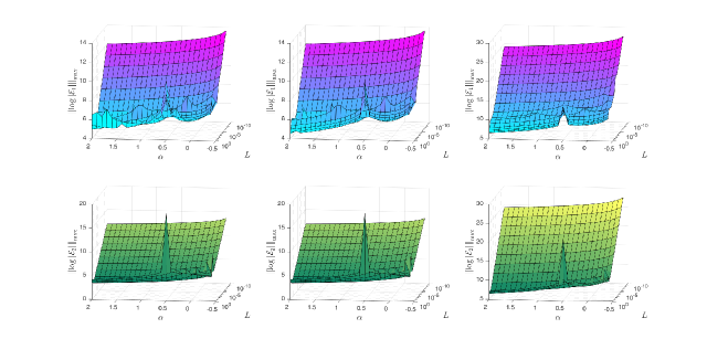
Figure 7: First row: The maximum logarithmic errors in evaluating the integrals $I_{1}$ (left), $I_{2}$ (middle), and $I_{3}$ (right) using the RG quadrature with $n=20$ against $\alpha$ and $L$ for $\alpha=-0.4$:$0.1$:$2$ and $L=10^{-10:1:-1},0.2$:$0.2$:$1$. Second row: The corresponding errors using the EG quadrature.

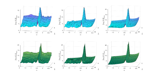
Figure 8: First row: The maximum logarithmic errors in evaluating the integrals $I_{1}$ (left), $I_{2}$ (middle), and $I_{3}$ (right) using the RG quadrature with $n=20$ against $\alpha$ and $L$ for $\alpha=-0.4$:$0.1$:$2$ and $L=2$:$2$:$10,15$:$5$:$50$. Second row: The corresponding errors using the EG quadrature.

All integrand functions are chosen to be sufficiently smooth and bounded on $\mathbb{R}_{0}^{+}$ to test whether the TG quadrature can provide exponential convergence rates, as expected with common GG quadratures based on standard Gegenbauer polynomials. Figures 1–6 show the maximum logarithmic error (MLE) associated with the approximation of each integral for several ranges of the parameters $\alpha,L$, and $n$, where $\mathcal{E}_{1:2}$ refers to the errors associated with the RG and EG quadratures, respectively. The accuracy of the TG quadrature increases as $n$ increases in all cases, and the numerical errors generally decay algebraically as $n$ increases but exhibit exponential convergence rates for $\alpha=0.5$ within a certain “optimal” range of $L$ values. Notice from the figures that the TG quadrature errors decrease exponentially as $L\to 0$ in all cases. In addition, as $L$ moves away from $0$, the RG quadrature errors generally rise and fall several times with two discerned patterns of global minimum values: (i) When the RG quadrature converges algebraically, the error global minimum value (EGMV) occurs when $L\in(10^{-2},1)\cup(3,6]$ and (ii) when the RG quadrature converges exponentially, the EGMV falls within the range $15<L<25$ with an approximate global minimum at $L=20$ based on the experimental data. The profile of the EG quadrature errors is slightly different from that of the RG quadrature as $L$ moves away from $0$ in the sense that: (i) When the EG quadrature converges algebraically, the EGMV occurs only when $L\in(10^{-2},1)$, and (ii) when the EG quadrature converges exponentially, the EGMV falls within the range $10<L<20$ with an approximate global minimum at $L=15$ based on the experimental data. Figures 7 and 8 give more insight into the error behavior relative to the parameter $\alpha$, where we can observe two important remarks: (i) When $L\to 0$, the quadrature errors are generally strictly decreasing as $\alpha$ decreases, so that the error approaches its minimum value as $\alpha\to-0.5$; (ii) when $L$ moves away from zero, the MLE profile exhibits a spike-like surface with a sharp spike located exactly at $\alpha=0.5$ indicating superior accuracy at this value among all other possible choices.

Assuming that both the optimal state and control variables are sufficiently smooth and bounded, the following rule of thumb sheds light on the optimal ordered pair of parameters $(\alpha,L)$ used by the TG-IS method for solving Problem $\mathscr{A}$.

Rule of Thumb 1.

The best possible approximations to the solutions of Problem $\mathscr{A}$ obtained by using the TG-IS method are most likely achieved when the TG collocation phase is performed at the TGG points set $\mathbb{TG}_{i,n}^{\alpha,L}$ for

$$(\alpha,L)\in\left\{\begin{array}[]{l}\left\{{1/2}\right\}\times(15,25),\quad\text{if }i=1,\\ \left\{{1/2}\right\}\times(10,20),\quad\text{if }i=2,\end{array}\right.$$ (7.3)

if the TG collocation is performed using a stretching mapping scaling parameter ($L>1$) since the TG quadrature generally converges exponentially in that range and the TG collocation is asymptotically stable for $n\in\,\mathrel{\mathop{\mathbb{Z}^{+}}\limits^{\vbox to0.0pt{\kern-2.0pt\hbox{$\scriptstyle\rightarrow$}\vss}}}$. In other words, the TG-IS method should be carried out using TL-based collocation at the TL-Gauss (TLG) points set $\mathbb{TG}_{i,n}^{1/2,L}$ for $L$ values as endorsed by Formula (7.3). On the other hand, the range of the parameters

$$(\alpha,L)\in\left\{\begin{array}[]{l}\mathrel{\mathop{\mathbb{R}}\limits^{\vbox to0.0pt{\kern-2.0pt\hbox{$\scriptstyle\rightarrow$}\vss}}}_{-1/2}\times(0,1),\quad\text{if }n\text{ is relatively small},\\ \{0\}\times(0,1),\quad\text{if }n\text{ is relatively large},\end{array}\right.$$ (7.4)

should be used $\forall i\in\mathbb{N}_{2}$, if the TG collocation is performed using a contracting mapping scaling parameter ($L<1$), since the TG quadrature truncation error is generally small for $L\in(0,1)$ with faster decay rates for decreasing $\alpha$ values, and the TG interpolation associated with $\alpha\in\,\mathrel{\mathop{\mathbb{R}}\limits^{\vbox to0.0pt{\kern-2.0pt\hbox{$\scriptstyle\rightarrow$}\vss}}}_{-1/2}$ is only stable for relatively small mesh grids but remains asymptotically stable for $\alpha\in\mathbb{R}_{0}^{+}$. In other words, the TG-IS method should be carried out using $(\alpha,L)\in\,\mathrel{\mathop{\mathbb{R}}\limits^{\vbox to0.0pt{\kern-2.0pt\hbox{$\scriptstyle\rightarrow$}\vss}}}_{-1/2}\times(0,1)$ for relatively small $n$ values, but should be performed using TC-based collocation at the TC-Gauss (TCG) points set $\mathbb{TG}_{i,n}^{0,L}$ for $L\in(0,1)$ and relatively large $n$ values, as prescribed by Formula (7.4).

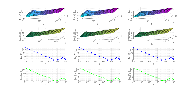
Figure 1: First row: The maximum logarithmic errors in evaluating the integrals $I_{1}$ (left), $I_{2}$ (middle), and $I_{3}$ (right) using the RG quadrature with $\alpha=-0.2$ against $N$ and $L$ for $N=2$:$20$ and $L=10^{-10:1:-1},0.2$:$0.2$:$1$. Second row: The corresponding errors using the EG quadrature. Third and fourth rows: The corresponding cross-sections of the maximum logarithmic errors that are shown in the first two rows with the plane $n=20$.

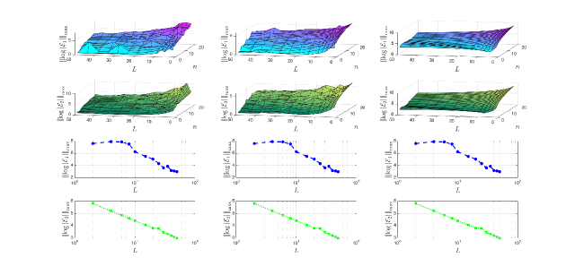
Figure 2: First row: The maximum logarithmic errors in evaluating the integrals $I_{1}$ (left), $I_{2}$ (middle), and $I_{3}$ (right) using the RG quadrature with $\alpha=-0.2$ against $N$ and $L$ for $N=2$:$20$ and $L=2$:$2$:$10,15$:$5$:$50$. Second row: The corresponding errors using the EG quadrature. Third and fourth rows: The corresponding cross-sections of the maximum logarithmic errors that are shown in the first two rows with the plane $n=20$.

Figure 3: First row: The maximum logarithmic errors in evaluating the integrals $I_{1}$ (left), $I_{2}$ (middle), and $I_{3}$ (right) using the RG quadrature with $\alpha=0$ against $N$ and $L$ for $N=2$:$20$ and $L=10^{-10:1:-1},0.2$:$0.2$:$1$. Second row: The corresponding errors using the EG quadrature. Third and fourth rows: The corresponding cross-sections of the maximum logarithmic errors that are shown in the first two rows with the plane $n=20$.

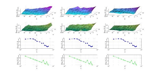
Figure 4: First row: The maximum logarithmic errors in evaluating the integrals $I_{1}$ (left), $I_{2}$ (middle), and $I_{3}$ (right) using the RG quadrature with $\alpha=0$ against $N$ and $L$ for $N=2$:$20$ and $L=2$:$2$:$10,15$:$5$:$50$. Second row: The corresponding errors using the EG quadrature. Third and fourth rows: The corresponding cross-sections of the maximum logarithmic errors that are shown in the first two rows with the plane $n=20$.

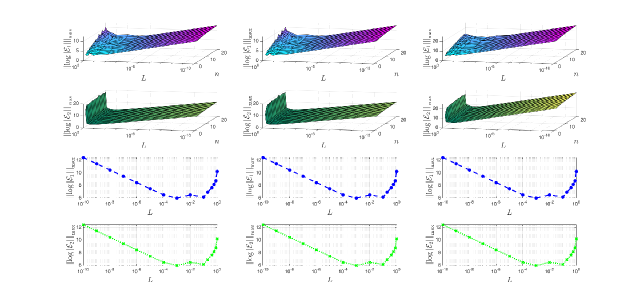
Figure 5: First row: The maximum logarithmic errors in evaluating the integrals $I_{1}$ (left), $I_{2}$ (middle), and $I_{3}$ (right) using the RG quadrature with $\alpha=0.5$ against $N$ and $L$ for $N=2$:$20$ and $L=10^{-10:1:-1},0.2$:$0.2$:$1$. Second row: The corresponding errors using the EG quadrature. Third and fourth rows: The corresponding cross-sections of the maximum logarithmic errors that are shown in the first two rows with the plane $n=20$.

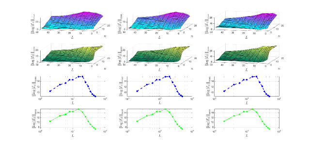
Figure 6: First row: The maximum logarithmic errors in evaluating the integrals $I_{1}$ (left), $I_{2}$ (middle), and $I_{3}$ (right) using the RG quadrature with $\alpha=0.5$ against $N$ and $L$ for $N=2$:$20$ and $L=2$:$2$:$10,15$:$5$:$50$. Second row: The corresponding errors using the EG quadrature. Third and fourth rows: The corresponding cross-sections of the maximum logarithmic errors that are shown in the first two rows with the plane $n=20$.

7.2 Benchmark Test Problems

In this section, we show the results of the EG-IS method for solving two benchmark test problems that were studied in [2]. Similar results of the EG-IS method can be obtained by the RG-IS method by following Rule of Thumb 1.

Problem 1. Consider Problem $\mathscr{A}$ with $\mathbf{Q}=\mathbf{I}_{5},\mathbf{R}=\mathbf{I}_{4},\mathbf{C}=[1,0,0,0,0],\,\mathbf{D}^{\top}=[0,1,1,1,1]$,

$$\mathbf{A}=\left[{\begin{array}[]{*{20}{c}}{-964.8}&{-33985.7}&{-33985.7}&{-33985.7}&{-33985.7}\\ 0&{-400}&0&0&0\\ 0&0&{-400}&0&0\\ 0&0&0&{-400}&0\\ 0&0&0&0&{-400}\end{array}}\right],\quad\text{and }\mathbf{B}=\left[{\begin{array}[]{*{20}{c}}0&0&0&0\\ {400}&0&0&0\\ 0&{400}&0&0\\ 0&0&{400}&0\\ 0&0&0&{400}\end{array}}\right].$$

This problem models a DCS linearized at a nominal point. Here $\bm{x}(t)=[p(t),A^{\top}_{1:4}\hbox to0.0pt{\raisebox{1.875pt}{\textcolor{black}{\rule{2.22223pt}{0.5pt}}}\hss}[t\hbox to0.0pt{\raisebox{1.875pt}{\textcolor{black}{\hskip 0.85358pt\rule{1.94443pt}{0.75pt}}}\hss}]]^{\top},\bm{u}(t)=u_{1:4}\hbox to0.0pt{\raisebox{1.875pt}{\textcolor{black}{\rule{2.22223pt}{0.5pt}}}\hss}[t\hbox to0.0pt{\raisebox{1.875pt}{\textcolor{black}{\hskip 0.85358pt\rule{1.94443pt}{0.75pt}}}\hss}]$, and $\bm{y}(t)=p(t)$, where $p(t)$ represents the change of the pressure within the combustion chamber of the gas generator, $A_{i}(t)$ denotes the $i$th nozzle’s area change from the nominal value, and $u_{i}(t)$ is the command to $i$th servo $\,\forall_{\mkern-6.0mue}\,i\in\mathbb{N}_{4}$; cf. [2]. Figure 9 shows a schematic diagram of the DCS. Note that the design-state constraint (3.1c) for this problem indicates that the sum of the changes in the throat area of the four nozzles must be zero while regulating the DCS. Cha et al. [2] solved the problem by solving the existence conditions for constraining output feedback gains and obtained the approximate optimal gain ${\mathbf{K}^{*}}^{\top}=[2.5125,-1.4994,-2.4537,1.4406]$ after a few trials. The corresponding optimal performance index was estimated to be $232.2286$, rounded to four decimal digits using the initial condition $\bm{x}(0)=[200,10,-10,5,-5]^{\top}$. Following the Rule of Thumb 1, we initially ran the TG-IS method with negative $\alpha$ values at low mesh grids for values of $0<L<1$ and then allowed $\alpha$ to gradually increase as the mesh size grows larger until it reaches zero value to maintain high accuracy and stability. Figure 10 shows plots of the approximate optimal state and control variables obtained by the proposed EG-IS method using $L=0.025$ and $(n,\alpha)\in\{(20,-0.45),(40,-0.1),(80,0)\}$ under the same initial condition. The figure clearly shows the exponential decay of all state variables in a short time, while the optimal control inputs initially increase rapidly for a short time period before decaying exponentially as the time increases. Figure 11 shows the plots of the corresponding size of the four nozzle throat area change sum, which nearly reaches the round-off error plateau, reflecting the satisfaction of the design state constraint (3.1c) with excellent accuracy. Figure 12 shows the corresponding plots of the MAEs when approximating the discrete weak dynamical system equations of NLP (5.3) at the collocation points. The corresponding approximate optimal output feedback gains obtained by the EG-IS method are listed in Table 1, where the recorded data converge to ${\bm{K}^{*}}^{\top}\approx[{0.01},-0.01,{0.005},{-0.005}]$, rounded to three decimal digits when $(n,\alpha)$ reaches $(80,0)$. The corresponding recorded elapsed times were about $13.65$ s, $3.04$ min, and $12.92$ min, respectively. Figure 13 shows the profile of the approximate optimal performance index for increasing $n$ values and gradually increasing nonpositive $\alpha$ values, where we observe that $J_{120}\approx 69.3811$, rounded to four decimal digits– a reduction of nearly $70$% of the estimated optimal cost function value obtained earlier in [2].

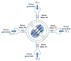
Figure 9: Schematic figure of the DCS as quoted from [2].

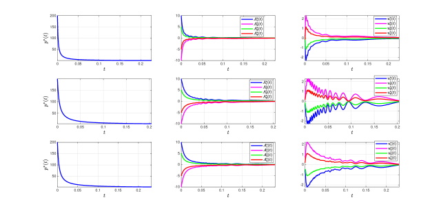
Figure 10: Plots of the approximate optimal state and control variables obtained by the EG-IS method using $L=0.025$ and $(n,\alpha)=(20,-0.45)$ (first row), $(n,\alpha)=(40,-0.1)$ (second row), and $(n,\alpha)=(80,0)$ (third row). The plots were generated using $100$ equally-spaced nodes from $0$ to ${}_{2}t_{n,n}^{\alpha}$.

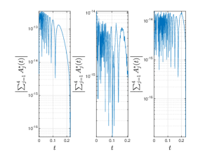
Figure 11: Plots of the size of the four nozzle’s throat area changes sum obtained by the EG-IS method using $L=0.025$ and $(n,\alpha)=(20,-0.45)$ (left), $(n,\alpha)=(40,-0.1)$ (middle), and $(n,\alpha)=(80,0)$ (right). The plots were generated using $100$ equally-spaced nodes from $0$ to ${}_{2}t_{n,n}^{\alpha}$.

Figure 12: Plots of the MAEs produced by the EG-IS method in approximating the discrete weak dynamical system equations of NLP (5.3) at the collocation points using $L=0.025$ and $(n,\alpha)=(20,-0.45)$ (left), $(n,\alpha)=(40,-0.1)$ (middle), and $(n,\alpha)=(80,0)$ (right). The plots were generated using $100$ equally-spaced nodes from $0$ to ${}_{2}t_{n,n}^{\alpha}$.

Table 1: The approximate optimal output feedback gains obtained by the EG-IS method using $L=0.025$ and several parameter values. All approximations are rounded to three decimal digits.

$(n,\alpha)=(20,-0.45)$	$(n,\alpha)=(40,-0.1)$	$(n,\alpha)=(80,0)$
$\bm{K}^{*}$	$\bm{K}^{*}$	$\bm{K}^{*}$
$\left[{\begin{array}[]{*{20}{c}}{0.008}\\ {-0.008}\\ {0.004}\\ {-0.004}\end{array}}\right]$	$\left[{\begin{array}[]{*{20}{c}}{0.009}\\ {-0.009}\\ {0.005}\\ {-0.005}\end{array}}\right]$	$\left[{\begin{array}[]{*{20}{c}}{0.010}\\ {-0.010}\\ {0.005}\\ {-0.005}\end{array}}\right]$

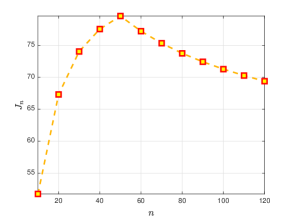
Figure 13: The approximate optimal performance index values against $n$ for $L=0.025$ and $(n,\alpha)\in\{(10,-0.4),(20,-0.3),(30,-0.2),(40,-0.1),(50:120,0)\}$.

Problem 2. Consider Problem $\mathscr{A}$ with $\mathbf{Q}=\text{diag}\left(50,100,100,50,0,0,1\right),\mathbf{R}=0.1\mathbf{I}_{2},\mathbf{D}^{\top}=[0,0,0,0,12,-1,0]$,

$$\mathbf{A}=\left[{\begin{array}[]{*{20}{c}}{-0.3220}&{0.0640}&{0.0364}&{-0.9917}&{0.0003}&{0.0008}&0\\ 0&0&1&{0.0037}&0&0&0\\ {-30.6492}&0&{-3.6784}&{0.6646}&{-0.7333}&{0.1315}&0\\ {8.5396}&0&{-0.0254}&{-0.4764}&{-0.0319}&{{\mathrm{}}-0.0620}&0\\ 0&0&0&0&{-20.2}&0&0\\ 0&0&0&0&0&{-20.2}&0\\ 0&0&0&{57.2958}&0&0&{-1}\end{array}}\right],\quad\mathbf{B}=\left[{\begin{array}[]{*{20}{c}}0&0\\ 0&0\\ 0&0\\ 0&0\\ {20.2}&0\\ 0&{20.2}\\ 0&0\end{array}}\right],$$

$$\text{and }\mathbf{C}=\left[{\begin{array}[]{*{20}{c}}0&0&0&{57.2958}&0&0&{-1}\\ 0&0&{57.2958}&0&0&0&0\\ {57.2958}&0&0&0&0&0&0\\ 0&{57.2958}&0&0&0&0&0\end{array}}\right].$$

This problem models the lateral dynamics of an F-16 aircraft linearized about the nominal flight condition (502 ft$/$s and 300 psf of dynamic pressure) retaining the lateral states sideslip $\beta$, bank angle $\phi$, roll rate $p$, and yaw rate $r$. Here $\bm{x}=[\beta,\phi,p,r,\delta_{a},\delta_{r},x_{w}]^{\top},\bm{u}=[u_{a},u_{r}]^{\top}$, and $\bm{y}=[r_{w},p,\beta,\phi]^{\top}$, where $\delta_{a}$ and $\delta_{r}$ are additional states introduced by the aileron and rudder actuators such that $(\delta_{a},\delta_{r})=\mu(u_{a},u_{r})$ with $\mu(t)=20.2/(t+20.2)$ and $r_{w}=t/(t+1)r$ is the washed-out yaw rate; cf. [2]. The design state constraint (3.1c) for this problem indicates that the aileron and the rudder are linked to each other by the functional relationship

$$\delta_{r}=12\delta_{a},$$ (7.5)

while regulating the system, which is known as an aileron-rudder interconnect (ARI) often used for stabilizing the system at a high angle of attack. Through the same approach, Cha et al. [2] obtained the approximate optimal gain

$${\mathbf{K}^{*}}=\left[{\begin{array}[]{*{20}{c}}{-0.2944}&{-0.0592}&{0.0357}&{-0.0271}\\ {-3.5333}&{-0.7109}&{0.4284}&{-0.3247}\end{array}}\right],$$

after a few trials. The corresponding optimal performance index was estimated to be $428.7008$, rounded to four decimal digits, using the initial condition $\bm{x}(0)=[0.5,\bm{\mathit{0}}_{6}^{\top}]^{\top}$. Following Rule of Thumb 1, we ran the EG-IS method using the recommended parameter values $(\alpha,L)=(1/2,15)$ for increasing mesh grids to achieve possibly the highest accuracy and stability based on the numerical observations prescribed in Section 7.1 and supported by the stability analysis. Figures 14 and 15 show the plots of the approximate optimal state and control variables obtained by the proposed EG-IS method using $(\alpha,L)=(1/2,15),n\in\{20,40,80\}$, and the same initial condition. Figure 16 shows the plots of the size of the errors by which the approximate optimal solutions fail to satisfy the ARI Condition (7.5). Figure 17 shows the corresponding plots of the MAEs in approximating the discrete weak dynamical system equations of NLP (5.3) at the collocation points. The corresponding approximate optimal output feedback gains obtained by the EG-IS method are shown in Table 2, where the recorded data converge to

$${\bm{K}^{*}}=\left[{\begin{array}[]{*{20}{c}}{0.026}&{0.054}&{0.136}&{-0.001}\\ {0.312}&{0.653}&{1.637}&{-0.015}\end{array}}\right],$$

rounded to three decimal digits, when $n$ reaches $80$. The corresponding recorded elapsed times were about $8.72$ s, $1.59$ min, and $21.32$ min, respectively. Figure 18 shows the profile of the approximate optimal performance index for increasing $n$ values, where we notice the exponential convergence of $J_{n}$, converging to nearly $316.8154$, rounded to four decimal digits, as early as $n$ reaches $20$– a reduction of nearly $26$% of the estimated optimal cost function value obtained earlier in [2].

Remark 7.1.

It is noteworthy to mention that for systems of small or moderate mesh size, the solutions by the RG-IS and EG-IS methods are easy and fast to implement; however, for large grids, their reduced NLPs become large-scale and MATLAB fmincon solver runs relatively slow. Fortunately, the EG-IS method converges to near-optimal results for sufficiently smooth solutions using a relatively small number of grids as shown by Tables 1 and 2, which allow us to achieve satisfactorily accurate approximations in relatively short running times. We expect a similar behavior for the RG-IS method by following Rule of Thumb 1.

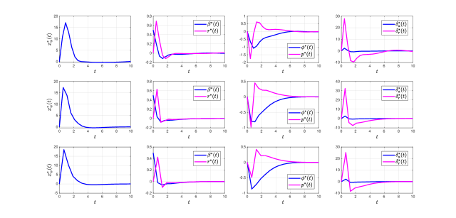
Figure 14: Plots of the approximate optimal state variables obtained by the EG-IS method using $(\alpha,L)=(1/2,15)$ and $n=20$ (first row), $n=40$ (second row), and $n=80$ (third row). The plots were generated using $100$ equally-spaced nodes from $0$ to ${}_{2}t_{n,n}^{0.5}$.

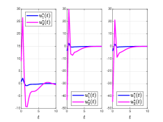
Figure 15: Plots of the approximate optimal control variables obtained by the EG-IS method using $(\alpha,L)=(1/2,15)$ and $n=20$ (left), $n=40$ (middle), and $n=80$ (right). The plots were generated using $100$ equally-spaced nodes from $0$ to ${}_{2}t_{n,n}^{0.5}$.

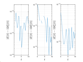
Figure 16: Plots of the size of the errors by which the approximate optimal solutions fail to satisfy the ARI Condition (7.5). The errors were produced by the EG-IS method using $(\alpha,L)=(1/2,15)$ and $n=20$ (left), $n=40$ (middle), and $n=80$ (right). The plots were generated using $100$ equally-spaced nodes from $0$ to ${}_{2}t_{n,n}^{0.5}$.

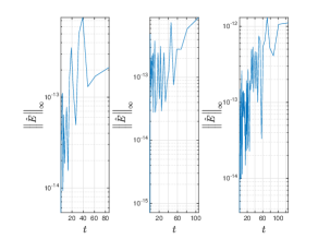
Figure 17: Plots of the MAEs produced by the EG-IS method in approximating the discrete weak dynamical system equations of NLP (5.3) at the collocation points using $(\alpha,L)=(1/2,15)$ and $n=20$ (left), $n=40$ (middle), and $n=80$ (right). The plots were generated using $100$ equally-spaced nodes from $0$ to ${}_{2}t_{n,n}^{0.5}$.

Table 2: The approximate optimal output feedback gains obtained by the EG-IS method using $(\alpha,L)=(1/2,15)$ and several $n$ values. All approximations are rounded to three decimal digits.

$n=20$	$n=40$	$n=80$
${\bm{K}^{*}}^{\top}$	${\bm{K}^{*}}^{\top}$	${\bm{K}^{*}}^{\top}$
$\left[{\begin{array}[]{*{20}{c}}{0.037}&{0.441}\\ {0.031}&{0.372}\\ {-0.017}&{-0.201}\\ {-0.001}&{-0.017}\end{array}}\right]$	$\left[{\begin{array}[]{*{20}{c}}{0.026}&{0.312}\\ {0.055}&{0.654}\\ {0.137}&{1.640}\\ {-0.001}&{-0.015}\end{array}}\right]$	$\left[{\begin{array}[]{*{20}{c}}{0.026}&{0.312}\\ {0.054}&{0.653}\\ {0.136}&{1.637}\\ {-0.001}&{-0.015}\end{array}}\right]$

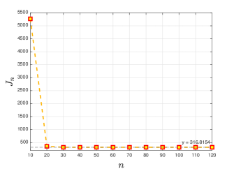
Figure 18: The approximate optimal performance index values against $n$ for $(\alpha,L)=(1/2,15)$ and $n=10$:$10$:$120$.

8 Conclusion

This study introduces two novel numerical methods for solving a class of infinite-horizon regulation problems governed by linear systems with state equality constraints and output feedback control. The proposed TG-IS method proved to be successful in practice and was capable of providing accurate numerical solutions with rapid convergence. In particular, the TG-IS method is more efficient than the TG-IPS method, which leads to NLPs with dimensions proportional to the square of the collocation mesh size, whereas the former method produces NLPs with dimensions that grow only linearly with the collocation mesh size. Another merit of the TG-IS method occurs in its ability to provide a useful means to avoid the derivation and solution of the sophisticated optimal gain design equations of Cha et al. [2] for the constrainable output feedback gains, which require either finding the optimal form of a nonunique basis matrix or fixing a basis matrix a priori before finding the optimal gain and then compare the effect of the various basis matrices on the performance of the controller via numerical simulations. Instead, the TG-IS method directly discretizes the integral form of the IHOC in its original domain via efficient collocation and highly accurate quadratures based on TG functions. Based on the rigorous stability analysis presented in B, we proved that the TG interpolation of a function is asymptotically stable for $\alpha\in\mathbb{R}_{0}^{+}$ under mild conditions. However, such schemes are asymptotically unstable for $(n,\alpha)\in\,\mathrel{\mathop{\mathbb{Z}^{+}}\limits^{\vbox to0.0pt{\kern-2.0pt\hbox{$\scriptstyle\rightarrow$}\vss}}}\times\mathrel{\mathop{\mathbb{R}}\limits^{\vbox to0.0pt{\kern-2.0pt\hbox{$\scriptstyle\rightarrow$}\vss}}}_{-1/2}$, especially when $\alpha\to-1/2$. These theoretical results, in addition to the extensive numerical simulations in Section 7.1, led to the foundation of Rule of Thumb 1, which gave us a practical way to optimize the performance of the TG-IS method by identifying the optimal ranges of the mesh size, the Gegenbauer index, and the mapping scaling parameter associated with the TG functions.

9 Future Work

One possible future research direction is to extend the application of the proposed methods to handle more general nonlinear IHOCs.

Appendix A Rational and Exponential Gegenbauer Functions

We define the RG and EG functions with ordered index pair $(\alpha,L)\in\,\mathrel{\mathop{\mathbb{R}}\limits^{\vbox to0.0pt{\kern-2.0pt\hbox{$\scriptstyle\rightarrow$}\vss}}}_{-1/2}\times\mathbb{R}^{+}$ by

$$\mathcal{G}_{i,n}^{\alpha,L}(t)=G_{n}^{\alpha}\left(T_{i,L}(t)\right)\quad\forall(i,n,t)\in\mathbb{N}_{2}\times\mathbb{Z}_{0}^{+}\times\mathbb{R}_{0}^{+},$$ (A.1)

respectively, where

$${T_{i,L}}(t)=\left\{\begin{array}[]{l}(t-L)/(t+L),\quad i=1,\\ 1-2{e^{-t/L}},\quad i=2,\end{array}\right.$$ (A.2)

and $L$ is a mapping scaling parameter. Both functions are referred to collectively by “the TG functions,” or more specifically by “the TG functions with ordered index pair $(\alpha,L)$.” The transformed Chebyshev (TC) function and transformed Legendre (TL) function are special cases of the TG function for the Gegenbauer parameter values $\alpha=0$ and $\alpha=1/2$, respectively. The TG function $\mathcal{G}_{i,n}^{\alpha,L}$ appears as an eigensolution to the following singular Sturm-Liouville (SSL) problem on $\mathbb{R}_{0}^{+}$:

$$\frac{1}{{T^{\prime}_{i,L}(t)}}\frac{d}{{dt}}\left[{\frac{{{{\left({1-T_{i,L}^{2}(t)}\right)}^{\alpha+1/2}}}}{{{T^{\prime}_{i,L}}(t)}}{\mathcal{G}^{\prime}_{i,n}}^{\alpha,L}(t)}\right]+n\left({n+2\alpha}\right){\left({1-T_{i,L}^{2}(t)}\right)^{\alpha-1/2}}\mathcal{G}_{i,n}^{\alpha,L}(t)=0\quad\forall i\in\mathbb{N}_{2},$$ (A.3)

where

$${T^{\prime}_{i,L}}(t)=\left\{\begin{array}[]{l}2L/(t+L)^{2},\quad i=1,\\ 2{e^{-t/L}}/L,\quad i=2.\end{array}\right.$$ (A.4)

In particular, the RG and EG functions are eigenfunctions of the following SSL problems

$$\frac{1}{L}{(t+L)^{2}}\frac{d}{{dt}}\left[{t\,{{\left({\frac{t}{{{{\left({t+L}\right)}^{2}}}}}\right)}^{\alpha-\frac{1}{2}}}{\mathcal{G}^{\prime}_{1,n}}^{\alpha,L}(t)}\right]+n\left({n+2\alpha}\right){\left({\frac{t}{{{{\left({t+L}\right)}^{2}}}}}\right)^{\alpha-\frac{1}{2}}}\mathcal{G}_{1,n}^{\alpha,L}(t)=0,$$ (A.5a)

$$\frac{{{L^{2}}}}{4}{e^{t/L}}\frac{d}{{dt}}\left[{{e^{\frac{t}{L}}}\,{{\left({1-{{\left({1-2{e^{-\frac{t}{L}}}}\right)}^{2}}}\right)}^{\alpha+\frac{1}{2}}}{\mathcal{G}^{\prime}_{2,n}}^{\alpha,L}(t)}\right]+n\left({n+2\alpha}\right){\left({1-{{\left({1-2{e^{-\frac{t}{L}}}}\right)}^{2}}}\right)^{\alpha-\frac{1}{2}}}\mathcal{G}_{2,n}^{\alpha,L}(t)=0,$$ (A.5b)

which can be restated as follows:

$$\left({t+L}\right)\left[{2t\left({t+L}\right){\mathcal{G}^{\prime\prime}_{1,n}}^{\alpha,L}(t)+\left({(2\alpha+1)L+(3-2\alpha)t}\right){\mathcal{G}^{\prime}_{1,n}}^{\alpha,L}(t)}\right]+2Ln\left({n+2\alpha}\right)\mathcal{G}_{1,n}^{\alpha,L}(t)=0,$$ (A.6a)

$$L\left[{2L\left({{{e}^{t/L}}-1}\right){\mathcal{G}^{\prime\prime}_{2,n}}^{\alpha,L}(t)+\left({4\alpha+\left({1-2\alpha}\right){e^{t/L}}}\right){\mathcal{G}^{\prime}_{2,n}}^{\alpha,L}(t)}\right]+2n\left({n+2\alpha}\right)\mathcal{G}_{2,n}^{\alpha,L}(t)=0,$$ (A.6b)

respectively. The weight functions of the TG functions are given in respective order by

$$w^{\alpha,L}_{1}(t)=\frac{4^{\alpha}L^{\alpha+1/2}t^{\alpha-1/2}}{(t+L)^{2\alpha+1}},\quad w^{\alpha,L}_{2}(t)=\frac{2}{L}{e^{-t/L}}{\left[{1-{{\left({1-2{e^{-t/L}}}\right)}^{2}}}\right]^{\alpha-1/2}}.$$ (A.7)

The TG functions are orthogonal with respect to the weight functions $w^{\alpha,L}_{1}$ and $w^{\alpha,L}_{2}$, respectively, and their orthogonality relations are defined by

$$\mathcal{I}_{\mathbb{R}_{0}^{+}}^{(t)}{\left(\mathcal{G}_{i,m}^{\alpha,L}\,\mathcal{G}_{i,n}^{\alpha,L}w^{\alpha,L}_{i}\right)}=\lambda^{\alpha}_{n}\delta_{mn}\quad\forall i\in\mathbb{N}_{2},\quad\{m,n\}\subset\mathbb{Z}_{0}^{+},$$ (A.8)

where

$$\lambda^{\alpha}_{n}=\frac{2^{2\alpha-1}n!\Gamma^{2}{(\alpha+\frac{1}{2})}}{(n+\alpha)\Gamma(n+2\alpha)}.$$ (A.9)

Therefore, the TG functions form an orthogonal basis set for $L_{w_{i}^{\alpha,L}}^{2}\left(\mathbb{R}_{0}^{+}\right)$ so that the TG expansion of a function $f\in L_{w_{i}^{\alpha,L}}^{2}\left(\mathbb{R}_{0}^{+}\right)$ can be written as

$$f(t)={{\hat{f}}_{0:\infty}}\,\mathcal{G}_{i,0:\infty}^{\alpha,L}\hbox to0.0pt{\raisebox{1.875pt}{\textcolor{black}{\rule{2.22223pt}{0.5pt}}}\hss}[t\hbox to0.0pt{\raisebox{1.875pt}{\textcolor{black}{\hskip 0.85358pt\rule{1.94443pt}{0.75pt}}}\hss}]:\quad{\hat{f}_{k}}=\frac{1}{{\lambda_{k}^{\alpha}}}\mathcal{I}_{\mathbb{R}_{0}^{+}}^{(t)}\left({f\,\mathcal{G}_{i,k}^{\alpha,L}w_{i}^{\alpha,L}}\right)\quad\forall(k,i)\in\mathbb{Z}_{0}^{+}\times\mathbb{N}_{2}.$$ (A.10)

The TG functions can be generated by the following three-term recurrence relation

$$\mathcal{G}_{i,0}^{\alpha,L}(t)=1,\quad\mathcal{G}_{i,1}^{\alpha,L}(t)=T_{i,L}(t),\quad(n+2\alpha)\,\mathcal{G}_{i,n+1}^{\alpha,L}(t)=2(n+\alpha)T_{i,L}(t)\,\mathcal{G}_{i,n}^{\alpha,L}(t)-n\,\mathcal{G}_{i,n-1}^{\alpha,L}(t)\quad\forall i\in\mathbb{N}_{2},\quad n\geq 1.$$ (A.11)

In particular, the first four RG and EG functions are given by

$$\mathcal{G}_{1,0}^{\alpha,L}(t)=1,\quad\mathcal{G}_{1,1}^{\alpha,L}(t)=\frac{t-L}{t+L},\quad\mathcal{G}_{1,2}^{\alpha,L}(t)=\frac{1}{{1+2\alpha}}\left[{2\left({1+\alpha}\right){{\left({\frac{{t-L}}{{t+L}}}\right)}^{2}}-1}\right],\quad\mathcal{G}_{1,3}^{\alpha,L}(t)=\frac{1}{{{{\left({t+L}\right)}^{3}}}}\left[{{{\left({t-L}\right)}^{3}}-\frac{{12Lt\left({t-L}\right)}}{{1+2\alpha}}}\right],$$ (A.12a)

$$\mathcal{G}_{2,0}^{\alpha,L}(t)=1,\quad\mathcal{G}_{2,1}^{\alpha,L}(t)=1-2e^{-t/L},\quad\mathcal{G}_{2,2}^{\alpha,L}(t)=\frac{1}{{1+2\alpha}}\left[{2\left({1+\alpha}\right){{\left({1-2{e^{-\frac{t}{L}}}}\right)}^{2}}-1}\right],$$ (A.12b)

$$\mathcal{G}_{2,3}^{\alpha,L}(t)=\frac{1}{{1+2\alpha}}\left[{{e^{-\frac{{3t}}{L}}}\left({{e^{\frac{t}{L}}}-2}\right)\left({8\left({2+\alpha}\right)\left({1-{e^{\frac{t}{L}}}}\right)+\left({1+2\alpha}\right){e^{\frac{{2t}}{L}}}}\right)}\right].$$ (A.12c)

We define $\mathscr{T}_{i,n}^{\alpha,L}=\operatorname{span}\left\{\mathcal{G}_{i,1}^{\alpha,L},\mathcal{G}_{i,2}^{\alpha,L},\ldots,\mathcal{G}_{i,n}^{\alpha,L}\right\}$. We also define $\mathbb{TG}_{i,n}^{\alpha,L}=\left\{{}_{i}^{L}t_{n,0:n}^{\alpha}:{}_{i}^{L}t_{n,j}^{\alpha}=T_{i,L}^{-1}(x_{n,j}^{\alpha})\right\}$ to be the zeros set of the TG function with ordered index pair $(\alpha,L)$ (or simply the TGG points set) $\,\forall_{\mkern-6.0mua}\,n\in\mathbb{Z}^{+},i\in\mathbb{N}_{2}$, where

$${T_{i,L}^{-1}}(x)=\left\{\begin{array}[]{l}L(1+x)/(1-x),\quad i=1,\\ L\ln[2/(1-x)],\quad i=2.\end{array}\right.$$ (A.13)

In particular, we refer to the TGG points sets $\mathbb{TG}_{i,n}^{\alpha,L}\,\forall i\in\mathbb{N}_{2}$ by the RG-Gauss (RGG) and EG-Gauss (EGG) points sets, respectively. The following lemma provides the TGG quadrature formula of a function $f\in\mathscr{T}_{i,2n+1}^{\alpha,L}$, which is useful for the derivation of the proposed TG-IPS and TG-IS methods.

Lemma A.1.

The TGG quadrature of a function $f\in\mathscr{T}_{i,2n+1}^{\alpha,L}$ is given by

$$\mathcal{I}_{\mathbb{R}_{0}^{+}}^{(t)}\left(f\,w^{\alpha,L}_{i}\right)={}_{i}\bm{\varpi}^{\alpha,L}_{n}f^{\alpha,L}_{i,n,0:n}\quad\forall(i,n,\alpha,L)\in\mathbb{N}_{2}\times\mathbb{Z}_{0}^{+}\times\mathrel{\mathop{\mathbb{R}}\limits^{\vbox to0.0pt{\kern-2.0pt\hbox{$\scriptstyle\rightarrow$}\vss}}}_{-1/2}\times\mathbb{R}^{+},$$ (A.14)

where ${}_{i}\bm{\varpi}^{\alpha,L}_{n}={}_{i}\varpi^{\alpha,L}_{n,0:n}$:

$${}_{i}\varpi^{\alpha,L}_{n,j}=1/\left[{\lambda^{\alpha}_{0:n}}^{\div}\left(\mathcal{G}_{i,0:n}^{\alpha,L}\hbox to0.0pt{\raisebox{1.875pt}{\textcolor{black}{\rule{2.22223pt}{0.5pt}}}\hss}[{}_{i}^{L}t^{\alpha}_{n,j}\hbox to0.0pt{\raisebox{1.875pt}{\textcolor{black}{\hskip 0.85358pt\rule{1.94443pt}{0.75pt}}}\hss}]\right)_{(2)}\right]\quad\forall(i,j)\in\mathbb{N}_{2}\times\mathbb{J}_{n}.$$ (A.15)

It is easy to show that ${}_{i}\bm{\varpi}^{\alpha,L}_{n}=\bm{\varpi}^{\alpha}_{n}\,\forall i\in\mathbb{N}_{2}$, where $\bm{\varpi}^{\alpha}_{n}=\varpi^{\alpha}_{n,0:n}$ is the usual GG quadrature weight vector with elements

$$\varpi^{\alpha}_{n,j}=1/\left[{\lambda^{\alpha}_{0:n}}^{\div}\left(G_{0:n}^{\alpha}\hbox to0.0pt{\raisebox{1.875pt}{\textcolor{black}{\rule{2.22223pt}{0.5pt}}}\hss}[x^{\alpha}_{n,j}\hbox to0.0pt{\raisebox{1.875pt}{\textcolor{black}{\hskip 0.85358pt\rule{1.94443pt}{0.75pt}}}\hss}]\right)_{(2)}\right]\quad\forall j\in\mathbb{J}_{n}.$$ (A.16)

The discrete inner product and the discrete norm associated with the TGG interpolation points are given by

$$(u,v)_{w_{i}^{\alpha,L},n}=\sum_{j\in\mathbb{J}_{n}}{u_{i,n,j}^{\alpha,L}v_{i,n,j}^{\alpha,L}\,\varpi_{n,j}^{\alpha}},\quad\left\|u\right\|_{w_{i}^{\alpha,L},n}=(u,u)_{w_{i}^{\alpha,L},n}^{1/2}\quad\forall\{u,v\}\subset\text{Def}\left(\mathbb{R}_{0}^{+}\right),$$ (A.17)

respectively.

Appendix B TG Interpolation/Collocation and Its Stability

Using the discrete inner products derived in A, we can derive the TG interpolant

$$I_{n}f(t)={{\tilde{f}}_{0:n}}\,\mathcal{G}_{i,0:n}^{\alpha,L}\hbox to0.0pt{\raisebox{1.875pt}{\textcolor{black}{\rule{2.22223pt}{0.5pt}}}\hss}[t\hbox to0.0pt{\raisebox{1.875pt}{\textcolor{black}{\hskip 0.85358pt\rule{1.94443pt}{0.75pt}}}\hss}],$$ (B.1)

that satisfies the interpolation condition

$$I_{n}f_{i,n,0:n}^{\alpha,L}=f_{i,n,0:n}^{\alpha,L}\quad\forall i\in\mathbb{N}_{2}.$$ (B.2)

The orthogonality of the TG basis functions allows us to find the coefficients of the TG interpolant in the following form:

$$\tilde{f}_{k}=\frac{(I_{n}f,\mathcal{G}_{i,k}^{\alpha,L})_{w_{i}^{\alpha,L},n}}{\left\|\mathcal{G}_{i,k}^{\alpha,L}\right\|_{w_{i}^{\alpha,L},n}^{2}}=\frac{(f,\mathcal{G}_{i,k}^{\alpha,L})_{w_{i}^{\alpha,L},n}}{\left\|\mathcal{G}_{i,k}^{\alpha,L}\right\|_{w_{i}^{\alpha,L},n}^{2}}\quad\forall(k,i)\in\mathbb{J}_{n}\times\mathbb{N}_{2}.$$ (B.3)

The following lemma is needed to investigate the stability of TG interpolation.

Lemma B.1.

The Christoffel numbers for the Gegenbauer weight function $w^{\alpha}$ are asymptotically bounded by

$$\varpi_{n,j}^{\alpha}\,\hbox{\lower 2.58334pt\hbox{$\leq$}\hbox to0.0pt{\hss\raise 2.58334pt\hbox{$\sim$}}}\,\varpi^{\text{upp},+}=\frac{\pi}{{n+1}}\quad\forall(n,j,\alpha)\in\,\mathrel{\mathop{\mathbb{Z}^{+}}\limits^{\vbox to0.0pt{\kern-2.0pt\hbox{$\scriptstyle\rightarrow$}\vss}}}\times\mathbb{J}_{n}\times\mathbb{R}_{0}^{+}.$$ (B.4)

Proof.

First notice that

$$\frac{d}{{d\alpha}}\lambda_{j}^{\alpha}=\frac{{{2^{2\alpha-1}}{\Gamma^{2}}\left({\alpha+\frac{1}{2}}\right)\Gamma\left({j+1}\right)}}{{{{\left({j+\alpha}\right)}^{2}}\Gamma\left({j+2\alpha}\right)}}\left[{\left({j+\alpha}\right)\left({\ln 4+2\left({\digamma\left({\alpha+\frac{1}{2}}\right)-\digamma\left({j+2\alpha}\right)}\right)}\right)-1}\right]<0\quad\forall(j,\alpha)\in\mathbb{Z}_{0}^{+}\times\mathrel{\mathop{\mathbb{R}}\limits^{\vbox to0.0pt{\kern-2.0pt\hbox{$\scriptstyle\rightarrow$}\vss}}}_{-1/2},$$ (B.5a)

$$\frac{d}{{dj}}\lambda_{j}^{\alpha}=\frac{{{2^{2\alpha-1}}\Gamma^{2}{\left({\alpha+\frac{1}{2}}\right)}\Gamma\left({j+1}\right)}}{{{{\left({j+\alpha}\right)}^{2}}\Gamma\left({j+2\alpha}\right)}}\left[{\left({j+\alpha}\right)\left({{H_{j}}-{H_{j+2\alpha-1}}}\right)-1}\right]<0\quad\forall(j,\alpha)\in\mathbb{Z}_{0}^{+}\times\mathbb{R}^{+},$$ (B.5b)

since $\digamma$ and $H_{x}$ are both strictly increasing with respect to their arguments. Therefore, $\lambda_{j}^{\alpha}$ is strictly decreasing with respect to its indices $\forall(j,\alpha)\in\mathbb{Z}_{0}^{+}\times\mathbb{R}^{+}$; cf. Figure 19 for a sketch of $\lambda_{j}^{\alpha}$ and its reciprocal. This result together with the fact that $\left\|G_{k}^{\alpha}\right\|_{\infty}\leq 1\,\forall\alpha\in\mathbb{R}_{0}^{+}$; cf. [18, Lemma 2.1], implies

$$\varpi_{n,j}^{\alpha}=1/\left[{\lambda^{\alpha}_{0:n}}^{\div}\left(G_{0:n}^{\alpha}\hbox to0.0pt{\raisebox{1.875pt}{\textcolor{black}{\rule{2.22223pt}{0.5pt}}}\hss}[x^{\alpha}_{n,j}\hbox to0.0pt{\raisebox{1.875pt}{\textcolor{black}{\hskip 0.85358pt\rule{1.94443pt}{0.75pt}}}\hss}]\right)_{(2)}\right]\,\hbox{\lower 2.58334pt\hbox{$<$}\hbox to0.0pt{\hss\raise 1.29167pt\hbox{$\sim$}}}\,\frac{1}{{(n+1){{\left({\lambda_{0}^{0}}\right)}^{-1}}}}=\varpi^{\text{upp},+}\quad\forall(n,j,\alpha)\in\,\mathrel{\mathop{\mathbb{Z}^{+}}\limits^{\vbox to0.0pt{\kern-2.0pt\hbox{$\scriptstyle\rightarrow$}\vss}}}\times\mathbb{J}_{n}\times\mathbb{R}^{+}.$$ (B.6)

On the other hand, recall that

$$\lambda_{j}^{0}=\left\{\begin{array}[]{l}\pi,\quad j=0,\\ \pi/2,\quad j\in\mathbb{Z}^{+},\end{array}\right.$$ (B.7)

and

$$\varpi_{n,j}^{0}=\varpi^{\text{upp},+}\quad\forall j\in\mathbb{Z}_{0}^{+}.$$ (B.8)

The proof is established by combining the results of (B.6) and (B.8). ∎

Figures 20 and 21 show the profiles of $\varpi_{100,j}^{\alpha}$ for $n\in\{100,101\},j\in\mathbb{J}_{n}$, and several positive $\alpha$ values. The figures show clearly the symmetrical property of $\varpi_{n,j}^{\alpha}$ about the $j=n/2$ axis for positive $\alpha$ values with maximum values at $j=\left\lfloor{n/2}\right\rfloor\,\forall n\in\mathbb{Z}^{+}$. Initially, the family of curves appears as parabolas that open downward for $\alpha\in(0,1/2]$ with the axis of symmetry $j=\left\lfloor{n/2}\right\rfloor\,\forall n\in\mathbb{Z}^{+}$, and then transform into bell-shaped curves for $\alpha>1/2$ that nearly die out near the boundaries $j=0,n$ such that $\varpi_{n,j}^{\alpha}$ becomes almost nonzero only on a small subdomain centered at $j=n/2$ for increasing values of $\alpha$.

Remark B.1.

Lemma B.1 agrees with the earlier bounds of the $n$-point GG quadrature weights obtained in [19], which shows that

$$\varpi_{n,j}^{\alpha}\leq\frac{\pi}{{n+\alpha}}\sin^{2\alpha}\theta_{n,j}^{\alpha}\quad\forall\alpha\in\mathbf{\Omega}_{1},$$ (B.9)

where $x_{n,j}^{\alpha}=-\cos\theta_{n,j}^{\alpha}$.

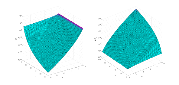
Figure 19: The surfaces of $\lambda_{n}^{\alpha}$ and its reciprocal on the discrete rectangular domain $\{(n,\alpha):n=1$:$100,\alpha=0.01$:$0.0999$:$10\}$.

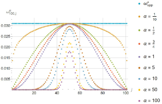
Figure 20: Plot of $\varpi_{100,j}^{\alpha}$ for $(j,\alpha)\in\mathbb{J}_{100}\times\{0.1,0.5,1,5,10,50,100\}$.

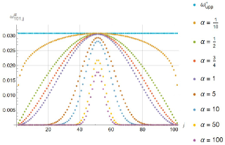
Figure 21: Plot of $\varpi_{101,j}^{\alpha}$ for $(j,\alpha)\in\mathbb{J}_{101}\times\{0.1,0.5,1,5,10,50,100\}$.

The following two theorems highlight the stability of TG interpolation for $\alpha\in\mathbb{R}_{0}^{+}$ using several space norms.

Theorem B.2.

$\,\forall_{\mkern-6.0mua}\,u\in L_{w_{i}^{\alpha,L}}^{2}\left(\mathbb{R}_{0}^{+}\right)$, we have

$${\left\|{I_{n}}u\right\|_{L_{w_{i}^{\alpha,L}}^{2}\left(\mathbb{R}_{0}^{+}\right)}}\,\hbox{\lower 2.58334pt\hbox{$\leq$}\hbox to0.0pt{\hss\raise 2.58334pt\hbox{$\sim$}}}\,\sqrt{\pi}\,{\left\|u\right\|_{L^{\infty}\left(\mathbb{R}_{0}^{+}\right)}}\quad\forall(n,\alpha,L,i)\in\,\mathrel{\mathop{\mathbb{Z}^{+}}\limits^{\vbox to0.0pt{\kern-2.0pt\hbox{$\scriptstyle\rightarrow$}\vss}}}\times\mathbb{R}_{0}^{+}\times\mathbb{R}^{+}\times\mathbb{N}_{2}.$$ (B.10)

Proof.

The proof is straightforward by using Lemma B.1 and realizing that

$${\left\|{I_{n}}u\right\|_{L_{w_{i}^{\alpha,L}}^{2}\left(\mathbb{R}_{0}^{+}\right)}^{2}}=\left\|I_{n}u\right\|_{w_{i}^{\alpha,L},n}^{2}=\sum_{j\in\mathbb{J}_{n}}{\left(u_{i,n,j}^{\alpha}\right)^{2}\varpi_{n,j}^{\alpha}}\,\hbox{\lower 2.58334pt\hbox{$\leq$}\hbox to0.0pt{\hss\raise 2.58334pt\hbox{$\sim$}}}\,\varpi^{\text{upp},+}\sum_{j\in\mathbb{J}_{n}}{\left(u_{i,n,j}^{\alpha}\right)^{2}}\quad\forall n\in\,\mathrel{\mathop{\mathbb{Z}^{+}}\limits^{\vbox to0.0pt{\kern-2.0pt\hbox{$\scriptstyle\rightarrow$}\vss}}},$$ (B.11)

whence the proof is established. ∎

Theorem B.3.

$\,\forall_{\mkern-6.0mua}\,u\in H^{1}_{w_{i}^{\alpha,L}}\left(\mathbb{R}_{0}^{+}\right)\,\exists\,c\in\mathbb{R}^{+}:$

$${\left\|{I_{n}}u\right\|_{L_{w_{i}^{\alpha,L}}^{2}\left(\mathbb{R}_{0}^{+}\right)}}<c\left({\left\|u\right\|_{L_{w_{i}^{\alpha,L}}^{2}\left(\mathbb{R}_{0}^{+}\right)}}+\frac{1}{n}\left\|\sqrt{(t+1)\sqrt{t}}\,u^{\prime}\right\|_{L^{2}\left(\mathbb{R}_{0}^{+}\right)}\right)\quad\forall(n,\alpha,L,i)\in\,\mathrel{\mathop{\mathbb{Z}^{+}}\limits^{\vbox to0.0pt{\kern-2.0pt\hbox{$\scriptstyle\rightarrow$}\vss}}}\times\mathbb{R}_{0}^{+}\times\mathbb{R}^{+}\times\mathbb{N}_{2}.$$ (B.12)

Proof.

Let $t=(1+\cos\theta)/(1-\cos\theta),\hat{u}(\theta)=u\left((1+\cos\theta)/(1-\cos\theta)\right)$, and $\mathscr{K}_{n,j}=[2\pi j/(2n+1),(2j+1)\pi/(2n+1)]\,\forall j\in\mathbb{J}_{n}$. Then the asymptotic inequality (B.11) yields

$${\left\|{I_{n}}u\right\|_{L_{w_{i}^{\alpha,L}}^{2}\left(\mathbb{R}_{0}^{+}\right)}^{2}}\,\hbox{\lower 2.58334pt\hbox{$\leq$}\hbox to0.0pt{\hss\raise 2.58334pt\hbox{$\sim$}}}\,\varpi^{\text{upp},+}\sum_{j\in\mathbb{J}_{n}}{\mathop{\sup}\limits_{\theta\in\mathscr{K}_{n,j}}\hat{u}^{2}(\theta)}\quad\forall(n,\alpha,L,i)\in\,\mathrel{\mathop{\mathbb{Z}^{+}}\limits^{\vbox to0.0pt{\kern-2.0pt\hbox{$\scriptstyle\rightarrow$}\vss}}}\times\mathbb{R}_{0}^{+}\times\mathbb{R}^{+}\times\mathbb{N}_{2}.$$ (B.13)

The rest of the proof follows the proof of [20, Theorem 4.1]. ∎

Theorems B.2 and B.3 show that the TG interpolation of a function is asymptotically stable for $\alpha\in\mathbb{R}_{0}^{+}$ under mild conditions. To investigate the stability of TG interpolation for $\alpha\in\,\mathbb{R}_{-1/2}^{-}$, we shall need the following lemma.

Lemma B.2.

The Christoffel numbers for the Gegenbauer weight function $w^{\alpha}$ are asymptotically bounded by

$$\varpi_{n,j}^{\alpha}<\varpi^{\text{upp,-}}_{n,\alpha}\quad\forall(n,j,\alpha)\in\,\mathrel{\mathop{\mathbb{Z}^{+}}\limits^{\vbox to0.0pt{\kern-2.0pt\hbox{$\scriptstyle\rightarrow$}\vss}}}\times\mathbb{J}_{n}\times\mathbb{R}_{-1/2}^{-},$$ (B.14)

where

$$\varpi^{\text{upp,-}}_{n,\alpha}=\frac{\Gamma^{2}(\alpha+1/2)}{2\,n^{1+2\alpha}}.$$ (B.15)

Proof.

The sharp lower bound for the gamma function [9, Inequality (96)] yields

$$\Gamma(n+2\alpha)>\sqrt{2\pi\,{\gamma_{n}}}{\left({\frac{{{\gamma_{n}}}}{e}}\right)^{{\gamma_{n}}}}{\left[{{\gamma_{n}}\sinh\left({\frac{1}{{{\gamma_{n}}}}}\right)}\right]^{{\gamma_{n}}/2}}\sim\sqrt{2\pi\,{\gamma_{n}}}{\left({\frac{{{\gamma_{n}}}}{e}}\right)^{{\gamma_{n}}}}\quad\forall n\in\,\mathrel{\mathop{\mathbb{Z}^{+}}\limits^{\vbox to0.0pt{\kern-2.0pt\hbox{$\scriptstyle\rightarrow$}\vss}}},$$ (B.16)

where $\gamma_{n}=n+2\alpha-1$. Using Stirling’s asymptotic approximation

$$n!\sim\sqrt{2\pi n}\,{\left({\frac{n}{e}}\right)^{n}}\quad\forall n\in\,\mathrel{\mathop{\mathbb{Z}^{+}}\limits^{\vbox to0.0pt{\kern-2.0pt\hbox{$\scriptstyle\rightarrow$}\vss}}},$$ (B.17)

we can easily show that

$$\frac{n!}{\Gamma(n+2\alpha)}\,\hbox{\lower 2.58334pt\hbox{$<$}\hbox to0.0pt{\hss\raise 1.29167pt\hbox{$\sim$}}}\,e^{2\alpha-1}\frac{n^{n+1/2}}{\gamma_{n}^{\gamma_{n}+1/2}}\quad\forall n\in\,\mathrel{\mathop{\mathbb{Z}^{+}}\limits^{\vbox to0.0pt{\kern-2.0pt\hbox{$\scriptstyle\rightarrow$}\vss}}}.$$ (B.18)

Therefore,

$$\lambda_{n}^{\alpha}\,\hbox{\lower 2.58334pt\hbox{$<$}\hbox to0.0pt{\hss\raise 1.29167pt\hbox{$\sim$}}}\,(2e)^{2\alpha-1}\Gamma^{2}(\alpha+1/2)\frac{n^{n+1/2}}{(n+\alpha)\,\gamma_{n}^{\gamma_{n}+1/2}} <(2e)^{2\alpha-1}\Gamma^{2}(\alpha+1/2)\frac{n^{n+1/2}}{n^{n+2\alpha+1/2}\left[1+(2\alpha-1)/n\right]^{n+2\alpha+1/2}}$$

$$\sim 2^{2\alpha-1}\Gamma^{2}(\alpha+1/2)\,n^{-2\alpha}\quad\forall n\in\,\mathrel{\mathop{\mathbb{Z}^{+}}\limits^{\vbox to0.0pt{\kern-2.0pt\hbox{$\scriptstyle\rightarrow$}\vss}}}.$$ (B.19)

Recall from Ineq. (B.5a) that $\lambda_{j}^{\alpha}$ is strictly decreasing with respect to $\alpha\,\forall(j,\alpha)\in\mathbb{Z}_{0}^{+}\times\mathrel{\mathop{\mathbb{R}}\limits^{\vbox to0.0pt{\kern-2.0pt\hbox{$\scriptstyle\rightarrow$}\vss}}}_{-1/2}$. Formula (B.5b), on the other hand, shows that $\displaystyle{\frac{d}{{dj}}}\lambda_{j}^{\alpha}>0\,\forall(j,\alpha)\in\mathbb{Z}_{0}^{+}\times\mathbb{R}_{-1/2}^{-}$, so that $\lambda_{j}^{\alpha}$ is strictly increasing with respect to $j\,\forall(j,\alpha)\in\mathbb{Z}_{0}^{+}\times\mathbb{R}_{-1/2}^{-}$; cf. Figure 22 for a further graphical evidence. If we add to these results the facts that (i) the GG points move monotonically toward the boundaries of the interval $(-1,1)$ as the parameter $\alpha$ decreases [9, 7], (ii) $G_{n}^{\alpha}(\pm 1)=(-1)^{n}$; cf. [18, Eq. (A.1)], and (iii) $\left\|G_{n}^{\alpha}\right\|_{L^{\infty}([-1,1])}\approx D_{\alpha}n^{-\alpha}\,\forall(n,\alpha)\in\left(\mathrel{\mathop{\mathbb{Z}^{+}}\limits^{\vbox to0.0pt{\kern-2.0pt\hbox{$\scriptstyle\rightarrow$}\vss}}},\mathbb{R}_{-1/2}^{-}\right)$:

$$1<D_{\alpha}=2^{1-\alpha}\displaystyle{\left|{\frac{{\Gamma(2\alpha)}}{{\Gamma(\alpha)}}}\right|}\to\infty,\quad\text{as }\alpha\to-1/2,$$ (B.20)

as can be derived from [21, Eqs. (2.44)–(2.48)], then we can reasonably bound $\varpi_{n,j}^{\alpha}$ by

$$\varpi_{n,j}^{\alpha}\,\hbox{\lower 2.58334pt\hbox{$<$}\hbox to0.0pt{\hss\raise 1.29167pt\hbox{$\sim$}}}\,1/\left[{\left(\lambda^{\alpha}_{n}\right)^{-1}}\bm{\mathit{1}}_{n+1}^{\top}\left(G_{0:n}^{\alpha}\hbox to0.0pt{\raisebox{1.875pt}{\textcolor{black}{\rule{2.22223pt}{0.5pt}}}\hss}[x^{\alpha}_{n,n}\hbox to0.0pt{\raisebox{1.875pt}{\textcolor{black}{\hskip 0.85358pt\rule{1.94443pt}{0.75pt}}}\hss}]\right)_{(2)}\right]\sim\lambda^{\alpha}_{n}/(n+1)\quad\forall(n,j,\alpha)\in\,\mathrel{\mathop{\mathbb{Z}^{+}}\limits^{\vbox to0.0pt{\kern-2.0pt\hbox{$\scriptstyle\rightarrow$}\vss}}}\times\mathbb{J}_{n}\times\mathbb{R}_{-1/2}^{-}.$$ (B.21)

Formulas (B.19) and (B.21) therefore yield

$$\varpi_{n,j}^{\alpha}\,\hbox{\lower 2.58334pt\hbox{$<$}\hbox to0.0pt{\hss\raise 1.29167pt\hbox{$\sim$}}}\,2^{2\alpha-1}\Gamma^{2}(\alpha+1/2)\,n^{-2\alpha}(n+1)^{-1}<\frac{1}{2}\Gamma^{2}(\alpha+1/2)\,n^{-1-2\alpha}\quad\forall(n,j,\alpha)\in\,\mathrel{\mathop{\mathbb{Z}^{+}}\limits^{\vbox to0.0pt{\kern-2.0pt\hbox{$\scriptstyle\rightarrow$}\vss}}}\times\mathbb{J}_{n}\times\mathbb{R}_{-1/2}^{-}.$$ (B.22)

∎

Figure 23 shows the profile of $\varpi_{100,j}^{\alpha}$ for $j\in\mathbb{J}_{100}$ and several negative $\alpha$ values. We can again observe that the family of curves of $\varpi_{100,j}^{\alpha}$ are parabolas that remain symmetric about the $j=n/2$ axis for negative $\alpha$ values but open upward at a faster rate as $\alpha$ decreases, moving away from its flat shape at $y=\varpi_{\text{upp}}^{+}$ when $\alpha=0$; therefore, the maximum values of $\varpi_{n,j}^{\alpha}$ occur at $j\in\{0,n\}\,\forall(n,\alpha)\in\mathbb{Z}^{+}\times\mathbb{R}_{-1/2}^{-}$. Figure 24 shows further the curves of $\varpi_{100,j}^{\alpha}$ and their derived upper bounds $\varpi_{100,\alpha}^{\text{upp},-}\,\forall j\in\mathbb{J}_{100}$, and several values of $\alpha$.

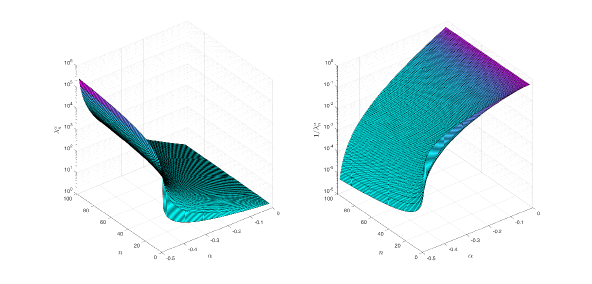
Figure 22: The surfaces of $\lambda_{n}^{\alpha}$ and its reciprocal on the discrete rectangular domain $\{(n,\alpha):n=1$:$100,\alpha=-0.49$:$0.0048$:$-0.01\}$.

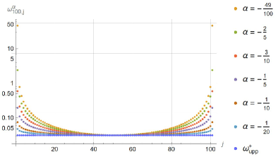
Figure 23: Plot of $\varpi_{100,j}^{\alpha}$ for $(j,\alpha)\in\mathbb{J}_{100}\times\{-0.49,-0.4:0.1:-0.1,-0.05\}$.

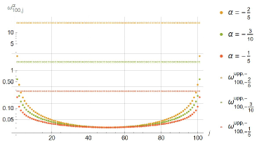
Figure 24: Plots of $\varpi_{100,j}^{\alpha}$ and $\varpi_{100,\alpha}^{\text{upp},-}$ for $(j,\alpha)\in\mathbb{J}_{100}\times\{-0.4:0.1:-0.2\}$.

The following two theorems highlight the stability of TG interpolation for $\alpha\in\,\mathbb{R}_{-1/2}^{-}$ using several space norms.

Theorem B.4.

$\,\forall_{\mkern-6.0mua}\,u\in L_{w_{i}^{\alpha,L}}^{2}\left(\mathbb{R}_{0}^{+}\right)$, we have

$${\left\|{I_{n}}u\right\|_{L_{w_{i}^{\alpha,L}}^{2}\left(\mathbb{R}_{0}^{+}\right)}}<\frac{\Gamma(\alpha+1/2)}{\sqrt{2}\,n^{1/2+\alpha}}\,{\left\|u\right\|_{L^{\infty}\left(\mathbb{R}_{0}^{+}\right)}}\quad\forall(n,\alpha,L,i)\in\,\mathrel{\mathop{\mathbb{Z}^{+}}\limits^{\vbox to0.0pt{\kern-2.0pt\hbox{$\scriptstyle\rightarrow$}\vss}}}\times\mathbb{R}_{-1/2}^{-}\times\mathbb{R}^{+}\times\mathbb{N}_{2}.$$ (B.23)

Proof.

The proof follows readily by Formula (B.11) and Lemma B.2. ∎

Theorem B.5.

$\,\forall_{\mkern-6.0mua}\,u\in H^{1}_{w_{i}^{\alpha,L}}\left(\mathbb{R}_{0}^{+}\right)\,\exists\,c\in\mathbb{R}^{+}:$

$${\left\|{I_{n}}u\right\|_{L_{w_{i}^{\alpha,L}}^{2}\left(\mathbb{R}_{0}^{+}\right)}}<c\,\Gamma(\alpha+1/2)\sqrt{\frac{n+1}{n^{1+2\alpha}}}\left({\left\|u\right\|_{L_{w_{i}^{\alpha,L}}^{2}\left(\mathbb{R}_{0}^{+}\right)}}+\frac{1}{n}\left\|\sqrt{(t+1)\sqrt{t}}\,u^{\prime}\right\|_{L^{2}\left(\mathbb{R}_{0}^{+}\right)}\right)\quad\forall(n,\alpha,L,i)\in\,\mathrel{\mathop{\mathbb{Z}^{+}}\limits^{\vbox to0.0pt{\kern-2.0pt\hbox{$\scriptstyle\rightarrow$}\vss}}}\times\mathbb{R}_{-1/2}^{-}\times\mathbb{R}^{+}\times\mathbb{N}_{2}.$$ (B.24)

Proof.

By closely following the proof of Theorem B.3, we have

$${\left\|{I_{n}}u\right\|_{L_{w_{i}^{\alpha,L}}^{2}\left(\mathbb{R}_{0}^{+}\right)}^{2}} <\varpi_{n,\alpha}^{\text{upp},-}\sum_{j\in\mathbb{J}_{n}}{\mathop{\sup}\limits_{\theta\in\mathscr{K}_{n,j}}\hat{u}^{2}(\theta)}\quad\forall(n,\alpha,L,i)\in\,\mathrel{\mathop{\mathbb{Z}^{+}}\limits^{\vbox to0.0pt{\kern-2.0pt\hbox{$\scriptstyle\rightarrow$}\vss}}}\times\mathbb{R}_{0}^{+}\times\mathbb{R}^{+}\times\mathbb{N}_{2}.$$ (B.25)

$$\Rightarrow\frac{2\pi n^{1+2\alpha}}{(n+1)\Gamma^{2}(\alpha+1/2)}{\left\|{I_{n}}u\right\|_{L_{w_{i}^{\alpha,L}}^{2}\left(\mathbb{R}_{0}^{+}\right)}^{2}} <\frac{\pi}{n+1}\sum_{j\in\mathbb{J}_{n}}{\mathop{\sup}\limits_{\theta\in\mathscr{K}_{n,j}}\hat{u}^{2}(\theta)}$$ (B.26)

$$<c_{1}\left({\left\|u\right\|^{2}_{L_{w_{i}^{\alpha,L}}^{2}\left(\mathbb{R}_{0}^{+}\right)}}+\frac{1}{n^{2}}\left\|\sqrt{(t+1)\sqrt{t}}\,u^{\prime}\right\|^{2}_{L^{2}\left(\mathbb{R}_{0}^{+}\right)}\right)\quad\,\forall_{\mkern-6.0mus}\,c_{1}\in\mathbb{R}^{+},$$ (B.27)

by following the proof of [20, Theorem 4.1]. Therefore,

$$\frac{1}{\Gamma(\alpha+1/2)}\sqrt{\frac{2\pi n^{1+2\alpha}}{(n+1)}}{\left\|{I_{n}}u\right\|_{L_{w_{i}^{\alpha,L}}^{2}\left(\mathbb{R}_{0}^{+}\right)}}<c_{2}\left({\left\|u\right\|_{L_{w_{i}^{\alpha,L}}^{2}\left(\mathbb{R}_{0}^{+}\right)}}+\frac{1}{n}\left\|\sqrt{(t+1)\sqrt{t}}\,u^{\prime}\right\|_{L^{2}\left(\mathbb{R}_{0}^{+}\right)}\right)\quad\,\forall_{\mkern-6.0mus}\,c_{2}\in\mathbb{R}^{+},$$ (B.28)

whence the proof is established. ∎

Theorems B.4 and B.5 show that the TG interpolation is asymptotically unstable for $(n,\alpha)\in\,\mathrel{\mathop{\mathbb{Z}^{+}}\limits^{\vbox to0.0pt{\kern-2.0pt\hbox{$\scriptstyle\rightarrow$}\vss}}}\times\mathrel{\mathop{\mathbb{R}}\limits^{\vbox to0.0pt{\kern-2.0pt\hbox{$\scriptstyle\rightarrow$}\vss}}}_{-1/2}$, and the instability increases as $\alpha\to-1/2$.

Declarations

Competing Interests

The authors declare there is no conflict of interest.

Availability of Supporting Data

The authors declare that the data supporting the findings of this study are available within the article.

Ethical Approval and Consent to Participate and Publish

Not Applicable.

Human and Animal Ethics

Not Applicable.

Consent for Publication

Not Applicable.

Funding

The authors received no financial support for the research, authorship, and/or publication of this article.

Acknowledgment

Special thanks to Dr. Jihyoung Cha for sharing the initial conditions and calculated optimal cost function values of Problems 1 and 2 used in [2], which were not explicitly reported there.

References

- Ko and Bitmead [2007] S. Ko, R. R. Bitmead, Optimal control for linear systems with state equality constraints, Automatica 43 (2007) 1573–1582.
- Cha et al. [2019] J. Cha, S. Kang, S. Ko, Infinite horizon optimal output feedback control for linear systems with state equality constraints, International Journal of Aeronautical and Space Sciences 20 (2019) 483–492.
- Li et al. [2020] S. Li, Z. Lai, L. Jin, X. Yu, Diagonalized Gegenbauer rational spectral methods for second-and fourth-order problems on the whole line, Applied Numerical Mathematics 151 (2020) 494–516.
- Hajimohammadi et al. [2020] Z. Hajimohammadi, F. Baharifard, K. Parand, A new numerical learning approach to solve general Falkner–Skan model, Engineering with Computers (2020) 1–17.
- Baharifard et al. [2022] F. Baharifard, K. Parand, M. Rashidi, Novel solution for heat and mass transfer of a MHD micropolar fluid flow on a moving plate with suction and injection, Engineering with Computers (2022) 1–18.
- Parand et al. [2018] K. Parand, A. Bahramnezhad, H. Farahani, A numerical method based on rational Gegenbauer functions for solving boundary layer flow of a Powell–Eyring non-Newtonian fluid, Computational and Applied Mathematics 37 (2018) 6053–6075.
- Elgindy and Refat [2023] K. T. Elgindy, H. M. Refat, A direct integral pseudospectral method for solving a class of infinite-horizon optimal control problems using Gegenbauer polynomials and certain parametric maps, AIMS Mathematics 8 (2023) 3561–3605.
- Dahy and Elgindy [2022] S. A. Dahy, K. T. Elgindy, High-order numerical solution of viscous Burgers’ equation using an extended Cole–Hopf barycentric Gegenbauer integral pseudospectral method, International Journal of Computer Mathematics 99 (2022) 446–464.
- Elgindy [2018] K. T. Elgindy, Optimal control of a parabolic distributed parameter system using a fully exponentially convergent barycentric shifted Gegenbauer integral pseudospectral method, Journal of Industrial and Management Optimization 14 (2018) 473–496.
- Elgindy and Dahy [2018] K. T. Elgindy, S. A. Dahy, High-order numerical solution of viscous Burgers’ equation using a Cole-Hopf barycentric Gegenbauer integral pseudospectral method, Mathematical Methods in the Applied Sciences 41 (2018) 6226–6251.
- Dai et al. [2016] M. Dai, X. Yang, Y. He, et al., Integral form and equivalence proof of three pseudospectral optimal control methods, Control and Decision 6 (2016) 1123–1127.
- Greengard [1991] L. Greengard, Spectral integration and two-point boundary value problems, SIAM Journal on Numerical Analysis 28 (1991) 1071–1080.
- Driscoll [2010] T. A. Driscoll, Automatic spectral collocation for integral, integro-differential, and integrally reformulated differential equations, Journal of Computational Physics 229 (2010) 5980–5998.
- Elgindy [2023a] K. T. Elgindy, New optimal periodic control policy for the optimal periodic performance of a chemostat using a Fourier–Gegenbauer-based predictor-corrector method, Journal of Process Control 127 (2023a) 102995.
- Elgindy [2023b] K. T. Elgindy, Fourier-Gegenbauer pseudospectral method for solving periodic fractional optimal control problems, arXiv preprint arXiv:2304.04454 (2023b).
- Elgindy [2023c] K. T. Elgindy, Fourier-Gegenbauer pseudospectral method for solving time-dependent one-dimensional fractional partial differential equations with variable coefficients and periodic solutions, arXiv preprint arXiv:2304.14061 (2023c).
- Elgindy and Smith-Miles [2013a] K. T. Elgindy, K. A. Smith-Miles, Fast, accurate, and small-scale direct trajectory optimization using a Gegenbauer transcription method, Journal of Computational and Applied Mathematics 251 (2013a) 93–116.
- Elgindy and Smith-Miles [2013b] K. T. Elgindy, K. A. Smith-Miles, Optimal Gegenbauer quadrature over arbitrary integration nodes, Journal of Computational and Applied Mathematics 242 (2013b) 82–106.
- Förster and Petras [1990] K.-J. Förster, K. Petras, On estimates for the weights in Gaussian quadrature in the ultraspherical case, Mathematics of computation 55 (1990) 243–264.
- Guo et al. [2002] B.-y. Guo, J. Shen, Z.-q. Wang, Chebyshev rational spectral and pseudospectral methods on a semi-infinite interval, International journal for numerical methods in engineering 53 (2002) 65–84.
- Elgindy and Smith-Miles [2013] K. T. Elgindy, K. A. Smith-Miles, Solving boundary value problems, integral, and integro-differential equations using Gegenbauer integration matrices, Journal of Computational and Applied Mathematics 237 (2013) 307–325.