Caterpillar: A Pure-MLP Architecture with Shifted-Pillars-Concatenation

Abstract

Modeling in Computer Vision has evolved to MLPs. Vision MLPs naturally lack local modeling capability, to which the simplest treatment is combined with convolutional layers. Convolution, famous for its sliding window scheme, also suffers from this scheme of redundancy and low computational efficiency. In this paper, we seek to dispense with the windowing scheme and introduce a more elaborate and effective approach to exploiting locality. To this end, we propose a new MLP module, namely Shifted-Pillars-Concatenation (SPC), that consists of two steps of processes: (1) Pillars-Shift, which generates four neighboring maps by shifting the input image along four directions, and (2) Pillars-Concatenation, which applies linear transformations and concatenation on the maps to aggregate local features. SPC module offers superior local modeling power and performance gains, making it a promising alternative to the convolutional layer. Then, we build a pure-MLP architecture called Caterpillar by replacing the convolutional layer with the SPC module in a hybrid model of sMLPNet [32]. Extensive experiments show Caterpillar’s excellent performance and scalability on both ImageNet-1K and small-scale classification benchmarks.

1 Introduction

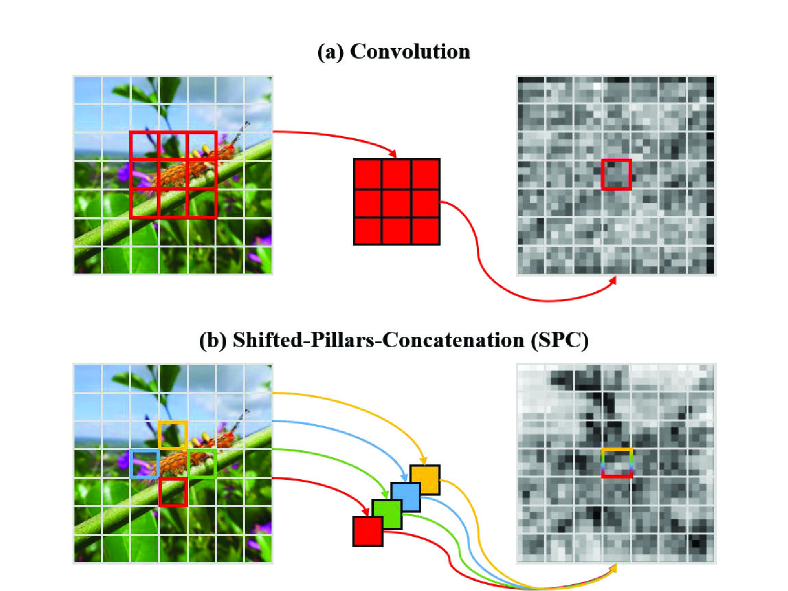
Figure 1: (a) The convolutional layer sequentially slides a local window with a larger receptive field, which can lead to low computational efficiency and redundant representation. (b) The proposed SPC module adopts a window-free strategy. It applies four linear filters that simultaneously encode the local features from the neighbors of four directions, exploiting the locality more elaborately and effectively.

Deep architectures in computer vision have evolved from Convolutional Neural Networks (CNNs), through Vision Transformers (ViTs), and now to Multi-Layer Perceptrons (MLPs). CNNs [20, 31, 13] primarily utilize convolution to aggregate local features but struggle to capture global dependencies between long-range pillars (tokens) in an image. ViTs [8, 35] employ self-attention mechanism to consider all pillars from a global perspective. Unfortunately, the self-attention mechanism suffers from high computational complexity. To overcome this weakness, MLP-based models [34] replace the self-attention layers with simple MLPs to perform token(spatial)-mixing across the input pillars, thereby significantly reducing the computational costs. However, early MLP models [34, 36] encountered the challenges in sufficiently incorporating local dependencies. As a solution, researchers have proposed hybrid models [32, 24] that combine convolutional layers with MLPs to achieve a balance between capturing local and global information, bringing stable performance improvements.

Convolutional layers slide a local window across an image to introduce locality and translation-invariance, which have brought great successes for CNNs [20, 13] and also inspired a number of influential ViTs [43, 28]. Nevertheless, convolution has inherent drawbacks. First, it may introduce redundancy, especially to the edge features. The convolution aggregates pixels in a local window with a larger receptive scope, while the edge features, such as shape and contour, often consist of only a few pixels that cannot fully fill the scope. Therefore, the edges can obtain mixed information with the background, leading to redundant representation. Additionally, the sliding window needs to encode features sequentially and individually in each position. This sequential nature limits the parallel computing capability and causes lower computational efficiency.

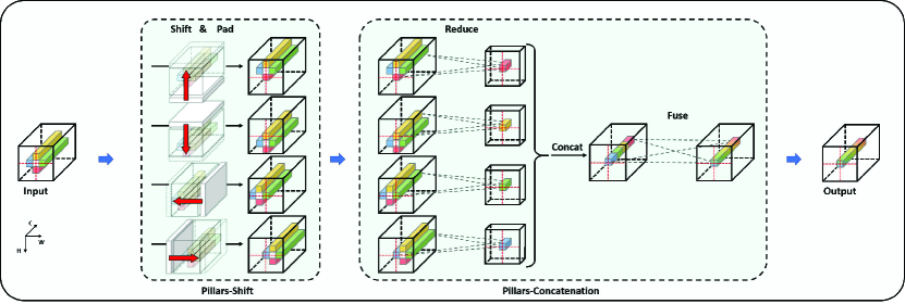
Figure 2: The SPC module consists of two processes: Pillars-Shift (Shift + Pad) and Pillars-Concatenation (Reduce + Concat + Fuse). In Pillars-Shift, the input image is recurrently shifted along four directions to create neighboring maps, while Pad is used to maintain the feature size by padding these maps with pillars of specific values. In Pillars-Concatenation, Reduce is achieved through four C $\times$ C/4 linear projections, and Fuse is accomplished through a C $\times$ C linear projection, where C represents the number of input feature channels.

In this paper, we seek to break the sequential windowing scheme and present an alternative to convolution. To this end, we propose a new MLP-based module called Shifted-Pillars-Concatenation (SPC) that consists of two processes: Pillars-Shift and Pillars-Concatenation. In Pillars-Shift, we shift the input image along four directions (i.e., up, down, left, right) to create four neighboring maps, with the local information for all pillars decomposed into four respective groups according to the orientation of neighboring pillars. In Pillars-Concatenation, we apply four linear transformations to individually encode these maps of discrete groups and then concatenate them together, with each pillar achieving the simultaneous and elaborate aggregation of local information from its four neighbors. Based on the proposed SPC, we introduce a pure-MLP architecture namely Caterpillar, which is built by replacing the (depth-wise) convolutional layer with the proposed SPC module in a Conv-MLP hybrid model (i.e., sMLPNet[32]). The Caterpillar inherits the advantages of sMLPNet, which clearly separates the local- and global-mixing operations in its spatial-mixing blocks and utilizes the sparse-MLP (sMLP) layer to aggregate global features (Figure 3, left), while leveraging the SPC module to exploit locality.

For experiments, we uniformly validate the direct application of the Caterpillar with various vision architectures (i.e., CNNs, ViTs, MLPs, Hybrid models) on common-used small-scale images [39, 19, 44], among which the Caterpillar achieves the best performance on all used datasets. On the popular ImageNet-1K benchmark, the Caterpillar series attains better or comparable performance to recent state-of-the-art methods (e.g., Caterpillar-B, 83.7%). On the other hand, in all experiments, the Caterpillars obtain higher accuracy than the baseline sMLPNets, while changing the convolution to the SPC module in ResNet-18 brings 4.7% top-1 accuracy gains on ImageNet-1K dataset, demonstrating the potential of SPC to serve as an alternative to convolution in both plug-and-play and independent ways.

In summary, the major contributions of this paper are listed as follows:

• We propose a new SPC module that can capture local information in a window-free scheme, and prove its potential to serve as an alternative to convolutional layers.

• We construct a new pure-MLP model called Caterpillar that separately captures the local and global information for feature learning.

• Extensive experiments on small- and large-scale popular datasets demonstrate the superior or comparable performance of the Caterpillar to recent state-of-the-art methods, with better performance of SPC than convolution.

2 Related Work

2.1 Local Modeling Approaches

The idea of local modeling can be traced back to research on the organization of the visual cortex [16, 17], which inspired Fukushima to introduce the Cognitron [9], a neural architecture that models nearby features in local regions. Departing from biological inspiration, Fukushima further proposed Neocognitron [10], which introduces weight sharing across spatial locations through a sliding window strategy. LeCun combined weight sharing with back-propagation algorithm and introduced LeNet [23, 21, 22], laying the foundation for the widespread adoption of CNNs in the Deep Learning era. Since 2012, when AlexNet [20] achieved remarkable performance in the ImageNet classification competition, convolution-based methods have dominated the field of computer vision for nearly a decade. With the popularity of CNNs, research efforts have been devoted to improving individual convolutional layers, such as depth-wise convolution [45] and deformable convolution [6]. On the other hand, alternative approaches to replace convolution have also been explored, such as the shift-based methods involving sparse-shift [3] and partial-shift [26]. The idea behind these approaches is to move each channel of the input image in different spatial directions, and mix spatial information through linear transformations across channels. The proposed SPC module also builds upon the shift idea but shifts the entire image into four neighboring maps in the process of Pillars-Shift, while making use of the linear projections and concatenation in Pillars-Concatenation.

2.2 Neural Architectures for Vision

CNNs and Vision Transformers. CNNs have achieved remarkable success in computer vision, with well-known models including AlexNet [20], VGG [31] and ResNet [13]. The attention-based Transformer, initially proposed for machine translation [38], has been successfully applied to vision tasks with the introduction of Vision Transformer (ViT) [8]. Since then, various advancements have been proposed to improve training efficiency and model performance for ViTs, such as data-efficient training strategy [35] and pyramid architecture [40, 28], which have also benefited the entire vision field. At the core of Transformer models lies the multi-head self-attention mechanism. The proposed SPC module shares similar operation to the multi-head settings, as it encodes local neighboring information from different representation subspaces with multiple linear filters in the Pillars-Concatenation process.

Vision MLPs. Vision MLPs [34, 36, 2, 11, 33, 15, 41, 47, 46, 25] have also made significant progress since the invention of MLP-Mixer [34], which pioneer to interleave the token-mixing (cross-location) operations and channel-mixing (per-location) operations to aggregate spatial and channel information, respectively. Early MLP-based models, such as MLP-Mixer [34] and ResMLP [36], perform token-mixing across all pillars from a global perspective, lacking the ability to effectively model local features. As a result, a number of studies propose to enhance MLPs with local modeling capabilities. HireMLP [11], for instance, introduces inner-region rearrangement to aggregate local features, while AS-MLP [25] adopts an axial-shift strategy. For the Caterpillar, it incorporates local information through the proposed SPC module.

Hybrid Architectures. In addition to the MLP methods which capture both local and global dependencies in parallel [11], research that augment MLPs with convolutional layers to separately aggregate these two types of information have also been conducted [24, 32, 1]. Among them, sMLPNet [32] introduces a sparse-MLP module to aggregate global information while using the depth-wise convolutional (DWConv) layer to model local features. Concurrent with our work, Strip-MLP [1] chiefly replaces the sparse-MLP (i.e., the global-mixing module) in sMLPNet with a Strip-MLP layer, achieving superior scores on both large- and small-scale image datasets. The proposed Caterpillar is also built upon the sMLPNet but replaces the DWConv (i.e., the local-mixing module) with the SPC module, leading to a pure-MLP architecture that also attains excellent performance on various-scale image recognition tasks.

3 Method

3.1 Shifted-Pillars-Concatenation Module

In this section, we first introduce the SPC module, of which the working procedure can be decomposed into Pillars-Shift and Pillars-Concatenation, as shown in Figure 2. Then, we analyze its computational parameters with that of the standard and depth-wise convolutional layers.

3.1.1 Shifted-Pillars-Concatenation

Pillars-Shift. This process is to shift and pad an input image into four neighboring maps, which can be formed as:

$$\begin{array}[]{cc}\mathrm{PS}\left(\mathbf{X}\mid dir,s,p_{m}\right)=\mathrm{Pad}\left(\mathrm{Shift}\left(\mathbf{X},dir,s\right),p_{m}\right),&\\ dir\subseteq\mathcal{D}_{s},\end{array}$$ (3)

where $dir$, $s$ and $p_{m}$ denote the shifting direction, shifting steps and padding mode, respectively. $\mathcal{D}_{s}$ is a set which contains shifting directions.

Specifically, let $\mathbf{x}_{ij}\in\mathbb{R}^{C}$ represent a feature vector (pillar), we can have an image:

$$\mathbf{X}_{in}=\left[\begin{matrix}\mathbf{x}_{11}&\mathbf{x}_{12}&\cdots&\mathbf{x}_{1W}\\ \ \mathbf{x}_{21}&\mathbf{x}_{22}&\cdots&\mathbf{x}_{2W}\\ \ \vdots&\vdots&\vdots&\vdots\\ \ \mathbf{x}_{(H-1)1}&\mathbf{x}_{(H-1)2}&\cdots&\mathbf{x}_{(H-1)W}\\ \ \mathbf{x}_{H1}&\mathbf{x}_{H2}&\cdots&\mathbf{x}_{HW}\end{matrix}\right],$$

which means $\mathbf{X}_{in}\in\mathbb{R}^{H\times W\times C}$, where $H$, $W$ and $C$ represent the width, height and channel number, respectively. Taking $\mathbf{X}_{u}$ (i.e., the up-wise neighboring map) as an example, we first perform a shift operation on $\mathbf{X}_{in}$ by setting $dir$=$`up^{\prime}$ and $s=1$, so that $\mathbf{X}_{in}$ is transformed to:

$$\mathbf{X}^{{}^{\prime}}_{\mathit{u}}=\left[\begin{matrix}\mathbf{x}_{21}&\mathbf{x}_{22}&\cdots&\mathbf{x}_{2W}\\ \ \vdots&\vdots&\vdots&\vdots\\ \ \mathbf{x}_{(H-1)1}&\mathbf{x}_{(H-1)2}&\cdots&\mathbf{x}_{(H-1)W}\\ \ \mathbf{x}_{H1}&\mathbf{x}_{H2}&\cdots&\mathbf{x}_{HW}\\ \ \end{matrix}\right],$$

where $\mathbf{X}^{\prime}_{\mathit{u}}\in\mathbb{R}^{(H-1)\times W\times C}$. Then, we pad $\mathbf{X}^{{}^{\prime}}_{\mathit{u}}$ according to the Zero Padding and attain the $\mathbf{X}_{u}$:

$$\mathbf{X}_{\mathit{u}}=\left[\begin{matrix}\mathbf{x}_{21}&\mathbf{x}_{22}&\cdots&\mathbf{x}_{2W}\\ \ \vdots&\vdots&\vdots\\ \ \mathbf{x}_{(H-1)1}&\mathbf{x}_{(H-1)2}&\cdots&\mathbf{x}_{(H-1)W}\\ \ \mathbf{x}_{H1}&\mathbf{x}_{H2}&\cdots&\mathbf{x}_{HW}\\ \ \mathbf{0}&\mathbf{0}&\cdots&\mathbf{0}\end{matrix}\right],$$

where $\mathbf{X}_{\mathit{u}}\in\mathbb{R}^{H\times W\times C}$. By default settings with $\mathcal{D}_{s}$ of $\left[`up^{\prime},`down^{\prime},`left^{\prime},`right^{\prime}\right]$, the input $\mathbf{X}_{in}$ will be transformed into four neighboring maps of $\mathbf{X}_{u},\mathbf{X}_{d},\mathbf{X}_{l},\mathbf{X}_{r}$, where $\mathbf{X}_{\mathit{d}},\mathbf{X}_{\mathit{l}},\mathbf{X}_{\mathit{r}}\in\mathbb{R}^{H\times W\times C}$.

Pillars-Concatenation. Obviously, Pillars-Shift has no parameter learning, which would weaken the representation capability of the module. To overcome this deficiency, we introduce the Pillars-Concatenation process. Specifically, the neighboring maps $\mathbf{X}_{u},\mathbf{X}_{d},\mathbf{X}_{l},\mathbf{X}_{r}$ are projected through four independent fully-connected (FC) layers. The parameters are $\mathbf{W}_{u},\mathbf{W}_{d},\mathbf{W}_{l},\mathbf{W}_{r}\in\mathbb{R}^{C\times C/4}$, respectively, so as to reduce the number of neighboring maps’ channels to $C/4$. After that, all of the reduced maps are concatenated along the channel dimension and then projected again, by an FC layer with the parameters $\mathbf{W}\in\mathbb{R}^{C\times C}$ to fuse the local features. This process can be represented as:

$$\mathrm{PC}\left(\mathbf{X}\right)=\mathrm{Concat}\left(\mathbf{X}_{u}\mathbf{W}_{u},\mathbf{X}_{d}\mathbf{W}_{d},\mathbf{X}_{l}\mathbf{W}_{l},\mathbf{X}_{r}\mathbf{W}_{r}\right)\mathbf{W},$$ (4)

Through the Pillars-Concatenation, the four neighboring maps are reduced, concatenated and finally fused into the $\mathbf{X}_{out}\in\mathbb{R}^{H\times W\times C}$, with the local information for all pillars within the image aggregated in parallel.

3.1.2 Parameter Analysis with Convolutions

For an input image with the input dimension of $d_{in}$ and output dimension of $d_{out}$, the number of parameters in standard and depth-wise convolution can be calculated as $d_{in}\times k^{2}\times d_{out}$ and $d_{in}\times k^{2}$, respectively, with $k$ representing the kernel size. In comparison, The parameters of SPC module are $d_{in}\times d_{in}+d_{in}\times d_{out}$ (detailed as $d_{in}\times d_{in}/4\times 4+d_{in}\times d_{out}$). In the typical scenario where $d_{in}$ is equal to $d_{out}$, the parameters of a standard 3 $\times$ 3 convolution are $9\times{d_{in}}^{2}$, which is 4.5 times larger than that of SPC, i.e., $2\times{d_{in}}^{2}$, demonstrating that the SPC module has lower computational complexity than the standard convolutional layers. Additionally, the parameters in the 3 $\times$ 3 depth-wise convolution (adapted in sMLPNet) are $9\times d_{in}$.

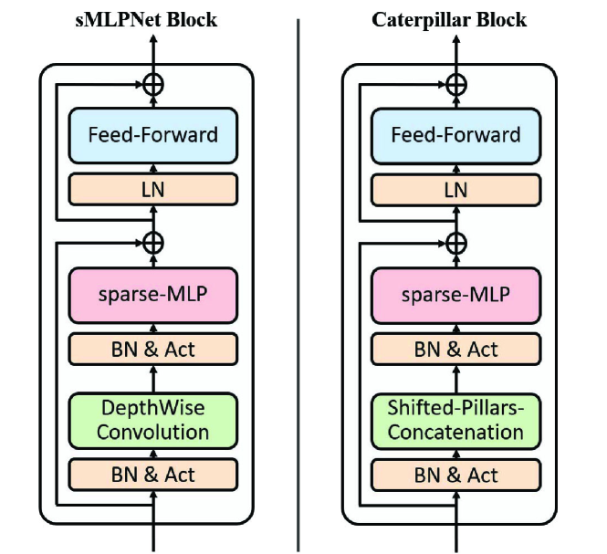
Figure 3: The structures of sMLPNet and Caterpillar blocks.

3.2 Caterpillar Block

Caterpillar block is built by replacing the depth-wise convolution with the SPC module in sMLPNet block [32], in which a sparse-MLP (sMLP) module (illustrated in Supplementary F) is introduced for aggregating global features. As illustrated in Figure 3, a Caterpillar block contains three basic modules: an SPC module and an sMLP module, with a BatchNorm (BN) and a GELU nonlinearity applied before them, and a FFN module, with following a LayerNorm (LN) layer. The SPC and sMLP form the token-mixing component and the FFN servers as channel-mixing module, with applied two residual connections.

Given an image $\mathbf{X}\in\mathbb{R}^{H\times W\times C}$, the calculation in the Caterpillar block can be formulated as:

$$\mathbf{X}^{\prime}=\mathrm{GELU}\left(\mathrm{BN}\left(\mathrm{SPC}\left(\mathbf{X})\right)\right)\right),$$ (5)

$$\mathbf{Y}=\mathrm{GELU}\left(\mathrm{BN}\left(\mathrm{sMLP}\left(\mathbf{X}^{\prime})\right)\right)\right)+\mathbf{X},$$ (6)

$$\mathbf{Z}=\mathrm{LN}\left(\mathrm{FFN}\left(\mathbf{Y})\right)\right)+\mathbf{Y},$$ (7)

where $\mathbf{X}^{\prime}$ denotes the output features of the SPC layer, $\mathbf{Y}$ and $\mathbf{Z}$ represent the output of token-mixing and channel-mixing modules, respectively.

3.3 Caterpillar Architectures

We build the Caterpillar architectures in a pyramid structure of four stages, which first represent the input images into patch-level features, and gradually shrink the spatial size of the feature maps as the network deepens. This enables Caterpillar to leverage the scale-invariant property of images as well as make full use of multi-scale features.

We introduce five variants of Caterpillar architectures, i.e., Caterpillar-Mi, -Tx, -T, -S and -B, with different numbers of Caterpillar blocks stacked in their four stages. The architecture hyper-parameters of these variants are:

• Caterpillar-Mi: $C$ = 40, layer numbers = {2,6,10,2}

• Caterpillar-Tx: $C$ = 60, layer numbers = {2,8,14,2}

• Caterpillar-T: $C$ = 80, layer numbers = {2,8,14,2}

• Caterpillar-S: $C$ = 96, layer numbers = {2,10,24,2}

• Caterpillar-B: $C$ = 112, layer numbers = {2,10,24,2}

where $C$ is the channel number of the hidden layers in the first stage, and layer numbers denote the number of blocks in each of their four stages. Detailed configurations can be found in Supplementary C.

4 Experiments

In this Section, we organize the experiments as follows: We compare the direct application of Caterpillar with various vision models on small-scale images in Section 4.1. Then, we test the Caterpillar on the ImageNet-1K dataset in Section 4.2. After that, we conduct ablation studies in Section 4.3, followed by the visualization analysis for SPC in Section 4.4. Finally, in Section 4.5, we further explore the application of SPC to replace convolution in ResNet(-18).

4.1 Small-scale Images Classification

Datasets. We conduct small-scale image recognition experiments on four commonly-used benchmarks: Mini-ImageNet (MIN) [39], CIFAR-10 (C10) [19], CIFAR-100 (C100) [19] and Fashion-MNIST (Fashion) [44]. We utilize these images in their original sizes, different from the settings in [1] which resized images into 224 $\times$ 224.

Experimental Settings. We evaluate the Caterpillar with fourteen representative vision models, including six MLP models [36, 2, 11, 33, 15, 41], two CNN models [13, 37], three Transformer models [35, 28, 50], and three hybrid models [12, 32, 1], as tagged in Table 1. All models are directly trained on the small images without extra data. To enable the models adaptable to small-sized images (e.g., 32 $\times$ 32), we change their patch embedding layers into small patch sizes according to uniform rules, of which the detailed implementation is provided in Supplemental D. For a fair comparison, we adopt the same training strategies that were presented in their original papers (for ImageNet-1K), which are presented in Supplemental E.

Table 1: Results (%) of Caterpillar and other MLP / CNN / Transformer / Hybrid vision models on four small-scale datasets. As the model parameters and FLOPs are similar on these datasets, we just report those metrics on CIFAR-10 for clarity. The result of CCT-7/3×1 on MIN is omitted, since the FLOPs of it (i.e., 6.6G) is much larger than that of other models. The Caterpillar-T^† scales the number of channels to [72, 144, 288, 576], with similar computational costs to the sMLPNet-T. $\blacktriangle$ CNN, $\blacklozenge$ Transformer, $\blacksquare$ MLP, $\blacksquare$ Hybrid, $\bigstar$ Ours.

Networks	MIN	C10	C100	Fashion	Params	FLOPs
$\blacklozenge$ DeiT-Ti	54.55	88.87	67.46	92.97	5.4M	0.3G
$\blacklozenge$ NesT-T	73.44	94.05	75.60	94.26	6.4M	2.3G
$\blacksquare$ CCT-7/3×1	–	91.80	74.09	93.70	3.7M	0.9G
$\bigstar$ Caterpillar-Mi	74.14	95.54	79.41	95.14	5.9M	0.4G
$\blacktriangle$ ResNet-18	70.95	95.54	77.66	95.11	11.2M	0.7G
$\blacktriangle$ ConvMixer_768/32	57.94	91.54	70.13	93.36	19.4M	1.2G
$\blacksquare$ ResMLP-S12	68.63	93.67	76.44	94.58	14.3M	0.9G
$\blacksquare$ CycleMLP-B1	70.68	88.06	66.17	92.87	12.7M	0.1G
$\blacksquare$ HireMLP-Tiny	71.66	86.42	62.13	92.35	17.6M	0.1G
$\blacksquare$ Wave-MLP-T	72.15	88.85	65.92	92.83	16.7M	0.1G
$\blacksquare$ Strip-MLP-T*	76.05	96.34	82.53	95.33	16.3M	0.8G
$\bigstar$ Caterpillar-Tx	77.27	96.54	82.69	95.38	16.0M	1.1G
$\blacktriangle$ ResNet-34	72.03	95.92	79.53	95.48	21.3M	1.5G
$\blacktriangle$ ResNet-50	72.65	96.06	79.11	95.28	23.7M	1.6G
$\blacklozenge$ DeiT-S	42.41	83.10	64.65	93.43	21.4M	1.4G
$\blacklozenge$ Swin-T	53.11	85.69	67.60	89.90	27.6M	1.4G
$\blacksquare$ ResMLP-S24	69.63	94.76	78.65	95.27	28.5M	1.9G
$\blacksquare$ CycleMLP-B2	71.11	88.84	67.83	93.41	22.6M	0.1G
$\blacksquare$ HireMLP-Small	73.86	88.51	62.54	92.70	32.6M	0.1G
$\blacksquare$ Wave-MLP-S	67.51	88.37	63.24	92.96	30.2M	0.1G
$\blacksquare$ ViP-Small/7	70.94	94.12	78.28	95.22	24.7M	1.7G
$\blacksquare$ DynaMixer-S	71.40	95.32	78.34	95.14	25.2M	1.8G
$\blacksquare$ sMLPNet-T	77.07	96.87	82.89	95.53	23.5M	1.6G
$\blacksquare$ Strip-MLP-T	76.47	96.48	82.59	95.50	22.5M	1.2G
$\bigstar$ Caterpillar-T†	77.56	97.08	83.12	95.57	23.0M	1.6G
$\bigstar$ Caterpillar-T	78.16	97.10	83.86	95.72	28.4M	1.9G
$\bigstar$ Caterpillar-S	78.94	97.22	84.40	95.80	58.0M	4.1G
$\bigstar$ Caterpillar-B	79.06	97.35	84.77	95.85	78.8M	5.5G

Results. From Table 1, our Caterpillar outperforms the sMLPNet on all four benchmarks, showcasing the better classification capability of the SPC than convolutional layers and its potential to be an alternative to convolution in plug-and-play ways. Additionally, the proposed Caterpillars attain the best scores among all tested architectures, e.g., the Caterpillar-T reaches 78.16% accuracy on MIN, 97.10% on C10, 84.86% on C100, and 95.72% on Fashion.

Scalability analysis. “Simple algorithms that scale well are the core of deep learning” [14]. Thus, we scale the Caterpillar from -Mi with FLOPs about 0.4G to -B about 5.5G, i.e., Caterpillar-Mi, -Tx, -T, -S and -B. It is credible that Caterpillar possesses excellent scalability on small-scale datasets, as it obtains steady improvement from bigger models.

4.2 ImageNet Classification

Datasets. We test the Caterpillar on ImageNet-1K benchmark [7], which consists of 1.28M training and 50K validation images belonging to 1,000 categories.

Experimental Settings. We train our models on 8 NVIDIA GeForce RTX 3090 GPUs with gradient accumulation techniques. For training strategies, we employ the AdamW [29] optimizer to train our models for 300 epochs, with a weight decay of 0.05 and a batch size of 1024. The learning rate is initially 1e-3 and gradually drops to 1e-5 according to the consine schedule. The data augmentation includes Random Augment [5], Mixup [49], Cutmix [48], Random Erasing [51]. More details are shown in Supplemental E.

Table 2: Results (%) of Caterpillar and other vision models on ImageNet-1K datasets. $\blacktriangle$ CNN, $\blacklozenge$ Transformer, $\blacksquare$ MLP, $\blacksquare$ Hybrid, $\bigstar$ Ours.

Networks	Params	FLOPs	Top-1
$\blacklozenge$ DeiT-Ti[35]	5M	1.1G	72.2
$\blacksquare$ gMLP-Ti[27]	6M	1.4G	72.3
$\bigstar$ Caterpillar-Mi	6M	1.2G	76.3
$\blacktriangle$ ResNet-18[13, 42]	12M	1.8G	70.6
$\blacksquare$ ResMLP-S12[36]	15M	3.0G	76.6
$\blacksquare$ Hire-MLP-Ti[11]	18M	2.1G	79.7
$\blacksquare$ Strip-MLP-T*[1]	18M	2.5G	81.2
$\bigstar$ Caterpillar-Tx	16M	3.4G	80.9
$\blacktriangle$ ResNet-50[13, 42]	26M	4.1G	79.8
$\blacktriangle$ RegNetY-4G[30]	21M	4.0G	80.0
$\blacklozenge$ DeiT-S[35]	22M	4.6G	79.8
$\blacklozenge$ Swin-T[28]	29M	4.5G	81.3
$\blacksquare$ ResMLP-S24[36]	30M	6.0G	79.4
$\blacksquare$ ViP-Small/7[15]	25M	6.9G	81.5
$\blacksquare$ Hire-MLP-S[11]	33M	4.2G	82.1
$\blacksquare$ CCT-14/7$\times$2[12]	22M	5.5G	80.7
$\blacksquare$ sMLPNet-T[32]	24M	5.0G	81.9
$\blacksquare$ Strip-MLP-T[1]	25M	3.7G	82.2
$\bigstar$ Caterpillar-T	29M	6.0G	82.4
$\blacktriangle$ ResNet-101[13, 42]	45M	7.9G	81.3
$\blacktriangle$ RegNetY-8G[30]	39M	8.0G	81.7
$\blacklozenge$ Swin-S[28]	50M	8.7G	83.0
$\blacksquare$ ViP-Medium/7[15]	55M	16.3G	82.7
$\blacksquare$ Hire-MLP-B[11]	58M	8.1G	83.2
$\blacksquare$ sMLPNet-S[32]	49M	10.3G	83.1
$\blacksquare$ Strip-MLP-S[1]	44M	6.8G	83.3
$\bigstar$ Caterpillar-S	60M	12.5G	83.5
$\blacktriangle$ ResNet-152[13, 42]	60M	11.6G	81.8
$\blacktriangle$ RegNetY-16G[30]	84M	16.0G	82.9
$\blacklozenge$ DeiT-B[35]	86M	17.5G	81.8
$\blacklozenge$ Swin-B[28]	88M	15.4G	83.5
$\blacksquare$ ResMLP-B24[36]	116M	23.0G	81.0
$\blacksquare$ ViP-Large/7[15]	88M	24.4G	83.2
$\blacksquare$ Hire-MLP-B[11]	96M	13.4G	83.8
$\blacksquare$ sMLPNet-B[32]	66M	14.0G	83.4
$\blacksquare$ Strip-MLP-B[1]	57M	9.2G	83.6
$\bigstar$ Caterpillar-B	80M	17.0G	83.7

Results. Table 2 presents the performance of Caterpillar with other well-established methods on ImageNet-1k benchmark. Similar to the results in Section 4.1, the Caterpillar models consistently outperform their sMLPNet counterparts, which further emphasizes the superiority of the SPC module over convolutional layers, highlighting its potential as a plug-and-play replacement to convolution. Furthermore, Caterpillar series reach competitive or even superior performance to state-of-the-art networks. For example, Caterpillar-B achieves the top-1 accuracy of 83.7%, indicating that Caterpillar is also capable of handling large-scale vision recognition tasks.

4.3 Ablation Study

In this section, we ablate essential design components in the proposed Caterpillar architecture. We use the same datasets and experimental settings as in Section 4.1. The base architecture is Caterpillar-T.

4.3.1 Pillars-Shift of SPC

Number of shift directions. This hyper-parameter ($N_{D}$) controls the shifting directions of input images so as to determine the receptive field of SPC on local features. We experiment with $N_{D}$ values ranging from 4 to 9. Among them, 4 represents the scope of four neighboring directions (up, down, left, and right), and 5 includes the center pillar itself. 8 covers a wider scope, including up, down, left, right, up-left, up-right, down-left, and down-right directions. When $N_{D}$ is set to 9, it adds the center pillar itself, which is similar to the scope of 3x3 convolution. From Table 3, the best trade-off between computational costs and accuracy is achieved when $N_{D}=4$. This suggests that local features can be sufficiently obtained from a 4-scoped receptive field.

Table 3: Results (%) on different numbers of shift directions in the Pillars-Shift process. The model with $N_{D}$ of 9^∗ adopts the channel numbers of [81, 162, 324, 648] in its four stages.

Num. of dir. ($N_{D}$)	MIN	C10	C100	Fashion	Params	FLOPs
4	78.16	97.10	83.86	95.72	28.4M	1.9G
5	78.04	96.93	83.55	95.63	28.4M	1.9G
8	78.19	96.92	83.58	95.57	28.4M	1.9G
9∗	77.92	96.82	83.60	95.52	29.1M	2.0G

Number of shift steps. The hyper-parameter $s$ determines the range of local features for the Pillars-Shift operation. When $s$ is set to 0, 1, or 2, the input image is shifted 0, 1, or 2 steps along the corresponding directions, which allows the local information for each pillar to be aggregated from itself (no shifting), neighboring pillars (with a distance of 1), or distant pillars (with a distance of 2), respectively. Table 4 displays the results of the proposed method with different numbers of shifting steps. The findings indicate that the best performance is achieved when $s=1$.

Table 4: The model accuracy (%) on three different shift steps in the Pillars-Shift process.

shift steps ($s$)	MIN	C10	C100	Fashion
0	76.71	95.84	81.12	95.22
1	78.16	97.10	83.86	95.72
2	76.29	96.17	82.04	95.26

Type of padding modes. The padding operation is to supplement pillars to the tail in neighboring maps. Different modes can decide what noises (extra information) would be injected to the pillars on the margin of images. We test four popular padding modes in Table 5. Among them, Replicated Padding can inject repeated features to the marginal pillars, which might bring redundancy. Both the Circular and Reflect modes add long-distance information to those pillars, which is obviously detrimental to the locality bias. Zero Padding is clean and thus achieves the best accuracy.

Table 5: The model accuracy (%) on four different padding modes in the Pillars-Shift process.

Padding Mode ($p_{m}$)	MIN	C10	C100	Fashion
Zero	78.16	97.10	83.86	95.72
Replicated	78.13	96.88	83.35	95.41
Circular	78.08	96.81	83.40	95.45
Reflect	77.76	96.89	83.33	95.40

4.3.2 Pillars-Concatenation of SPC

The Pillars-Concatenation process involves three key operations: (1) Reduce, which enables diverse representation by transforming neighboring maps in multiple representation spaces; (2) Concatenation (Concat), which integrates four neighboring maps to combine local features for all pillars in parallel; and (3) Fuse, which selectively learns and weights neighboring features to enhance the representation capabilities. We ablate five combinations of these operations in Table 6 and observe that Reduce+Concat+Fuse and Concat+Fuse perform better than the other options. Among them, Reduce+Concat+Fuse achieves a better trade-off between computational costs and accuracy.

Table 6: Results (%) of different ways to mix local neighbors.

Mixing ways	MIN	C10	C100	Fashion	Params	FLOPs
Reduce+Concat+Fuse	78.16	97.10	83.86	95.72	28.4M	1.9G
Reduce+Concat	77.72	97.02	83.26	95.72	25.9M	1.8G
Concat+Fuse	78.37	97.06	83.94	95.45	33.3M	2.3G
Sum+Fuse	76.14	96.16	80.88	95.28	25.9M	1.8G
Sum	74.81	95.33	75.48	95.34	23.4M	1.6G

4.3.3 Local-Global Combination Strategies

In Section 4.1 and 4.2, the sMLPNet, Strip-MLP, and Caterpillar all attained excellent performance on both small- and large-scale image recognition tasks. This success could be attributed to the common strategy that they clearly separate the local- and global-mixing operations in their token-mixing modules. However, both the sMLPNet and Strip-MLP missed the experiments to further explore the effects of local-global combination ways. To fill this gap, we conduct this ablation and perform various strategies as depicted in Figure 4. We evaluate six strategies, denoted as (a), (b), (c) for sequential regimes, and (e), (f), (g) for parallel methods, by rearranging the SPC and sMLP modules in Caterpillar blocks. Table 7 shows that the simply sequential methods generally outperform the complicated parallel strategies. We attribute this phenomenon to the idea that the ‘High-Cohesion and Low-Coupling’ principle leads to higher performance, as the internal SPC and sMLP modules are both working in sophisticated parallel ways. Furthermore, the L-G strategy achieves the best performance.

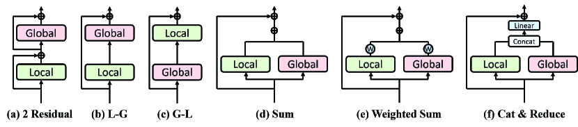
Figure 4: Different ways to combine local and global information.

Table 7: Comparison (%) between six different strategies for combining local and global information.

Combine ways	MIN	C10	C100	Fashion	Params	FLOPs
2 Residual	77.06	96.92	82.51	95.64	28.4M	1.9G
L-G (default)	78.16	97.10	83.86	95.72	28.4M	1.9G
G-L	78.09	96.88	83.45	95.65	28.4M	1.9G
Sum	76.91	96.70	82.13	95.53	28.4M	1.9G
Weighted Sum	77.94	96.82	82.56	95.60	30.3M	2.0G
Concat+Reduce	76.77	96.18	82.15	95.49	33.4M	2.3G

4.4 Visualization

To understand how the SPC module processes image data, we visualize the feature maps encoded by SPC coupled with two control ways. Specifically, we build three Caterpillar-T models with the local modules of identity, convolution and SPC, and implement them on the CIFAR-100 dataset. Figure 5 illustrates the feature maps of six samples, each of which is presented with 3 rows and 4 columns, where rows represent different local-mixing ways and columns are feature maps of different phases in models. For these samples, with the (a) cattle as an example, the patterns in SPC features are closer to the convolution and different from the identity. Since convolutional layers capably capture local features, the SPC is also capable of aggregating local information. Furthermore, compared to convolution, the objects in SPC maps exhibit more prominent edge features and are closer to the original input image, indicating that the proposed SPC module can encode local information more elaborately and avoid redundancy issues.

Figure 5: We display the feature maps of six samples with 3 rows and 4 columns. Each row represents a specific local modeling approach: identity (Iden.), convolution (Conv.) and SPC. The columns are maps in different phases of Caterpillar(CPr.)-T.

4.5 Exploration for SPC

Previous comparison between Caterpillars and sMLPNets demonstrates the potential of SPC as an alternative to convolution in plug-and-play ways. We further explore the SPC to serve as the main module for neural architectures.

Datasets. We utilize the same large-scale benchmark of ImageNet-1K as well as the small-scale datasets of MIN, C10, C100 and Fashion, as those in Section 4.1 and 4.2.

Experimental Settings. We adopt classic ResNet-18 (Res-18) [13] as the baseline CNN. Then, we replace the convolutional layers in Res-18’s basic blocks with the SPC module and obtain three SPC-based variants referred to as ‘Res-18(SPC)’, with $N_{C}$ utilized to adjust model complexity. For training these models, we follow the ‘Procedure A2’ in [42].

Results. Table 8 displays the ImageNet-1K classification results for the original Res-18 and Res-18(SPC) variants. As we can see, SPC can provide higher performance than convolution with only half of the parameters (Res-18(SPC), $N_{C}$=96). Increasing $N_{C}$ to 128, the Res-18(SPC) reaches similar computational costs to the baseline Res-18 while achieving 4.7% higher accuracy. Similar trends can be observed on small-scale recognition tasks, as shown in Supplementary A. These results confirm that the SPC module can also be used as the main component to construct neural networks, potentially serving as an alternative to convolutional layers in independent manners.

Table 8: Results (%) of Res-18 and Res-18(SPC) on ImageNet-1K benchmark. Number of channels ($N_{C}$) is the channel number of the hidden layers in their first stage.

Networks	$N_{C}$	Parameters	FLOPs	Top-1
Res-18[42]	64	12M	1.8G	70.6
Res-18(SPC)	64	3M	0.6G	69.1
	96	7M	1.3G	73.6
	128	11M	2.2G	75.3

5 Conclusion

This paper proposes the SPC module that conducts the Pillars-Shift and Pillars-Concatenation to achieve an elaborate and parallelizable aggregation of local information, with superior classification performance than typical convolutional layers. Based on SPC, we introduce Caterpillar, a pure-MLP network that attains impressive scores on both small- and large-scale image recognition tasks.

We anticipate that integrating the SPC module with advanced techniques, like depth-wise and sparse settings, will reduce computational costs and further improve module performance. Additionally, we look forward to exploring the application of Caterpillar on other tasks, such as detection and segmentation, particularly in data-hungry domains.

Supplementary Material

Appendix A Exploration for SPC on Small-scale Images

In continuation of Section 4.5, we test the Res-18 and the modified Res-18(SPC) series on small-scale image classification tasks, as presented in Table 9. Similar to the findings in Table 8, compared to convolutional layers, the SPC module can bring higher accuracy with lower computational costs. This emphasizes the potential of the SPC module as an alternative to the convolutional layer.

Table 9: Results (%) of Res-18 and Res-18(SPC) on four small-scale datasets

Networks	$N_{C}$	MIN	C10	C100	Fashion	Params	FLOPs
Res-18	64	70.95	95.54	77.66	95.11	11.2M	0.7G
Res-18(SPC)	64	70.10	94.52	76.19	94.90	2.6M	0.2G
	96	71.88	95.72	78.35	95.33	5.7M	0.4G
	128	73.24	95.84	79.77	95.54	10.2M	0.8G

Appendix B Analysis with Transfer Learning

From Table 1, deep neural architectures can be directly trained on small-scale datasets and achieve excellent performance. In contrast to such ‘Direct Training’ (Direct) approach, a common-used strategy is ‘Transfer Learning’ (Transfer), through which the models are pre-trained on large-scale datasets and then fine-tuned on the target small-scale dataset. In [1], both ‘Direct’ and ‘Transfer’ strategies were applied with Strip-MLP, but it missed further comparison and discussion of the two training strategies (Direct vs Transfer). To fill this gap, we conduct this study.

Datasets. We adopt the same small-scale datasets as in Section 4.1, i.e., MIN, C10, C100 and Fashion, while including two more datasets: (1) Resisc45 (R45) [4], a dataset for Remote Sensing Image Scene Classification that contains 27,000 training images and 4,500 testing images belonging to 45 categories; and (2) Chest_Xray (Chest) [18], a medical dataset for Chest X-ray image diagnosis with 5,216 training images and 624 testing images belonging to 2 classes. Among these datasets, MIN, C10, and C100 are natural images with similar data distributions to the ImageNet-1K benchmark, while Fashion, R45, and Chest are specialized data which have different distributions. We resize all images to 224 $\times$ 224.

Experimental Settings. We utilize two Caterpillar-T models as the base architectures. The model for ‘Transfer Learning’ is pre-trained on the ImageNet-1K, while the other one for ‘Direct Learning’ is initialized randomly. Our focus is to compare the two training strategies, rather than pushing state-of-the-art results. Therefore, we leave out sophisticated hyper-parameter adjustments and follow the training procedure outlined in Section E, with a slight modification for ‘Transfer’ that adopts 300 pre-training coupled with 30 fine-tuning epochs.

Results. According to the results in Table 10, the ‘Transfer’ strategy performs better on MIN, C10, and C100, while the ‘Direct’ strategy achieves higher scores on Fashion, R45, and Chest, which have dissimilar distributions to the pre-trained task (ImageNet-1K). That is, the ‘Transfer’ strategy faces challenges when it comes to domain-shift and task-compatibility, while the ‘Direct’ does not encounter these issues. Considering that in some scientific fields like disease diagnosis and agriculture, it can be challenging and costly to obtain a large-scale pre-training dataset that possesses the same distribution to target tasks. In these cases, directly training the Caterpillar model on the specific tasks can be a cost-effective alternative, with higher performance to the Transfer strategy.

Table 10: Comparison (%) between ‘Transfer Learning’ and ‘Direct Training’ strategies on six small-scale datasets.

Networks	Strategy	Epochs	MIN	C10	C100	Fashion	R45	Chest
Caterpillar-T	Transfer	300$+$30	95.14	98.31	89.30	95.57	97.27	93.97
	Direct	0$+$300	86.98	97.60	84.67	96.13	97.35	94.29

Appendix C Detailed Architecture Specifications

As mentioned in Section 3.3, we build our tiny, small, and base models called Caterpillar-T, -S, -B, which adopt identical backbone architectures to sMLPNet-T, -S, -B, respectively. The only difference between the Caterpillar and sMLPNet is the local-mixing ways (i.e., SPC vs DWConv). To enable Caterpillar more friendly to limited computational resources, we also introduce the mini and tiny_x models of Caterpillar, namely Caterpillar-Mi and -Tx, which are variants of about 0.2 $\times$ , 0.5 $\times$ the parameters and FLOPs of the -T model. Table 11 displays their detailed architectures.

Table 11: Detailed settings of Caterpillar series.

Stages	Caterpillar-Mi	Caterpillar-Tx	Caterpillar-T	Caterpillar-S	Caterpillar-B
S1	patch_size: 4	patch_size: 4	patch_size: 4	patch_size: 4	patch_size: 4
	[56×56, 40]×2	[56×56, 60]×2	[56×56, 80]×2	[56×56, 96]×2	[56×56, 112]×2
S2	downsp. rate: 2	downsp. rate: 2	downsp. rate: 2	downsp. rate: 2	downsp. rate: 2
	[28×28, 80]×6	[28×28, 120]×8	[28×28, 160]×8	[28×28, 192]×10	[28×28, 224]×10
S3	downsp. rate: 2	downsp. rate: 2	downsp. rate: 2	downsp. rate: 2	downsp. rate: 2
	[14×14, 160]×10	[14×14, 240]×14	[14×14, 320]×14	[14×14, 384]×24	[14×14, 448]×24
S4	downsp. rate: 2	downsp. rate: 2	downsp. rate: 2	downsp. rate: 2	downsp. rate: 2
	[7×7, 320]×2	[7×7, 480]×2	[7×7, 640]×2	[7×7, 768]×2	[7×7, 896]×2

Appendix D Implementation of Models on Small Images

In Section 4.1, we have conducted fifteen vision models on small-scale image recognition tasks. Among them, [36, 37, 35, 12] are built with isotropic structure, [15, 41] are with 2Stage structure, [2, 11, 33, 13, 28, 50, 32, 1] and Caterpillar are with pyramid structure. For fair comparison (i.e., enabling the parameters and FLOPs of these models to be similar), we set the patch size to 3, 1, 1, 1 in their patch embedding layer for pyramid models when applied on the MIN, C10, C100 and Fashion datasets, 6, 2, 2, 2 for 2Stage models, and 12, 4, 4, 4 for Isotropic models, respectively. The feature maps in their main computational bodies on the four datasets are listed in Table 12.

Table 12: Feature maps in models with different architectures on four small-scale benchmarks. C denotes the channel number of the used models in their first stage.

Architecture	Stages	MIN	C10	C100	Fashion
Pyramid	S1	[28×28, C]	[32×32, C]	[32×32, C]	[28×28, C]
	S2	[14×14, 2C]	[16×16, 2C]	[16×16, 2C]	[14×14, 2C]
	S3	[7×7, 4C]	[8×8, 4C]	[8×8, 4C]	[7×7, 4C]
	S4	[7×7, 8C]	[4×4, 8C]	[4×4, 8C]	[7×7, 8C]
2Stage	S1	[14×14, C]	[16×16, C]	[16×16, C]	[14×14, C]
	S2	[7×7, 2C]	[8×8, 2C]	[8×8, 2C]	[7×7, 2C]
Isotropic	S1	[7×7, C]	[8×8, C]	[8×8, C]	[7×7, C]

Appendix E Training Strategies

In Table 14, we present the training strategies for all models adopted in Section 4.1. These strategies are the same as those in their original papers for ImageNet-1k training. Note that we don’t employ ‘EMA’ for small-scale image recognition studies, since it decreases the performance of all models by a large margin. For the proposed Caterpillar, we list its training procedure in Table 13, with applied for both ImageNet-1K and small-scale benchmarks.

Table 13: Training strategies for Caterpillar models

Configs	Caterpillar
	Mi, Tx, T, S, B
Training epochs	300
Batch size	1024
Optimizer	AdamW
LR	1e-3
LR decay	cosine
Min LR	1e-5
Weight_decay	0.05
Warmup epochs	5
Warmup LR	1e-6
Rand Augment	9/0.5
Mixup	0.8
Cutmix	1.0
Stoch. Depth	0, 0, 0.05, 0.2, 0.3
Repeated Aug	✓
Erasing prob.	0.25
Label smoothing	0.1
EMA	0.99996

Table 14: Training strategies for various vision models

Configs	ResNet	ConvMixer	DeiT	Swin	CCT	NesT	ResMLP
	18, 34, 50 [42]	768/32 [37]	T, S [35]	T [28]	7/3$\times$1 [12]	T [50]	S12, S24 [36]
Training epochs	300	300	300	300	300	300	400
Batch size	2048	640	1024	1024	1024	512	1024
Optimizer	LAMB	AdamW	AdamW	AdamW	AdamW	AdamW	LAMB
LR	5e-3	1e-2	1e-3	1e-3	5e-4	5e-4	5e-3
LR decay	cosine	onecycle	cosine	cosine	cosine	cosine	cosine
Min LR	1e-6	1e-6	1e-5	5e-6	1e-5	0	1e-5
Weight_decay	0.02	0.00002	0.05	0.05	0.05	0.05	0.2
Warmup epochs	5	0	5	20	10	20	5
Warmup LR	1e-4	–	1e-6	5e-7	1e-6	1e-6	1e-6
Rand Augment	7/0.5	9/0.5	9/0.5	9/0.5	9/0.5	9/0.5	9/0.5
Mixup	0.1	0.5	0.8	0.8	0.8	0.8	0.8
Cutmix	1.0	0.5	1.0	1.0	1.0	1.0	1.0
Stoch. Depth	0.05	0	0.1	0.2	0	0.2	0.1
Repeated Aug	✓	✗	✓	✗	✗	✗	✓
Erasing prob.	0	0.25	0.25	0.25	0.25	0.25	0.25
Label smoothing	0	0.1	0.1	0.1	0.1	0.1	0.1
EMA	–	–	–	–	–	–	–
Configs	CycleMLP	HireMLP	Wave-MLP	ViP	DynaMixer	sMLPNet	Strip-MLP
	B1, B2 [2]	Ti, S [11]	T, S [33]	S7 [15]	S [41]	T [32]	T*, T [1]
Training epochs	300	300	300	300	300	300	300
Batch size	1024	2048, 1024	1024	2048	2048	1024	1024
Optimizer	AdamW	AdamW	AdamW	AdamW	AdamW	AdamW	AdamW
LR	1e-3	1e-3	1e-3	2e-3	2e-3	1e-3	1e-3
LR decay	cosine	cosine	cosine	cosine	cosine	cosine	cosine
Min LR	1e-5	1e-5	1e-5	1e-5	1e-5	1e-5	5e-6
Weight_decay	0.05	0.05	0.05	0.05	0.05	0.05	0.05
Warmup epochs	5	20	5	20	20	20	30
Warmup LR	1e-6	1e-6	1e-6	1e-6	1e-6	1e-6	5e-7
Rand Augment	9/0.5	9/0.5	9/0.5	9/0.5	9/0.5	9/0.5	9/0.5
Mixup	0.8	0.8	0.8	0.8	0.8	0.8	0.8
Cutmix	1.0	1.0	1.0	1.0	1.0	1.0	1.0
Stoch. Depth	0.1	0	0.1	0.1	0.1	0	0.2
Repeated Aug	✓	✓	✓	✗	✗	✓	✗
Erasing prob.	0.25	0.25	0.25	0.25	0.25	0.25	0.25
Label smoothing	0.1	0.1	0.1	0.1	0.1	0.1	0.1
EMA	0.99996	–	0.99996	–	0.99996	0.99996	–

Appendix F Spares-MLP Module

The sMLP module is proposed in [32] and also adopted in the Caterpillar block for aggregating global information. To have a comprehensive understanding of the proposed Caterpillar, we also depict the sMLP module in Figure 6. As we can see, the sMLP module consists of three branches: two of them are used to mix information along horizontal and vertical directions, respectively, which is implemented by two H (W) $\times$ H (W) linear projections, and the other path is an identity mapping. The output of the three branches are concatenated and then mixed by a 3C $\times$ C linear projection to obtain the final output.

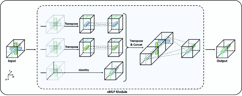
Figure 6: The sparse-MLP module proposed in sMLPNet [32]

References

- Cao et al. [2023] Guiping Cao, Shengda Luo, Wenjian Huang, Xiangyuan Lan, Dongmei Jiang, Yaowei Wang, and Jianguo Zhang. Strip-mlp: Efficient token interaction for vision mlp. In ICCV, pages 1494–1504, 2023.
- Chen et al. [2023] Shoufa Chen, Enze Xie, Chongjian Ge, Runjian Chen, Ding Liang, and Ping Luo. Cyclemlp: A mlp-like architecture for dense visual predictions. IEEE TPAMI, 2023.
- Chen et al. [2019] Weijie Chen, Di Xie, Yuan Zhang, and Shiliang Pu. All you need is a few shifts: Designing efficient convolutional neural networks for image classification. In CVPR, pages 7241–7250, 2019.
- Cheng et al. [2017] Gong Cheng, Junwei Han, and Xiaoqiang Lu. Remote sensing image scene classification: Benchmark and state of the art. Proceedings of the IEEE, 105(10):1865–1883, 2017.
- Cubuk et al. [2020] Ekin D Cubuk, Barret Zoph, Jonathon Shlens, and Quoc V Le. Randaugment: Practical automated data augmentation with a reduced search space. In CVPR, pages 702–703, 2020.
- Dai et al. [2017] Jifeng Dai, Haozhi Qi, Yuwen Xiong, Yi Li, Guodong Zhang, Han Hu, and Yichen Wei. Deformable convolutional networks. In ICCV, pages 764–773, 2017.
- Deng et al. [2009] Jia Deng, Wei Dong, Richard Socher, Li-Jia Li, Kai Li, and Li Fei-Fei. Imagenet: A large-scale hierarchical image database. In CVPR, pages 248–255, 2009.
- Dosovitskiy et al. [2021] Alexey Dosovitskiy, Lucas Beyer, Alexander Kolesnikov, Dirk Weissenborn, Xiaohua Zhai, Thomas Unterthiner, Mostafa Dehghani, Matthias Minderer, Georg Heigold, Sylvain Gelly, et al. An image is worth 16x16 words: Transformers for image recognition at scale. ICLR, 2021.
- Fukushima [1975] Kunihiko Fukushima. Cognitron: A self-organizing multilayered neural network. Biological cybernetics, 20(3-4):121–136, 1975.
- Fukushima [1980] Kunihiko Fukushima. Neocognitron: A self-organizing neural network model for a mechanism of pattern recognition unaffected by shift in position. Biological cybernetics, 36(4):193–202, 1980.
- Guo et al. [2022] Jianyuan Guo, Yehui Tang, Kai Han, Xinghao Chen, Han Wu, Chao Xu, Chang Xu, and Yunhe Wang. Hire-mlp: Vision mlp via hierarchical rearrangement. In CVPR, pages 826–836, 2022.
- Hassani et al. [2021] Ali Hassani, Steven Walton, Nikhil Shah, Abulikemu Abuduweili, Jiachen Li, and Humphrey Shi. Escaping the big data paradigm with compact transformers. arXiv preprint arXiv:2104.05704, 2021.
- He et al. [2016] Kaiming He, Xiangyu Zhang, Shaoqing Ren, and Jian Sun. Deep residual learning for image recognition. In CVPR, pages 770–778, 2016.
- He et al. [2022] Kaiming He, Xinlei Chen, Saining Xie, Yanghao Li, Piotr Dollár, and Ross Girshick. Masked autoencoders are scalable vision learners. In CVPR, pages 16000–16009, 2022.
- Hou et al. [2022] Qibin Hou, Zihang Jiang, Li Yuan, Ming-Ming Cheng, Shuicheng Yan, and Jiashi Feng. Vision permutator: A permutable mlp-like architecture for visual recognition. IEEE TPAMI, 45(1):1328–1334, 2022.
- Hubel and Wiesel [1962] David H Hubel and Torsten N Wiesel. Receptive fields, binocular interaction and functional architecture in the cat’s visual cortex. The Journal of physiology, 160(1):106, 1962.
- Hubel and Wiesel [1965] David H Hubel and Torsten N Wiesel. Receptive fields and functional architecture in two nonstriate visual areas (18 and 19) of the cat. Journal of neurophysiology, 28(2):229–289, 1965.
- Kermany et al. [2018] Daniel S Kermany, Michael Goldbaum, Wenjia Cai, Carolina CS Valentim, Huiying Liang, Sally L Baxter, Alex McKeown, Ge Yang, Xiaokang Wu, Fangbing Yan, et al. Identifying medical diagnoses and treatable diseases by image-based deep learning. cell, 172(5):1122–1131, 2018.
- Krizhevsky et al. [2009] Alex Krizhevsky, Geoffrey Hinton, et al. Learning multiple layers of features from tiny images. Citeseer, Tech. Rep., 2009.
- Krizhevsky et al. [2017] Alex Krizhevsky, Ilya Sutskever, and Geoffrey E Hinton. Imagenet classification with deep convolutional neural networks. Communications of the ACM, 60(6):84–90, 2017.
- LeCun et al. [1989a] Yann LeCun, Bernhard Boser, John S Denker, Donnie Henderson, Richard E Howard, Wayne Hubbard, and Lawrence D Jackel. Backpropagation applied to handwritten zip code recognition. Neural computation, 1(4):541–551, 1989a.
- LeCun et al. [1998] Yann LeCun, Léon Bottou, Yoshua Bengio, and Patrick Haffner. Gradient-based learning applied to document recognition. Proceedings of the IEEE, 86(11):2278–2324, 1998.
- LeCun et al. [1989b] Yann LeCun et al. Generalization and network design strategies. Connectionism in perspective, 19(143-155):18, 1989b.
- Li et al. [2023] Jiachen Li, Ali Hassani, Steven Walton, and Humphrey Shi. Convmlp: Hierarchical convolutional mlps for vision. In CVPR, pages 6306–6315, 2023.
- Lian et al. [2021] Dongze Lian, Zehao Yu, Xing Sun, and Shenghua Gao. As-mlp: An axial shifted mlp architecture for vision. arXiv preprint arXiv:2107.08391, 2021.
- Lin et al. [2019] Ji Lin, Chuang Gan, and Song Han. Tsm: Temporal shift module for efficient video understanding. In CVPR, pages 7083–7093, 2019.
- Liu et al. [2021a] Hanxiao Liu, Zihang Dai, David So, and Quoc V Le. Pay attention to mlps. NeurIPS, 34:9204–9215, 2021a.
- Liu et al. [2021b] Ze Liu, Yutong Lin, Yue Cao, Han Hu, Yixuan Wei, Zheng Zhang, Stephen Lin, and Baining Guo. Swin transformer: Hierarchical vision transformer using shifted windows. In ICCV, pages 10012–10022, 2021b.
- Loshchilov and Hutter [2019] Ilya Loshchilov and Frank Hutter. Decoupled weight decay regularization. ICLR, 2019.
- Radosavovic et al. [2020] Ilija Radosavovic, Raj Prateek Kosaraju, Ross Girshick, Kaiming He, and Piotr Dollár. Designing network design spaces. In CVPR, pages 10428–10436, 2020.
- Simonyan and Zisserman [2015] Karen Simonyan and Andrew Zisserman. Very deep convolutional networks for large-scale image recognition. ICLR, 2015.
- Tang et al. [2022a] Chuanxin Tang, Yucheng Zhao, Guangting Wang, Chong Luo, Wenxuan Xie, and Wenjun Zeng. Sparse mlp for image recognition: Is self-attention really necessary? In AAAI, pages 2344–2351, 2022a.
- Tang et al. [2022b] Yehui Tang, Kai Han, Jianyuan Guo, Chang Xu, Yanxi Li, Chao Xu, and Yunhe Wang. An image patch is a wave: Phase-aware vision mlp. In CVPR, pages 10935–10944, 2022b.
- Tolstikhin et al. [2021] Ilya O Tolstikhin, Neil Houlsby, Alexander Kolesnikov, Lucas Beyer, Xiaohua Zhai, Thomas Unterthiner, Jessica Yung, Andreas Steiner, Daniel Keysers, Jakob Uszkoreit, et al. Mlp-mixer: An all-mlp architecture for vision. NeurIPS, 34:24261–24272, 2021.
- Touvron et al. [2021] Hugo Touvron, Matthieu Cord, Matthijs Douze, Francisco Massa, Alexandre Sablayrolles, and Hervé Jégou. Training data-efficient image transformers & distillation through attention. In ICML, pages 10347–10357, 2021.
- Touvron et al. [2022] Hugo Touvron, Piotr Bojanowski, Mathilde Caron, Matthieu Cord, Alaaeldin El-Nouby, Edouard Grave, Gautier Izacard, Armand Joulin, Gabriel Synnaeve, Jakob Verbeek, et al. Resmlp: Feedforward networks for image classification with data-efficient training. IEEE TPAMI, 2022.
- Trockman and Kolter [2022] Asher Trockman and J Zico Kolter. Patches are all you need? arXiv preprint arXiv:2201.09792, 2022.
- Vaswani et al. [2017] Ashish Vaswani, Noam Shazeer, Niki Parmar, Jakob Uszkoreit, Llion Jones, Aidan N Gomez, Łukasz Kaiser, and Illia Polosukhin. Attention is all you need. NeurIPS, 30, 2017.
- Vinyals et al. [2016] Oriol Vinyals, Charles Blundell, Timothy Lillicrap, Daan Wierstra, et al. Matching networks for one shot learning. NeurIPS, 29, 2016.
- Wang et al. [2021] Wenhai Wang, Enze Xie, Xiang Li, Deng-Ping Fan, Kaitao Song, Ding Liang, Tong Lu, Ping Luo, and Ling Shao. Pyramid vision transformer: A versatile backbone for dense prediction without convolutions. In ICCV, pages 568–578, 2021.
- Wang et al. [2022] Ziyu Wang, Wenhao Jiang, Yiming M Zhu, Li Yuan, Yibing Song, and Wei Liu. Dynamixer: a vision mlp architecture with dynamic mixing. In ICML, pages 22691–22701, 2022.
- Wightman et al. [2021] Ross Wightman, Hugo Touvron, and Hervé Jégou. Resnet strikes back: An improved training procedure in timm. arXiv preprint arXiv:2110.00476, 2021.
- Wu et al. [2021] Haiping Wu, Bin Xiao, Noel Codella, Mengchen Liu, Xiyang Dai, Lu Yuan, and Lei Zhang. Cvt: Introducing convolutions to vision transformers. In ICCV, pages 22–31, 2021.
- Xiao et al. [2017] Han Xiao, Kashif Rasul, and Roland Vollgraf. Fashion-mnist: a novel image dataset for benchmarking machine learning algorithms. arXiv preprint arXiv:1708.07747, 2017.
- Xie et al. [2017] Saining Xie, Ross Girshick, Piotr Dollár, Zhuowen Tu, and Kaiming He. Aggregated residual transformations for deep neural networks. In CVPR, pages 1492–1500, 2017.
- Yu et al. [2021] Tan Yu, Xu Li, Yunfeng Cai, Mingming Sun, and Ping Li. S2-mlpv2: Improved spatial-shift mlp architecture for vision. arXiv preprint arXiv:2108.01072, 2021.
- Yu et al. [2022] Tan Yu, Xu Li, Yunfeng Cai, Mingming Sun, and Ping Li. S2-mlp: Spatial-shift mlp architecture for vision. In Winter Conference on Applications of Computer Vision, pages 297–306, 2022.
- Yun et al. [2019] Sangdoo Yun, Dongyoon Han, Seong Joon Oh, Sanghyuk Chun, Junsuk Choe, and Youngjoon Yoo. Cutmix: Regularization strategy to train strong classifiers with localizable features. In ICCV, pages 6023–6032, 2019.
- Zhang et al. [2017] Hongyi Zhang, Moustapha Cisse, Yann N Dauphin, and David Lopez-Paz. mixup: Beyond empirical risk minimization. arXiv preprint arXiv:1710.09412, 2017.
- Zhang et al. [2022] Zizhao Zhang, Han Zhang, Long Zhao, Ting Chen, Sercan Ö Arik, and Tomas Pfister. Nested hierarchical transformer: Towards accurate, data-efficient and interpretable visual understanding. In AAAI, pages 3417–3425, 2022.
- Zhong et al. [2020] Zhun Zhong, Liang Zheng, Guoliang Kang, Shaozi Li, and Yi Yang. Random erasing data augmentation. In AAAI, pages 13001–13008, 2020.