DP-SGD Without Clipping:
The Lipschitz Neural Network Way

Abstract

State-of-the-art approaches for training Differentially Private (DP) Deep Neural Networks (DNN) faces difficulties to estimate tight bounds on the sensitivity of the network’s layers, and instead rely on a process of per-sample gradient clipping. This clipping process not only biases the direction of gradients but also proves costly both in memory consumption and in computation. To provide sensitivity bounds and bypass the drawbacks of the clipping process, our theoretical analysis of Lipschitz constrained networks reveals an unexplored link between the Lipschitz constant with respect to their input and the one with respect to their parameters. By bounding the Lipschitz constant of each layer with respect to its parameters we guarantee DP training of these networks. This analysis not only allows the computation of the aforementioned sensitivities at scale but also provides leads on to how maximize the gradient-to-noise ratio for fixed privacy guarantees. To facilitate the application of Lipschitz networks and foster robust and certifiable learning under privacy guarantees, we provide a Python package that implements building blocks allowing the construction and private training of such networks.

1 Introduction

Machine learning relies more than ever on foundational models, and such practices raise questions about privacy. Differential privacy allows to develop methods for training models that preserve the privacy of individual data points in the training set. The field seeks to enable deep learning on sensitive data, while ensuring that models do not inadvertently memorize or reveal specific details about individual samples in their weights. This involves incorporating privacy-preserving mechanisms into the design of deep learning architectures and training algorithms, whose most popular example is Differentially Private Stochastic Gradient Descent (DP-SGD) [1]. One main drawback of classical DP-SGD methods is that they require costly per-sample backward processing and gradient clipping. In this paper, we offer a new method that unlocks fast differentially private training through the use of Lipschitz constrained neural networks. Additionally, this method offers new opportunities for practitioners that wish to easily "DP-fy" [2] the training procedure of a deep neural network.

Differential privacy fundamentals. Informally, differential privacy is a definition that quantifies how much the change of a single sample in a dataset affects the range of a stochastic function (here the DP training), called mechanism in this context. This quantity can be bounded in an inequality involving two parameters $\epsilon$ and $\delta$. A mechanism fulfilling such inequality is said $(\epsilon,\delta)$-DP (see Definition 1). This definition is universally accepted as a strong guarantee against privacy leakages under various scenarii, including data aggregation or post-processing [3]. A popular rule of thumb suggests using $\epsilon\leq 10$ and $\delta<\frac{1}{N}$ with $N$ the number of records [2] for mild guarantees. In practice, most classic algorithmic procedures (called queries in this context) do not readily fulfill the definition for useful values of $(\epsilon,\delta)$, in particular the deterministic ones: randomization is mandatory. This randomization comes at the expense of “utility”, i.e the usefulness of the output for downstream tasks [4]. The goal is then to strike a balance between privacy and utility, ensuring that the released information remains useful and informative for the intended purpose while minimizing the risk of privacy breaches. The privacy/utility trade-off yields a Pareto front, materialized by plotting $\epsilon$ against a measurement of utility, such as validation accuracy for a classification task.

Private gradient descent. The SGD algorithm consists of a sequence of queries that (i) take the dataset in input, sample a minibatch from it, and return the gradient of the loss evaluated on the minibatch, before (ii) performing a descent step following the gradient direction. The sensitivity (see Definition 2) of SGD queries is proportional to the norm of the per-sample gradients. DP-SGD turns each query into a Gaussian mechanism by perturbing the gradients with a noise $\zeta$. The upper bound on gradient norms is generally unknown in advance, which leads practitioners to clip it to $C>0$, in order to bound the sensitivity manually. This is problematic for several reasons: 1. Hyper-parameter search on the broad-range clipping value $C$ is required to train models with good privacy/utility trade-offs [5], 2. The computation of per-sample gradients is expensive: DP-SGD is usually slower and consumes more memory than vanilla SGD, in particular for the large batch sizes often used in private training [6], 3. Clipping the per-sample gradients biases their average [7]. This is problematic as the average direction is mainly driven by misclassified examples, that carry the most useful information for future progress.

⬇

model = DP_Sequential( # step 1: use DP_Sequential to build a model

[

# step 2: add Lipschitz layers of known sensitivity

DP_BoundedInput(input_shape=(28, 28, 1), upper_bound=20.),

DP_SpectralConv2D(filters=16, kernel_size=3, use_bias=False),

DP_GroupSort(2),

DP_Flatten(),

DP_SpectralDense(10),

],

noise_multiplier = 1.2, # step 3: choose DP parameters

sampling_probability = batch_size / dataset_size,

) # step 4: compile the model, and choose any first order optimizer

model.compile(loss=DP_Crossentropy(), optimizer=Adam(1e-3))

model.fit( # step 5: train the model and measure the DP guarantees

train_dataset, validation_data=val_dataset,

epochs=num_epochs, callbacks=[DP_Accountant()]

)

Figure 1: An example of usage of our framework, illustrating how to create a small Lipschitz VGG and how to train it under $(\epsilon,\delta)$-DP guarantees while reporting $(\epsilon,\delta)$ values.

An unexplored approach: Lipschitz constrained networks. We propose to train neural networks for which the parameter-wise gradients are provably and analytically bounded during the whole training procedure, in order to get rid of the clipping process. This allows for rapid training of models without a need for tedious hyper-parameter optimization.

The main reason why this approach has not been experimented much in the past is that upper bounding the gradient of neural networks is often intractable. However, by leveraging the literature of Lipschitz constrained networks [8], we show that these networks allows to estimate their gradient bound. This yields tight bounds on the sensitivity of SGD steps, making their transformation into Gaussian mechanisms inexpensive - hence the name Clipless DP-SGD.

Informally, the Lipschitz constant quantifies the rate at which the function’s output varies with respect to changes in its input. A Lipschitz constrained network is one in which its weights and activations are constrained such that it can only represent $l$-Lipschitz functions. In this work, we will focus our attention on feed-forward networks (refer to Definition 3). Note that the most common architectures, such as Convolutional Neural Networks (CNNs), Fully Connected Networks (FCNs), Residual Networks (ResNets), or patch-based classifiers (like MLP-Mixers), all fall under the category of feed-forward networks. We will also tackle the particular case of Gradient Norm Preserving (GNP) networks, a subset of Lipschitz networks that enjoy tighter bounds (see appendix).

Contributions

While the properties of Lipschitz constrained networks regarding their inputs are well explored, the properties with respect to its parameters remain non-trivial. This work provides a first step to fill this gap: our analysis shows that under appropriate architectural constraints, a $l$-Lipschitz network has a tractable, finite Lipschitz constant with respect to its parameters. We prove that this Lipschitz constant allows for easy estimation of the sensitivity of the gradient computation queries. The prerequisite and details of the method to compute the sensitivities are explained in Section 2.

Our contributions are the following:

1. We extend the field of applications of Lipschitz constrained neural networks. So far the literature focused on Lipschitzness with respect to the inputs: we extend the framework to compute the Lipschitzness with respect to the parameters. This is exposed in Section 2.

2. We propose a general framework to handle layer gradient steps as Gaussian mechanisms that depends on the loss and the model structure. Our framework covers widely used architectures, including VGG and ResNets.

3. We show that SGD training of deep neural networks can be achieved without gradient clipping using Lipschitz layers. This allows the use of larger networks and larger batch sizes, as illustrated by our experiments in Section 4.

4. We establish connections between Gradient Norm Preserving (GNP) networks and improved privacy/utility trade-offs (Section 3.1).

5. Finally, a Python package companions the project, with pre-computed Lipschitz constant and noise for each layer type, ready to be forked on any problem of interest (Section 3.2).

1.1 Differential Privacy and Lipschitz Networks

The definition of DP relies on the notion of neighboring datasets, i.e datasets that vary by at most one example. We highlight below the central tools related to the field, inspired from [9].

Definition 1 ($(\epsilon,\delta)$-Differential Privacy).

A labeled dataset $\mathcal{D}$ is a finite collection of input/label pairs $\mathcal{D}=\{(x_{1},y_{1}),(x_{2},y_{2}),\ldots...(x_{N},y_{N})\}$. Two datasets $\mathcal{D}$ and $\mathcal{D}^{\prime}$ are said to be neighboring for the “replace-one” relation if they differ by at most one sample: $\mathcal{D}^{\prime}=\mathcal{D}\cup\{(x_{i}^{\prime},y_{i}^{\prime})\}\setminus\{(x_{i},y_{i})\}$.
Let $\epsilon$ and $\delta$ be two non-negative scalars. A mechanism $\mathcal{A}$ is $(\epsilon,\delta)$-DP if for any two neighboring datasets $\mathcal{D}$ and $\mathcal{D}^{\prime}$, and for any $S\subseteq\text{range}(\mathcal{A})$:

$$\mathbb{P}[\mathcal{A}(\mathcal{D})\in S]\leq e^{\epsilon}\times\mathbb{P}[\mathcal{A}(\mathcal{D}^{\prime})\in S]+\delta.$$ (1)

A cookbook to create a $(\epsilon,\delta)$-DP mechanism from a query is to compute its sensitivity $\Delta$ (see Definition 2), and to perturb its output by adding a Gaussian noise of predefined variance $\zeta^{2}=\Delta^{2}\sigma^{2}$, where the $(\epsilon,\delta)$-DP guarantees depends on $\sigma$. This yields what is called a Gaussian mechanism [3].

Definition 2 ($l_{2}$-sensitivity).

Let $\mathcal{M}$ be a query mapping from the space of the datasets to $\mathbb{R}^{p}$. Let $\mathcal{N}$ be the set of all possible pairs of neighboring datasets $\mathcal{D},\mathcal{D}^{\prime}$. The $l_{2}$ sensitivity of $\mathcal{M}$ is defined by:

$$\Delta(\mathcal{M})=\underset{\mathcal{D},\mathcal{D}^{\prime}\in\mathcal{N}}{\max}\|\mathcal{M}(D)-\mathcal{M}(D^{\prime})\|_{2}.$$ (2)

Differentially Private SGD. The classical algorithm keeps track of $(\epsilon,\delta)$-DP values with a moments accountant [1] which allows to keep track of privacy guarantees at each epoch, by composing different sub-mechanisms. For a dataset with $N$ records and a batch size $b$, it relies on two parameters: the sampling ratio ${p=\frac{b}{N}}$ and the “noise multiplier” $\sigma$ defined as the ratio between effective noise strength $\zeta$ and sensitivity $\Delta$. Bounds on gradient norm can be turned into bounds on sensitivity of SGD queries. In “replace-one” policy for $(\epsilon,\delta)$-DP accounting, if the gradients are bounded by $K>0$, the sensitivity of the gradients averaged on a minibatch of size $b$ is $\Delta=2K/b$..

Crucially, the algorithm requires a bound on $\|\nabla_{\theta}\mathcal{L}(\hat{y},y)\|_{2}\leq K$. The whole difficulty lies in bounding tightly this value in advance for neural networks. Currently, gradient clipping serves as a patch to circumvent the issue [1]. Unfortunately, clipping individual gradients in the batch is costly and will bias the direction of their average, which may induce underfitting [7].

Lipschitz constrained networks. Our proposed solution comes from the observation that the norm of the gradient and the Lipschitz constant are two sides of the same coin. The function $f:\mathbb{R}^{m}\rightarrow\mathbb{R}^{n}$ is said $l$-Lipschitz for $l_{2}$ norm if for every $x,y\in\mathbb{R}^{m}$ we have $\|f(x)-f(y)\|_{2}\leq l\|x-y\|_{2}$. Per Rademacher’s theorem [10], its gradient is bounded: $\|\nabla_{x}f\|\leq l$. Reciprocally, continuous functions gradient bounded by $l$ are $l$-Lipschitz.

In Lipschitz networks, the literature has predominantly concentrated on investigating the control of Lipschitzness with respect to the inputs (i.e bounding $\nabla_{x}f$), primarily motivated by concerns of robustness [11]. However, in this work, we will demonstrate that it is also possible to control Lipschitzness with respect to parameters (i.e bounding $\nabla_{\theta}f$), which is essential for ensuring privacy. Our first contribution will point out the tight link that exists between those two quantities.

Definition 3 (Lipschitz feed-forward neural network).

A feedforward neural network of depth $D$, with input space $\mathcal{X}\subset\mathbb{R}^{n}$, output space $\mathcal{Y}\subset\mathbb{R}^{K}$ (e.g logits), and parameter space $\Theta\subset\mathbb{R}^{p}$, is a parameterized function $f:\Theta\times\mathcal{X}\rightarrow\mathcal{Y}$ defined by the sequential composition of layers $f_{d}$:

$$f(\theta,x)\vcentcolon=\left(f_{D}(\theta_{d})\circ\ldots\circ f_{2}(\theta_{2})\circ f_{1}(\theta_{1})\right)(x).$$ (3)

The parameters of the layers are denoted by $\theta=(\theta_{d})_{1\leq d\leq D}\in\Theta$. For affine layers, it corresponds to bias and weight matrix $\theta_{d}=(W_{d},b_{d})$. For activation functions, there is no parameters: $\theta_{d}=\varnothing$.

Lipschitz networks are feed-forward networks, with the additionnal constraint that each layer ${x_{d}\mapsto f_{d}(\theta_{d},x_{d})\vcentcolon=y_{d}}$ is $l_{d}$-Lipschitz for all $\theta_{d}$. Consequently, the function ${x\mapsto f(\theta,x)}$ is $l$-Lipschitz with ${l=l_{1}\times\ldots\times l_{d}}$ for all $\theta\in\Theta$.

In practice, this is enforced by using activations with Lipschitz constant $l_{d}$, and by applying a constraint $\Pi:\mathbb{R}^{p}\rightarrow\Theta$ on the weights of affine layers. This corresponds to spectrally normalized matrices [12, 13], since for affine layers we have ${l_{d}=\|W_{d}\|_{2}\vcentcolon=\underset{\|x\|\leq 1}{\max}\|W_{d}x\|_{2}}$ hence $\Theta=\{\|W_{d}\|\leq l_{q}\}$. The seminal work of [8] proved that universal approximation in the set of $l$-Lipschitz functions was achievable by this family of architectures. Concurrent approaches are based on regularization (like in [14, 15, 16]) but they fail to produce formal guarantees. While they have primarily been studied in the context of adversarial robustness [11, 17], recent works have revealed additional properties of these networks, such as improved generalization [13, 18]. However, the properties of their parameter gradient $\nabla_{\theta}f(\theta,x)$ remain largely unexplored.

2 Clipless DP-SGD with $l$-Lipschitz networks

Our framework consists of 1. a method that computes the maximum gradient norm of a network with respect to its parameters to obtain a per-layer sensitivity $\Delta_{d}$, 2. a moments accountant that relies on the per-layer sensitivities to compute $(\epsilon,\delta)$-DP guarantees. The method 1. is based on the recursive formulation of the chain rule involved in backpropagation, while 2. keeps track of $(\epsilon,\delta)$-DP values with RDP accounting. It requires some natural assumptions that we highlight below.

Requirement 1 (Lipschitz loss.).

The loss function $\hat{y}\mapsto\mathcal{L}(\hat{y},y)$ must be $L$-Lipschitz with respect to the logits $\hat{y}$ for all ground truths $y\in\mathcal{Y}$. This is notably the case of Categorical Softmax-Crossentropy.

The Lipschitz constants of common classification losses can be found in the appendix.

Requirement 2 (Bounded input).

There exists $X_{0}>0$ such that for all $x\in\mathcal{X}$ we have $\|x\|\leq X_{0}$.

While there exist numerous approaches for the parametrization of Lipschitz networks (e.g differentiable re-parametrization [19, 8], optimization over matrix manifolds [20] or projections [21]), our framework only provides sensitivity bounds for projection-based algorithms (see appendix).

Requirement 3 (Lipschitz projection).

The Lipschitz constraints must be enforced with a projection operator $\Pi:\mathbb{R}^{p}\rightarrow\Theta$. This corresponds to Tensorflow [22] constraints and Pytorch [23] hooks. Projection is a post-processing of private gradients: it induces no privacy leakage [3].

To compute the per-layer sensitivities, our framework mimics the backpropagation algorithm, where Vector-Jacobian products (VJP) are replaced by Scalar-Scalar products of element-wise bounds. For an arbitrary layer $x_{d}\mapsto f_{d}(\theta_{d},x_{d})\vcentcolon=y_{d}$ the operation is sketched below:

$$\underbrace{\nabla_{x_{d}}\mathcal{L}\vcentcolon=(\nabla_{y_{d}}\mathcal{L})\frac{\partial f_{d}}{\partial x_{d}}}_{\text{Vector-Jacobian product: backpropagate gradients}}\implies\underbrace{\|\nabla_{x_{d}}\mathcal{L}\|_{2}\leq\|\nabla_{y_{d}}\mathcal{L}\|_{2}\times{\color[rgb]{0.28515625,0.765625,0.62109375}\left\|\frac{\partial f_{d}}{\partial x_{d}}\right\|_{2}}.}_{\text{Scalar-Scalar product: backpropagate bounds}}$$ (4)

The notation $\|\cdot\|_{2}$ must be understood as the spectral norm for Jacobian matrices, and the Euclidean norm for gradient vectors. The scalar-scalar product is inexpensive. For Lipschitz layers the spectral norm of the Jacobian $\|\frac{\partial f}{\partial x}\|$ is kept constant during training with projection operator $\Pi$. The bound of the gradient with respect to the parameters then takes a simple form:

$$\|\nabla_{\theta_{d}}\mathcal{L}\|_{2}=\|\nabla_{y_{d}}\mathcal{L}\|_{2}\times{\color[rgb]{0.921875,0.70703125,0.140625}\left\|\frac{\partial f_{d}}{\partial\theta_{d}}\right\|_{2}}.$$ (5)

Once again the operation is inexpensive. The upper bound $\left\|\frac{\partial f}{\partial\theta}\right\|_{2}$ typically depends on the supremum of $\|x_{d}\|_{2}$, that can also be analytically bounded, as exposed in the following section.

2.1 Backpropagation for bounds

The pseudo-code of Clipless DP-SGD is sketched in Algorithm 2. The algorithm avoids clipping by computing a per-layer bound on the element-wise gradient norm. The computation of this per-layer bound is described by Algorithm 1 (graphically explained in Figure 2). Crucially, it requires to compute the spectral norm of the Jacobian of each layer with respect to input and parameters.

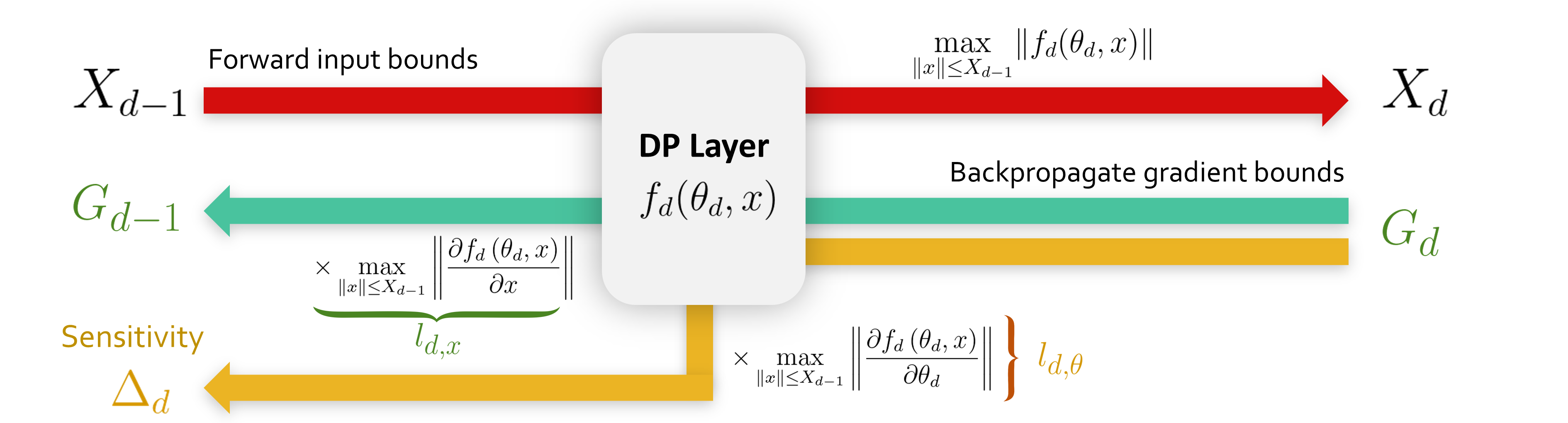
Figure 2: Backpropagation for bounds, Algorithm 1. Compute the per-layer sensitivity $\Delta_{d}$.

Input bound propagation (line  2). We compute $X_{d}={\color[rgb]{0.83203125,0.0546875,0.05078125}\max_{\|x\|\leq X_{d-1}}\|f_{d}(x)\|_{2}}$. For activation functions it depends on their range. For linear layers, it depends on the spectral norm of the operator itself. This quantity can be computed with SVD or Power Iteration [24, 19], and constrained during training using projection operator $\Pi$. In particular, it covers the case of convolutions, for which tight bounds are known [25]. For affine layers, it additionally depends on the amplitude of the bias $\|b_{d}\|$.

Remark 1 (Tighter bounds in literature.).

Although libraries such as Decomon [26] or auto-LiRPA [27] provide tighter bounds for $X_{d}$ via linear relaxations [28, 29], our approach is capable of delivering practically tighter bounds than worst-case scenarios thanks to the projection operator $\Pi$, while also being significantly less computationally expensive. Moreover, hybridizing our method with scalable certification methods can be a path for future extensions.

Computing maximum gradient norm (line 6). We bound the Jacobian $\frac{\partial f_{d}(\theta_{d},x)}{\partial\theta_{d}}$. In neural networks, the parameterized layers $f(\theta,x)$ (fully connected, convolutions) are bilinear operators. Hence we typically obtain bounds of the form:

$${\color[rgb]{0.921875,0.70703125,0.140625}\left\|\frac{\partial f_{d}(\theta_{d},x)}{\partial\theta_{d}}\right\|_{2}}\leq K(f_{d},\theta_{d})\|x\|_{2}\leq K(f_{d},\theta_{d}){\color[rgb]{0.83203125,0.0546875,0.05078125}X_{d-1}},$$ (6)

where $K(f_{d},\Theta_{d})$ is a constant that depends on the nature of the operator. $X_{d-1}$ is obtained in line 2 with input bound propagation. Values of $K(f_{d},\theta_{d})$ for popular layers are pre-computed in the library.

Backpropagate cotangeant vector bounds (line 7).

We bound the Jacobian ${\color[rgb]{0.28515625,0.765625,0.62109375}\frac{\partial f_{d}(\theta_{d},x)}{\partial x}}$. For activation functions this value can be hard-coded, while for affine layers it is the spectral norm of the linear operator. Like before, this value is constrained with projection operator $\Pi$.

Algorithm 1 Backpropagation for Bounds$(f,X)$

Input: Feed-forward architecture $f(\theta,\cdot)=f_{D}(\theta_{D},\cdot)\circ\ldots\circ f_{1}(\theta_{1},\cdot)$
Input: Weights $\theta=(\theta_{1},\theta_{2},\ldots\theta_{D})$, input bound $X_{0}$

1:for all layers $1\leq d\leq D$ do

2:     $X_{d}\leftarrow{\color[rgb]{0.83203125,0.0546875,0.05078125}\underset{\|x\|\leq X_{d-1}}{\max}\|f_{d}(\theta_{d},x)\|_{2}}.$ $\triangleright$ Input bounds propagation

3:end for

4:$G\leftarrow L/b.$$\triangleright$ Lipschitz constant of the loss for batchsize b

5:for all layers $D\geq d\geq 1$ do

6:     $\Delta_{d}\leftarrow G{\color[rgb]{0.921875,0.70703125,0.140625}\underset{\|x\|\leq X_{d-1}}{\max}\|\frac{\partial f_{d}(\theta_{d},x)}{\partial\theta_{d}}\|_{2}}$. $\triangleright$ Compute sensitivity from gradient norm

7:     $G\leftarrow G{\color[rgb]{0.28515625,0.765625,0.62109375}\underset{\|x\|\leq X_{d-1}}{\max}\|\frac{\partial f_{d}(\theta_{d},x)}{\partial x}\|_{2}}=G{\color[rgb]{0.28515625,0.765625,0.62109375}l_{d}}$. $\triangleright$ Backpropagate cotangeant vector bounds

8:end for

9:return sensitivities $\Delta_{1},\Delta_{2}\ldots,\Delta_{D}$

Algorithm 2 Clipless DP-SGD with local sensitivity accounting

Input: Feed-forward architecture $f(\theta,\cdot)=f_{D}(\theta_{D},\cdot)\circ\ldots\circ f_{1}(\theta_{1},\cdot)$
Input: Initial weights $\theta=(\theta_{1},\theta_{1},\ldots\theta_{D})$, learning rate $\eta$, noise multiplier $\sigma$.

1:repeat

2:     $\Delta_{1},\Delta_{2}\ldots\Delta_{D}\leftarrow$ Backpropagation for Bounds$(f,X)$.

3:     Update Moment Accountant state with local sensitivities $\Delta_{1},\Delta_{2},\ldots\Delta_{d}$.

4:     Sample a batch $\mathcal{B}=\{(x_{1},y_{1}),(x_{2},y_{2}),\ldots,(x_{b},y_{b})\}$.

5:     Compute per-layer averaged gradient: $g_{d}\vcentcolon=\frac{1}{b}\sum_{i=1}^{b}\nabla_{\theta_{d}}\mathcal{L}(f(\theta,x_{i}),y_{i})).$

6:     Sample local noise: $\zeta_{d}\sim\mathcal{N}(0,\sigma\Delta_{d})$.

7:     Perform noisified gradient step: $\theta_{d}\leftarrow\theta_{d}-\eta(g_{d}+\zeta_{d})$.

8:     Enforce Lipschitz constraint with projection: $\theta_{d}\leftarrow\Pi(\theta_{d})$.

9:until privacy budget $(\epsilon,\delta)$-DP budget has been reached.

2.2 Privacy accounting for Clipless DP-SGD

Two strategies are available to keep track of $(\epsilon,\delta)$ values as the training progresses, based on accounting either a per-layer “local” sensitivity, either by aggregating them into a “global” sensitivity.

The “global” strategy. Illustrated in the appendix,this strategy simply aggregates the individual sensitivities $\Delta_{d}$ of each layer to obtain the global sensitivity of the whole gradient vector $\Delta=\sqrt{\sum_{d}\Delta_{d}^{2}}$. The origin of the clipping-based version of this strategy can be traced back to [30]. With noise variance $\sigma^{2}\Delta^{2}$ we recover the accountant that comes with DP-SGD. It tends to overestimate the true sensitivity (in particular for deep networks), but its implementation is straightforward with existing tools.

The “local” strategy. Recall that we are able to characterize the sensitivity $\Delta_{d}$ of every layer of the network. Hence, we can apply a different noise to each of the gradients. We dissect the whole training procedure in Figure 3. At same noise multiplier $\sigma$, it tends to produce a higher value of $\epsilon$ per epoch than “global” strategy, but has the advantage over the latter to add smaller effective noise $\zeta$ to each weight.

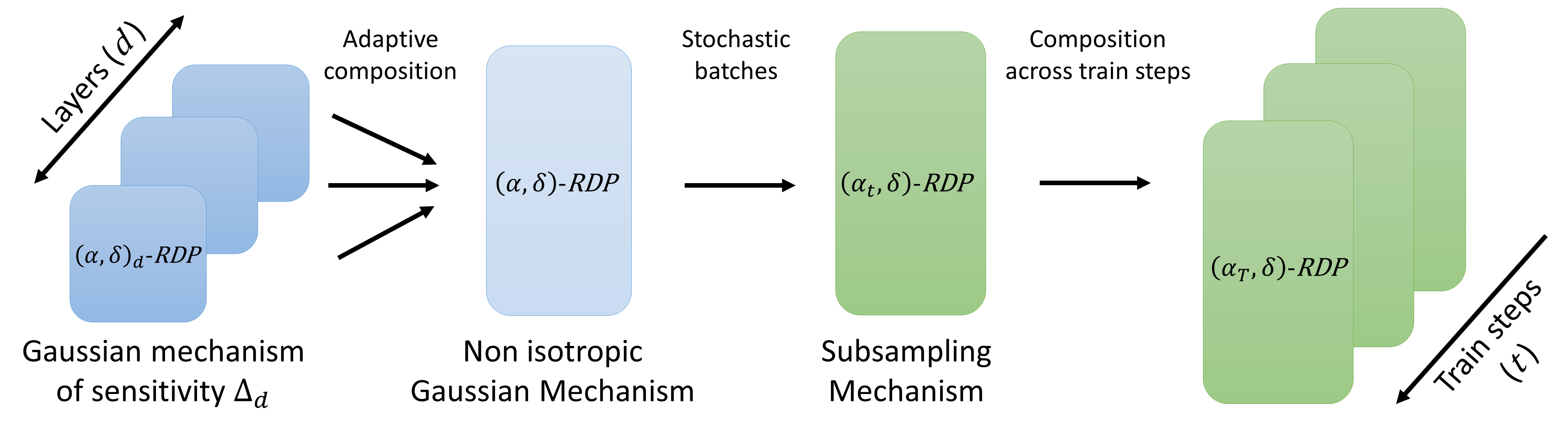
Figure 3: Accountant for locally enforced differential privacy. (i) The gradient query for each layer is turned into a Gaussian mechanism [9], (ii) their composition at the scale of the whole network is a non isotropic Gaussian mechanism, (iii) that benefits from amplification via sub-sampling [31], (iv) the train steps are composed over the course of training.

We rely on the autodp library [32, 33, 34] as it uses the Renyi Differential Privacy (RDP) adaptive composition theorem [35, 36], that ensures tighter bounds than naive DP composition.

3 From theory to practice

Beyond the application of Algorithms 1 and 2, our framework provides numerous opportunities to enhance our understanding of prevalent techniques identified in the literature. An in-depth exploration of these is beyond the scope of this work, so we focus on giving insights on promising tracks based on our theoretical analysis. In particular, we discuss how the tightness of the bound provided by Algorithm 1 can be influenced by working on the architecture, the input pre-processing and the loss post-processing.

3.1 Gradient Norm Preserving networks

We can manually derive the bounds obtained from Algorithm 2 across diverse configurations. Below, we conduct a sensitivity analysis on $l$-Lipschitz networks.

Theorem (informal) 1.

Gradient Norm of Lipschitz Networks. Assume that every layer $f_{d}$ is $K$-Lipschitz, i.e $l_{1}=\dots=l_{D}=K$. Assume that every bias is bounded by $B$. We further assume that each activation is centered in zero (e.g ReLU, tanh, GroupSort). We recall that $\theta=[\theta_{1},\theta_{2},\ldots\theta_{D}]$. Then the global upper bound of Algorithm 2 can be expanded analytically.

1. If $K<1$ we have: $\|\nabla_{\theta}\mathcal{L}(f(\theta,x),y)\|_{2}=\mathcal{O}\left(L\left(K^{D}(X_{0}+B)+1\right)\right).$
Due to the $K^{D}\ll 1$ term this corresponds to a vanishing gradient phenomenon [37]. The output of the network is essentially independent of its input, and the training is nearly impossible.

2. If $K>1$ we have: $\|\nabla_{\theta}\mathcal{L}(f(\theta,x),y)\|_{2}=\mathcal{O}\left(LK^{D}\left(X_{0}+B+1\right)\right).$
Due to the $K^{D}\gg 1$ term this corresponds to an exploding gradient phenomenon [38]. The upper bound becomes vacuous for deep networks: the added noise $\zeta$ is at risk of being too high.

3. If $K=1$ we have: $\|\nabla_{\theta}\mathcal{L}(f(\theta,x),y)\|_{2}=\mathcal{O}\left(L\left(\sqrt{D}+X_{0}\sqrt{D}+\sqrt{BX_{0}}D+BD^{3/2}\right)\right),$
which for linear layers without biases further simplify to $\mathcal{O}(L\sqrt{D}(1+X_{0}))$.

The formal statement can be found in appendix. From Theorem 1 we see that most favorable bounds are achieved by 1-Lipschitz neural networks with 1-Lipschitz layers. In classification tasks, they are not less expressive than conventional networks [18]. Hence, this choice of architecture is not at the expense of utility. Moreover an accuracy/robustness trade-off exists, determined by the choice of loss function [18]. However, setting $K=1$ merely ensures that $\|\nabla_{x}f\|\leq 1$, and in the worst-case scenario we have $\|\nabla_{x}f\|<1$ almost everywhere. This could result in a situation where the bound of case 3 in Theorem 1 is not tight, leading to an underfitting regime as in case $K<1$. With Gradient Norm Preserving (GNP) networks [17], we expect to mitigate this issue.

Controlling $K$ with Gradient Norm Preserving (GNP) networks.

GNP networks are 1-Lipschitz neural networks with the additional constraint that the Jacobian of layers consists of orthogonal matrices. They fulfill the Eikonal equation $\left\|\frac{\partial f_{d}(\theta_{d},x_{d})}{\partial x_{d}}\right\|_{2}=1$ for any intermediate activation $f_{d}(\theta_{d},x_{d})$. Without biases these networks are also norm preserving: $\|f(\theta,x)\|=\|x\|.$

As a consequence, the gradient of the loss with respect to the parameters is easily bounded by

$$\|\nabla_{\theta_{d}}\mathcal{L}\|={\color[rgb]{0.28515625,0.765625,0.62109375}\|\nabla_{y_{D}}\mathcal{L}\|}\times\left\|\frac{\partial f_{d}(\theta_{d},x_{d})}{\partial\theta_{d}}\right\|,$$ (7)

which for weight matrices $W_{d}$ further simplifies to $\|\nabla_{W_{d}}\mathcal{L}\|\leq{\color[rgb]{0.28515625,0.765625,0.62109375}\|\nabla_{y_{D}}\mathcal{L}\|}\times{\color[rgb]{0.83203125,0.0546875,0.05078125}\left\|f_{d-1}(\theta_{d-1},x_{d-1})\right\|}$. We see that this upper bound crucially depends on two terms than can be analyzed separately. On one hand, ${\color[rgb]{0.83203125,0.0546875,0.05078125}\left\|f_{d-1}(\theta_{d-1},x_{d-1})\right\|}$ depends on the scale of the input. On the other, ${\color[rgb]{0.28515625,0.765625,0.62109375}\|\nabla_{y_{D}}\mathcal{L}\|}$ depends on the loss, the predictions and the training stage. We show below how to intervene on these two quantities.

Remark 2 (Implementation of GNP Networks).

In practice, GNP are parametrized with GroupSort activation [8, 39], Householder activation [40], and orthogonal weight matrices [17, 41]. Strict orthogonality is challenging to enforce, especially for convolutions for which it is still an active research area (see [42, 43, 44, 45, 46] and references therein). Our line of work traces an additional motivation for the development of GNP and the bounds will strengthen as the field progresses.

Controlling ${\color[rgb]{0.83203125,0.0546875,0.05078125}X_{0}}$ with input pre-processing. The weight gradient norm $\|\nabla_{\theta_{d}}\mathcal{L}\|$ indirectly depends on the norm of the inputs. This observation implies that the pre-processing of input data significantly influences the bounding of sensitivity. Multiple strategies are available to keep the input’s norm under control: projection onto the ball (“norm clipping”), or projection onto the sphere (“normalization”). In the domain of natural images for instance, this result sheds light on the importance of color space such as RGB, HSV, YIQ, YUV or Grayscale. These strategies are natively handled by our library.

Controlling ${\color[rgb]{0.28515625,0.765625,0.62109375}L}$ with the hybrid approach, loss gradient clipping. As training progresses, the magnitude of ${\color[rgb]{0.28515625,0.765625,0.62109375}\|\nabla_{f}\mathcal{L}\|}$ tends to diminish when approaching a local minima, quickly falling below the upper bound and diminishing the gradient norm to noise ratio. To circumvent the issue, the gradient clipping strategy is still available in our framework. Crucially, instead of clipping the parameter gradient $\nabla_{\theta}\mathcal{L}$, any intermediate gradient $\nabla_{f_{d}}\mathcal{L}$ can be clipped during backpropagation. This can be achieved with a special “clipping layer” that behaves like the identity function at the forward pass, and clips the gradient during the backward pass. The resulting cotangeant vector is not a true gradient anymore, but rather a descent direction [47]. In vanilla DP-SGD the clipping is applied on the batched gradient $\nabla_{W_{d}}\mathcal{L}$ of size $b\times h^{2}$ for matrix weight ${W_{d}\in\mathbb{R}^{h\times h}}$ and clipping this vector can cause memory issues or slowdowns [6]. In our case, $\nabla_{y_{D}}\mathcal{L}$ is of size $b\times h$ which reduces overhead.

3.2 Lip-dp library

To foster and spread accessibility, we provide an opensource tensorflow library for Clipless DP-SGD training, named lip-dp. It provides an exposed Keras API for seamless usability. It is implemented as a wrapper over the Lipschitz layers of deel-lip library [48]. Its usage is illustrated in Figure 1.

4 Experimental results

We validate our implementation with a speed benchmark against competing approaches, and we present the privacy/utility Pareto front that can be obtained with GNP networks.

Speed and memory consumption.

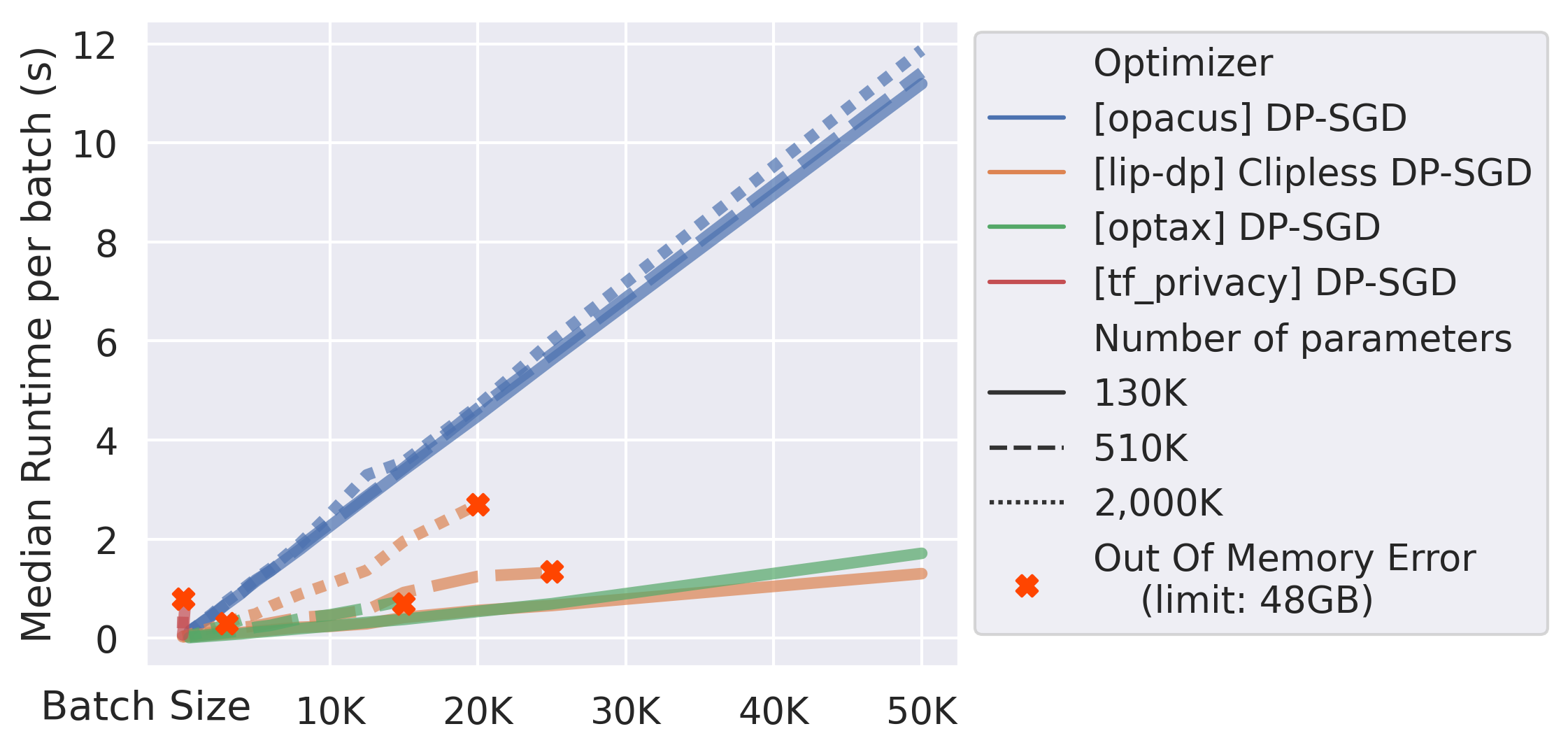
Figure 4: Our approach outperforms concurrent frameworks in terms of runtime and memory: we trained CNNs (ranging from 130K to 2M parameters) on CIFAR-10, and report the median batch processing time (including noise, and constraints application $\Pi$ or gradient clipping).

We benchmarked the median runtime per epoch of vanilla DP-SGD against the one of Clipless DP-SGD, on a CNN architecture and its Lipschitz equivalent respectively. The experiment was run on a GPU with 48GB video memory. We compare against the implementation of tf_privacy, opacus and optax. In order to allow a fair comparison, when evaluating Opacus, we reported the runtime with respect to the logical batch size, while capping the physical batch size to avoid Out Of Memory error (OOM). Although our library does not implement logical batching yet, it is fully compatible with this feature.

An advantage of projection $\Pi$ over per-sample gradient clipping is that the projection cost is independent of the batch size. Fig 4 validates that our method scales much better than vanilla DP-SGD, and is compatible with large batch sizes. It offers several advantages: firstly, a larger batch size contributes to a decrease of the sensitivity $\Delta\propto 1/b$, which diminishes the ratio between noise and gradient norm. Secondly, as the batch size $b$ increases, the variance decreases at the parametric rate $\mathcal{O}(\sqrt{b})$ (as demonstrated in appendix), aligning with expectations. This observation does not apply to DP-SGD: gradient clipping biases the direction of the average gradient, as noticed by [7].

Pareto front of privacy/utility trade-off.

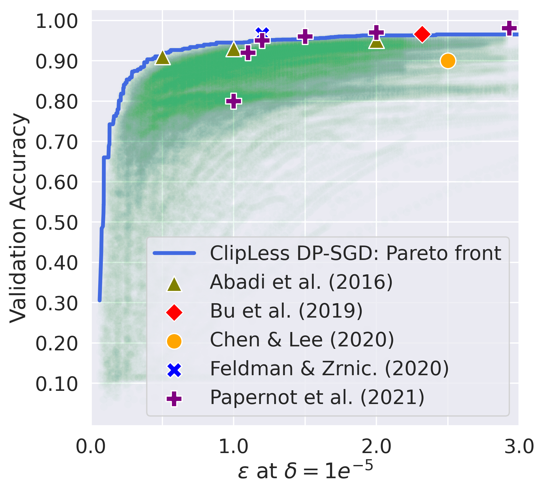
(a) MNIST.

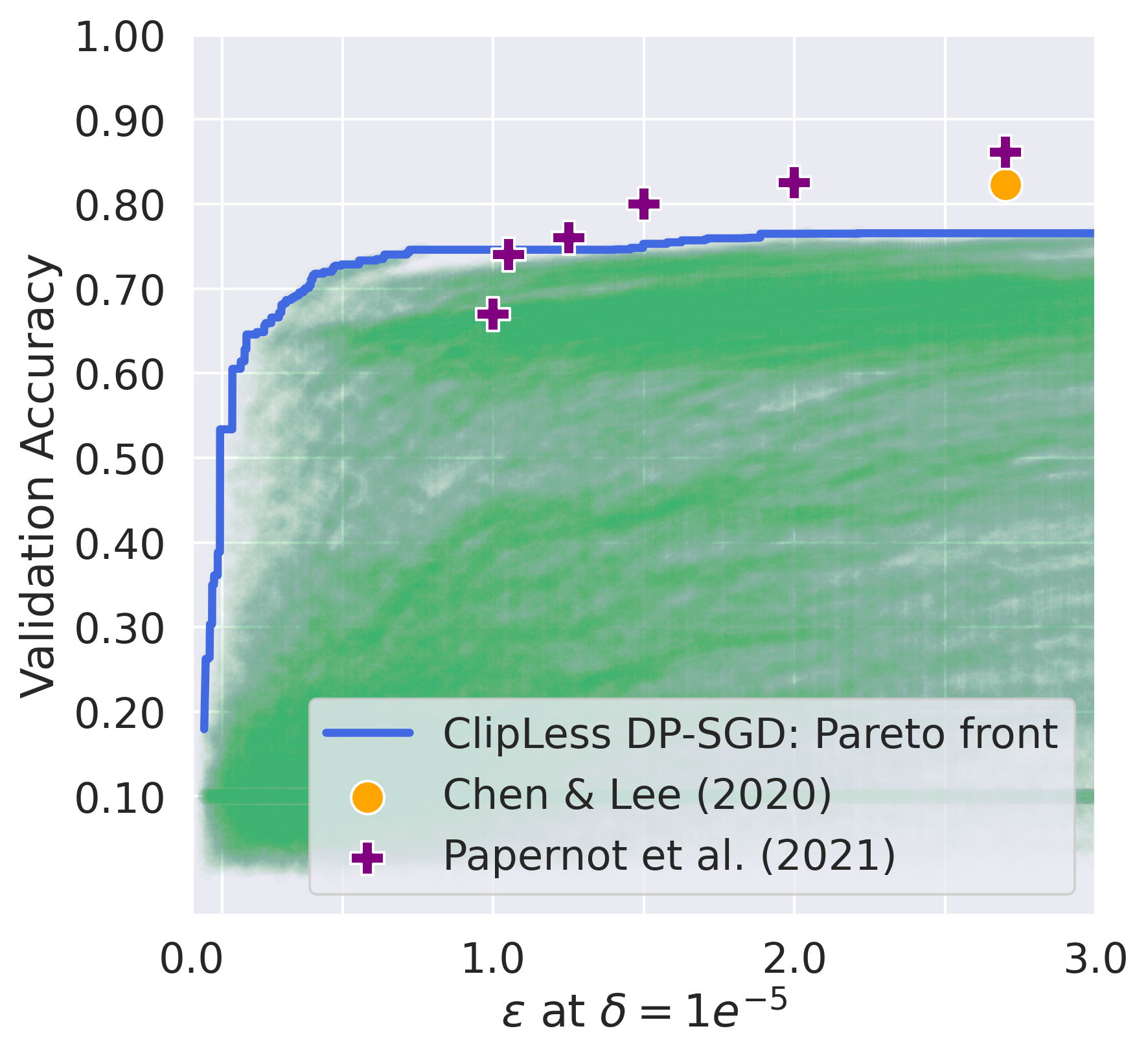
(b) F-MNIST.

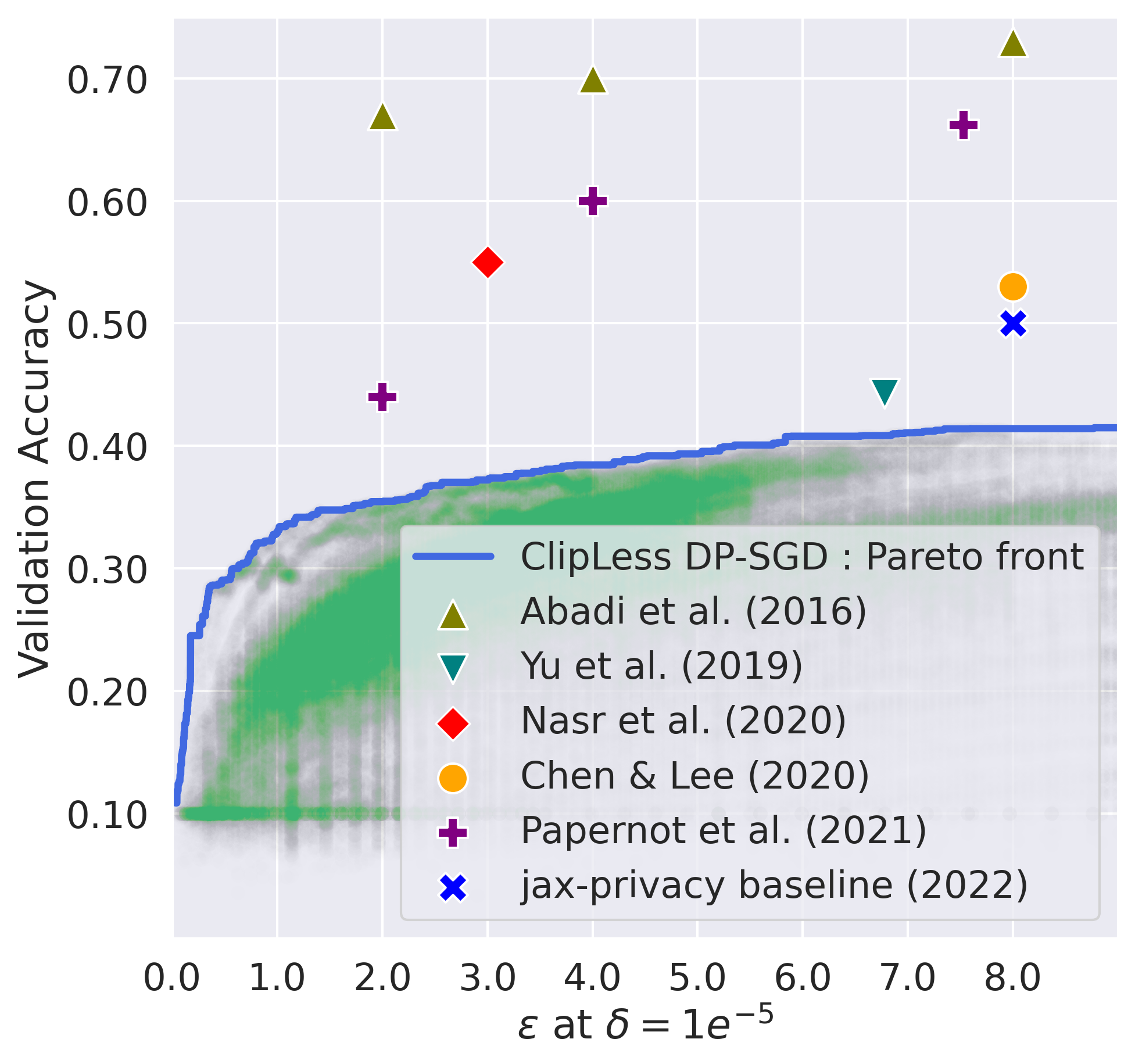
(c) CIFAR-10.

Figure 5: Our framework paints a clearer picture of the privacy/utility trade-off. We trained models in an "out of the box setting" (no pre-training, no data augmentation and no handcrafted features) on multiple tasks. While our results align with the baselines presented in other frameworks, we recognize the importance of domain-specific engineering. In this regard, we find the innovations introduced in  [49, 50, 51] and references therein highly relevant. These advancements demonstrate compatibility with our framework and hold potential for future integration.

We performed a search over a broad range of hyper-parameters values to cover the Pareto front between utility and privacy. Results are reported in Figure 5. We emphasize that our experiments did not use the elements behind the success of most recent papers (pre-training, data preparation, or handcrafted feature are examples). Hence our results are more representative of the typical performance that can be obtained in an “out of the box” setting. Future endeavors or domain-specific engineering can enhance the performance even further, but such improvements currently lie beyond the scope of our work. We also benchmarked architectures inspired from VGG [52], Resnet [53] and MLP_Mixers [54] see appendix for more details. Following standard practices of the community [2], we used sampling without replacement at each epoch (by shuffling examples), but we reported $\epsilon$ assuming Poisson sampling to benefit from privacy amplification [31]. We also ignore the privacy loss that may be induced by hyper-parameter search, which is a limitation per recent studies [5], but is common practice.

5 Limitations and future work

Although this framework offers a novel approach to address differentially private training, it introduces new challenges. We primary rely on GNP networks, where high performing architectures are quite different from the usual CNN architectures. As emphasized in Remark 2, we anticipate that progress in these areas would greatly enhance the effectiveness of our approach. Additionally, to meet requirement 3, we rely on projections, necessitating additional efforts to incorporate recent advancements associated with differentiable reparametrizations [42, 43]. It is worth noting that our methodology is applicable to most layers. Another limitation of our approach is the accurate computation of sensitivity $\Delta$, which is challenging due to the non-associativity of floating-point arithmetic and its impact on numerical stability [55]. This challenge is exacerbated on GPUs, where operations are inherently non-deterministic [56]. Finally, as mentioned in Remark 1, our propagation bound method can be refined.

6 Concluding remarks and broader impact

Besides its main focus on differential privacy, our work provides (1) a motivation to further develop Gradient Norm Preserving architectures. Furthermore, the development of networks with known Lipschitz constant with respect to parameters is a question of independent interest, (2) a useful tool for the study of the optimization dynamics in neural networks. Finally, Lipschitz networks are known to enjoy certificates against adversarial attacks [17, 57], and from generalization guarantees [13], without cost in accuracy [18]. We advocate for the spreading of their use in the context of robust and certifiable learning.

Appendix A Definitions and Methods

A.1 Additionnal background

The purpose of this appendix is to provide additionnal definitions and properties regarding Lipschitz Neural Networks, their possible GNP properties and Differential Privacy.

A.1.1 Lipschitz neural networks background

For simplicity of the exposure, we will focus on feedforward neural networks with densely connected layers: the affine transformation takes the form of a matrix-vector product $h\mapsto Wh$. In section C.2 we tackle the case of convolutions $h\mapsto\Psi*h$ with kernel $\Psi$.

Definition 4 (Feedforward neural network).

A feedforward neural network of depth $T$, with input space $\mathcal{X}\subset\mathbb{R}^{n}$, and with parameter space $\Theta\subset\mathbb{R}^{p}$, is a parameterized function $f:\Theta\times\mathcal{X}\rightarrow\mathcal{Y}$ defined by the following recursion:

$$h_{0}(x) \vcentcolon=x,\quad z_{t}(x) \vcentcolon=W_{t}h_{t-1}(x)+b_{t},$$

$$h_{t}(x) \vcentcolon=\sigma(z_{t}(x)),\quad f(\theta,x) \vcentcolon=z_{T+1}(x).$$ (8)

The set of parameters is denoted as $\theta=(W_{t},b_{t})_{1\leq t\leq T+1}$, the output space as $\mathcal{Y}\subset\mathbb{R}^{K}$ (e.g logits), and the layer-wise activation as $\sigma:\mathbb{R}^{n}\rightarrow\mathbb{R}^{n}$.

Definition 5 (Lipschitz constant).

The function $f:\mathbb{R}^{m}\rightarrow\mathbb{R}^{n}$ is said $l$-Lipschitz for $l_{2}$ norm if for every $x,y\in\mathbb{R}^{m}$ we have:

$$\|f(x)-f(y)\|_{2}\leq l\|x-y\|_{2}.$$ (9)

Per Rademacher’s theorem [10], its gradient is bounded: $\|\nabla f\|\leq l$. Reciprocally, continuous functions gradient bounded by $l$ are $l$-Lipschitz.

Definition 6 (Lipschitz neural network).

A Lipschitz neural network is a feedforward neural network with the additional constraints:

• the activation function $\sigma$ is $S$-Lipschitz. This is a standard assumption, frequently fulfilled in practice.

• the affine functions $x\mapsto Wx+b$ are $U$-Lipschitz, i.e $\|W\|_{2}\leq U$. This is achieved in practice with spectrally normalized matrices [12] [13]. The feasible set is the ball $\{\|W\|_{2}\leq U\}$ of radius $U$ (which is convex), or a subset of thereof (not necessarily convex).

As a result, the function $x\mapsto f(\theta,x)$ is $U(US)^{T}$-Lipschitz for all $\theta\in\Theta$.

Two strategies are available to enforce Lipschitzness:

1. With a differentiable reparametrization $\Pi:\mathbb{R}^{p}\rightarrow\Theta$ where $\tilde{\theta}=\Pi(\theta)$: the weights $\tilde{\theta}$ are used during the forward pass, but the gradients are back-propagated to $\theta$ through $\Pi$. This turns the training into an unconstrained optimization problem on the landscape of $\mathcal{L}\circ f\circ\Pi$.

2. With a suitable projection operator $\Pi:\mathbb{R}^{p}\rightarrow\Theta$: this is the celebrated Projected Gradient Descent (PGD) algorithm [58] applied on the landscape of $\mathcal{L}\circ f$.

For arbitrary re-parametrizations, option 1 can cause some difficulties: the Lipschiz constant of $\Pi$ is generally unknown. However, if $\Theta$ is convex then $\Pi$ is 1-Lipschitz (with respect to the norm chosen for the projection). To the contrary, option 2 elicits a broader set of feasible sets $\Theta$. For simplicity, option 2 will be the focus of our work.

A.1.2 Gradient Norm Preserving networks

Definition 7 (Gradient Norm Preserving Networks).

GNP networks are 1-Lipschitz neural networks with the additional constraint that the Jacobian of layers consists of orthogonal matrices:

$$\left(\frac{\partial f_{d}}{\partial x_{d}}\right)^{T}\left(\frac{\partial f_{d}}{\partial x_{d}}\right)=I.$$ (10)

This is achieved with GroupSort activation [8, 39], Householder activation [40], and orthogonal weight matrices [17, 41] or orthogonal convolutions (see [44, 45, 46] and references therein). Without biases these networks are also norm preserving: $\|f(\theta,x)\|=\|x\|.$

The set of orthogonal matrices (and its generalization the Stiefel manifold [20]) is not convex, and not even connected. Hence projected gradient approaches are mandatory: for re-parametrization methods the Jacobian $\frac{\partial\Pi}{\partial\theta}$ may be unbounded which could have uncontrollable consequences on sensitivity.

A.1.3 Differential Privacy background

Definition 8 (Neighboring datasets).

A labelled dataset $\mathcal{D}$ is a finite collection of input/label pairs $\mathcal{D}=\{(x_{1},y_{1}),(x_{2},y_{2}),\ldots...(x_{N},y_{N})\}$. Two datasets $\mathcal{D}$ and $\mathcal{D}^{\prime}$ are said to be neighbouring if they differ by at most one sample: $\mathcal{D}^{\prime}=\mathcal{D}\cup\{(x^{\prime},y^{\prime})\}-\{(x_{i},y_{i})\}$.

The sensitivity is also referred as algorithmic stability [59], or bounded differences property in other fields [60]. We detail below the building of a Gaussian mechanism from an arbitrary query of known sensitivity.

Definition 9 (Gaussian Mechanism).

Let $f:\mathcal{D}\rightarrow\mathbb{R}^{p}$ be a query accessing the dataset of known $l_{2}$-sensitivity $\Delta(f)$, a Gaussian mechanism adds noise sampled from $\mathcal{N}(0,\sigma.\Delta(f))$ to the query $f$.

Property 1 (DP of Gaussian Mechanisms).

Let $\mathcal{G}(f).$ be a Gaussian mechanism of $l_{2}$-sensitivity $S_{2}(f)$ adding the noise $\mathcal{N}(0,\sigma.S_{2}(f))$ to the query $f$. The DP guarantees of the mechanism are given by the following continuum: $\sigma=\sqrt{2.\log(1.25/\delta)}/\epsilon.$

SGD is a composition of queries. Each of those query consists of sampling a minibatch from the dataset, and computing the gradient of the loss on the minibatch. The sensitivity of the query is proportional to the maximum gradient norm $l$, and inversely proportional to the batch size $b$. By pertubing the gradient with a Gaussian noise of variance $\sigma^{2}\frac{l^{2}}{b^{2}}$ the query is transformed into a Gaussian mechanism. By composing the Gaussian mechanisms we obtain the DPSGD variant, that enjoy $(\epsilon,\delta)$-DP guarantees.

Proposition 1 (DP guarantees for SGD, adapted from [1].).

Assume that the loss fulfills $\|\nabla_{\theta}\mathcal{L}(\hat{y},y)\|_{2}\leq l$, and assume that the network is trained on a dataset of size $N$ with SGD algorithm for $T$ steps with noise scale $\mathcal{N}(\bf 0,\sigma^{2})$ such that:

$$\sigma\geq\frac{16K\sqrt{T\log{(2/\delta)}\log{(1.25T/\delta N)}}}{N\epsilon}.$$ (11)

Then the SGD training of the network is $(\epsilon,\delta)$-DP.

A.2 More about Clipless DP-SGD

About the “local” strategy.

Illustrated in Figures 3. We dissect the DP-mechanism that consists of the SGD steps applied on each layer. Indeed, we are able to characterise the sensitivity $\Delta_{d}$ of every layer of the network. Therefore, we give $(\epsilon_{d},\delta_{d})$-DP guarantees on a per-layer basis. Finally however, we would still have to be able to guarantee $(\epsilon,\delta)$-DP on the whole model.

1. On each layer, we apply a Gaussian mechanism [9] with noise variance $\sigma^{2}\Delta_{d}^{2}$.

2. Their composition yields an other Gaussian mechanism with non isotropic noise.

3. The Gaussian mechanism benefits from privacy amplification via subsampling [31] thanks to the stochasticity in the selection of batches of size $b=pN$.

4. Finally an epoch is defined as the composition of $T=\frac{1}{p}$ sub-sampled mechanisms.

Different layers exhibit different maximum gradient bounds - and in turn this implies different sensitivities. This also suggests that different noise multipliers $\sigma_{d}$ can be used for each layer. This open extensions for future work.

We detail in Algorithm 3 the global variant of our approach.

Algorithm 3 Clipless DP-SGD with global sensitivity accounting

Input: Feed-forward architecture $f(\cdot,\cdot)=f_{T+1}(\Theta_{T+1},\cdot)\circ f_{T}(\Theta_{T},\cdot)\circ\ldots\circ f_{0}(\Theta_{0},\cdot)$
Input: Initial weights $\theta_{0}$, learning rate scheduling $\eta_{t}$, noise multiplier $\sigma$.

1:repeat

2:     $\Delta_{0}\ldots\Delta_{T+1}\leftarrow$ compute_gradient_bounds$(f,X).$

3:     Sample a batch $\mathcal{B}_{t}=\{(x_{1},y_{1}),(x_{2},y_{2}),\ldots,(x_{b},y_{b})\}$.

4:     Compute the mean gradient of the batch for each layer $t$:

$$\tilde{g}_{t}\vcentcolon=\frac{1}{b}\sum_{i=1}^{b}\nabla_{W_{t}}\mathcal{L}(\hat{y}_{i},y_{i})).$$

5:     For each layer $t$ of the model, get the theoretical bound of the gradient:

$$\forall 1\leq i\leq b,\quad\|\nabla_{W_{t}}\mathcal{L}(\hat{y}_{i},y_{i})\|_{2}\leq\Delta_{t}.$$

6:     Update Moment accountant state with global sensivity $\Delta=\frac{2}{b}\sqrt{\sum_{t=1}^{T+1}\Delta_{t}^{2}}$.

7:     Add global noise $\zeta\sim\mathcal{N}(0,2\sigma\Delta/b)$ to each weights and perform projected gradient step:

$$W_{t}\leftarrow\Pi(W_{t}-\eta(\tilde{g}_{t}+\zeta)).$$

8:     Report new $(\epsilon,\delta)$-DP guarantees with accountant.

9:until privacy budget $(\epsilon,\delta)$ has been reached.

Appendix B Lipdp tutorial

This section gives advice on how to start your DP training processes using the framework. Moreover, it provides insights into how input pre-processing, building networks with Residual connections and Loss-logits gradient clipping could help offer better utility for the same privacy budget.

B.1 Prerequisite: building a $l$-Lipschitz network

As per def 3 a $l$-Lipschitz neural network of depth $d$ can be built by composing $\sqrt[d]{l}$ layers. In the rest of this section we will focus on 1-Lipschitz networks (rather than controlling $l$ we control the loss to obtain the same effects [18]). In order to do so the strategy consists in choosing only 1-Lipschitz activations, and to constrain the weights of parameterized layers such that it can only express 1-Lipschitz functions. For instance normalizing the weight matrix of a dense layer by its spectral norm yield a 1-Lipschitz layer (this, however cannot be applied trivially on convolution’s kernel). In practice we used the layers available in the open-source library deel-lip. In practice, when building a Lipschitz network, the following block can be used:

• Dense layers: are available as SpectralDense or QuickSpectralDense which apply spectral normalization and Björck orthogonalization (for GNP layers).

• Relu activations are replaced by Groupsort2 activations, and such activations are GNP, preventing vanishing gradient.

• pooling layers are replaced with ScaledL2NormPooling, which is GNP.

• normalization layers like BatchNorm are not $K$-Lipschitz. We did not accounted these layers since they can induce a privacy leak (as they keep a rolling mean and variance). A 1-Lipschitz drop-in replacement is studied in C.2.3. The relevant literature also propose drop-in replacement for this layer with proper sensitivity accounting.

Originally, this library relied on differentiable re-parametrizations, since it yields higher accuracy outside DP training regime (clean training without noise). However, our framework does not account for the Lipschitz constant of the re-parametrization operator. This is why we provide QuickSpectralDense and QuickSpectralConv2D layers to enforce Lipschitz constraints, where the projection is enforced with a tensorflow constraint. Note that SpectralDense and SpectralConv2D can still be used with a CondenseCallack to enforce the projection, and bypass the back-propagation through the differentiable re-parametrization. However this last solution, while being closer to the original spirit of deel-lip, is also less efficient in speed benchmarks.

The Lipschitz constant of each layer is bounded by $1$, since each weight matrix is divided by the largest singular value $\sigma_{\text{max}}$. This singular value is computed with Power Iteration algorithm. Power Iteration computes the largest singular value by repeatedly computing a Rayleigh quotient asssociated to a vector $u$, and this vector eventually converges to the eigenvector $u_{\max}$ associated to the largest eigenvalue. These iterations can be expensive. However, since gradient steps are smalls, the weight matrices $W_{t}$ and $W_{t+1}$ remain close to each other after a gradient step. Hence their largest eigenvectors tend to be similar. Therefore, the eigenvector $u_{\max}$ can be memorized at the end of each train step, and re-used as high quality initialization at the next train step, in a “lazy” fashion. This speed-up makes the overall projection algorithm very efficient.

B.2 Getting started

The framework we propose is built to allow DP training of neural networks in a fast and controlled approach. The tools we provide are the following :

1. A pipeline to efficiently load and pre-process the data of commonly used datasets like MNIST, FashionMNIST and CIFAR10.

2. Configuration objects to correctly account DP events we provide config objects to fill in that will

3. Model objects on the principle of Keras’ model classes we offer both a DP_Model and a DP_Sequential class to streamline the training process.

4. Layer objects where we offer a readily available form of the principal layers used for DNNs. These layers are already Lipschitz constrained and possess class specific methods to access their Lipschitz constant.

5. Loss functions, identically, we offer DP loss functions that automatically compute their Lipschitz constant for correct DP enforcing.

We highlight below an example of a full training loop on Mnist with lip-dp library. Refer to the “examples” folder in the library for more detailed explanations in a jupyter notebook.

⬇

dp_parameters = DPParameters(

noisify_strategy="global",

noise_multiplier=2.0,

delta=1e-5,

)

epsilon_max = 3.0

input_upper_bound = 20.0

ds_train, ds_test, dataset_metadata = load_and_prepare_data(

"mnist",

batch_size=1000,

drop_remainder=True,

bound_fct=bound_clip_value(

input_upper_bound

),

)

# construct DP_Sequential

model = DP_Sequential(

layers=[

layers.DP_BoundedInput(

input_shape=dataset_metadata.input_shape, upper_bound=input_upper_bound

),

layers.DP_QuickSpectralConv2D(

filters=32,

kernel_size=3,

kernel_initializer="orthogonal",

strides=1,

use_bias=False,

),

layers.DP_GroupSort(2),

layers.DP_ScaledL2NormPooling2D(pool_size=2, strides=2),

layers.DP_QuickSpectralConv2D(

filters=64,

kernel_size=3,

kernel_initializer="orthogonal",

strides=1,

use_bias=False,

),

layers.DP_GroupSort(2),

layers.DP_ScaledL2NormPooling2D(pool_size=2, strides=2),

layers.DP_Flatten(),

layers.DP_QuickSpectralDense(512),

layers.DP_GroupSort(2),

layers.DP_QuickSpectralDense(dataset_metadata.nb_classes),

],

dp_parameters=dp_parameters,

dataset_metadata=dataset_metadata,

)

model.compile(

loss=losses.DP_TauCategoricalCrossentropy(18.0),

optimizer=tf.keras.optimizers.SGD(learning_rate=2e-4, momentum=0.9),

metrics=["accuracy"],

)

model.summary()

num_epochs = get_max_epochs(epsilon_max, model)

hist = model.fit(

ds_train,

epochs=num_epochs,

validation_data=ds_test,

callbacks=[

# accounting is done thanks to a callback

DP_Accountant(log_fn="logging"),

],

)

B.3 Image spaces and input clipping

Input preprocessing can be done in a completely dataset agnostic way and may yield positive results on the models utility. We explore here the choice of the color space, and the norm clipping of the input.

B.3.1 Color space representations

The color space representation of the color images of the CIFAR10 dataset for example can yield very different gradient norms during the training process. Therefore, we can take advantage of this to train our DP models more efficiently. Empirically, Figures 6(a) and 6(b) show that some color spaces yield narrower image norm distributions that happen to be more advantageous to maximise the mean gradient norm to noise ratio across all samples during the DP training process of GNP networks.

B.3.2 Input clipping

A clever way to narrow down the distribution of the dataset’s norms would be to clip the norms of the input of the model. This may result in improved utility since a narrower distribution of input norms might maximise the mean gradient norm to noise ratio for misclassified examples. Also, we advocate for the use of GNP networks as their gradients usually turn out to be closer to the upper bound we are able to compute for the gradient. See Figure 7(a) and 7(b)

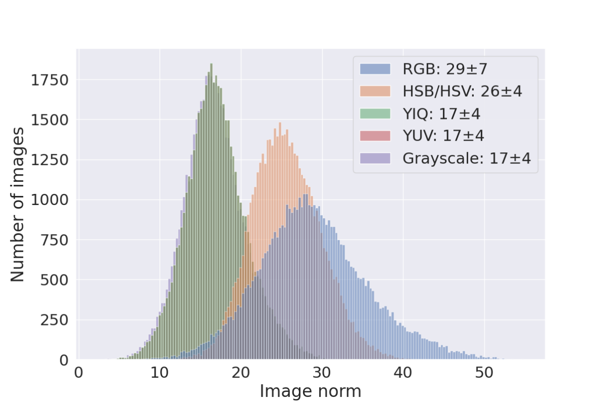
(a) Input norms.

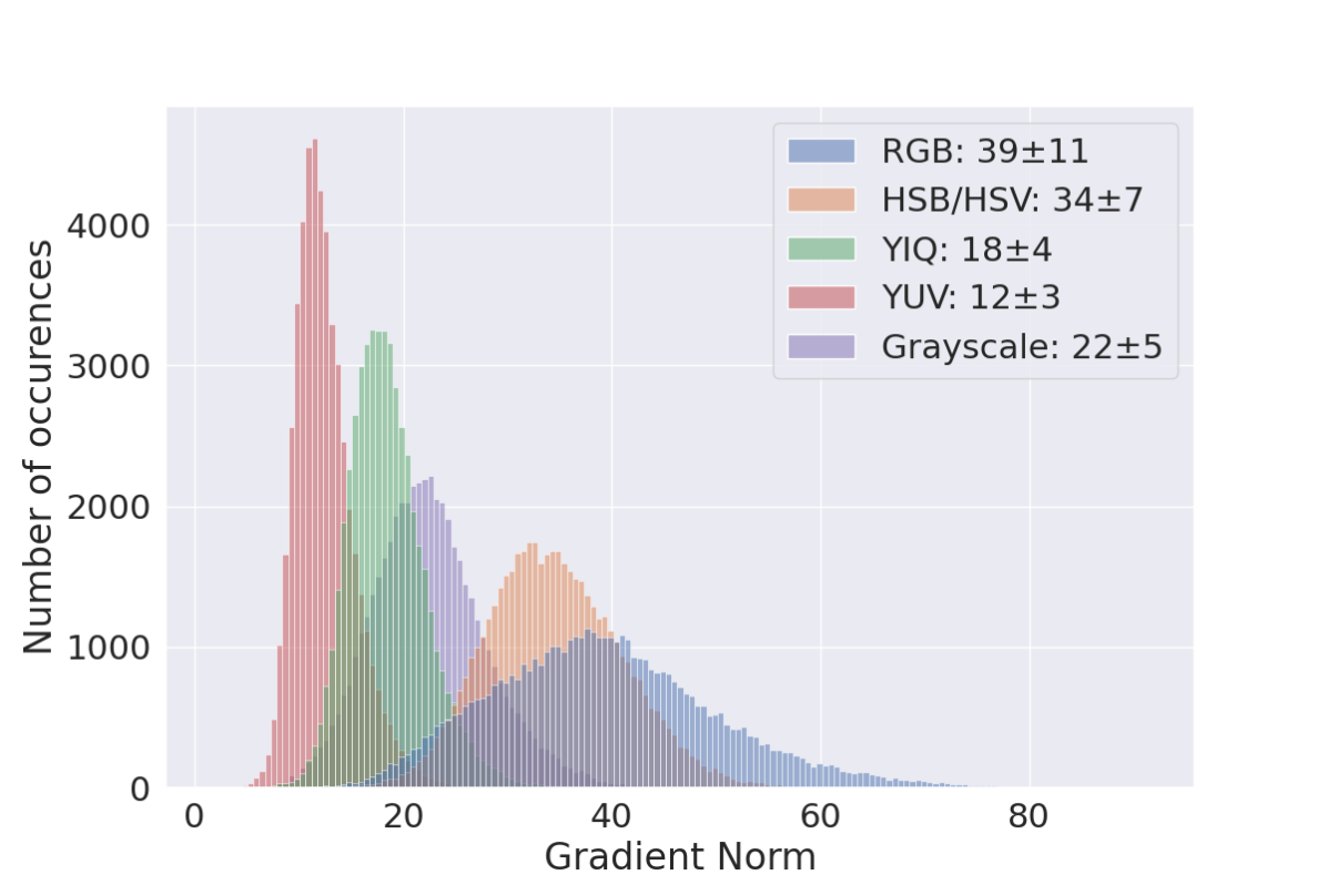
(b) Gradient norms.

Figure 6: Histogram of norms for different image space on CIFAR-10 images. We see that for GNP networks the distribution of dataset norms have a strong influence on the norm of the individual parameterwise gradient norms of missclassified examples.

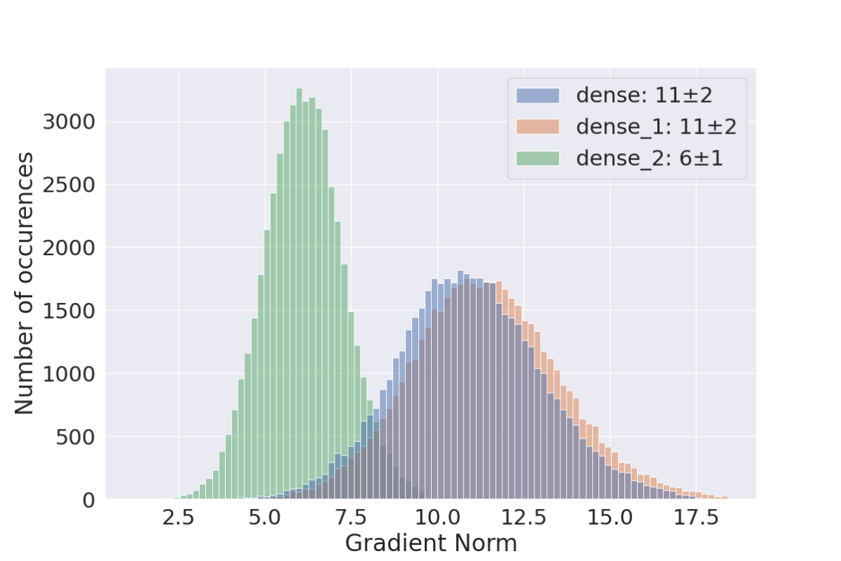
(a) Conventional network.

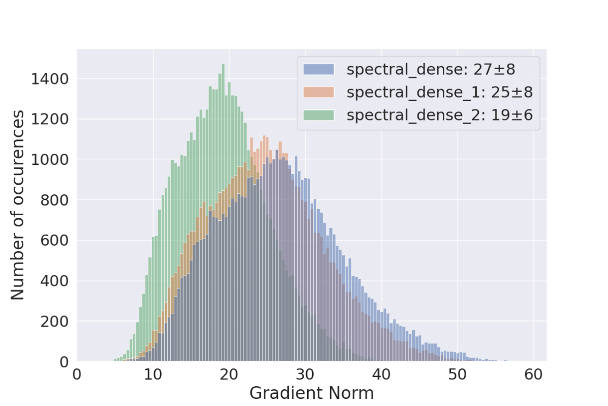
(b) Gradient Norm Preserving network.

Figure 7: Gradient norms of fully-connected networks on CIFAR-10. We see that GNP networks exhibit a qualitatively different profile of gradient norms with respect to parameters, sticking closer to the upper bound we are able to compute for the gradient norm.

B.4 Practical implementation of Residual connections

The implementation of skip connections is made relatively straightforward in our framework by the make_residuals method. This function splits the input path in two, and wraps the layers inside the residual connections, as illustrated in figure 8.

⬇

from lipdp.layers import make_residuals

## Manual implementation of residual connection:

layers = [DP_SplitResidual(),

DP_WrappedResidual(DP_QuickSpectralConv2D(16, (3, 3)),

DP_WrappedResidual(DP_GroupSort(2)),

DP_MergeResidual(’1-lip-add’)]

## Or equivalently, with helper function:

layers = make_residuals([

DP_QuickSpectralConv2D(16, (3, 3),

DP_GroupSort(2)

])

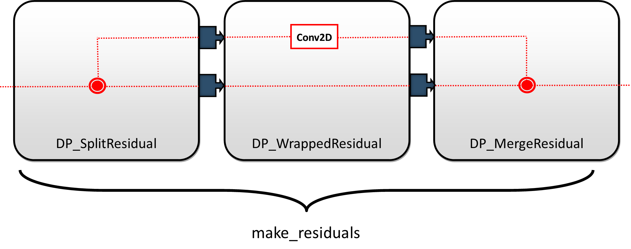
Figure 8: Implementation of a skip connection in the lip-dp framework. The meta block DP_WrappedResidual handle the forward propagation and the backward propagation of pairs of bounds (one for each computation path) by leveraging the forward and the backward of sub-blocks. DP_SplitResidual handle the creation of a tuple of input bounds at the forward, and collapse the tuple of gradient bounds into a scalar at the backward, while DP_MergeResidual does the opposite. All those operations are wrapped under the convenience function make_residuals.

By using this implementation, the sensitivity of the gradient computation and the input bounds to each layer are correctly computed when the model’s path is split. This allows for fairly easy implementations of models like the MLP-Mixer and ResNets. Since convolutional models may suffer from gradient vanishing and that dense based models are relatively restrictive in terms of architecture, implementing skip connections could be a useful feature for our framework.

B.5 Loss-logits gradient clipping

The advantage of the traditional DP-SGD approach is that through hyperparameter optimization on the global gradient clipping constant, we indirectly optimize the mean signal to noise ratio on missclassified examples. However, this clipping constant is not really explainable and rather just an empirical result of optimization on a given architecture and loss function.

Importantly, our framework is compatible with a more efficient and explainable form of clipping. Indeed, by introducing a gradient clipping layer in our framework we are able to clip the gradient of the loss on the final logits for a minimal cost.

Indeed, in this case the size of the clipped vector is the output dimension $|\hat{y}|$, which is small for a lot of practical regression and classification tasks. For example in CIFAR-10 the output vector is of length $10$. This scales better with the batch size than the weight matrices that are typically of sizes ${64\times 64}$ or ${128\times 128}$.

Note that this clipping value can also follow a scheduling during training, in the spirit of [61] - but care must be taken that the scheduling is either data independent, or in the case it is data dependant the privacy leaks must be taken into account. The implementation of loss gradient clipping scheduling is yet to be implemented in our framework. However, it is expected to be a part of future works.

Furthermore, if the gradient clipping layer is inserted on the tail of the network (between the logits and the loss) we can characterize its effects on the training, in particular for classification tasks with binary cross-entropy loss.

We denote by $\mathcal{L}(\text{Clip}^{C}_{\nabla}(\hat{y}))$ the loss wrapped under a DP_ClipGradient layer that behaves like identity $x\mapsto x$ at the forward, and clips the gradient norm to $C>0$ in the backward pass:

$$\nabla_{\hat{y}}\left(\mathcal{L}(\text{Clip}^{C}_{\nabla}(\hat{y}))\right)\vcentcolon= \min{(1,\frac{C}{\|\nabla_{\hat{y}}\mathcal{L}(\hat{y})\|})}\nabla_{\hat{y}}\mathcal{L}(\hat{y})$$ (12)

$$= \min{(\|\nabla_{\hat{y}}\mathcal{L}(\hat{y})\|,C)}\frac{\nabla_{\hat{y}}\mathcal{L}(\hat{y})}{\|\nabla_{\hat{y}}\mathcal{L}(\hat{y})\|}.$$ (13)

We denote by $\overrightarrow{g(\hat{y})}$ the unit norm vector $\frac{\nabla_{\hat{y}}\mathcal{L}(\hat{y})}{\|\nabla_{\hat{y}}\mathcal{L}(\hat{y})\|}$. Then:

$$\nabla_{\hat{y}}\left(\mathcal{L}(\text{Clip}^{C}_{\nabla}(\hat{y}))\right)=\min{(\|\nabla_{\hat{y}}\mathcal{L}(\hat{y})\|,C)}\overrightarrow{g(\hat{y})}.$$

Proposition 2 (Clipped binary cross-entropy loss is the Wasserstein dual loss).

Let $\mathcal{L}_{BCE}(\hat{y},y)=-\log{(\sigma(\hat{y}y))}$ be the binary cross-entropy loss, with $\sigma(\hat{y}y)=\frac{1}{1+\exp{(-\hat{y}y)}}$ the sigmoid activation, assuming discrete labels ${y\in\{-1,+1\}}$. Assume examples are sampled from the dataset $\mathcal{D}$. Let $\hat{y}(\theta,x)=f(\theta,x)$ be the predictions at input $x\in\mathcal{D}$. Then for every $C>0$ sufficiently small, a gradient descent step with the clipped gradient $\nabla_{\theta}\mathbb{E}_{\mathcal{D}}[\mathcal{L}(\text{Clip}^{C}_{\nabla}(\hat{y},y))]$ is identical to the gradient ascent step obtained from Kantorovich-Rubinstein loss $\mathcal{L}_{KR}(\hat{y},y)=\hat{y}y$.

Proof.

In the following we use the short notation $\mathcal{L}$ in place of $\mathcal{L}_{BCE}$. Assume that examples with labels $+1$ (resp. $-1$) are sampled from distribution $P$ (resp. $Q$). By definition:

$$\nabla_{\theta}\mathbb{E}_{\mathcal{D}}[\mathcal{L}(\text{Clip}^{C}_{\nabla}(\hat{y},y))]=\nabla_{\theta}\left(\mathbb{E}_{x\sim P}[\mathcal{L}(\text{Clip}^{C}_{\nabla}(f(\theta,x),+1))]+\mathbb{E}_{x\sim Q}[\mathcal{L}(\text{Clip}^{C}_{\nabla}(f(\theta,x),-1))]\right).$$

Observe that the output of the network is a single scalar, hence $\overrightarrow{g(\hat{y})}\in\{-1,+1\}$. We apply the chainrule $\nabla_{\theta}\mathcal{L}=\nabla_{\hat{y}}\mathcal{L}\frac{\partial\hat{y}}{\partial\theta}=\overrightarrow{g(\hat{y})}\min{(\|\nabla_{\hat{y}}\mathcal{L}(\hat{y})\|,C)}\nabla_{\theta}f(\theta,x)$. We note $R(\hat{y},C)\vcentcolon=\min{(\|\nabla_{\hat{y}}\mathcal{L}(\hat{y})\|,C)}>0$ and we obtain:

$$\nabla_{\theta}\mathbb{E}_{\mathcal{D}}[\mathcal{L}(\text{Clip}^{C}_{\nabla}(\hat{y},y))]=\nabla_{\theta}\left(\mathbb{E}_{x\sim P}[\overrightarrow{g(\hat{y})}R(\hat{y},C)\nabla_{\theta}f(\theta,x)]+\mathbb{E}_{x\sim Q}[\overrightarrow{g(\hat{y})}R(\hat{y},C)\nabla_{\theta}f(\theta,x)]\right).$$ (14)

Observe that the value of $\overrightarrow{g(\hat{y})}$ can actually be deduced from the label $y$, which gives:

$$\nabla_{\theta}\mathbb{E}_{\mathcal{D}}[\mathcal{L}(\hat{y},y)]=-\mathbb{E}_{x\sim P}[R(\hat{y},C)\nabla_{\theta}f(\theta,x)]+\mathbb{E}_{x\sim Q}[R(\hat{y},C)\nabla_{\theta}f(\theta,x)].$$ (15)

Observe that the function $x\mapsto\nabla_{\hat{y}}\mathcal{L}(\hat{y})$ is piecewise-continuous when the loss $\hat{y}\mapsto\mathcal{L}(\hat{y},y)$ is piecewise continuous. Observe that $|\nabla_{\hat{y}}\mathcal{L}(\hat{y})|$ is non zero, since the loss $\mathcal{L}$ does not achieve its minimum over the open set $(-\infty,+\infty)$, since $\sigma(\hat{y})\in(0,1)$. Assuming that the data $x\in\mathcal{D}$ live in a compact (or equivalently that $P$ and $Q$ have compact support), since $x\mapsto|\nabla_{\hat{y}}\mathcal{L}(\hat{y})|$ is piecewise continuous (with finite number of pieces for finite neural networks) it attains its minimum $C^{\prime}>0$. Choosing any $C<C^{\prime}$ implies that $R(\hat{y},C)=C$, which yields:

$$\nabla_{\theta}\mathbb{E}_{\mathcal{D}}[\mathcal{L}(\text{Clip}^{C}_{\nabla}(\hat{y},y))] =-\mathbb{E}_{x\sim P}[C\nabla_{\theta}f(\theta,x)]+\mathbb{E}_{x\sim Q}[C\nabla_{\theta}f(\theta,x)]$$

$$=-C\left(\mathbb{E}_{x\sim P}[\nabla_{\theta}f(\theta,x)]-\mathbb{E}_{x\sim Q}[\nabla_{\theta}f(\theta,x)]\right).$$

This corresponds to a gradient ascent step of length $C$ on the Kantorovich-Rubinstein (KR) objective $\mathcal{L}_{KR}(\hat{y},y)=\hat{y}y$. This loss is named after the Kantorovich Rubinstein duality that arises in optimal transport, than states that the Wasserstein-1 distance is a supremum over 1-Lipschitz functions:

$$\mathcal{W}_{1}(P,Q)\vcentcolon=\underset{f\in\text{1-Lip}(\mathcal{D},\mathbb{R})}{\sup}\mathbb{E}_{x\sim P}[f(x)]-\mathbb{E}_{x\sim Q}[f(x)].$$ (16)

Hence, with clipping $C$ small enough the gradient steps are actually identical to the ones performed during the estimation of Wasserstein-1 distance. ∎

In future works, other multi-class losses can be studied through the lens of per-example clipping. Our framework permits the use of gradient clipping while at the same time faciliting the theoretical anaysis.

B.5.1 Possible improvements

Our framework is compatible with possible improvements in methods of data pre-processing. For instance some works suggest that feature engineering is the key to achieve correct utility/privacy trade-off [50] some other work rely on heavily over-parametrized networks, coupled with batch size [51]. While we focused on providing competitive and reproducible baselines (involving minimal pre-processing and affordable compute budget) our work is fully compatible with those improvements. Secondly the field of GNP networks (also called orthogonal networks) is still an active field, and new methods to build better GNP networks will improve the efficiency of our framework ( for instance orthogonal convolutions [44],[41],[17],[42],[43] are still an active topic). Finally some optimizations specific to our framework can also be developed: a scheduling of loss-logits clipping might allow for better utility scores by following the declining value of the gradient of the loss, therefore allowing for a better mean signal to noise ratio across a diminishing number of miss-classified examples.

Appendix C Computing Sensitivity Bounds

C.1 Losses bounds

Loss	Hyper-parameters	$\mathcal{L}(\hat{y},y)$	Lipschitz bound $L$
Softmax Cross-entropy	temperature $\tau>0$	$y^{T}\log{\text{softmax}(\hat{y}/\tau)}$	$\sqrt{2}/\tau$
Cosine Similarity	bound $X_{\text{min}}>0$	$\frac{y^{T}\hat{y}}{\max(\|\hat{y}\|,X_{\text{min}}}$	$1/X_{\text{min}}$
Multiclass Hinge	margin $m>0$	$\{\text{max}(0,\frac{m}{2}-\hat{y}_{i}.y_{i})\}_{1\leq i\leq K}$	1
Kantorovich-Rubenstein	N/A	$\{\hat{y},y\}$	1
Hinge Kantorovich-Rubenstein	margin $m>0$ regularization $\alpha>0$	$\alpha.\mathcal{L}_{MH}(\hat{y},y)+\mathcal{L}_{MKR}(\hat{y},y)$	$1+\alpha$

Table 1: Lipschitz constant of common supervised classification losses used for the training of Lipschitz neural networks with $k$ classes. Proofs in section C.1.

This section contains the proofs related to the content of table 1. Our framework wraps over some losses found in deel-lip library, that are wrapped by our framework to provide Lipschitz constant automatically during backpropagation for bounds.

Multiclass Hinge

This loss, with min margin $m$ is computed in the following manner for a one-hot encoded ground truth vector $y$ and a logit prediction $\hat{y}$ :

$$\mathcal{L}_{MH}(\hat{y},y)=\{\max(0,\frac{m}{2}-\hat{y}_{1}.y_{1}),...,\max(0,\frac{m}{2}-\hat{y}_{k}.y_{k})\}.$$

And $\|\frac{\partial}{\partial y}\mathcal{L}_{MH}(\hat{y},y)\|_{2}\leq\|\hat{y}\|_{2}$. Therefore $L_{H}=1$.

Multiclass Kantorovich Rubenstein

This loss, is computed in a one-versus all manner, for a one-hot encoded ground truth vector $y$ and a logit prediction $\hat{y}$ :

$$\mathcal{L}_{MKR}(\hat{y},y)=\{\hat{y}_{1}-y_{1},\ldots,\hat{y}_{k}-y_{k})\}.$$

Therefore, by differentiating, we also get $L_{KR}=1$.

Multiclass Hinge - Kantorovitch Rubenstein

This loss, is computed in the following manner for a one-hot encoded ground truth vector $y$ and a logit prediction $\hat{y}$ :

$$\mathcal{L}_{MHKR}(\hat{y},y)=\alpha\mathcal{L}_{MH}(\hat{y},y)+\mathcal{L}_{MKR}(\hat{y},y).$$

By linearity we get $L_{HKR}=\alpha+1$.

Cosine Similarity

Cosine Similarity is defined in the following manner element-wise :

$$\mathcal{L}_{CS}(\hat{y},y)=\frac{\hat{y}^{T}y}{\|\hat{y}\|_{2}\|y\|_{2}}.$$

And $y$ is one-hot encoded, therefore $\mathcal{L}_{CS}(\hat{y},y)=\frac{\hat{y_{i}}}{\|\hat{y}\|_{2}}$. Therefore, the Lipschitz constant of this loss is dependant on the minimum value of $\hat{y}$. A reasonable assumption would be $\forall x\in\mathcal{D}$ : $X_{min}\leq\|x\|_{2}\leq X_{max}$. Furthermore, if the networks are Norm Preserving with factor K, we ensure that:

$$KX_{min}\leq\|\hat{y}\|_{2}\leq KX_{max}.$$

Which yields: $L_{CS}=\frac{1}{KX_{min}}$. The issue is that the exact value of $K$ is never known in advance since Lipschitz networks are rarely purely Norm Preserving in practice due to various effects (lack of tightness in convolutions, or rectangular matrices that can not be perfectly orthogonal).

Realistically, we propose the following loss function in replacement:

$$\mathcal{L}_{K-CS}(\hat{y},y)=\frac{\hat{y_{i}}}{\max(KX_{min},\|\hat{y}\|_{2})}.$$

Where $K$ is an input given by the user, therefore enforcing $L_{K-CS}=\frac{1}{KX_{min}}$.

Categorical Cross-entropy from logits

The logits are mapped into the probability simplex with the Softmax function $\mathbb{R}^{K}\rightarrow(0,1)^{K}$. We also introduce a temperature parameter $\tau>0$, which hold signifance importance in the accuracy/robustness tradeoff for Lipschitz networks as observed by [18]. We assume the labels are discrete, or one-hot encoded: we do not cover the case of label smoothing.

$$S_{j}=\frac{\exp(\tau\hat{y}_{j})}{\underset{i}{\sum}\exp(\tau\hat{y}_{i})}.$$ (17)

We denote the prediction associated to the true label $j^{+}$ as $S_{j^{+}}$. The loss is written as:

$$\mathcal{L}(\hat{y})=-\log(S_{j^{+}}).$$ (18)

Its gradient with respect to the logits is:

$$\nabla_{\hat{y}}\mathcal{L}=\left\{\begin{array}[]{ll}\tau(S_{j^{+}}-1)&\mbox{if }j=j^{+},\\ \tau S_{j}&\mbox{otherwise }\end{array}\right.$$ (19)

The temperature factor $\tau$ is a multiplication factor than can be included in the loss itself, by using $\frac{1}{\tau}\mathcal{L}$ instead of $\mathcal{L}$. This formulation has the advantage of facilitating the tuning of the learning rate: this is the default implementation found in deel-lip library. The gradient can be written in vectorized form:

$$\nabla_{\hat{y}}\mathcal{L}=S-1_{\{j=j^{+}\}}.$$

By definition of Softmax we have $\sum_{j\neq j^{+}}S_{j}^{2}\leq 1$. Now, observe that $S_{j}\in(0,1)$, and as a consequence $(S_{j^{+}}-1)^{2}\leq 1$. Therefore $\|\nabla_{\hat{y}}\mathcal{L}\|^{2}_{2}=\sum_{j\neq j^{+}}S_{j}^{2}+(S_{j^{+}}-1)^{2}\leq 2$. Finally $\|\nabla_{\hat{y}}\mathcal{L}\|_{2}=\sqrt{2}$ and $L_{CCE}=\sqrt{2}$.

C.2 Layer bounds

The Lipschitz constant (with respect to input) of each layer of interest is summarized in table 3, while the Lipschitz constant with respect to parameters is given in table 2.

Layer	Hyper parameters	$\|\frac{\partial f_{t}(\theta_{t},x)}{\partial\theta_{t}}\|_{2}$
1-Lipschitz dense	none	1
Convolution	window $s$	$\sqrt{s}$
RKO convolution	window $s$ image size $H\times W$	$\sqrt{1/((1-\frac{(h-1)}{2H})(1-\frac{(w-1)}{2W}))}$

Table 2: Lipschitz constant with respect to parameters in common Lipschitz layers. We report only the multiplicative factor that appears in front of the input norm $\|x\|_{2}$.

Layer	Hyper parameters	$\|\frac{\partial f_{t}(\theta_{t},x)}{\partial x}\|_{2}$
Add bias	none	1
1-Lipschitz dense	none	1
RKO convolution	none	$1$
Layer centering	none	$1$
Residual block	none	$2$
ReLU, GroupSort softplus, sigmoid, tanh	none	$1$

Table 3: Lipschitz constant with respect to intermediate activations.

C.2.1 Dense layers

Below, we illustrate the basic properties of Lipschitz constraints and their consequences for gradient bounds computations. While for dense layers the proof is straightforward, the main ideas can be re-used for all linear operations which includes the convolutions and the layer centering.

Property 2.

Gradients for dense Lipschitz networks. Let $x\in\mathbb{R}^{C}$ be a data-point in space of dimensions $C\in\mathbb{N}$. Let $W\in\mathbb{R}^{C\times F}$ be the weights of a dense layer with $F$ features outputs. We bound the spectral norm of the Jacobian as

$$\left\|\frac{\partial(W^{T}x)}{\partial W}\right\|_{2}\leq\|x\|_{2}.$$ (20)

Proof.

Since $W\mapsto W^{T}x$ is a linear operator, its Lipschitz constant is exactly the spectral radius:

$$\frac{\|W^{T}x-W^{\prime T}x\|_{2}}{\|W-W^{\prime}\|_{2}}=\frac{\|(W-W^{\prime})^{T}x\|_{2}}{\|W-W^{\prime}\|_{2}}\leq\frac{\|W-W^{\prime}\|_{2}\|x\|_{2}}{\|W-W^{\prime}\|_{2}}=\|x\|_{2}.$$

Finally, observe that the linear operation $x\mapsto W^{T}x$ is differentiable, hence the spectral norm of its Jacobian is equal to its Lipschitz constant with respect to $l_{2}$ norm. ∎

C.2.2 Convolutions

Property 3.

Gradients for convolutional Lipschitz networks. Let $x\in\mathbb{R}^{S\times C}$ be an data-point with channels $C\in\mathbb{N}$ and spatial dimensions $S\in\mathbb{N}$. In the case of a time serie $S$ is the length of the sequence, for an image $S=HW$ is the number of pixels, and for a video $S=HWN$ is the number of pixels times the number of frames. Let $\Psi\in\mathbb{R}^{s\times C\times F}$ be the weights of a convolution with:

• window size $s\in\mathbb{N}$ (e.g $s=hw$ in 2D or $s=hwn$ in 3D),

• with $C$ input channels,

• with $F\in\mathbb{N}$ output channels.

• we don’t assume anything about the value of strides. Our bound is typically tighter for strides=1, and looser for larger strides.

We denote the convolution operation as $(\Psi*\cdot):\mathbb{R}^{S\times C}\rightarrow\mathbb{R}^{S\times F}$ with either zero padding, either circular padding, such that the spatial dimensions are preserved. Then the Jacobian of convolution operation with respect to parameters is bounded:

$$\|\frac{\partial(\Psi*x)}{\partial\Psi}\|_{2}\leq\sqrt{s}\|x\|_{2}.$$ (21)

Proof.

Let $y=\Psi*x\in\mathbb{R}^{S\times F}$ be the output of the convolution operator. Note that $y$ can be uniquely decomposed as sum of output feature maps $y=\sum_{f=1}^{F}y^{f}$ where $y^{f}\in\mathbb{R}^{S\times F}$ is defined as:

$$\begin{cases}(y^{f})_{if}=y_{if}&\text{ for all }1\leq i\leq S,\\ (y^{f})_{ij}=0&\text{ if }j\neq f.\end{cases}$$

Observe that $(y^{f})^{T}y^{f^{\prime}}=0$ whenever $f\neq f^{\prime}$. As a consequence Pythagorean theorem yields $\|y\|^{2}_{2}=\sum_{f=1}^{F}\|y^{f}\|_{2}^{2}$. Similarly we can decompose each output feature map as a sum of pixels $y^{f}=\sum_{p=1}^{S}y^{pf}$. where $y^{pf}\in\mathbb{R}^{S\times F}$ fulfill:

$$\begin{cases}(y^{pf})_{ij}=0&\text{ if }i\neq p,j\neq f,\\ (y^{pf})_{pf}=y_{pf}&\text{ otherwise.}\end{cases}$$

Once again Pythagorean theorem yields $\|y^{f}\|^{2}_{2}=\sum_{p=1}^{S}\|y^{pf}\|_{2}^{2}$. It remains to bound $y^{pf}$ appropriately. Observe that by definition:

$$y^{pf}=(\Psi*x)_{pf}=(\Psi^{f})^{T}x^{p}[s].$$

where $\Psi^{f}\in\mathbb{R}^{s\times C}$ is a slice of $\Psi$ corresponding to output feature map $f$, and $x^{p}[s]\in\mathbb{R}^{s\times C}$ denotes the patch of size $s$ centered around input element $p$. For example, in the case of images with $s=3\times 3$, $p$ are the coordinates of a pixel, and $x^{p}[s]$ are the input feature maps of $3\times 3$ pixels around it. We apply Cauchy-Schwartz:

$$\|y^{pf}\|_{2}^{2}\leq\|\Psi^{f}\|^{2}_{2}\times\|x^{p}[s]\|^{2}_{2}.$$

By summing over pixels we obtain:

$$\|y^{f}\|^{2}_{2} \leq\|\Psi^{f}\|^{2}_{2}\sum_{p=1}^{S}\|x^{p}[s]\|^{2}_{2},$$ (22)

$$\implies\|y\|^{2}_{2} \leq(\sum_{f=1}^{F}\|\Psi^{f}\|^{2}_{2})(\sum_{p=1}^{S}\|x^{p}[s]\|^{2}_{2}),$$ (23)

$$\implies\|y\|^{2}_{2} \leq\|\Psi\|^{2}_{2}\times\left(\sum_{p=1}^{S}\|x^{p}[s]\|^{2}_{2}\right).$$ (24)

The quantity of interest is $\sum_{p=1}^{S}\|x^{p}[s]\|^{2}_{2}$ whose squared norm is the squared norm of all the patches used in the computation. With zero or circular padding, the norm of the patches cannot exceed those of input image. Note that each pixel belongs to atmost $s$ patches, and even exactly $s$ patches when circular padding is used:

$$\sum_{p=1}^{S}\|x^{p}[s]\|^{2}_{2}\leq s\sum_{p=1}^{S}\|x_{p}\|_{2}^{2}=s\|x\|_{2}^{2}.$$

Note that when strides>1 the leading multiplicative constant is typically smaller than $s$, so this analysis can be improved in future work to take into account strided convolutions. Since $\Psi$ is a linear operator, its Lipschitz constant is exactly its spectral radius:

$$\frac{\|(\Psi*x)-(\Psi^{\prime}*x)\|_{2}}{\|\Psi-\Psi^{\prime}\|_{2}}=\frac{\|(\Psi-\Psi^{\prime})*x\|_{2}}{\|\Psi-\Psi^{\prime}\|_{2}}\leq\frac{\sqrt{s}\|\Psi-\Psi^{\prime}\|_{2}\|x\|_{2}}{\|\Psi-\Psi^{\prime}\|_{2}}=\sqrt{s}\|x\|_{2}.$$

Finally, observe that the convolution operation $\Psi*x$ is differentiable, hence the spectral norm of its Jacobian is equal to its Lipschitz constant with respect to $l_{2}$ norm:

$$\|\frac{\partial(\Psi*x)}{\partial\Psi}\|_{2}\leq\sqrt{s}\|x\|_{2}.$$

∎

An important case of interest are the convolutions based on Reshaped Kernel Orthogonalization (RKO) method introduced by [17]. The kernel $\Psi$ is reshaped into 2D matrix of dimensions $(sC\times F)$ and this matrix is orthogonalised). This is not sufficient to ensure that the operation $x\mapsto\Psi*x$ is orthogonal - however it is 1-Lipschitz and only approximately orthogonal under suitable re-scaling by $\mathcal{N}>0$.

Corollary 1 (Loss gradient for RKO convolutions.).

For RKO methods in 2D used in [48], the convolution kernel is given by $\Phi=\mathcal{N}\Psi$ where $\Psi$ is an orthogonal matrix (under RKO) and $\mathcal{N}>0$ a factor ensuring that $x\mapsto\Phi*x$ is a 1-Lipschitz operation. Then, for RKO convolutions without strides we have:

$$\|\frac{\partial(\Psi*x)}{\partial\Psi}\|_{2}\leq\sqrt{\frac{1}{(1-\frac{(h-1)}{2H})(1-\frac{(w-1)}{2W})}}\|x\|_{2}.$$ (25)

where $(H,W)$ are image dimensions and $(h,w)$ the window dimensions. For large images with small receptive field (as it is often the case), the Taylor expansion in $h\ll H$ and $w\ll W$ yields a factor of magnitude $1+\frac{(h-1)}{4H}+\frac{(w-1)}{4W}+\mathcal{O}(\frac{(w-1)(h-1)}{8HW})\approx 1$.

C.2.3 Layer normalizations

Property 4.

Bounded loss gradient for layer centering. Layer centering is defined as $f(x)=x-(\frac{1}{n}\sum_{i=1}^{n}x_{i})\mathbf{1}$ where $\mathbf{1}$ is a vector full of ones, and acts as a “centering” operation along some channels (or all channels). Then the singular values of this linear operation are:

$$\sigma_{1}=0,\quad\text{and}\quad\sigma_{2}=\sigma_{3}=\ldots=\sigma_{n}=1.$$ (26)

In particular $\|\frac{\partial f}{\partial x}\|_{2}\leq 1$.

Proof.

It is clear that layer normalization is an affine layer. Hence the spectral norm of its Jacobian coincides with its Lipschitz constant with respect to the input, which itself coincides with the spectral norm of $f$. The matrice $M$ associated to $f$ is symmetric and diagonally dominant since $|\frac{n-1}{n}|\geq\sum_{i=1}^{n-1}|\frac{-1}{n}|$. It follows that $M$ is semi-definite positive. In particular all its eigenvalues $\lambda_{1}\leq\ldots\leq\lambda_{n}$ are non negative. Furthermore they coincide with its singular values: $\sigma_{i}=\lambda_{i}$. Observe that for all $r\in\mathbb{R}$ we have $f(r\mathbf{1})=\mathbf{0}$, i.e the operation is null on constant vectors. Hence $\lambda_{1}=0$. Consider the matrix $M-I$: its kernel is the eigenspace associated to eigenvalue 1. But the matrix $M-I=\frac{-1}{n}\mathbf{1}\mathbf{1}^{T}$ is a rank-one matrix. Hence its kernel is of dimension $n-1$, from which it follows that $\lambda_{2}=\ldots=\lambda_{n}=\sigma_{2}\ldots=\sigma_{n}=1$. ∎

C.2.4 MLP Mixer architecture

The MLP-mixer architecture introduced in [54] consists of operations named Token mixing and Channel mixing respectively. For token mixing, the input feature is split in disjoint patches on which the same linear opration is applied. It corresponds to a convolution with a stride equal to the kernel size. convolutions on a reshaped input, where patches of pixels are “collapsed” in channel dimensions. Since the same linear transformation is applied on each patch, this can be interpreted as a block diagonal matrix whose diagonal consists of $W$ repeated multiple times. More formally the output of Token mixing takes the form of $f(x)\vcentcolon=[W^{T}x_{1},W^{T}x_{2},\ldots W^{T}x_{n}]$ where $x=[x_{1},x_{2},\ldots,x_{n}]$ is the input, and the $x_{i}$’s are the patches (composed of multiple pixels). Note that $\|f(x)\|_{2}^{2}\leq\sum_{i=1}^{n}\|W\|_{2}^{2}\|x_{i}\|_{2}^{2}=\|W\|_{2}^{2}\sum_{i=1}^{n}\|x_{i}\|_{2}^{2}=\|W\|_{2}^{2}\|x\|_{2}^{2}$. If $\|W\|_{2}=1$ then the layer is 1-Lipschitz - it is even norm preserving. Same reasoning apply for Channel mixing. Therefore the MLP_Mixer architecture is 1-Lipchitz and the weight sensitivity is proportional to $\|x\|$.

Lipschitz MLP mixer:

We adapted the original architecture in order to have an efficient 1-Lipschitz version with the following changes:

• Relu activations were replaced with GroupSort, allowing a better gradient norm preservation,

• Dense layers were replaced with their GNP equivalent,

• Skip connections are available (adding a 0.5 factor to the output in order to ensure 1-lipschitz condition) but architecture perform as well without these.

Finally the architecture parameters were selected as following:

1. The number of layer is reduced to a small value (between 1 and 4) to take advantage of the theoretical sensitivity bound.

2. The patch size and hidden dimension are selected to achieve a sufficiently expressive network (a patch size between 2 and 4 achieve accuracy without over-fitting and a hidden dim of 128-512 unlocks very large batch size).

3. The channel dim and token dim were set to value such that weight matrices are square matrices (it is harder to guarantee that a network is GNP when the weight matrices are not square).

Appendix D Experimental setup

D.1 Pareto fronts

We rely on Bayesian optimization [62] with Hyper-band [63] heuristic for early stopping. The influence of some hyperparameters has to be highlighted to facilitate training with our framework, therefore we provide a table that provides insights into the effects of principal hyperparameters in Figure 9. Most hyper-parameters extend over different scales (such as the learning rate), so they are sampled according to log-uniform distribution, to ensure fair covering of the search space. Additionnaly, the importance of the softmax cross-entropy temperature $\tau$ has been demonstrated in previous work [18].

Hyperparameter Tuning	Influence on utility	Influence on privacy leakage per step
Increasing Batch Size	Beneficial: Decreases the sensitivity of the gradient computation mechanism.	Detrimental: Reduces the privacy amplification by subsampling effects.
Loss Gradient Clipping	Mixed: - Beneficial: Tighter sensitivity bounds. - Detrimental: Biases the direction of the gradient.	No influence
Clipping Input Norms	Mixed: Limited Knowledge Could be the subject of future work	No influence

Figure 9: Hyperparameter table: Here, we give insights on the effects of intervention on hyper-parameters of the method.

D.1.1 Hyperparameters configuration for MNIST

Experiments are run on NVIDIA GeForce RTX 3080 GPUs. The losses we optimize are either the Multiclass Hinge Kantorovich Rubinstein loss or the $\tau-\text{CCE}$.

Hyper-Parameter	Minimum Value	Maximum Value
Input Clipping	$10^{-1}$	1
Batch Size	512	$10^{4}$
Loss Gradient Clipping	$10^{-2}$	NO CLIPPING
$\alpha$ (HKR)	$10^{-2}$	$2,0\times 10^{3}$
$\tau$ (CCE)	$10^{-2}$	$1,8\times 10^{1}$

The sweeps were run with MLP or ConvNet architectures yielding the results presented in Figure 5(a).

D.1.2 Hyperparameters configuration for FASHION-MNIST

Experiments are run on NVIDIA GeForce RTX 3080 GPUs. The losses we optimize are the Multiclass Hinge Kantorovich Rubinstein loss, the $\tau-\text{CCE}$ or the K-CosineSimilarity custom loss function.

Hyper-Parameter	Minimum Value	Maximum Value
Input Clipping	$10^{-1}$	1
Batch Size	$5.0\times 10^{3}$	$10^{4}$
Loss Gradient Clipping	$10^{-2}$	NO CLIPPING
$\alpha$ (HKR)	$10^{-2}$	$2.0\times 10^{3}$
$\tau$ (CCE)	$10^{-2}$	$4.0\times 10^{1}$
$K$ (K-CS)	$10^{-2}$	$1.0$

A simple ConvNet architecture was chosen to run all sweeps yielding the results we present in Figure 5(b).

D.1.3 Hyperparameters configuration for CIFAR-10

Experiments are run on NVIDIA GeForce RTX 3080 or 3090 GPUs. The losses we optimize are the Multiclass Hinge Kantorovich Rubinstein loss, the $\tau-\text{CCE}$ or the K-CosineSimilarity custom loss function. They yield the results of Figure 5(c).

Hyper-Parameter	Minimum Value	Maximum Value
Input Clipping	$10^{-2}$	1
Batch Size	$512$	$10^{4}$
Loss Gradient Clipping	$2.0\times 10^{-2}$	NO CLIPPING
$\alpha$ (HKR)	$10^{-2}$	$2.0\times 10^{3}$
$\tau$ (CCE)	$10^{-3}$	$3.2\times 10^{1}$
$K$ (K-CS)	$10^{-2}$	$1.0$

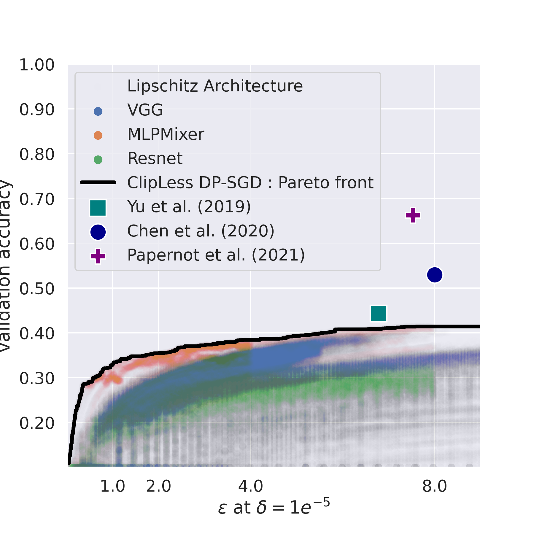
Figure 10: Accuracy/Privacy tradeoff on Cifar-10, split down per architecture used. While some architectures seems to perform better than others, we don’t advocate for the use of one over another. The results may not translate to all datasets, and may be highly dependant on the range chosen for hyper-parameters. While this figure provides valuable insights, identifying the best architecture is left for future works.

The sweeps have been done on various architectures such as Lipschitz VGGs, Lipschitz ResNets and Lipschitz MLP_Mixer. We can also break down the results per architecture, in figure 10. The MLP_Mixer architecture seems to yield the best results. This architecture is exactly GNP since the orthogonal linear transformations are applied on disjoint patches. To the contrary, VGG and Resnets are based on RKO convolutions which are not exactly GNP. Hence those preliminary results are compatible with our hypothesis that GNP layers should improve performance. Note that these results are expected to change as the architectures are further improved. It is also dependant of the range chosen for hyper-parameters. We do not advocate for the use of an architecture over another, and we believe many other innovations found in literature should be included before settling the question definitively.

D.2 Configuration of speed experiment

We detail below the environment version of each experiment, together with Cuda and cudnn versions. We rely on machine with 32GB RAM and a NVIDIA Quadro GTX 8000 graphic card with 48GB memory. The GPU uses driver version 495.29.05, cuda 11.5 (October 2021) and cudnn 8.2 (June 7, 2021). We use Python 3.8.

• For Jax, we used jax 0.3.17 (Aug 31, 2022) with jaxlib 0.3.15 (July 23, 2022), flax 0.6.0 (Aug 17, 2022) and optax 1.4.0 (Nov 21, 2022).

• For Tensorflow, we used tensorflow 2.12 (March 22, 2023) with tensorflow_privacy 0.7.3 (September 1, 2021).

• For Pytorch, we used Opacus 1.4.0 (March 24, 2023) with Pytorch (March 15, 2023).

• For lip-dp we used deel-lip 1.4.0 (January 10, 2023) on Tensorflow 2.8 (May 23, 2022).

For this benchmark, we used among the most recent packages on pypi. However the latest version of tensorflow privacy could not be forced with pip due to broken dependencies. This issue arise in clean environments such as the one available in google colaboratory.

D.3 Drop-in replacement with Lipschitz networks in vanilla DPSGD

Thanks to the gradient clipping of DP-SGD (see Algorithm 4), Lipschitz networks can be readily integrated in traditional DP-SGD algorithm with gradient clipping. The PGD algorithm is not mandatory: the back-propagation can be performed within the computation graph through iterations of Björck algorithm (used in RKO convolutions). This does not benefit from any particular speed-up over conventional networks - quite to the contrary there is an additional cost incurred by enforcing Lipschitz constraints in the graph. Some layers of deel-lip library have been recoded in Jax/Flax, and the experiment was run in Jax, since Tensorflow was too slow.

We use use the Total Amount of Noise (TAN) heuristic introduced in [64] to heuristically tune hyper-parameters jointly. This ensures fair covering of the Pareto front. Results are exposed in Figures 11(a) and 11(b).

Algorithm 4 Differentially Private Stochastic Gradient Descent : DP-SGD

Input: Neural network architecture $f(\cdot,\cdot)$
Input: Initial weights $\theta_{0}$, learning rate scheduling $\eta_{t}$, number of steps $N$, noise multiplier $\sigma$, L2 clipping value $C$ .

1:repeat

2:     for all $1\leq t\leq N-1$ do

3:         Sample a batch

$$\mathcal{B}_{t}={(x_{1},y_{1}),(x_{2},y_{2}),\ldots,(x_{b},y_{b})}.$$

4:         Create microbatches, compute and clip the per-sample gradient of cost function:

$$\tilde{g}_{t,i}\vcentcolon=\max(C,\nabla_{\theta_{t}}\mathcal{L}(\hat{y}_{i},y_{i})).$$

5:         Perturb each microbatch with carefully chosen noise distribution $b\sim\mathcal{N}(0,\sigma C)$ :

$$\hat{g}_{t,i}\leftarrow\tilde{g}_{t,i}+b_{i}.$$

6:         Perform projected gradient step:

$$\theta_{t+1}\leftarrow\Pi(\theta_{t}-\eta_{t}\hat{g}_{t,i}).$$

7:     end for

8:until privacy budget $(\epsilon,\delta)$ has been reached.

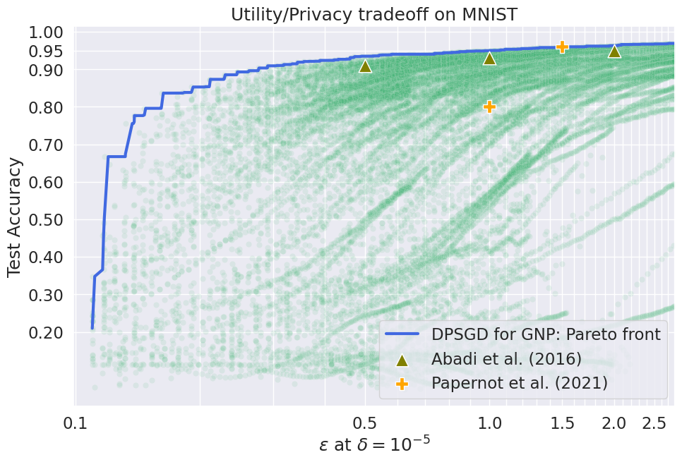
(a)

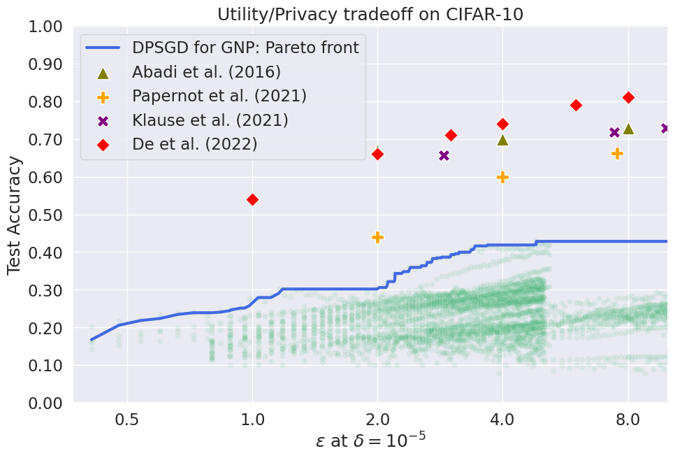
(b)

Figure 11: Privacy/utility trade-off for Gradient Norm Preserving networks trained under “vanilla” DP-SGD (with gradient clipping). Each green dot corresponds to a single epoch of one of the runs. Trajectories that end abruptly are due to the automatic early stopping of unpromising runs. Note that clipping + orthogonalization have a high runtime cost, which limits the number of epochs that reported.

D.4 Extended limitations

The main weakness of our approach is that it crucially rely on accurate computation of the sensitivity $\Delta$. This task faces many challenges in the context of differential privacy: floating point arithmetic is not associative, and summation order can a have dramatic consequences regarding numerical stability [55]. This is further amplified on the GPUs, where some operations are intrinsically non deterministic [56]. This well known issue is already present in vanilla DP-SGD algorithm. Our framework adds an additional point of failure: the upper bound of spectral Jacobian must be computed accurately. Hence Power Iteration must be run with sufficiently high number of iterations to ensure that the projection operator $\Pi$ works properly. The $(\epsilon,\delta)$-DP certificates only hold under the hypothesis that all computations are correct, as numerical errors can induce privacy leakages. Hence we check empirically the effective norm of the gradient in the training loop at the end of each epoch. No certificate violations were reported during ours experiments, which suggests that the numerical errors can be kept under control.

Appendix E Proofs of general results

This section contains the proofs of results that are either informally presented in the main paper, either formally defined in section A.2.

The informal Theorem 1 requires some tools that we introduce below.

Additionnal hypothesis for GNP networks. We introduce convenient assumptions for the purpose of obtaining tight bounds in Algorithm 2.

Assumption 1 (Bounded biases).

We assume there exists $B>0$ such that that for all biases $b_{d}$ we have $\|b_{d}\|\leq B$. Observe that the ball $\{\|b\|_{2}\leq B\}$ of radius $B$ is a convex set.

Assumption 2 (Zero preserving activation).

We assume that the activation fulfills $\sigma(\bf 0)=\bf 0$. When $\sigma$ is $S$-Lipschitz this implies $\|\sigma(x)\|\leq S\|x\|$ for all $x$. Examples of activations fulfilling this constraints are ReLU, Groupsort, GeLU, ELU, tanh. However it does not work with sigmoid or softplus.

We also propose the assumption 3 for convenience and exhaustivity.

Assumption 3 (Bounded activation).

We assume it exists $G>0$ such that for every $x\in\mathcal{X}$ and every $1\leq d\leq D+1$ we have:

$$\|h_{d}\|\leq G\quad\text{and}\quad\|z_{d}\|\leq G.$$ (27)

Note that this assumption is implied by requirement 2, assumption 1-2, as illustrated in proposition 3.

In practice assumption 3 can be fulfilled with the use of input clipping and bias clipping, bounded activation functions, or layer normalization. This assumption can be used as a “shortcut” in the proof of the main theorem, to avoid the “propagation of input bounds” step.

E.1 Main result

We rephrase in a rigorous manner the informal theorem of section 3.1. The proofs are given in section B. In order to simplify the notations, we use $X\vcentcolon=X_{0}$ in the following.

Proposition 3.

Norm of intermediate activations. Under requirement 2, assumptions 1-2 we have:

$$\|h_{t}\|\leq S\|z_{t}\|\leq\begin{cases*}(US)^{t}\left(X-\frac{SB}{1-SU}\right)+\frac{SB}{1-SU}&if $US\neq 1$,\\ SX+tSB&otherwise.\end{cases*}$$ (28)

In particular if there are no biases, i.e if $B=0$, then $\|h_{t}\|\leq S\|z_{t}\|\leq SX$ .

Proposition 3 can be used to replace assumption 3.

Proposition 4.

Lipschitz constant of dense Lipschitz networks with respect to parameters. Let $f(\cdot,\cdot)$ be a Lipschitz neural network. Under requirement 2, assumptions 1-2 we have for every $1\leq t\leq T+1$:

$$\|\frac{\partial f(\theta,x)}{\partial b_{t}}\|_{2} \leq(SU)^{T+1-t},$$ (29)

$$\|\frac{\partial f(\theta,x)}{\partial W_{t}}\|_{2} \leq(SU)^{T+1-t}\|h_{t-1}\|.$$ (30)

In particular, for every $x\in\mathcal{X}$, the function $\theta\mapsto f(\theta,x)$ is Lipschitz bounded.

Proposition 4 suggests that the scale of the activation $\|h_{t}\|$ must be kept under control for the gradient scales to distribute evenly along the computation graph. It can be easily extended to a general result on the per sample gradient of the loss, in theorem 1.

Theorem 1.

Bounded loss gradient for dense Lipschitz networks. Assume the predictions are given by a Lipschitz neural network $f$:

$$\hat{y}\vcentcolon=f(\theta,x).$$ (31)

Under requirements 1-2, assumptions 1-2, there exists a $K>0$ for all $(x,y,\theta)\in\mathcal{X}\times\mathcal{Y}\times\Theta$ the loss gradient is bounded:

$$\|\nabla_{\theta}\mathcal{L}(\hat{y},y)\|_{2}\leq K.$$ (32)

Let $\alpha=SU$ be the maximum spectral norm of the Jacobian between two consecutive layers.

If $\alpha=1$ then we have:

$$K=\mathcal{O}\left(LX+L\sqrt{T}+LSX\sqrt{T}+L\sqrt{BX}ST+LBST^{\nicefrac{{3}}{{2}}}\right).$$ (33)

The case $S=1$ is of particular interest since it covers most activation function (i.e ReLU, GroupSort):

$$K=\mathcal{O}\left(L\sqrt{T}+LX\sqrt{T}+L\sqrt{BX}T+LBT^{\nicefrac{{3}}{{2}}}\right).$$ (34)

Further simplification is possible if we assume $B=0$, i.e a network without biases:

$$K=\mathcal{O}\left(L\sqrt{T}(1+X)\right).$$ (35)

If $\alpha>1$ then we have:

$$\|\nabla_{\theta}\mathcal{L}(\hat{y},y)\|_{2} =\mathcal{O}\left(L\frac{\alpha^{T}}{\alpha-1}\left(\sqrt{T}(\alpha X+SB)+\frac{\alpha(SB+\alpha)}{\sqrt{\alpha^{2}-1}}\right)\right).$$ (36)

Once again $B=0$ (network with no bias) leads to useful simplifications:

$$\|\nabla_{\theta}\mathcal{L}(\hat{y},y)\|_{2} =\mathcal{O}\left(L\frac{\alpha^{T+1}}{\alpha-1}\left(\sqrt{T}X+\frac{\alpha}{\sqrt{\alpha^{2}-1}}\right)\right).$$ (37)

We notice that when $\alpha\gg 1$ there is an exploding gradient phenomenon where the upper bound become vacuous.

If $\alpha<1$ then we have:

$$\|\nabla_{\theta}\mathcal{L}(\hat{y},y)\|_{2} =\mathcal{O}\left(L\alpha^{T}\left(X\sqrt{T}+\frac{1}{(1-\alpha^{2})}\left(\sqrt{\frac{XSB}{\alpha^{T}}}+\frac{SB}{\sqrt{(1-\alpha)}}\right)\right)+\frac{L}{(1-\alpha)\sqrt{1-\alpha}}\right).$$ (38)

For network without biases we get:

$$\|\nabla_{\theta}\mathcal{L}(\hat{y},y)\|_{2} =\mathcal{O}\left(L\alpha^{T}X\sqrt{T}+\frac{L}{\sqrt{(1-\alpha)^{3}}}\right).$$ (39)

The case $\alpha\ll 1$ is a vanishing gradient phenomenon where $\|\nabla_{\theta}\mathcal{L}(\hat{y},y)\|_{2}$ is now independent of the depth $T$ and of the input scale $X$.

The informal theorem of section 3.1 is based on the aforementioned bounds, that have been simplified. Note that the definition of network differs slightly: in definition 3 the activations and the affines layers are considered independent and indexed differently, while the theoretical framework merge them into $z_{t}$ and $h_{t}$ respectively, sharing the same index $t$. This is without consequences once we realize that if $K=U=S$ and $2T=D$ then $(US)^{2}=\alpha^{2}=K^{2}$ leads to $\alpha^{2T}=K^{D}$. The leading constant factors based on $\alpha$ value have been replaced by $1$ since they do not affect the asymptotic behavior.

E.2 Proof of main result

Propositions 3 and 4 were introduced for clarity. They are a simple consequence of the Lemmas 1-3-4 used in the proof of Theorem 1. See the proof below for a complete exposition of the arguments.

See 1

Proof.

The control of gradient implicitly depend on the scale of the output of the network at every layer, hence it is crucial to control the norm of each activation.

Lemma 1 (Bounded activations).

If $US\neq 1$ for every $1\leq t\leq T+1$ we have:

$$\|z_{t}\|\leq U^{t}S^{t-1}\left(X-\frac{SB}{1-SU}\right)+\frac{B}{1-SU}.$$ (40)

If $US=1$ we have:

$$\|z_{t}\|\leq X+tB.$$ (41)

In every case we have $\|h_{t}\|\leq S\|z_{t}\|$.

Lemma proof..

From assumption 2, if we assume that $\sigma$ is $S$-Lipschitz, we have:

$$\|h_{t}\|=\|\sigma(z_{t})\|=\|\sigma(z_{t})-\sigma(\bf{0})\|\leq S\|z_{t}\|.$$ (42)

Now, observe that:

$$\|z_{t+1}\|=\|W_{t+1}h_{t}+b_{t+1}\|\leq\|W_{t+1}\|\|h_{t}\|+\|b_{t+1}\|\leq US\|z_{t}\|+B.$$ (43)

Let $u_{1}=UX+B$ and $u_{t+1}=SUu_{t}+B$ be a linear recurrence relation. The translated sequence $u_{t}-\frac{B}{1-SU}$ is a geometric progression of ratio $SU$, hence $u_{t}=(SU)^{t-1}(UX+B-\frac{B}{1-SU})+\frac{B}{1-SU}$. Finally we conclude that by construction $\|z_{t}\|\leq u_{t}$. ∎

The activation jacobians can be bounded by applying the chainrule. The recurrence relation obtained is the one automatically computed with back-propagation.

Lemma 2 (Bounded activation derivatives).

For every $T+1\geq s\geq t\geq 1$ we have:

$$\|\frac{\partial z_{s}}{\partial z_{t}}\|\leq(SU)^{s-t}.$$ (44)

Lemma proof..

The chain rule expands as:

$$\frac{\partial z_{s}}{\partial z_{t}}=\frac{\partial z_{s}}{\partial h_{s-1}}\frac{\partial h_{s-1}}{\partial z_{s-1}}\frac{\partial z_{s-1}}{\partial z_{t}}.$$ (45)

From Cauchy-Schwartz inequality we get:

$$\|\frac{\partial z_{s}}{\partial z_{t}}\|\leq\|\frac{\partial z_{s}}{\partial h_{s-1}}\|\cdot\|\frac{\partial h_{s-1}}{\partial z_{s-1}}\|\cdot\|\frac{\partial z_{s-1}}{\partial z_{t}}\|.$$ (46)

Since $\sigma$ is $S$-Lipschitz, and $\|W_{s}\|\leq U$, and by observing that $\|\frac{\partial z_{t}}{\partial z_{t}}\|=1$ we obtain by induction that:

$$\|\frac{\partial h_{s}}{\partial h_{t}}\|\leq(SU)^{s-t}.$$ (47)

∎

The derivatives of the biases are a textbook application of the chainrule.

Lemma 3 (Bounded bias derivatives).

For every $t$ we have:

$$\|\nabla_{b_{t}}\mathcal{L}(\hat{y},y)\|\leq L(SU)^{T+1-t}.$$ (48)

Lemma proof..

The chain rule yields:

$$\nabla_{b_{t}}\mathcal{L}(\hat{y},y)=(\nabla_{\hat{y}}\mathcal{L}(\hat{y},y))\frac{\partial z_{T+1}}{\partial z_{t}}\frac{\partial z_{t}}{\partial b_{t}}.$$ (49)

Hence we have:

$$\|\nabla_{b_{t}}\mathcal{L}(\hat{y},y)\|=\|\nabla_{\hat{y}}\mathcal{L}(\hat{y},y)\|\cdot\|\frac{\partial z_{T+1}}{\partial z_{t}}\|\cdot\|\frac{\partial z_{t}}{\partial b_{t}}\|.$$ (50)

We conclude with Lemma 2 that states $\|\frac{\partial z_{T+1}}{\partial z_{t}}\|\leq(US)^{T+1-t}$, with requirement 1 that states $\|\nabla_{\hat{y}}\mathcal{L}(\hat{y},y)\|\leq L$ and by observaing that $\|\frac{\partial z_{t}}{\partial b_{t}}\|=1$. ∎

We can now bound the derivative of the affine weights:

Lemma 4 (Bounded weight derivatives).

For every $T+1\geq t\geq 2$ we have:

$$\|\nabla_{W_{t}}\mathcal{L}(\hat{y},y)\| \leq L(SU)^{T}\left(X-\frac{SB}{1-SU}\right)+L(SU)^{T+1-t}\frac{SB}{1-SU}\text{ when }SU\neq 1,$$ (51)

$$\|\nabla_{W_{t}}\mathcal{L}(\hat{y},y)\| \leq LS\left(X+(t-1)B\right)\text{ when }SU=1.$$ (52)

In every case:

$$\|\nabla_{W_{1}}\mathcal{L}(\hat{y},y)\|\leq L(SU)^{T}X.$$ (54)

Lemma proof..

We proceed like in the proof of Lemma 3 and we get:

$$\|\nabla_{W_{t}}\mathcal{L}(\hat{y},y)\|\leq\|\nabla_{\hat{y}}\mathcal{L}(\hat{y},y)\|\cdot\|\frac{\partial z_{T+1}}{\partial z_{t}}\|\cdot\|\frac{\partial z_{t}}{\partial W_{t}}\|.$$ (55)

Which then yields:

$$\|\nabla_{W_{t}}\mathcal{L}(\hat{y},y)\|\leq L(SU)^{T+1-t}\cdot\|\frac{\partial z_{t}}{\partial W_{t}}\|.$$ (56)

Now, for $T+1\geq t\geq 1$, according to Lemma 1 we either have:

$$\|\frac{\partial z_{t}}{\partial W_{t}}\|\leq\|h_{t-1}\|\leq S\|z_{t-1}\|=(SU)^{t-1}\left(X-\frac{SB}{1-SU}\right)+\frac{SB}{1-SU},$$ (57)

or, when $US=1$:

$$\|\frac{\partial z_{t}}{\partial W_{t}}\| \leq\|h_{t-1}\|=S\|z_{t-1}\|=SX+(t-1)SB\text{ if }t\geq 2,$$ (58)

$$\|\frac{\partial z_{t}}{\partial W_{t}}\| \leq X\text{ otherwise}.$$ (59)

∎

Now, the derivatives of the loss with respect to each type of parameter (i.e $W_{t}$ or $b_{t}$) are know, and they can be combined to retrieve the overall gradient vector.

$$\theta=\{(W_{1},b_{1}),(W_{2},b_{2}),\ldots(W_{T+1},b_{T+1})\}.$$ (60)

We introduce $\alpha=SU$.

Case $\alpha=1$.

The resulting norm is given by the series:

$$\|\nabla_{\theta}\mathcal{L}(\hat{y},y)\|^{2}_{2} =\sum_{t=1}^{T+1}\|\nabla_{b_{t}}\mathcal{L}(\hat{y},y)\|^{2}_{2}+\|\nabla_{W_{t}}\mathcal{L}(\hat{y},y)\|^{2}_{2}$$ (61)

$$\leq L^{2}\left((1+X^{2})+\sum_{t=2}^{T+1}(1+(SX+(t-1)SB)^{2})\right)$$ (62)

$$\leq L^{2}\left(1+X^{2}+\sum_{u=1}^{T}(1+(SX+uSB)^{2})\right)$$ (63)

$$\leq L^{2}\left(1+X^{2}+\sum_{u=1}^{T}(1+S^{2}(X^{2}++2uBX+u^{2}B^{2}))\right)$$ (64)

$$\leq L^{2}\left(1+X^{2}+T(1+S^{2}X^{2})+S^{2}BXT(T+1)+S^{2}B^{2}\frac{T(T+1)(2T+1)}{6}\right).$$ (65)

Finally:

$$\|\nabla_{\theta}\mathcal{L}(\hat{y},y)\|_{2} =\mathcal{O}(L\sqrt{X^{2}+T+TS^{2}X^{2}+BS^{2}XT^{2}+B^{2}S^{2}T^{3}})$$ (66)

$$=\mathcal{O}\left(LX+L\sqrt{T}+LSX\sqrt{T}+L\sqrt{BX}ST+LBST^{\nicefrac{{3}}{{2}}}\right).$$ (67)

This upper bound depends (asymptotically) linearly of $L,X,S,B,T^{\nicefrac{{3}}{{2}}}$, when other factors are kept fixed to non zero value.

Case $\alpha\neq 1$.

We introduce $\beta=\frac{SB}{1-\alpha}$.

$$\|\nabla_{\theta}\mathcal{L}(\hat{y},y)\|^{2}_{2} =\sum_{t=1}^{T+1}\|\nabla_{b_{t}}\mathcal{L}(\hat{y},y)\|^{2}_{2}+\|\nabla_{W_{t}}\mathcal{L}(\hat{y},y)\|^{2}_{2}$$ (68)

$$\leq L^{2}\left(\alpha^{2T}\sum_{t=1}^{T+1}(((X-\beta)+\alpha^{1-t}\beta)^{2}+\alpha^{2-2t})\right)$$ (69)

$$\leq L^{2}\alpha^{2T}\left(\sum_{u=0}^{T}(((X-\beta)^{2}+2(X-\beta)\alpha^{-u}\beta+\alpha^{-2u}\beta^{2})+\alpha^{-2u})\right)$$ (70)

$$\leq L^{2}\alpha^{2T}\left((T+1)(X-\beta)^{2}+2(X-\beta)\beta\sum_{u=0}^{T}\alpha^{-u}+(\beta^{2}+1)\sum_{u=0}^{T}\alpha^{-2u}\right)$$ (71)

$$\leq L^{2}\alpha^{2T}\left((T+1)(X-\beta)^{2}+2(X-\beta)\beta\frac{\alpha-(\frac{1}{\alpha})^{T}}{\alpha-1}+(\beta^{2}+1)\frac{\alpha^{2}-(\frac{1}{\alpha^{2}})^{T}}{\alpha^{2}-1}\right).$$ (72)

Finally:

$$\|\nabla_{\theta}\mathcal{L}(\hat{y},y)\|_{2} \leq L\alpha^{T}\sqrt{(T+1)(X-\beta)^{2}+2(X-\beta)\beta\frac{\alpha-(\frac{1}{\alpha})^{T}}{\alpha-1}+(\beta^{2}+1)\frac{\alpha^{2}-(\frac{1}{\alpha^{2}})^{T}}{\alpha^{2}-1}}.$$ (73)

Now, the situation is a bit different for $\alpha<1$ and $\alpha>1$. One case corresponds to exploding gradient, and the other to vanishing gradient.

When $\alpha<1$ we necessarily have $\beta>0$, hence we obtain a crude upper-bound:

$$\|\nabla_{\theta}\mathcal{L}(\hat{y},y)\|_{2} =\mathcal{O}\left(L\alpha^{T}\left(X\sqrt{T}+\frac{1}{(1-\alpha^{2})}\left(\sqrt{\frac{XSB}{\alpha^{T}}}+\frac{SB}{\sqrt{(1-\alpha)}}\right)\right)+\frac{L}{(1-\alpha)\sqrt{1-\alpha}}\right).$$ (74)

Once again $B=0$ (network with no bias) leads to useful simplifications:

$$\|\nabla_{\theta}\mathcal{L}(\hat{y},y)\|_{2} =\mathcal{O}\left(L\alpha^{T}X\sqrt{T}+\frac{L}{\sqrt{(1-\alpha)^{3}}}\right).$$ (75)

This is a typical case of vanishing gradient since when $T\gg 1$ the upper bound does not depend on the input scale $X$ anymore.

Similarly, we can perform the analysis for $\alpha>1$, which implies $\beta<0$, yielding another bound:

$$\|\nabla_{\theta}\mathcal{L}(\hat{y},y)\|_{2} =\mathcal{O}\left(L\frac{\alpha^{T}}{\alpha-1}\left(\sqrt{T}(\alpha X+SB)+\frac{\alpha(SB+\alpha)}{\sqrt{\alpha^{2}-1}}\right)\right).$$ (76)

Without biases we get:

$$\|\nabla_{\theta}\mathcal{L}(\hat{y},y)\|_{2} =\mathcal{O}\left(L\frac{\alpha^{T+1}}{\alpha-1}\left(\sqrt{T}X+\frac{\alpha}{\sqrt{\alpha^{2}-1}}\right)\right).$$ (77)

We recognize an exploding gradient phenomenon due to the $\alpha^{T}$ term. ∎

E.3 Variance of the gradient

The result mentionned in section 3.1 is based on the following result, directly adapted from a classical result on concentration inequalities.

Corollary 2.

Concentration of stochastic gradient around its mean. Assume the samples $(x,y)$ are i.i.d and sampled from an arbitrary distribution $\mathcal{D}$. We introduce the R.V $g=\nabla_{\theta}\mathcal{L}(x,y)$ which is a function of the sample $(x,y)$, and its expectation $\bar{g}=\mathbb{E}_{(x,y)\sim\mathcal{D}}[\nabla_{\theta}\mathcal{L}(x,y)]$. Then for all $u\geq\frac{2}{\sqrt{b}}$ the following inequality hold:

$$\mathbb{P}(\|\frac{1}{b}\sum_{i=1}^{b}g_{i}-\bar{g}\|>uK)\leq\exp{\left(-\frac{\sqrt{b}}{8}(u-\frac{2}{\sqrt{b}})^{2}\right)}.$$ (78)

Proof.

The result is an immediate consequence of Example 6.3 p167 in [65]. We apply the theorem with the centered variable $X_{i}=\frac{1}{b}(g_{i}-\bar{g})$ that fulfills condition $\|X_{i}\|\leq\frac{c_{i}}{2}$ with $c_{i}=\frac{4K}{b}$ since $\|g_{i}\|\leq K$. Then for every $t\geq\frac{2K}{\sqrt{b}}$ we have:

$$\mathbb{P}(\|\frac{1}{b}\sum_{i=1}^{b}g_{i}-\bar{g}\|>t)\leq\exp{\left(-\frac{\sqrt{b}}{8K^{2}}(t-\frac{2K}{\sqrt{b}})^{2}\right)}.$$ (79)

We conclude with the change of variables $u=\frac{t}{K}$. ∎

References

- [1] Martin Abadi, Andy Chu, Ian Goodfellow, H Brendan McMahan, Ilya Mironov, Kunal Talwar, and Li Zhang. Deep learning with differential privacy. In Proceedings of the 2016 ACM SIGSAC conference on computer and communications security, pages 308–318, 2016.
- [2] Natalia Ponomareva, Hussein Hazimeh, Alex Kurakin, Zheng Xu, Carson Denison, H Brendan McMahan, Sergei Vassilvitskii, Steve Chien, and Abhradeep Thakurta. How to dp-fy ml: A practical guide to machine learning with differential privacy. arXiv preprint arXiv:2303.00654, 2023.
- [3] Cynthia Dwork, Frank McSherry, Kobbi Nissim, and Adam Smith. Calibrating noise to sensitivity in private data analysis. In Theory of Cryptography: Third Theory of Cryptography Conference, TCC 2006, New York, NY, USA, March 4-7, 2006. Proceedings 3, pages 265–284. Springer, 2006.
- [4] Mário S Alvim, Miguel E Andrés, Konstantinos Chatzikokolakis, Pierpaolo Degano, and Catuscia Palamidessi. Differential privacy: on the trade-off between utility and information leakage. In Formal Aspects of Security and Trust: 8th International Workshop, FAST 2011, Leuven, Belgium, September 12-14, 2011. Revised Selected Papers 8, pages 39–54. Springer, 2012.
- [5] Nicolas Papernot and Thomas Steinke. Hyperparameter tuning with renyi differential privacy. In International Conference on Learning Representations, 2022.
- [6] Jaewoo Lee and Daniel Kifer. Scaling up differentially private deep learning with fast per-example gradient clipping. Proceedings on Privacy Enhancing Technologies, 2021(1), 2021.
- [7] Xiangyi Chen, Steven Z Wu, and Mingyi Hong. Understanding gradient clipping in private sgd: A geometric perspective. Advances in Neural Information Processing Systems, 33:13773–13782, 2020.
- [8] Cem Anil, James Lucas, and Roger Grosse. Sorting out lipschitz function approximation. In International Conference on Machine Learning, pages 291–301. PMLR, 2019.
- [9] Cynthia Dwork, Aaron Roth, et al. The algorithmic foundations of differential privacy. Foundations and Trends® in Theoretical Computer Science, 9(3–4):211–407, 2014.
- [10] Leon Simon et al. Lectures on geometric measure theory. The Australian National University, Mathematical Sciences Institute, Centre …, 1983.
- [11] Christian Szegedy, Wojciech Zaremba, Ilya Sutskever, Joan Bruna, Dumitru Erhan, Ian Goodfellow, and Rob Fergus. Intriguing properties of neural networks. In International Conference on Learning Representations, 2014.
- [12] Yuichi Yoshida and Takeru Miyato. Spectral norm regularization for improving the generalizability of deep learning. arXiv preprint arXiv:1705.10941, 2017.
- [13] Peter L Bartlett, Dylan J Foster, and Matus Telgarsky. Spectrally-normalized margin bounds for neural networks. In Proceedings of the 31st International Conference on Neural Information Processing Systems, pages 6241–6250, 2017.
- [14] Ishaan Gulrajani, Faruk Ahmed, Martin Arjovsky, Vincent Dumoulin, and Aaron C Courville. Improved training of wasserstein gans. In Advances in Neural Information Processing Systems, volume 30, pages 5767–5777. Curran Associates, Inc., 2017.
- [15] Moustapha Cisse, Piotr Bojanowski, Edouard Grave, Yann Dauphin, and Nicolas Usunier. Parseval networks: Improving robustness to adversarial examples. In International Conference on Machine Learning, pages 854–863. PMLR, 2017.
- [16] Henry Gouk, Eibe Frank, Bernhard Pfahringer, and Michael J Cree. Regularisation of neural networks by enforcing lipschitz continuity. Machine Learning, 110:393–416, 2021.
- [17] Qiyang Li, Saminul Haque, Cem Anil, James Lucas, Roger B Grosse, and Jörn-Henrik Jacobsen. Preventing gradient attenuation in lipschitz constrained convolutional networks. In Advances in Neural Information Processing Systems (NeurIPS), volume 32, Cambridge, MA, 2019. MIT Press.
- [18] Louis Béthune, Thibaut Boissin, Mathieu Serrurier, Franck Mamalet, Corentin Friedrich, and Alberto Gonzalez Sanz. Pay attention to your loss : understanding misconceptions about lipschitz neural networks. In Alice H. Oh, Alekh Agarwal, Danielle Belgrave, and Kyunghyun Cho, editors, Advances in Neural Information Processing Systems, 2022.
- [19] Takeru Miyato, Toshiki Kataoka, Masanori Koyama, and Yuichi Yoshida. Spectral normalization for generative adversarial networks. arXiv preprint arXiv:1802.05957, 2018.
- [20] P-A Absil, Robert Mahony, and Rodolphe Sepulchre. Optimization algorithms on matrix manifolds. Princeton University Press, 2008.
- [21] Martin Arjovsky, Soumith Chintala, and Léon Bottou. Wasserstein generative adversarial networks. In International conference on machine learning, pages 214–223. PMLR, 2017.
- [22] Martín Abadi, Ashish Agarwal, Paul Barham, Eugene Brevdo, Zhifeng Chen, Craig Citro, Greg Corrado, Andy Davis, Jeffrey Dean, Matthieu Devin, Sanjay Ghemawat, Ian Goodfellow, Andrew Harp, Geoffrey Irving, Michael Isard, Yangqing Jia, Rafal Jozefowicz, Lukasz Kaiser, Manjunath Kudlur, Josh Levenberg, Dan Mane, Rajat Monga, Sherry Moore, Derek Murray, Chris Olah, Mike Schuster, Jonathon Shlens, Benoit Steiner, Ilya Sutskever, Kunal Talwar, Paul Tucker, Vincent Vanhoucke, Vijay Vasudevan, Fernanda Viegas, Oriol Vinyals, Pete Warden, Martin Wattenberg, Martin Wicke, Yuan Yu, and Xiaoqiang Zheng. Tensorflow: Large-scale machine learning on heterogeneous distributed systems, 2015.
- [23] Adam Paszke, Sam Gross, Francisco Massa, Adam Lerer, James Bradbury, Gregory Chanan, Trevor Killeen, Zeming Lin, Natalia Gimelshein, Luca Antiga, et al. Pytorch: An imperative style, high-performance deep learning library. Advances in neural information processing systems, 32, 2019.
- [24] Lloyd N Trefethen and David Bau. Numerical linear algebra, volume 181. Siam, 2022.
- [25] S Singla and S Feizi. Fantastic four: Differentiable bounds on singular values of convolution layers. In International Conference on Learning Representations (ICLR), 2021.
- [26] Airbus. Decomon. https://github.com/airbus/decomon, 2023.
- [27] Kaidi Xu, Zhouxing Shi, Huan Zhang, Yihan Wang, Kai-Wei Chang, Minlie Huang, Bhavya Kailkhura, Xue Lin, and Cho-Jui Hsieh. Automatic perturbation analysis for scalable certified robustness and beyond. Advances in Neural Information Processing Systems, 33:1129–1141, 2020.
- [28] Gagandeep Singh, Timon Gehr, Markus Püschel, and Martin Vechev. An abstract domain for certifying neural networks. Proceedings of the ACM on Programming Languages, 3(POPL):1–30, 2019.
- [29] Huan Zhang, Tsui-Wei Weng, Pin-Yu Chen, Cho-Jui Hsieh, and Luca Daniel. Efficient neural network robustness certification with general activation functions. Advances in neural information processing systems, 31, 2018.
- [30] H Brendan McMahan, Daniel Ramage, Kunal Talwar, and Li Zhang. Learning differentially private recurrent language models. In International Conference on Learning Representations, 2018.
- [31] Borja Balle, Gilles Barthe, and Marco Gaboardi. Privacy amplification by subsampling: Tight analyses via couplings and divergences. Advances in Neural Information Processing Systems, 31, 2018.
- [32] Yu-Xiang Wang, Borja Balle, and Shiva Prasad Kasiviswanathan. Subsampled rényi differential privacy and analytical moments accountant. In The 22nd International Conference on Artificial Intelligence and Statistics, pages 1226–1235. PMLR, 2019.
- [33] Yuqing Zhu and Yu-Xiang Wang. Possion subsampled rényi differential privacy. In International Conference on Machine Learning, pages 7634–7642. PMLR, 2019.
- [34] Yuqing Zhu and Yu-Xiang Wang. Improving sparse vector technique with renyi differential privacy. Advances in Neural Information Processing Systems, 33:20249–20258, 2020.
- [35] Ilya Mironov. Rényi differential privacy. In 2017 IEEE 30th computer security foundations symposium (CSF), pages 263–275. IEEE, 2017.
- [36] Ilya Mironov, Kunal Talwar, and Li Zhang. R’enyi differential privacy of the sampled gaussian mechanism. arXiv preprint arXiv:1908.10530, 2019.
- [37] Razvan Pascanu, Tomas Mikolov, and Yoshua Bengio. On the difficulty of training recurrent neural networks. In International conference on machine learning, pages 1310–1318. Pmlr, 2013.
- [38] Yoshua Bengio, Patrice Simard, and Paolo Frasconi. Learning long-term dependencies with gradient descent is difficult. IEEE transactions on neural networks, 5(2):157–166, 1994.
- [39] Ugo Tanielian and Gerard Biau. Approximating lipschitz continuous functions with groupsort neural networks. In International Conference on Artificial Intelligence and Statistics, pages 442–450. PMLR, 2021.
- [40] Zakaria Mhammedi, Andrew Hellicar, Ashfaqur Rahman, and James Bailey. Efficient orthogonal parametrisation of recurrent neural networks using householder reflections. In International Conference on Machine Learning, pages 2401–2409. PMLR, 2017.
- [41] Shuai Li, Kui Jia, Yuxin Wen, Tongliang Liu, and Dacheng Tao. Orthogonal deep neural networks. IEEE transactions on pattern analysis and machine intelligence, 43(4):1352–1368, 2019.
- [42] Asher Trockman and J Zico Kolter. Orthogonalizing convolutional layers with the cayley transform. In International Conference on Learning Representations, 2021.
- [43] Sahil Singla and Soheil Feizi. Skew orthogonal convolutions. In International Conference on Machine Learning, pages 9756–9766. PMLR, 2021.
- [44] El Mehdi Achour, François Malgouyres, and Franck Mamalet. Existence, stability and scalability of orthogonal convolutional neural networks. The Journal of Machine Learning Research, 23(1):15743–15798, 2022.
- [45] Sahil Singla and Soheil Feizi. Improved techniques for deterministic l2 robustness. arXiv preprint arXiv:2211.08453, 2022.
- [46] Xiaojun Xu, Linyi Li, and Bo Li. Lot: Layer-wise orthogonal training on improving l2 certified robustness. arXiv preprint arXiv:2210.11620, 2022.
- [47] Stephen P Boyd and Lieven Vandenberghe. Convex optimization. Cambridge university press, 2004.
- [48] Mathieu Serrurier, Franck Mamalet, Alberto González-Sanz, Thibaut Boissin, Jean-Michel Loubes, and Eustasio Del Barrio. Achieving robustness in classification using optimal transport with hinge regularization. In Proceedings of the IEEE/CVF Conference on Computer Vision and Pattern Recognition, pages 505–514, 2021.
- [49] Nicolas Papernot, Abhradeep Thakurta, Shuang Song, Steve Chien, and Úlfar Erlingsson. Tempered sigmoid activations for deep learning with differential privacy. In Proceedings of the AAAI Conference on Artificial Intelligence, volume 35, pages 9312–9321, 2021.
- [50] Florian Tramer and Dan Boneh. Differentially private learning needs better features (or much more data), 2021.
- [51] Soham De, Leonard Berrada, Jamie Hayes, Samuel L Smith, and Borja Balle. Unlocking high-accuracy differentially private image classification through scale. arXiv preprint arXiv:2204.13650, 2022.
- [52] Karen Simonyan and Andrew Zisserman. Very deep convolutional networks for large-scale image recognition. arXiv preprint arXiv:1409.1556, 2014.
- [53] Kaiming He, Xiangyu Zhang, Shaoqing Ren, and Jian Sun. Deep residual learning for image recognition. In Proceedings of the IEEE conference on computer vision and pattern recognition, pages 770–778, 2016.
- [54] Ilya O Tolstikhin, Neil Houlsby, Alexander Kolesnikov, Lucas Beyer, Xiaohua Zhai, Thomas Unterthiner, Jessica Yung, Andreas Steiner, Daniel Keysers, Jakob Uszkoreit, et al. Mlp-mixer: An all-mlp architecture for vision. Advances in neural information processing systems, 34:24261–24272, 2021.
- [55] David Goldberg. What every computer scientist should know about floating-point arithmetic. ACM computing surveys (CSUR), 23(1):5–48, 1991.
- [56] Hadi Jooybar, Wilson WL Fung, Mike O’Connor, Joseph Devietti, and Tor M Aamodt. Gpudet: a deterministic gpu architecture. In Proceedings of the eighteenth international conference on Architectural support for programming languages and operating systems, pages 1–12, 2013.
- [57] Mahyar Fazlyab, Alexander Robey, Hamed Hassani, Manfred Morari, and George Pappas. Efficient and accurate estimation of lipschitz constants for deep neural networks. Advances in Neural Information Processing Systems, 32, 2019.
- [58] Sébastien Bubeck et al. Convex optimization: Algorithms and complexity. Foundations and Trends® in Machine Learning, 8(3-4):231–357, 2015.
- [59] Olivier Bousquet and André Elisseeff. Stability and generalization. The Journal of Machine Learning Research, 2:499–526, 2002.
- [60] Colin McDiarmid et al. On the method of bounded differences. Surveys in combinatorics, 141(1):148–188, 1989.
- [61] Galen Andrew, Om Thakkar, Brendan McMahan, and Swaroop Ramaswamy. Differentially private learning with adaptive clipping. Advances in Neural Information Processing Systems, 34:17455–17466, 2021.
- [62] Jasper Snoek, Hugo Larochelle, and Ryan P Adams. Practical bayesian optimization of machine learning algorithms. Advances in neural information processing systems, 25, 2012.
- [63] Lisha Li, Kevin Jamieson, Giulia DeSalvo, Afshin Rostamizadeh, and Ameet Talwalkar. Hyperband: A novel bandit-based approach to hyperparameter optimization. The Journal of Machine Learning Research, 18(1):6765–6816, 2017.
- [64] Tom Sander, Pierre Stock, and Alexandre Sablayrolles. Tan without a burn: Scaling laws of dp-sgd. arXiv preprint arXiv:2210.03403, 2022.
- [65] Stéphane Boucheron, Gábor Lugosi, and Pascal Massart. Concentration inequalities: A nonasymptotic theory of independence. Oxford university press, 2013.