The ice composition close to the surface of comet 67P/Churyumov-Gerasimenko

Abstract

The relation between ice composition in the nucleus of comet 67P/Churyumov-Gerasimenko on the one hand and relative abundances of volatiles in the coma on the other hand is important for the interpretation of density measurements in the environment of the cometary nucleus. For the 2015 apparition, in situ measurements from the two ROSINA (Rosetta Orbiter Spectrometer for Ion and Neutral Analysis) sensors COPS (COmet Pressure Sensor) and DFMS (Double Focusing Mass Spectrometer) determined gas densities at the spacecraft position for the 14 gas species H₂O, CO₂, CO, H₂S, O₂, C₂H₆, CH₃OH, H₂CO, CH₄, NH₃, HCN, C₂H₅OH, OCS, and CS₂. We derive the spatial distribution of the gas emissions on the complex shape of the nucleus separately for 50 subintervals of the two-year mission time. The most active patches of gas emission are identified on the surface. We retrieve the relation between solar irradiation and observed emissions from these patches. The emission rates are compared to a minimal thermophysical model to infer the surface active fraction of H₂O and CO₂. We obtain characteristic differences in the ice composition close to the surface between the two hemispheres with a reduced abundance of CO₂ ice on the northern hemisphere (locations with positive latitude). We do not see significant differences for the ice composition on the two lobes of 67P/C-G.

Keywords: comets, 67P/Churyumov–Gerasimenko, ROSINA data, Rosetta mission, data analysis

1 Introduction

The formation process of comets in the solar nebula at large distances from the sun resulted in cometary nuclei consisting of a mixture of solid ices and non-volatile dust components, including a variety of organic compounds ^{1, 2}. The molecular inventory of the volatile species in the nucleus is reflected in the composition of the cometary coma, which can be observed from Earth and during spacecraft missions ³. The Rosetta mission ⁴ of the European Space Agency accompanied and investigated the Jupiter-family comet 67P/Churyumov-Gerasimenko (67P/C-G) during its 2015 apparition ⁵. Rosetta’s ROSINA instrument ⁶ (Rosetta Orbiter Spectrometer for Ion and Neutral Analysis) collected millions of in situ measurements in the coma. ROSINA consisted of three sensors, the COmet Pressure Sensor (COPS), the Double Focusing Mass Spectrometer (DFMS), and the Reflectron-type Time Of Flight (RTOF) mass spectrometer for the determination of neutral gas densities and of relative abundances. The observed gas species range from inorganic molecules ⁷, which include the most abundant volatiles H₂O, CO₂, and CO, to more complex organic molecules ⁸. Here, we focus our detailed, spatially resolved analysis on 14 volatiles which have been globally characterized in terms of gas production in Läuter et al. ⁹. The Rosetta mission additionally contained the remote sensing instruments MIRO ¹⁰ and VIRTIS ¹¹, which performed an independent analysis of the coma composition with respect to the ROSINA data.

The ROSINA data were obtained over a wide range of varying observational conditions. Coma measurements around the cometary nucleus began at a heliocentric distance of 3.6 au in August 2014, continued while approaching perihelion on August 13th 2015 at $1.24~{}\mathrm{au}$, and finally concluded after two years in September 2016 at a heliocentric distance of $3.7~{}\mathrm{au}$. The increasing solar irradiation toward perihelion is linked to a steep increase of gas and dust emissions. The operational orbit of the Rosetta spacecraft covered the surface of the rotating nucleus (rotation period about 12 hours) by a fast sampling (on the scale of hours) along the longitudinal coordinates and by a slower sampling (on the scale of days) along the latitudinal coordinates of the cometocentric system. The direct correlation of the spacecraft trajectory to peaks in density yields a localization of gas emissions on the surface ¹². High resolution OSIRIS images ^{13, 14, 15} of comet 67P/C-G revealed the complicated non-convex shape of the nucleus with a volume of $\approx 19~{}\mathrm{km}^{3}$, which requires moving beyond spherical approximations of the nucleus geometry. The spacecraft distance to the nucleus ranged from a few kilometers to more than $1000\,\mathrm{km}$ which affects the spatial resolution of the instruments on the spacecraft. The Rosetta mission provided the unique opportunity to monitor the evolution of the cometary coma with in situ measurements over two years. Cometary flyby missions collect in situ data as well, but are limited to much shorter time periods ^{16, 5}. The number of comets accessible via Earth bound observations is more comprehensive and covers, besides comets in the solar system, ^{17, 18, 19} also interstellar objects ^{20, 21}.

One goal of the observations is to determine the composition of the cometary material ²². We derive maps of best-fit emission rates on the cometary surface which reproduce the measured density variations at the spacecraft position within the inner coma. The emission maps are obtained by adjusting the emission rates placed on a complex shape of the nucleus within a forward/inverse modeling approach. This approach was introduced in Kramer et al. ²³ and Läuter et al. ^{24, 9}, it is briefly reviewed in Section 2, and it does away with the assumption of a spherical symmetric gas expansion of Haser-type models ²⁵. Kramer et al. ²³ retrieved surface maps showing the emission rates of neutral gas for three different time intervals and found a strong correlation between enhanced gas activity months before perihelion and locations of dust outbursts imaged around perihelion ²⁶. Läuter et al. ²⁴ extended this analysis to the major species H₂O, CO₂, CO and O₂ and to the entire duration of the Rosetta mission of two years. The data set was later enlarged to determine the temporal changes of the global production rate of 14 species analyzed by ROSINA ⁹.

Here, we construct and analyze the surface emission rate of the 14 species. In Sections 3 and 5 we compare our results with independent observations, which directly image the surface using optical and spectroscopic measurements ^{16, 27}. The detection and analysis of small surface areas based on OSIRIS images has been limited to specific regions and observation windows ¹⁶. An automated approach to map surface deformations and changes seen by optical instruments across the entire nucleus will improve this comparative approach in the future ²⁸.

Section 4 introduces a minimal thermophysical model. The nucleus material close to the surface consists of a mixture of various icy components available for sublimation processes and non-volatile dust grains, partly lifted up by the stream of gas. The modeling of the energy and mass fluxes within the nucleus requires a thermophysical model to relate the ice composition to the localized gas emission ^{29, 30, 31, 32, 33, 34, 35}. One class of thermophysical models considers the sublimation in response to the irradiation via a steady-state process (the models are discussed e.g. in Keller et al. ³⁶). This allows correlating the sublimation rate with solar irradiation and determining the fraction of the surface that is active. The assumption of a completely homogeneous ice distribution in these models does not explain the observed non-gravitational accelerations ^{37, 38, 39} and changes of the rotational state of the nucleus ⁴⁰, in particular the small changes of the orientation of the rotation axis⁴¹. In Section 5 we discuss the relation between the surface production and the composition of the near-surface ices.

2 Data and gas model in the coma

The data processing and analysis of the measured coma densities and abundances follows our forward/inverse model approach described in previous papers ^{23, 24, 9} and is reviewed briefly in this Section. The starting point is the combination of two data sets, one from the COPS sensor, the other one from the DFMS sensor of the ROSINA instrument.

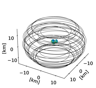
Figure 1: Spacecraft trajectory around comet 67P/C-G between 10 km to 20 km for subinterval $I_{4}$, 317 days to 302 days before perihelion.

DFMS collected the relative abundances of the gas species $s=$ H₂O, CO₂, CO, H₂S, O₂, C₂H₆, CH₃OH, H₂CO, CH₄, NH₃, HCN, C₂H₅OH, OCS, and CS₂ at numerous spacecraft positions within the coma of 67P/C-G. In combination with the absolute density of the neutral gas (from COPS), the relative abundances for each gas species yield the absolute densities of these species ^{7, 42}. In the following, we consider measurements between August 1st 2014 and September 5th 2016. This period spans 377 days before the perihelion passage to 390 days afterwards. We subdivide this interval for the analysis into 50 separated time subintervals $I_{1}$, …, $I_{50}$, varying in duration between 7 days and 29 days. The duration of the subintervals is taken as short as possible to satisfy the model assumption of constant solar irradiation conditions with respect to the heliocentric distance $r_{\mathrm{h}}$ within one subinterval. The minimal duration of any subinterval is dictated by two conditions. First, the sub-spacecraft position should have overflown almost the complete surface area of the nucleus. This condition is met for example, as shown in Figure 1, for the spacecraft trajectory within the subinterval $I_{4}$ around 310 days before perihelion. Rosetta’s orbit varied considerably over the mission and for the used data set the spacecraft distance to the nucleus changed from 8 km to $\approx{}500~{}\mathrm{km}$. The second condition is that we require at least as many gas density measurements as there are undetermined surface emitters (3996 in our model). The number of available measurements differs across subintervals and species and varies from 4443 points for CO to 19212 points for H₂O ⁹. For a small number of subintervals, some species are excluded from the analysis due to missing data points. For the species $s$ in the subinterval $I_{j}$ we denote the set of data points by $D_{s,j}=\{(t_{\mathrm{data}},\rho_{\mathrm{data}})\}$, the measurement times by $t_{\mathrm{data}}\in I_{j}$ and the measured density by $\rho_{\mathrm{data}}$ at the spacecraft position $\vec{x}_{\mathrm{sc}}(t_{\mathrm{data}})$. To reduce noise effects, our definition of $D_{s,j}$ excludes some outlying data points selected by a $2\sigma$ criterion described in Läuter et al. ⁹.

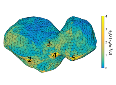
Figure 2: Shape of the 67P/C-G nucleus with 3996 triangular elements. The colors represent surface emission rates for H₂O (averaged from 50 days before to 50 days after perihelion), the numbers refer to surface patches.

For each gas species $s$ within the subinterval $I_{j}$ we construct a forward coma model. The model considers a steady-state flow of collisionless neutral gas into the vacuum domain around the nucleus up to a distance of $\approx{}500\,\mathrm{km}$ ²³. The coma model makes several assumptions to reduce the number of open parameters and to facilitate the processing and assimilation of the complete ROSINA data set. For instance, we neglect collisions and changes of the gas velocity, because most of the time the spacecraft trajectory was outside the region of gas acceleration. These effects could be incorporated by solving the gas equations for rarefied gas based on the direct simulation Monte Carlo method ⁴³, which has been applied to comet 67P/C-G ^{44, 45}. However, the increased computational effort limits the possible spatial resolution required for the determination of gas sources on the surface ^{46, 47}. A fixed number of equally spaced gas sources on the cometary surface serve as emitters for the gas flow in space. The shape of the nucleus is approximated by a surface mesh with $N_{\mathrm{E}}=3996$ triangular elements $E_{i}$. The shape in Figure 2 is derived from the high resolution shape of Preusker et al. ¹⁵ and features an average size, taken as the diameter of a circle with the same area, of 120 m for the triangular elements $E_{i}$. Each element $E_{i}$ contains one gas source with the surface emission rate $\dot{\rho}_{s,i,j}$ (see Eq. (4) in Kramer et al. ²³) which represents the time averaged gas production in the subinterval $I_{j}$. Narasimha ⁴⁸ provides an expression for the gas cloud originating from a single gas source with the density $\rho_{i}(\dot{\rho}_{s,i,j},\vec{x}_{\mathrm{sc}})$ at the spacecraft position $\vec{x}_{\mathrm{sc}}$. $\rho_{i}$ contains two adjustable parameters, the gas velocity $u_{0}$ into the vertical outflow direction and the cone parameter $U_{0}=3$ for the density distribution. Here, we take $u_{0}$ to be the function of $r_{\mathrm{h}}$ given by Hansen et al. ⁴⁴ and assume the same value of $u_{0}$ for all gas species ¹⁰. Recapitulating equation (5) in Kramer et al. ²³, the steady-state gas density at the spacecraft position

$$\rho_{s,j}(\vec{x}_{\mathrm{sc}})=\sum_{i=1}^{N_{\mathrm{E}}}\mathrm{occ}_{i}(\vec{x}_{\mathrm{sc}})\rho_{i}(\dot{\rho}_{s,i,j},\vec{x}_{\mathrm{sc}})$$ (1)

is the superposition of element-wise contributions with the occlusion function $\mathrm{occ}_{i}(\vec{x}_{\mathrm{sc}})$. For each subinterval $I_{j}$ we seek the surface emission rates $\dot{\rho}_{s,i,j}$ giving best agreement between model densities and observed coma densities $\rho_{s,i}(\vec{x}_{\mathrm{sc}}(t_{\mathrm{data}}))=\rho_{\mathrm{data}}$ for all data points $(t_{\mathrm{data}},\rho_{\mathrm{data}})\in D_{s,j}$. This requires us to solve the least-squares optimization problem given by equation (7) of Kramer et al. ²³. We refer to this step as applying the inverse model.

3 Gas emission rates and spatial distribution

name	time interval	$r_{\mathrm{h}}~{}[\mathrm{au}]$	sub solar lat.
perihelion	August 13th 2015	1.24	$-52^{\circ}$
$I_{\mathrm{inbound}}$	330 to 270 days before perihelion	3.0 – 3.4	$+37^{\circ}$ – $+42^{\circ}$
$I_{\mathrm{ph}}$	50 before to 50 days after perihelion	1.24 – 1.4	$-52^{\circ}$ – $-18^{\circ}$
$I_{\mathrm{outbound}}$	340 to 390 days after perihelion	3.4 – 3.7	$+14^{\circ}$ – $+19^{\circ}$

Table 1: Definition of time intervals considered in the analysis of the 2015 apparition of comet 67P/C-G.

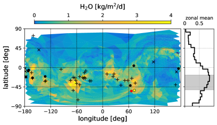
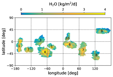
Figure 3: Surface emission rates for H₂O, averaged from 50 days before to 50 days after perihelion (see $I_{\mathrm{ph}}$ in Table 1), cometocentric Cheops coordinate system ⁴⁹. Left panel: surface map and corresponding zonal mean. $+$ markers ²⁶ denote outburst locations; $\times$ markers ⁵⁰, black dots ⁵¹, and yellow dot ⁵² denote water-ice patches; red dot ⁵³ denotes a CO₂-ice patch. The gray bar denotes the range of subsolar latitudes within $I_{\mathrm{ph}}$. Right panel: definition of the patches $A_{1}$, …, $A_{10}$ with the highest emission rates (dominated by H₂O near perihelion).

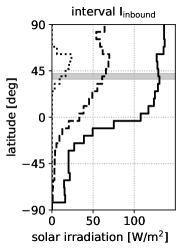
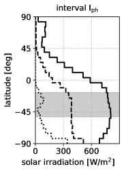
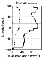
Figure 4: Solar irradiation onto the surface of 67P/C-G, diurnal average and zonal mean. The gray bar denotes the range of subsolar latitudes during the time interval. Left panel: time interval $I_{\mathrm{inbound}}$ (see Table 1), mid panel: time interval $I_{\mathrm{ph}}$, right panel: time interval $I_{\mathrm{outbound}}$. Dotted line: minimum irradiation, dashed line: mean irradiation, continuous line: maximum irradiation.

The inverse model determines the surface emission rates, which can be spatially integrated to obtain the global production rates $Q_{s}$ ⁹. The production rates increase toward perihelion, peak at 16 to 27 days after perihelion, and decrease as the solar irradiation diminishes for larger heliocentric distances ^{44, 54, 55}. Within the previous papers ^{24, 9} we have described the temporal evolution of the production rates as well as the surface localization of sources for the major species H₂O, CO₂, CO, and O₂. The production rates around perihelion (within the time interval $I_{\mathrm{ph}}$, see Table 1) represent the major part of the global gas production within a complete apparition. Analyzing the long term trend of the production rate 190 days after perihelion by a power law fit, we distinguished two groups of species. The CO₂ group features a slower production decay with decreasing solar irradiation (with exponents $-3\leq\alpha$), while the H₂O group displays a faster production decay with exponents exceeding $\alpha\leq-4.5$ ^{56, 9}.

The surface emission rates $\dot{\rho}_{\mathrm{H}_{2}\mathrm{O}}$ across the entire surface are represented as a surface map in Figures 2 and 3 for the predominant gas species water on 67P/C-G in the interval $I_{\mathrm{ph}}$. To relate these emission rates to solar irradiation qualitatively, the middle panel in Figure 4 shows the zonal mean of the incoming solar irradiation during this time interval. The southern hemisphere receives the largest part of the solar irradiation at subsolar latitudes between $-52^{\circ}$ and $-18^{\circ}$ within the interval $I_{\mathrm{ph}}$. We define the hemispheres as being separated by the equatorial plane through the center of the nucleus. Thus the southern and northern hemispheres ($A_{\mathrm{SH}}$ and $A_{\mathrm{NH}}$) are the surface locations with negative and positive latitudes in the cometocentric Cheops coordinate system ⁴⁹, respectively. The zonal mean of the water production and the irradiation are strongly correlated. Both, water production and maximum solar irradiation peak around latitudes between $-25^{\circ}$ and $-50^{\circ}$. Outside the perihelion period, the relation between sub solar latitude and the latitudes of dominant emission is more involved. For instance active CO₂ and CO regions continue to emit in the south 300 days after perihelion ²³, while the H₂O emission regions shift to the North along with the sub solar latitude ²⁴.

region	center (long,lat)	description
$A_{\mathrm{SH}}$		southern hemisphere
$A_{\mathrm{NH}}$		northern hemisphere
$A_{\mathrm{SL}}$		small lobe
$A_{\mathrm{BL}}$		big lobe
$A_{1}$	$(-165^{\circ},-15^{\circ})$	Imhotep, Apis, Khonsu, $A_{\mathrm{BL}}$
$A_{2}$	$(-130^{\circ},-30^{\circ})$	Khonsu, Atum, $A_{\mathrm{BL}}$
$A_{3}$	$(-85^{\circ},5^{\circ})$	Anuket, Hapi
$A_{4}$	$(-70^{\circ},-40^{\circ})$	Anuket, Sobek
$A_{5}$	$(-45^{\circ},-20^{\circ})$	Wosret, $A_{\mathrm{SL}}$
$A_{6}$	$(25^{\circ},-10^{\circ})$	Bastet, Wosret, $A_{\mathrm{SL}}$
$A_{7}$	$(75^{\circ},-30^{\circ})$	Anhur, Bes, Khepry, $A_{\mathrm{BL}}$
$A_{8}$	$(125^{\circ},-50^{\circ})$	Bes, Imhotep, $A_{\mathrm{BL}}$
$A_{9}$	$(145^{\circ},40^{\circ})$	Ash, $A_{\mathrm{BL}}$
$A_{10}$	$(15^{\circ},15^{\circ})$	Maat, Bastet, $A_{\mathrm{SL}}$

Table 2: Surface patches and their coordinates of the center, placement with respect to the lobes and to geomorphological features ⁵⁷ on 67P/C-G.

The water emission map shown in Figure 3, left panel, allows us to identify the most active patches²⁴ $A_{1}$–$A_{10}$, highlighted in the right panel of Figure 3. These patches overlap partly with the geomorphological features defined by El-Maarry et al. ⁵⁷. The patches are located on the southern and northern hemispheres $A_{\mathrm{SH}}$, $A_{\mathrm{NH}}$, and on the two lobes $A_{\mathrm{SL}}$, and $A_{\mathrm{BL}}$, see Table 2. The patches $A_{2}$–$A_{5}$ are marked on the three-dimensional shape model in Figure 2. Although the area of all 10 patches covers only 1/5 of the entire surface area, their combined water emission represents almost half of the global water emission.

The local emission depends on two independent properties of a patch, the composition of the nucleus material and the solar irradiation condition which will be further discussed in Section 4. To discuss the localization of the gas emissions, for a patch $A_{p}$ we define the mean production by the average value of the surface emission rate over the patch $A_{p}$. At perihelion for water, mean production varies between $0.7\,\mathrm{kg}/\mathrm{m}^{2}/\mathrm{d}$ on patch $A_{3}$ and $3.4\,\mathrm{kg}/\mathrm{m}^{2}/\mathrm{d}$ on the most active patch $A_{4}$. To quantify just the activity of a patch $A_{p}$, we introduce the activity ratio $a_{p}$ as the mean production divided by the global production rate per area $Q_{s}/|A_{\mathrm{67P}}|$. $Q_{s}/|A_{\mathrm{67P}}|$ is evaluated based on $Q_{s}$ in Table 2 of Läuter et al.⁹ and the entire surface area $A_{\mathrm{67P}}=44.31\times 10^{6}\,\mathrm{m}^{2}$ of 67P/C-G which yields the value $1.1\,\mathrm{kg}/\mathrm{m}^{2}/\mathrm{d}$ for water. Around perihelion this implies activity ratios for the patches $A_{3}$ and $A_{4}$ of $a_{3}=0.7$ and $a_{4}=3.2$, respectively. The surface $A_{\mathrm{67P}}$ is related to our smoothed shape model in Section 2 and thus it is smaller compared to reported areas ^{40, 15} for high-resolution shape models which vary between $[46.9\pm 2.5]\times 10^{6}\,\mathrm{m}^{2}$ and $[51.7\pm 0.1]\times 10^{6}\,\mathrm{m}^{2}$. This effects the production rates in the order of 10% and can be taken into account by rescaling the surface emissions reported here accordingly.

In the Refs. ^{23, 24} we show the high correlation of the most active gas emitting patches to short-lived outbursts ²⁶ ($+$ markers in Figure 3). In particular the activity on the patches $A_{4}$, $A_{5}$ (regions Sobek and Wosret) displays a strong correlation with the outbursts. Morphological changes indicating gas activity in $A_{5}$ have been reported ^{58, 59} around perihelion and later during the outbound Rosetta mission phase. For the duration of two years, Oklay et al. ⁵⁰ repeatedly observed water-ice-rich areas close to patch $A_{1}$ up to a size of $15000~{}\mathrm{m}^{2}$ ($\times$ markers in Figure 3). In the time around 300 days before and around perihelion, Barucci et al. ⁵¹ find 8 icy patches (black dots in Figure 3) consisting of water ice. Six of these icy patches are located close to patches $A_{1}$ (Imhotep), $A_{2}$ (Khonsu, Atum), and $A_{7}$ (Anhur). One hundred days before perihelion Fornasier et al. ⁵² reported two $1500~{}\mathrm{m}^{2}$ areas in the Anhur-Bes region with H₂O (yellow dot in Figure 3) and CO₂ (red dot in Figure 3) reservoirs ⁵³. Both are located in patch $A_{7}$.

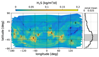
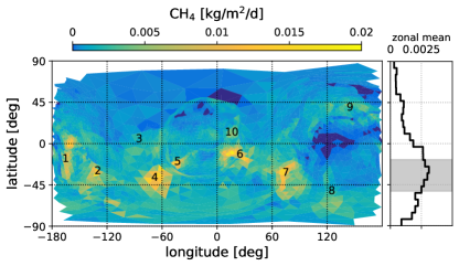
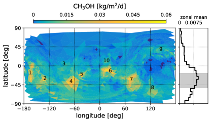
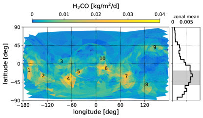
Figure 5: Surface emission rates for the minor gas species H₂S, CH₄, CH₃OH, and H₂CO, averaged from 50 days before perihelion to 50 days after perihelion (see $I_{\mathrm{ph}}$ in Table 1).

In addition to an increased emission rate for water, the patches $A_{1}$–$A_{10}$ also correspond to regions of enhanced emission rate for the major species CO, and O₂ around perihelion in the interval $I_{\mathrm{ph}}$ ⁹. For CO₂, the enhanced patches are restricted to the southern hemisphere. Around perihelion, Figure 5 shows the spatial distribution of the emission rate for (H₂S, CH₄) in the CO₂ group and for (CH₃OH, H₂CO) in the H₂O group. For these gases, peak production rates ⁹ range from $4.4\times 10^{26}~{}\mathrm{molecules}/\mathrm{s}$ for H₂S down to $8.2\times 10^{25}~{}\mathrm{molecules}/\mathrm{s}$ for CH₄. Similar to the major species, the minor species display their peak emission rate in all southern patches $A_{1}$, $A_{2}$, $A_{4}$–$A_{8}$. The activity ratio $a_{p}$ varies between 1.1 for CH₄ on patch $A_{8}$ and 3.2 for CH₃OH on $A_{4}$, as well as for CH₄ on $A_{6}$. The activity within the most active patches A₄ and A₆ in the South and the peak of the zonally averaged emission rate in the southern mid latitudes correlates closely with the solar irradiation shown in Figure 4, middle panel.

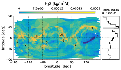
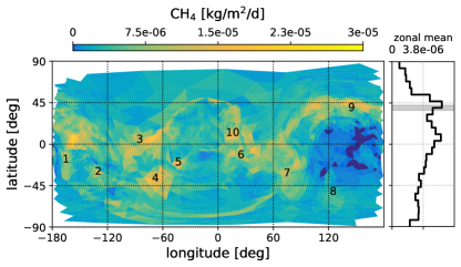
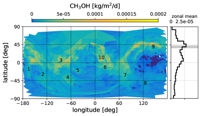
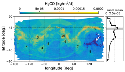
Figure 6: Surface emission rates for the minor gas species H₂S, CH₄, CH₃OH, and H₂CO, averaged from 330 days to 270 days before perihelion (see $I_{\mathrm{inbound}}$ in Table 1).

Next we discuss the distribution of surface emission rates approximately 300 days before perihelion (interval $I_{\mathrm{inbound}}$ in Table 1), shown in Figure 6. The peaks of the zonal mean emission rate for the minor gases H₂S, CH₄, CH₃OH and H₂CO are located close to northern subsolar latitudes between $+37^{\circ}$ and $+42^{\circ}$. The bi-lobed shape of the nucleus, see Figure 2, leads to zonally averaged irradiation conditions with significant illumination of the entire northern hemisphere and also partially of the southern hemisphere, see the left panel of Figure 4. This zonal mean of the irradiation closely correlates with the zonal mean of the emission rate across both hemispheres, see Figure 6. For all four species we find increased activity ratios ($a_{p}>1.7$) on the northern patches $A_{3}$, $A_{9}$, and $A_{10}$. The gases of the H₂O group show no significant active areas on the southern hemisphere, similar to H₂O and O₂ at that time ²⁴. In contrast, CO₂ already displays active areas in the South ²⁴, although the solar irradiation does not peak at these latitudes. This property is also shared by the other gases H₂S and CH₄ in the CO₂ group. For both gases and CO₂ the activity ratios on the southern patches $A_{1}$, $A_{4}$, and $A_{6}$ are at least 1.3. These three patches already show a presence of gas sources 300 days before perihelion, long before these areas become the most active emitters of the minor and major species.

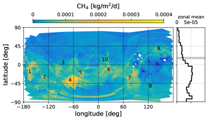
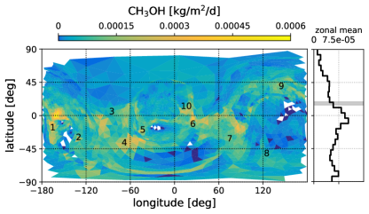
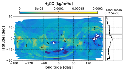
Figure 7: Surface emission rates for the minor gas species H₂S, CH₄, CH₃OH, and H₂CO, averaged from 340 days to 390 days after perihelion (see $I_{\mathrm{outbound}}$ in Table 1).

For the outbound time interval $I_{\mathrm{outbound}}$ (see Table 1) the discussion is complemented by the spatial distribution of emission rates in Figure 7 for the minor species H₂S, CH₄, CH₃OH and H₂CO. 300 days after perihelion, when the solar irradiation is diminished by more than a factor of 5 (see the right panel of Figure 4). The two northern patches $A_{3}$ and $A_{9}$ do not produce significantly more CO₂, H₂S and CH₄ than the mean with activity ratios between 1.0 and 1.2. In the southern patches A₁, A₄, and A₆ at least twice as much of these three species is emitted with activity ratios between 2.2 and 5.5. These areas with high emission rates during outbound time have already been reported ²⁴ for CO₂, O₂, and CO. For the species C₂H₆, NH₃, HCN, C₂H₅OH, OCS, and CS₂, the spatial distribution of emission rates is shown in the Figures of the Appendix.

4 Sublimation and solar irradiation

Solar irradiation provides the main energy influx to the icy components close to the cometary surface and drives the gas sublimation into the surrounding space. In the last Section we examined the general correlation between localized emission rates on the surface and seasonal irradiation. A quantitative analysis of this relation is the foundation for any thermophysical modeling ^{5, 30}. Thermophysical models predict the gas sublimation by evaluating all energy fluxes like incoming and outgoing radiation, heat conduction within the cometary material, and the energy going into the sublimation phase changes. Thermal inertia due to energy exchange with subsurface layers results in retardation effects on the diurnal and seasonal scale. This leads to a partial decoupling of instantaneous irradiation and gas release. In addition the presence of different volatiles, possibly refractory material and dust cover needs to be taken into account ^{60, 61, 62, 63}.

Another consideration is the trapping and sealing off of ices consisting of different volatiles. Amorphous water ice is able to trap minor species (like CO₂) and therefore it can affect the availability of volatile reservoirs at the sublimation front of water in the material column ⁶⁴. Trapped species escape at higher temperature compared to their specific sublimation temperature ^{29, 27}. For comet 67P/C-G, we find that the temporal evolution of the minor gas species over the 2015 apparition suggests a grouping of minor species into those following CO₂ and H₂O, as defined in Section 3. The linked temporal evolution of the production rates of a respective minor species with a H₂O or CO₂ major species might indicate a trapping of the minor volatile ⁵⁶.

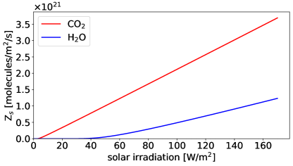
Figure 8: Sublimation rate for H₂O and CO₂ and for irradiation conditions on comet 67P/C-G based on the simplified sublimation model in Eq. (2).

The microscopic thermophysical models for cometary material composed of different ices and dust requires additional parameters, many of which are unknown or uncertain ⁶⁵. Therefore, we work in the following with a reduced parameters approach in a minimal thermophysical model for describing the sublimation of H₂O and CO₂ in response to the incoming radiation. We consider each facet (average diameter 120 m) as representing a separate vertical column consisting of a porous mixture of ices together with dust. We do not take amorphous water into account and assume that H₂O and CO₂ sublimate independently, and possibly at different depths. The non-trapping and non-blocking assumption between H₂O and CO₂ is commonly applied in thermophysical models, see for instance ⁶⁴. The independence of the H₂O and CO₂ sublimation leads to the coexistence of two vertically stacked sublimation fronts ⁶⁵ at two distinct temperatures, with H₂O sublimating closer to the surface and with the CO₂ sublimation front at a larger depth (about 1.9 m according to Davidsson et al. ⁶⁵). The depth values of the sublimation front are seen as averaged values adjusted to match the observed CO₂ release. To reduce the complexity we map the complex structure of the vertical columns into a direct relation between incoming irradiation and the gas production of a surface partially consisting of ice. This approach allows one to determine the effective fraction of a fictitious icy surface which reproduces the observed emission rates ^{36, 41}. The effective surface fraction $f_{p}$ is determined independently for H₂O and CO₂ and with respect to a completely covered body by the respective ice species ($f_{p}=1$). The sublimation rate at $f_{p}=1$ for both gas species $s=$ H₂O and CO₂ is determined from the energy balance between the solar irradiation $I$, the re-emitted radiation, and the sublimation rate $Z_{s}(T_{s})$ together with the latent heat of sublimation ($L_{s}$)

$$(1-A)I=\epsilon\sigma T_{s}^{4}+Z_{s}(T_{s})L_{s}.$$ (2)

This relation provides a non-linear constraint for the temperature $T_{s}$. Here we assume ³⁶ a bolometric Bond albedo of $A=0.01$, $\epsilon=0.9$ for the emissivity, and $\sigma$ denotes the Stefan-Boltzmann constant. Different values for the bond albedo between $0.01$ and $0.04$ have been considered in the literature ^{36, 66, 64}, which do not change our analysis appreciably. The latent heat of sublimation $L_{s}$ and Hertz-Knudsen relation $Z_{s}(T_{s})=2p_{s}(T_{s})/\pi/v_{s}(T_{s})$ are specific for the gas species $s$ with the vapor pressure $p_{s}(T_{s})$, the thermal velocity $v_{s}(T_{s})=\sqrt{8RT_{s}/\pi/\mu_{s}}$, the molar mass $\mu_{s}$, and the gas constant $R$. With this model approach one obtains the temperature $T_{s}$ and the corresponding sublimation rate $Z_{s}(I)$ for any given irradiation $I$, see Figure 8. The temperature $T_{s}$ depends on the species and the gas emission is not affected by the occurrence of the other species. We discuss the sublimation rates for the two major species H₂O and CO₂ based on the volatile properties tabulated by Huebner et al. ³⁰. For water we assume a temperature independent heat of sublimation $L_{\mathrm{H}_{2}\mathrm{O}}=2.8\times 10^{6}~{}\mathrm{J}/\mathrm{kg}$, and take for the water vapor pressure $p_{\mathrm{H}_{2}\mathrm{O}}(T_{\mathrm{H}_{2}\mathrm{O}})=3.56\times 10^{12}\exp^{-6141.67/T_{\mathrm{H}_{2}\mathrm{O}}}~{}\mathrm{Pa}$. For $\mathrm{CO}_{2}$ we take as heat of sublimation $L_{\mathrm{CO}_{2}}=5.94\times 10^{5}~{}\mathrm{J}/\mathrm{kg}$ and set for the vapor pressure $p_{\mathrm{CO}_{2}}(T_{\mathrm{CO}_{2}})=1.079\times 10^{12}\exp^{-3148/T_{\mathrm{CO}_{2}}}~{}\mathrm{Pa}$. For both gases, $Z_{s}(I)$ follows a flat plateau for low irradiation conditions, see Figure 8. After a threshold of approximately $5~{}\mathrm{W}/\mathrm{m}^{2}$ for CO₂ and $50~{}\mathrm{W}/\mathrm{m}^{2}$ for H₂O, the sublimation curve becomes steeper and attains an almost constant slope with increasing irradiation. The globally received solar irradiation follows the relation $I\sim r_{\mathrm{h}}^{-2}$ with respect to the heliocentric distance $r_{\mathrm{h}}$, while the local illumination conditions also depend on the rotation axis orientation.

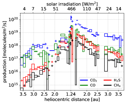
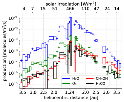
Figure 9: Surface emission rate $\dot{\rho}_{s,i,j}$ averaged over the patch $A_{4}$. The top axis denotes the diurnally and area-averaged solar irradiation on patch $A_{4}$. Left panel: CO₂, CO, H₂S, CH₄, right panel: H₂O, O₂, CH₃OH, H₂CO.

The analysis for the global production rates $Q_{s}$, e.g. as shown in Figure 2 of Läuter et al. ⁹, is complemented by the analysis of the surface emission rates $\dot{\rho}_{s,i,j}$ (see Section 2) averaged over the most active patch $A_{4}$ in Figure 9. On the same patch, the production of H₂O (as well as other gases like O₂, CH₃OH, H₂CO) diminishes faster than for CO₂, especially for heliocentric distances exceeding 2.5 au. This finding is related to the increasing heliocentric distance and the retreat of the subsolar latitude to the northern hemisphere (see Figure 4), which reduce the average radiation below $50~{}\mathrm{W}/\mathrm{m}^{2}$ and shut down the water sublimation (Figure 8).

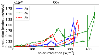
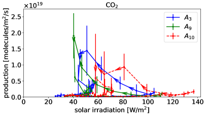
Figure 10: Surface emission rate $\dot{\rho}_{\mathrm{CO}_{2},i,j}$ averaged over patches as a function of diurnally averaged solar irradiation, inbound orbital arc, around perihelion and outbound orbital arc. The arrows denote the chronological sequence of the data points. The data points are connected to guide the eye. Left panel: on the southern hemisphere patches A₁, A₄, and A₆, right panel: on the northern hemisphere patches A₃, A₉, and A₁₀.

Similar to the evolution on patch A₄, each patch undergoes a specific temporal evolution of the solar irradiation on the one hand and of the gas production on the other hand. The relation between irradiation and observed sublimation rate can be viewed as an effective sublimation curve. Figure 10, left panel, shows the effective sublimation of CO₂ for the three most active patches A₁, A₄, and A₆ in the southern hemisphere. Around perihelion the patches receive a maximum irradiation between $300\,\mathrm{W}/\mathrm{m}^{2}$ and $450\,\mathrm{W}/\mathrm{m}^{2}$, which coincides with the maximum CO₂ production. The relationship between the diurnally averaged radiation and the gas production is non-linear before and after perihelion and shows a hysteresis effect when one traces the production chronologically. The arrows in Figure 10 connect consecutive observation times and show that the same amount of solar irradiation for the inbound and outbound orbital arcs lead to a higher gas production at the outbound arc. The right panel of Figure 10 focuses on the northern patches A₃, A₉, and A₁₀. Toward perihelion passage the irradiation decreases and the CO₂ production increases, see also Figure 4 in Läuter et al. ⁹. This indicates a failure for thermophysical models driven only by the instantaneous irradiation for the gas sublimation and requires a more comprehensive model. Additional parameters possibly include diurnal and seasonal retardation effects and the consideration of back falling material. Most COPS/DFMS measurements originate from terminator orbits, and therefore the measured densities do not sample the local time equally over one rotation, but preferentially from local morning and evening times. Only for a linear relationship between instantaneous solar irradiation and sublimation, the morning and evening conditions correspond to a diurnal mean of the gas production.

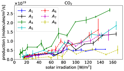
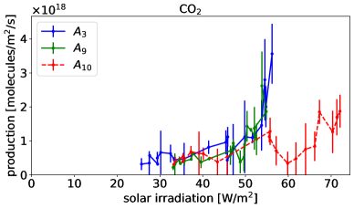
Figure 11: Surface emission rate $\dot{\rho}_{\mathrm{CO}_{2},i,j}$ averaged over patches as a function of diurnally averaged solar irradiation, between 100 days after and 390 days after perihelion. The data points are connected to guide the eye. Left panel: patches A₁, A₂, A₄–A₈ right panel: patches A₃, A₉, A₁₀.

The minimal model used in this Section cannot explain the non-linear increase of the gas production around perihelion and the observed hysteresis. To circumvent this problem we restrict ourselves to the outbound orbital arc 100 days to 390 days after perihelion, where the minimal model yields a better agreement with the measurements. For all southern patches we observe an almost linear relationship between CO₂ production and irradiation, see the left panel of Figure 11. We quantify the effective surface active fraction $f_{p}$ by comparing the observed relation of irradiation and emission rate to the theoretical sublimation function $Z_{\mathrm{CO}_{2}}(I)$ at $f_{p}=1$ shown in Figure 8. To determine $f_{p}$ for each southern patch $p$, the sublimation function $Z_{\mathrm{CO}_{2}}(I)$ is multiplied with $f_{p}$ to reproduce the observed data $Z_{\mathrm{CO}_{2},p}(I)$ in Figure 11, namely to fit best the relation $f_{p}\cdot Z_{\mathrm{CO}_{2}}(I)=Z_{\mathrm{CO}_{2},p}(I)$. In our minimal parameters model $f_{p}$ signifies the sublimation activity from a patch (which includes all exhumed gases in the column beneath the surface) to the incoming solar irradiation with respect to a fully ice-covered surface used to compute Figure 8. On the patches $A_{1}$, $A_{2}$, $A_{4}$–$A_{8}$ this value ranges between 0.2% on $A_{8}$ and 0.8% on $A_{4}$. Filacchione et al. ⁵³ reported a fraction of 0.1% of the area to show spectral signatures of CO₂ ice on one region (red dot in Figure 3) located in the patch $A_{7}$ (Anhur).

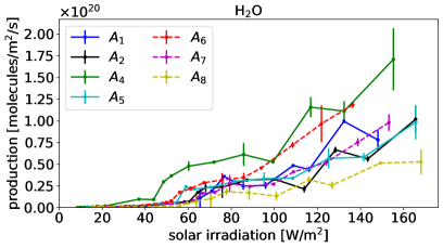
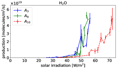
Figure 12: Surface emission rate $\dot{\rho}_{\mathrm{H}_{2}\mathrm{O},i,j}$ averaged over patches as a function of diurnally averaged solar irradiation, between 100 days after and 390 days after perihelion. The data points are connected to guide the eye. Left panel: patches A₁, A₂, A₄–A₈ right panel: patches A₃, A₉, A₁₀.

Figure 12 shows the H₂O productions for the period 100 days after perihelion for all patches. The analysis for H₂O shows similar hysteresis features as for CO₂ in Figure 10 and also shows an increasing emission for a decreasing irradiation on the northern patches. Quantitatively for H₂O both effects are smaller compared to CO₂. In contrast to CO₂, the water sublimation is sharply reduced to values below $10^{19}\,\mathrm{molecules}/\mathrm{m}^{2}/\mathrm{s}$ for irradiation smaller than $50\,\mathrm{W}/\mathrm{m}^{2}$. This is in agreement with the minimal thermophysical model for H₂O in Figure 8. The decline in water production occurs at heliocentric distances of 2.5 au–3 au ^{10, 45, 9}. The surface active fraction $f_{p}$ for H₂O is evaluated in the same way as for CO₂, by comparing the slopes in the Figure 12 to the reference with $f_{p}=1$ shown in Figure 8. On the patches $A_{1}$, $A_{2}$, $A_{4}$–$A_{8}$ this value ranges between 4% on $A_{8}$ and 15% on $A_{4}$.

The surface active fraction $f_{p}$ obtained from our thermophysical model can be put in context with independent estimates of the active area. Keller et al. ³⁶ include a fixed dust layer in the same model approach. They obtain fractions of the active surface between 6% and 25%, for the northern and southern hemisphere. Attree et al. ³⁸ consider a time varying surface active fraction in the range between 4% and 35% in different regions on the surface. Kramer et al. ⁴¹ estimate surface active fractions between 14% and 23% constrained by changes of the rotation axis. Filacchione et al. ²⁷ report fractions of the active area between 1% and 30% for water ice. Herny et al. ⁶⁷ require 20% active area to fit the water production within a complete orbit.

The evaluation of the surface active fraction for the species H₂O and CO₂ on the patches $A_{1}$, $A_{2}$, $A_{4}$–$A_{8}$ only works at times later than 100 days after perihelion. Then the monotonous relation between solar irradiation and emission rate allows us to apply the minimal thermophysical model. The northern patches $A_{3}$, $A_{9}$, and $A_{10}$ display a more complex behaviour during this time period and the emission rates cannot be explained within the minimal model. Additional factors might include the accumulation of dust (fallback).

5 Ice composition on hemispheres and on both lobes

The evolution of sublimation rates as a function of the received solar irradiation reflects a surface property which we have quantified as the surface active fraction with respect to one of the two major gases H₂O and CO₂. Another property we can derive from the observed ROSINA data is the ice composition close to the surface. The observed low water production for an average irradiation below $50\,\mathrm{W}/\mathrm{m}^{2}$ is linked to a change of the coma composition from a water dominated coma to a CO₂ dominated one 250 days after perihelion and later ^{56, 9}. The redeposition of dust onto the nucleus surface and the resulting layered structure of the nucleus material with different sublimation fronts for water and CO₂ causes relative abundances in the released gas which can differ from the ice composition within the nucleus ³⁰. Thus relative abundances of volatiles in the coma at a specific time may not reflect the ice composition of the nucleus directly ²⁷.

Independent of the temporal evolution of the gas composition, the “activity paradox” ^{68, 16, 5, 69} concerns the well known prevalence of a consistent and repetitive activity pattern over separated apparitions of a comet. While the sustained activity is an observed fact, the theoretical modeling of comets does not provide a simple mechanism to keep a comet active across multiple apparitions ⁶⁸. The main challenge is the continuous removal of the dry dust mantle, which is required to keep ices sublimating. Some models assume a time-independent thickness of a dust-layer ⁶⁰ or adapt an empirically chosen dust erosion rate to match the observation ^{65, 64}. In particular, the activity paradox refers to the limited understanding of the mechanisms for dust lift-off and fallback, and the dust composition. E.g. if the fallback was dry (without ice available for sublimation) it would cover the surface and the activity would be choked off. Consequently, a repeating emission rate across apparitions requires periodic and repetitive sublimation processes with similar molecular compositions and a largely unchanged ice composition. To quantify the ice composition in the nucleus from the ROSINA data in the coma requires additional assumptions.

One approach is to take the coma composition at a specific time close to perihelion passage ⁷⁰ as representative for the nucleus ice composition. Around perihelion the highest erosion rates are expected and deeper layers of material might be continuously exposed on the cometary surface. However, the sublimation rate is strongly affected by the local illumination conditions and the decoupling of CO₂ and H₂O sublimation leads to a variation of the relative abundances of the major and minor species in the coma over time. A second approach, and this is our assumption for this section, is to link the ice composition to the integrated gas emissions over an entire orbital period which we refer to as the orbital production of the gas. Even if the comet accumulates back falling material, the hypothesis of a repetitive activity across apparitions implies that fallback from a previous apparition will be shed off during the next one, and thus all sublimating materials are accounted for if one considers a complete orbital period. The pronounced maxima for the gas production around perihelion ⁹ lead to a significant representation of this time period as well. Thus the ice compositions of both approaches are comparable and within the range of the uncertainties of the gas production.

Our approach takes the relative mass-fractions of the orbital volatiles release to be representative of the ice composition close to the surface. The entire orbital production has not been directly measured and can only be approximated from the observed production ⁹ $P_{s}$ integrated over the mission time between 2014 and 2016. For all species we have estimated the uncertainty corresponding to the section of the orbital arc which was not covered by the Rosetta mission. The assumption of constant global outgassing based on the latest observed production rates in September 2016 yielded uncertainties in the range of the preexisting uncertainties for $P_{s}$ (see Table 1 in Läuter et al. ⁹). That is why we consider the observed production $P_{s}$ to be a good approximation for the orbital production.

$s$	$P_{s}(A_{\mathrm{SH}})/|A_{\mathrm{SH}}|~{}(\mathrm{kg}/\mathrm{m}^{2})$	$P_{s}(A_{\mathrm{NH}})/|A_{\mathrm{NH}}|~{}(\mathrm{kg}/\mathrm{m}^{2})$
H2O	$118\pm 22$	$65\pm 6$
CO2	$29\pm 7$	$4.9\pm 1.6$
CO	$5.3\pm 1.2$	$3.2\pm 0.8$
H2S	$4.4\pm 1.5$	$1.7\pm 0.6$
O2	$4.7\pm 1.0$	$2.7\pm 0.3$
C2H6	$2.1\pm 0.5$	$[4.8\pm 1.4]\times 10^{-1}$
CH3OH	$1.3\pm 0.3$	$[4.6\pm 0.9]\times 10^{-1}$
H2CO	$[9.5\pm 2.1]\times 10^{-1}$	$[4.6\pm 1.2]\times 10^{-1}$
CH4	$[4.8\pm 1.1]\times 10^{-1}$	$[2.1\pm 0.6]\times 10^{-1}$
NH3	$[4.0\pm 1.1]\times 10^{-1}$	$[2.8\pm 0.8]\times 10^{-1}$
HCN	$[3.4\pm 0.8]\times 10^{-1}$	$[1.6\pm 0.3]\times 10^{-1}$
C2H5OH	$[4.2\pm 1.1]\times 10^{-1}$	$[1.7\pm 0.3]\times 10^{-1}$
OCS	$[3.3\pm 0.8]\times 10^{-1}$	$[1.2\pm 0.3]\times 10^{-1}$
CS2	$[1.1\pm 0.2]\times 10^{-1}$	$[4.2\pm 1.1]\times 10^{-2}$

Table 3: Observed gas production $P_{s}$ per area for all species for the complete Rosetta mission time ranging from -377 days before to 390 days after perihelion. The gas production is given separately for the southern hemisphere $A_{\mathrm{SH}}$ (left column with the area $|A_{\mathrm{SH}}|=20.71\times 10^{6}\,\mathrm{m}^{2}$) and the northern hemisphere $A_{\mathrm{NH}}$ (right column with the area $|A_{\mathrm{NH}}|=23.60\times 10^{6}\,\mathrm{m}^{2}$).

Based on the values in Table 1 of Läuter et al. ⁹ and the entire surface area $|A_{\mathrm{67P}}|$ from Section 3 the accumulated production (the sum $\sum P_{r}$ over all species $r$) is $121\pm 13\,\mathrm{kg}/\mathrm{m}^{2}$. The same summations of the gas production (separately for both hemispheres in Table 3) leads to the observed production of $168\pm 23\,\mathrm{kg}/\mathrm{m}^{2}$ and $80\pm 6\,\mathrm{kg}/\mathrm{m}^{2}$ on the southern and on the northern hemisphere, $A_{\mathrm{SH}}$ and $A_{\mathrm{NH}}$, respectively. These significant differences are related to the higher irradiation of the southern hemisphere, since southern solstice occurs just 23 days after perihelion (see Figure 4).

Figures 13 and 14 visualize the production data for both hemispheres given in Table 3 and additionally they display the productions from the small and big lobes, $A_{\mathrm{SL}}$ and $A_{\mathrm{BL}}$. For both lobes, we find similar values for the observed productions, namely $129\pm 15\,\mathrm{kg}/\mathrm{m}^{2}$ on $A_{\mathrm{SL}}$ and $113\pm 12\,\mathrm{kg}/\mathrm{m}^{2}$ on $A_{\mathrm{BL}}$. We associate the relative mass-fractions of $P_{s}$ in the Figures 13 and 14 with the ice composition in the region of interest and deduce a similar composition of both lobes.

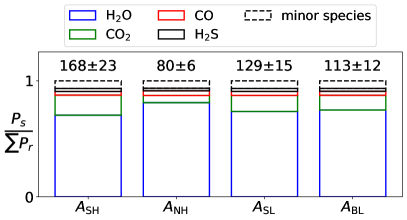
Figure 13: Observed gas production $P_{s}$ (integrated emission rates) over the entire 2015 apparition for the southern ($A_{\mathrm{SH}}$) and northern hemisphere $A_{\mathrm{NH}}$, and the small ($A_{\mathrm{SL}}$) and big lobe $A_{\mathrm{BL}}$, see Table 2. Mass-fraction of a species $P_{s}/\sum P_{r}$ is reflected by the segment size in the bar. On top of each bar, the sum (over the species) per area $\sum P_{r}/|A|~{}[\mathrm{kg}/\mathrm{m}^{2}]$ is given. The minor species cover O₂, C₂H₆, CH₃OH, H₂CO, CH₄, NH₃, HCN, C₂H₅OH, OCS, and CS₂ and are expanded in Figure 14.

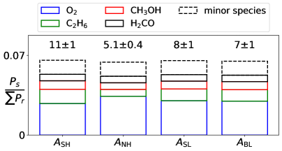
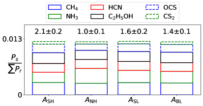
Figure 14: Observed production for minor species $P_{s}$ (integrated emission rates) over the entire 2015 apparition for the southern ($A_{\mathrm{SH}}$) and northern hemisphere $A_{\mathrm{NH}}$, and the small ($A_{\mathrm{SL}}$) and big lobe $A_{\mathrm{BL}}$, see Table 2. Mass-fraction of a species $P_{s}/\sum P_{r}$ is reflected by the segment size in the bar. On top of each bar, the sum (over the species) per area $\sum P_{r}/|A|~{}[\mathrm{kg}/\mathrm{m}^{2}]$ is given. Left panel: The minor species cover CH₄, NH₃, HCN, C₂H₅OH, OCS, and CS₂ which are given in the right panel.

Averaged over the complete surface the mass-fractions in the surface ice for H₂O and CO₂ are $74\pm 13\%$ and $13\pm 4\%$, respectively. These mass-fractions correspond to a ratio of $7\pm 2\%$ for CO₂/H₂O (taken as mole-fraction, see Table 1 in Läuter et al. ⁹). Based on the same DFMS data Combi et al. ⁴⁵ reported a CO₂/H₂O ratio of 7.3%. The CO₂/H₂O ratio changes with time (see Figure 5 in Läuter et al. ⁹) and can be compared with reported relative abundances at specific time periods. For April 2015 Migliorini et al. ⁷¹ give a value for the CO₂/H₂O ratio of 2.4%–3.9%, Fink et al. ⁷² report 3.7%–7.4% between February and April 2015, Rubin et al. ⁷ report $4.7\pm 1.4\%$ for May 2015, and Bockelée-Morvan et al. ¹¹ obtain 14%–32% between July and September 2015.

In addition to the reported difference of observed production on the southern and on the northern hemisphere, also the mass-fractions differ between both hemispheres. Based on the CO₂ values in Table 3 and Figure 13, the mass-fraction $6\pm 2\%$ in the ice on $A_{\mathrm{NH}}$ is decreased compared to $17\pm 5\%$ on $A_{\mathrm{SH}}$. This is related to CO₂/H₂O ratios (mole-fraction) of $3.1\pm 1.0\%$ on $A_{\mathrm{NH}}$ and $10\pm 3\%$ on $A_{\mathrm{SH}}$. The distinctive feature of a decreased CO₂ fraction on $A_{\mathrm{NH}}$ is also discussed by other authors ^{72, 11}. Without a conclusive explanation they claim that the surface ice on $A_{\mathrm{NH}}$ does not reflect the original composition of the nucleus. The illumination history could induce a stratified ice composition and affects a devolatilization process for CO₂ in the top layers ³². A complementing explanation points to lifted ice and dust particles due to surface gas activity (from the South) which later fall back in another region (in the North) due to their gravitational binding ^{73, 45, 74}. Similarly to water and CO₂, the mass-fractions (in relation to all ices) of the minor species O₂, C₂H₆, and NH₃ differ on $A_{\mathrm{SH}}$, with the values $2.8\pm 0.7\%$, $1.2\pm 0.3\%$ and $0.24\pm 0.07\%$, and on $A_{\mathrm{NH}}$, with the values $3.4\pm 0.5\%$, $0.6\pm 0.2\%$ and $0.35\pm 0.10\%$, respectively. On both lobes the mass-fractions for H₂O and CO₂ are almost identical, namely $74\pm 14\%$ and $14\pm 4\%$ on $A_{\mathrm{SL}}$ and $75\pm 13\%$ and $13\pm 3\%$ $A_{\mathrm{BL}}$, respectively. Similarly, the mass-fractions for all minor species shown in Figure 14 are comparable between both lobes.

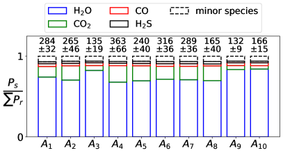
Figure 15: Observed gas production $P_{s}$ (integrated emission rates) over the entire 2015 apparition for the 10 patches in Table 2. Mass-fraction of a species $P_{s}/\sum P_{r}$ is reflected by the segment size in the bar. On top of each bar, the sum (over the species) per area $\sum P_{r}/|A|~{}[\mathrm{kg}/\mathrm{m}^{2}]$ is given. The minor species cover O₂, C₂H₆, CH₃OH, H₂CO, CH₄, NH₃, HCN, C₂H₅OH, OCS, and CS₂.

Averages over large regions (hemispheres and lobes) in the Figures 13 and 14 provide only the mean value of the gas productions in active areas. High resolution OSIRIS images and the VIRTIS spectroscopic analysis show small-scale areas holding ice-containing material (icy and ice-rich patches) which can be localized on the spatial scale of metres up to several tens of metres ^{51, 53, 50, 27}. With areas between $4\times 10^{5}~{}\mathrm{m}^{2}$ and $1.6\times 10^{6}~{}\mathrm{m}^{2}$, the consideration of the patches $A_{1}$–$A_{10}$ from Figure 3 allows us to increase the lower bounds for the observed production on the large regions in Figure 13. Figure 15 denotes the most active patches (with the highest observed production), namely $A_{4}$, $A_{6}$, $A_{7}$, $A_{1}$, and $A_{2}$, with production values of up to $363\pm 66\,\mathrm{kg}/\mathrm{m}^{2}$. Assuming a bulk density ¹⁵ of $538~{}\mathrm{kg}/\mathrm{m}^{3}$ this corresponds to an erosion due to ice sublimation of up to $0.7~{}\mathrm{m}$. The smallest observed productions within the set of patches occurs on the northern patches $A_{3}$ and $A_{9}$ with $135\pm 19\,\mathrm{kg}/\mathrm{m}^{2}$ and $132\pm 9\,\mathrm{kg}/\mathrm{m}^{2}$ which corresponds to a $0.2~{}\mathrm{m}$ height loss. Additional dust components increase the height loss depending on the dust-to-ice ratio in the nucleus. The averaged loss of 0.55 m height for cometary material ⁷⁵ (ice and dust) shows the difference between very local changes and the gas release averaged over larger areas. The higher productions across patches located on the southern hemisphere (compared to the ones located on the northern hemisphere) corresponds to the higher overall gas production on the entire southern hemisphere $A_{\mathrm{SH}}$, shown in Figure 13.

In Figure 15 within the group of all southern patches $A_{1}$, $A_{2}$, $A_{4}$–$A_{8}$ the mass-fractions for H₂O and CO₂ vary between $68\pm 21\%$ and $20\pm 7\%$ on A₄ and $74\pm 13\%$ and $13\pm 5\%$ on A₁, respectively. The corresponding CO₂/H₂O ratios (mole-fraction) range between $7\pm 3\%$ on A₁ and $12\pm 5\%$ on A₄ close to the averaged value on $A_{\mathrm{SH}}$. This agreement across patches also prevails on the northern hemisphere which is expressed in low mass-fractions of CO₂ between $4.1\pm 2.9\%$ on $A_{10}$ and $6\pm 3\%$ on $A_{3}$ (related to CO₂/H₂O mole-fractions between $2.0\pm 1.4\%$ and $3.0\pm 1.7\%$).

6 Conclusion

We have derived spatial maps of the emission rates on the surface of comet 67P/C-G, augmenting the globally integrated gas production given in Läuter et al. ⁹. Due to the uncertainties of the forward model and the partially limited surface coverage by measurement data, the spatial resolution of the grid ($\sim 120~{}\mathrm{m}$) provides only a lower bound for the resolution of the physical signal on the surface. The extracted spatial distribution of water emissions around perihelion leads us to identify 10 active patches on the surface with a typical size of $700~{}\mathrm{m}$ (the smallest patch is $4\times 10^{5}~{}\mathrm{m}^{2}$). 7 out of 10 patches are located on the southern hemisphere and all 10 patches (taken together) represent almost half of the global water emission. Both lobes of the concave surface harbor enhanced emission patches. The increased outgassing activity on the southern patches $A_{1}$, $A_{2}$, $A_{4}$–$A_{8}$ is not limited to H₂O emissions only, but goes hand in hand with enhanced emission of CO₂, CO and O₂ ²⁴ and also of all minor species analyzed here.

The analysis of gas emissions for different times and for different patches confirms the qualitative relationship between solar irradiation on the one hand and gas emission on the surface on the other hand. Our quantitative study of the emissions on the cometary surface is suitable for the validation of thermophysical models on comet 67P/C-G. The non-linear characteristic of such a model holds the property, that diurnally averaged irradiation might not be sufficient to describe observed emission rates. Periodic condensation of water in the surface layer can change insolation properties and thus delimit sublimation during night time when the interior is warmer ⁷⁶. Our analysis relates solar irradiation and emission rates and reveals complex phenomena depending on material properties (ice composition and dust fraction) and possibly on a global redistribution of dust from the South to the North. A hysteresis effect on the seasonal scale yields increased CO₂ emissions during the outbound orbit compared to the inbound phase with corresponding irradiation. On the northern patches, the maximum CO₂ emission does not coincide with the local maximum irradiation condition.

We established a minimal thermophysical model for the outbound orbital arc starting 100 days after perihelion, which allows one to determine the surface active fractions of H₂O and CO₂ on the southern patches. The CO₂ emission follows an almost linear relation with irradiation, which can be used to obtain the fraction of the active surface in the range of 0.2% and 0.8%. For H₂O, the sublimation requires higher irradiation exceeding $50~{}\mathrm{W}/\mathrm{m}^{2}$, which is seen in the data. We determine a fraction of the active surface for water between 4% and 15%.

Due to the complexity of the thermophysical processes on the surface and within the layers below, the ice composition is probably not reflected by the relative abundances in the instantaneous gas emissions. The observation of the “activity paradox”, a repetitive activity over several apparitions, relies on the assumption that the emission rates, integrated in time (gas production), serve as a good quantification for the ice composition. Our large scale analysis confirms the known phenomenon that gas production on comet 67P/C-G is predominantly located in the southern hemisphere, with twice as much gas production as in the northern hemisphere during the two-year mission time. During the same time the southern hemisphere received 1.4 as much solar irradiation as the northern one. Our method based on a localization on patches yields a lower estimate of $363\pm 66~{}\mathrm{kg}/\mathrm{m}^{2}$ for localized peak production during one apparition. This corresponds to a height loss of $0.7~{}\mathrm{m}$ due to ice sublimation only. On the northern hemisphere the mass-fraction of CO₂ in the ice close to the surface is $6\pm 2\%$ which goes down to $4.1\pm 2.9\%$ on the northern patch A₁₀. This is in contrast to the higher CO₂ mass-fractions, $13\pm 4\%$ globally averaged (corresponds to a mole-fraction of $7\pm 2\%$ for CO₂/H₂O) and $17\pm 5\%$ on the southern hemisphere. A maximum mass-fraction of $20\pm 7\%$ for CO₂ in the ice material is found on the southern patch A₄. In addition the minor species O₂, C₂H₆, and NH₃ change their mass-fractions in the ice from the northern hemisphere with the values $3.4\pm 0.5\%$, $0.6\pm 0.2\%$, and $0.35\pm 0.10\%$ to the southern hemisphere with the values $2.8\pm 0.7\%$, $1.2\pm 0.3\%$, and $0.24\pm 0.07\%$, respectively. The asymmetric irradiation conditions for both hemispheres, with southern solstice occurring 23 days after perihelion, lead to a redistribution of surface material, including dust and ice. Outgassing during the transfer of material from the southern to the northern hemisphere suggests that CO₂ is not a significant component in the deposited fallback ⁷⁴. On the northern hemisphere, CO₂ is subjected to longer lasting sublimation processes during the orbital arc around aphelion, which might partially deplete northern reservoirs of CO₂ ices. For the small and the big lobe, the comparisons of total gas production and of mass-fraction in the ice close to the surface do not show significant differences.

Appendix

The Appendix contains maps of the surface emission rates for additional species not shown in the main text or in Läuter et al. ²⁴. Läuter et al. ²⁴ displays surface emissions for the major species H₂O, CO₂, CO, O₂. Section 3 describes the surface emissions of H₂S, CH₄, CH₃OH, and H₂CO (Figures 5, 6, and 7). Emission maps for all remaining species C₂H₆, NH₃, HCN, C₂H₅OH, OCS, and CS₂ in all three time intervals $I_{\mathrm{inbound}}$, $I_{\mathrm{ph}}$, and $I_{\mathrm{outbound}}$ are shown in the Figures 16, 17, and 18.

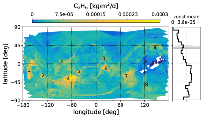
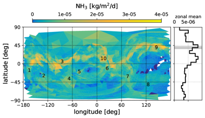
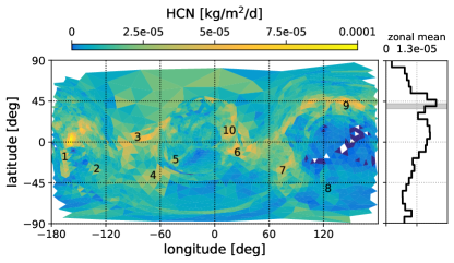
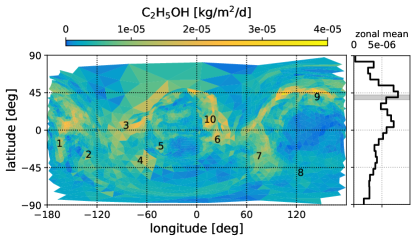
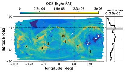
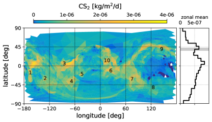
Figure 16: Surface emission rates for the minor gas species C₂H₆, NH₃, HCN, C₂H₅OH, OCS, and CS₂, averaged from 330 days to 270 days before perihelion, see $I_{\mathrm{inbound}}$ in Table 1.

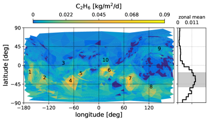
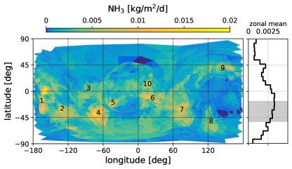
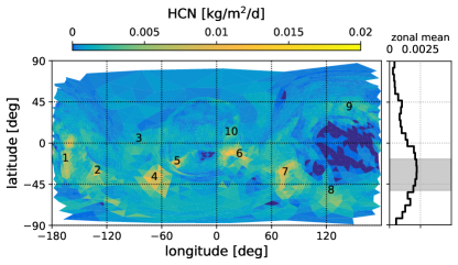
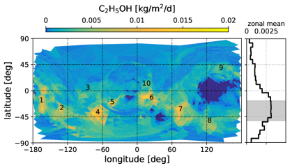
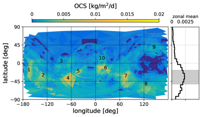
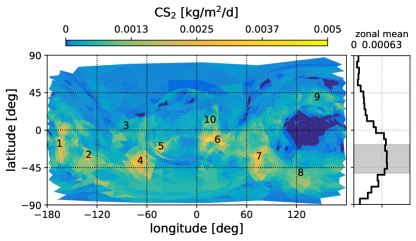
Figure 17: Surface emission rates for the minor gas species C₂H₆, NH₃, HCN, C₂H₅OH, OCS, and CS₂, averaged from 50 days before to 50 days after perihelion, see $I_{\mathrm{ph}}$ in Table 1.

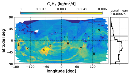
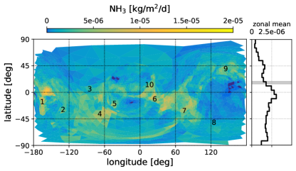
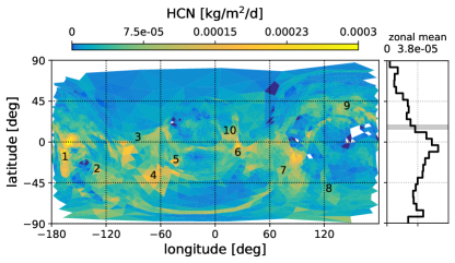
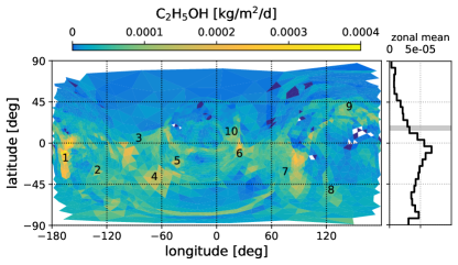
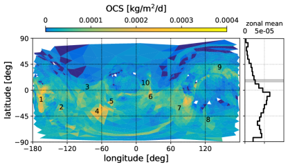
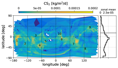
Figure 18: Surface emission rates for the minor gas species C₂H₆, NH₃, HCN, C₂H₅OH, OCS, and CS₂, averaged from 340 days to 390 days after perihelion, see $I_{\mathrm{outbound}}$ in Table 1.

References

- Geiss 1987 Geiss, J. Composition Measurements and the History of Cometary Matter. Astronomy and Astrophysics 1987, 187, 859–866
- Mumma and Charnley 2011 Mumma, M. J.; Charnley, S. B. The Chemical Composition of Comets—Emerging Taxonomies and Natal Heritage. Annual Review of Astronomy and Astrophysics 2011, 49, 471–524
- Altwegg et al. 2019 Altwegg, K.; Balsiger, H.; Fuselier, S. A. Cometary Chemistry and the Origin of Icy Solar System Bodies: The View After Rosetta. Annual Review of Astronomy and Astrophysics 2019, 57, 113–155
- Schulz 2009 Schulz, R. Rosetta – One Comet Rendezvous and Two Asteroid Fly-Bys. Solar System Research 2009, 43, 343–352
- Keller and Kührt 2020 Keller, H. U.; Kührt, E. Cometary Nuclei-From Giotto to Rosetta. Space Science Reviews 2020, 216, 14
- Balsiger et al. 2007 Balsiger, H. et al. Rosina – Rosetta Orbiter Spectrometer for Ion and Neutral Analysis. Space Science Reviews 2007, 128, 745–801
- Rubin et al. 2019 Rubin, M. et al. Elemental and Molecular Abundances in Comet 67P/Churyumov-Gerasimenko. Monthly Notices of the Royal Astronomical Society 2019, 489, 594–607
- Rubin et al. 2019 Rubin, M.; Bekaert, D. V.; Broadley, M. W.; Drozdovskaya, M. N.; Wampfler, S. F. Volatile Species in Comet 67P/Churyumov-Gerasimenko: Investigating the Link from the ISM to the Terrestrial Planets. ACS Earth and Space Chemistry 2019, 3, 1792–1811
- Läuter et al. 2020 Läuter, M.; Kramer, T.; Rubin, M.; Altwegg, K. The Gas Production of 14 Species from Comet 67P/Churyumov-Gerasimenko Based on DFMS/COPS Data from 2014-2016. Monthly Notices of the Royal Astronomical Society 2020, 498, 3995–4004
- Biver et al. 2019 Biver, N. et al. Long-Term Monitoring of the Outgassing and Composition of Comet 67P/Churyumov-Gerasimenko with the Rosetta/MIRO Instrument. Astronomy & Astrophysics 2019, 630, A19
- Bockelée-Morvan et al. 2016 Bockelée-Morvan, D. et al. Evolution of CO2, CH4, and OCS Abundances Relative to H2O in the Coma of Comet 67P around Perihelion from Rosetta/VIRTIS-H Observations. Monthly Notices of the Royal Astronomical Society 2016, 462, S170–S183
- Hässig et al. 2015 Hässig, M. et al. Time Variability and Heterogeneity in the Coma of 67P/Churyumov-Gerasimenko. Science 2015, 347, aaa0276
- Keller et al. 2007 Keller, H. U. et al. OSIRIS – The Scientific Camera System Onboard Rosetta. Space Science Reviews 2007, 128, 433–506
- Sierks et al. 2015 Sierks, H. et al. On the Nucleus Structure and Activity of Comet 67P/Churyumov-Gerasimenko. Science 2015, 347, aaa1044–aaa1044
- Preusker et al. 2017 Preusker, F. et al. The Global Meter-Level Shape Model of Comet 67P/Churyumov-Gerasimenko. Astronomy & Astrophysics 2017, 607, L1
- Vincent et al. 2019 Vincent, J.-B.; Farnham, T.; Kührt, E.; Skorov, Y.; Marschall, R.; Oklay, N.; El-Maarry, M. R.; Keller, H. U. Local Manifestations of Cometary Activity. Space Science Reviews 2019, 215, 30
- Cordiner et al. 2014 Cordiner, M. A. et al. Mapping the Release of Volatiles in the Inner Comae of Comets C/2012 F6 (Lemmon) and C/2012 S1 (Ison) Using the Atacama Large Millimeter/Submillimeter Array. The Astrophysical Journal 2014, 792, L2
- Farnham et al. 2021 Farnham, T. L.; Knight, M. M.; Schleicher, D. G.; Feaga, L. M.; Bodewits, D.; Skiff, B. A.; Schindler, J. Narrowband Observations of Comet 46P/Wirtanen during Its Exceptional Apparition of 2018/19. I. Apparent Rotation Period and Outbursts. The Planetary Science Journal 2021, 2, 7
- Bonev et al. 2021 Bonev, B. P. et al. First Comet Observations with NIRSPEC-2 at Keck: Outgassing Sources of Parent Volatiles and Abundances Based on Alternative Taxonomic Compositional Baselines in 46P/Wirtanen. The Planetary Science Journal 2021, 2, 45
- Cordiner et al. 2020 Cordiner, M. A.; Milam, S. N.; Biver, N.; Bockelée-Morvan, D.; Roth, N. X.; Bergin, E. A.; Jehin, E.; Remijan, A. J.; Charnley, S. B.; Mumma, M. J.; Boissier, J.; Crovisier, J.; Paganini, L.; Kuan, Y.-J.; Lis, D. C. Unusually High CO Abundance of the First Active Interstellar Comet. Nature Astronomy 2020, 4, 861–866
- Yang et al. 2021 Yang, B.; Li, A.; Cordiner, M. A.; Chang, C.-S.; Hainaut, O. R.; Williams, J. P.; Meech, K. J.; Keane, J. V.; Villard, E. Compact Pebbles and the Evolution of Volatiles in the Interstellar Comet 2I/Borisov. Nature Astronomy 2021, 5, 586–593
- Marschall et al. 2020 Marschall, R.; Skorov, Y.; Zakharov, V.; Rezac, L.; Gerig, S.-B.; Christou, C.; Dadzie, S. K.; Migliorini, A.; Rinaldi, G.; Agarwal, J.; Vincent, J.-B.; Kappel, D. Cometary Comae-Surface Links: The Physics of Gas and Dust from the Surface to a Spacecraft. Space Science Reviews 2020, 216
- Kramer et al. 2017 Kramer, T.; Läuter, M.; Rubin, M.; Altwegg, K. Seasonal Changes of the Volatile Density in the Coma and on the Surface of Comet 67P/Churyumov-Gerasimenko. Monthly Notices of the Royal Astronomical Society 2017, 469, S20–S28
- Läuter et al. 2019 Läuter, M.; Kramer, T.; Martin Rubin,; Altwegg, K. Surface Localization of Gas Sources on Comet 67P/Churyumov-Gerasimenko Based on DFMS/COPS Data. Monthly Notices of the Royal Astronomical Society 2019, 483, 852–861
- Haser 1957 Haser, L. Distribution d’intensité Dans La Tête d’une Comète. Bulletin de la Class des Sciences de l’Académie Royale de Belgique 1957, 43, 740–750
- Vincent et al. 2016 Vincent, J.-B. et al. Summer Fireworks on Comet 67P. Monthly Notices of the Royal Astronomical Society 2016, 462, S184–S194
- Filacchione et al. 2019 Filacchione, G.; Groussin, O.; Herny, C.; Kappel, D.; Mottola, S.; Oklay, N.; Pommerol, A.; Wright, I.; Yoldi, Z.; Ciarniello, M.; Moroz, L.; Raponi, A. Comet 67P/CG Nucleus Composition and Comparison to Other Comets. Space Science Reviews 2019, 215
- Vincent et al. 2021 Vincent, J.-B.; Kruk, S.; Fanara, L.; Birch, S.; Jindal, A. Automated Detection of Surface Changes on Comet 67P. EPSC Abstracts. 2021; pp EPSC2021–525
- Huebner and Benkhoff 1999 Huebner, W. F.; Benkhoff, J. In Composition and Origin of Cometary Materials; Altwegg, K., Ehrenfreund, P., Geiss, J., Huebner, W. F., Eds.; Springer Netherlands: Dordrecht, 1999; pp 117–130
- Huebner et al. 2006 Huebner, W.; Benkhoff, J.; Capria, M.-T.; A., C.; De Sanctis, C.; Orosei, R.; Prialnik, D. Heat and Gas Diffusion in Comet Nuclei; The International Space Science Institute: Bern, Switzerland, 2006
- Skorov and Blum 2012 Skorov, Y.; Blum, J. Dust Release and Tensile Strength of the Non-Volatile Layer of Cometary Nuclei. Icarus 2012, 221, 1–11
- Marboeuf and Schmitt 2014 Marboeuf, U.; Schmitt, B. How to Link the Relative Abundances of Gas Species in Coma of Comets to Their Initial Chemical Composition? Icarus 2014, 242, 225–248
- Groussin et al. 2019 Groussin, O. et al. The Thermal, Mechanical, Structural, and Dielectric Properties of Cometary Nuclei After Rosetta. Space Science Reviews 2019, 215, 29
- Prialnik 2020 Prialnik, D. Oxford Research Encyclopedia of Planetary Science; Oxford University Press, 2020
- Hoang et al. 2020 Hoang, M.; Garnier, P.; Lasue, J.; Rème, H.; Capria, M. T.; Altwegg, K.; Läuter, M.; Kramer, T.; Rubin, M. Investigating the Rosetta/RTOF Observations of Comet 67P/Churyumov-Gerasimenko Using a Comet Nucleus Model: Influence of Dust Mantle and Trapped CO. Astronomy & Astrophysics 2020, 638, A106
- Keller et al. 2015 Keller, H. U. et al. Insolation, Erosion, and Morphology of Comet 67P/Churyumov-Gerasimenko. Astronomy & Astrophysics 2015, 583, A34–A34
- Kramer and Läuter 2019 Kramer, T.; Läuter, M. Outgassing-Induced Acceleration of Comet 67P/Churyumov-Gerasimenko. Astronomy & Astrophysics 2019, 630, A4
- Attree et al. 2019 Attree, N.; Jorda, L.; Groussin, O.; Mottola, S.; Thomas, N.; Brouet, Y.; Kührt, E.; Knapmeyer, M.; Preusker, F.; Scholten, F.; Knollenberg, J.; Hviid, S.; Hartogh, P.; Rodrigo, R. Constraining Models of Activity on Comet 67P/Churyumov-Gerasimenko with Rosetta Trajectory, Rotation, and Water Production Measurements. Astronomy & Astrophysics 2019, 630, A18
- Mottola et al. 2020 Mottola, S.; Attree, N.; Jorda, L.; Keller, H. U.; Kokotanekova, R.; Marshall, D.; Skorov, Y. Nongravitational Effects of Cometary Activity. Space Science Reviews 2020, 216, 2
- Jorda et al. 2016 Jorda, L. et al. The Global Shape, Density and Rotation of Comet 67P/Churyumov-Gerasimenko from Preperihelion Rosetta/OSIRIS Observations. Icarus 2016, 277, 257–278
- Kramer et al. 2019 Kramer, T.; Läuter, M.; Hviid, S.; Jorda, L.; Keller, H.; Kührt, E. Comet 67P/Churyumov-Gerasimenko Rotation Changes Derived from Sublimation-Induced Torques. Astronomy & Astrophysics 2019, 630, A3
- Gasc et al. 2017 Gasc, S.; Altwegg, K.; Fiethe, B.; Jäckel, A.; Korth, A.; Le Roy, L.; Mall, U.; Rème, H.; Rubin, M.; Hunter Waite, J.; Wurz, P. Sensitivity and Fragmentation Calibration of the Time-of-Flight Mass Spectrometer RTOF on Board ESA’s Rosetta Mission. Planetary and Space Science 2017, 135, 64–73
- Tenishev et al. 2008 Tenishev, V.; Combi, M.; Davidsson, B. A Global Kinetic Model for Cometary Comae: The Evolution of the Coma of the Rosetta Target Comet Churyumov-Gerasimenko throughout the Mission. The Astrophysical Journal 2008, 685, 659–677
- Hansen et al. 2016 Hansen, K. C. et al. Evolution of Water Production of 67P/Churyumov-Gerasimenko: An Empirical Model and a Multi-Instrument Study. Monthly Notices of the Royal Astronomical Society 2016, 462, S491–S506
- Combi et al. 2020 Combi, M.; Shou, Y.; Fougere, N.; Tenishev, V.; Altwegg, K.; Rubin, M.; Bockelée-Morvan, D.; Capaccioni, F.; Cheng, Y.-C.; Fink, U.; Gombosi, T.; Hansen, K. C.; Huang, Z.; Marshall, D.; Toth, G. The Surface Distributions of the Production of the Major Volatile Species, H2O, CO2, CO and O2, from the Nucleus of Comet 67P/Churyumov-Gerasimenko throughout the Rosetta Mission as Measured by the ROSINA Double Focusing Mass Spectrometer. Icarus 2020, 335, 113421
- Fougere et al. 2016 Fougere, N. et al. Direct Simulation Monte Carlo Modelling of the Major Species in the Coma of Comet 67P/Churyumov-Gerasimenko. Monthly Notices of the Royal Astronomical Society 2016, 462, S156–S169
- Fougere et al. 2016 Fougere, N. et al. Three-Dimensional Direct Simulation Monte-Carlo Modeling of the Coma of Comet 67P/Churyumov-Gerasimenko Observed by the VIRTIS and ROSINA Instruments on Board Rosetta. Astronomy & Astrophysics 2016, 588, A134–A134
- Narasimha 1962 Narasimha, R. Collisionless Expansion of Gases into Vacuum. Journal of Fluid Mechanics 1962, 12, 294–294
- Preusker et al. 2015 Preusker, F. et al. Shape Model, Reference System Definition, and Cartographic Mapping Standards for Comet 67P/Churyumov-Gerasimenko – Stereo-photogrammetric Analysis of Rosetta/OSIRIS Image Data. Astronomy & Astrophysics 2015, 583, A33–A33
- Oklay et al. 2017 Oklay, N. et al. Long-Term Survival of Surface Water Ice on Comet 67P. Monthly Notices of the Royal Astronomical Society 2017, 469, S582–S597
- Barucci et al. 2016 Barucci, M. A. et al. Detection of Exposed H2O Ice on the Nucleus of Comet 67P/Churyumov-Gerasimenko: As Observed by Rosetta OSIRIS and VIRTIS Instruments. Astronomy & Astrophysics 2016, 595, A102
- Fornasier et al. 2016 Fornasier, S. et al. Rosetta’s Comet 67P/Churyumov-Gerasimenko Sheds Its Dusty Mantle to Reveal Its Icy Nature. Science 2016, 354, 1566–1570
- Filacchione et al. 2016 Filacchione, G. et al. Seasonal Exposure of Carbon Dioxide Ice on the Nucleus of Comet 67P/Churyumov-Gerasimenko. Science 2016, 354, 1563–1566
- Marshall et al. 2017 Marshall, D. W.; Hartogh, P.; Rezac, L.; von Allmen, P.; Biver, N.; Bockelée-Morvan, D.; Crovisier, J.; Encrenaz, P.; Gulkis, S.; Hofstadter, M.; Ip, W.-H.; Jarchow, C.; Lee, S.; Lellouch, E. Spatially Resolved Evolution of the Local H 2 O Production Rates of Comet 67P/Churyumov-Gerasimenko from the MIRO Instrument on Rosetta. Astronomy & Astrophysics 2017, 603, A87–A87
- Shinnaka et al. 2017 Shinnaka, Y.; Fougere, N.; Kawakita, H.; Kameda, S.; Combi, M. R.; Ikezawa, S.; Seki, A.; Kuwabara, M.; Sato, M.; Taguchi, M.; Yoshikawa, I. Imaging Observations of the Hydrogen Coma of Comet 67P/Churyumov-Gerasimenko in 2015 September by the Procyon/Laica. The Astronomical Journal 2017, 153, 76–76
- Gasc et al. 2017 Gasc, S. et al. Change of Outgassing Pattern of 67P/Churyumov–Gerasimenko during the March 2016 Equinox as Seen by ROSINA. Monthly Notices of the Royal Astronomical Society 2017, 469, S108–S117
- El-Maarry et al. 2019 El-Maarry, M. R.; Groussin, O.; Keller, H. U.; Thomas, N.; Vincent, J.-B.; Mottola, S.; Pajola, M.; Otto, K.; Herny, C.; Krasilnikov, S. Surface Morphology of Comets and Associated Evolutionary Processes: A Review of Rosetta’s Observations of 67P/Churyumov–Gerasimenko. Space Science Reviews 2019, 215
- Fornasier et al. 2019 Fornasier, S. et al. Linking Surface Morphology, Composition, and Activity on the Nucleus of 67P/Churyumov-Gerasimenko. Astronomy & Astrophysics 2019, 630, A7
- Fornasier et al. 2021 Fornasier, S.; Bourdelle de Micas, J.; Hasselmann, P. H.; Hoang, H. V.; Barucci, M. A.; Sierks, H. Small Lobe of Comet 67P: Characterization of the Wosret Region with ROSETTA-OSIRIS. Astronomy & Astrophysics 2021, 653, A132
- Blum et al. 2017 Blum, J. et al. Evidence for the Formation of Comet 67P/Churyumov-Gerasimenko through Gravitational Collapse of a Bound Clump of Pebbles. Monthly Notices of the Royal Astronomical Society 2017, 469, S755–S773
- Attree et al. 2018 Attree, N.; Groussin, O.; Jorda, L.; Rodionov, S.; Auger, A.-T.; Thomas, N.; Brouet, Y.; Poch, O.; Kührt, E.; Knapmeyer, M.; Preusker, F.; Scholten, F.; Knollenberg, J.; Hviid, S.; Hartogh, P. Thermal Fracturing on Comets: Applications to 67P/Churyumov-Gerasimenko. Astronomy & Astrophysics 2018, 610, A76
- Hu et al. 2019 Hu, X.; Gundlach, B.; von Borstel, I.; Blum, J.; Shi, X. Effect of Radiative Heat Transfer in Porous Comet Nuclei: Case Study of 67P/Churyumov-Gerasimenko. Astronomy & Astrophysics 2019, 630, A5
- Gundlach et al. 2020 Gundlach, B.; Fulle, M.; Blum, J. On the Activity of Comets: Understanding the Gas and Dust Emission from Comet 67/Churyumov-Gerasimenko’s South-Pole Region during Perihelion. Monthly Notices of the Royal Astronomical Society 2020, 493, 3690–3715
- Davidsson 2021 Davidsson, B. J. R. Thermophysical Evolution of Planetesimals in the Primordial Disc. Monthly Notices of the Royal Astronomical Society 2021, 505, 5654–5685
- Davidsson et al. 2021 Davidsson, B. J. R.; Samarasinha, N. H.; Farnocchia, D.; Gutiérrez, P. J. Modelling the Water and Carbon Dioxide Production Rates of Comet 67P/Churyumov–Gerasimenko. Monthly Notices of the Royal Astronomical Society 2021, 509, 3065–3085
- Statella 2021 Statella, T. Estimating Spectral Photometric Properties of the 67P/Churyumov-Gerasimenko Comet Nucleus. Applied Geomatics 2021,
- Herny et al. 2021 Herny, C.; Mousis, O.; Marschall, R.; Thomas, N.; Rubin, M.; Pinzón-Rodríguez, O.; Wright, I. New Constraints on the Chemical Composition and Outgassing of 67P/Churyumov-Gerasimenko. Planetary and Space Science 2021, 200, 105194
- Blum et al. 2014 Blum, J.; Gundlach, B.; Mühle, S.; Trigo-Rodriguez, J. Comets Formed in Solar-Nebula Instabilities! – An Experimental and Modeling Attempt to Relate the Activity of Comets to Their Formation Process. Icarus 2014, 235, 156–169
- Ip 2021 Ip, W.-H. Oxford Research Encyclopedia of Planetary Science; Oxford University Press, 2021
- Rubin et al. 2020 Rubin, M.; Engrand, C.; Snodgrass, C.; Weissman, P.; Altwegg, K.; Busemann, H.; Morbidelli, A.; Mumma, M. On the Origin and Evolution of the Material in 67P/Churyumov-Gerasimenko. Space Science Reviews 2020, 216, 102
- Migliorini et al. 2016 Migliorini, A. et al. Water and Carbon Dioxide Distribution in the 67P/Churyumov-Gerasimenko Coma from VIRTIS-M Infrared Observations. Astronomy & Astrophysics 2016, 589, A45
- Fink et al. 2016 Fink, U. et al. Investigation into the Disparate Origin of CO2 and H2O Outgassing for Comet 67/P. Icarus 2016, 277, 78–97
- Fulle et al. 2019 Fulle, M.; Blum, J.; Green, S. F.; Gundlach, B.; Herique, A.; Moreno, F.; Mottola, S.; Rotundi, A.; Snodgrass, C. The Refractory-to-Ice Mass Ratio in Comets. Monthly Notices of the Royal Astronomical Society 2019, 482, 3326–3340
- Davidsson et al. 2021 Davidsson, B. J.; Birch, S.; Blake, G. A.; Bodewits, D.; Dworkin, J. P.; Glavin, D. P.; Furukawa, Y.; Lunine, J. I.; Mitchell, J. L.; Nguyen, A. N.; Squyres, S.; Takigawa, A.; Vincent, J.-B.; Zacny, K. Airfall on Comet 67P/Churyumov–Gerasimenko. Icarus 2021, 354, 114004
- Keller et al. 2017 Keller, H. U. et al. Seasonal Mass Transfer on the Nucleus of Comet 67P/Chuyumov-Gerasimenko. Monthly Notices of the Royal Astronomical Society 2017, 371, 357–371
- De Sanctis et al. 2015 De Sanctis, M. C. et al. The Diurnal Cycle of Water Ice on Comet 67P/Churyumov–Gerasimenko. Nature 2015, 525, 500–503