On Computing Universal Plans for Partially Observable Multi-Agent Path Finding

Abstract

Multi-agent routing problems have drawn significant attention nowadays due to their broad industrial applications in, e.g. warehouse robots, logistics automation, and traffic control. Conventionally they are modelled as classical planning problems. In this paper, we argue that it is beneficial to formulate them as universal planning problems. We therefore propose universal plans, also known as policies, as the solution concepts, and implement a system called ASP-MAUPF (Answer Set Programming for Multi-Agent Universal Plan Finding) for computing them. Given an arbitrary two-dimensional map and a profile of goals for the agents, the system finds a feasible universal plan for each agent that ensures no collision with others. We use the system to conduct some experiments, and make some observations on the types of goal profiles and environments that will have feasible policies, and how they may depend on agents’ sensors. We also demonstrate how users can customize action preferences to compute more efficient policies, even (near-)optimal ones.

1 Introduction

Consider a situation in a warehouse where a fleet of robots are programmed to deliver fragile packages to designated ports or shelves. The robots are supposed to reach their ports as fast as possible while avoiding any collisions with others. This setting can be formulated as a Multi-Agent Path Finding problem (MAPF), where a group of agents starts from a set of initial positions and find paths towards their dedicated goals without any collision (?; ?). Although optimally solving MAPF problems in principle is NP-hard (?), in practice there are planners that can efficiently find solutions and are applicable to some real-world domains in, e.g., warehouse logistics (?), complex robot teams (?; ?), traffic control (?), aviation (?) and even management of pipe systems (?).

In a controlled environment and with all agents under the control of a central system, the multi-agent routing problem as a MAPF instance makes sense. However, if there is a given uncertainty arising from the environment or the other agents, computing a path for each agent is not that useful as it needs to be re-computed in any unforeseen situation, which will be the norm under uncertainty. Thus, when there is uncertainty, the right solution concept should be in terms of functions that map from states to actions. These functions are called universal plans in planning (?), strategies in extensive-form games, and policies in Markov decision processes (MDPs).

In this paper, we present an ASP system called ASP-MAUPF (Answer Set Programming for Mutli-Agent Universal Plan Finding) for computing universal plans. The system assumes a grid world domain with multiple agents. The grid world may contain obstacles. Each agent knows the grid world, and has a goal location to go to, but does not know the other agents’ goal and their current locations unless they are within her field of view (FoV). Moreover, all agents are not equipped with any communication modules for message sharing. Basically, our system takes in a problem instance specified by a given map layout and a group of partially observable agents, translates it into ASP encodings, and computes a decentralized policy for each agent. In principle, once a policy profile is found, it works no matter where agents are placed initially and how they get perturbed during routing. A graphical illustration is shown in Figure 1. With the help of this system, we provide three case studies as follows.

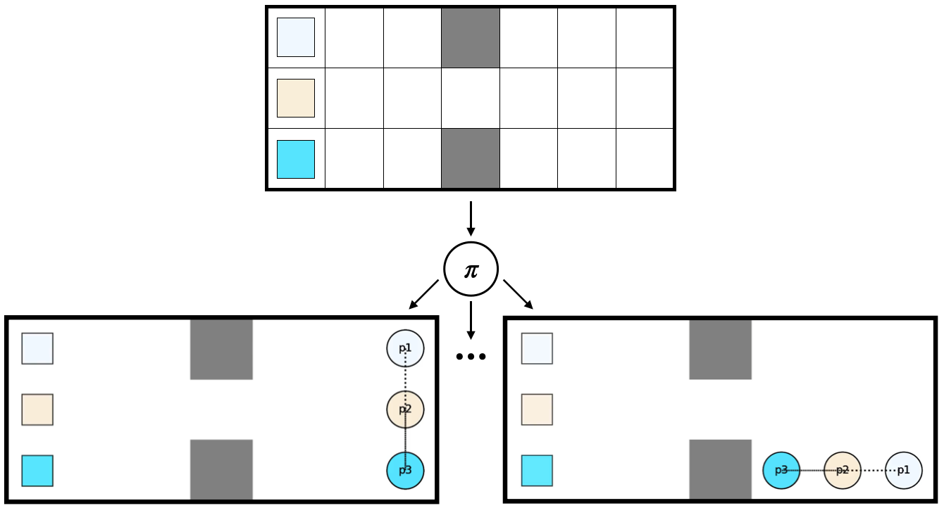
Figure 1: An example (two chambers connected by a tight hallway) that shows how our proposed policy-like solution works. Once computed (takes 167.35s for searching), it will be applicable for all 19*18*17 = 5814 global states. Colored squares are goals assigned to sphere shaped agents in corresponding colors.

Feasibility. A policy profile is feasible if all agents can achieve their goals without ever colliding with others. We test the efficiency of our system and report here the time cost for computing feasible policies for different sizes of configurations. Sometimes there may not be any feasible policy, and we therefore conduct experiments to show how the existence of feasible policies may depend on agents’ FoV.

Action restrictions. In addition to feasibility, one may also want to restrict the policies in certain ways. Our system provides two ways for the user to specify action restrictions. The first type of restrictions is imposed as each individual agent’s preferences over actions, e.g., an agent may prefer actions that would make her closer to the goal regardless of her observations. The second type of restrictions is represented as a type of common knowledge among all agents. This can be interpreted as traffic rules requiring agents to adopt a shared protocol when they meet each other. These action restrictions rule out undesirable policies, thus, can be an effective strategy for pruning the search space. It turns out to be a better way to generate more efficient policies than searching from scratch.

Anytime optimization. Modern ASP solvers allow us to compute optimized solutions in an anytime fashion. The longer the program keeps running, the better the returned solution will be. However, given the high complexity of the overall problem, we observe in our experiments that to compute better policies, it is computationally more practical to implement some heuristic functions through action restriction described above than to do it from scratch by brute-force, as we mentioned above.

The rest of the paper is organized as follows. Section 2 lists a number of related domains. After that, Section 3 presents the mathematical preliminaries to facilitate our illustration. Then, Section 4 elaborates on two formal encodings to address the problem. Section 5 follows by showing three insightful case studies. Finally, we conclude the paper by discussing potential applications of our system and possible future directions to work on.

2 Related Work

We list a few related areas that inspire our work but still we need to distinguish our work from those.

Compilation-based methods for MAPF. For conventional MAPF problems, apart from leveraging best-first search techniques (?), researchers also investigate methods that compile MAPF instances into formal languages and solve them by declarative programming. Success has been witnessed in formulations as SAT (?), CSP (?), SMT (?). In particular, we note that one can also formulate such problems in similar or variant setting in expressive nonmonotonic languages of Answer Set Programming (ASP), e.g., (?), (?) and (?). Nevertheless, the solution concept in their settings is still a sequence of joint actions for a group of agents from initial positions to goal positions. Our work in this paper aims at computing a universal plan, i.e. a profile of decentralized individual policies, each of which maps an agent’s local states (defined under partial observability) to available actions. The policy profile by our definition should work for any possible situation.

Universal planning. Another domain that highly matches ours is called universal planning in single-agent domains. ? (?) first motivates the investigation of the universal plan by an example of the well-known Blocks World, where a conventional planner may be bothered by a naughty baby who would occasionally smash down the built blocks, and therefore may need redundant replanning. The idea of universal planning in fact quite overlaps with contingent planning or planning under partial observability (?; ?). Work from those domains also desires policies or conditional plans to be the appropriate solution concept. Recent work like (?) has thoroughly investigated the idea of expressing policies by knowledge-based programs, where branching conditions are epistemic formulas (?), even in partially observable domains. Such solution concept can also be implemented by ASP towards cognitive robotics applications (?). More sophisticatedly, ? (?) has surveyed about the maturity and the drawback of utilizing ASP for planning problems.

Dec-POMDPs and MARL. The most popular related domain goes to Multi-agent Reinforcement Learning (MARL), especially for cooperative tasks. The underlying model is usually framed as Decentralized Partially Observable Markov Decision Processes (Dec-POMDP), which is a chain of state games where agents share the same utility function but are not fully aware of which state they are in (?; ?; ?). It is even undecidable to optimally solve infinite horizon Dec-POMDPs (?). Accordingly, there has been a vast amount of literature leveraging reinforcement learning techniques for approximation (?; ?). However, Dec-POMDPs require certain prior distributions over the initial states , and it models transitions as well as observations in a probabilistic fashion. Therefore, we argue that Dec-POMDP is still not the most suitable formulation for our problem.

3 Preliminaries

We consider an arbitrary map and a group of agents with partial observability. A configuration is a 3-tuple $<G,N,\bm{g}>$ defined as follows:

• $G=(E,V)$ is an unweighted undirected graph representing the underlying map, where $E$ denotes the set of vertices that agents can be positioned at and $V$ denotes the set of edges that agents can travel through. Usually, a two-dimensional real-world layout can be represented as a grid map up to some resolution. Without loss of generality, we just make $G$ a four-connected grid map with pre-specified obstacles.

• $N$ is a set of $n$ agents. Each agent is equipped with two functionalities $(A,R)$. $A$ denotes the set of actions. A feasible action moves an agent from node $i$ to node $j$, such that $(i,j)\in V$. $R$ denotes the sensor (e.g. radar) that is able to detect other agents in a local field of view (FoV). $R$ is said to be of sensor range $r$ if $R$ is capable of detecting $r$-hop neighbors. For example, given a four-connected grid map, agents are associated with five cardinal actions {$Up,Down,Left,Right,Stop$}. In such a grid map, for simplicity of illustration, a sensor of range $r$ enables agents at location $(x,y)$ to observe others at locations $\{(x^{\prime},y^{\prime}):|x-x^{\prime}|\leq r\land|y-y^{\prime}|\leq r\}$.

• $\bm{g}=(\bm{g_{1}},\cdots,\bm{g_{n}})$ is a goal profile, where $\bm{g}_{i}$ is the goal designated to agent $i$.

The functionalities therefore define the set of all possible local states of every agent $i$, denoted as $O_{i}$.

A collision happens when two agents knock into each other at the same vertex (vertex collision) or they traverse the same edge (edge collision). Mathematically, let $pos_{i}^{t}$ denote the vertex where agent $i$ is positioned at time step $t$, then a collision happens between agent $i$ and $j$ if

• $pos_{i}^{t}\in E\land pos_{j}^{t}\in E\land pos_{i}^{t}=pos_{j}^{t}$, or

• $(pos_{i}^{t},pos_{j}^{t})\in V\land(pos_{i}^{t+1},pos_{j}^{t+1})\in V\land(pos_{i}^{t},pos_{j}^{t})=(pos_{j}^{t+1},pos_{i}^{t+1})$.

An instantiation is to assign an initial profile $\bm{i}\in E^{N}$ to agents, where $\bm{i}_{i}$ is the initial position of agent $i$ and $\bm{i}_{i}\neq\bm{i}_{j},\forall i\neq j$. That is to say, any two agents cannot be placed at the same initial position. We desire a deterministic policy $\pi_{i}:O_{i}\mapsto A$ for each agent $i$, which is a mapping from the set of agent $i$’s local states to the set of actions. Given a configuration, a policy profile $\bm{\pi}=(\pi_{1},\cdots,\pi_{n})$ is said to be feasible if the following three conditions are satisfied for any possible instantiation,

1. No collision happens between any pair of agents.

2. Once an agent has reached her goal, she will stop and serve as a fixed obstacle.

3. All agents successfully reach their goals within finite time steps.

4 Formal Encoding

In this section, we formalize the problem in a fine-grained manner via Answer Set Programming (ASP). We address the problem by first finding feasible solutions and then incorporating optimization procedures.

4.1 Why ASP

We explain why we choose to encode the problem in ASP by discussing several potential alternatives.

1. Researchers can leverage reinforcement learning methods (?) to train a policy, but such reward-incentivized methods cannot guarantee a collision-free solution.

2. Solvers for infinite-horizon Dec-POMDPs (?; ?) can also be utilized. However, they can only solve very small problem instances, ones with only about dozens local states. Furthermore, they do not scale to more than two agents. In our settings, for a three-agent configuration under a $4\times 4$ map with sensors of range two, there are already nearly 2000 local states for each agent. So far as we know, problem instances of such scales are out of reach for Dec-PODMP solvers (even approximated ones). As we will see, our system can find a solution in a few minutes.

An added advantage of using ASP is that it enables us to easily axiomatize human-understandable logic to study the behavior of agents and therefore even polish the policy.

4.2 ASP Encoding

In this section, we propose a fine-grained encoding powered by ASP.

First, we encode the following preliminaries:

• cell(X,Y) and block(X,Y) encode the empty girds and obstacles on the map, respectively.

• goali((GX,GY)) specifies the goal designated to agent $i$.

• Actions are encoded as follows (similarly for down, right, left and nil).

  action(X,Y,up):-
      cell(X,Y), not block(X,Y),
      cell(X-1,Y), not block(X-1,Y).
      
  

Then we format the global state representation, which is a snapshot of the whole system including the current positions and the respective goals of all agents. Note that all agents are supposed to be placed at an empty cell and not to overlap with each other.

gState(S):- S=(L1,...,Ln,G1,...,Gn),
    goal1(G1), ..., goaln(Gn),
    % for all i
    L1=(Xi,Yi),
    cell(Xi,Yi), not block(Xi,Yi),
    % for all distinct i,j
    Li!=Lj.

Upon the definition of global states, we are able to define the transition. A global transition is triggered upon an action profile, which is a collection of all agents’ reported actions. Note that any pair of agents cannot traverse the same passage, i.e. no immediate swap is allowed.

trans(S1,A1,...,An,S2):-
    gState(S1), gState(S2),
    S1=(L11,...,L1n,G11,...,G1n),
    S2=(L21,...,L2n,G21,...,G2n),
    L11=(X11,Y11), ..., L1n=(X1n,Y1n),
    L21=(X21,Y21), ..., L2n=(X2n,Y2n),
    % for all i
    move(X1i,Y1i,Ai,X2i,Y2i),
    % for all distinct i,j
    (L1i,L1j)!=(L2j,L2i).

To make the system goal-directed, we also need to format the global goal state.

goal_gState(S):- gState(S),
    S=(G1,...,Gn,G1,...,Gn),
    goal1(G1), ..., goaln(Gn).

As we mentioned earlier, each agent is only capable of observing others within her local FoV.

aState(AS):-
    AS=(Self,O2,...,On,Goal),
    Self=(X,Y),
    cell(X,Y), not block(X,Y),
    Goal=(Xg,Yg),
    cell(Xg,Yg), not block(Xg,Yg),
    % for all i=2..n
    near(Self,Oi).

The near predicate denotes the functionality of the sensor. If the opponent is beyond the detection of the agent, we let the constant empty be the placeholder for such a null position. The constant R denotes the sensor range. One can alternatively adopt any other distance measure, e.g. Manhattan distance or Euclidean distance. For simplicity, our example represents a FoV of a square with a side length of R.

near(Self,empty):-
    Self=(X1,Y1), cell(X1,Y1).
near(Self,Other):-
    Self!=Other,
    Self=(X1,Y1), Other=(X2,Y2),
    |X1-X2|<=R, |Y1-Y2|<=R,
    cell(X1,Y1), not block(X1,Y1),
    cell(X2,Y2), not block(X2,Y2).

As required, each agent will not be incentivized to do any further move once she reaches the goal. Thus, each agent should be capable of recognizing her own dedicated goal.

goali_aState(AS):- aState(AS),
    AS=(G1,_,...,_,G1), goali(Gi).

To map from global states to each agent’s local states, we then define the observation model. Note that by (L1,...,Ln)$\backslash$Self we mean to exclude the agent herself from the vector of all agents’ locations. By empty/Oi we mean that the the $i$-th one of other agents can be outside or inside the FoV. Correspondingly, if Oi is not detected, then we include not near(Self,Oi), otherwise no leading not. The observation model is in fact the most expensive one to encode in our system, since we need to enumerate all possible $2^{n-1}$ situations of sensor detection for each agent, thus, $n\cdot 2^{n-1}$ axioms in total.

obsi(S,AS):-
    gState(S), S=(L1,...,Ln,G1,...,Gn),
    Self=Li,
    (O2,...,On)=(L1,...,Ln)\Self,
    aState(AS),
    AS=(Self,empty/O2,...,empty/On,Gi),
    % for all i=2..n
    {not} near(Self,Oi).

On top of the above, we therefore formulate the policy under two restrictions: 1) once an agent reaches her dedicated goal, she has to stop; 2) pick one single available action otherwise. Our desired solution is consequently a deterministic one and reasonable from the local perspective of an agent.

doi(AS,nil):- goali_aState(AS).
{doi(AS,A): avai_action(AS,A)}=1 :-
    aState(AS), AS=(Self,_,...,_,Goal),
    Self != Goal, goali(Goal).

To ensure that the policy works for every contingency, we inductively define the reachability of each global state given the policy. Basically, a goal global state is trivially reachable to itself. Inductively, any global state is reachable to the goal state if it can, according to the policy, transit to a successor state that is reachable to goal state.

reached(S):- goal_gState(S).
reached(S1):- gState(S1),
    % for all i
    obsi(Si,ASi), doi(ASi,Ai),
    trans(S1,A1,...,An,S2),
    reached(S2).

Finally, we include the integrity constraint to rule out infeasible policies.

:- gState(S), not reached(S).

It should be clear that given an answer set of a logic program as defined above, the policy profile encoded in the answer set by the do predicate will be a feasible one. Conversely, one can construct an answer set from a feasible policy profile. In other words, our ASP implementation is both sound and complete.

For optimization, there are quite a few evaluation criteria for the conventional MAPF problem. However, none of them fit in our settings, since we desire a policy for all contingencies. Instead, we adopt a criterion called minimizing sum-of-makespan, which adds up the makespans of all instantiations under the execution of the policy. Mathematically,

$$\textit{sum-of-makespan}(\bm{\pi})=\sum_{\bm{i}\in E^{N}:\bm{i}_{i}\neq\bm{i}_{j}}\textit{makespan}(\bm{i},\bm{\pi}).$$

The so called makespan is defined as the number of steps of the longest path among those of all the agents. In fact, given a policy the makespan coincides with the number of global transitions made from the initial global state to reach the goal global state. Therefore, we can also axiomatize makespan inductively as follows, denoted as the dist predicate. Every global state is associated with a non-negative cost, which will be incremented by one upon a global transition according to the policy.

w(0..UPPERBOUND).
dist(S,0):- goal_gState(S).
dist(S1,C):- not goal_gState(S1),
    % for all i
    obsi(Si,ASi), doi(ASi,Ai),
    trans(S1,A1,...,An,S2),
    reached(S1), dist(S2,C-1), w(C).
#minimize {C, dist(S,C): dist(S,C)}.

Eventually, we emphasize that the computed policy is a deterministic and decentralized one, in the sense that once it is deployed on individual agents, no further interference from the central controller is needed.

5 Case Studies

In this section, we categorize our case studies into three folds. Basically, the spectrum is from feasibility to optimality.

First, we merely look at feasible policies. For users’ reference, we report the time elapse to compute feasible policies for different sizes of configurations. On top of that, systematic experiments are designed to investigate how feasibility depends on agents’ FoV. We leave the formal characterization to future work.

Second, we restrict the choice of actions of agents to see if there still exists a feasible policy. Restrictions can happen either when agents detect no others, or when agents do detect some of the others. When the environment is large and sparse, once we have set appropriate action preferences, the system is already efficient enough, to some extent, since most of the time they do not need to compromise on their preferences.

Finally, we look at the optimization of the policy. A natural idea is to encode the metric sum-of-makespan as mentioned earlier. We show two alternatives to achieve the objective. For one, we directly keep the ASP solver running until it finds better and better solutions, which is probably time consuming. For the other, we manually design part of the policy according to previous findings and leave the work of finding efficient ways of coordination to the solver. Note that, the second alternative only finds optimal solutions confined to the manually designed part, while the first alternative intends to find the ground-truth (i.e. the globally optimal ones).

5.1 Feasibilities

Computational Time

For a rough analysis of the time complexity, each agent is associated with around $M{\binom{K+n-1}{n-1}}$ local states, where $M$ denotes the number of all possible positions which an agent can be placed at and $K$ denotes the number of neighboring cells that an agent can detect . For example, for a $4\times 4$ map with three agents, all are equipped with sensors of range two, then each agent will be associated with around 2000 local states, which is an intractable scale for Dec-POMDP solvers.

We report in Table 1 the time elapse for computing a feasible policy. Programs are solved by clingo  (?; ?) and all experiments are done on Linux servers with Intel(R) Xeon(R) Silver 4210 CPU @ 2.20GHz. Sensor i means the that agents are equipped with sensors of range $i$ . It is observed that for a given map different goal locations affect the computational time subtly, therefore, the results are collected from one single goal profile for each configuration.

Map size	2 agents	3 agents	4 agents	5 agents
Sensor 1
$3\times 3$	0.06s	3.23s	6.09min	8.76hr
$4\times 4$	0.29s	5.09min	28.40hr	$/$
$5\times 5$	1.61s	40.24min	$/$	$/$
$6\times 6$	11.69s	6.02hr	$/$	$/$
Sensor 2
$3\times 3$	0.06s	3.51s	8.86min	8.47hr
$4\times 4$	0.49s	2.22min	15.60hr	$/$
$5\times 5$	2.30s	24.02min	$/$	$/$
$6\times 6$	7.50s	4.14hr	$/$	$/$
Sensor 3
$3\times 3$	0.10s	3.37s	9.00min	8.92hr
$4\times 4$	0.39s	2.42min	18.69hr	$/$
$5\times 5$	2.07s	26.71min	$/$	$/$
$6\times 6$	7.54s	4.46hr	$/$	$/$

Table 1: Computational time for varying maps, numbers of agents and sensors. Sensor i means the agents are equipped with sensors of range $i$.

Existence of Feasible Policies

Apart from the situations where we do find feasible policies, there are certain scenarios where no feasible policy exists. Map layouts, type of sensors and placement of goals all matters.

Definition 1.

Given a map $G$, a goal profile $\bm{g}$ is said to be proper, if for any $\bm{g}_{i}$, there is always a path from any other positions $v\in G\backslash\bm{g}_{-i}$ to $\bm{g}_{i}$, without passing through any other $\bm{g}_{-i}$.

There exists a feasible policy only if the goal profile is proper. This necessary condition is easy to prove. Note that agents are not supposed to move any longer once they reach their own goals. If the given goal profile is not proper, then if certain agents are initialized right at their goals, there is no chance for the rest to reach their goals.

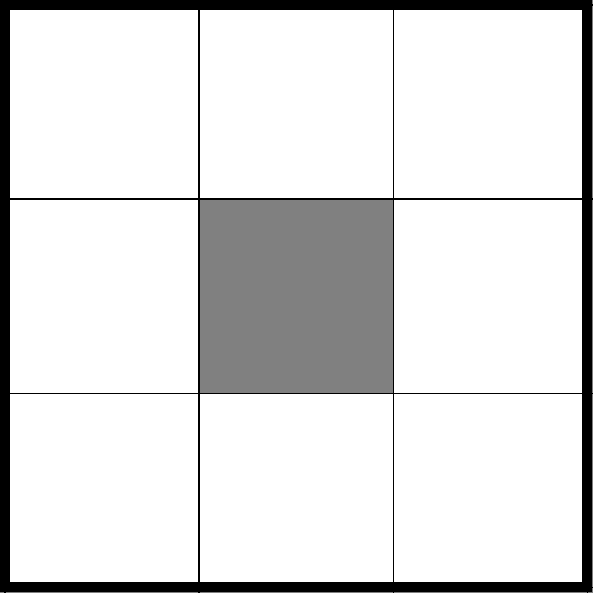
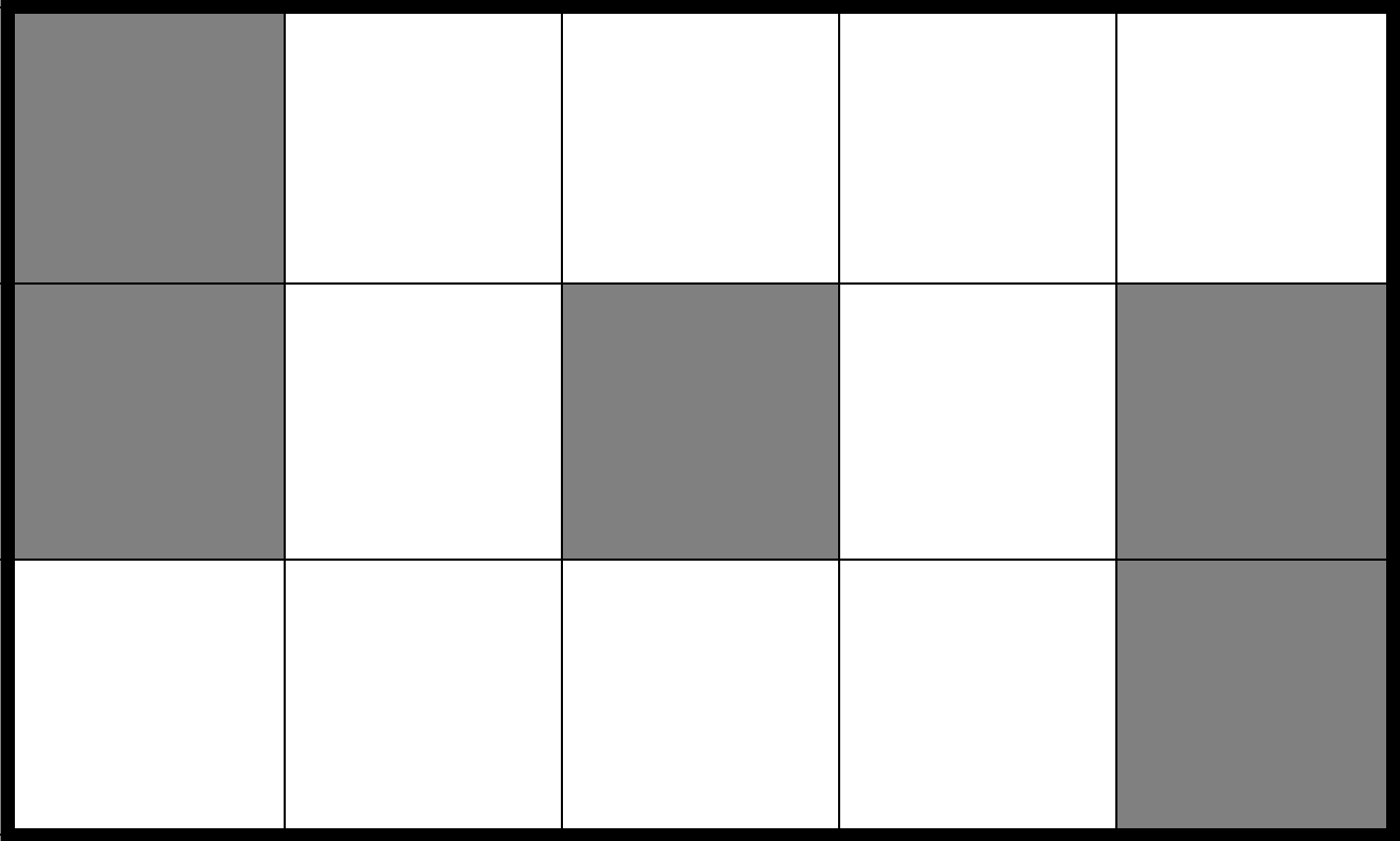
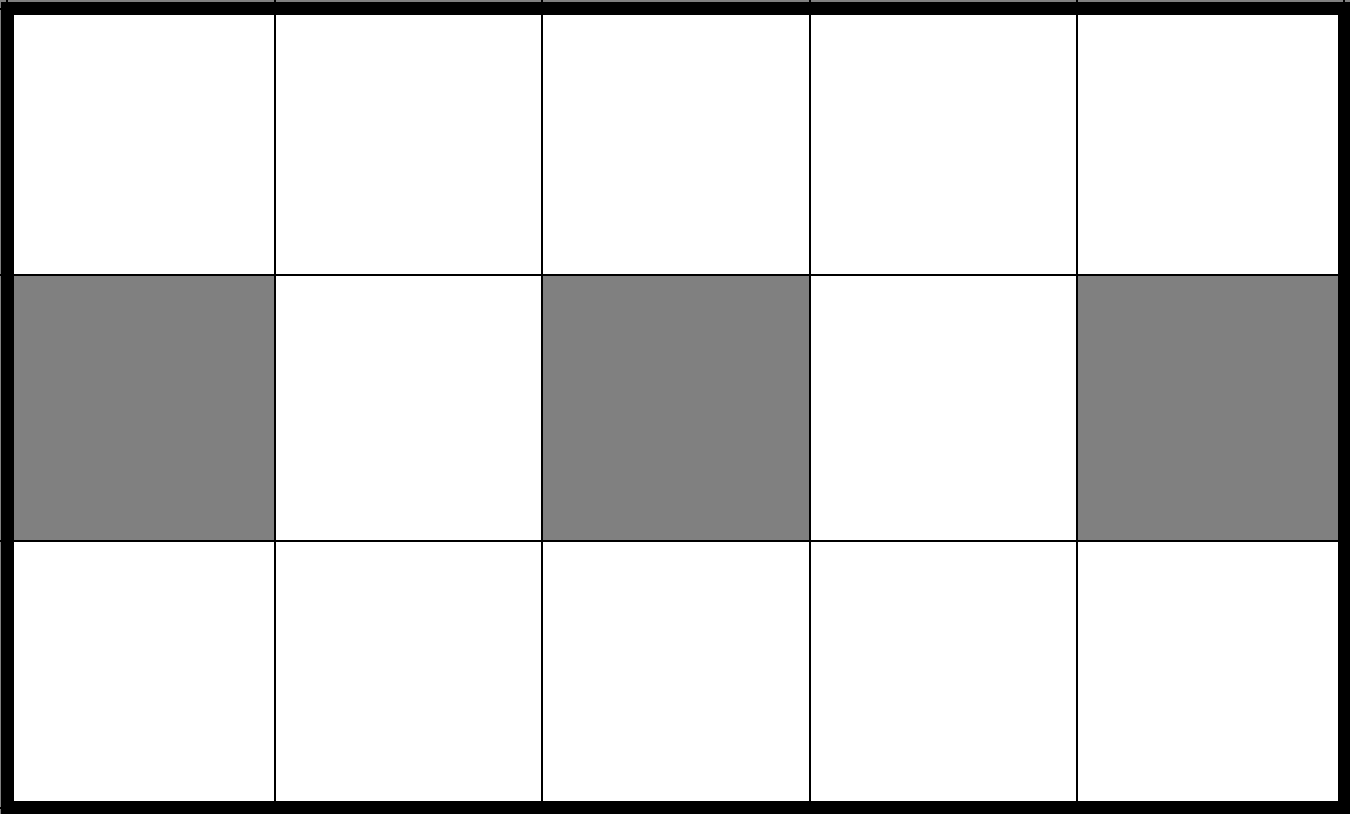
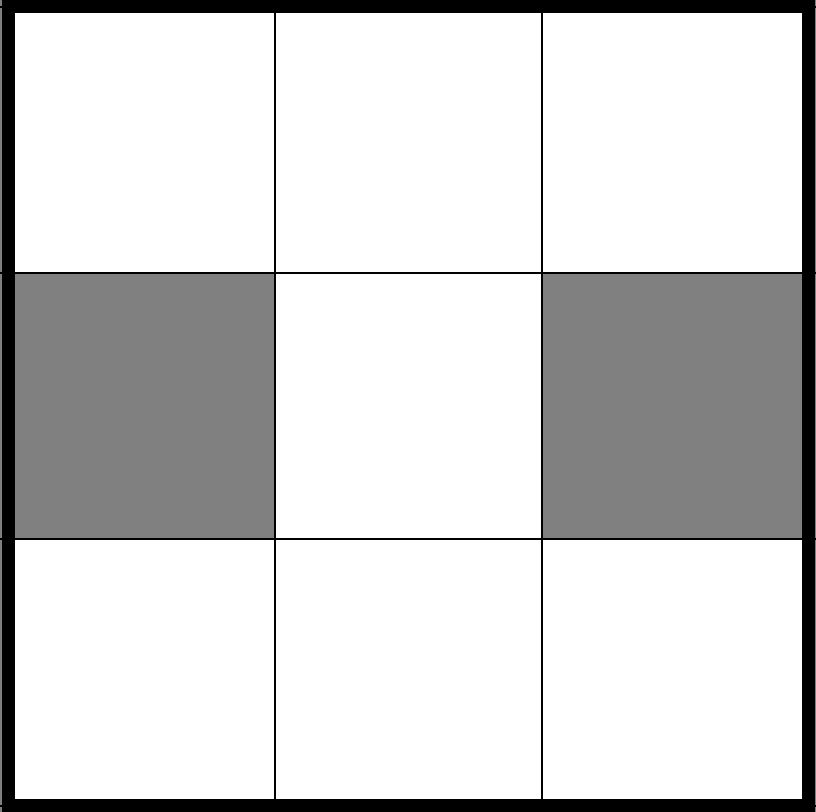
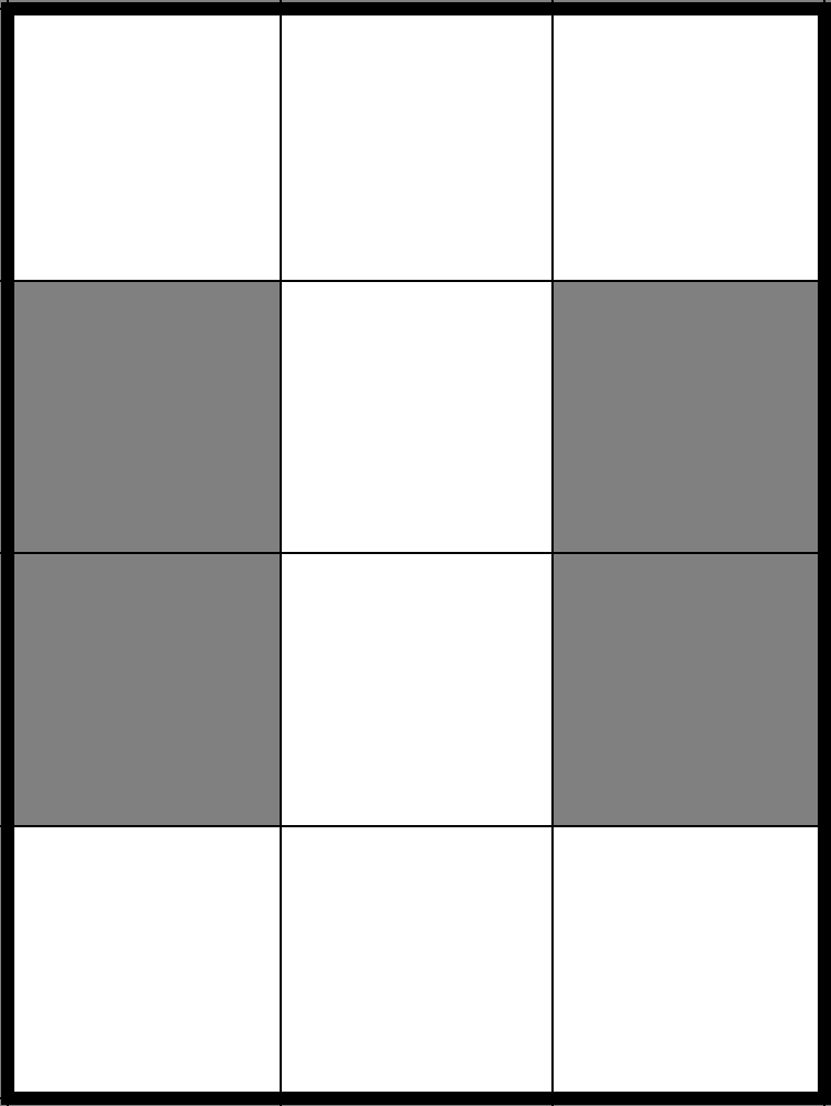
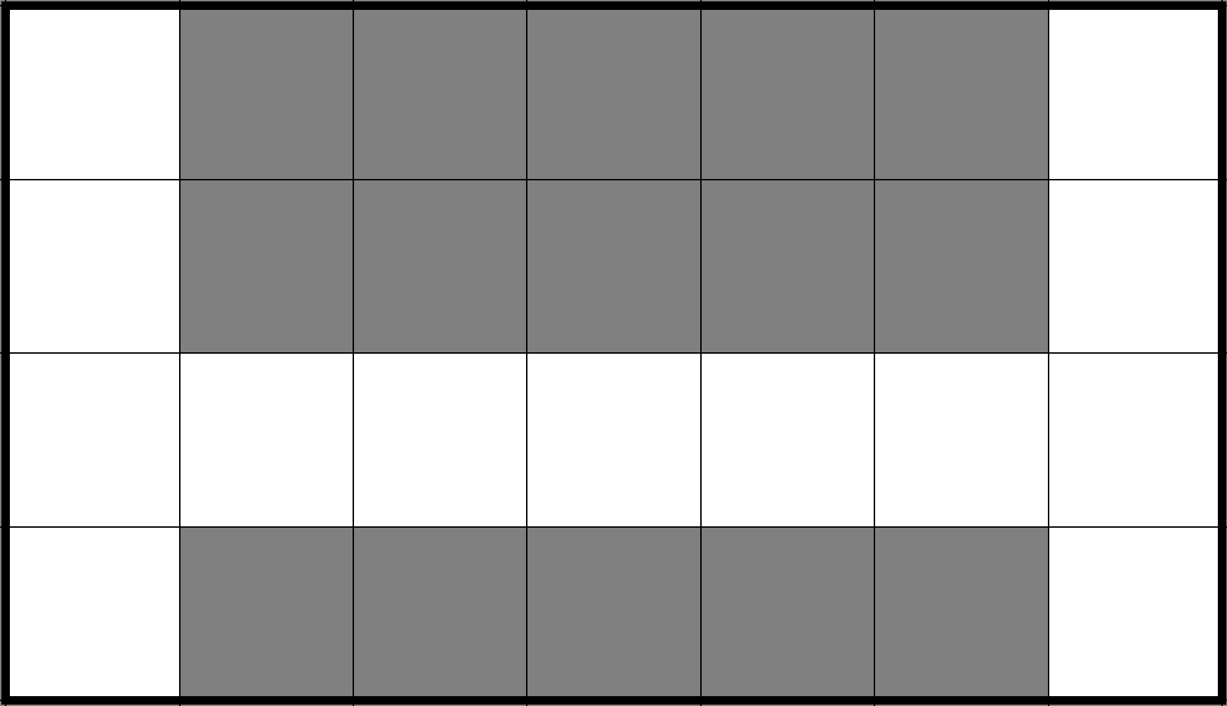
Figure 2: Manually designed layouts for the results reported in Table 2. From the left to the right, layouts are identified as id_1 to id_6.

To further investigate how the existence of feasible policies may depend on the capability of sensors, we first conduct experiments on six manually designed map layouts, as shown in Table 2. We evaluate the feasibility over all possible proper goal profiles for agents with sensors of different ranges. Detailed map layouts are shown in Figure 2. Map id_1 and id_2 are designed with roundabouts for two agent cases, and map id_3 – id_6 are designed to further include channels for three agent cases. Notice that except for map id_1 and id_4, agents need sensors of larger range to cover the whole map but actually sensors of range two already suffice. We additionally test the capability of sensor 1 versus sensor 2 under randomly generated maps in Table 3, where $4\times 4$ maps are associated with three agents and $5\times 5$ maps are associated with two agents. We report the number of profiles that allow feasible policies to exist, the number of proper profiles, as well as the total number of all randomly generated profiles. As one can see, in both Table 2 and Table 3, all profiles that cannot be solved by sensor 1 turn out to be solvable by sensor 2 with a success rate of 100%.

Map (#agents)	sensor 1	sensor 2	full sensor
#feasible/#total_proper
$\texttt{id\_1}(2)$	28/56	56/56	no need
$\texttt{id\_2}(2)$	46/56	56/56	56/56
$\texttt{id\_3}(3)$	0/168	168/168	168/168
$\texttt{id\_4}(3)$	0/24	24/24	no need
$\texttt{id\_5}(3)$	0/24	24/24	24/24
$\texttt{id\_6}(3)$	0/24	24/24	24/24

Table 2: Feasibilities with different sensors. For these manually designed layouts, see details in Figure 2.

Therefore, We highly conjecture that by excluding non-proper goal profiles, given any arbitrary map, if there is no policy for agents equipped with sensors of range two, then no feasible policy can be found for the same group of agents with sensors of range $i>2$.

Note that the converse is trivial, since the representational capability of sensors of larger range is always greater than that of sensors of smaller range. However, the above conjecture says that, sensors of range two will already suffice in terms of finding feasible policies. We try to (informally) justify the conjecture based on our observation from the above experiments and reasoning as follows.

1. If agents are only equipped with sensor 1, then they cannot effectively avoid vertex collision while they are two blocks away from each other yet cannot detect each other. Such coordination should be implicitly done by the centralized controller, which actually propagates more constraints to the program.

2. For two agent configurations, if both are equipped with sensor 2, informally speaking, one of them can always wait until she sees the other one and then they are allowed to coordinate in a completely observed sub-area.

3. However, when the number of agents is larger than two, as long as the sensor does not cover the whole map, there is always a case when $i$ can see $j$, $j$ can see $k$, but $k$ cannot see $i$. Since no communication is allowed in our settings, the existence of feasible policies in such situations is not obvious. However, according to our experiments in Table 2 and all $4\times 4$ layouts with three agents in Table 3, we have included such test cases and sensor 2 still suffices.

4. A more tricky case is about channels. If agents with sensor $i$ are placed under layouts with channels of length $l>2i$, there will be such cases when two are waiting at both entrances, one is already inside, but none of them is aware of the others. Our experiments on Map id_5 – id_6 have shown such test cases. If fact, for randomized $5\times 5$ layouts with two agents in Table 3, we have encountered more complex L-shaped channels and it turns out that sensor 2 still suffices.

5. The last possible case would be that there are so many agents that the map is too densely occupied, so that even if the goal profile is proper, there will still be no way for any sensor to work out feasible policies.

Map (#agents)	sensor 1	sensor 2
#feasible/#proper/#total
$4\times 4(3)$ 6% seed 1	61/63/100	63/63/100
$4\times 4(3)$ 6% seed 2	63/65/100	65/65/100
$4\times 4(3)$ 6% seed 3	63/68/100	68/68/100
$4\times 4(3)$ 12% seed 1	14/21/100	21/21/100
$4\times 4(3)$ 12% seed 2	61/63/100	63/63/100
$4\times 4(3)$ 12% seed 3	26/40/100	40/40/100
$4\times 4(3)$ 18% seed 1	40/45/100	45/45/100
$4\times 4(3)$ 18% seed 2	37/43/100	43/43/100
$4\times 4(3)$ 18% seed 3	13/29/100	29/29/100
$5\times 5(2)$ 10% seed 1	300/300/300	300/300/300
$5\times 5(2)$ 10% seed 2	268/268/300	268/268/300
$5\times 5(2)$ 10% seed 3	300/300/300	300/300/300
$5\times 5(2)$ 20% seed 1	163/163/300	163/163/300
$5\times 5(2)$ 20% seed 2	128/128/300	128/128/300
$5\times 5(2)$ 20% seed 3	238/300/300	300/300/300
$5\times 5(2)$ 30% seed 1	140/140/300	140/140/300
$5\times 5(2)$ 30% seed 2	145/145/300	145/145/300
$5\times 5(2)$ 30% seed 3	31/57/300	57/57/300

Table 3: For randomly generated maps, we randomize 300 goal profiles for $5\times 5$ layouts and 100 goal profiles for $4\times 4$ layouts. $4\times 4$ layouts are tested for three agents and $5\times 5$ layouts are tested for two agents. We set three density levels of obstacles 6%, 12%, and 18% for $4\times 4$ layouts, and 10%, 20%, and 30% for $5\times 5$ layouts. Three random seeds are experimented for each setting. Those layouts where sensor 2 is more capable than sensor 1 are marked in bold font. Sensor 2 in fact solves all profiles.

More evidence will be shown later in Table 4, where maps in larger size and even action restrictions are considered. As it turns out, even if we force agents to directly head towards their goals until when they have to coordinate to avoid collisions, sensors of range two are still capable enough of working out feasible policies.

5.2 Action Restrictions

Recall that a policy profile is a collection of individual policies $\pi_{i}:O_{i}\mapsto A$, and each individual policy is a mapping from the agent’s local states to available actions. When computing this mapping, it is sometime useful to partition the set of local states into disjoint subsets and make restrictions on what the mapping will need to satisfy according to different subsets. Here, for each agent $i$, we consider partitioning her local states into two subsets: $O_{i}=O_{i}^{+}\cup O_{i}^{-}$, where $O_{i}^{+}\cap O_{i}^{-}=\emptyset$, then computing a partial policy for each subset: $\pi_{i}^{+}:O_{i}^{+}\mapsto A$ and $\pi_{i}^{-}:O_{i}^{-}\mapsto A$, to get the full policy $\pi_{i}=\pi_{i}^{+}\cup\pi_{i}^{-}$. One can always attach some underlying meaning to the partition, e.g. $O_{i}^{-}$ can be the set of local states where agent $i$ does not detect any other agents. This will allow users to specify human-understandable preferences or restrictions on either part to make the computed policy fall into a desirable scope.

Action Preferences

In this subsection, we investigate the feasibility of policies under different semantics of $O_{i}^{-}$. To customize a preference ordering over actions, we associate each action with an integral cost under a given local state. Let the predicate cost(AS,A,C) define the Manhattan distance C from the local state AS to the goal by taking action A. The Manhattan distance is computed from the perspective of the agent herself, without any prescription of the actions that will be taken by other agents. Of course, any action that moves the agent into obstacles or beyond the map incurs an infinite cost. Note that several actions may tie with the same cost, i.e. the preference is not a strict one. Therefore agents who hold such preferences intend to make actions in a self-interested manner. We then ask the following questions, each for a real-world scenario:

1. Default action scenario: what if we impose such restrictions only when they do not see each other?

2. Last-minute coordination scenario: what if we impose such restrictions until when they are about to collide, if without appropriate coordination?

3. Myopic preference scenario: what if we impose such restrictions all along the way of routing?

For the above scenarios, from the top to the bottom, we actually assign a larger partition to $O_{i}^{-}$, and therefore impose stronger constraints on $\pi_{i}^{-}$. Intuitively, given empty maps, the least-Manhattan-distance action is the best most of the time, thus we can also evaluate the computed feasible policies by checking their sum-of-makespan to see how good they have already been, without particular optimization, for each of the three scenarios. First of all, we illustrate how to axiomatize them one by one.

For the first scenario, we modify the policy axiom as

{doi(AS,A):avai_action(AS,A)}=1 :-
    aState(AS), AS=(Self,Other,Goal),
    near(Self,Other), Other!=empty,
    Self!=Goal, goali(Goal).

{doi(AS,A): avai_action(AS,A),
    cost(AS,A,C0),
    cost(AS,up,C1), ..., cost(AS,nil,C5),
    C0<=C1,...,C0<=C5}=1 :-
    aState(AS), AS=(Self,empty,Goal),
    Self!=Goal, goali(Goal).

For the second scenario, we further sophisticate the policy axiom as

{doi(AS,A):avai_action(AS,A)}=1 :-
    aState(AS), AS=(Self,Other,Goal),
    near(Self,Other), Other!=empty,
    lastmin(Self,Other),
    Self!=Goal, goal2(Goal).

{doi(AS,A):avai_action(AS,A),
    cost(AS,A,C0),
    cost(AS,up,C1), ..., cost(AS,nil,C5),
    C0<=C1, ..., C0<=C5}=1 :-
    aState(AS), AS=(Self,Other,Goal),
    near(Self,Other), Other!=empty,
    not lastmin(Self,Other),
    Self!=Goal, goali(Goal).

{doi(AS,A):avai_action(AS,A),
    cost(AS,A,C0),
    cost(AS,up,C1), ..., cost(AS,nil,C5),
    C0<=C1, ..., C0<=C5}=1 :-
    aState(AS), AS=(Self,empty,Goal),
    Self!=Goal, goali(Goal).

where the lastmin predicate defines the moments when two agents are about to collide with each other if both make inappropriate actions.

lastmin(P1,P2):-
    P1=(X1,Y1), P2=(X2,Y2),
    cell(X1,Y1), cell(X2,Y2),
    |X1-X2|+|Y1-Y2|<=2.

For the third scenario, we do not have to discuss that many sub-cases, therefore, can simply write

{doi(AS,A):avai_action(AS,A),
    cost(AS,A,C0),
    cost(AS,up,C1), ..., cost(AS,nil,C5),
    C0<=C1, ..., C0<=C5}=1 :-
    aState(AS), AS=(Self,_,Goal),
    Self!=Goal, goali(Goal).

Scenario (map, #agents)	#Feasible	#Infeasible
Sensor 1
$\#1~{}(6\times 6,2)$	8/1260	1252/1260
Sensor 2
$\#1~{}(6\times 6,2)$	1260/1260	0/1260
$\#2~{}(6\times 6,2)$	1260/1260	0/1260
$\#3~{}(5\times 6,2)$	192/870	678/870
$\#3~{}(6\times 6,2)$	244/1260	1016/1260
$\#3~{}(6\times 7,2)$	300/1722	1422/1722
Sensor 3
$\#1~{}(6\times 6,2)$	1260/1260	0/1260
$\#2~{}(6\times 6,2)$	1260/1260	0/1260
$\#3~{}(5\times 6,2)$	192/870	678/870
$\#3~{}(6\times 6,2)$	244/1260	1016/1260
$\#3~{}(6\times 7,2)$	300/1722	1422/1722

Table 4: Feasible policies may or may not exist under certain restrictions. #1, #2, and #3 correspond to scenarios default action, last-minute coordination, and myopic preferences, respectively.

For a given map, we tested all possible goal profiles, e.g., $36\times 35=1260$ non-overlapping and proper goal profiles for a $6\times 6$ empty map with two agents. We report in Table 4 the number of profiles that allow feasible policies to exist. Notice that, even for the last-minute coordination scenario, sensors of range two allow feasible policies to exist for all goal profiles, which to some extent additionally verifies our conjecture in Section 5.1. We further elaborate on details for the third scenario in supplementary materials. Basically, a feasible policy exists in the myopic preference scenario as long as there is no “interior crossroads” formed by the goal profile.

As mentioned previously, it is also intriguing to investigate, without any optimization, how much the quality of a feasible policy can be improved only with the help of such action preferences. To this end, we evaluate the sum-of-makespan of the first feasible policy found by the ASP solver under different maps for each of the above restriction scenarios, respectively. One can clearly spot the large gap of improvement in Figure 3. An insightful conclusion would be that: given a general configuration, one may design certain single-agent heuristics over $O_{i}^{-}$ to polish the feasible policy, where $O_{i}^{-}$ does not span the whole $O_{i}$, i.e. agents are still allowed to coordinate themselves.

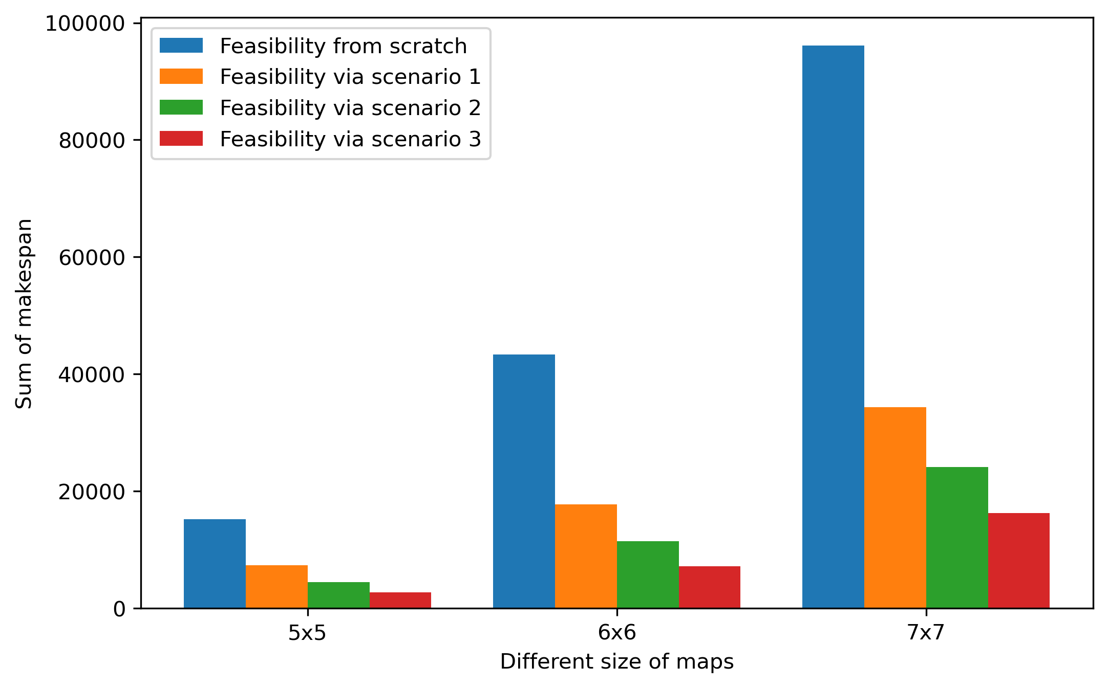
Figure 3: Sum-of-makespan evaluated on different maps with different restriction scenarios.

Traffic Rules

In addition to those single-agent restrictions imposed on $O_{i}^{-}$, we intend to find unified behavioral patterns, inspired by traffic systems, on $O_{i}^{+}$ by adding more axioms. When a driver is approaching traffic lights, her driving decisions are supposed to be made under certain traffic rules based on her relative observations of the other cars (i.e. whether the coming cars are on her left or right, instead of their GPS locations). Thus, a set of traffic rules is nothing but a common protocol that all drivers must obey and is viewed from the relative frame. In real-world situations, designers come up with certain rules first and then make all drivers aware of them. In this section, we investigate such an idea in a reversed manner by asking the question: making the whole system work, is there any possible traffic rule that is revealed?

Let $f:\bigcup_{i}O_{i}^{+}\mapsto O^{+}$ denote the function that transforms those local states where agents meet each other to a unified relative frame. A traffic rule is therefore a protocol $tr:O^{+}\mapsto A$ that maps those relative observations to available actions, and is known to all agents. Suppose the complementary policy $\pi_{i}^{-}:O_{i}^{-}\mapsto A$ can also be found, then the final policy profile can be collectively formed as $\{\pi_{i}\}_{i\in N}=\{\pi_{i}^{-}\cup(tr\circ f)\}_{i\in N}$.

As inspired by the real-world scenarios, there are two alternatives:

1. The traffic rule depends on the location of the agent and her relative observations of the others. (Different citys may impose different traffic rules.)

2. The traffic rule only depends the agent’s relative observations of the others no matter where she is. (In one single city, each crossroads is supposed to impose the same traffic rule.)

Scenario (map, agents)	#Found	#NotFound
Sensor 2
#1 $(6\times 6,2)$	1260/1260	0/1260
#1 $(6\times 6,2)$+default	1260/1260	0/1260
#2 $(6\times 6,2)$	0/1260	1260/1260
#2 $(6\times 6,2)$+default	0/1260	1260/1260
Sensor 3
#1 $(6\times 6,2)$	1260/1260	0/1260
#1 $(6\times 6,2)$+default	1260/1260	0/1260
#2 $(6\times 6,2)$	0/1260	1260/1260
#2 $(6\times 6,2)$+default	0/1260	1260/1260
Sensor 4
#1 $(6\times 6,2)$	1260/1260	0/1260
#1 $(6\times 6,2)$+default	1260/1260	0/1260
#2 $(6\times 6,2)$	0/1260	1260/1260
#2 $(6\times 6,2)$+default	0/1260	1260/1260
Sensor 5
#1 $(6\times 6,2)$	1260/1260	0/1260
#1 $(6\times 6,2)$+default	1260/1260	0/1260
#2 $(6\times 6,2)$	0/1260	1260/1260
#2 $(6\times 6,2)$+default	0/1260	1260/1260

Table 5: Certain traffic rule exist when it depends on agent’s locations, but no such traffic rule can be found if it is independent of agent’s locations. For both alternatives, we verify the existence for the naive version as well as the default action version.

Map (#agents)	from scratch			default action			last-minute coordination
	start	end	improve	start	end	improve	start	end	improve
Sensor 2
$3\times 3$ (2)	360	181	49.72%	415	263	36.63%	264	203	23.11%
$4\times 4$ (2)	4298	2732	36.44%	2653	2473	6.78%	1250	1241	0.72%
$5\times 5$ (2)	15248	15149	0.65%	7349	7302	0.64%	4436	4422	0.32%
$6\times 6$ (2)	43355	41007	5.42%	17734	17331	2.27%	11420	11420	0.00%
Sensor 3
$4\times 4$ (2)	3391	3379	0.35%	3368	3256	3.33%	1462	1441	1.44%
$5\times 5$ (2)	14962	14746	1.44%	10423	10105	3.05%	4605	4539	11.43%
$6\times 6$ (2)	52530	45953	12.52%	26873	26873	0.00%	11544	11526	0.16%
Sensor 4
$5\times 5$ (2)	22801	21950	3.73%	14359	11277	21.46%	4894	4882	0.25%
$6\times 6$ (2)	54669	48316	11.62%	29242	29238	0.01%	11669	11628	0.35%

Table 6: Optimization procedures starting from different action restrictions. The subtitle “start” means the sum-of-makespan of first feasible policy while “end” means that of the last one, after which no better one has been found for 2 hours. “Default action” and “last-minute coordination” correspond to respective restriction scenarios in Section 5.2.

For the first alternative, the policy axioms for $\pi_{i}^{+}$ are modified as follows.

{traffic(Self,Rel_pos,A):
    avai_action(AS,A)}=1 :-
    aState(AS), AS=(Self,Other,Goal),
    near(Self,Other), Other!=empty,
    Self=(X1,Y1), Other=(X2,Y2),
    Rel_pos=(X2-X1,Y2-Y1),
    Self != Goal.

{doi(AS,A):
    traffic(Self,Rel_pos,A)}=1 :-
    aState(AS), AS=(Self,Other,Goal),
    near(Self,Other), Other!=empty,
    Self=(X1,Y1), Other=(X2,Y2),
    Rel_pos=(X2-X1,Y2-Y1),
    Self!=Goal, goali(Goal).

Note that we omit the axiom for $\pi_{i}^{-}$ here. One can opt to impose the default action restriction on those local states where agents detect no one else. If so, then both agents are actually adopting the same strategy (but not the same policy) when they have not met each other, and then enquire the same protocol when they meet. As shown in Table 5, even default actions are preferred, one can always find certain traffic rules only with the help of sensors of range two.

For the second alternative, we instead include the following axioms.

{traffic(Rel_pos,A):
    avai_action(AS,A)}=1 :-
    aState(AS), AS=(Self,Other,Goal),
    near(Self,Other), Other!=empty,
    Self=(X1,Y1), Other=(X2,Y2),
    Rel_pos=(X2-X1,Y2-Y1),
    Self!=Goal.

{doi(AS,A):
    traffic(Rel_pos,A)}=1 :-
    aState(AS), AS=(Self,Other,Goal),
    near(Self,Other), Other!=empty,
    Self=(X1,Y1), Other=(X2,Y2),
    Rel_pos=(X2-X1,Y2-Y1),
    Self!=Goal, goali(Goal).

And also, one can implement $\pi_{i}^{-}$ as the default action version. As shown in Table 5, no such traffic rule is found even if we does not force agents to follow default actions yet equip them with the most powerful sensors of range five which already cover the whole $6\times 6$ map. One reasonable explanation is: unlike real-world traffic systems, our artificial map is bounded, agents are supposed to behave differently while they are approaching the boundary, instead of doing the same as in the interior places of the map.

5.3 Anytime Optimization

As mentioned before, one can always divide the policy twofold. When it comes to policy optimization, the system designer can also firstly specify human-understandable strategies ahead of time for $\pi_{i}^{-}$. The planning and optimization procedures are therefore only responsible for (optimally) “completing” the rest $\pi_{i}^{+}$. In our settings, we have designed several action preferences for specifying $\pi_{i}^{-}$ in Section 5.2. As reported in Table 6, we experiment on starting optimizing the policy from different action restrictions as well as from scratch. The program is terminated after a long enough period with no better solutions found. It shows that the improvement gained from optimization is much less than that gained by adding good constraints. A lesson taken from this table is that, to have better policies, attention should be paid to figuring out helpful constraints or properties that (near-)optimal policies are compatible with, instead of leaving the work to existing optimization tools.

6 Conclusion

In this paper, we implement the system ASP-MAUPF for computing policies for any arbitrary map and a group of partially observable agents with dedicated goals. The system is utilized for comprehensive studies of the behavioral patterns of agents. With the help of ASP, we are able to easily axiomatize user-specified preferences, and therefore polish the policy.

Furthermore, we point out several potential directions or applications of our system.

• Despite the fact that compared to existing Dec-POMDP solvers, we can solve larger problem instances, real-world applications such as warehouse automation and logistics require solvers that can scale to huge maps and even swarms of robots, which are intractable for our system yet. One possible way is to leverage our system to compute policies for (local) multi-agent coordination in sub-regions and single-agent planners to guide agents while they are walking alone.

• Another useful application is to embed our rule-based system into a learning framework. Similarly, acceleration rules and safety rules are manually designed for single-agent RL tasks (?). However, our system sheds light on how to automate the generation of rules to assist learning even in multi-agent domains.

References

- Amato, Bernstein, and Zilberstein 2010 Amato, C.; Bernstein, D. S.; and Zilberstein, S. 2010. Optimizing fixed-size stochastic controllers for pomdps and decentralized pomdps. Autonomous Agents and Multi-Agent Systems 21:293–320.
- Belov et al. 2020 Belov, G.; Du, W.; De La Banda, M. G.; Harabor, D.; Koenig, S.; and Wei, X. 2020. From multi-agent pathfinding to 3d pipe routing. In Proceedings of the International Symposium on Combinatorial Search, volume 11, 11–19.
- Bernstein et al. 2009 Bernstein, D. S.; Amato, C.; Hansen, E. A.; and Zilberstein, S. 2009. Policy iteration for decentralized control of markov decision processes. Journal of Artificial Intelligence Research 34:89–132.
- Bogatarkan and Erdem 2020 Bogatarkan, A., and Erdem, E. 2020. Explanation generation for multi-modal multi-agent path finding with optimal resource utilization using answer set programming. Theory and Practice of Logic Programming 20(6):974–989.
- Bogatarkan, Patoglu, and Erdem 2019 Bogatarkan, A.; Patoglu, V.; and Erdem, E. 2019. A declarative method for dynamic multi-agent path finding. In GCAI, 54–67.
- Bonet and Geffner 2011 Bonet, B., and Geffner, H. 2011. Planning under partial observability by classical replanning: Theory and experiments. In Twenty-Second International Joint Conference on Artificial Intelligence.
- Chen et al. 2022 Chen, Z.; Li, J.; Harabor, D.; Stuckey, P. J.; and Koenig, S. 2022. Multi-train path finding revisited. In Proceedings of the Symposium on Combinatorial Search (SoCS), 38–46.
- Foerster et al. 2018 Foerster, J.; Farquhar, G.; Afouras, T.; Nardelli, N.; and Whiteson, S. 2018. Counterfactual multi-agent policy gradients. In Proceedings of the AAAI conference on artificial intelligence, volume 32.
- Gao et al. 2020 Gao, Z.; Lin, F.; Zhou, Y.; Zhang, H.; Wu, K.; and Zhang, H. 2020. Embedding high-level knowledge into dqns to learn faster and more safely. In Proceedings of the AAAI Conference on Artificial Intelligence, volume 34, 13608–13609.
- Gebser et al. 2011 Gebser, M.; Kaufmann, B.; Kaminski, R.; Ostrowski, M.; Schaub, T.; and Schneider, M. 2011. Potassco: The potsdam answer set solving collection. Ai Communications 24(2):107–124.
- Gebser et al. 2019 Gebser, M.; Kaminski, R.; Kaufmann, B.; and Schaub, T. 2019. Multi-shot asp solving with clingo. Theory and Practice of Logic Programming 19(1):27–82.
- Gómez, Hernández, and Baier 2020 Gómez, R. N.; Hernández, C.; and Baier, J. A. 2020. Solving sum-of-costs multi-agent pathfinding with answer-set programming. In Proceedings of the AAAI Conference on Artificial Intelligence, volume 34, 9867–9874.
- Kaelbling, Littman, and Cassandra 1998 Kaelbling, L. P.; Littman, M. L.; and Cassandra, A. R. 1998. Planning and acting in partially observable stochastic domains. Artificial intelligence 101(1-2):99–134.
- Li et al. 2019a Li, J.; Surynek, P.; Felner, A.; Ma, H.; Kumar, T. K. S.; and Koenig, S. 2019a. Multi-agent path finding for large agents. In Proceedings of the AAAI Conference on Artificial Intelligence (AAAI), 7627–7634.
- Li et al. 2019b Li, J.; Zhang, H.; Gong, M.; Liang, Z.; Liu, W.; Tong, Z.; Yi, L.; Morris, R.; Pasareanu, C.; and Koenig, S. 2019b. Scheduling and airport taxiway path planning under uncertainty. In Proceedings of the AIAA Aviation Forum.
- Li et al. 2021 Li, J.; Chen, Z.; Zheng, Y.; Chan, S.-H.; Harabor, D.; Stuckey, P. J.; Ma, H.; and Koenig, S. 2021. Scalable rail planning and replanning: Winning the 2020 flatland challenge. In Proceedings of the International Conference on Automated Planning and Scheduling (ICAPS), 477–485.
- Littman 2009 Littman, M. L. 2009. A tutorial on partially observable markov decision processes. Journal of Mathematical Psychology 53(3):119–125.
- Lowe et al. 2017 Lowe, R.; Wu, Y. I.; Tamar, A.; Harb, J.; Pieter Abbeel, O.; and Mordatch, I. 2017. Multi-agent actor-critic for mixed cooperative-competitive environments. Advances in neural information processing systems 30.
- Madani, Hanks, and Condon 1999 Madani, O.; Hanks, S.; and Condon, A. 1999. On the undecidability of probabilistic planning and infinite-horizon partially observable markov decision problems. In AAAI/IAAI, 541–548. Citeseer.
- Oliehoek and Amato 2016 Oliehoek, F. A., and Amato, C. 2016. A concise introduction to decentralized POMDPs. Springer.
- Rendsvig and Symons 2021 Rendsvig, R., and Symons, J. 2021. Epistemic Logic. In Zalta, E. N., ed., The Stanford Encyclopedia of Philosophy. Metaphysics Research Lab, Stanford University, Summer 2021 edition.
- Sartoretti et al. 2019 Sartoretti, G.; Kerr, J.; Shi, Y.; Wagner, G.; Kumar, T. S.; Koenig, S.; and Choset, H. 2019. Primal: Pathfinding via reinforcement and imitation multi-agent learning. IEEE Robotics and Automation Letters 4(3):2378–2385.
- Schoppers 1987 Schoppers, M. 1987. Universal plans for reactive robots in unpredictable environments. In IJCAI, volume 87, 1039–1046. Citeseer.
- Sharon et al. 2015 Sharon, G.; Stern, R.; Felner, A.; and Sturtevant, N. R. 2015. Conflict-based search for optimal multi-agent pathfinding. Artificial Intelligence 219:40–66.
- Stern et al. 2019 Stern, R.; Sturtevant, N. R.; Felner, A.; Koenig, S.; Ma, H.; Walker, T. T.; Li, J.; Atzmon, D.; Cohen, L.; Kumar, T. S.; et al. 2019. Multi-agent pathfinding: Definitions, variants, and benchmarks. In Twelfth Annual Symposium on Combinatorial Search.
- Stern 2019 Stern, R. 2019. Multi-agent path finding–an overview. Artificial Intelligence 96–115.
- Surynek et al. 2016 Surynek, P.; Felner, A.; Stern, R.; and Boyarski, E. 2016. Efficient sat approach to multi-agent path finding under the sum of costs objective. In Proceedings of the twenty-second european conference on artificial intelligence, 810–818.
- Surynek 2019 Surynek, P. 2019. Unifying search-based and compilation-based approaches to multi-agent path finding through satisfiability modulo theories. In Proceedings of the 28th International Joint Conference on Artificial Intelligence, 1177–1183.
- Tran et al. 2023 Tran, S. C.; Pontelli, E.; Balduccini, M.; and Schaub, T. 2023. Answer set planning: A survey. Theory and Practice of Logic Programming 23(1):226–298.
- Varambally, Li, and Koenig 2022 Varambally, S.; Li, J.; and Koenig, S. 2022. Which MAPF model works best for automated warehousing? In Proceedings of the Symposium on Combinatorial Search (SoCS), 190–198.
- Wang et al. 2019 Wang, J.; Li, J.; Ma, H.; Koenig, S.; and Kumar, S. 2019. A new constraint satisfaction perspective on multi-agent path finding: Preliminary results. In 18th International Conference on Autonomous Agents and Multi-Agent Systems.
- Yalciner et al. 2017 Yalciner, I. F.; Nouman, A.; Patoglu, V.; and Erdem, E. 2017. Hybrid conditional planning using answer set programming. Theory and Practice of Logic Programming 17(5-6):1027–1047.
- Yu and LaValle 2013 Yu, J., and LaValle, S. M. 2013. Structure and intractability of optimal multi-robot path planning on graphs. In Twenty-Seventh AAAI Conference on Artificial Intelligence.
- Zanuttini et al. 2020 Zanuttini, B.; Lang, J.; Saffidine, A.; and Schwarzentruber, F. 2020. Knowledge-based programs as succinct policies for partially observable domains. Artificial Intelligence 288:103365.