MaskCL: Semantic Mask-Driven Contrastive Learning for Unsupervised clothes-change Person Re-Identification

MaskCL: Semantic Mask-Driven Contrastive Learning for Unsupervised Person Re-Identification with Clothes Change

Abstract

This paper considers a novel and challenging problem: unsupervised long-term person re-identification with clothes change. Unfortunately, conventional unsupervised person re-id methods are designed for short-term cases and thus fail to perceive clothes-independent patterns due to simply being driven by RGB prompt. To tackle with such a bottleneck, we propose a semantic mask-driven contrastive learning approach, in which silhouette masks are embedded into contrastive learning framework as the semantic prompts and cross-clothes invariance is learnt from hierarchically semantic neighbor structure by combining both RGB and semantic features in a two-branches network. Since such a challenging re-id task setting is investigated for the first time, we conducted extensive experiments to evaluate the state-of-the-art unsupervised short-term person re-id methods on five widely-used clothes-change re-id datasets. Experimental results verify that our approach outperforms the unsupervised re-id competitors by a clear margin, remaining a narrow gap to the supervised baselines.

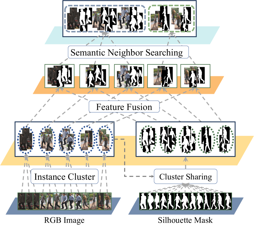
Figure 1: Illustration of hierarchical semantic clustering. At a lower level, clustering is used to disclose the instance neighbor structure; at a higher level, semantic features and RGB data are combined to expose the cluster neighbor structure.

1 Introduction

Person re-identification (re-id) aims to match person identities of bounding box images that are captured from distributed camera views [51]. Most conventional studies in the field of unsupervised person re-id have only focused on the scenarios without clothes change [53, 47, 11]. However, re-id in such scenarios is unrealistic since that the majority of people may change their clothing everyday, if not more often. Thus, these studies may only be useful in the short-term re-id settings but fail when facing the long-term person re-id scenario with clothes changes.

Recently, there are a few attempts to tackle with the long-term re-id task [49, 18, 45, 15], but all of them are supervised learning methods with heavy reliance on large labeled training data. Unfortunately, it is extremely difficult to collect and annotate the person identity labels under the scenario of unconstrained clothes change, thus preparing the labeled re-id training data, e.g., Deepchange [48], in a realistic scenario is quite expensive and exhausting.

Due to the significance of long-term person re-id, it is appealing to develop unsupervised method to approach long term person re-id problem without the tedious requirement of person identity labeling. This is a more complex but more realistic extension of the previous unsupervised short-term person re-id [30, 12, 29] that different people may have similar clothes whilst the same person might wear variant clothes with very distinct appearances, as shown in Figure 2. Unfortunately, previous studies of unsupervised person re-id have not dealt with the clothes change cases and existing methods will fail to perceive clothes-independent patterns due to simply being driven by RGB prompts [28]. Specifically, most of the existing unsupervised methods [8] are cluster-based and the feature extractions are mostly dominated by color [28]. As a consequence, the clustering algorithm will blindly assign every training sample with a color-based pseudo label, which is error-prone with a large cumulative propagation risk and ultimately leads to sub-optimal solutions, such as simply grouping the individuals who wear the same clothing.

In this paper, we propose a novel semantic mask-driven contrastive learning framework, termed MaskCL, for attacking the unsupervised long-term person re-id challenge. In MaskCL, we embed the person silhouette mask as the semantic prompts into contrastive learning framework and learn cross-clothes invariance features of pedestrian images from a hierarchical semantic neighbor structure with a two-branches network. Specifically, MaskCL adopts a contrast learning framework to mine the invariance between semantic silhouette masks and RGB images to further assist the network in learning clothes-irrelevant features. In the contrastive training stage, we employ RGB features to generate clusters, thus images of individuals wearing the same clothes tend to be clustered together owing to their greater resemblance. At the meantime, since that silhouette masks contain rich clothes-invariant features, we use it as semantic prompts to combine with features from RGB images to unveil the hidden neighbor structure at the cluster level. Consequently, we fuse the clustering result (based on RGB features) and semantic neighbor sets (based on semantic prompts) to form a hierarchical neighbor structure and use it to drive model training for reducing feature disparities due to clothes change.

To provide a comprehensive evaluation and comparison, we evaluate recent unsupervised person re-id methods on five long-term person re-id datasets. Experimental results demonstrate that our approach significantly outperforms all short-term methods and even matches the the state-of-the-art fully supervised models on these datasets.

The contributions of the paper are highlighted as follows.

1. To the best of our knowledge, this is the first attempt to study the unsupervised long-term person re-id with clothes change.

2. We present a hierarchically semantic mask-based contrastive learning framework, in which person silhouette masks are used as semantic prompt and a hierarchically semantic neighbor structure is constructed to learn cross-clothes invariance.

3. We conduct extensive experiments on five widely-used clothes-change re-id datasets to evaluate the performance of the proposed approach. These evaluation results can serve as a benchmarking ecosystem for the long-term person re-id community.

Figure 2: Visualizing the intrinsic challenges in long-term person re-id with clothes change. We randomly selected $28$ images of a single individual from the Deepchange [48] dataset. It is clear that the differences in appearance across different clothes (rows) are much more significant than that of the same clothes (each column).

2 Related Work

2.1 Long-Term Person Re-Identification

A few recent person re-id studies attempt to tackle [49, 18, 36, 33, 41, 46, 45] the long-term clothes changing situations via supervised training, and emphasize the use of additional supervision for the general appearance features (e.g., clothes, color), to enable the model learn the cross-clothes features. For example, Yang et al. [49] generates contour sketch images from RGB images and highlights the invariance between sketch and RGB. Hong et al. [15] explore fine-grained body shape features by estimating masks with discriminative shape details and extracting pose-specific features. While these seminal works provide inspiring attempts for re-id with clothes change, there are still some limitations: a) Generating contour sketches or other side-information requires additional model components and will cause extra computational cost; b) To the best of our knowledge, all the existing models designed for re-id clothes change are supervised learning methods, with lower transferability to the open-world dataset settings. In this paper, we attempt to tackle with the challenging re-id with clothes change under unsupervised setting.

2.2 Unsupervised Person Re-Identification

To meet the increasing demand in real life and to avoid the high consumption in data labelling, a large and growing body of literature has investigated unsupervised person re-id [54, 34, 44]. The existing unsupervised person Re-ID methods can be divided into two categories: a) unsupervised domain adaptation methods, which require a labeled source dataset and an unlabelled target dataset [34, 1, 35, 44]; and b) purely unsupervised methods that work with only an unlabelled dataset [28, 6, 3, 8]. However, up to date, the unsupervised person re-id methods are focusing on short-term scenarios, none of them taking into account the long-term re-id scenario. To the best of our knowledge, this is the first attempt to address the long-term person re-id in unsupervised setting. We evaluate the performance of the existing the state-of-the-art unsupervised methods [12, 28, 8, 29, 6, 3] on five long-term person re-id datasets and set up a preliminary benchmarking ecosystem for the long-term person re-id community.

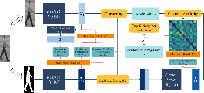
Figure 3: Illustration for our proposed Semantic Mask-driven Contrastive Learning (MaskCL) framework.

3 Our Proposed Approach: Semantic Mask-driven Contrastive Learning (MaskCL)

This section presents a semantic mask-driven contrastive learning (MaskCL) approach for unsupervised long-term person re-id with clothes change.

For clarity, we provide the flowchart of MaskCL in Fig. 3. Our MaskCL is a two branches network: $F(\cdot|\Theta)$ and $F^{\prime}(\cdot|\Theta^{\prime})$, which perceive RGB and semantic mask patterns, respectively, and $\Theta$ and $\Theta^{\prime}$ denote the parameters in the networks. The parameters $\Theta$ and $\Theta^{\prime}$ are optimized separately. We also design a predictor layer $G(\cdot|\Psi)$ where $\Psi$ denotes the parameters subsequent to RGB branch. In addition, we design a feature fusion layer $R(\cdot|\Omega)$, where $\Omega$ denotes the parameters.

Given an unlabeled pedestrian image dataset $\mathcal{I}={\{I_{i}}\}_{i=1}^{N}$ consisting of $N$ samples, we generate the corresponding pedestrian semantic mask dataset $\mathcal{S}={\{S_{i}}\}_{i=1}^{N}$ through human parsing network such as SCHP [31]. For an input image $I_{i}\in\mathcal{I}$, we use the $I_{i}$ as the input of $F(\cdot|\Theta)$ and $S_{i}$ as the inputs of $F^{\prime}(\cdot|\Theta^{\prime})$. For simplicity, we denote the output features of the $F(\cdot|\Theta)$ and $F^{\prime}(\cdot|\Theta^{\prime})$ as $\boldsymbol{x}_{i}$ and $\tilde{\boldsymbol{x}}_{i}$, denote the output of the predictor layer in the $G(\cdot|\Psi)$ as $\boldsymbol{z}_{i}$, and denote the output of fusion layer $R(\cdot|\Omega)$ as $\boldsymbol{f}_{i}$, respectively, where $\boldsymbol{x}_{i},\tilde{\boldsymbol{x}}_{i},\boldsymbol{z}_{i},\boldsymbol{f}_{i}\in\mathbb{R}^{D}$.

The training of MaskCL alternates between representation learning and hierarchical semantic structure construction. In hierarchical semantic structure creation, the hierarchical semantic neighbor structure is constructed by integrating RGB and semantic data to drive the training of the contrast learning framework, the details are described in Section 3.1. In feature learning, we introduce the person’s silhouette masks as the semantic source and investigate cross-clothes features via contrastive learning. In the training phase, MaskCL uses the hierarchical semantic neighbor structure as self-supervision information to train the $F(\cdot|\Theta)$, $F^{\prime}(\cdot|\Theta^{\prime})$, $G(\cdot|\Psi)$ and $R(\cdot|\Omega)$. The details are described in Section 3.2. Furthermore, we build an adaptive learning strategy to automatically modify the hierarchical semantic neighbor selection, which can flexibly select neighbor clusters according to dynamic criteria. The details are described in Section 3.3.

In MaskCL, we maintain the three instance-memory banks $\mathcal{M}=\{\boldsymbol{v}_{i}\}_{i=1}^{N}$, $\tilde{\mathcal{M}}=\{\boldsymbol{\tilde{v}}_{i}\}_{i=1}^{N}$, and $\hat{\mathcal{M}}=\{\boldsymbol{\hat{v}}_{i}\}_{i=1}^{N}$, where $\boldsymbol{v}_{i},\boldsymbol{\tilde{v}}_{i},\boldsymbol{\hat{v}}_{i}\in\mathbb{R}^{D}$ to store the outputs of the two branches and the fusion layer, respectively. Memory banks $\mathcal{M}$ and $\hat{\mathcal{M}}$ are initialized with $\mathcal{X}:=\{\boldsymbol{x}_{1},\cdots,\boldsymbol{x}_{N}\}$ and $\tilde{\mathcal{M}}$ is initialized with $\tilde{\mathcal{X}}:=\{\tilde{\boldsymbol{x}}_{1},\cdots,\tilde{\boldsymbol{x}}_{N}\}$, where $\mathcal{X}$ and $\tilde{\mathcal{X}}$ are the outputs of the network branches $F(\cdot|\Theta)$ and $F^{\prime}(\cdot|\Theta^{\prime})$ pre-trained on ImageNet, respectively.

3.1 Hierarchical Semantic Clustering

To have a hierarchical semantic clustering, we sort the hierarchical semantic structure into two levels: a) low-level instance neighbors, and b) high-level semantic neighbors.

Low-level instance neighbors. At beginning, we pre-train the two network branches $F(\cdot|\Theta)$ and $F^{\prime}(\cdot|\Theta^{\prime})$ on ImageNet [27], and use the branch $F(\cdot|\Theta)$ outputs features to yield $m$ clusters, which are denoted as $\mathcal{C}:=\{\mathcal{C}^{(1)},\mathcal{C}^{(2)},\cdots,\mathcal{C}^{(m)}\}$. We use the clustering results $\mathcal{C}$ to indicate the connection between neighbors at the instance level since that if samples are clustered together, it also indicates that their RGB features are similar.

High-level semantic neighbors. Since that the semantic masks contain richer clothing invariance features, we use them to find those pedestrian samples that are similar at the semantic level, e.g., the same person wearing different clothing. To be specific, we fuse the RGB feature and the semantic feature to renew the representation of instance, and search the semantic neighbor at the cluster-level based on fusion features. For an image $\mathbf{I}_{i}$, the fusion feature $\boldsymbol{f}_{i}$ is defined as:

$$\boldsymbol{f}_{i}=F(concate(\boldsymbol{x}_{i}|\tilde{\boldsymbol{x}}_{i})),$$ (1)

where $concate(\cdot)$ denotes the operation of concatenating feature $\boldsymbol{x}_{i}$ and $\tilde{\boldsymbol{x}}_{i}$ at channel-wise. Based on the fused features, we define the cluster center $\boldsymbol{u}_{\omega(\mathbf{I}_{i})}$ accordingly as follows:

$$\boldsymbol{u}_{\omega(\mathbf{I}_{i})}=\frac{1}{|\mathcal{C}^{(\omega(\mathbf{I}_{i}))}|}\sum_{I_{j}\in\mathcal{C}^{(\omega(\mathbf{I}_{i}))}}\boldsymbol{f}_{j},$$ (2)

where $\omega(\mathbf{I}_{i})$ is the cluster index of image $\mathbf{I}_{i}$.

Having had cluster-center $\boldsymbol{U}={\{\boldsymbol{u_{i}}}\}_{i=1}^{m}$, we find cluster-level semantic neighbors and construct the semantic neighbor set $\mathcal{N}$. Specifically, for cluster $\mathcal{C}^{(\ell)}$, we define the similarity between clusters $\mathcal{C}^{(\ell)}$ and $\mathcal{C}^{(i)}$ as

$$\mathcal{D}(\mathcal{C}^{(\ell)},\mathcal{C}^{(i)})=\frac{\boldsymbol{u}_{\ell}^{\top}}{\|\boldsymbol{u}_{\ell}\|_{2}}\frac{\boldsymbol{u}_{i}}{\|\boldsymbol{u}_{i}\|_{2}}.$$ (3)

We denote the semantic neighbor set of cluster $\mathcal{C}^{(\ell)}$ as $\mathcal{N}^{(\ell)}$, which includes the top-$k$ similar clusters $\mathcal{C}^{(i)}$ sorted by $\mathcal{D}(\mathcal{C}^{(\ell)},\mathcal{C}^{(i)})$. Then, we form a semantic neighbor set $\mathcal{A}:=\{\mathcal{N}^{(1)},\cdots,\mathcal{N}^{(m)}\}$. Because of the hierarchy property to define the set class $\mathcal{A}$, we call the process as the hierarchical semantic clustering.

In the hierarchical semantic clustering stage, we construct neighbor structures based on some specific clustering algorithm and semantic neighbor searching, respectively. The clustering result of the output features $\mathcal{X}:=\{\boldsymbol{x}_{1},\cdots,\boldsymbol{x}_{N}\}$ from $F(\cdot|\Theta)$ is used to generate the pseudo labels $\mathcal{Y}:=\{\boldsymbol{y}_{1},\cdots,\boldsymbol{y}_{N}\}$, and semantic neighbor set $\mathcal{A}$ contains the semantic level neighbor index for each cluster. In the contrastive learning stage, both the clustering result and the semantic neighbor set are used as self-supervision information to train the model to learn cross-clothes features.

3.2 Contrastive Learning Framework

To effectively explore the invariance features between RGB images and semantic masks, we construct three contrastive learning modules to train MaskCL assisted with the self-supervision information provided by the hierarchical semantic clustering as follows: a) Prototypical contrastive learning module, which is used for contrast training between positive samples and negative pairs; b) Cross-view contrastive learning module, which is used for contrast training between RGB images and semantic masks; and c) Semantic neighbor contrastive learning module, which is used for contrast training between semantic neighbor clusters and negative pairs.

Prototypical Contrastive Learning Module. We apply prototypical contrastive learning to discover the hidden information inside the cluster structure. For the $i$-th instance, we denote its cluster index as $\omega(I_{i})$, the center of $C^{\omega(I_{i})}$ as the positive prototype, and all other cluster centers as the negative prototypes. We define the prototypical contrastive learning loss as follows:

$$\mathcal{L}_{P}= -((1-q_{i})^{2}\ln(q_{i})$$ (4)

$$+(1-\tilde{q}_{i})^{2}\ln(\tilde{q}_{i})+(1-\hat{q}_{i})^{2}\ln(\hat{q}_{i})),$$

where $q_{i}$, $\tilde{q}_{i}$ and $\hat{q}_{i}$ measure the consistency between the outputs of $F(\cdot|\Theta)$, $F^{\prime}(\cdot|\Theta^{\prime})$ and $R(\cdot|\Omega)$ and the related prototype computed with the memory bank and are defined as

$$q_{i}=\frac{\exp(p_{{\omega(I_{i})}}^{\top}{\boldsymbol{x}_{i}}/\tau)}{\sum_{\ell=1}^{m}\exp(p_{\ell}^{\top}{\boldsymbol{x}_{i}}/\tau)},$$ (5)

$$\tilde{q}_{i}=\frac{\exp(\tilde{p}_{{\omega(I_{i})}}^{\top}{\tilde{\boldsymbol{x}}_{i}}/\tau)}{\sum_{\ell=1}^{m}\exp(\tilde{p}_{\ell}^{\top}{\tilde{\boldsymbol{x}}_{i}}/\tau)},$$

$$\hat{q}_{i}=\frac{\exp(\hat{p}_{{\omega(I_{i})}}^{\top}{\boldsymbol{f}_{i}}/\tau)}{\sum_{\ell=1}^{m}\exp(\hat{p}_{\ell}^{\top}{\boldsymbol{f}_{i}}/\tau)},$$

where $p_{{\omega(I_{i})}}$ as the RGB prototype vector of the cluster $\mathcal{C}^{(\omega(I_{i}))}$ is defined by

$$p_{\omega(I_{i})}=\frac{1}{|\mathcal{C}^{(\omega(I_{i}))}|}\sum_{I_{j}\in\mathcal{C}^{(\omega(I_{i}))}}\boldsymbol{v}_{j},$$ (6)

here $\boldsymbol{v}_{j}$ is the instance feature of image $I_{j}$ in $\mathcal{M}$, $\tilde{p}_{i}$ and $\hat{p}_{i}$ are calculated in the same way with corresponding instance memory bank $\tilde{\mathcal{M}}$ and $\hat{\mathcal{M}}$, respectively.

The prototypical contrastive learning module performs contrastive learning between positive and negative prototypes to improve the discriminant ability for the networks $F(\cdot|\Theta)$ and $F^{\prime}(\cdot|\Theta^{\prime})$ and the feature fusion layer $R(\cdot|\Omega)$.

Cross-view Contrastive Learning Module. To effectively train the contrastive learning framework across the two views, we design a cross-view constrastive module to mine the invariance between RGB images and semantic masks. To match the feature outputs of two network branches at both the instance level and cluster level, specifically, we introduce the negative cosine similarity of the outputs of $G(\cdot|\Psi)$ and $F^{\prime}(\cdot|\Theta^{\prime})$ to define the two-level contrastive losses as follows:

$$\mathcal{L}_{C}:=-\frac{\boldsymbol{z}^{\top}_{i}}{\|\boldsymbol{z}_{i}\|_{2}}\frac{\tilde{\boldsymbol{x}}_{i}}{\|\tilde{\boldsymbol{x}}_{i}\|_{2}}-\frac{\boldsymbol{z}_{i}^{\top}}{\|\boldsymbol{z}_{i}\|_{2}}\frac{\tilde{p}_{\omega(I_{i})}}{\|\tilde{p}_{\omega(I_{i})}\|_{2}}$$ (7)

where $\|\cdot\|_{2}$ is the $\ell_{2}$-norm.

The cross-view contrastive learning module explores the invariance between RGB images and semantic mask and thus assist the network to mine the invariance information provided by the RGB image and the semantic mask, as well as imposing such a self-supervision information on the module for learning clothing-unrelated features.

Semantic Neighbor Contrastive Learning Module. To avoid training the model into degeneration that only push samples with similar appearance together, we design a semantic neighbor constrastive learning module. Particularly, we propose a weighted semantic neighbor contrastive loss as follows:

$$\mathcal{L}_{N}=-\sum_{j\in\mathcal{N}^{(\omega(I_{i}))}}w_{ij}(\ln(q_{j})+\ln(\tilde{q}_{j})),$$ (8)

where $\mathcal{N}^{(\omega(I_{i}))}$ is the set of semantic neighbors of cluster $\omega(I_{i})$, and $w_{ij}$ is the weight, which is defined as

$$w_{ij}=\mathcal{D}(\mathcal{C}^{(i)},\mathcal{C}^{(j)})\cdot\mathcal{B}(\mathcal{C}^{(i)},\mathcal{C}^{(j)}),$$ (9)

in which $\mathcal{D}(\mathcal{C}^{(i)},\mathcal{C}^{(j)})$ is defined in Eq. (3) and the $\mathcal{B}(\mathcal{C}^{(i)},\mathcal{C}^{(j)})$ is a Bernoulli sampling defined by

$$\mathcal{B}(\mathcal{C}^{(i)},\mathcal{C}^{(j)})=\text{Bern}(\boldsymbol{x}_{j}|\mathcal{D}(\mathcal{C}^{(i)},\mathcal{C}^{(j)})),$$ (10)

where $\text{Bern}(\boldsymbol{x}_{j}|\mathcal{D}(\mathcal{C}^{(i)},\mathcal{C}^{(j)}))$ is Bernoulli trial that sampling $x_{j}$ with probability $\mathcal{D}(\mathcal{C}^{(i)},\mathcal{C}^{(j)})$. Owing to the semantic neighbor constrastive learning module trained via loss in Eq. (8), the semantic neighbors will be pushed closer in the feature space. This will help model to investigate consistency across semantic neighbor clusters.

3.3 Curriculum Nerighour Selecting

Sinc that in the early training stages, the model has weaker ability to distinguish samples, we hope the ability improve during training. To this end, we provide a curriculum strategy for searching neighbors which sets the search range accouding to the training progress. Specifically, we set the semantic neighbour searching range $k$ (which is defined in Section 3.1) as

$$k:=t\lfloor K/T\rfloor,$$ (11)

where $T$ is the total number of training epochs and $t$ is the current step, $K$ is a hyper-parameter (which will be discussed in Section 4).

3.4 Training and Inference Procedure for MaskCL

Training Procudure. In MaskCL, the two branches are implemented with ResNet-50 [14] and do not share the parameters. We first pre-train the two network branches on ImageNet and use the learned features to initialize the three memory banks $\mathcal{M}$, $\tilde{\mathcal{M}}$, and $\hat{\mathcal{M}}$, respectively. In the training phase, we train both network branches and the fusion layer with loss:

$$\mathcal{L}:=\mathcal{L}_{P}+\mathcal{L}_{C}+\mathcal{L}_{N}.$$ (12)

We update the three instance memory banks $\mathcal{M}$, $\tilde{\mathcal{M}}$ and $\hat{\mathcal{M}}$, respectively, as follows:

$$\boldsymbol{v}_{i}^{(t)}\leftarrow\alpha\boldsymbol{v}_{i}^{(t-1)}+(1-\alpha)\boldsymbol{x}_{i},$$ (13)

$$\boldsymbol{\tilde{v}}_{i}^{(t)}\leftarrow\alpha\boldsymbol{\tilde{v}}_{i}^{(t-1)}+(1-\alpha)\tilde{\boldsymbol{x}}_{i},$$ (14)

$$\boldsymbol{\hat{v}}_{i}^{(t)}\leftarrow\alpha\boldsymbol{\hat{v}}_{i}^{(t-1)}+(1-\alpha)\boldsymbol{f}_{i},$$ (15)

where $\alpha$ is set as 0.2 by default.

Inference Procedure. After training, we keep only the ResNet $F(\cdot|\Theta)$ in for inference. We compute the distances between each image in the query and each image in the gallery using the feature obtained from the output of the first branch $F(\cdot|\Theta)$. We then sort the distances in ascending order to discover the matched results.

Dataset	Size	Subset			Identity	Camera	Clothes
		Train	Query	Gallery
Deepchange[48]	178, 407	75, 083	17, 527	62, 956	1, 121	17	-
LTCC[49]	17, 119	9, 576	493	7, 050	152	12	14
PRCC[50]	33, 698	17, 896	3, 543	12, 259	221	3	-
Celeb-ReID[23]	34, 186	20, 208	2, 972	11, 006	1, 052	-	-
Celeb-ReID-Light[19]	10, 842	9, 021	887	934	590	-	-
VC-Clothes[42]	19, 060	9, 449	1, 020	8, 591	256	4	3

Table 1: Long-term Person Re-ID Datasets details.

Method	Reference	LTCC				PRCC
		C-C		General		C-C			General
		mAP	R-1	mAP	R-1	mAP	R-1	R-10	mAP	R-1	R-10
Supervised Method(ST-ReID)
HACNN [32]	CVPR’18	9.30	21.6	26.7	60.2	-	21.8	59.4	-	82.5	98.1
PCB [40]	ECCV’18	10.0	23.5	30.6	38.7	38.7	22.8	61.4	97.0	86.8	99.8
Supervised Method(LT-ReID)
CESD [37]	ACCV’20	12.4	26.2	34.3	71.4	-	-	-	-	-	-
RGA-SC [52]	CVPR’20	14.0	31.4	27.5	65.0	-	42.3	79.4	-	98.4	100
IANet [17]	CVPR’19	12.6	25.0	31.0	63.7	45.9	46.3	-	98.3	99.4	-
GI-ReID [25]	CVPR’22	10.4	23.7	29.4	63.2	-	-	-	-	-	-
RCSANet [22]	CVPR’21	-	-	-	-	48.6	50.2	-	97.2	100	-
3DSL [5]	CVPR’21	14.8	31.2	-	-	-	51.3	-	-	-	-
FSAM [16]	CVPR’21	16.2	28.5	25.4	73.2	-	54.5	86.4	-	98.8	100
CAL [13]	CVPR’22	18.0	40.1	40.8	74.2	55.8	55.2	-	99.8	100	-
CCAT [38]	IJCNN’22	19.5	29.1	50.2	87.2	-	69.7	89.0	-	96.2	100
Unsupervised Method
SpCL [12]	NeurIPS’20	7.60	15.3	21.2	47.3	45.2	33.2	71.3	90.6	86.4	98.3
C3AB [29]	PR’22	8.30	15.2	20.7	46.7	48.6	36.7	74.0	90.2	88.3	98.1
CACL [28]	TIP’22	6.20	9.80	22.3	45.6	52.1	41.7	79.8	94.7	90.9	99.9
CC [8]	ACCV’22	6.00	7.40	11.0	17.0	46.3	34.4	74.4	94.4	90.2	99.9
ICE [4]	ICCV’21	7.10	14.5	28.4	61.1	48.0	34.8	74.2	95.9	93.6	99.9
ICE* [4]	ICCV’21	10.1	16.3	22.6	44.0	45.5	32.6	72.3	95.7	93.3	99.8
PPLR [7]	CVPR’22	4.40	4.80	6.00	11.2	51.4	40.0	75.2	91.7	87.4	99.8
MaskCL	Ours	12.7	25.5	29.2	59.8	55.1	43.7	79.2	96.8	95.2	99.6

Table 2: Comparison to other state-of-the-art methods on LTCC and PRCC, ‘C-C’ means clothes change setting, ‘General’ means general setting. ‘*’ means do not use the camera label as side-information.

Method	Reference	Celeb-ReID		Celeb-Light
		mAP	R-1	mAP	R-1
Supervised Method(ST-ReID)
TS [56]	TOMM’17	7.80	36.3	-	-
Supervised Method(LT-ReID)
MLFN [2]	CVPR’18	6.00	41.4	6.30	10.6
HACNN [32]	CVPR’18	9.50	47.6	11.5	16.2
PA [39]	ECCV’18	6.40	19.4	-	-
PCB [40]	ECCV’18	8.20	37.1	-	-
MGN [43]	MM’18	10.8	49.0	13.9	21.5
DG-Net [55]	CVPR’19	10.6	50.1	12.6	23.5
Celeb [20]	IJCNN’19	-	-	14.0	26.8
Re-IDCaps [21]	TCSVT’19	9.80	51.2	11.2	20.3
RCSANet [22]	CVPR’21	11.9	55.6	16.7	29.5
Unsupervised Method
SpCL [12]	NeurIPS’20	4.60	39.6	3.60	5.30
C3AB [29]	PR’22	4.80	41.0	3.70	5.10
CACL [28]	TIP’22	5.10	42.3	3.60	4.30
CC [8]	ACCV’22	3.40	32.8	3.20	4.40
ICE [4]	ICCV’21	4.90	40.7	5.00	7.10
PPLR [7]	CVPR’22	4.80	41.30	4.30	6.20
MaskCL	Ours	6.70	47.4	6.70	11.7

Table 3: Comparison to other state-of-the-art methods on Celeb-ReID and Celeb-ReID-Light.

Method	Reference	VC-Clothes
		C-C		General
		mAP	R-1	mAP	R-1
Supervised Method(ST-ReID)
PCB [40]	ECCV’18	30.9	34.5	83.3	86.2
Supervised Method(LT-ReID)
HACNN [32]	CVPR’18	62.2	62.0	94.3	94.7
RGA-SC [52]	CVPR’20	67.4	71.1	94.8	95.4
FSAM [16]	CVPR’21	78.9	78.6	94.8	94.7
CCAT [38]	IJCNN’22	76.8	83.5	85.5	92.7
Unsupervised Method
SpCL [12]	NeurIPS’20	38.2	46.2	61.0	77.8
C3AB [29]	PR’22	44.1	52.0	65.0	81.0
CACL [28]	TIP’22	49.7	58.9	68.0	82.4
CC [8]	ACCV’22	25.7	31.0	45.1	62.4
ICE [4]	ICCV’21	28.7	34.5	51.2	69.3
ICE* [4]	ICCV’21	28.5	31.4	51.8	70.1
PPLR [7]	CVPR’22	23.1	32.5	47.7	68.1
MaskCL	Ours	61.7	71.7	73.3	87.0

Table 4: Comparison to other state-of-the-art methods on VC-Clothes.

4 Experiments

4.1 Experiment setting

Datasets. We evaluate MaskCL on six clothes change re-id datasets: LTCC [49], PRCC [50], VC-Clothes [42], Celeb-ReID [23], Celeb-ReID-Light [19] and Deepchange [48]. Table 1 shows an overview of dataset in details.

Protocols and metrics. Different from the traditional short-term person re-id setting, there are two evaluation protocols for long-term person re-id: a) general setting and b) clothes-change setting. Specifically, for a query image, the general setting is looking for cross-camera matching samples of the same identity, while the clothes-change setting additionally demands the same identity with inconsistent clothing. For LTCC [49] and PRCC [50], we report performance with both clothes-change setting and general setting. As for Celeb-ReID [23], Celeb-ReID-Light [19] Deepchange [48] and VC-Clothes [42], we report the general setting performance.

We use both Cumulated Matching Characteristics (CMC) and mean average precision (mAP) as retrieval accuracy metrics.

Implementation details. In our MaskCL approach, we use ResNet-50 [14] pre-trained on ImageNet [27] for both network branches. The features dimension $D=2048$. We use the output $\boldsymbol{x}_{i}$ of the first branch $F(\cdot|\Theta)$ to perform clustering, where $\boldsymbol{x}_{i}\in\mathbb{R}^{D}$. The prediction layer $G(\cdot|\Psi)$ is a $D\times D$ full connection layer, the fusion layer $R(\cdot|\Omega)$ is a $2D\times D$ full connection layer. We optimize the network through Adam optimizer [26] with a weight decay of 0.0005 and train the network with 60 epochs in total. The learning rate is initially set as 0.00035 and decreased to one-tenth per 20 epochs. The batch size is set to 64. The temperature coefficient $\tau$ in Eq. (5) is set to $0.05$ and the update factor $\alpha$ in Eq. (13) and (15) is set to $0.2$. The $K$ in Eq. (11) is set as 10 on LTCC, Celeb-ReID and Celeb-ReID-Light, 3 on VC-Clothes and 5 on PRCC, the effect of using a different value of $K$ will be test later.

4.2 Comparison to the State-of-the-art Methods

Competitors. To construct a preliminary benchmarking ecosystem and conduct a thorough comparison, we evaluate some the state-of-the-art of short-term unsupervised re-id models, which are able to achieve competitive performance under an unsupervised short-term setting, including SpCL [12], CC [9], CACL [28], C3AB [29], ICE [3], PPLR [6]. We retrain and evaluate these unsupervised methods on long-term datasets, including LTCC, PRCC, Celeb-ReID, Celeb-ReID-Light and VC-Clothes. At the same time, we also compare with other supervised long-term person re-id methods such as HACNN [32], PCB [40], CESD [37], RGA-SC [52], IANet [17], GI-ReID [25], RCSANet [22], 3DSL [5], FSAM [16], CAL [13], CCAT [38]. The comparison results of the state-of-the-art unsupervised short-term person re-id methods and supervised methods are shown in Tables 2, 3 and 4. From the results in these tables we can read that our MaskCL outperforms much better than all unsupervised short-term methods and even comparable to some supervised long-term methods.

Particularly, we can observe that MaskCL yields much higher performance than the short-term unsupervised person re-id methods in clothes-change setting. Yet, the differences are reduced and even vanished in general settings (e.g., ICE results on LTCC). This further demonstrates the dependency of short-term re-id methods on clothes features for person matching. In addition, we discovered that MaskCL performs poorly on certain datasets, such as Celeb-ReID-Light; we will investigate the underlying causes later.

4.3 Ablation Study

In this section, we conduct a series of ablation experiments to evaluating each component in MaskCL architecture, i.e., the semantic neighbor contrastive learning module $\mathcal{L}_{N}$, Bernoulli sampling weight $w$, separately. In additional, we substitute the feature fusion operation with concatenation operations or a single branch feature.

The baseline Setting. In baseline network, we employ the prototypical contrastive learning module and the cross-view contrastive learning module introduced in Section 3.2 and train the model with the corresponding loss functions. The training procedure and memory updating strategy are kept the same as MaskCL.

The ablation study results are presented Table 5. We can read that when each component is added separately, the performance increases. This verifies that each component contributes to improved the performance. When using both $\mathcal{L}_{N}$ and the weighting $\mathcal{W}$, we notice a considerable gain in performance compared to using $\mathcal{L}_{N}$ alone. This suggests that improving the selection of neighbors may boost the effectiveness of training the network using $\mathcal{L}_{N}$.

Method	Components		VC		PRCC		LTCC
	$\mathcal{L}_{N}$	${w}$	mAP	R-1	mAP	R-1	mAP	R-1
C-C
Baseline			58.1	66.7	51.2	41.0	10.6	19.6
+$\mathcal{L}_{N}$	✓		60.3	71.1	53.9	42.4	12.6	25.3
MaskCL	✓	✓	61.7	71.7	55.1	43.7	12.7	25.5
General
Baseline			71.3	83.6	94.6	92.2	25.0	54.0
+$\mathcal{L}_{N}$	✓		72.5	86.3	95.4	93.0	28.0	56.6
MaskCL	✓	✓	73.3	87.0	96.8	95.2	29.2	59.8

Table 5: Ablation Study on LTCC, PRCC and VC-Clothes.

4.4 More Evaluations and Analysis

Different operations for semantic neighbor searching. To determine the requirement of feature fusion, we prepare a set of tests employing different operations, i.e.using $\boldsymbol{x}$, $\tilde{\boldsymbol{x}}$ or $concate(\boldsymbol{x}|\tilde{\boldsymbol{x}})$, to find the semantic neighbors. The experimental results are listed in Table 6. We can read that using $\boldsymbol{x}$ or $concate(\boldsymbol{x}|\tilde{\boldsymbol{x}})$ in the semantic neighbor searching stage will yield acceptable performance in finding semantic neighbors, but still inferior than the results of using fusion feature $\boldsymbol{f}$.

Operation	VC		PRCC		LTCC
	mAP	R-1	mAP	R-1	mAP	R-1
C-C
$\boldsymbol{x}$	60.8	71.2	54.0	43.3	12.4	25.0
$\tilde{\boldsymbol{x}}$	63.4	74.4	52.4	42.1	9.70	20.9
$concate(\boldsymbol{x}|\tilde{\boldsymbol{x}})$	60.8	71.5	52.7	40.2	12.1	21.7
MaskCL	61.7	71.7	55.1	43.7	12.7	25.5

Table 6: Experiments Results of Various Semantic Neighbor Searching Operations on LTCC, PRCC, and VC-Clothes.

Interestingly, we notice of that using $\tilde{x}$ alone did produce the leading results on dataset VC-Clothes, even exceeding over MaskCL; whereas it produced the worst performance on datasets LTCC and PRCC. As demonstrated in Figure 4, VC-Clothes is a synthetic dataset with superior pedestrian image quality. Thus the extracted semantic masks are also higher-quality compared to that on LTCC and PRCC. This observation confirms that rich information on high-level semantic structure may be gleaned using just semantic source especially when the quality of semantic source is sufficient.

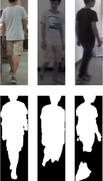
(a) PRCC

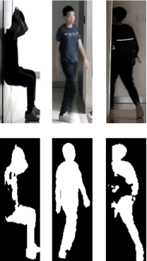
(b) LTCC

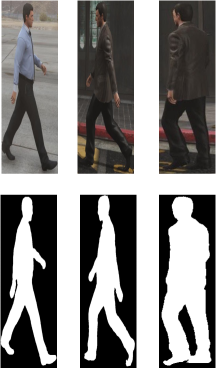
(c) VC-Clothes

Figure 4: Comparison on Image Style and Silhouette Mask Quality on datasets LTCC, PRCC and VC-Clothes.

Performance Evaluation on Deepchange. Deepchange is the latest, largest, and realistic person re-id benchmark with clothes change. We conduct experiments to evaluate the performance of MaskCL and SpCL on this dataset, and report the results in Table 7. Moreover, we also listed the results of supervised training methods using the different backbones provided by Deepchange [48].

Method	Backbone	Deepchange
		mAP	R-1	R-10
Supervised Method
Deepchange [48]	ResNet-50 [14]	9.62	36.6	55.5
Deepchange [48]	ResNet101 [14]	11.0	39.3	57.4
Deepchange [48]	ReIDCaps [24]	13.2	44.2	62.0
Deepchange [48]	ViT B16 [10]	14.9	47.9	67.3
Unsupervised Method
SpCL [12]	ResNet-50[14]	8.90	32.9	47.2
MaskCL	ResNet-50[14]	11.8	39.7	53.7

Table 7: Experimental Results on Deepchange.

Visualization. To gain some intuitive understanding of the performance of our proposed MaskCL, we conduct a set of data visualization experiments on LTCC to visualize selected query samples with the top-10 best matching images in the gallery set, and display the visualization results in Figure 5, where we also show the results of a competitive baseline CACL and more visualisation results are available in the Supplementary Material. Compared to CACL, MaskCL yields more precise matching results. The majority of the incorrect samples matched by CACL are in the same color as the query sample. These findings imply that MaskCL can successfully learn more clothing invariance features and hence identify more precise matches.

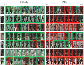
Figure 5: Visualization of the top-10 best matched images on dataset VC-Clothes of CACL and MaskCL. The images with green and red frames are correctly matched and incorrectly matched images, respectively.

Neighbor Searching Selection. To have some intuitive understanding of the model improvement during training process, we visualised the average proportion of correct identity images being sampled by Eq. (10) from semantic neighbor set $\mathcal{A}$, and disaply the curves in Figure 6. As training continue, the proportion also increase. These trends confirm that MaskCL can consequently increasing similarity between different clusters of the same identity hence sampling more correct identiy instance from semantic neighbor sets.

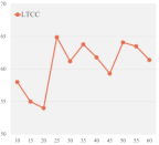
(a) LTCC

(b) Celeb-ReID Series

Figure 6: Visualization of the average proportion of correct identity images being sampled by Eq. (10) from semantic neighbor set $\mathcal{A}$ in training process.

5 Conclusion

We addressed a challenging task: unsupervised long-term person re-id with clothes change. Specifically, we proposed a semantic mask-driven contrastive learning approach, termed MaskCL, which takes the silhouette masks as the semantic prompts in contrastive learning and finds hierarchically semantic neighbor to driven the training. By leveraging the semantic prompt and hierarchically semantic neighbor, MaskCL is able to effectively exploit the invariance within and between RGB images and silhouette masks to learn more effective cross-clothes features. We conducted extensive experiments on five widely-used re-id datasets with clothes change to evaluate the performance. Experimental results demonstrated the superiority of our proposed approach. To the best of our knowledge, this is the first time, unsupervised long-term person re-id problem has been addressed. Our systematic evaluations can serve as a benchmarking ecosystem for the long-term person re-id community.

References

- [1] Slawomir Bak, Peter Carr, and Jean-Francois Lalonde. Domain adaptation through synthesis for unsupervised person re-identification. In ECCV, 2018.
- [2] Xiaobin Chang, Timothy M Hospedales, and Tao Xiang. Multi-level factorisation net for person re-identification. In CVPR, pages 2109–2118, 2018.
- [3] Hao Chen, Benoit Lagadec, and Francois Bremond. Ice: Inter-instance contrastive encoding for unsupervised person re-identification. In ICCV, pages 14960–14969, 2021.
- [4] Hao Chen, Benoit Lagadec, and Francois Bremond. Ice: Inter-instance contrastive encoding for unsupervised person re-identification. In ICCV, pages 14960–14969, 2021.
- [5] Jiaxing Chen, Xinyang Jiang, Fudong Wang, Jun Zhang, Feng Zheng, Xing Sun, and Wei-Shi Zheng. Learning 3d shape feature for texture-insensitive person re-identification. In CVPR, pages 8146–8155, 2021.
- [6] Yoonki Cho, Woo Jae Kim, Seunghoon Hong, and Sung-Eui Yoon. Part-based pseudo label refinement for unsupervised person re-identification. In CVPR, pages 7308–7318, 2022.
- [7] Yoonki Cho, Woo Jae Kim, Seunghoon Hong, and Sung-Eui Yoon. Part-based pseudo label refinement for unsupervised person re-identification. In CVPR, pages 7308–7318, 2022.
- [8] Zuozhuo Dai, Guangyuan Wang, Weihao Yuan, Siyu Zhu, and Ping Tan. Cluster contrast for unsupervised person re-identification. In ACCV, pages 1142–1160, 2022.
- [9] Zuozhuo Dai, Guangyuan Wang, Siyu Zhu, Weihao Yuan, and Ping Tan. Cluster contrast for unsupervised person re-identification. arXiv preprint arXiv:2103.11568, 2021.
- [10] Alexey Dosovitskiy, Lucas Beyer, Alexander Kolesnikov, Dirk Weissenborn, Xiaohua Zhai, Thomas Unterthiner, Mostafa Dehghani, Matthias Minderer, Georg Heigold, Sylvain Gelly, et al. An image is worth 16x16 words: Transformers for image recognition at scale. arXiv preprint arXiv:2010.11929, 2020.
- [11] Yixiao Ge, Zhuowan Li, Haiyu Zhao, Guojun Yin, Shuai Yi, Xiaogang Wang, and Hongsheng Li. Fd-gan: Pose-guided feature distilling gan for robust person re-identification. In NeurIPS, 2018.
- [12] Yixiao Ge, Feng Zhu, Dapeng Chen, Rui Zhao, and Hongsheng Li. Self-paced contrastive learning with hybrid memory for domain adaptive object re-id. In NeurIPS, 2020.
- [13] Xinqian Gu, Hong Chang, Bingpeng Ma, Shutao Bai, Shiguang Shan, and Xilin Chen. Clothes-changing person re-identification with rgb modality only. In CVPR, pages 1060–1069, 2022.
- [14] Kaiming He, Xiangyu Zhang, Shaoqing Ren, and Jian Sun. Deep residual learning for image recognition. In CVPR, 2016.
- [15] Peixian Hong, Tao Wu, Ancong Wu, Xintong Han, and Wei-Shi Zheng. Fine-grained shape-appearance mutual learning for cloth-changing person re-identification. In CVPR, 2021.
- [16] Peixian Hong, Tao Wu, Ancong Wu, Xintong Han, and Wei-Shi Zheng. Fine-grained shape-appearance mutual learning for cloth-changing person re-identification. In CVPR, pages 10513–10522, 2021.
- [17] Ruibing Hou, Bingpeng Ma, Hong Chang, Xinqian Gu, Shiguang Shan, and Xilin Chen. Interaction-and-aggregation network for person re-identification. In CVPR, pages 9317–9326, 2019.
- [18] Yan Huang, Qiang Wu, Jingsong Xu, and Yi Zhong. Celebrities-reid: A benchmark for clothes variation in long-term person re-identification. In IJCNN, 2019.
- [19] Yan Huang, Qiang Wu, Jingsong Xu, and Yi Zhong. Celebrities-reid: A benchmark for clothes variation in long-term person re-identification. In IJCNN, pages 1–8. IEEE, 2019.
- [20] Yan Huang, Qiang Wu, Jingsong Xu, and Yi Zhong. Celebrities-reid: A benchmark for clothes variation in long-term person re-identification. In IJCNN, pages 1–8. IEEE, 2019.
- [21] Yan Huang, Qiang Wu, Jingsong Xu, and Yi Zhong. Celebrities-reid: A benchmark for clothes variation in long-term person re-identification. In IJCNN, pages 1–8. IEEE, 2019.
- [22] Yan Huang, Qiang Wu, JingSong Xu, Yi Zhong, and ZhaoXiang Zhang. Clothing status awareness for long-term person re-identification. In ICCV, pages 11895–11904, 2021.
- [23] Yan Huang, Jingsong Xu, Qiang Wu, Yi Zhong, Peng Zhang, and Zhaoxiang Zhang. Beyond scalar neuron: Adopting vector-neuron capsules for long-term person re-identification. TCSVT, 30(10):3459–3471, 2019.
- [24] Yan Huang, Jingsong Xu, Qiang Wu, Yi Zhong, Peng Zhang, and Zhaoxiang Zhang. Beyond scalar neuron: Adopting vector-neuron capsules for long-term person re-identification. TCSVT, 2019.
- [25] Xin Jin, Tianyu He, Kecheng Zheng, Zhiheng Yin, Xu Shen, Zhen Huang, Ruoyu Feng, Jianqiang Huang, Zhibo Chen, and Xian-Sheng Hua. Cloth-changing person re-identification from a single image with gait prediction and regularization. In CVPR, pages 14278–14287, 2022.
- [26] Diederik P. Kingma and Jimmy Ba. Adam: A method for stochastic optimization. In 3rd International Conference on Learning Representations, 2015.
- [27] Alex Krizhevsky, Ilya Sutskever, and Geoffrey E Hinton. Imagenet classification with deep convolutional neural networks. In NeurIPS, 2012.
- [28] Mingkun L, Li Chun-Guang, and Jun Guo. Cluster-guided asymmetric contrastive learning for unsupervised person re-identification. TIP, 2022.
- [29] Mingkun Li, He Sun, Chaoqun Lin, Chun-Guang Li, and Jun Guo. The devil in the tail: Cluster consolidation plus cluster adaptive balancing loss for unsupervised person re-identification. PR, 129:108763, 2022.
- [30] Minxian Li, Xiatian Zhu, and Shaogang Gong. Unsupervised person re-identification by deep learning tracklet association. In ECCV, 2018.
- [31] Peike Li, Yunqiu Xu, Yunchao Wei, and Yi Yang. Self-correction for human parsing. TPAMI, 2020.
- [32] Wei Li, Xiatian Zhu, and Shaogang Gong. Harmonious attention network for person re-identification. In CVPR, pages 2285–2294, 2018.
- [33] Yu-Jhe Li, Zhengyi Luo, Xinshuo Weng, and Kris M Kitani. Learning shape representations for clothing variations in person re-identification. arXiv preprint arXiv:2003.07340, 2020.
- [34] Jiawei Liu, Zheng-Jun Zha, Di Chen, Richang Hong, and Meng Wang. Adaptive transfer network for cross-domain person re-identification. In CVPR, 2019.
- [35] Peixi Peng, Tao Xiang, Yaowei Wang, Massimiliano Pontil, Shaogang Gong, Tiejun Huang, and Yonghong Tian. Unsupervised cross-dataset transfer learning for person re-identification. In CVPR, 2016.
- [36] Xuelin Qian, Wenxuan Wang, Li Zhang, Fangrui Zhu, Yanwei Fu, Tao Xiang, Yu-Gang Jiang, and Xiangyang Xue. Long-term cloth-changing person re-identification. In ACCV, 2020.
- [37] Xuelin Qian, Wenxuan Wang, Li Zhang, Fangrui Zhu, Yanwei Fu, Tao Xiang, Yu-Gang Jiang, and Xiangyang Xue. Long-term cloth-changing person re-identification. In ACCV, 2020.
- [38] Xuena Ren, Dongming Zhang, and Xiuguo Bao. Person re-identification with a cloth-changing aware transformer. In 2022 International Joint Conference on Neural Networks (IJCNN), pages 1–8. IEEE, 2022.
- [39] Yumin Suh, Jingdong Wang, Siyu Tang, Tao Mei, and Kyoung Mu Lee. Part-aligned bilinear representations for person re-identification. In ECCV, pages 402–419, 2018.
- [40] Yifan Sun, Liang Zheng, Yi Yang, Qi Tian, and Shengjin Wang. Beyond part models: Person retrieval with refined part pooling (and a strong convolutional baseline). In ECCV, pages 480–496, 2018.
- [41] Fangbin Wan, Yang Wu, Xuelin Qian, Yixiong Chen, and Yanwei Fu. When person re-identification meets changing clothes. In CVPRW, 2020.
- [42] Fangbin Wan, Yang Wu, Xuelin Qian, Yixiong Chen, and Yanwei Fu. When person re-identification meets changing clothes. In CVPRW, June 2020.
- [43] Guanshuo Wang, Yufeng Yuan, Xiong Chen, Jiwei Li, and Xi Zhou. Learning discriminative features with multiple granularities for person re-identification. In ACMMM, pages 274–282, 2018.
- [44] Jingya Wang, Xiatian Zhu, Shaogang Gong, and Wei Li. Transferable joint attribute-identity deep learning for unsupervised person re-identification. In CVPR, 2018.
- [45] Kai Wang, Zhi Ma, Shiyan Chen, Jinni Yang, Keke Zhou, and Tao Li. A benchmark for clothes variation in person re-identification. IJIS, 2020.
- [46] Taiqing Wang, Shaogang Gong, Xiatian Zhu, and Shengjin Wang. Person re-identification by video ranking. In ECCV. Springer, 2014.
- [47] Tong Xiao, Hongsheng Li, Wanli Ouyang, and Xiaogang Wang. Learning deep feature representations with domain guided dropout for person re-identification. In CVPR, 2016.
- [48] Peng Xu and Xiatian Zhu. Deepchange: A long-term person re-identification benchmark. arXiv preprint arXiv:2105.14685, 2021.
- [49] Qize Yang, Ancong Wu, and Wei-Shi Zheng. Person re-identification by contour sketch under moderate clothing change. TPAMI, 2019.
- [50] Qize Yang, Ancong Wu, and Wei-Shi Zheng. Person re-identification by contour sketch under moderate clothing change. TPAMI, 2019.
- [51] Mang Ye, Jianbing Shen, Gaojie Lin, Tao Xiang, Ling Shao, and Steven CH Hoi. Deep learning for person re-identification: A survey and outlook. arXiv preprint arXiv:2001.04193, 2020.
- [52] Zhizheng Zhang, Cuiling Lan, Wenjun Zeng, Xin Jin, and Zhibo Chen. Relation-aware global attention for person re-identification. In CVPR, pages 3186–3195, 2020.
- [53] Rui Zhao, Wanli Oyang, and Xiaogang Wang. Person re-identification by saliency learning. TPAMI, 2016.
- [54] Liang Zheng, Yi Yang, and Alexander G Hauptmann. Person re-identification: Past, present and future. arXiv preprint arXiv:1610.02984, 2016.
- [55] Zhedong Zheng, Xiaodong Yang, Zhiding Yu, Liang Zheng, Yi Yang, and Jan Kautz. Joint discriminative and generative learning for person re-identification. In CVPR, pages 2138–2147, 2019.
- [56] Zhedong Zheng, Liang Zheng, and Yi Yang. A discriminatively learned cnn embedding for person reidentification. TOMM, 14(1):1–20, 2017.