On the time scales of spectral evolution of nonlinear waves

Abstract

As presented in Annenkov & Shrira (2009), when a surface gravity wave field is subjected to an abrupt perturbation of external forcing, its spectrum evolves on a “fast” dynamic time scale of $O(\varepsilon^{-2})$, with $\varepsilon$ a measure of wave steepness. This observation poses a challenge to wave turbulence theory that predicts an evolution with a kinetic time scale of $O(\varepsilon^{-4})$. We revisit this unresolved problem by studying the same situation in the context of a one-dimensional Majda-McLaughlin-Tabak (MMT) equation with gravity wave dispersion relation. Our results show that the kinetic and dynamic time scales can both be realised, with the former and latter occurring for weaker and stronger forcing perturbations, respectively. The transition between the two regimes corresponds to a critical forcing perturbation, with which the spectral evolution time scale drops to the same order as the linear wave period (of some representative mode). Such fast spectral evolution is mainly induced by a far-from-stationary state after a sufficiently strong forcing perturbation is applied. We further develop a set-based interaction analysis to show that the inertial-range modal evolution in the studied cases is dominated by their (mostly non-local) interactions with the low-wavenumber “condensate” induced by the forcing perturbation. The results obtained in this work should be considered to provide significant insight into the original gravity wave problem.

1 Introduction

Wave turbulence theory (WTT) describes the statistical properties of ensembles of weakly nonlinear interacting waves, with rich applications in many physical contexts, e.g., ocean waves (Zakharov & Filonenko, 1967; Nazarenko & Lukaschuk, 2016), acoustics (L’vov et al., 1997), magnetohydrodynamics (Galtier et al., 2000), quantum turbulence (Nazarenko & Onorato, 2006), and others. The centrepiece of WTT is a wave kinetic equation (WKE), which describes the time evolution of the wave action spectrum as an integral over wave-wave interactions. The WKE yields a stationary Kolmogorov-Zakharov (KZ) power-law solution associated with a constant flux, which has been observed in many wave systems.

Quantitative validations of the WKE and its predictions in different physical contexts have been a prominent topic in the wave turbulence community for decades. These studies include extensive numerical and experimental validations of the spectral slope and energy flux (or Kolmogorov constant) of the KZ solutions (e.g. Pan & Yue, 2014; Hrabski & Pan, 2022; Zhang & Pan, 2022a; Falcon & Mordant, 2022; Zhu et al., 2023), numerical validation of the initial spectral evolution predicted by the WKE (e.g. Zhu et al., 2022; Banks et al., 2022), and rigorous mathematical justification of the WKE (e.g. Deng & Hani, 2021, 2023; Buckmaster et al., 2021). Although successes in verifying the WKE have been reported in many cases, situations where WKE predictions fail have also been identified, such as circumstances associated with finite-size effects (e.g. L’vov & Nazarenko, 2010; Hrabski & Pan, 2020; Zhang & Pan, 2022b), coherent structures in the field (e.g. Rumpf, Newell & Zakharov, 2009), and the strong turbulence regime (e.g. Chibbaro, De Lillo & Onorato, 2017).
In spite of the significant advancement in understanding the WKE, there exist a series of relevant studies on surface gravity waves that remain largely unexplained. A representative work of this series is the paper by Annenkov & Shrira (2009), which considers the spectral evolution when a stationary gravity wave field is subjected to an abrupt perturbation of external wind forcing. According to the WKE of gravity waves, in the form of $\partial n/\partial t\sim n^{3}$ with $n\sim\varepsilon^{2}$ the wave action spectrum, one would expect an evolution with the kinetic time scale $O(\varepsilon^{-4})$. However, simulations of the dynamic equation, specifically the Zakharov equation (Zakharov, 1968), show a faster evolution with a dynamic time scale of $O(\varepsilon^{-2})$. This “fast” spectral evolution is also observed in wave-tank experiments (e.g. Autard, 1995; Waseda, Toba & Tulin, 2001) and field studies (van Vledder & Holthuijsen, 1993) when the wind exhibits a sudden change in speed or direction, as well as numerical simulations for the initial evolution of some wave spectra (Dysthe et al., 2003). In a study by Annenkov & Shrira (2018), an attempt is made in explaining the fast spectral evolution using the so-called generalised WKE, but only limited success is achieved. This unexplained issue is concerning since the WKE of surface gravity waves (also known as Hasselmann’s kinetic equation (Hasselmann, 1962)) is currently used in modern wave modelling codes whose reliability is pertinent to weather forecasting, climate modelling, and navigation (Janssen, 2004).
In this paper, we revisit the spectral evolution problem in the context of the one-dimensional (1D) Majda–McLaughlin–Tabak (MMT) equation with gravity wave dispersion relation. The MMT model is favourable in the sense that it captures the essential dynamics of wave turbulence while being exempt from the complexities associated with surface gravity waves (such as the need to remove quadratic nonlinearity terms in deriving the WKE). In addition, with a 1D model, we are able to perform large numbers of ensemble simulations, with which the statistical properties can be reliably computed through ensemble averages. We will conduct the study and analysis closely following Annenkov & Shrira (2009), i.e., with numerical setups and evaluation of properties as consistent as possible, except using the 1D MMT model.
For a given stationary wave field, we show that evolution with kinetic and dynamic time scales can be observed for weaker and stronger forcing perturbations, respectively. The transition from the former to the latter regime corresponds to a forcing perturbation that triggers a spectral evolution time scale comparable to the linear time scale, i.e., the wave period of some representative mode, violating the basis of the WKE. We further show, through a study varying the energy of the base stationary wave field, that this violation of time scale separation is primarily a result of the spectrum far from the stationary state after a sufficiently strong forcing perturbation is applied, rather than the increase of overall nonlinearity level of the wave field. We finally develop a set-based interaction analysis, which allows us to understand that the spectral evolution for modes in the inertial range is predominantly governed by their (mostly non-local) interactions with the low-wavenumber condensate (or regions sufficiently filled with energy) induced by the forcing perturbation.

2 Methodology

2.1 The MMT model

We study the evolution of random wave fields through the one-dimensional MMT equation (Majda et al., 1997), which is a family of nonlinear dispersive wave equations widely used to study wave turbulence problems (e.g. Cai et al., 1999; Zakharov, Pushkarev & Dias, 2004; Chibbaro, De Lillo & Onorato, 2017; Hrabski & Pan, 2022),

$$\textnormal{i}\frac{\partial\psi}{\partial t}={\lvert{\partial_{x}}\rvert}^{\alpha}\psi+\lambda{\lvert{\partial_{x}}\rvert}^{\beta/4}({\big{\lvert}{\lvert{\partial_{x}}\rvert}^{\beta/4}\psi\big{\rvert}}^{2}{\lvert{\partial_{x}}\rvert}^{\beta/4}\psi),$$ (1)

where $\psi(x,t)$ is a field taking complex values. The parameter $\beta$ controls the nonlinearity formulation and $\alpha$ controls the dispersion relation $\omega(k)=|k|^{\alpha}$ with $\omega$ the frequency and $k$ the wavenumber. $\lambda=-1$ and $1$ represent the focusing (defocusing) nonlinearity, respectively (Cai et al., 2001). The MMT equation (1) conserves both the total Hamiltonian and wave action. In our study, we use $\alpha=1/2$ to mimic the dispersion of surface gravity waves, and use $\beta=0$ for convenience which is consistent with a portion of the original study of the MMT equation (Majda et al., 1997) and is widely used in other studies (e.g. Cai et al., 1999; Rumpf & Newell, 2013; Rumpf & Sheffield, 2015). We note that although $\beta=0$ is not entirely representative of surface gravity waves, the primary conclusion of the paper does not depend on a specific choice of $\beta$. We will present the results for the defocusing case ($\lambda=1$) in the main paper, and those for the focusing case in the Appendix B, with both cases exhibiting similar physics regarding the spectral evolution time scales.

From a standard wave turbulence consideration, a statistical description of the wave field can be obtained by defining the wave action spectrum $n_{k}=\langle{\lvert{\hat{\psi}_{k}}\rvert}^{2}\rangle$, with $\hat{\psi}_{k}$ the Fourier transform of $\psi$ and the angle brackets denoting an ensemble average. Under conditions of weak nonlinearity, random phases, and infinite domain, the time evolution of $n_{k}$ is governed by the wave kinetic equation (WKE) (for $\beta=0$),

$$\begin{split}\frac{\partial n_{k}}{\partial t}=4\pi\int(n_{1}n_{2}n_{3}+n_{1}n_{2}n_{k}-n_{1}n_{3}n_{k}-n_{2}n_{3}n_{k})\\ \times\delta(\omega_{1}+\omega_{2}-\omega_{3}-\omega)\delta(k_{1}+k_{2}-k_{3}-k)\textnormal{d}k_{1}\textnormal{d}k_{2}\textnormal{d}k_{3}\end{split}$$ (2)

where $\delta$ is the Dirac delta function. According to (2), the spectrum evolves with a kinetic time scale, i.e., $n_{k}$ experiences significant change with a time scale $O(\varepsilon^{-4})$, and $\partial n_{k}/\partial t\sim O(\varepsilon^{6})$ over the evolution, with $\varepsilon\sim\sqrt{n_{k}}$ a measure of wave steepness. Hereafter, we will refer to these relations as kinetic scaling in this paper, which is in contrast to the dynamic scaling of a time scale $O(\varepsilon^{-2})$ and $\partial n_{k}/\partial t\sim O(\varepsilon^{4})$ that one can directly obtain from (1).

2.2 Numerical procedure

We simulate (1) with 4096 modes (before de-aliasing) on a periodic domain of size $L=2\pi$, with the addition of forcing and dissipation terms. The forcing is in white-noise form, given by

$$F=\begin{cases}F_{r}+\textnormal{i}F_{i},&4\leq k\leq 13,\\ 0,&\text{otherwise},\end{cases}$$ (3)

with $F_{r}$ and $F_{i}$ independently drawn from a Gaussian distribution $\mathcal{N}(0,\sigma^{2})$. The dissipation is introduced with the addition of two hyperviscosity terms

$$\left.\begin{aligned} D_{1}=\begin{cases}-\textnormal{i}\nu_{1}\hat{\psi}_{k},&k\geq 900,\\ 0,&\text{otherwise},\end{cases}\\ D_{2}=\begin{cases}-\textnormal{i}\nu_{2}\hat{\psi}_{k},&k\leq 4,\\ 0,&\text{otherwise},\end{cases}\end{aligned}\right\}$$ (4)

at small and large scales, respectively. Since the MMT model supports the inverse cascade, it is necessary to use large-scale dissipation to avoid energy accumulation at large scales. The dissipation coefficients are fixed to be $\nu_{1}=1\times 10^{-14}(k-900)^{8}$ and $\nu_{2}=3k^{-4}$ for all numerical experiments. The numerical schemes used for the simulation are discussed in detail in previous papers (Hrabski & Pan, 2020, 2022).

In order to reproduce the physical scenario as in Annenkov & Shrira (2009), we perform the simulation with two stages. In stage 1, we simulate (1) with (3) and (4) using $\sigma=\sigma_{0}$ for sufficient time to reach a stationary wave field (and spectrum), starting from an initial spectrum that exponentially decays in $|k|$. In stage 2, we add a perturbation $\Delta\sigma$ to the forcing magnitude (leading to $\sigma=\sigma_{0}+\Delta\sigma$) and study how the spectrum evolves subject to the perturbation. In both stages, we use a time step $\Delta t=0.012$. For the main cases studied in this paper, we consider the stationary state obtained with forcing $\sigma_{0}=0.004$ in stage 1, and consider forcing perturbations $\Delta\sigma\in[0.033,1.461]$ in stage 2 that is sufficient to cover the physical regimes of our interest. The process is simulated with an ensemble of 65000 simulations with different random seeds in the forcing, and all statistical results related to $n_{k}$ presented below are obtained directly from the average over the whole or part of the ensemble that is statistically convergent.

3 Results

Figure 1 shows the evolution of a spectrum in a typical case with $\sigma_{0}=0.004$ and $\Delta\sigma=0.033$. We see that a stationary power-law spectrum forms at the end of stage 1, which serves as the base state of the problem. As a forcing perturbation is excited in stage 2, the forcing scales (as well as scales slightly larger than that) first experience an abrupt growth, forming a condensate at large scales. The growth is then propagated to smaller scales, which eventually fill in the full spectral range and form the final stationary power-law spectrum. We note that such behaviour regarding the propagation of growth is closely related to the fact that (1) under selected values of $\alpha$ and $\beta$ is an infinite capacity system (Nazarenko, 2011; Newell & Rumpf, 2011). Hereafter, for simplicity, we assign time $t=0$ to the stationary state before a forcing perturbation is applied, and $t=t_{f}$ to the time when the final stationary state is formed. We measure the wave steepness of each state as $\varepsilon=\sqrt{E_{L}}$ with $E_{L}$ the linear energy (or Hamiltonian) of the system. Accordingly, we use $\varepsilon_{0}$ and $\varepsilon_{f}$ as the wave steepness at $t=0$ and $t=t_{f}$. We note that this definition of $\varepsilon$ is consistent with that in Annenkov & Shrira (2009) with the additional factor of constant peak wavenumber $k_{p}$ omitted in our definition.

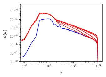
Figure 1: A typical case of the evolution of wave action spectrum, where $n(k,0)$ (—) and $n(k,t_{f})$ (—) represent the stationary spectra before the forcing perturbation (stage 1) and after sufficient evolution with forcing perturbation applied (stage 2). The intermediate spectra in the evolution between $n(k,0)$ and $n(k,t_{f})$ are plotted ($---$).

We are interested in the growth rate in the transient period in stage 2, based on which we can evaluate $\partial n_{k}/\partial t$ and the associated scaling with wave steepness. For this purpose, we follow Annenkov & Shrira (2009) to measure $\partial n_{k}/\partial t$ for a given mode $k$ using data over the interval of 5-40% of the total modal growth. More specifically, if we define a normalised wave action spectrum $\tilde{n}(k,t)=(n(k,t)-n(k,0))/(n(k,t_{f})-n(k,0))$, we can then measure $\partial\tilde{n}_{k}/\partial t$ over the range of $\tilde{n}_{k}\in[5\%,40\%]$ via a least-square fit, and then scale back to compute $\partial n_{k}/\partial t$. Figure 2 shows the evolution of $\tilde{n}(k,t)$ for three selected modes in the inertial range, as well as the growth rate evaluated using the $[5\%,40\%]$ interval. It is clear that the evaluated growth rate over the chosen interval is sufficient to capture the instantaneous spectral growth after the forcing perturbation is imposed.

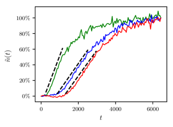
Figure 2: A typical case of the evolution of modal wave action at three wavenumbers $k=150$ (—), $k=500$ (—), $k=800$ (—) in the inertial-range. The growth rates $\partial\tilde{n}_{k}/\partial t$ measured over the range of $\tilde{n}_{k}\in[5\%,40\%]$ are indicated ($---$).

3.1 Scaling of spectral growth rate with $\varepsilon$

To evaluate the scaling of $\partial n_{k}/\partial t$ with the wave steepness $\varepsilon$, we use the final-state $\varepsilon=\varepsilon_{f}$ as a representative value of the wave steepness for the case (cf. Annenkov & Shrira, 2009). Figure 3 shows $\partial n_{k}/\partial t$ of three modes in the inertial range for a broad range of $\varepsilon\in[0.022,0.124]$, obtained from 22 cases with $\Delta\sigma\in[0.033,1.461]$ starting from a base state with $\varepsilon_{0}=0.010$ resulting from $\sigma_{0}=0.004$. As we see in figure 3, the kinetic scaling $\partial n_{k}/\partial t\sim O(\varepsilon^{6})$ is realised in the range of $\varepsilon\lesssim 0.05$, corresponding to small $\Delta\sigma$ with $\Delta\sigma\lesssim 0.36$. For larger forcing perturbations, we find dynamic scaling in the range of $\varepsilon\gtrsim 0.05$. We remark that in the previous work for gravity waves (Annenkov & Shrira 2009), only dynamic scaling is observed. This is possibly due to their studies only being conducted for strong forcing perturbations, or other reasons that we will leave for future study.

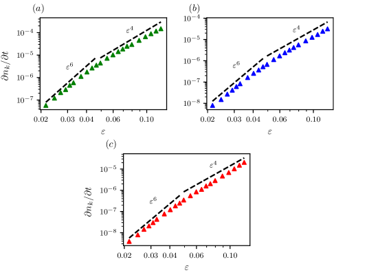
Figure 3: Rate of spectral evolution $\partial n_{k}/\partial t$ as a function of nonlinearity $\varepsilon$ for (a) $k=150$ ($\blacktriangle$), (b) $k=500$ ($\blacktriangle$), and (c) $k=800$ ($\blacktriangle$), with the kinetic $\varepsilon^{6}$ and dynamic $\varepsilon^{4}$ scalings indicated by the dashed lines.

We next investigate why the “fast” dynamic scaling becomes relevant for the spectral evolution, a critical question that is not answered in previous works (e.g. Annenkov & Shrira, 2006, 2009, 2018). The realisation of dynamic scaling indicates that the WKE (2) (or more generally, wave turbulence theory) must break down. One situation in which this could happen is a violation of time scale separation, i.e., when the nonlinear modal time scale becomes comparable to the linear modal time scale. In particular, the linear time scale of a mode is given by the modal wave period

$$\tau_{L}=\frac{2\pi}{\omega}.$$ (5)

The nonlinear time scale can be computed in our case as the spectral evolution time scale

$$\tau_{NL}=\frac{n_{k}}{\frac{\partial n_{k}}{\partial t}},$$ (6)

with $\partial n_{k}/\partial t$ evaluated from our numerical data. Hereafter, we will also use the terminology “spectral evolution time scale” which is somewhat more illuminating than “nonlinear time scale”. In addition, we note that in many cases (e.g. Newell, Nazarenko & Biven, 2001; Newell & Rumpf, 2011) the nonlinear time scale is taken as the kinetic time scale, which is not appropriate here since $\partial n_{k}/\partial t$ in (6) is evaluated by the dynamic equation instead of the WKE. The ratio of the spectral evolution and linear time scales is given by

$$\rho=\frac{\tau_{NL}}{\tau_{L}}.$$ (7)

The WKE is expected to be valid only when the time scales are well separated with $\rho\gg O(1)$.

To study the time scale separation in our cases, we first mention that $\rho$ is, in general, a function of $k$, as shown in two typical cases in figure 4 for $\Delta\sigma=0.033$ and $1.461$. We see that $\rho$ generally increases with $k$ in a power-law form, which is related to our choice $\beta=0$ in (1) (which makes the nonlinear strength weaker for high $k$ than that from a positive $\beta$). Additionally, we see that as $\Delta\sigma$ increases from the former values to the latter, $\rho$ generally drops below $O(1)$, indicating the breakdown of the WKE in the latter case. We next seek to understand the relationship between the time scale separation and the transition to the dynamic scaling of spectral evolution. To this end, we first note that the transition to dynamic scaling at all inertial-range wavenumbers (see figure 3) occurs at a similar forcing perturbation, indicating that the WKE breaks down for the overall spectral range instead of a particular wavenumber. Therefore, we evaluate $\rho$ at a representative wavenumber $k=100$, which leads to a relatively low value of $\rho$ in the inertial range as an assessment of the overall validity of WTT. We plot in figure 5 $\rho(k=100)$ as a function of $\varepsilon$, overlaid with the previous plot of $\partial n_{k}/\partial t$ for $k=500$ (as an example). We see that the transition to dynamic scaling occurs at $\rho\approx 4\sim O(1)$, which indicates that the dynamic scaling range is consistent with the failure of the WKE due to the violation of time scale separation. We also remark that if a different value of $k$ is chosen for the evaluation of $\rho$, we will end up with a slightly different transition value of $\rho$ which is at most approximately 10 as one can estimate from figure 4.

Figure 4: Ratio of time scales $\rho$ as a function of $k$ for cases with $\Delta\sigma=0.033$, $\varepsilon=0.022$ ($\bullet$) and $\Delta\sigma=1.461$, $\varepsilon=0.124$ ($\bullet$).

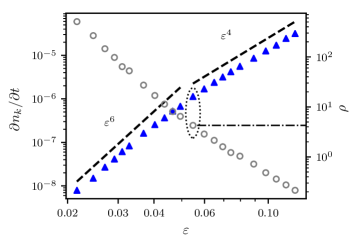
Figure 5: Ratio of the time scales $\partial n_{k}/\partial t(k=500)$ (left axis, $\blacktriangle$) and $\rho(k=100)$ (right axis, $\circ$) as functions of $\varepsilon$. The region of transition from kinetic to dynamic scaling is circled, with the corresponding value of $\rho$ indicated ($-\cdot-$).

While the above analysis reveals the reduction of $\tau_{NL}$ as the underlying reason for the transition to dynamic scaling, the cause of this reduction remains unclear. In many previous studies, the reduction of $\tau_{NL}$ is attributed to the increase of nonlinearity level, which transits the dynamics into a strong turbulence regime (often associated with intermittency) where the WKE becomes irrelevant. However, we argue that this is not the major reason for the transition to dynamic scaling observed in our study, which is instead mainly triggered by the spectrum being too far from the stationary spectrum after a strong forcing perturbation is applied. To provide evidence for this argument, we repeat our analysis for three additional situations with higher values of $\varepsilon_{0}$. Figure 6 shows that the transition value of $\varepsilon$ increases with $\varepsilon_{0}$ following an approximately linear form of $\varepsilon\sim\varepsilon_{0}$, and that these transitions all correspond to $\rho(k=100)\sim O(1-10)$, which is in agreement with the above analysis. This is consistent with the argument about the transition caused by a far-from-stationary spectrum induced by a strong forcing perturbation, since the deviation of the spectrum from the stationary state is approximately measured by the difference between $\varepsilon$ and $\varepsilon_{0}$, which does not change significantly in all cases. Moreover, figure 6 is in clear contradiction with a transition induced by a high nonlinearity level (or strong turbulence), in which case one would otherwise expect that the transition occurs at approximately the same $\varepsilon$ for different $\varepsilon_{0}$.

The failure of the WKE due to the spectrum far from the stationary state can also be reasoned from a thought experiment: given a spectrum, one can assume a priori that the WKE is valid, based on which $\partial n_{k}/\partial t$ can be computed. Such computed $\partial n_{k}/\partial t$ may a posteriori be found to violate the condition of $\rho\gg O(1)$ that invalidates the assumed WKE (see examples for internal gravity waves in Lvov, Polzin & Yokoyama (2012) and Eden, Pollmann & Olbers (2019)). In this view, as the spectrum deviates from the stationary state, there exists a critical spectral form (even if the nonlinearity level is relatively low) that drives fast evolution beyond which the WKE fails.

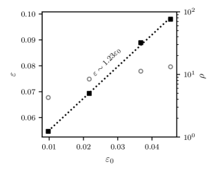
Figure 6: Values of $\varepsilon$ (left axis, $\blacksquare$) and $\rho(k=100)$ (right axis, $\circ$) corresponding to transition to dynamic scaling for each base nonlinearity level $\varepsilon_{0}$, with a linear fitting ($\cdots$) and relation indicated.

3.2 Dominant interactions in modal growth

From section § 3.1 we understand that the forcing perturbation (and the associated condensate) creates a deviation of the spectrum from the stationary state, which drives the subsequent spectral evolution. It is therefore reasonable to further argue that the inertial-range modal growth is dominated by direct interaction with the condensate peak, or at least non-local interactions with large-scale features. In this section, we verify this hypothesis using a new set-based interaction analysis. We remark that this is not a trivial task in the sense that these interactions cannot be analysed on the basis of the WKE, but rather must be analysed based on the dynamic equation (1) which is valid for all cases.

To start, we first define a set-based modal growth rate $\partial n_{k}/\partial t\rvert_{A}$ to be the evolution rate of $n_{k}$ due to the interaction of mode $k$ with $k_{i}\in A$ for $i=1,2,3$. By definition, if $A=\Lambda\equiv[-k_{max},k_{max}]$ (i.e., the full spectral range with $k_{max}=1024$ after de-aliasing), then $\partial n(k)/\partial t\rvert_{A}=\partial n(k)/\partial t$. For $A\in\Lambda$, we can compute $\partial n(k)/\partial t\rvert_{A}$ by invoking (1) as

$$\frac{\partial n(k)}{\partial t}\biggr{\rvert}_{A}=\sum_{k_{1}\in A,k_{2}\in A,k_{3}\in A}2\textnormal{Im}\langle\hat{\psi}_{1}\hat{\psi}_{2}\hat{\psi}^{\ast}_{3}\hat{\psi}^{\ast}_{k}\rangle\delta^{12}_{3k},$$ (8)

where $\delta^{12}_{3k}\equiv\delta(k_{1}+k_{2}-k-k_{3})$ and the ${\hat{\psi}}_{k}^{*}$ denotes the complex conjugate of $\psi_{k}$. The direct computation of (8) in spectral space is very expensive, with a computational complexity of $O(k_{max}^{3})$ for each ensemble member of the group at each time instant (the ensemble and the time average are then used to compute the operator $\langle\,\rangle$). The computational cost can be significantly reduced if the evaluation of (8) can be performed in physical space, which turns out to be possible as we detail in Appendix A, with the result

$$\frac{\partial n(k)}{\partial t}\biggr{\rvert}_{A}\equiv 2\textnormal{Im}\langle\hat{\psi}^{*}_{k}\mathcal{F}[B_{A}(\psi(x))B_{A}(\psi(x))B_{A}(\psi^{*}(x))]\rangle,$$ (9)

where $\mathcal{F}[\,]$ represents the Fourier transform, and $B_{A}$ represents a Fourier-domain filter to select modes in $A$ for a quantity in physical domain. The computation of (9) only requires a number of fast Fourier transforms which is much less expensive than that for (8).

In order to sort out the dominant interactions that lead to the growth of a mode $k_{0}$, we evaluate $\partial n(k_{0})/\partial t\rvert_{A}$ by setting $A=[-k_{max},-k_{A}]\cup[k_{A},k_{max}]$ with $k_{A}$ varying in $[1,k_{0}]$. Therefore, for fixed $k_{0}$, $\partial n(k_{0})/\partial t\rvert_{A}$ can be considered as a function of $k_{A}$. As $k_{A}$ decreases from $k_{0}$ to 1, $\partial n(k_{0})/\partial t\rvert_{A}$ accounts for more non-local interactions with large scales (which is more important than interactions with small scales that are not particularly studied in current setting). Figure 7 plots $\partial n(k_{0})/\partial t\rvert_{A}$ (normalised by $\partial n(k_{0})/\partial t$) as a function of $k_{A}$ for three selected values of $k_{0}$ in the inertial range, and for two cases of $\varepsilon=0.022$ and $0.124$ corresponding to regimes of kinetic and dynamic scaling, respectively. We first see that, for each case, the leftmost point (i.e., when $k_{A}=1$) recovers the total $\partial n(k_{0})/\partial t$, which can be considered as a validation of our computation. For $k_{A}$ relatively close to $k_{0}$, local interactions are represented, with those for higher nonlinearity levels showing stronger fluctuations, i.e., stronger local interactions. Nevertheless, for all cases, there exists a wavenumber $k_{c}$ (marked in each figure) at which the normalised $\partial n(k_{0})/\partial t\rvert_{A}$ becomes close to zero or negative. This means that the overall local interactions in the range $[k_{c},k_{0}]$ do not contribute much (or even contribute negatively) to the total $\partial n(k_{0})/\partial t$. The major contribution to recover $\partial n(k_{0})/\partial t$ occurs for a range immediately left of $k_{c}$, where the normalised $\partial n(k_{0})/\partial t\rvert_{A}$ grows quickly from the minimum value to 1. This range features non-local interactions with scale separation of $k_{c}/k_{0}\sim O(0.1)$ (see table 1 for exact numbers) for all cases shown in the figure. The fact that $k_{c}$ increases with $k_{0}$ indicates that the large scales participating in the dominant interactions propagate to higher wavenumbers. For $k_{0}=150$, the non-local interactions mainly involve the forced condensate range up to about $k_{c}\sim O(10)$. For $k_{0}=500$ and $k_{0}=800$, the small-wavenumber range sufficiently filled with energy during the propagation of the perturbation becomes the dominant interacting modes.

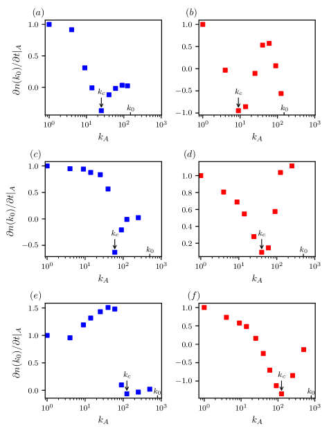
Figure 7: Rate of spectral evolution $\partial n(k_{0})/\partial t\rvert_{A}$, normalized by $\partial n(k_{0})/\partial t$, as a function of $k_{A}$, for three wavenumbers (a, b) $k_{0}=150$, (c, d) $k_{0}=500$ and (e, f) $k_{0}=800$. The columns on the left (a, c, e) and on the right (b, d, f) are for cases with $\Delta\sigma=0.033$ and $1.461$ in the kinetic and dynamic scaling regimes, respectively. The positions of $k_{c}$ (where minimum value $\partial n(k_{0})/\partial t\rvert_{A}$ is achieved) and $k_{0}$ are indicated in each sub-figure.

Nonlinearity $\varepsilon$	Wavenumber of interest $k_{0}$	Wavenumber at minimum $k_{c}$	$k_{c}/k_{0}$
0.022	150	25	0.167
	500	60	0.120
	800	125	0.156
0.124	150	9	0.060
	500	40	0.080
	800	125	0.156

Table 1: Values of $k_{c}$ and $k_{c}/k_{0}$ for all test cases.

In summary, the analysis here implies that, for all forcing perturbations considered, the inertial-range modal growth is mainly driven by the non-local interactions of the modes with large scales. The local interactions introduce some fluctuations that are stronger for higher-nonlinearity cases, but are sufficiently decayed when enlarging the spectral range around $k_{0}$ and before the dominant non-local interactions take place. We also mention that in the low-nonlinearity cases, the non-local interactions (especially those with the condensate) can be approximated by a diffusion equation recently derived in Korotkevich et al. (2023) for four-wave systems.

4 Conclusion and discussions

In this paper, we numerically study the time scales of spectral evolution of nonlinear waves under perturbed forcing, in order to understand the previously identified “fast” spectral evolution with the dynamic time scale contradicting the prediction from the WKE. Our study is conducted in the context of 1D MMT equation, that mimics the wave turbulence of surface gravity waves free of other associated complexities. We show that both kinetic and dynamic time scales can become relevant for spectral evolution depending on the magnitude of the perturbed forcing applied to the stationary spectrum. The kinetic scaling occurs at weaker forcing perturbations, which transits to dynamic scaling as the forcing perturbation becomes strong enough, with the transition corresponding to the situation of the spectral evolution (or nonlinear) time scale dropping to the same level as the linear time scale. Such decrease in nonlinear time scale is mainly induced by the spectrum being far from the stationary state after the forcing perturbation is applied, instead of solely due to the usually-considered cause of increasing nonlinearity level. Finally, through a new set-based interaction analysis, we find that the inertial-range spectral growth is dominated by its nonlocal interactions with the forced condensate or large scales sufficiently filled with energy throughout all nonlinearity levels.

Our study suggests that in assessing the validity of the WKE for transient spectra, the specific spectral forms need to be considered, in conjunction with the traditionally considered factors such as weak/strong turbulence and intermittency. Although we will consider another study directly regarding surface gravity waves as our future work, the study here itself provides significant insight into the observed dynamic time scale in the spectral evolution of surface gravity waves under perturbed forcing (Annenkov & Shrira, 2009). The established interpretation may also apply to the initial evolution of the wave spectrum, which is sometimes reported to be on the dynamic scale (Dysthe et al., 2003) and sometimes precisely matches the prediction by the WKE (Zhu et al., 2022).

5 Citations and references

Acknowledgements. The authors acknowledge the Simons Foundation for funding support for this work, and thank Prof. Miguel Onorato for helpful discussions on this work during the Simons Collaboration on Wave Turbulence Annual Meeting in 2022.

Declaration of interests. The authors report no conflict of interest.

Appendix A Fast computation for set-based interaction analysis

We start by re-ordering (8) (by interchanging allowed operations) as

$$\frac{\partial n(k)}{\partial t}\biggr{\rvert}_{A}=2\textnormal{Im}\langle\hat{\psi}^{*}_{k}\sum_{k_{1}\in A,k_{2}\in A,k_{3}\in A}\hat{\psi}_{1}\hat{\psi}_{2}\hat{\psi}^{*}_{3}\delta^{12}_{3k}\rangle.$$ (10)

The significant computational cost comes from the summation term on the right-hand side of (10). To reduce the computational cost, we can consider the summation term as the Fourier transform of a physical-space quantity:

$$\sum_{k_{1}\in A,k_{2}\in A,k_{3}\in A}\hat{\psi}_{1}\hat{\psi}_{2}\hat{\psi}^{*}_{3}\delta^{12}_{3k}=\mathcal{F}[B_{A}(\psi(x))B_{A}(\psi(x))B_{A}(\psi^{*}(x))],$$ (11)

where $\mathcal{F}[\,]$ represents the Fourier transform, and $B_{A}$ represents a Fourier-domain filter to select modes in $A$ for a physical domain function $\psi(x)$. Equation (11) can be understood from the convolution theorem for three functions, i.e., spectral domain convolution is equal to the physical domain multiplication. One can also directly confirm that this is true by starting from the right-hand side and expressing each $B_{A}(\psi(x))$ as the summation of Fourier modes:

$$\frac{1}{2\pi}\int e^{-ikx}\sum_{k_{1}\in A}\hat{\psi}(k_{1})e^{ik_{1}x}\sum_{k_{2}\in A}\hat{\psi}(k_{2})e^{ik_{2}x}\sum_{k_{3}\in A}\hat{\psi}^{*}(k_{3})e^{-ik_{3}x}dx$$ (12)

which can be re-organized as

$$\frac{1}{2\pi}\int\sum_{k_{1}\in A,k_{2}\in A,k_{3}\in A}\hat{\psi}(k_{1})\hat{\psi}(k_{2})\hat{\psi}^{*}(k_{3})e^{i(k_{1}+k_{2}-k-k_{3})x}dx.$$ (13)

We see that (13) is the same as the left hand side of (10) after considering $\frac{1}{2\pi}\int e^{i(k_{1}+k_{2}-k-k_{3})x}=\delta(k_{1}+k_{2}-k-k_{3})$.

Appendix B Results from cases with focusing nonlinearity

In this appendix, we summarize results from cases with focusing nonlinearity, i.e., $\lambda=-1$ in (1). All other parameters in the study are kept consistent with those in the defocusing cases reported in the main paper. Figures 8 and 9 show respectively the scaling of $\partial n_{k}/\partial t$ with $\varepsilon$ and the study regarding $\rho$, as counterparts of figure 3 and 4 in the main paper. It is clear from these figures that the main conclusion made for the defocusing case also applies to the focusing case.

Figure 8: See caption for figure 3, but for the focusing case.

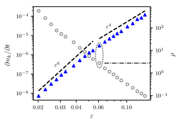
Figure 9: See caption for figure 4, but for the focusing case.

References

- (1)
- Annenkov & Shrira (2001) Annenkov, S.Y. & Shrira, V.I. 2001 Numerical modelling of water-wave evolution based on the Zakharov equation. J. Fluid Mech. 449, 341-371.
- Annenkov & Shrira (2006) Annenkov, S.Y. & Shrira, V.I. 2006 Role of non-resonant interactions in the evolution of nonlinear random water wave fields. J. Fluid Mech. 561, 181-207.
- Annenkov & Shrira (2009) Annenkov, S.Y. & Shrira, V.I. 2009 ”Fast” Nonlinear Evolution in Wave Turbulence. Phys. Rev. Lett. 102 (2), 024502.
- Annenkov & Shrira (2018) Annenkov, S.Y. & Shrira, V.I. 2018 Spectral evolution of weakly nonlinear random waves: kinetic description versus direct numerical simulation. J. Fluid Mech. 844, 766-795.
- Autard (1995) Autard, L. 1995 Ph.D. Thesis. Université Aix-Marseille I and II.
- Banks et al. (2022) Banks, J. W., Buckmaster, T., Korotkevich, A. O., Kovačič, G. & Shatah, J. 2022 Direct Verification of the Kinetic Description of Wave Turbulence for Finite-Size Systems Dominated by Interactions among Groups of Six Waves. Phys. Rev. Lett. 129 (3), 034101.
- Buckmaster et al. (2021) Buckmaster, T., Germain, P., Hani, Z. & Shatah, J. 2021 Onset of the wave turbulence description of the longtime behavior of the nonlinear Schrödinger equation. Invent. Math. 225 (3), 787-855.
- Cai et al. (1999) Cai, D., Majda, A.J., McLaughlin, D.W., Tabak, E.G. 1999 Spectral Bifurcations in Dispersive Wave Turbulence. Proc. Natl Acad. Sci. 96 (25), 14216-14221.
- Cai et al. (2001) Cai, D., Majda, A.J., McLaughlin, D.W., Tabak, E.G. 2001 Dispersive wave turbulence in one dimension. Physica D 152, 551-572.
- Chibbaro, De Lillo & Onorato (2017) Chibbaro, S., De Lillo, F., Onorato, M. 2017 Weak versus strong wave turbulence in the Majda-McLaughlin-Tabak model. Phys. Rev. Fluids 2 (5), 052607.
- Deng & Hani (2021) Deng, Y. & Hani, Z. 2021 On the derivation of the wave kinetic equation for NLS. Forum Maths Pi 9 (e6).
- Deng & Hani (2023) Deng, Y. & Hani, Z. 2023 Full derivation of the wave kinetic equation. Invent. math. arXiv:2104.11204v4.
- Dysthe et al. (2003) Dyachenko, K.B., Trulsen, K., Krogstad, H.E. & Socquet-Juglard V. E 2003 Evolution of a narrow-band spectrum of random surface gravity waves. J. Fluid Mech. 478, 1-10.
- Eden, Pollmann & Olbers (2019) Eden, C., Pollmann, F. & Olbers, D. 2019 Numerical Evaluation of Energy Transfers in Internal Gravity Wave Spectra of the Ocean. J. Phys. Oceanogr. 49 (3), 737-749.
- Falcon & Mordant (2022) Falcon, E. & Mordant, N. 2022 Experiments in Surface Gravity-Capillary Wave Turbulence. Annu. Rev. Fluid Mech. 54, 1-25.
- Galtier et al. (2000) Galtier, S., Nazarenko, S., Newell, A.C. & Pouquet, A. 2000 A weak turbulence theory for incompressible magnetohydrodynamics. J. Plasma Phys. 63 (5), 447-488.
- Hasselmann (1962) Hasselmann, K. 1962 On the non-linear energy transfer in a gravity-wave spectrum. Part I. General Theory. J. Fluid Mech. 12, 481-500.
- Hrabski & Pan (2020) Hrabski, A. & Pan, Y. 2020 Effect of discrete resonant manifold structure on discrete wave turbulence. Phys. Rev. E 102 (4), 041101.
- Hrabski & Pan (2022) Hrabski, A. & Pan, Y. 2022 On the properties of energy flux in wave turbulence. J. Fluid Mech. 936, A47.
- Janssen (2004) Janssen, P. 2004 The Interaction of Ocean Waves and Wind. European Centre for Medium-Range Weather Forecasts. Cambridge University Press.
- Korotkevich et al. (2023) Korotkevich, A.O., Nazarenko, S.V., Pan, Y. & Shatah, J. 2023 Nonlocal gravity wave turbulence in presence of condensate. arXiv:2305.01930.
- Lvov, Polzin & Yokoyama (2012) Lvov, Y.V., Polzin, K.L. & Yokoyama, N. 2012 Resonant and Near-Resonant Internal Wave Interactions. J. Phys. Oceanogr. 42 (5), 669-691.
- L’vov et al. (1997) L’vov, V.S., L’vov, Y., Newell, A.C., Zakharov, V.E. 1997 Statistical description of acoustic turbulence., Phys. Rev E 56 (1), 390-405.
- L’vov & Nazarenko (2010) L’vov, V.S. & Nazarenko, S. 2010 Discrete and mesoscopic regimes of finite-size wave turbulence. Phys. Rev E 82 (5), 056322.
- Majda et al. (1997) Majda, A.J., McLaughlin, D.W., Tabak, E.G. 1997 A one-dimensional model for dispersive wave turbulence. J. Nonlinear Sci. 7 (1), 9-44.
- Nazarenko & Onorato (2006) Nazarenko, S. & Onorato, M. 2006 Wave turbulence and vortices in Bose-Einstein Condensation. Physica D 219 (1), 1-12.
- Nazarenko (2011) Nazarenko, S 2011 Wave Turbulence. Lecture Notes in Physics. Springer-Verlag.
- Nazarenko & Lukaschuk (2016) Nazarenko, S. & Lukaschuk, S. 2016 Wave turbulence on water surface. Annu. Rev. Cond. Mat. Phys. 7, 61–88.
- Newell, Nazarenko & Biven (2001) Newell, A.C., Nazarenko, S. & Biven, L. 2006 Wave turbuelnce and intermittency. Physica D 152, 520-550.
- Newell & Rumpf (2011) Newell A.C. & Rumpf, B. 2011 Wave Turbulence. Annu. Rev. Fluid Mech. 43, 59-78.
- Onorato et al. (2002) Onorato, M., Osborne, A. R., Serio, M., Resio, D., Pushkarev, A., Zakharov, V.E. & Brandini, C. 2002 Freely decaying weak turbulence for sea gravity waves. Phys. Rev. Lett. 89 (14), 144051.
- Pan & Yue (2014) Pan, Y. & Yue, D.K.P. 2014 Direct numerical investigation of capillary waves. Phys. Rev. Lett. 113 (9), 094501.
- Rumpf, Newell & Zakharov (2009) Rumpf, B, Newell, A.C. & Zakharov, V.E. 2009 Turbulent Transfer of Energy by Radiating Pulses. Phys. Rev. Lett. 103 (7), 074502
- Rumpf & Newell (2013) Rumpf, B. & Newell, A.C. 2013 Wave instability under short-wave amplitude modulations. Phys. Lett. A 377 (18), 1260-1263
- Rumpf & Sheffield (2015) Rumpf, B. & Sheffield, T.Y. 2015 Transition of weak wave turbulence to wave turbulence with intermittent collapses. Phys. Rev E 92 (2), 1539-3755
- Tanaka (2001) Tanaka, M. 2001 Verification of Hasselmann’s energy transfer among surface gravity waves by direct numerical simulations of primitive equations. J. Fluid Mech. 28, 41-60.
- van Vledder & Holthuijsen (1993) van Vledder, G. P. & Holthuijsen, L. H. 1993 The Directional Response of Ocean Waves to Turning Winds. J. Phys. Oceanogr. 23 (2), 177-192.
- Waseda, Toba & Tulin (2001) Waseda, T., Toba, Y. & Tulin, M.P. 2001 Adjustment of Wind Waves to Sudden Changes of Wind Speed. J. Phys. Oceanogr. 57, 519-533.
- Zakharov & Filonenko (1967) Zakharov, V.E.& Filonenko, N.N. 1967 Weak turbulence of capillary waves. J. Appl. Mech. Tech. Phys. 8 (5), 37-40.
- Zakharov (1968) Zakharov, V.E. 1968 Stability of periodic waves of finite amplitude on the surface of a deep fluid. J. Appl. Mech. Tech. Phys. 9 (2), 190-194.
- Zakharov, Pushkarev & Dias (2004) Zakharov, V.E., Pushkarev, A.N. & Dias, F. 2001 One-dimensional wave turbulence. Phys. Rep. 398 (1), 1-65.
- Zhang & Pan (2022a) Zhang, Z. & Pan, Y. 2022 Numerical investigation of turbulence of surface gravity waves. J. Fluid Mech. 106 (4), 044213.
- Zhang & Pan (2022b) Zhang, Z. & Pan, Y. 2022 Forward and inverse cascades by exact resonances in surface gravity waves. Phys. Rev. E 933, A58.
- Zhu et al. (2022) Zhu, Y., Semisalov, B., Krstulovic, G. & Nazarenko, S. 2022 Testing wave turbulence theory for the Gross-Pitaevskii system. Phys. Rev. E 106 (1), 014205.
- Zhu et al. (2023) Zhu, Y., Semisalov, B., Krstulovic, G. & Nazarenko, S. 2023 Direct and Inverse Cascades in Turbulent Bose-Einstein Condensates. Phys. Rev. Lett. 130 (13), 13301.