Decoupled Rationalization with Asymmetric Learning Rates: A Flexible Lipschitz Restraint

Abstract.

A self-explaining rationalization model is generally constructed by a cooperative game where a generator selects the most human-intelligible pieces from the input text as rationales, followed by a predictor that makes predictions based on the selected rationales. However, such a cooperative game may incur the degeneration problem where the predictor overfits to the uninformative pieces generated by a not yet well-trained generator and in turn, leads the generator to converge to a sub-optimal model that tends to select senseless pieces. In this paper, we theoretically bridge degeneration with the predictor’s Lipschitz continuity. Then, we empirically propose a simple but effective method named DR, which can naturally and flexibly restrain the Lipschitz constant of the predictor, to address the problem of degeneration. The main idea of DR is to decouple the generator and predictor to allocate them with asymmetric learning rates. A series of experiments conducted on two widely used benchmarks have verified the effectiveness of the proposed method. Codes: https://github.com/jugechengzi/Rationalization-DR.

1. Introduction

Figure 1. The standard rationalization framework RNP.

The widespread use of deep learning in NLP models has led to increased concerns on interpretability. Lei et al. (2016) first proposed the rationalization framework RNP in which a generator selects human-intelligible subsets (i.e., rationales) from input text and feeds them to the subsequent predictor that maximizes the text classification accuracy, as shown in Figure 1. Unlike post-hoc approaches for explaining blackbox models, the RNP framework has the built-in self-explaining ability through a cooperative game between the generator and the predictor. RNP and its variants have become the mainstream to facilitate the interpretability of NLP models (Yu et al., 2019, 2021; Huang et al., 2021; Liu et al., 2022, 2023).

Table 1. An example of RNP making the right sentiment prediction using the uninformative rationale. The underlined piece of the text is the human-annotated rationale. The piece of the text in red is the rationale generated by RNP. Initially, the generator may randomly select some uninformative candidates like “-” as rationales for the negative text. The predictor of RNP overfits to these uninformative rationales and classifies the sentiment according to whether “-” is included in the rationale. Guided by such a spoiled predictor, the generator in turn tends to select these uninformative rationales.

Label(Aroma): Negative

Input text: 12 oz bottle poured into a pint glass - a - pours a transparent , pale golden color . the head is pale white with no cream , one finger ’s height , and abysmal retention . i looked away for a few seconds and the head was gone s - stale cereal grains dominate . hardly any other notes to speak of . very mild in strength t - sharp corn/grainy notes throughout it ’s entirety . watery , and has no hops characters or esters to be found. very simple ( not surprisingly ) m - highly carbonated and crisp on the front with a smooth finish d - yes , it is drinkable , but there are certainly better choices , even in the cheap american adjunct beer category . hell , at least drink original coors

Rationale from RNP: [“-”]  Prediction: Negative

However, the generator and predictor in the vanilla RNP often are not well coordinated, and there are some major stability and robustness issues named as degeneration (Yu et al., 2019). As illustrated in Table 1, the predictor may overfit to meaningless rationale candidates selected by the not yet well-trained generator, leading the generator to converge to the sub-optimal model that tends to output these uninformative candidates as rationales. To address this problem, most current methods introduce supplementary modules to regularize the generator (Yu et al., 2019) or the predictor (Huang et al., 2021; Yu et al., 2021; Liu et al., 2022). But they all treat the two players equally and endow them with the same learning strategies, in which the spoiled predictor can only be partially calibrated by the extra modules. The underlying coordination mechanism between two players, which is one of the essential problems in multi-agent systems (Zhang et al., 2020), has not been fully explored in rationalization.

Lipschitz continuity is a useful indicator of model stability and robustness for various tasks, such as analyzing robustness against adversarial examples (Szegedy et al., 2014; Virmaux and Scaman, 2018; Weng et al., 2018), convergence stability of Discriminator in GANs (Arjovsky et al., 2017a; Zhou et al., 2019) and stability of closed-loop systems with reinforcement learning controllers (Fazlyab et al., 2019). Lipschitz continuity reflects surface smoothness of functions corresponding to prediction models, and is measured by Lipschitz constant (Equation 5). Smaller Lipschitz constant represents better Lipschitz continuity. For unstable models in optimization, their function surfaces usually have some non-smooth patterns leading to poor Lipschitz continuity, such as steep steps or spikes, where model outputs may make a large change when the input values change by only a small amount.

In this paper, we make contributions as follows:

First, we theoretically link degeneration to the predictor’s Lipschitz continuity and find that a small Lipschitz constant makes the predictor more robust and less susceptible to uninformative candidates, thus degeneration is less likely to occur. The theoretical results open new avenues for this line of research, which is the main contribution of this paper.

Second, different from existing methods, we propose a simple but effective method called Decoupled Rationalization (DR), which decouples the generator and predictor in rationalization by making the learning rate of the predictor lower than that of the generator, and flexibly limits the Lipschitz constant of the predictor with respect to the selected rationales without manually chosen cutoffs, so as to address degeneration without any changes to the basic structure of RNP.

Third, empirical results on two widely used benchmarks show that DR significantly improves the performance of the standard rationalization framework RNP without changing its structure and outperforms several recently published state-of-the-art methods by a large margin.

2. Related Work

Rationalization. The base cooperative framework of rationalization named RNP (Lei et al., 2016) is flexible and offers a unique advantage: certification of exclusion, which means any unselected input is guaranteed to have no contribution to prediction (Yu et al., 2021). Based on this cooperative framework, many methods have been proposed to improve RNP from different aspects. One series of research efforts focus on refining the sampling process in the generator from different perspectives so as to improve the rationalization. Bao et al. (2018) used Gumbel-softmax to do the reparameterization for binarized selection. Bastings et al. (2019) replaced the Bernoulli sampling distributions with rectified Kumaraswamy distributions. Jain et al. (2020) disconnected the training regimes of the generator and predictor networks using a saliency threshold. Paranjape et al. (2020) imposed a discrete bottleneck objective to balance the task performance and the rationale length. Liu et al. (2023) tried to address the problems of spurious correlations and degeneration simultaneously with multiple diverse generators. Zheng et al. (2022) call for more rigorous evaluations of rationalization models. Fernandes et al. (2022) leverage meta-learning techniques to improve the quality of the explanations. Havrylov et al. (2019) cooperatively train the models with standard continuous and discrete optimisation schemes. Other methods like data augmentation with pretrained models (Plyler et al., 2021), training with human-annotated rationales (Chan et al., 2022) have also been tried. These methods are orthogonal to our research. Another series of efforts seek to regularize the predictor using supplementary modules which have access to the information of the full text (Yu et al., 2019; Huang et al., 2021; Yu et al., 2021) such that the generator and the predictor will not collude to uninformative rationales. 3PLAYER (Yu et al., 2019) takes the unselected text $Z^{c}$ into consideration by inputting it to a supplementary predictor Predictor^c. DMR (Huang et al., 2021) tries to align the distributions of rationale with the full input text in both the output space and feature space. A2R (Yu et al., 2021) endows the predictor with the information of full text by introducing a soft rationale. FR (Liu et al., 2022) folds the two players to regularize each other by sharing a unified encoder. These methods are most related to our work, but none of them consider the relationship of the two players in this rationalization cooperative game. The underlying mechanisms of degeneration have not been fully explored.

Asymmetric learning rates in game theory. Practices and theories that lead to asymmetric learning rates for different modules in a game have been studied (Prasad et al., 2015; Heusel et al., 2017). Previous practices mainly aims to reach a Nash equilibrium in a general sum game. Prasad et al. (2015) showed that a asymmetric learning rates in general-sum games ensures a stationary local Nash equilibrium if the critic learns faster than the actor. Heusel et al. (2017) argued that GANs (Goodfellow et al., 2014) can converge to a stationary local Nash equilibrium by reducing the generator’s learning rate. It is worthwhile to note that although our method looks similar to them, the core strategy is completely different. They analyze the efficiency of converging to a general Nash equilibrium in adversarial games. While in the cooperative game like rationalization, convergence is not a problem. Instead, we face a problem of equilibrium selection (Yu et al., 2021; Zhang et al., 2020). In fact, our approach is the opposite of theirs: they speed up the critic while we slow down it.

3. Preliminaries

3.1. Cooperative rationalization

We consider the classification problem, where the input is a text sequence ${X}$=$[x_{1},x_{2},\cdots,x_{l}]$ with ${x}_{i}\in\mathcal{R}^{d}$ being the $d$-dimensional word embedding of the $i$-th token and $l$ being the number of tokens. The label of ${X}$ is a one-hot vector $Y\in\{0,1\}^{c}$, where $c$ is the number of categories. $\mathcal{D}$ represents the training set. $\mathcal{Z}$ represents the set of rationale candidates selected by the generator from $X\in\mathcal{D}$.

Cooperative rationalization consists of a generator $f_{G}(\cdot)$ and a predictor $f_{P}(\cdot)$, and $\theta_{g}$ and $\theta_{p}$ represent the parameters of the generator and predictor, respectively. The goal of the generator is to select the most informative pieces from the input.

For each sample $(X,Y)\in\mathcal{D}$, the generator firstly outputs a sequence of binary mask $M=[m_{1},\cdots,m_{l}]\in\{0,1\}^{l}$. Then, it forms the rationale $Z$ by the element-wise product of $X$ and $M$:

(1) $$Z=M\odot X=[m_{1}x_{1},\cdots,m_{l}x_{l}].$$

To simplify the notation, we denote $f_{G}(X)$ as $Z$ in the following sections, i.e., $f_{G}(X)=Z$. But note that the direct output of the generator is a sequence of independent Bernoulli distributions from which $M$ is sampled. In cooperative rationalization, the generator and the predictor are usually optimized cooperatively by minimizing the cross-entropy:

(2) $$\mathop{\min}\limits_{\theta_{g},\theta_{p}}\sum_{(X,Y)\in\mathcal{D}}H(Y,f_{P}(f_{G}(X))).$$

To make the selected rationales human-intelligible, the original RNP constrains the rationales by short and coherent regularization terms. In this paper, we use the constraints updated by Chang et al. (2019):

(3) $$\Omega(M)=\lambda_{1}\bigg{\lvert}\frac{||M||_{1}}{l}-s\bigg{\rvert}+\lambda_{2}\sum_{t=2}^{l}\big{|}m_{t}-m_{t-1}\big{|}.$$

The first term encourages that the percentage of the tokens being selected as rationales is close to a pre-defined level $s$. The second term encourages the rationales to be coherent.

3.2. Lipschitz Continuity

In this paper, we consider the Lipschitz continuity over the general distance metric $d\in\mathcal{M}$, where $\mathcal{M}$ denotes the space of distance metric and the formal definition of $\mathcal{M}$ is in Definition 1 of Appendix A.3.

Definition 0.

A function $f:\mathcal{R}^{n}\xrightarrow{}\mathcal{R}^{1}$ is Lipschitz continuous on $\mathcal{X}\subset\mathcal{R}^{n}$ if there exists a constant $L\geq 0$ such that

(4) $$\forall{x_{i},x_{j}}\in\mathcal{X},\ |f(x_{i})-f(x_{j})|\leq L\cdot d(x_{i},x_{j}),$$

over the distance metric $d\in\mathcal{M}$.

A widely used $d$ is the norm, i.e., $d(x_{i},x_{j})=||x_{i}-x_{j}||_{p}$, where $p$ is the order of the norm. In the following sections, we use the general $d$ for theoretical analysis and the concreted form for quantitative experiments. The smallest $L$ is called the Lipschitz constant, denoted as

(5) $$L_{c}=\mathop{\sup}_{x_{i},x_{j}\in\mathcal{X}}\frac{|f(x_{i})-f(x_{j})|}{||x_{i}-x_{j}||_{p}},$$

$L_{c}$ represents the maximum ratio between variations in the output and variations in the input of a model, and is used to measure Lipschitz Continuity. Note that the specific number depends on the definition of the distance metric $d$. Our theoretical analysis in Section 4 does not involve a specific definition of $d$.

4. Correlation between Degeneration and Predictor’s Lipschitz Continuity

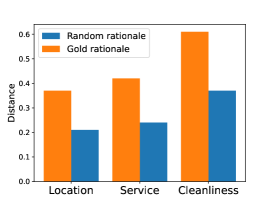
Figure 2. Average distance between rationales from positive reviews and rationales from negative reviews. Orange bars show average distance between human-annotated gold rationales from positive reviews and counterparts from negative reviews. Blue bars show average distance between randomly selected rationales from positive reviews and counterparts from negative reviews. The details are in Appendix A.3.

To demystify the correlation between degeneration and Lipschitz continuity of the predictor, without losing generality, we consider the binary classification problem such as sentiment analysis. Let $X_{i}$ and $X_{j}$ be two input texts with different classification labels: $Y_{i}=0$ (negative) and $Y_{j}=1$ (positive). $Z_{i}=f_{G}(X_{i})$ and $Z_{j}=f_{G}(X_{j})$ are two rationale candidates sampled from $X_{i}$ and $X_{j}$, respectively. We denote $\epsilon_{i}=f_{P}(Z_{i})-0$ and $\epsilon_{j}=1-f_{P}(Z_{j})$ as the discrepancies between their predictions and the true labels, and a smaller discrepancy indicates higher confidence of a prediction. $d(Z_{i},Z_{j})$ is the semantic distance between $Z_{i}$ and $Z_{j}$.

4.1. Distance Properties of Rationales

Intuitively, if $Z_{i}$ and $Z_{j}$ are uninformative rationale candidates with no sentiment tendency, then their semantic distance $d(Z_{i},Z_{j})$ is generally small, and if $Z_{i}$ and $Z_{j}$ are informative rationales with clear sentiment tendency opposite to each other, then their semantic distance $d(Z_{i},Z_{j})$ is relatively larger. The above observation is supported by the practical experimental analyses in Figure 2. The dataset is a multi-aspect classification dastset Hotel Reviews (Wang et al., 2010). Each aspect is calculated independently. More details of the experimental setup are in Appendix A.3. The results show that if $Z_{i}$ and $Z_{j}$ are randomly selected (i.e., uninformative candidates), their average distance between each other is much smaller than those of human-annotated informative rationales under a specific distance metric defined in Appendix A.3. For rigorous quantitative analysis, we quantify the qualitative intuition with an assumption:

Assumption 1.

Given any two rationale candidates $Z_{i}$ and $Z_{j}$ that are selected from the inputting texts $X_{i}$ and $X_{j}$ with label $Y_{i}=0$ and $Y_{j}=1$, an arbitrary tolerable error probability $P_{te}$ and a distance metric $d$, there exists a threshold $\delta_{p}$ corresponding to $P_{te}$ such that

(6) $$\text{if}\ d(Z_{i},Z_{j})\geq\delta_{p},\ \text{then}\ \tilde{p}(Z_{i},Z_{j})\leq P_{te},$$

where $\tilde{p}(Z_{i},Z_{j})$ denotes the probability that $Z_{i}$ and $Z_{j}$ are not both informative.

4.2. Small Lipschitz Constant Leading to High Likelihood of Informative Candidates

We first qualitatively show that the generator is highly inclined to select informative rationales when the predictor is well trained and its Lipschitz constant is small, which is based on the intuition of the experiment of Figure 2 and does not involve Assumption 1. Then, we formally quantify it in Theorem 1 based on Assumption 1.

Concretizing Equation 5 into the predictor with the rationale candidate set $\mathcal{Z}$, and if the prediction error is small (i.e., $\epsilon_{i},\epsilon_{j}\leq 0.5$), the corresponding Lipschitz constant of the predictor is

(7) $$L_{c}= \mathop{\sup}_{Z_{i},Z_{j}\in\mathcal{Z}}\frac{|f_{P}(Z_{i})-f_{P}(Z_{j})|}{d(Z_{i},Z_{j})}$$

$$= \mathop{\sup}_{Z_{i},Z_{j}\in\mathcal{Z}}\frac{|(\epsilon_{i}+0)-(1-\epsilon_{j})|}{d(Z_{i},Z_{j})}$$

$$= \mathop{\sup}_{Z_{i},Z_{j}\in\mathcal{Z}}\frac{1-\epsilon_{j}-\epsilon_{i}}{d(Z_{i},Z_{j})}.$$

$L_{c}$ is the supremum, so we have $L_{c}\geq\frac{1-\epsilon_{j}-\epsilon_{i}}{d(Z_{i},Z_{j})}$, and we further get

(8) $$d(Z_{i},Z_{j})\geq\frac{1-\epsilon_{j}-\epsilon_{i}}{L_{c}}.$$

When the RNP model gives high-confidence predictions close to the true labels, $\frac{1-\epsilon_{j}-\epsilon_{i}}{L_{c}}$ can be seen as a lower bound of $d(Z_{i},Z_{j})$. Since informative candidates containing clear sentiment tendencies tend to have a greater distance between them than those uninformative ones, if $L_{c}$ is small enough, the predictor can make the right predictions (i.e., low $\epsilon_{i},\epsilon_{j}$) with only informative candidates which have large $d(Z_{i},Z_{j})$, forcing the generator to select these candidates as rationales. Quantitatively, we have:

Theorem 1.

Under Assumption 1, given any two rationale candidates $Z_{i}$ and $Z_{j}$ that are selected from the inputting texts $X_{i}$ and $X_{j}$ with label $Y_{i}=0$ and $Y_{j}=1$, if the predictor makes correct predictions (i.e., $\epsilon_{i},\epsilon_{j}\leq 0.5$) and its Lipschitz constant is small (i.e., $L_{c}\leq\frac{1-\epsilon_{j}-\epsilon_{i}}{\delta_{p}}$), then the probability that both $Z_{i}$ and $Z_{j}$ are informative rationales is at least $1-P_{te}$.

The proof is in Appendix C.1. As a consequence, constraining the Lipschitz constant of the predictor to be small can ease the degeneration problem where the predictor makes the right predictions with uninformative rationales.

Verification with spectral normalization. There have been some existing methods such as weight clipping (Arjovsky et al., 2017b) and spectral normalization (Miyato et al., 2018), which can restrict the Lipschitz constant with some manually selected cutoff values. To verify the theoretical result that small Lipschitz constant improving the rationale quality, we conduct an experiment by simply applying the widely used spectral normalization (Miyato et al., 2018) to RNP’s predictor’s linear layer for restricting the Lipschitz constant. Figure LABEL:fig:RNP_SN(a) shows that on all three independently trained datasets the rationale quality is significantly improved when the spectral normalization is applied, which demonstrates the effectiveness of restricting Lipschitz constant.

However, the manually selected cutoff values are not flexible and often limit the model capacity (Wu et al., 2021; Zhang et al., 2022). In fact, different datasets need different values of the Lipschitz constant to maintain the model capacity in prediction. Figure LABEL:fig:RNP_SN(b) shows that spectral normalization hurts the prediction performance. Besides, these existing methods are also hard to be applied to complex network structures, such as RNN (including GRU and LSTM) and Transformer, which have multiple sets of parameters playing different roles that should not be treat equally. Gradient penalty (Gulrajani et al., 2017), which is another method of restricting the Lipschitz constant used in GANs, also fails because its objective function is not suitable for classification tasks and it is hard to create meaningful mixed data points due to the different lengths of input texts.

Instead of roughly truncating the Lipschitz constant, we use a simple method to guide the predictor to obtain an adaptively small Lipschitz constant without affecting its capacity, which can not only be applied to the RNN or Transformer based predictor in order to ease degeneration and improve rationale quality but also can maintain the good prediction performance.

5. Decoupled Rationalization with Asymmetric Learning Rates

5.1. Correlation Between Learning Rates and the Lipschitz Constant

Qualitative analysis. Back to Equation 8, we have

(9) $$\epsilon_{i}+\epsilon_{j}\geq 1-d(f_{G}(X_{i}),f_{G}(X_{j}))\cdot L_{c},$$

where $L_{c}$ is related to $\theta_{p}$ and $d(f_{G}(X_{i}),f_{G}(X_{j}))$ is related to $\theta_{g}$. The goal of Equation 2 is to minimize the prediction discrepancies $\epsilon_{i}$ and $\epsilon_{j}$, which can be obtained by increasing the product $d(f_{G}(X_{i}),f_{G}(X_{j}))\cdot L_{c}$ by tuning $\theta_{g}$ and $\theta_{p}$. By tuning $\theta_{g}$, the generator tries to find rationales that get large distance between different categories so as to reduce the prediction discrepancies with greater $d(f_{G}(X_{i}),f_{G}(X_{j}))$. For the predictor, $L_{c}$ will be increased when it tunes $\theta_{p}$ to get lower $\epsilon$ on given rationale candidates, which is also reflected in Equation 7. In short, both $d(f_{G}(X_{i}),f_{G}(X_{j}))$ and $L_{c}$ tends to grow during training, but we want $L_{c}$ to be restricted to a small extent for better rationale quality. So, if we slow down the predictor and speed up the generator, chances are that the increase in the product comes mainly from increasing $d(f_{G}(X_{i}),f_{G}(X_{j}))$ by selecting rationales with clear sentiment tendencies rather than increasing $L_{c}$ by overfitting the predictor quickly.

Empirical support. To show this, we carry out a motivation experiment with different learning rates for the predictor by setting the learning rate of the generator to be fixed at $\alpha_{g}=0.0001$, and the learning rate of the predictor as $\alpha_{p}=\lambda\alpha_{g}$ ranging from $0.001$ ($\lambda=10$) to $0.0000067$ ($\lambda=1/15$). The Lipschitz constant is approximated by $\mathop{\max}\limits_{Z\in\mathcal{Z}_{train}}||\nabla_{Z}f_{P}(Z)||_{2}$ (Paulavičius and Žilinskas, 2006) (see Appendix A.4). The results are shown in Figure LABEL:fig:lip_with_different_pred_lr (a). We can find that Lipschitz constant of the predictor exhibits explosive growth when $\alpha_{p}$ is higher than $\alpha_{g}$ (i.e., $\lambda>1$). And the Lipschitz constant are constrained to much smaller values when $\alpha_{p}$ is lower than $\alpha_{g}$ (i.e., $\lambda<1$).

5.2. The Proposed Method

Although we conclude that small learning rate brings benefits for training RNP models, it is still hard to determine the optimal value. In fact, there exists a trade-off between the Lipschitz constant and the training speed where small learning rate will restrict the Lipschitz constant but will also slow down the training speed. Inspired by the rationale sparsity constraint used in Equation 3, we in this paper propose a simple heuristic but empirically effective method of setting $\lambda$ for the learning rate of predictor such that the Lipschitz constant is reduced while still maintaining the training speed:

(10) $$\lambda=\frac{||M||_{1}}{l},$$

where $||M||_{1}$ is the number of selected tokens and $l$ is the length of the full text. The generator can access the full input text, but the predictor can only get incomplete information contained in the rationale as a subset, which is only on average a proportion of $\frac{||M||_{1}}{l}$ of the full input text, so it seems reasonable to slow down the predictor by this ratio in order to make its decision more cautiously with incomplete information. We have also conducted experiments with $\lambda$ ranging form $5$ to $1/15$ in Section 6.

In Figure LABEL:fig:lip_with_different_pred_lr (b), we compare the approximate Lipschitz constants of the well trained predictors between RNP ($\lambda=1$) and our model using asymmetric and adaptive learning rates ($\lambda=\frac{||M||_{1}}{l}$). We find that in all six aspects of the two datasets, our method gets much smaller Lipschitz constants compared to the vanilla RNP. The results in Figure LABEL:fig:lip_with_different_pred_lr (b) are also consistent with the rationale quality results of $F1$ scores in Table 4(a) and Table 4(b), in which our method also gets higher $F1$ scores compared to the vanilla RNP in all six aspects. Again, this reflects that Lipschitz continuity does play an important role in the quality of the selected rationales.

Table 2. Statistics of datasets used in this paper

Datasets		Train		Dev		Annotation
		Pos	Neg	Pos	Neg	Pos	Neg	S
Beer	Appearance	16891	16891	6628	2103	923	13	18.5
	Aroma	15169	15169	6579	2218	848	29	15.6
	Palate	13652	13652	6740	2000	785	20	12.4
Hotel	Location	7236	7236	906	906	104	96	8.5
	Service	50742	50742	6344	6344	101	99	11.5
	Cleanliness	75049	75049	9382	9382	99	101	8.9

6. Experiments

Table 3. Results on two standard benchmarks: BeerAdvocate and HotelReview datasets. Each aspect is trained independently. $``*"$: results obtained from the paper of FR (Liu et al., 2022). $``$re-$"$: our reimplemented methods. The underlined numbers are the second best results.

Methods	Appearance					Aroma					Palate
	S	Acc	P	R	F1	S	Acc	P	R	F1	S	Acc	P	R	F1
DMR*	18.2	-	71.1	70.2	70.7	15.4	-	59.8	58.9	59.3	11.9	-	53.2	50.9	52.0
A2R*	18.4	83.9	72.7	72.3	72.5	15.4	86.3	63.6	62.9	63.2	12.4	81.2	57.4	57.3	57.4
FR*	18.4	87.2	82.9	82.6	82.8	15.0	88.6	74.7	72.1	73.4	12.1	89.7	67.8	66.2	67.0
re-RNP	18.2	83.3	73.8	72.7	73.2	16.0	85.2	64.1	65.9	64.9	13.0	85.2	60.1	63.1	61.5
DR(ours)	18.6	85.3	84.3	84.8	84.5	15.6	87.2	77.2	77.5	77.3	13.3	85.7	65.1	69.8	67.4

(a) BeerAdvocate

Methods	Location					Service					Cleanliness
	S	Acc	P	R	F1	S	Acc	P	R	F1	S	Acc	P	R	F1
DMR*	10.7	-	47.5	60.1	53.1	11.6	-	43.0	43.6	43.3	10.3	-	31.4	36.4	33.7
A2R*	8.5	87.5	43.1	43.2	43.1	11.4	96.5	37.3	37.2	37.2	8.9	94.5	33.2	33.3	33.3
FR*	9.0	93.5	55.5	58.9	57.1	11.5	94.5	44.8	44.7	44.8	11.0	96.0	34.9	43.4	38.7
RNP*	8.8	97.5	46.2	48.2	47.1	11.0	97.5	34.2	32.9	33.5	10.5	96.0	29.1	34.6	31.6
DR(ours)	9.6	96.5	53.6	60.9	57.0	11.5	96.0	47.1	47.4	47.2	10.0	97.0	39.3	44.3	41.8

(b) HotelReview

6.1. Datasets

Following Huang et al. (2021) and Liu et al. (2022), we consider two widely used datasets for rationalization tasks. BeerAdvocate (McAuley et al., 2012) is a multi-aspect sentiment prediction dataset on reviewing beers. Following previous works (Chang et al., 2019; Huang et al., 2021; Yu et al., 2021; Liu et al., 2022), we use the subsets decorrelated by Lei et al. (2016) and binarize the labels as Bao et al. (2018) did. HotelReview (Wang et al., 2010) is another multi-aspect sentiment prediction dataset on reviewing hotels. The dataset contains reviews of hotels from three aspects including location, cleanliness, and service. Each review has a rating on a scale of 0-5 stars. We binarize the labels as (Bao et al., 2018) did. Both datasets contain human-annotated rationales on the annotation (test) set only. The statistics of the datasets are in Table 2. $Pos$ and $Neg$ denote the number of positive and negative examples in each set. $S$ denotes the average percentage of tokens in human-annotated rationales to the whole texts.

We preprocess both datasets in the same way as FR (Liu et al., 2022) for a fair comparison and the details are in Appendix A.1.

6.2. Baselines and Implementation Details

The main baseline for direct comparison is the original cooperative rationalization framework RNP (Lei et al., 2016), as RNP and our DR match in selection granularity, optimization algorithm and model architecture, which helps us to focus on our claims rather than some potential unknown mechanisms. To show the competitiveness of our method, we also include several recently published models that achieve state-of-the-art results: DMR (Huang et al., 2021), A2R (Yu et al., 2021) and FR (Liu et al., 2022), all of which have been discussed in detail in Section 2.

Experiments in recent works show that it is still a challenging task to finetune large pretrained language models on the RNP cooperative framework (Chen et al., 2022; Liu et al., 2022). For example, Table 7 shows that several improved rationalization methods fail to find the true rationales when using pretrained models (e.g., ELECTRA-small (Clark et al., 2020) and BERT-base (Devlin et al., 2019)) as the encoders of the players. To make a fair comparison, we take the same setting as previous works do (Huang et al., 2021; Yu et al., 2021; Liu et al., 2022). We use one-layer 200-dimension bi-directional gated recurrent units (GRUs) (Cho et al., 2014) followed by one linear layer for each of the players, and the word embedding is 100-dimension Glove (Pennington et al., 2014). The optimizer is Adam (Kingma and Ba, 2015). The reparameterization trick for binarized sampling is Gumbel-softmax (Jang et al., 2017; Bao et al., 2018), which is also the same as FR. We take the results when the development set gets the highest prediction accuracy. To show the competitiveness of our DR, we further conduct some experiments with pretrained language models as a supplement to the main experiments.

Metrics. Following previous works (Huang et al., 2021; Yu et al., 2021; Liu et al., 2022), we focus on the rationale quality, which is measured by the overlap between the model-selected tokens and human-annotated tokens. $P,R,F1$ indicate the precision, recall, and F1 score, respectively. $S$ indicates the average percentage (sparsity) of selected tokens to the whole texts. $Acc$ indicates the predictive accuracy.

6.3. Results

Comparison with state-of-the-arts. Table 4(a) and  4(b) show the main results compared to previous methods on two standard benchmarks. In terms of $F1$ score, our approach outperforms the best available methods in five out of six aspects of the two datasets. In particular, as compared to our direct baseline RNP, we get improvements of more than $10\%$ in terms of F1 score in four aspects (i.e., Appearance, Aroma, Service, Cleanliness). The improvement shows that the heuristic of setting $\lambda$ in our DR is a very strong one. Figure LABEL:fig:lip_with_different_pred_lr (b) shows the Lipschitz constants of well-trained RNP and DR on different datasets. Table 9 shows some visualized examples of rationales from RNP and our DR. We also provide some failure cases of our DR in Appendix B.2 to pave the way for future work.

Table 4. Results of methods with low sparsity on BeerAdvocate. $``*"$ and $``**"$: results obtained from the papers of CAR (Chang et al., 2019) and DMR (Huang et al., 2021), respectively.

Methods	Appearance					Aroma					Plate
	S	Acc	P	R	F1	S	Acc	P	R	F1	S	Acc	P	R	F1
RNP∗	11.9	-	72.0	46.1	56.2	10.7	-	70.5	48.3	57.3	10.0	-	53.1	42.8	47.5
CAR∗	11.9	-	76.2	49.3	59.9	10.3	-	50.3	33.3	40.1	10.2	-	56.6	46.2	50.9
DMR∗∗	11.7	-	83.6	52.8	64.7	11.7	-	63.1	47.6	54.3	10.7	-	55.8	48.1	51.7
DR(ours)	11.9	81.4	86.8	55.9	68.0	11.2	80.5	70.8	57.1	63.2	10.5	81.4	71.22	60.2	65.3

Results with different $\lambda$ values. Since we do not have a rigorous theoretical analysis for choosing the best $\lambda$, in Figure 5 we run the experiments with a wide range of values of $\lambda$ to verify our claim that lowering the learning rate of predictor can alleviate degeneration. We take five different values of $\lambda$: 1/15, 1/10, 1/5, 1, 5 (shown along the vertical axis) and five different learning rates for the generator ranging from $0.0001$ to $0.001$ (with corresponding ratios shown along the horizontal axis). The values in the cells are $F1$ scores reflecting rationale quality. The experimental results demonstrate that, given a vanilla RNP model with the setting of $\lambda=1$, making the learning rate of its predictor lower than that of its generator, i.e., lowering $\lambda$ to some value smaller than 1, can always get rationales much better than the original RNP. And it seems that the results are not too sensitive to the value of $\lambda$ as long as the value of $\lambda$ is smaller than 1. We also compare the results of our method DR ($\lambda=\frac{||M||_{1}}{l}$) shown in Table 4(a) with the corresponding best results in Figure 5, and find that our heuristic setting of $\lambda$ in Equation 10 is a reasonably good option that is empirically close to the optimal solution.

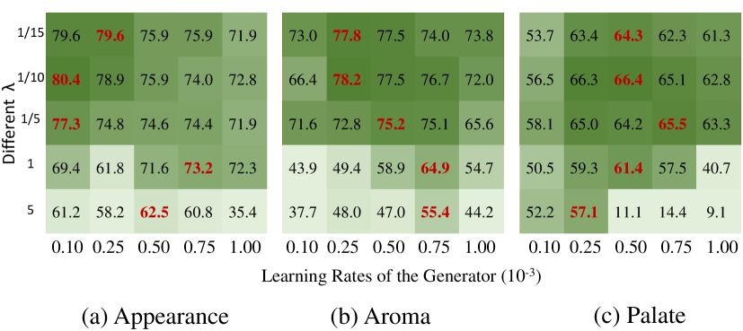
Figure 5. Results with different values of $\lambda$ in the three aspects of BeerAdvocate. The values in these cells are F1 scores.

Comparison with baselines in low sparsity. To show the robustness of our method, we also conduct an experiment where the sparsity of selected rationales is very low, which is the same as the sparsity used in CAR (Chang et al., 2019) and DMR (Huang et al., 2021). The results are shown in Table 4. We still significantly outperform the baselines.

Inducing degeneration with skewed predictor. To show that even if the predictor overfits to trivial patterns, our DR can still escape from degeneration, we conduct the same synthetic experiment that gives the predictor very poor initialization and deliberately induces degeneration as Yu et al. (2021) did. We first pretrain the predictor separately using only the first sentence of input text, and then cooperatively train the predictor initialized with the pretrained parameters and the generator randomly initialized using normal input text. “skew$k$” means that the predictor is pre-trained for $k$ epochs. For a fair comparison, we keep the pre-training process the same as in A2R: we use a batch-size of 500 and a learning rate of 0.001. More details of this experiment can be found in Appendix B.1.

The results are shown in Table 5. The results of RNP and A2R are obtained from A2R (Yu et al., 2021), and results of FR are also copied from its original paper (Liu et al., 2022). For all the settings, we outperform all the three methods. Especially, for the relatively easy task on Aroma, the performance of DR is hardly affected by this poor initialization. And for the relatively hard task on Palate, it is only slightly affected, while RNP and A2R can hardly work and FR is also significantly affected. It can be concluded that DR is much more robust than the other two methods in this situation.

Inducing degeneration with skewed generator. It is a synthetic experiment with a special initialization that induces degeneration from the perspective of skewed generator, which is designed by Liu et al. (2022). We pretrain the generator separately using the text classification label as the mask label of the first token. In other words, for texts of class 1, we force the generator to select the first token, and for texts of class 0, we force the generator not to select the first token. So, the generator learns the category implicitly by whether the first token is chosen and the predictor only needs to learn this position information to make a correct prediction.

All the hyperparameters are the same as those of the best results of the corresponding models in Table 4(a). We use Beer-Palate because A2R and FR show that Palate is harder than other aspects. $k$ in “skew$k$” denotes the threshold of the skew: we pretrain the generator as a special classifier of the first token for a few epochs until its prediction accuracy is higher than $k$. Since the accuracy increases rapidly in the first a few epochs, obtaining a model that precisely achieves the pre-defined accuracy is almost impossible. So, we use “$Pre\_acc$” to denote the actual prediction accuracy of the generator-classifier when the pre-training process stops. Higher “$Pre\_acc$” means easier to degenerate.

The results are shown in Table 6. In this case, RNP fails to find the human-annotated rationales and FR is also significantly affected when the skew degree is high. While our DR is much less affected, which shows the robustness of our DR under this case.

Table 5. Results of skewed predictor that induces degeneration on BeerAdvocate. $``*"$ and $``**"$: results obtained from the papers of A2R (Yu et al., 2021) and FR (Liu et al., 2022), respectively.

Aspect	Setting	RNP*				A2R*				FR**				DR(ours)
		Acc	P	R	F1	Acc	P	R	F1	Acc	P	R	F1	Acc	P	R	F1
Aroma	skew10	82.6	68.5	63.7	61.5	84.5	78.3	70.6	69.2	87.1	73.9	71.7	72.8	85.0	77.3	75.7	76.5
	skew15	80.4	54.5	51.6	49.3	81.8	58.1	53.3	51.7	86.7	71.3	68.0	69.6	85.4	76.1	77.2	76.6
	skew20	76.8	10.8	14.1	11.0	80.0	51.7	47.9	46.3	85.5	72.3	69.0	70.6	85.5	77.3	76.2	76.8
Palate	skew10	77.3	5.6	7.4	5.5	82.8	50.3	48.0	45.5	75.8	54.6	61.2	57.7	85.8	67.7	68.6	68.2
	skew15	77.1	1.2	2.5	1.3	80.9	30.2	29.9	27.7	81.7	51.0	58.4	54.5	83.9	66.3	66.7	66.5
	skew20	75.6	0.4	1.4	0.6	76.7	0.4	1.6	0.6	83.1	48.0	58.9	52.9	85.0	59.4	62.6	61.0

Table 6. Results of skewed generator that induces degeneration in the Palate aspect of BeerAdvocate. $``*"$: results obtained from the paper of FR.

Setting	RNP*						FR*						DR(ours)
	Pre_acc	S	Acc	R	R	F1	Pre_acc	S	Acc	P	R	F1	Pre_acc	S	Acc	P	R	F1
skew65.0	66.6	14.0	83.9	40.3	45.4	42.7	66.3	14.2	81.5	59.5	67.9	63.4	68.5	12.5	81.9	60.9	61.1	61.0
skew70.0	71.3	14.7	84.1	10.0	11.7	10.8	70.8	14.1	88.3	54.7	62.1	58.1	70.3	12.8	84.2	61.8	63.6	62.6
skew75.0	75.5	14.7	87.6	8.1	9.6	8.8	75.6	13.1	84.8	49.7	52.2	51.0	75.5	12.8	81.8	58.8	60.6	59.7

Experiments with pretrained language models. In the field of rationalization, researchers generally focus on frameworks of the models and the methodology rather than engineering SOTA. The methods most related to our work do not use BERT or other pre-trained encoders (Chang et al., 2019, 2020; Huang et al., 2021; Yu et al., 2019, 2021; Liu et al., 2022). Experiments in some recent work (Chen et al., 2022; Liu et al., 2022) indicate that there are some unknown obstacles making it hard to finetune large pretrained models on the self-explaining rationalization framework. For example, Table 7 shows that two improved rationalization methods (VIB (Paranjape et al., 2020) and SPECTRA (Miyato et al., 2018)) and the latest published FR all fail to find the informative rationales when replacing GRUs with pretrained language models. To eliminate potential factors that could lead to an unfair comparison, we adopt the most widely used GRUs as the encoders in our main experiments, which can help us focus more on our claims themselves rather than unknown tricks.

But to show the competitiveness of our DR, we also provide some experiments with pretrained language models as the supplement. Due to limited GPU resources, we adopt the relatively small ELECTRA-small (Clark et al., 2020) in all three aspects of BeerAdvocate and the relatively large BERT-base (Devlin et al., 2019) in the Appearance aspect. We compare our DR with the latest SOTA FR (Liu et al., 2022). The results with BERT-base are shown in Table 7 and the results with ELECTRA-small are shown in Table 8. Although DR sometimes still performs worse than the models with GRUs, it makes a great progress in this line of research as compared to the previous methods like VIB (Paranjape et al., 2020), SPECTRA (Miyato et al., 2018) and FR (Liu et al., 2022). Although we still do not get as good rationales as using GRUs, we are making great strides compared to previous methods.

Table 7. The rationale quality (F1 score) of models trained with different encoders. $``$*$"$: The results of VIB (Paranjape et al., 2020) and SPECTRA (Miyato et al., 2018) are from Chen et al. (2022). $``$**$"$: The results of RNP and FR (Liu et al., 2022) are from Liu et al. (2022). The dataset is Beer-Appearance.

Method	GRU	ELECTRA	BERT
VIB*	-	-	20.5
SPECTRA*	-	-	28.6
RNP**	72.3	13.7	14.7
FR**	82.8	14.6	29.8
DR(ours)	84.5	87.2	85.0

Table 8. Results of methods using pretrained ELECTRA as the encoder. The dataset is BeerAdvocate.

Methods	Appearance					Aroma					Plate
	S	Acc	P	R	F1	S	Acc	P	R	F1	S	Acc	P	R	F1
FR	16.3	86.5	19.1	17.0	18.0	14.8	85.9	58.6	54.8	56.7	11.2	78.0	12.0	10.7	11.3
DR(ours)	17.4	93.0	89.4	85.0	87.2	14.5	89.5	79.2	72.4	75.7	12.5	88.9	61.1	60.5	60.8

Table 9. Examples of generated rationales. Human-annotated rationales are underlined. Rationales from RNP and DR are highlighted in red and blue respectively.

RNP	DR(ours)
Aspect: Beer-Aroma	Aspect: Beer-Aroma
Label: Positive, Pred: Positive	Label: Positive, Pred: Positive
Text: this beer poured a hypnotically deep amber color almost as though it wanted to be an american brown . near white head that faded quickly way darker than i was expecting .   hops nose but not nearly as aggressive as most ipas . so far not what i think of an ipa . the taste is malty at the very beginning then followed by a punch of hops that hits you right in the back of the jaw . exactly what it should be . the finish is especially bitter and hoppy . the mouthfeel is good ; moderate carbonation and smooth . poignant and bitter in a notable way . a strange ipa but an outstanding one .	Text: this beer poured a hypnotically deep amber color almost as though it wanted to be an american brown . near white head that faded quickly way darker than i was expecting .   hops nose but not nearly as aggressive as most ipas . so far not what i think of an ipa . the taste is malty at the very beginning then followed by a punch of hops that hits you right in the back of the jaw . exactly what it should be . the finish is especially bitter and hoppy . the mouthfeel is good ; moderate carbonation and smooth . poignant and bitter in a notable way . a strange ipa but an outstanding one .
Aspect: Beer-Palate	Aspect: Beer-Palate
Label: Positive, Pred: Positive	Label: Positive, Pred: Positive
Text: on tap at pope in philly pours a completely clouded golden color with some yellow hues . thick , frothy white head retains well on top , fading into some layers of film with some rings of lacing on the glass spicy and citrusy on the nose . some lemon peel and cracked pepper with a hint of orange sweetness . barely any alcohol with some soft brett funk and yeast splash of floral hops up front with peppery spice . some herbal notes followed by citrus juiciness and lemon peel . a little sweet in the middle from the fruit . hints of [unknown] funk and belgian yeast , but not quite tart . finishes a little spicy   medium body , higher carbonation , refreshing and tingly on the palate . a solid saison , although i was hoping for more brett presence .	Text: on tap at pope in philly pours a completely clouded golden color with some yellow hues . thick , frothy white head retains well on top , fading into some layers of film with some rings of lacing on the glass spicy and citrusy on the nose . some lemon peel and cracked pepper with a hint of orange sweetness . barely any alcohol with some soft brett funk and yeast splash of floral hops up front with peppery spice . some herbal notes followed by citrus juiciness and lemon peel . a little sweet in the middle from the fruit . hints of [unknown] funk and belgian yeast , but not quite tart . finishes a little spicy  medium body , higher carbonation , refreshing and tingly on the palate . a solid saison , although i was hoping for more brett presence .

Time efficiency and overfitting. At first glance, it seems that lowering the learning rate of the predictor might slow down the convergence of the training process. However, the experiments show that convergence of our model is not slowed down at all. Figure 6 (a) shows the evolution of the $F1$ scores over the training epochs. All the settings are the same except that we use $\lambda=\frac{||M||_{1}}{l}$ while RNP uses $\lambda=1$. Figure 6 (b) shows that the training accuracy of RNP grows fast in the beginning when limited rationales have been sampled by the generator, and reflects that the predictor is trying to overfit to these randomly sampled rationales. Figure 6 (c) shows that, although RNP gets a very high accuracy in the training dataset, it does not get accuracy higher than our method in the development dateset, and also indicates the fact of overfitting. The prediction loss in Figure 6 (d) reflects a similar phenomenon.

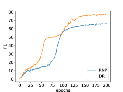
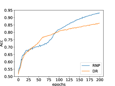
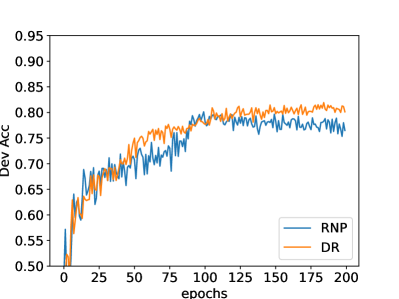
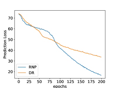
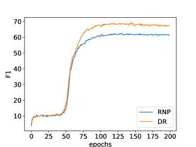
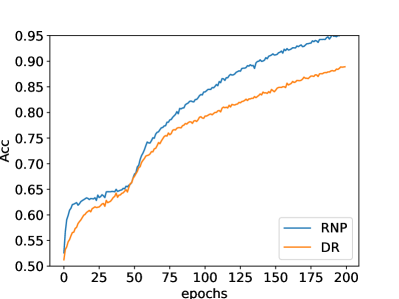
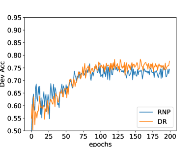
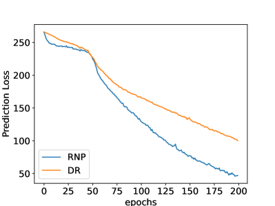
Figure 7. The training process on Beer-Aroma (a,b,c,d) and Beer-Palate (e,f,g,h).

We show more results about the time efficiency and overfitting phenomenon on Beer-Aroma and Beer-Palate in Figure 7 of the Appendix. We see that we have better or close time efficiency compared to Vanilla RNP and we always get much less overfitting.

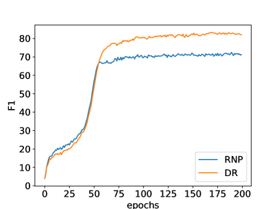
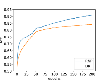
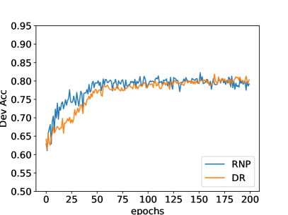
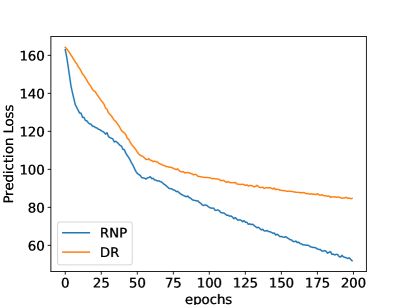
Figure 6. The training process of RNP and our DR on Beer-Appearance.

7. Conclusion and future work

In this paper, we first bridge the degeneration in cooperative rationalization with the predictor’s Lipschitz continuity. Then we analyze the two players’ coordination so as to propose a simple but effective method to guide the predictor to converge with good Lipschitz continuity. Compared to existing methods, we do not impose complex regularizations or rigid restrictions on the model parameters of the RNP framework, so that the predictive capacity is not affected. Although there is no rigorous theoretical analysis on how to choose the best $\lambda$, the method to obtain good Lipschitz continuity in this paper is simple but empirically effective, which paves the way for future research. Other methods that can help to obtain networks with good Lipschitz continuity can be also explored to promote rationalization research in the future.

Given the versatility of the self-explaining rationalization framework, our proposed methods show significant potential for application across diverse fields such as multi-aspect recommender systems (Deng et al., 2023) and computer vision (Yuan et al., 2022).

8. Limitations

One limitation may be that how to apply this simple learning rate strategy to other variants of this type of two-player rationalization requires further exploration, which we leave as future work.

Another limitation is that the obstacles in utilizing powerful pretrained language models under the rationalization framework remain mysterious. Though we have made some progress in this direction, the empirical results with pretrained models don’t show significant improvements as compared to those with GRUs. Further efforts should be made in the future. However, it’s somewhat beyond the scope of this paper, and we leave it as the future work.

Appendix A Experimental Setup

A.1. Datasets

BeerAdvacate Following Chang et al. (2019); Huang et al. (2021); Yu et al. (2021), we consider a classification setting by treating reviews with ratings $\leq$ 0.4 as negative and $\geq$ 0.6 as positive. Then we randomly select examples from the original training set to construct a balanced set.

Hotel Reviews Similar to BeerAdvacate, we treat reviews with ratings $<$ 3 as negative and $>$ 3 as positive.

A.2. Implementation details

We reimplement RNP with updated short and coherent regularizers (Equation 3) and reparameterization trick (gumbel-softmax) to make RNP and our DR match in all the details except that DR uses asymmetric learning rates. The early stop is conducted according to the predictive accuracy on the development set.

A.3. The setup of Figure 2

We first give the formal definition of the properties that a distance metric should have:

Definition 0.

We call $d$ is a distance metric if and only if it satisfies the four basic properties:

(11) $$d(A,B)\geq 0,$$

$$d(A,B)=0\ \text{iff}\ A=B,$$

$$d(A,B)=d(B,A),$$

$$d(A,B)\leq d(A,C)+d(B,C).$$

We denote the set of all the possible distance metric as $\mathcal{M}$.

The specific distance in Figure 2 is defined as:

Definition 0.

For two text sequences $A=a_{1:n}$, $B=b_{1:m}$, where $a_{i},b_{i}\in R^{d}$ are the word embeddings (Glove-100 in this paper). We define a distance between them as

(12) $$d_{t}(A,B)=||\frac{1}{n}\sum\limits_{i=1}^{n}a_{i}-\frac{1}{m}\sum\limits_{i=1}^{m}b_{i}||_{2},$$

where we use the average because different sentences have different lengths. It is easy to prove that this definition satisfies the four basic properties implied in Definition 1. It’s worth noting that our theoretical derivations doesn’t involve any specific distance definition, instead, they hold for any $d\in\mathcal{M}$. Definition 2 is only used in our quantitative experiments.

We uses the Hotel dataset because the Beer dataset is not balanced (see Table 2). We first randomly sample the same number of words as the human-annotated rationale (GR in Figure 2) from each text in the annotation set as the uninformative rationale (RR in Figure 2). The word vector is 100-dimension GloVe. Note that the original $Z$ is a matrix with shape $\mathcal{R}^{b\times d}$, where $b$ is the number of tokens in $Z$ and $d$ is the dimension of the word vector. $b$ varies according to different $Z$. To compute the norm, we need to unify rationales of different lengths into a vector of the same length. We first obtain the representation of a rationale by averaging the word vectors of all its words. Formally, for a rationale $Z=[z_{1},z_{2},\cdots,z_{b}]$ where $z_{i}\in\mathcal{R}^{d}$ is the $i$-th token, we represent $Z$ as a $d$-dimensional vertor by $Z=\frac{z_{1}+z_{2}+\cdots+z_{b}}{b}$. Now we get $Z\in\mathcal{R}^{d}$. Then, we obtain the centroids of the categories by averaging over the rationales in the same category. Finally, we obtain the average distance between the two categories by measuring distance between corresponding centroids with the norm of different orders.

A.4. Calculating the approximate Lipschitz constant through sampling gradient norm

As implied in (Paulavičius and Žilinskas, 2006; Weng et al., 2018), the Lipschitz constant can be calculated by the gradient norm.

Lemma 0.

If a function $f(\cdot):\mathcal{R}^{n}\xrightarrow{}\mathcal{R}^{1}$ is Lipschitz continuous on $\mathcal{X}\subset\mathcal{R}^{n}$, then, the Lipschitz constant corresponding to Equation 5 can be calculated through

(13) $$L_{c}=\mathop{\max}\limits_{X\in\mathcal{X}}{||\nabla f(X)||_{q}},\ s.t.\ \frac{1}{p}+\frac{1}{q}=1$$

where $\nabla f(X)=(\frac{\partial f(X)}{\partial x_{1}},\cdots,\frac{\partial f(X)}{\partial x_{n}})^{\top}$.

A usual setting is that $p=q=2$. Here we calculate the Lipschitz constant of the predictor whose input is a rationale and the output is a value ranging in $(0,1)$. It is intractable to calculate the maximum $||\nabla f(X)||_{p}$ because there are endless $X$, and a common practice is to approximate it by sampling (Weng et al., 2018). We use the training set to calculate $L_{c}$ because the model fits the training set better. For each full text in the whole training set, we first generate one rationale $Z$ with the generator and then calculate $\nabla f(Z)$. Note that here $\nabla f(Z)\in\mathcal{R}^{b\times d}$ is a matrix, where $b$ is the length of the rationale $Z$ which may varies across different rationales and $d$ is the dimension of the word vector. Corresponding to the distance metric of Definition 2, we take the average along the length of $Z$ and get the unified $\nabla f(Z)\in\mathcal{R}^{d}$. Then we calculate $||\nabla f(Z)||_{p}$ and take the maximum value over the entire training set as the approximate $L_{c}$. It is worth noting that although different distance metrics correspond to different calculation methods of $L_{c}$, the theoretical derivation in Section 4 doesn’t involve any specific distance metric. In fact, the theoretical conclusions hold for any $d\in\mathcal{M}$. And we believe Definition 2 is somehow reasonable and will not undermine empirical qualitative conclusions in Section 5.1.

Appendix B More results

B.1. The details of skewed predictor

The experiment was first designed by (Yu et al., 2021). It deliberately induces degeneration to verify the robustness of A2R compared to RNP. We first pretrain the predictor separately using only the first sentence of input text, and further cooperatively train the predictor initialized with the pretrained parameters and the generator randomly initialized using normal input text. In Beer Reviews, the first sentence is usually about appearance. So, the predictor will overfit to the aspect of Appearance, which is uninformative for Aroma and Palate. “skew$k$” denotes the predictor is pre-trained for $k$ epochs. To make a fair comparison, we keep the pre-training process the same as that of A2R: batch-size=500 and learning-rate=0.001.

Table 10. Some failure cases of DR. The underlined piece of the text is the human-annotated rationale. Pieces of the text in blue represent the rationales from DR.

Hotel-Cleanliness

Label: positive, Prediction: positive

Input text: my husband and i just spent two nights at the grand hotel francais , and we could not have been happier with our choice . in many ways , the hotel has exceeded our expectation : the price was within our budget , breakfast was included , and the staff was friendly , helpful and fluent in english . as other travelers have mentioned , the hotel is close to the nation metro station , which makes it easy to get around . the room size was just enough to fit two people , but we had a comfortable stay throughout . overall , the hotel lives up to its high trip advisor rating . we would love to stay here again anytime .

Beer-Aroma

Label: positive, Prediction: positive

Input text: a- amber gold with a solid two maybe even three finger head . looks absolutely delicious , i dare say it is one of the best looking beers i ’ve had . s- light citrus and hops . not a very strong aroma t-wow , the hops , citrus and pine blow out the taste buds , very tangy in taste , yet perfectly balanced , leaving a crisp dry taste to the palate . m-light and crisp feel with a nice tanginess thrown in the mix . d- could drink this all night , too bad i only have one more of this brew . notes : one of the best balanced and best tasting ipa ’s i ’ve had to date . ipa fans you have to try this one .

B.2. Failure cases

To further pave ways to gain better insights of the model and help the line of rationalization research, we also provide some failure cases of our DR in Table 10. We find that the model fails to make logical reasoning. For example, the ground truth of hotel cleanliness should be inferred from the word $``$comfortable$"$. However, our model makes judgments by selecting the rationales such as $``$breakfast $\cdots$ friendly$"$, which have little relevance to the cleanliness but are positive. We leave it as the future work.

Appendix C Theorem Proof

C.1. Proof of Theorem 1

We first copy Equation 8 here:

(14) $$d(Z_{i},Z_{j})\geq\frac{1-\epsilon_{j}-\epsilon_{i}}{L_{c}}.$$

And since we have $L_{c}\leq\frac{1-\epsilon_{j}-\epsilon_{i}}{\delta_{d}}$, we then get

(15) $$d(Z_{i},Z_{j})\geq\delta_{d},$$

which is just the left part of Equation 6. According to Assumption 1, we then have

(16) $$\tilde{p}(Z_{i},Z_{j})\leq P_{te},$$

where $\tilde{p}(Z_{i},Z_{j})$ denotes the probability that $Z_{i}$ and $Z_{j}$ are not both informative. Denoting ${p}(Z_{i},Z_{j})$ as the probability that $Z_{i}$ and $Z_{j}$ are both informative, we then have

(17) $${p}(Z_{i},Z_{j})\geq 1-P_{te}.$$

The proof of Theorem 1 is completed.

References

- (1)
- Arjovsky et al. (2017a) Martin Arjovsky, Soumith Chintala, and Léon Bottou. 2017a. Wasserstein Generative Adversarial Networks. In Proceedings of the 34th International Conference on Machine Learning (Proceedings of Machine Learning Research, Vol. 70), Doina Precup and Yee Whye Teh (Eds.). PMLR, 214–223. https://proceedings.mlr.press/v70/arjovsky17a.html
- Arjovsky et al. (2017b) Martín Arjovsky, Soumith Chintala, and Léon Bottou. 2017b. Wasserstein Generative Adversarial Networks. In Proceedings of the 34th International Conference on Machine Learning, ICML 2017, Sydney, NSW, Australia, 6-11 August 2017 (Proceedings of Machine Learning Research, Vol. 70). PMLR, 214–223. http://proceedings.mlr.press/v70/arjovsky17a.html
- Bao et al. (2018) Yujia Bao, Shiyu Chang, Mo Yu, and Regina Barzilay. 2018. Deriving Machine Attention from Human Rationales. In Proceedings of the 2018 Conference on Empirical Methods in Natural Language Processing, Brussels, Belgium, October 31 - November 4, 2018. Association for Computational Linguistics, 1903–1913. https://doi.org/10.18653/v1/d18-1216
- Bastings et al. (2019) Jasmijn Bastings, Wilker Aziz, and Ivan Titov. 2019. Interpretable Neural Predictions with Differentiable Binary Variables. In Proceedings of the 57th Conference of the Association for Computational Linguistics, ACL 2019, Florence, Italy, July 28- August 2, 2019, Volume 1: Long Papers. Association for Computational Linguistics, 2963–2977. https://doi.org/10.18653/v1/p19-1284
- Chan et al. (2022) Aaron Chan, Maziar Sanjabi, Lambert Mathias, Liang Tan, Shaoliang Nie, Xiaochang Peng, Xiang Ren, and Hamed Firooz. 2022. UNIREX: A Unified Learning Framework for Language Model Rationale Extraction. In International Conference on Machine Learning, ICML 2022, 17-23 July 2022, Baltimore, Maryland, USA (Proceedings of Machine Learning Research, Vol. 162). PMLR, 2867–2889. https://proceedings.mlr.press/v162/chan22a.html
- Chang et al. (2019) Shiyu Chang, Yang Zhang, Mo Yu, and Tommi S. Jaakkola. 2019. A Game Theoretic Approach to Class-wise Selective Rationalization. In Advances in Neural Information Processing Systems 32: Annual Conference on Neural Information Processing Systems 2019, NeurIPS 2019, December 8-14, 2019, Vancouver, BC, Canada. 10055–10065. https://proceedings.neurips.cc/paper/2019/hash/5ad742cd15633b26fdce1b80f7b39f7c-Abstract.html
- Chang et al. (2020) Shiyu Chang, Yang Zhang, Mo Yu, and Tommi S. Jaakkola. 2020. Invariant Rationalization. In Proceedings of the 37th International Conference on Machine Learning, ICML 2020, 13-18 July 2020, Virtual Event (Proceedings of Machine Learning Research, Vol. 119). PMLR, 1448–1458. http://proceedings.mlr.press/v119/chang20c.html
- Chen et al. (2022) Howard Chen, Jacqueline He, Karthik Narasimhan, and Danqi Chen. 2022. Can Rationalization Improve Robustness?. In Proceedings of the 2022 Conference of the North American Chapter of the Association for Computational Linguistics: Human Language Technologies, NAACL 2022, Seattle, WA, United States, July 10-15, 2022. Association for Computational Linguistics, 3792–3805. https://doi.org/10.18653/v1/2022.naacl-main.278
- Cho et al. (2014) Kyunghyun Cho, Bart van Merrienboer, Çaglar Gülçehre, Dzmitry Bahdanau, Fethi Bougares, Holger Schwenk, and Yoshua Bengio. 2014. Learning Phrase Representations using RNN Encoder-Decoder for Statistical Machine Translation. In Proceedings of the 2014 Conference on Empirical Methods in Natural Language Processing, EMNLP 2014, October 25-29, 2014, Doha, Qatar, A meeting of SIGDAT, a Special Interest Group of the ACL. ACL, 1724–1734. https://doi.org/10.3115/v1/d14-1179
- Clark et al. (2020) Kevin Clark, Minh-Thang Luong, Quoc V. Le, and Christopher D. Manning. 2020. ELECTRA: Pre-training Text Encoders as Discriminators Rather Than Generators. In 8th International Conference on Learning Representations, ICLR 2020, Addis Ababa, Ethiopia, April 26-30, 2020. OpenReview.net. https://openreview.net/forum?id=r1xMH1BtvB
- Deng et al. (2023) Zhiying Deng, Jianjun Li, Zhiqiang Guo, and Guohui Li. 2023. Multi-Aspect Interest Neighbor-Augmented Network for Next-Basket Recommendation. In ICASSP 2023-2023 IEEE International Conference on Acoustics, Speech and Signal Processing (ICASSP). IEEE, 1–5.
- Devlin et al. (2019) Jacob Devlin, Ming-Wei Chang, Kenton Lee, and Kristina Toutanova. 2019. BERT: Pre-training of Deep Bidirectional Transformers for Language Understanding. In Proceedings of the 2019 Conference of the North American Chapter of the Association for Computational Linguistics: Human Language Technologies, NAACL-HLT 2019, Minneapolis, MN, USA, June 2-7, 2019, Volume 1 (Long and Short Papers). Association for Computational Linguistics, 4171–4186. https://doi.org/10.18653/v1/n19-1423
- Fazlyab et al. (2019) Mahyar Fazlyab, Alexander Robey, Hamed Hassani, Manfred Morari, and George J. Pappas. 2019. Efficient and Accurate Estimation of Lipschitz Constants for Deep Neural Networks. In Advances in Neural Information Processing Systems 32: Annual Conference on Neural Information Processing Systems 2019, NeurIPS 2019, December 8-14, 2019, Vancouver, BC, Canada. 11423–11434. https://proceedings.neurips.cc/paper/2019/hash/95e1533eb1b20a97777749fb94fdb944-Abstract.html
- Fernandes et al. (2022) Patrick Fernandes, Marcos V. Treviso, Danish Pruthi, André F. T. Martins, and Graham Neubig. 2022. Learning to Scaffold: Optimizing Model Explanations for Teaching. CoRR abs/2204.10810 (2022). https://doi.org/10.48550/arXiv.2204.10810 arXiv:2204.10810
- Goodfellow et al. (2014) Ian J. Goodfellow, Jean Pouget-Abadie, Mehdi Mirza, Bing Xu, David Warde-Farley, Sherjil Ozair, Aaron C. Courville, and Yoshua Bengio. 2014. Generative Adversarial Nets. In Advances in Neural Information Processing Systems 27: Annual Conference on Neural Information Processing Systems 2014, December 8-13 2014, Montreal, Quebec, Canada. 2672–2680. https://proceedings.neurips.cc/paper/2014/hash/5ca3e9b122f61f8f06494c97b1afccf3-Abstract.html
- Gulrajani et al. (2017) Ishaan Gulrajani, Faruk Ahmed, Martín Arjovsky, Vincent Dumoulin, and Aaron C. Courville. 2017. Improved Training of Wasserstein GANs. In Advances in Neural Information Processing Systems 30: Annual Conference on Neural Information Processing Systems 2017, December 4-9, 2017, Long Beach, CA, USA, Isabelle Guyon, Ulrike von Luxburg, Samy Bengio, Hanna M. Wallach, Rob Fergus, S. V. N. Vishwanathan, and Roman Garnett (Eds.). 5767–5777. https://proceedings.neurips.cc/paper/2017/hash/892c3b1c6dccd52936e27cbd0ff683d6-Abstract.html
- Havrylov et al. (2019) Serhii Havrylov, Germán Kruszewski, and Armand Joulin. 2019. Cooperative Learning of Disjoint Syntax and Semantics. In Proceedings of the 2019 Conference of the North American Chapter of the Association for Computational Linguistics: Human Language Technologies, NAACL-HLT 2019, Minneapolis, MN, USA, June 2-7, 2019, Volume 1 (Long and Short Papers), Jill Burstein, Christy Doran, and Thamar Solorio (Eds.). Association for Computational Linguistics, 1118–1128. https://doi.org/10.18653/v1/n19-1115
- Heusel et al. (2017) Martin Heusel, Hubert Ramsauer, Thomas Unterthiner, Bernhard Nessler, and Sepp Hochreiter. 2017. GANs Trained by a Two Time-Scale Update Rule Converge to a Local Nash Equilibrium. In Advances in Neural Information Processing Systems 30: Annual Conference on Neural Information Processing Systems 2017, December 4-9, 2017, Long Beach, CA, USA. 6626–6637. https://proceedings.neurips.cc/paper/2017/hash/8a1d694707eb0fefe65871369074926d-Abstract.html
- Huang et al. (2021) Yongfeng Huang, Yujun Chen, Yulun Du, and Zhilin Yang. 2021. Distribution Matching for Rationalization. In Thirty-Fifth AAAI Conference on Artificial Intelligence, AAAI 2021, Thirty-Third Conference on Innovative Applications of Artificial Intelligence, IAAI 2021, The Eleventh Symposium on Educational Advances in Artificial Intelligence, EAAI 2021, Virtual Event, February 2-9, 2021. AAAI Press, 13090–13097. https://ojs.aaai.org/index.php/AAAI/article/view/17547
- Jain et al. (2020) Sarthak Jain, Sarah Wiegreffe, Yuval Pinter, and Byron C. Wallace. 2020. Learning to Faithfully Rationalize by Construction. In Proceedings of the 58th Annual Meeting of the Association for Computational Linguistics, ACL 2020, Online, July 5-10, 2020. Association for Computational Linguistics, 4459–4473. https://doi.org/10.18653/v1/2020.acl-main.409
- Jang et al. (2017) Eric Jang, Shixiang Gu, and Ben Poole. 2017. Categorical Reparameterization with Gumbel-Softmax. In 5th International Conference on Learning Representations, ICLR 2017, Toulon, France, April 24-26, 2017, Conference Track Proceedings. OpenReview.net. https://openreview.net/forum?id=rkE3y85ee
- Kingma and Ba (2015) Diederik P. Kingma and Jimmy Ba. 2015. Adam: A Method for Stochastic Optimization. In 3rd International Conference on Learning Representations, ICLR 2015, San Diego, CA, USA, May 7-9, 2015, Conference Track Proceedings. http://arxiv.org/abs/1412.6980
- Lei et al. (2016) Tao Lei, Regina Barzilay, and Tommi S. Jaakkola. 2016. Rationalizing Neural Predictions. In Proceedings of the 2016 Conference on Empirical Methods in Natural Language Processing, EMNLP 2016, Austin, Texas, USA, November 1-4, 2016. The Association for Computational Linguistics, 107–117. https://doi.org/10.18653/v1/d16-1011
- Liu et al. (2023) Wei Liu, Haozhao Wang, Jun Wang, Ruixuan Li, Xinyang Li, Yuankai Zhang, and Yang Qiu. 2023. MGR: Multi-generator based Rationalization. In Proceedings of the 61th Annual Meeting of the Association for Computational Linguistics (Volume 1: Long Papers). Association for Computational Linguistics, Toronto, Canada.
- Liu et al. (2022) Wei Liu, Haozhao Wang, Jun Wang, Ruixuan Li, Chao Yue, and YuanKai Zhang. 2022. FR: Folded Rationalization with a Unified Encoder. In Advances in Neural Information Processing Systems, NeurIPS 2022, Vol. 35. Curran Associates, Inc., 6954–6966. https://proceedings.neurips.cc/paper_files/paper/2022/file/2e0bd92a1d3600d4288df51ac5e6be5f-Paper-Conference.pdf
- McAuley et al. (2012) Julian J. McAuley, Jure Leskovec, and Dan Jurafsky. 2012. Learning Attitudes and Attributes from Multi-aspect Reviews. In 12th IEEE International Conference on Data Mining, ICDM 2012, Brussels, Belgium, December 10-13, 2012. IEEE Computer Society, 1020–1025. https://doi.org/10.1109/ICDM.2012.110
- Miyato et al. (2018) Takeru Miyato, Toshiki Kataoka, Masanori Koyama, and Yuichi Yoshida. 2018. Spectral Normalization for Generative Adversarial Networks. In 6th International Conference on Learning Representations, ICLR 2018, Vancouver, BC, Canada, April 30 - May 3, 2018, Conference Track Proceedings. OpenReview.net. https://openreview.net/forum?id=B1QRgziT-
- Paranjape et al. (2020) Bhargavi Paranjape, Mandar Joshi, John Thickstun, Hannaneh Hajishirzi, and Luke Zettlemoyer. 2020. An Information Bottleneck Approach for Controlling Conciseness in Rationale Extraction. In Proceedings of the 2020 Conference on Empirical Methods in Natural Language Processing, EMNLP 2020, Online, November 16-20, 2020. Association for Computational Linguistics, 1938–1952. https://doi.org/10.18653/v1/2020.emnlp-main.153
- Paulavičius and Žilinskas (2006) Remigijus Paulavičius and Julius Žilinskas. 2006. Analysis of different norms and corresponding Lipschitz constants for global optimization. Technological and Economic Development of Economy 12, 4 (2006), 301–306. http://elibrary.lt/resursai/Ziniasklaida/Aukstosios/UKIO%20TECHNOLOGINIS%20IR%20EKONOMINIS%20VYSTYMAS/2004/2006/4/8.pdf
- Pennington et al. (2014) Jeffrey Pennington, Richard Socher, and Christopher D. Manning. 2014. Glove: Global Vectors for Word Representation. In Proceedings of the 2014 Conference on Empirical Methods in Natural Language Processing, EMNLP 2014, October 25-29, 2014, Doha, Qatar, A meeting of SIGDAT, a Special Interest Group of the ACL. ACL, 1532–1543. https://doi.org/10.3115/v1/d14-1162
- Plyler et al. (2021) Mitchell Plyler, Michael Green, and Min Chi. 2021. Making a (Counterfactual) Difference One Rationale at a Time. In Advances in Neural Information Processing Systems 34: Annual Conference on Neural Information Processing Systems 2021, NeurIPS 2021, December 6-14, 2021, virtual. 28701–28713. https://proceedings.neurips.cc/paper/2021/hash/f0f800c92d191d736c4411f3b3f8ef4a-Abstract.html
- Prasad et al. (2015) H. L. Prasad, Prashanth L. A., and Shalabh Bhatnagar. 2015. Two-Timescale Algorithms for Learning Nash Equilibria in General-Sum Stochastic Games. In Proceedings of the 2015 International Conference on Autonomous Agents and Multiagent Systems, AAMAS 2015, Istanbul, Turkey, May 4-8, 2015. ACM, 1371–1379. http://dl.acm.org/citation.cfm?id=2773328
- Szegedy et al. (2014) Christian Szegedy, Wojciech Zaremba, Ilya Sutskever, Joan Bruna, Dumitru Erhan, Ian J. Goodfellow, and Rob Fergus. 2014. Intriguing properties of neural networks. In 2nd International Conference on Learning Representations, ICLR 2014, Banff, AB, Canada, April 14-16, 2014, Conference Track Proceedings, Yoshua Bengio and Yann LeCun (Eds.). http://arxiv.org/abs/1312.6199
- Virmaux and Scaman (2018) Aladin Virmaux and Kevin Scaman. 2018. Lipschitz regularity of deep neural networks: analysis and efficient estimation. In Advances in Neural Information Processing Systems 31: Annual Conference on Neural Information Processing Systems 2018, NeurIPS 2018, December 3-8, 2018, Montréal, Canada. 3839–3848. https://proceedings.neurips.cc/paper/2018/hash/d54e99a6c03704e95e6965532dec148b-Abstract.html
- Wang et al. (2010) Hongning Wang, Yue Lu, and Chengxiang Zhai. 2010. Latent aspect rating analysis on review text data: a rating regression approach. In Proceedings of the 16th ACM SIGKDD International Conference on Knowledge Discovery and Data Mining, Washington, DC, USA, July 25-28, 2010. ACM, 783–792. https://doi.org/10.1145/1835804.1835903
- Weng et al. (2018) Tsui-Wei Weng, Huan Zhang, Pin-Yu Chen, Jinfeng Yi, Dong Su, Yupeng Gao, Cho-Jui Hsieh, and Luca Daniel. 2018. Evaluating the Robustness of Neural Networks: An Extreme Value Theory Approach. In 6th International Conference on Learning Representations, ICLR 2018, Vancouver, BC, Canada, April 30 - May 3, 2018, Conference Track Proceedings. OpenReview.net. https://openreview.net/forum?id=BkUHlMZ0b
- Wu et al. (2021) Yi-Lun Wu, Hong-Han Shuai, Zhi Rui Tam, and Hong-Yu Chiu. 2021. Gradient Normalization for Generative Adversarial Networks. In 2021 IEEE/CVF International Conference on Computer Vision, ICCV 2021, Montreal, QC, Canada, October 10-17, 2021. IEEE, 6353–6362. https://doi.org/10.1109/ICCV48922.2021.00631
- Yu et al. (2019) Mo Yu, Shiyu Chang, Yang Zhang, and Tommi S. Jaakkola. 2019. Rethinking Cooperative Rationalization: Introspective Extraction and Complement Control. In Proceedings of the 2019 Conference on Empirical Methods in Natural Language Processing and the 9th International Joint Conference on Natural Language Processing, EMNLP-IJCNLP 2019, Hong Kong, China, November 3-7, 2019. Association for Computational Linguistics, 4092–4101. https://doi.org/10.18653/v1/D19-1420
- Yu et al. (2021) Mo Yu, Yang Zhang, Shiyu Chang, and Tommi S. Jaakkola. 2021. Understanding Interlocking Dynamics of Cooperative Rationalization. In Advances in Neural Information Processing Systems 34: Annual Conference on Neural Information Processing Systems 2021, NeurIPS 2021, December 6-14, 2021, virtual. 12822–12835. https://proceedings.neurips.cc/paper/2021/hash/6a711a119a8a7a9f877b5f379bfe9ea2-Abstract.html
- Yuan et al. (2022) Hao Yuan, Lei Cai, Xia Hu, Jie Wang, and Shuiwang Ji. 2022. Interpreting Image Classifiers by Generating Discrete Masks. IEEE Transactions on Pattern Analysis and Machine Intelligence 44, 4 (2022), 2019–2030. https://doi.org/10.1109/TPAMI.2020.3028783
- Zhang et al. (2022) Bohang Zhang, Du Jiang, Di He, and Liwei Wang. 2022. Rethinking Lipschitz Neural Networks and Certified Robustness: A Boolean Function Perspective. In Advances in Neural Information Processing Systems, Alice H. Oh, Alekh Agarwal, Danielle Belgrave, and Kyunghyun Cho (Eds.). https://openreview.net/forum?id=xaWO6bAY0xM
- Zhang et al. (2020) Haifeng Zhang, Weizhe Chen, Zeren Huang, Minne Li, Yaodong Yang, Weinan Zhang, and Jun Wang. 2020. Bi-Level Actor-Critic for Multi-Agent Coordination. In The Thirty-Fourth AAAI Conference on Artificial Intelligence, AAAI 2020, The Thirty-Second Innovative Applications of Artificial Intelligence Conference, IAAI 2020, The Tenth AAAI Symposium on Educational Advances in Artificial Intelligence, EAAI 2020, New York, NY, USA, February 7-12, 2020. AAAI Press, 7325–7332. https://ojs.aaai.org/index.php/AAAI/article/view/6226
- Zheng et al. (2022) Yiming Zheng, Serena Booth, Julie Shah, and Yilun Zhou. 2022. The Irrationality of Neural Rationale Models. In Proceedings of the 2nd Workshop on Trustworthy Natural Language Processing (TrustNLP 2022). Association for Computational Linguistics, Seattle, U.S.A., 64–73. https://doi.org/10.18653/v1/2022.trustnlp-1.6
- Zhou et al. (2019) Zhiming Zhou, Jiadong Liang, Yuxuan Song, Lantao Yu, Hongwei Wang, Weinan Zhang, Yong Yu, and Zhihua Zhang. 2019. Lipschitz Generative Adversarial Nets. In Proceedings of the 36th International Conference on Machine Learning (Proceedings of Machine Learning Research, Vol. 97), Kamalika Chaudhuri and Ruslan Salakhutdinov (Eds.). PMLR, 7584–7593. https://proceedings.mlr.press/v97/zhou19c.html