AI-Augmented Surveys: Leveraging Large Language Models and Surveys for Opinion Prediction

Abstract

Large language models (LLMs) that produce human-like responses have begun to revolutionize research practices in the social sciences. This paper shows how we can integrate LLMs and social surveys to accurately predict individual responses to survey questions that were not asked before. We develop a novel methodological framework to personalize LLMs by considering the meaning of survey questions derived from their text, the latent beliefs of individuals inferred from their response patterns, and the temporal contexts across different survey periods through fine-tuning LLMs with survey data. Using the General Social Survey from 1972 to 2021, we show that the fine-tuned model based on Alpaca-7b can predict individual responses to survey questions that are partially missing as well as entirely missing. The remarkable prediction capabilities allow us to fill in missing trends with high confidence and pinpoint when public attitudes changed, such as the rising support for same-sex marriage. We discuss practical constraints, socio-demographic representation, and ethical concerns regarding individual autonomy and privacy when using LLMs for opinion prediction. This study demonstrates that LLMs and surveys can mutually enhance each other’s capabilities: LLMs broaden survey potential, while surveys improve the alignment of LLMs.

Introduction

Predicting opinion trends on a range of social issues, from climate change to gay marriage, is crucial for making informed decisions, tracking social changes, and understanding the dynamics of opinion formation (Brooks and Manza, 2006; Burstein, 2003). Recently, numerous breakthroughs have been made to infer and predict people’s opinions and preferences from their written records, such as books in the past (e.g., Google Ngram), internet search patterns (e.g., Google Trend), and public sentiments in social media (e.g., Twitter, Facebook, YouTube) (Beauchamp, 2017; Grimmer et al., 2022; Moore et al., 2019; O’Connor et al., 2010; Stephens-Davidowitz, 2017). However, using digital trace data for predicting public opinion presents a substantial challenge, as these “proxy” measures cannot be deemed reliable without validating them against other “ground truth” benchmarks, like surveys (Beauchamp, 2017; Ferraro and Farmer, 1999). Even if digital trace data can closely track public opinion trends, its unobtrusive and anonymous nature prompts questions about its ability to truly represent the diverse voices of the population, particularly considering the skewed representation of demographic groups in digital traces (Cesare et al., 2018). The reliance on digital trace data, despite covering a broad spectrum of opinions, makes it hard to evenly represent the real voice of the entire population.

Surveys have long been a vital tool in academic and market research, effectively measuring and predicting public opinion, thereby offering valuable insights into societal trends. Among others, the General Social Survey (GSS) – a nationally representative survey with exceptional quality – has been widely used in sociological research tracking Americans’ opinions on various social issues and their cultural preferences since the 1970s over a half-century (Marsden et al., 2020). However, surveys face challenges associated with missing data, such as refusal, skipping of questions, and attrition (Berinsky, 2017; Couper, 2017). In the case of repeated cross-sectional, nationally representative surveys such as the GSS, most survey items are asked only once or twice. Due to resource constraints, researchers must judiciously choose which questions merit inclusion, meaning not all can be monitored over time. New questions about major social shifts could only be added to these surveys after they attracted considerable public interest, leading to a lag that limits the surveys’ effectiveness in identifying pivotal moments and understanding historical social changes. While surveys provide a precise and representative measure of public opinion, their range in capturing the full spectrum of public views over time is limited.

How can we predict a broad spectrum of public opinion in the dynamic social world without compromising on accuracy and representativeness while simultaneously addressing the limitations of digital trace and survey data? This paper investigates whether we can address these challenges by fine-tuning large language models (LLMs) to predict unmeasured public opinion in nationally representative surveys. Recent studies have already suggested the possibility of using LLMs trained on massive amounts of digital traces and text data to predict public opinion by leveraging the remarkable capability of LLMs in mimicking human responses (Aher et al., 2023; Argyle et al., 2023; Chu et al., 2023; Dillion et al., 2023; Hämäläinen et al., 2023; Horton, 2023; Jiang et al., 2022; Meta Fundamental AI Research Diplomacy Team (FAIR) et al., 2022; Schramowski et al., 2022). However, the assumption behind these attempts is that LLMs can directly simulate the population-level average responses to a survey question, presuming the high levels of alignment of LLMs with the general population. This assumption has recently been challenged (Santurkar et al., 2023), which is not surprising given well-documented biases and the skewed representation of demographic groups in the digital trace data used to train LLMs (Cesare et al., 2018). Our paper aims to go beyond these approaches that assumes one-size-fits-all LLMs designed to predict the population average. Rather, we propose a novel method to personalize and contextualize LLMs to be aligned to individual-specific, heterogeneous beliefs based on their responses to other questions in specific periods. Our study demonstrates that fine-tuning LLMs with surveys can enhance the capacity of surveys to predict public opinion by accurately predicting each survey participant’s answers to new questions over long periods of time in nationally representative surveys.

Our research also critically engages with recent debates about whether LLMs could “replace” human subjects (Grossmann et al., 2023; Dillion et al., 2023). Dillion et al (2023) claimed that LLMs may be able to replace human participants in several psychological experiments on moral judgments. However, this claim is not generalizable to many fields of the social sciences, especially survey research. While LLMs are trained on a massive amount of text data generated by humans that mirrors the opinions and behaviors of millions, we need social surveys to steer the model to reflect a particular individual’s opinions for their serious application. We also need human verification at the end to ensure that its prediction is aligned with highly dynamic and diverse human voices. In contrast to the LLMs used by Dillion et al. (2023) that did not intend to capture the dynamic nature of human attitudes across a diverse group of individuals, survey researchers are mostly interested in examining person-to-person variations as well as longitudinal opinion changes. In this paper, we will demonstrate that LLMs do not render social surveys obsolete, as they can be used for the alignment of LLMs and validation of LLMs’ outputs at the minimum. Crucially, we illustrate how LLMs can tackle the challenges of missing data in social surveys and present new opportunities for social scientists through their remarkable capability to predict the next token in a question-and-answer sequence.

To anticipate the main arguments, we first introduce the opportunities and challenges of addressing the issue of unmeasured public opinions in repeated cross-sectional, nationally representative surveys, like the GSS. Next, we propose a new methodological framework to incorporate the three most important features for opinion prediction – survey questions, individual beliefs, and survey periods while contrasting it against existing vanilla LLMs and traditional imputation models. After introducing data and methods, we evaluate how much LLMs can improve the predictability of personal and public opinion across three different types of missing data challenges in the GSS data. We further present one novel application of retrodiction based on our models’ remarkable capability to predict year-level missing opinions. Then, we investigate the performance of our models across different individuals and opinions. Finally, we discuss how developing a precise opinion prediction device driven by LLMs raises concerns over privacy, individual autonomy, and the potential for misuse (Brayne, 2020; Floridi et al., 2018).

Unmeasured Public Opinion in Survey Research

We first specify three types of challenges to be addressed by LLMs to predict unmeasured public opinion in survey research. We will introduce the nature of missing data in each case and discuss the opportunities that arise from addressing each challenge. First, fig. 1, Panel A illustrates a common situation in surveys where some respondents fail to answer or skip specific questions. It is a task that has been thoroughly investigated by traditional missing imputation models based on the assumptions of missing completely at random or missing at random (van Buuren and Groothuis-Oudshoorn, 2011; Honaker et al., 2011; Rubin, 1976). However, popular multiple imputation techniques, including Amelia and MICE, do not perform well, especially in cases of imputing responses in sparse datasets (Sengupta et al., 2023), which are increasingly common due to high attrition (e.g., online surveys) or complex designs (e.g., split-ballot design). We use the term “missing data imputation” to refer to predicting response-level missing data.

Panel B presents a scenario that arises in repeated cross-sectional surveys to study longitudinal opinion trends, where certain questions were not asked in some periods, resulting in year-level missing data. By predicting responses for the missing years, we can retrodict trends and patterns that would have emerged if the data had been collected consistently every year. For example, the question of whether same-sex couples have the right to marry one another has been asked since 2008 in the General Social Survey. How would Americans have thought about same-sex marriage in the 1970s? When did public attitudes toward same-sex marriage start to shift? Developing a device to retrodict missing responses opens an entirely new opportunity for understanding historical changes, given that survey questions addressing specific issues are often introduced only after society becomes aware of social changes concerning those issues (Behr and Iyengar, 1985; Downs, 1972; Hilgartner and Bosk, 1988). Additionally, survey designers can utilize this device for question selection since it enables them to focus on less predictable questions or those expected to shift. We use the term “retrodiction” to refer to predicting year-level missing data.

Unlike Panels A and B, where existing solutions are available, Panel C presents a scenario where the goal is to predict individuals’ responses to a question that has never been asked in the existing survey data. This unasked opinion prediction task has been proposed by recent studies employing LLMs, motivated by their abilities to generate human-like responses through in-context tuning and prompt engineering (Argyle et al., 2023; Chu et al., 2023; Jiang et al., 2022; Santurkar et al., 2023). Considering the limited number of questions that can be practically included in a survey, developing a device that predicts unasked personal opinions will offer unprecedented opportunities for social science communities, businesses, organizations, and policy-makers. For example, this device could enable the prediction of people’s preferences in market research that have never been measured in the existing survey data (DellaPosta et al., 2015; Brand et al., 2023). Or, it could allow researchers to study people’s opinions on sensitive issues without directly asking them, given that asking sensitive questions may affect response quality and non-response error (Yan, 2021). Thus, achieving high accuracy in this task suggests the potential to infinitely expand the number of variables we can predict, unlocking unparalleled opportunities. We use the term “unasked opinion prediction” to refer to predicting responses to a question without any prior survey responses about the question in the training data.

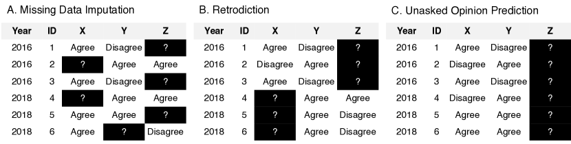
Figure 1: Three types of missing problems in survey research. Panels A-C illustrate three typical missing data challenges in survey research. Each row indicates an individual subject in a social survey across different periods, and each column (i.e., X, Y, and Z) indicates public opinion variables that we aim to measure. The machine learning task in each situation is to predict the unobserved values [?] in the black cells using the observed values in the white cells.

Fine-tuning Large Language Models with Nationally Representative Surveys

How can social scientists address these challenges of predicting unmeasured responses in survey data? In 2020, a massive collaborative effort involving 160 teams of social scientists attempted to predict year-level missing responses using various missing data imputation and relevant machine learning techniques, which is akin to the aforementioned “retrodiction” task. They find that none of the approaches could produce highly accurate predictions (Salganik et al., 2020). Existing missing data imputation techniques struggle to handle these challenges due to the limitations posed by data sparsity and insufficient relevant information (Sengupta et al., 2023). Traditional missing data imputation techniques and other relevant machine learning techniques (Sengupta et al., 2023; Salganik et al., 2020) presume that survey data encompasses all crucial variables required to predict missing responses for a specific variable. Yet, given the constraints on the number of questions that can be included in a survey, it is not always feasible to ask every question that are needed for imputing missing responses. For example, the GSS started to ask a question about respondents’ LGBT status after 2008, which could be highly predictive of support for same-sex marriage. It would be hard for the traditional imputation models without the information about LGBTQ status to accurately predict support for same-sex marriage. Even if all relevant variables were included in the survey data, existing methods might fail to predict entirely missing responses each year or completely new questions that have not been asked before.

Recent studies insist that LLMs could be a next-generation solution for addressing these issues (Argyle et al., 2023). Namely, the remarkable capabilities of LLMs in imitating what humans would generate in the next token sequence can be useful for opinion prediction (Argyle et al., 2023; Santurkar et al., 2023; Schramowski et al., 2022) because LLMs are trained by a wide array of text data, including data with Q&A (questions & answers) formats. For example, the model may be able to infer human-like responses to “Do you agree with legalizing same-sex marriage” by choosing the answer that is most likely to occur based on the training data. However, existing LLMs are known to have limitations in accurately and equally representing populations across various socio-demographic groups (Santurkar et al., 2023; Abid et al., 2021), accounting for individual heterogeneity (Argyle et al., 2023; Gordon et al., 2022; Kirk et al., 2023), and estimating past opinions due to their imbalanced training on recent text data (Longpre et al., 2023; González-Gallardo et al., 2023; Kozlowski et al., 2019). In a nutshell, we need to assume that the training data for LLMs is unbiased and representative of the general population, an assumption that has been challenged by previous research (Santurkar et al., 2023).

Here, we propose a new methodological framework by fine-tuning LLMs to predict individuals’ survey responses using the General Social Survey (GSS), a nationally representative survey of Americans’ opinions since 1972 (Davern et al., 2021; Marsden et al., 2020). Fine-tuning is the process of partially updating the parameters of LLMs using a relatively small set of data, enabling these models to perform specific tasks more accurately. Specifically in the context of survey data, fine-tuning enables the alignment of LLMs with an individual with specific beliefs or values, bypassing the need to train the model with a large amount of text information from scratch. Here, we exploit the overlooked fact that surveys collect data through a series of texts with the same Q&A format that can be used during fine-tuning processes. By incorporating texts of survey questions as part of training data in addition to patterns of unique individual survey responses, our fine-tuned LLMs enable personalized prediction of individual responses to various questions. Specifically, our models can capture the textual nuances of survey questions reflected in the training corpus and infer how individuals interpret the meaning of questions differently based on their response patterns. Consequently, our approach can address methodological challenges associated with previously non-imputable missing data and unasked opinions, as shown in Panels B and C of fig. 1, more effectively.

We present an overview of our approach to personalizing LLMs to predict public opinion in fig. 2. Our approach first predicts individuals’ opinions and then aggregates them at the population level using survey weights to account for sample selection bias (Panel A). Assuming accurate prediction of opinions across individuals and effective accounting for sample selection bias through survey weighting, the predictions generated by our method can be deemed representative of the population. However, the standard architecture of LLMs does not account for individual variability in responses, making it challenging to personalize predictions to suit specific individual beliefs and opinions that are distinct from others. Therefore, we need to customize the architecture of LLMs to be suitable for predicting personalized responses to survey questions over time. In doing so, we incorporate the three most important neural embeddings for predicting opinions – survey question semantic embedding, individual belief embedding, and temporal context embedding – that capture latent characteristics of survey questions, individual heterogeneities, and survey periods, respectively (Panel B). Similar to word embeddings that position similar words close together, these neural embeddings represent similarities in the meanings of survey questions, individual beliefs, and temporal contexts in high-dimensional vector spaces. Then, our models use these latent features to predict the most plausible answer to a specific question for each individual at a given moment. This novel architecture enables our models to recognize that survey responses to the same question can vary among individuals and across different time periods.

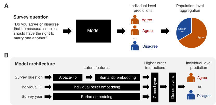
Figure 2: An overview of our methodological framework. In Panel A, we use survey weights when aggregating individual-level prediction into population-level estimates to account for potential sampling bias. In Panel B, individual belief and period embeddings are initially randomly assigned but optimized during the fine-tuning process using dense and cross layers. Semantic embedding, initially estimated by pre-trained LLMs (e.g., Alpaca-7b), is also optimized during the fine-tuning stage.

Initially, we use sentence-level embeddings from LLMs pre-trained on vast text corpora to encode the meaning of survey questions, such as “Do you agree or disagree that homosexual couples have the right to marry one another,” which are mapped into a latent vector space (Jurafsky and Martin, 2023). Table A1 demonstrates that the pre-trained LLMs accurately understand the semantic meaning of survey questions and generate human-like answers even before fine-tuning. We then fine-tune them using actual survey responses to better suit survey contexts. During this process, the embedding layers’ weights are updated to make an accurate prediction of a binary response to questions (0 or 1), resulting in questions with similar response patterns being closely located in the embedding space. Consequently, seemingly unrelated questions can be positioned more closely if it enhances prediction accuracy due to their similar response patterns (see Table A2). To determine the optimal model for generating the best predictions, we conduct extensive experiments with three LLMs with varying architectures and parameters (Alpaca-7b, GPT-J-6b, RoBERTa-large) (Liu et al., 2019; Taori, Rohan et al., 2023; Wang and Komatsuzaki, Aran, 2021).

A breakthrough we made for personalizing LLMs is to incorporate individual belief embeddings to account for individuals’ heterogeneous responses to survey questions based on heterogeneous belief systems (Baldassarri and Goldberg, 2014; Milbauer et al., 2021). To generate individual belief embeddings, we initially assign random latent features for each individual and optimize them during the fine-tuning process such that two individuals closely located in this embedding space have a similar set of beliefs (Gordon et al., 2022). Finally, we use period embeddings to consider temporal changes in the meaning of questions and individuals’ belief systems (Joo and Fletcher, 2020; Rule et al., 2015). To generate period embeddings, we initially assign random latent features for each period, which are optimized such that two adjacent periods characterized by similar response patterns are located close to each other in the latent space during the fine-tuning process. Figure A1 shows a two-dimensional projection of three embedding spaces. Finally, we consider the higher-order interactions between three embeddings by utilizing a deep learning architecture called “Deep Cross Network” (DCN) with a classification layer that predicts binary survey responses (Gordon et al., 2022; Wang et al., 2021). For detailed information, please refer to Appendix A.

Data and Method

Data

Our model framework allows us to predict how a given individual will respond in a given time period to an existing question for (A) missing data imputation, (B) retrodiction and (C) unasked opinion prediction, using their answers to other questions in a survey. We fine-tune pre-trained LLMs on the General Social Survey (GSS), a nationally representative survey in the United States. The GSS dataset provides comprehensive information about the demographic characteristics, political and ideological beliefs, cultural tastes, personal morality, and diverse attitudes of people in the United States. We use 68,846 individuals’ responses to 3,110 questions collected for 33 repeated cross-sectional data between 1972 and 2021 for fine-tuning the LLMs. The use of the publicly available GSS data does not constitute research with human subjects because there is no direct interaction with any individual, and no identifiable private information is used. We retrieve the text content of GSS survey questions from GSS data explorer.

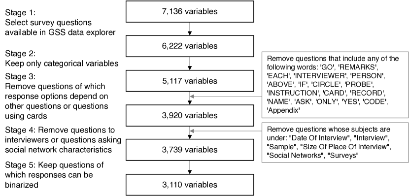
Figure A2: Variable selection process. Among all 7,136 variables in the initial GSS repeated cross-sectional data, we follow the five steps to finalize the list of 3,110 variables in our analytic sample. We download variable information from the GSS data explorer, the official general social survey website that provides the survey questionnaire (https://gssdataexplorer.norc.org/).

To provide more straightforward interpretations of the different response options, we transform them into a binary response by assigning a value of 1 to positive responses (e.g., agree, yes, true, likely) and 0 to negative responses (e.g., disagree, no, false, unlikely) through a combination of manual coding and machine-learning models (see Table A3 for top 50 response options). For instance, positive responses such as “strongly agree” and “agree” were coded as 1, while negative responses such as “strongly disagree” and “disagree” were coded as 0. To do so, we combine machine learning techniques and manual human coding. We find that our models demonstrate higher or comparable predictive accuracy for the binarized variables relative to the original binary variables (see the result section, individual-level and opinion-level heterogeneity of model accuracy). Among all 7,136 questions, we omit questions that rely on answers to other questions (for instance, if answering question B required selecting a specific response in question A), questions with a continuous response scale, and questions with an excessive number of response categories (see Figure A2 for the variable selection process), which finally leads to the final analytic sample of 3,110 questions of which responses could be binarized.

Fine-tuning Models

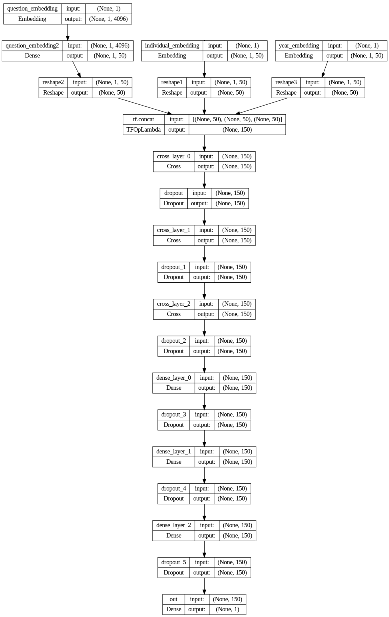
Figure A3: Model Architecture. Here, we present input and output dimensions for each layer: question_embedding = survey question semantic embedding, individual_embedding = individual belief embedding, year_embedding = period embedding, Cross= cross layers, Dense= feed-forward dense layers.

fig. 2 presents our end-to-end model architecture. Figure A3 provides additional information regarding the input and output dimensions of each layer. Our approach to personalizing LLMs is model-agnostic, meaning we can generate personalized responses using any LLM. For example, we can employ either decoder-only transformer models with billions of parameters (e.g., ChatGPT, GPT-4, Alpaca, GPT-J) or encoder-only transformer models (e.g., BERT, RoBERTa). Given the limited availability and reproducibility issues of private LLM models (e.g., ChatGPT and GPT-4) despite their impressive performance (Aiyappa et al., 2023), we opt for three widely-used open-source alternatives that demonstrate competitive performance in previous natural language processing benchmark tests: Alpaca-7b, GPT-J-6b, and RoBERTa-large (Liu et al., 2019; Taori, Rohan et al., 2023; Wang and Komatsuzaki, Aran, 2021).

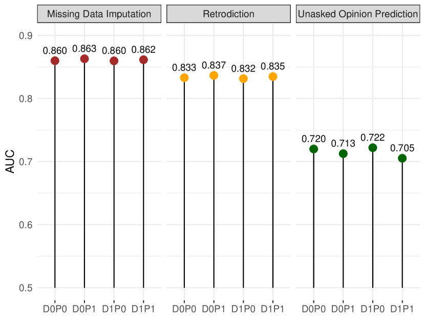
Figure A4: Model performance with or without demographics or partisanship information. We use the personalized LLMs based on Alpaca-7b to measure the AUC of models for missing data imputation, retrodiction, and unasked opinion prediction using one of the ten folds in the 10-fold cross-validation scheme. The notation D1P1 indicates that demographic information (i.e., age, cohort, gender, race, education, income, and religion) and partisanship information (i.e., political ideology, party affiliation) are used as training data. D1P0 indicates that demographic information is used, but partisanship information is not. D0P1 indicates that partisanship information is used, but demographic information is not. Finally, D0P0 indicates that neither demographic nor partisanship information is used in the model training.

Our models are designed to process three inputs – survey questions, individual IDs, and the survey year – and generate the predicted probability of each response option as an output. The models encode survey questions into a semantic embedding, while individual ID and survey year are respectively encoded into individual belief and period embeddings. These embeddings are then concatenated and used as inputs to the DCN, which then captures the higher-order interactions between them and generates the predictions. During the fine-tuning process, all embeddings and the DCN are jointly trained to generate predicted probabilities for response options. In doing so, we utilize Huggingface’s API for incorporating LLMs (Alpaca-7b, GPT-J-6b, RoBERTa-large) and TensorFlow Recommenders (TFRS) for deploying the DCN. During the fine-tuning process with the GSS data, model components are jointly trained with the DCN (see Appendix B for more details about model training). We find that using demographic features during the fine-tuning process does not significantly affect the models’ predictability, as shown in Figure A4. Based on these results, we exclude socio-demographic variables in the training data but include measures of a 7-point scale political ideology and party affiliation (i.e., Democrat, Republican, Independent, Others) that are known to be the important factors of opinion formation.

Our model architecture shares a similar design principle with other NLP models that aim to predict how different individuals label texts differently, such as the jury learning model  (Gordon et al., 2022). Simultaneously, our model architecture shares a similar goal with a group of models that use latent features to pinpoint key dimensions of beliefs underlying various opinions, such as principal component analysis (PCA) and the NOMINATE algorithm  (Joo and Fletcher, 2020). It is important to highlight that our model architecture does not impose any specific missing data mechanisms, such as Missing at Random (MAR) or Missing Completely at Random (MCAR). Instead, our model operates on the assumption that these latent factors influence responses, a concept similar to other machine learning models employed for deducing missing survey responses, like matrix factorization  (Sengupta et al., 2023). A key difference is that our models assume multiple latent features, including sentence embeddings, interact together to shape responses, while the matrix factorization model does not.

Model Evaluation

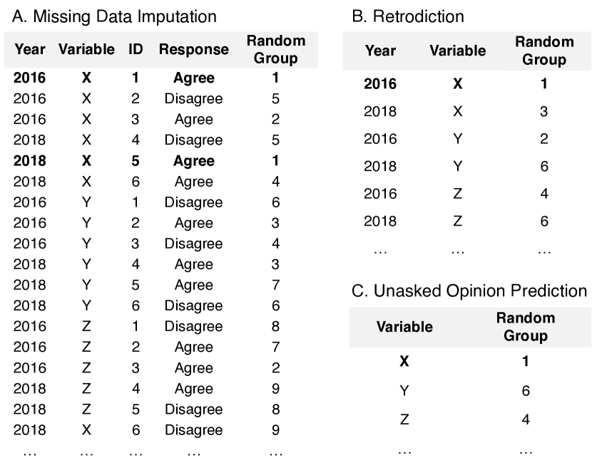
Figure A5: Examples of 10-fold cross-validation scheme. In Panel A, when predicting response-level missing opinions, we randomly allocate the combinations of year, variable, and individual ID into ten groups, which are held out in each round of cross-validation. In Panel B, when forecasting year-level missing opinions, we randomly assign pairs of year and variable into ten groups, which are held out in each round of cross-validation. In Panel C, when predicting completely missing opinions, we randomly assign variables into ten groups, which are held out in each round of cross-validation. Data in bold cells are excluded in the first round of cross-validation. By iterating these processes ten times, we can estimate the prediction we will get if responses are missing for the entire period, variables, and individuals.

We evaluate the model’s performance in predicting opinions at the individual and population levels in the GSS data by conducting 10-fold cross-validation to measure their accuracy in restoring missing data (see Figure A5). Specifically, for predicting response-level missing opinions in the missing data imputation task, we randomly remove 10% of responses and attempt to predict them using the model. For the year-level missing opinions in the retrodiction task, we randomly remove 10% of survey questions per survey year and predict the responses to them. For the entirely missing opinions in the unasked opinion prediction task, we randomly select 10% of survey questions and completely remove the responses to them for all survey years. For each task, we repeat this procedure ten times to guarantee accurate predictions for all questions, ensuring that the test data is not included in the training data.

Throughout the analysis, we will present AUC (Area Under the receiver operating characteristic Curve; i.e., the extent to which models accurately predict positive responses over their prediction of negative responses on a scale ranging from 0 to 1, where 1 represents the perfect prediction and 0.5 is equivalent to a random guess) because it does not require an arbitrary threshold to binarize the predicted values . We take the survey-weighted average of the predicted probability to measure the proportion of positive responses at the population level and measure correlations between observed responses and predicted responses across all available years to evaluate the validity of our public opinion prediction. Finally, we investigate the performance of our models against missing data arising from three different assumptions: Missing Completely at Random (MCAR), Missing at Random (MAR), and Missing Not at Random (MNAR) (see Appendix C and D for more details on the model evaluation and simulation of missing data).

As we formulate predicting opinions in a survey as imputing missing responses, we consider matrix factorization as a benchmark. Despite the extensive development of missing data imputation models using statistical relationships between variables, existing methods struggle to recover missing data when survey responses are sparse (Sengupta et al., 2023). Recent studies show that machine learning techniques, such as matrix factorization, can fill in missing responses better than traditional missing imputation models when the existing data are sparse (Blumenstock et al., 2015; Sengupta et al., 2023), making it the ideal benchmark for our tasks requiring the prediction of extremely sparse responses, such as “retrodiction”.Given that the matrix factorization models do not consider the textual information of survey questions using this as a benchmark allows us to examine how considering the meaning of survey wording and phrases and their interactions with latent factors improve the performance of opinion prediction (see Appendix E for more details on the matrix factorization model).

Results

Model Performance for Personal Opinion Prediction

Table A4 shows that Alpaca-7b provides the best results overall across all three tasks among the three LLMs and matrix factorization model. It confirms that LLMs with a larger number of parameters show better performance. Interestingly, while the predictive performance gaps across four models are small for missing data imputation, the gaps become larger for retrodiction as fewer human responses are used during the fine-tuning process, with the largest gaps observed for unasked opinion prediction.

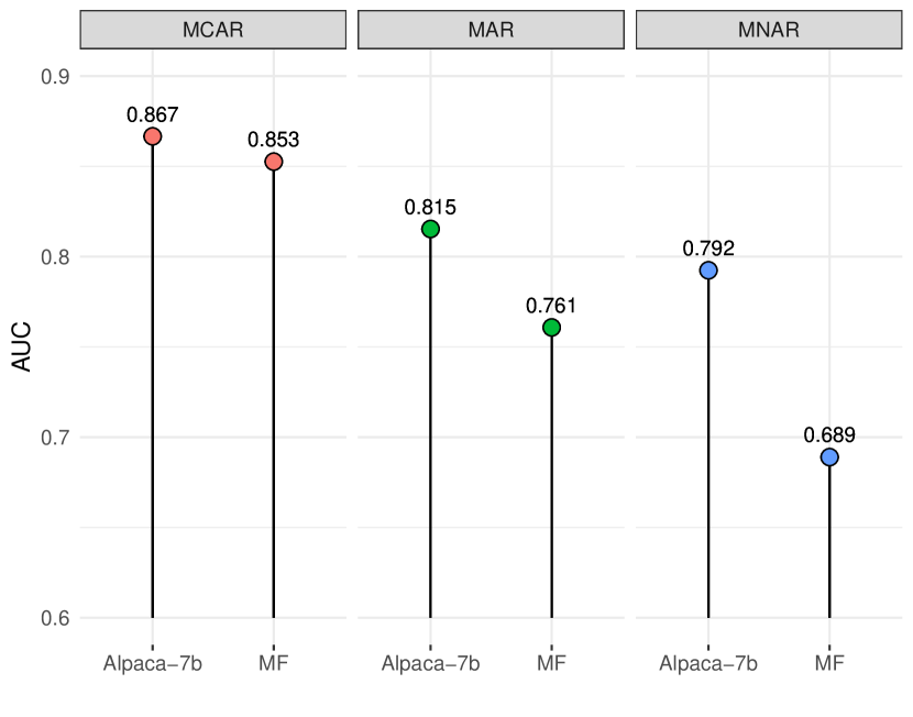
Figure A6: Performance of Alpaca-7b and matrix factorization models for missing data imputation by different missing mechanisms. AUC (Area Under Curve) measures the performance of the model in predicting data that are MCAR (missing completely at random), MAR (missing at random), and MNAR (missing not at random) as indicated by each bar. MF: Matrix factorization.

fig. 3, Panel A displays the performance of the best model (i.e., Alpaca-7b) for individual-level predictions across three tasks. Our top-performing model succeeds in the missing imputation task (AUC = 0.866), though the matrix factorization model also shows a similar level of performance (AUC = 0.852). Given that the matrix factorization model presumes that data are missing completely at random (MCAR) — a stronger assumption than the missing at random (MAR) principle that underlies standard multiple imputation frameworks — it is essential to examine how our models operate across various missing data mechanisms. Using the simulated GSS data based on three different mechanisms (MCAR, MAR, and MNAR: Missing Not At Random), Figure A6 shows that our model performs better under MCAR, MAR, and MNAR compared to matrix factorization. These findings indicate that our model performs better in inferring answers for not only randomly skipped responses, as seen in split-ballot designs, but also for non-random systematic refusal.

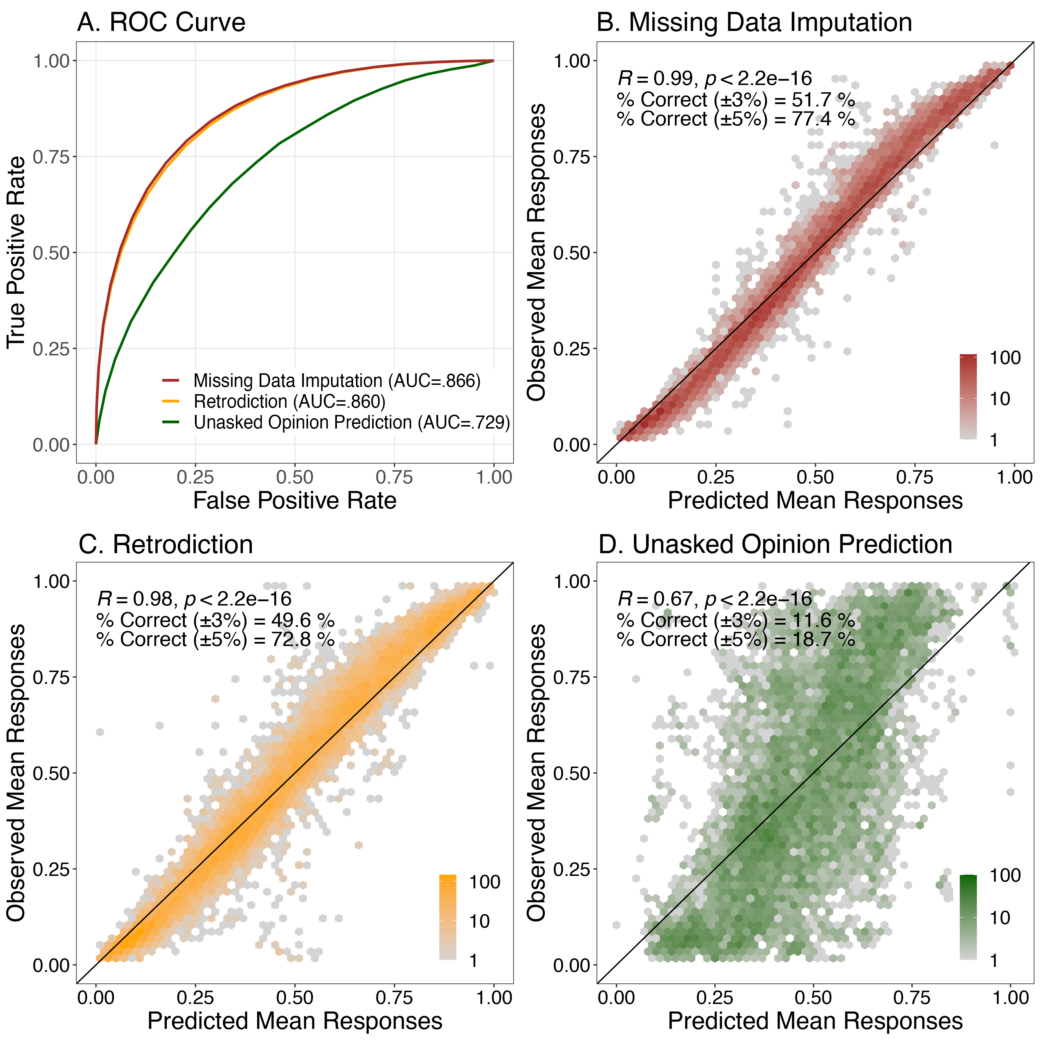
Figure 3: Model performance for predicting three types of missing responses at individual and aggregate levels. Panel A displays the Receiver Operating Characteristic (ROC) curve, indicating how well a model can predict missing responses at an individual level. We also denote the AUC (Area Under Curve) values, i.e., the probability of the model ranking a randomly selected positive response over a randomly selected negative response. Panels B-D depict the relationship between the observed proportion of those who agree in a survey each year and the predicted proportion of the agreement for the same opinion. The percentage of correct predictions within a margin of error of 3% is indicated as ”% Correct ± 3%,” which implies that the difference between the actual and predicted opinions is 3% or less. We color the predictions that fall within this range.

Our model also succeeds in the retrodiction task (AUC = 0.860), where it needs to predict the entirely missing responses in a certain year, significantly outperforming the matrix factorization model (AUC = 0.798). We further conduct a posthoc analysis to figure out how our model can generate highly accurate predictions based on sparse survey data by assessing the relative importance of features used in our model (Wang et al., 2021). Table A5 presents the importance of various features in our model based on Alpaca-7b. Specifically, we estimate F using the weights of the first cross layer from the DCN. We find that the semantic embedding capturing the meaning of survey questions makes the largest contribution to predictions (0.243), which is followed by the interactions between semantic and period embeddings (0.192). These results suggest that the higher performance of our models compared to the matrix factorization model may arise from the advanced capabilities of LLMs in processing the meaning of survey questions and from its consideration of complex interactions between period embeddings and two other embeddings that aid in contextualizing model predictions across different periods.

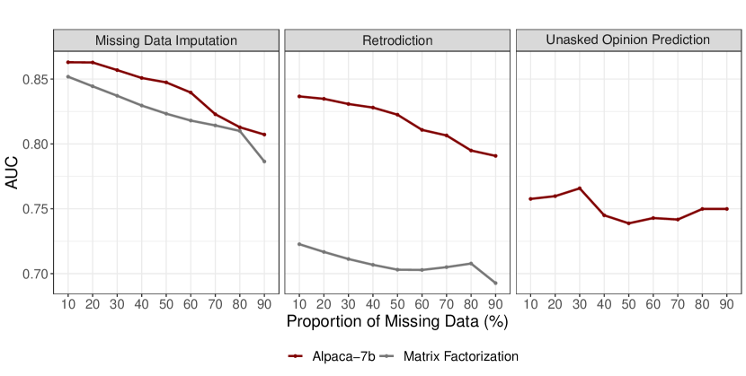
Figure A7: Model performance by the proportion of missing data in training data (10% to 90%). X-axis indicates the proportion of missing data in the training data. For instance, 10% indicates that only 10% of the existing data has been used to train the model. Y-axis indicates the AUC values for missing data imputation, retrodiction, and unasked opinion prediction which are estimated using one of the ten folds in the 10-fold cross-validation scheme.

The unasked opinion prediction task remains challenging even with LLMs with billions of parameters, such as Alpaca-7b (seven billion parameters, AUC=0.733) and GPT-J-6b (six billion parameters, AUC=0.693). Our model’s lower performance in the unasked opinion prediction task implies that it is harder to predict an individual’s opinion on a question that has never been asked in the survey than on a question that has been asked and answered by other individuals at least once in any other periods. However, bigger LLMs still outperform smaller models like RoBERTa-large (AUC = 0.571), which is consistent with the finding that upscaled LLMs significantly enhance task-agnostic, zero-shot, or few-shot performance without fine-tuning (Brown et al., 2020). To understand the nature of the large gap in AUCs between the retrodiction and unasked opinion prediction models (0.860 vs 0.733), we evaluate the predictive performance of models fine-tuned with varying amounts of missing data from 10% missing to 90% missing. Figure A7 shows that performances of missing data imputation and retrodiction models decrease as a smaller amount of training data is used during the fine-tuning process, though it is not always the case for unasked opinion prediction models. In sum, these results demonstrate that personalized LLMs better predict opinions when trained with more human survey responses.

Model Performance for Public Opinion Prediction

Predicting public opinion is a separate challenge from predicting personal opinion, as it requires accounting for varying probabilities of sample selection when we aggregate personal opinions. For instance, if the sampling weights for Black respondents are higher than those for White respondents, biases in our estimates—when weighted by sampling weights—will become greater when the predictive accuracy is lower among Black individuals. Yet, Panels B-D reveal that performances of public opinion prediction largely mirror individual-level results. Missing data imputation and retrodiction models that rely on existing human responses show very high correlations between the observed proportions of positive responses and the predicted proportions for opinions measured in each survey year ($\rho$ > 0.98), indicating that our predictions can be reliably used for trend estimation and correlational analysis. For predicting the population proportion, our models with the conventional 3% margin of error can predict approximately 50% or more of true survey responses in these two scenarios.

However, our model shows a relatively low correlation ($\rho$ = 0.68) in unasked opinion prediction. This result suggests that researchers should be very cautious when using LLMs to replace trend estimation and correlational analysis in social science research or high-stake decision-making. For predicting the population proportion, our model with the 3% margin of error can predict only about 12% of true survey responses in the unasked opinion prediction task. Even with the 5% margin of error, our model can predict only 18.7%, which is much lower than 77.4% and 72.8% from both missing data imputation and retrodiction models, respectively. The lower performance of unasked opinion prediction models for public opinion prediction highlights how difficult it is to make a precise prediction at the aggregate levels, even with a decent size of correlations and relatively high individual-level accuracy.

Retrodicting Counter-factual Trends

How can we utilize the near-perfect correlations between the predicted and observed responses from our retrodiction model? fig. 4, Panels A1-A4, present counter-factual trends of selected opinions from our models that retrodict what would likely be observed had these opinions been asked throughout the entire period. We selected them because they showcase the representative case scenarios in four typical applications of retrodiction based on the average AUCs and the patterns of observed years . We compare the retrodicted trends from the best model against those from the matrix factorization model (Panels B1-B4), which serves as a null model because it is a simpler model assuming that individuals’ attitudes on an opinion can be predicted by their attitudes on other opinions that best predict it when it is asked.

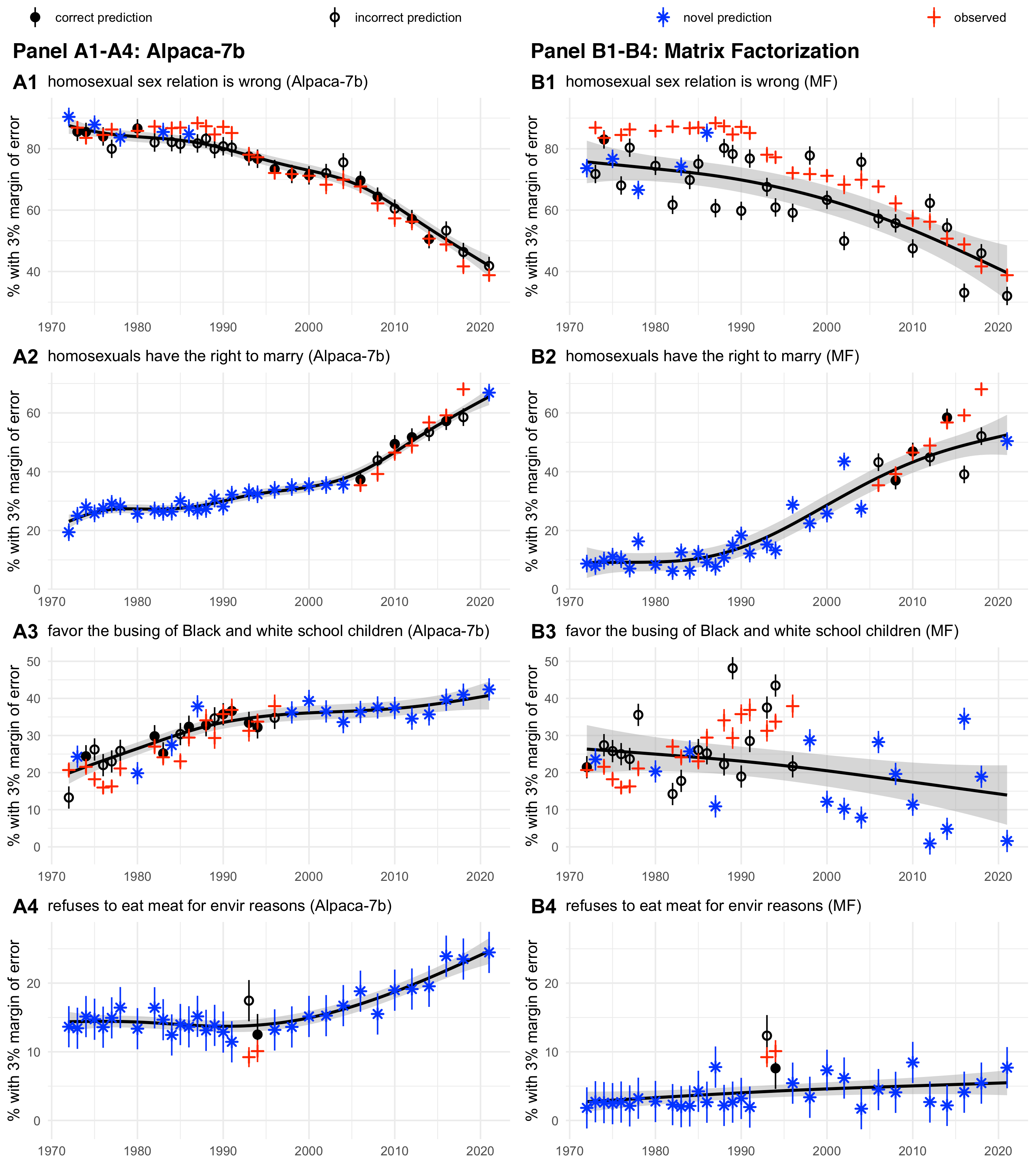
Figure 4: Illustration of the potential application of our models and matrix factorization models for predicting counter-factual trends in the GSS 1972-2021. The generalized additive model was used to estimate the counterfactual trends. We define the correct prediction when the prediction interval within 3% margin of error includes the observed estimate. The variable name, response option, and wording of questions for each panel are followed: Panels A1, B1. “What about sexual relations between two adults of the same sex–do you think it is always wrong (=1), almost always wrong(=1), wrong only sometimes (=1), or not wrong at all (=0)?” (homosex). Panels A2, B2. “Do you agree or disagree with the following statement? Homosexual couples have the right to marry one another. Strongly agree (=1), agree (=1), neither agree nor disagree (=0), disagree (=0), strongly disagree (=0)” (marhomo1). Panels A3, B3. “In general, do you favor or oppose the busing of (Negro/Black/African-American) and white school children from one school district to another? Favor (=1), Oppose (=0)” (busing). Panels A4, B4. “And how often do you refuse to eat meat for moral or environmental reasons? Always or Often (=1), Sometimes or Never (=0)” (nomeat).

There are several core questions that the GSS continues to ask for a long time to effectively track changes in public opinion and ensure their validity and reliability. One of them is about attitudes toward homosexual relationships. Our fine-tuned models, based on Alpaca-7b, can predict it within a 3% margin of error for most years (Panel A1), but predictions from matrix factorization models are mostly incorrect (Panel B1). Interestingly, both models can predict that fewer Americans think that homosexual relationships are wrong in more recent periods. Although the GSS survey has asked this question nearly every year, our predictions might still be useful for filling in missing responses in years when it was not asked.

As societal changes occur, the GSS likely modifies its questions to reflect them. The GSS board might have begun incorporating new questions when they recognize issues as being salient, such as gay rights in 2008, following events like Massachusetts’ legalization of same-sex marriage in 2004, or they might have discontinued old questions as issues’ prominence and relevance in social and political conversations diminished over time, for example, a decline in the use of busing as a racial desegregation tool in the 1990s. Panels A2 and A3 demonstrate how our model predictions can be useful for filling in missing responses to questions asked only during specific periods. Panel A2 displays the counterfactual trends for the proportion of Americans agreeing that homosexuals have the right to marry one another before 2008. While matrix factorization models can also predict the general upward trend of support for gay marriage (Panel B2), they make incorrect predictions for most periods and underestimate them in the 1970s and 1980s.

One unique aspect of this same-sex marriage question is that the GSS asked a slightly different version of the same question as part of ISSP’s Family and Gender module, which includes the word “should” in the sentence in 1988, 2004, and 2021. Figure A8 shows that both results are quite similar, but the question including the word “should” predicts a slightly lower rate of agreement. This result demonstrates the reliability of our predictions across different variables with similar meanings while capturing the nuanced role of question-wording differences. Panel A3 presents the counterfactual trends for the proportion of Americans who would favor desegregation busing policy (i.e., whether they support busing Black and white school children together from one school district to another) even after the GSS stopped asking this question. It suggests that public opinion on racial busing would have remained largely unchanged since 1996.

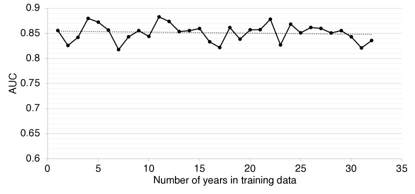
Figure A9: Number of years per survey question in training data and AUC in retrodiction. X-axis indicates the number of years per survey question in training data. For instance, the value of 1 indicates the case when a survey question is asked only once. Y-axis indicates the AUC values for year-level missing opinions.

Moreover, our models can retrodict counterfactual trends, even for questions asked only once or twice over five decades. For instance, the vegetarian population in the United States has been growing, but official statistics are scarce, with the GSS data only capturing this information in 1994 and 1996. Panel A4 illustrates the counterfactual trends of the proportion of Americans who consistently or frequently abstain from eating meat due to moral or environmental reasons. Although this opinion has been measured only twice, our model could estimate the trend we would observe if we had measured this opinion repeatedly over time. Our model predicts that roughly 25% of Americans always or often would refuse to eat meat for moral or environmental reasons in 2018, with the proportion steadily increasing since 1996 (Panel A4). In contrast, the trend estimations from the matrix factorization model do not seem to adequately capture the societal shifts toward a more progressive society (in Panels B3 and B4). At this point, one may wonder how we can trust counterfactual trends based on only a few years of observations. Figure A9 shows that the predictive performance of our models stays the same regardless of how many years each opinion is used as part of training data during the fine-tuning process.

Individual-level and Opinion-level Heterogeneity of Model Accuracy

Despite the impressive capability of our models in making a fairly accurate prediction of personal and public opinion, it is crucial to recognize that not all individuals and opinions are equally predictable. fig. 5 shows the performance of our Alpaca-7b based model across various subgroups, including sex, age, period, race, region, education, income, and political ideology, across three scenarios. We estimate OLS regression models to assess between-group gaps in individual-level AUCs with robust standard errors.

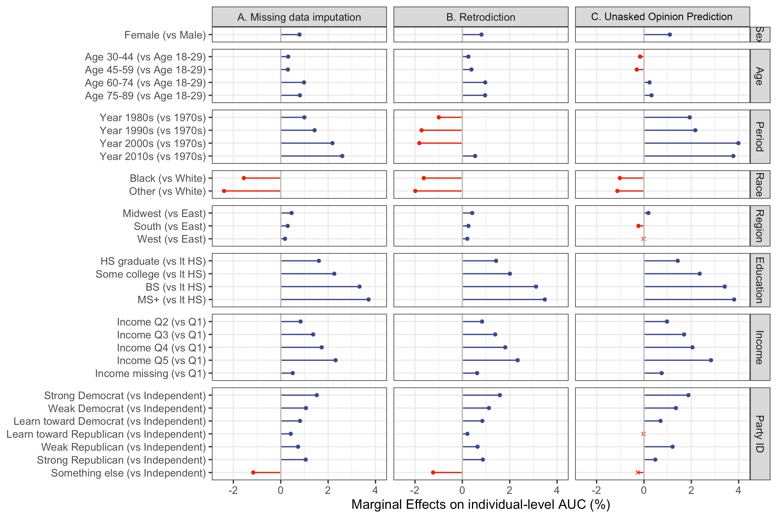
Figure 5: Coefficient plots from OLS regression models predicting individual-level AUC across three different types of missing response prediction. A higher AUC value indicates greater model accuracy for individuals. Here, each dot represents the expected difference of AUC (i.e., average marginal effects) against the reference group within each subgroup with the 95% confidence intervals. Red bars indicate that the AUC for a particular group is below the AUC of the reference group, and blue bars indicate that the AUC for a particular group is above the AUC of the reference group. Here, a filled dot refers to a statistically significant difference, and an X refers to a statistically insignificant difference based on robust standard errors (p < 0.05).

First, opinions of individuals with higher socioeconomic status (SES), as measured by their levels of education and income, are more predictable than those with lower SES. Namely, individuals with a master’s degree or higher are more predictable than those without a high school degree, as indicated by a 0.037 higher AUC, whereas those in the top 20% income bracket are more predictable than those in the bottom 20%, with a 0.023 higher AUC. Second, our model’s prediction is less accurate for racial minorities than Whites by a 0.015 lower AUC. Third, our models can predict strong partisans more accurately than Independents and “something else” groups. Lastly, we observe a higher AUC in more recent periods. This suggests that, despite our implementation of period embedding, our models still produce less accurate predictions for past opinions, with an AUC decrease of up to 0.025 for the 1970s.

fig. 6 shows which factors are associated with opinion-level AUCs. Our best models confirm the recency bias using a linear survey period indicator (i.e., higher accuracy in predicting opinions in more recent surveys). One might question whether our models exhibited a different performance in 2021 when the survey response rate was 17%, the lowest in the history of GSS (the average response rate in the GSS was 72%), and the survey mode was altered due to the COVID-19 pandemic. However, we find no significant evidence to support this conjecture. The larger sample size (i.e., the number of respondents who answer a specific survey question in the training data) is obviously associated with the larger AUC, but this sample size effect is negligible in unasked opinion prediction. Opinions with higher response rates show higher AUCs though they are not significant for unasked opinion prediction. Surveys that use split ballot designs show better performance, encouraging more active use of split ballot designs in surveys. One might question whether predicting opinions with multiple response options, given our binarization method, is harder than those with just two options. However, we find minor effects, only in the case of unasked opinion prediction models. The proportion of non-responses, such as refusals or inapplicable responses, is associated with the lower AUCs, highlighting the challenge of predicting opinions with fewer responses due to systematic non-responses.

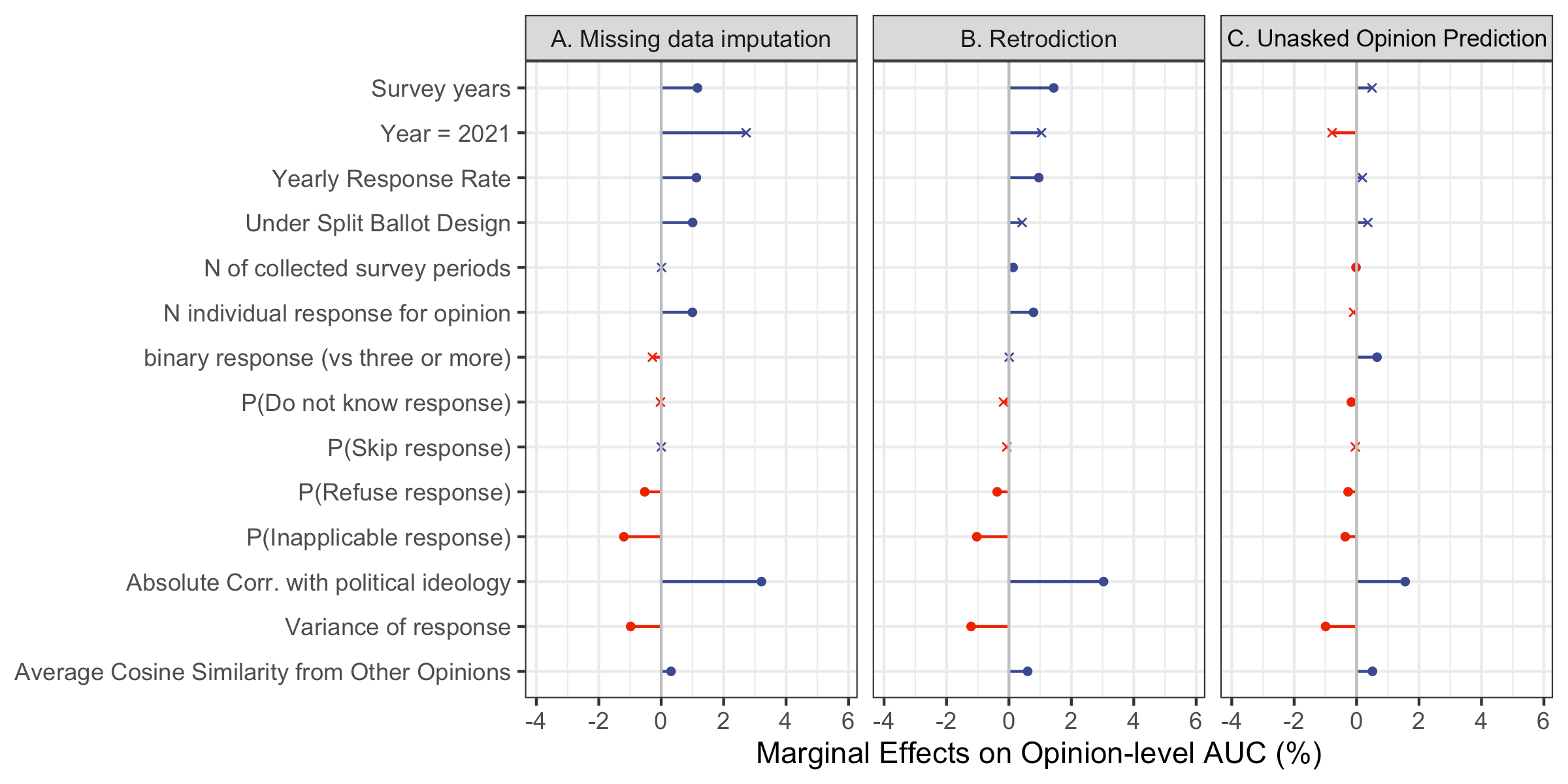
Figure 6: Coefficient plots from OLS regression models predicting opinion-level AUC across three different types of missing response prediction. A higher AUC value indicates greater model accuracy for opinions each year. Here, each dot represents the average marginal effects of each variable. To compare the effect size across different continuous covariates, we standardize them in regression analysis. Red bars indicate that the variable is negatively correlated with opinion-level AUC, and blue bars indicate that the variable is positively correlated with opinion-level AUC. Here, a filled dot refers to a statistically significant difference, and an X refers to a statistically insignificant difference based on robust standard errors (p < 0.05).

The strongest factor that affects opinion-level AUCs is the extent to which opinions are correlated with seven-scale political ideology. It should not be surprising given the strong evidence of ideological sorting in public opinion (Baldassarri and Gelman, 2008; Boutyline and Vaisey, 2017). For instance, the following opinions are highly correlated with a measure of political ideology with a correlation coefficient of 0.53: whether women with low incomes or unmarried women should have the right to undergo an abortion legally. Our models effectively retrodicted these opinions, achieving impressive AUCs of 0.94 and 0.95, respectively. In contrast, the association between individuals’ dissatisfaction with work situations and their political ideology was extremely weak, with a correlation coefficient of less than 0.01. The model’s accuracy in retrodicting this belief was also very low, yielding an AUC of 0.57. On the other hand, an AUC is smaller when the survey response shows a larger variance, indicating that it is harder to predict a controversial opinion. Additionally, the models can better predict opinions closely located with other opinions in the embedding space measured by the average cosine similarity with all other opinions, but its magnitude is less than 0.01. This means that the model is capable of accurately predicting opinions not only that are semantically similar, as illustrated in Table A2, but also that deviate from other opinions in the sentence embedding space.

Discussion

Artificial Intelligence (AI) agents have been with us for a long time, taking various forms such as recommender algorithms that learn and predict individual preferences and, more recently, conversational AIs that serve diverse needs (e.g., ChatGPT) (Rahwan et al., 2019). With the recent advancements in LLMs demonstrating remarkable performance in mirroring human behaviors and responses, the possibility of replacing human participants with AI agents in social science research has been suggested (Dillion et al., 2023; Bail, 2023). Some studies in biological sciences have already employed in-silico AIs to replace costly in-vivo experiments and advance scientific discovery (Jumper et al., 2021), and recent scholarship has started exploring this possibility in social sciences as well (Argyle et al., 2023; Chu et al., 2023; Dillion et al., 2023; Ziems et al., 2023). In fact, survey researchers rank highest among the professions whose tasks can be significantly impacted by LLMs (Eloundou et al., 2023). Now is the time to ask this question: Can LLMs replace social surveys?

Our answer is that LLMs are more useful in augmenting, rather than completely replacing, human responses in surveys. In social sciences, accurately predicting public opinion remains a challenge because it is a collective representation of diverse personal opinions and most individuals do not always hold consistent and coherent beliefs towards various issues (Baldassarri and Goldberg, 2014; Zaller and Feldman, 1992; Converse, P., 1964). While public opinion is generally stable over time with individuals holding firmly to their beliefs (Kiley and Vaisey, 2020), some attitudes (e.g., same-sex marriage) undergo dramatic shifts (Baunach, 2012). Against this background, recent studies employing LLMs show limited successes in predicting public opinion accurately and raise questions of demographic representativeness (Santurkar et al., 2023). It is presumably because the existing LLMs lack the capability to address individual heterogeneities and temporal dynamics. With a flexible methodological framework to tackle these challenges, we show that personalized LLMs are more suitable for certain survey-based applications with human inputs – missing data imputation and retrodiction. At the same time, personalized LLMs show limited capacity when human-generated responses are not readily available, such as unasked opinion prediction, challenging the idea of replacing human subjects with AI agents.

How can social scientists and decision-makers benefit from our AI-augmented survey methodology? We demonstrate that fine-tuning LLMs with nationally representative surveys enables us to effectively predict a wide range of public opinion while reducing the loss in accuracy or representativeness, tackling the challenges inherent in both digital trace and survey data. The practical applicability of our model for missing data imputation arises from its consistently high accuracy, irrespective of the extent of missing data and different missing mechanisms. Figure A7 demonstrates that more training data always performs better for missing data imputation and retrodiction. However, in the absolute sense, our missing data imputation models with 10% training data show a higher than 0.8 AUC. To elaborate on this finding, we examine how many questions are needed to develop models with reasonably high AUCs. Figure A10 shows that even only asking 10 questions achieved a good performance (AUC = 0.77), and the performance gain peaked at asking 100 questions (AUC = 0.83). This capability can be useful when survey designs are expected to be impacted by significant attrition in the current era of declining response rates (Sengupta et al., 2023). This approach can also be advantageous in designing opinion-tracking polls to maximize the number of questions posed to a given number of respondents. For instance, rather than asking the same ten questions to a thousand participants, pollsters can disseminate twenty questions among the same thousand participants, each answering ten questions, and employ the model to infer individual responses to the remaining ten unasked questions. On the other hand, given our model’s remarkable ability to mimic human responses, even including biases, researchers can use it to refine their survey questions by systematically examining characteristics of questions that cannot be accurately predicted (e.g., poor question wording).

Our model with high accuracy in the retrodiction tasks can help us identify a turning point by looking into past trends – when they started to shift. Some may question whether our models can predict unmeasured opinion trends, even during periods of exogenous shocks such as COVID-19. As demonstrated in Figure 6, there was no significant variation in the performance of our model when predicting unmeasured opinions in 2021 compared to other periods. We speculate that this high level of accuracy arises because the vanilla LLMs, such as Alpaca-7b, were pre-trained on rich digital traces during the COVID-19 period, and the period embedding captures temporal dynamics precisely. Our model’s ability to capture public opinion that has changed dramatically is supported by its accurate prediction of the sudden change in attitudes supporting same-sex marriage and opposition to eating meat. Furthermore, our models can aid survey designers in formulating survey questions. For example, they could leverage the model’s future predictions to prioritize questions that are anticipated to uncover unexpected trends.

Finally, despite its limited performance in unasked opinion prediction without any human response to entirely new questions compared to other tasks, our best model using Alpaca-7b still shows an AUC of 0.729 in predicting personal opinions. This performance is comparable to or higher than the performance of recent LLMs without fine-tuning in zero-shot prediction tasks in social science, such as sentiment analysis and ideology detection (Ziems et al., 2023). We may benefit from this capability to inspire scientific discovery, such as assisting in the selection of relevant survey questions and discovering meaningful hypotheses that involve currently unobserved data (Holm, 2019). For example, researchers may pre-register their analysis plans by generating advanced predictions, or they may even conduct a preliminary analysis of simulated data, based on which they can propose new research hypotheses and confirm them by conducting an actual survey with human participants. Moreover, the model can help pinpoint which demographic groups or individuals might benefit from oversampling to ensure improved survey quality and representation, given the relatively small accuracy gaps in unasked opinion prediction across different demographic groups shown in fig. 5. Despite its potential advantages, nonetheless, it is crucial to underscore this point: Under no circumstances should these predictions be employed directly for high-stake decisions that have tangible impacts on individuals. The ethical implications and potential for unintended consequences are too significant to ignore.

What can we learn from these results with regard to the nature of personal and public opinion? The remarkable performance of our predictive models suggests that the notion of personal opinion may not be as personal as it seems. The predictability of personal opinions highlights the inherently social nature of human beings, suggesting that our opinions are embedded in the social contexts that we belong to. This may not be surprising given that LLMs, trained on vast amounts of human-generated text, encode a wide spectrum of human attitudes, as humans utilize technological devices to voice their opinions into the socio-technical reservoir, which in turn, through algorithmic confounding, constrains and shapes what they perceive, observe, and generate (Latour, 2007). Some people might be surprised by the LLMs’ ability to extract relevant information from this extensive record of human history. Other people might not be surprised since it may reaffirm the old idea that most citizens’ question-and-answer process in a survey merely involves recalling a blend of partially consistent ideas, including an overrepresentation of ideas made salient by question prompts, much like the retrieval process of LLMs, which are then used to respond to the question (Zaller and Feldman, 1992).

The higher predictability of individuals with higher SES and stronger partisanship is largely aligned with a theory of political belief systems; namely, they tend to hold coherent belief systems in which opinions are highly correlated to each other (Zaller and Feldman, 1992; Converse, P., 1964). The lower predictability of racial minorities should remind us of the recent finding that the meaning of the terms “liberal” and “conservative” is unfamiliar to many black Americans (Jefferson, 2020). However, these patterns may also indicate potential biases in LLMs pre-trained based on a large text corpus (e.g., CommonCrawl) that arise from digital divides by SES (DiMaggio et al., 2004; Nadeem et al., 2020). To ascertain the origins of accuracy gaps across varying demographic groups, we compare the regression outcomes between LLMs and matrix factorization models. Given that matrix factorization models do not use any textual information, biases from matrix factorization models may indicate the extent of biases attributable to group differences in belief systems, as opposed to a biased pretraining corpus. Figure A11 displays similar patterns between the two models, suggesting that these gaps are likely a result of different levels of belief organization across different demographic groups.

Our study brings several ethical concerns into focus concerning the use of LLMs to predict personal and public opinion. A major concern lies in the realm of privacy and surveillance. Our models have demonstrated the ability to accurately estimate personal opinions that respondents might not be willing to share or may have chosen not to answer. The implications of this could be far-reaching, especially when such tools could be misused by organizations, for example, to screen job applicants based on information that individuals have not explicitly agreed to disclose. This risk escalates as the models grow more precise in predicting opinions and as more people trust and use these models. Therefore, it is crucial to engage in discussions about how we can maintain respondent privacy and data protection while concurrently enhancing the accountability and responsibility of generative AIs (Shevlane et al., 2023). The urgency of initiating conversations to prevent potential misuse cannot be overstated.

Parallel to concerns of privacy and surveillance, ethical considerations regarding individual autonomy and demographic representation are of equal importance. Despite its accuracy, predicting a person’s opinion without their consent can be seen as a potential infringement on their autonomy. This is especially apparent when an answer is presumed on their behalf when they either refuse to respond or express uncertainty. This concern widens when viewed from a societal perspective, particularly in contexts of democracy since autonomous opinion formation is a fundamental component of democratic processes (Burstein, 2003; Shapiro, 2011). Surveys are traditionally seen by participants as platforms to voice their opinions and influence democratic outcomes (Igo, 2008). The potential shift from surveys filled out by individuals to those generated by AI could significantly disrupt the formation of democratic consensus. Our model’s lower accuracy for individuals with low socioeconomic status, racial minorities, and non-partisan affiliations can exacerbate the demographic representation issue. For instance, if decision-makers use these kinds of models to guide policy implementation, the less predictable voices of minority groups could be marginalized. This could further undermine the already fragile trust in surveys.

There are some limitations to the proposed AI-augmented survey approach worth noting. First, our current models dichotomize response options into positive and negative ones for the sake of an intuitive understanding of opinions. However, researchers often use a five-point scale ranging from “strongly disagree” to “strongly agree” to gauge the extent of agreement or disagreement. Future studies might improve this issue by incorporating multi-class classification layers or decoders, enabling them to predict opinions with more than two response options. Second, our internal cross-validation procedure yields high levels of accuracy and strong correlations between observed and predicted responses, which enhance our confidence in retrodicting counterfactual trends. However, some may cast doubt on the external validity of our model’s ability to retrodict. To address this potential limitation, future research could employ cross-survey validation. This would involve examining whether the models, fine-tuned via the General Social Survey, can accurately predict missing opinions in other nationally representative surveys (e.g., the American National Election Survey) and vice versa.

Third, a more thorough set of benchmark tests is needed to probe the potential of this methodology when applied to local and online surveys that lack national representativeness. For example, researchers can ask the same set of questions utilized by the GSS concurrently in their own survey and use the fine-tuned model based on the GSS data to predict responses to other questions that were not asked. At present, it is uncertain how useful our approach can be for predicting opinions in non-representative surveys conducted only once or twice with a small number of respondents. Finally, most LLMs are pre-trained on recent text data, which may lead to contextual discrepancies, considering that the meaning of words can shift across different historical contexts (Longpre et al., 2023; González-Gallardo et al., 2023; Kozlowski et al., 2019). Take the word “artificial” as an example; it was previously used to denote something skillfully designed, akin to “artistic.” Now, it is primarily used to indicate something that is not natural such as artificial flavors and artificial intelligence. Although we have tried to address this issue by integrating interactions between period and sentence embeddings in our models, we find that predictability in the 1970s is still lower than in the 2010s.

Against this background, we anticipate that these limitations may soon be addressed as the scale of LLMs expands and more scholarly focus is directed toward enhancing the integration of LLMs with social surveys for opinion prediction. We believe that our research marks a foundational step and has shown promising potential for the future of social science research using the LLMs. With the rapid advancement in LLM-related applications, more and more survey researchers may consider using the AI-augmented survey approach or similar kinds. Upon the publication of our article, we will make our code and data available in an accessible way through Github, packages, and other channels to facilitate the replication and extension of our novel approach. In the meantime, we encourage interested researchers to refer to the model training and evaluation codes in Appendix F to use our methodology.

Appendix for AI-Augmented Surveys: Leveraging Large Language Models and Surveys for Opinion Prediction

Appendix A. Introduction to model architecture

Here, we introduce our model architecture designed to address major challenges arising from data sparsity issues when predicting personal and public opinion in more detail. First, traditional missing imputation techniques, including the advanced machine-learning models such as matrix factorization, fall short in predicting responses for new questions beyond the training data, as they are unable to extrapolate the meaning of survey questions (e.g., Panel C in Figure 1) (Sengupta et al., 2023). Our proposed model architecture addresses this challenge by encoding survey questions into sentence embeddings using pre-trained large language models. A large language model (LLM) refers to a type of neural network that possesses an extensive number of parameters, typically in the billions or more, trained on vast amounts of unlabeled text data using self-supervised learning (Vaswani et al., 2017). These pre-trained models encode the meaning of sentences into neural embeddings, which can be utilized for generating subsequent tokens or identifying subsequent sentences (e.g., responses to questions).

Specifically, to encode survey questions to neural embeddings, we pass survey questions into the LLMs and extract the last token’s embedding for decoder-only models (Alpaca and GPT-J) and a special token embedding (or pooler output) for encoder-only models (RoBERTa-large). We employ the following prompt, based on Alpaca's instruction data template (Taori, Rohan et al., 2023), to extract semantic embeddings from pre-trained LLMs: “Below is an instruction that describes a task. Write a response that appropriately completes the request. ### Instruction: [SURVEY QUESTION] ### Response: ” To ensure that the semantic embedding accurately captures the meaning of survey questions, we have the model generate text-based responses using this embedding and assess whether the responses align with what humans might say. In most cases, the models generated human-like answers, indicating that the embedding contains rich semantic information about the survey question (see Table A1). LLMs have different dimensions of embeddings. For instance, Alpaca-7b has 4096 dimensions, while RoBERTa-large has 1024 dimensions. We use a single feed-forward layer to convert the original embedding to an identical N-dimensional trainable semantic embedding, regardless of the model's original dimensionality (See Figure A3). During the fine-tuning process, semantic embeddings are fine-tuned based on the response patterns in the survey. Specifically, sentence embeddings are contextualized such that two questions with similar response patterns are more closely mapped within the embedding space. This enables the fine-tuned models to learn the common socio-cultural meaning of survey questions and predict appropriate responses. As a result, the fine-tuned models learn to interpret the meaning of new questions, such as “Do you agree with a law requiring police permission to purchase a gun?” and locate them in the semantic embeddings based on the expected patterns in survey responses in the way the predictability of responses is maximized. Table A2 presents survey questions that are most similar to four questions used in Figure 4 in the embedding space, which allows us to see how the model captures the similarity in meanings of questions as well as their response patterns in surveys. We refer to this embedding vector, $s\ \in\ R^{n}$  as the “semantic embedding” of survey questions.

Second, recent approaches like in-context tuning utilize various prompts to adapt LLMs to represent specific group opinions (Brown et al., 2020), but they fail to account for unique individual perspectives because these methods can only predict the commonly held opinions of a “typical” group (Argyle et al., 2023; Santurkar et al., 2023). To address these challenges, we add an additional layer of neural embedding in our model architecture – individual belief embedding. Traditional machine learning models have primarily focused on producing a single output for a given input. For instance, when given an input sentence like “the weather is so good,” models for sentiment analysis are designed to generate a single output, such as “it conveys a positive sentiment.” However, this method may not generate reliable responses for controversial issues. For example, when asked about their stance on gun control in the United States, people’s responses will likely be influenced by their pre-existing beliefs. Recent studies have developed a methodological framework that accounts for individual heterogeneity, recognizing that people possess diverse opinions (Gordon et al., 2022; Park et al., 2021). Building on the insights from these models that assign labels on an individual basis, instead of applying a uniform label to everyone, we assume that each individual’s beliefs are represented as an N-dimensional embedding vector. We refer to this vector, $b\ \in\ R^{n}$, as the “belief embedding” of individuals.

Third, existing approaches overlook temporal heterogeneities in the interpretation of survey questions and individual belief systems. To address this, we incorporate period embedding as the third layer of neural embeddings. This accounts for the impact of temporal factors on survey question responses, such as the gradual shift towards more progressive beliefs over time (Baldassarri and Park, 2020) and the effects of specific events during a particular period, like macroeconomic changes, presidential elections, and the COVID-19 pandemic. While some argue that people’s beliefs are generally stable, attributing fluctuations in opinions to short-term changes or measurement errors (Kiley and Vaisey, 2020; Ansolabehere et al., 2008), others contend that social transformations and life events can indeed lead to lasting shifts in perspectives (Lersch, 2023). We represent the historical features of survey periods as an N-dimensional embedding vector, which we refer to as the “period embedding” of surveys, denoted by $p\ \in\ R^{n}$.

Finally, we incorporate the higher-order interactions between the three embeddings related to survey question meanings, individual beliefs, and historical contexts by employing a new deep learning architecture called the “Deep Cross-Network (DCN)” (Gordon et al., 2022; Wang et al., 2021). The DCN comprises multiple cross layers designed to capture feature interactions and feed-forward dense layers, or classifier head, that are responsible for generating the final prediction. By employing a sigmoid function, the final prediction is generated as a predicted probability, which falls within the range of 0 to 1. This value represents the likelihood that an individual will indicate a positive response (e.g., agree, yes) to a particular survey question.

In the following example, we demonstrate how the DCN operates. Let’s assume that $s_{1}$ captures whether a question is about vaccine hesitancy, $b_{1}$ captures whether an individual holds conservative ideology, and $p_{1}$ captures the extent to which the COVID-19 pandemic is ongoing. If an individual’s response to a vaccine mandate is influenced by their conservative ideology and the ongoing COVID-19 pandemic, we will need to consider the interaction $s_{1}\times b_{1}\times p_{1}$ to predict the individual’s response. To capture these interactions, we define cross layers in the DCN as follows. We begin by concatenating the semantic embedding of the survey question ($s$), the individual’s belief embedding ($b$), and the temporal embedding ($p$) into a single vector, denoted as $x_{0}$. The (l+1)th cross layer can then be defined as follows:

$$x_{l+1}=x_{0}\ \odot\ (W_{l}x_{l}+b_{l})+x_{l}$$

where $x_{l}\ \in\ R^{3n}$ and $x_{l+1}\ \in\ R^{3n}$ are the input and output of the cross layers, respectively. $W_{l}\ \in\ R^{3n\times 3n}$ and $b_{l}\ \in\ R^{3n}$ are the learned weights and biases of the cross-layer. Each element in $W_{l}$ captures the relative contribution of the interaction between features in the prediction. In the DCN with k cross layers, the model includes all feature interactions up to a maximum polynomial order of k + 1.

By concatenating multiple cross layers, it is possible to consider more complex interactions. For instance, the relationship between attitudes toward vaccine mandate and being a liberal might depend on another latent dimension, such as one’s attitudes toward scientific knowledge. Complex feature crossings like $s_{1}\times b_{1}\times b_{2}\times p_{1}$ can be captured by employing multiple cross layers. By considering complex interactions between the meaning of survey questions, individual beliefs, and survey periods, we can avoid the assumption that the meaning of opinions is identical for everyone over time. This assumption has been challenged by previous research on the heterogeneous perception of cultural meanings across different socio-demographic backgrounds (Goldberg, 2011; Baldassarri and Goldberg, 2014) and cognitive biases (Martin, 2010).

Figure 2 presents our end-to-end model architecture. Figure A3 provides additional information regarding the input and output dimensions of each layer. We first encode survey questions into a semantic embedding using Alpaca-7b, GPT-J-6b, or RoBERTa-large, while individual ID and survey year are respectively encoded into individual belief and period embeddings. These embeddings are then concatenated and used as inputs to the DCN, which then captures the higher-order interactions between them and generates the predictions. During the fine-tuning process, all embeddings and the DCN are jointly trained to generate predicted probabilities.

Appendix B. Model training

To implement our model architecture, we utilize Huggingface’s API for incorporating LLMs (Alpaca-7b, GPT-J-6b, RoBERTa-large) and TensorFlow Recommenders (TFRS) for deploying the DCN. During the fine-tuning process with the GSS data, all model components are jointly trained with the DCN. We freeze the pre-trained parameters of LLMs, except for an adaptable, feed-forward layer to convert the original contextual embedding to an N-dimensional trainable semantic embedding, to avoid the known overfitting issues when jointly trained with other embeddings (Gordon et al., 2022), such as individual belief and period embeddings, which helps in keeping computational costs at a manageable level. From our experiments with RoBERTa-large, we learn that models without freezing the parameters did not meaningfully improve the performance. We fine-tune our models using the Adam optimizer with a learning rate of 2e-5, and a binary cross-entropy is used as the loss function. We use a batch size of 128, and we limit the maximum sequence length to 150 tokens for the RoBERTa-large model. For the DCN-specific architecture, we experiment with various hyperparameters and choose a fixed embedding dimension of 50, three cross-layers of size 150, three feed-forward dense layers of size 150, and a final output layer of size 1 based on the previous literature and a grid search (Gordon et al., 2022). The number of training epochs is determined based on the performance in validation data.

Appendix C. Model evaluation

Model evaluation: Personal opinion prediction

With the fine-tuned model, we can predict the probability that a respondent will positively respond to a specific survey question in a given year, which ranges from 0 (= negative response) to 1 (= positive response). We evaluate the model’s performance in “missing data imputation” (Figure 1, Panel A) through the following steps. We assess the model’s capability to predict missing opinions using 10-fold cross-validation. In practice, we randomly eliminate 10% of the responses from the training dataset and employ the model to predict these omitted responses (see also Figure A5, Panel A). For the response-level missing opinion (Panel A, Figure 1), we randomly distribute the combinations of survey years, survey questions, and individual IDs into ten groups. During the N-th iteration of cross-validation, the N-th group is excluded from the training data. The model is then trained on the remaining data for each round, and the excluded responses are predicted. By repeating this process ten times, we can infer the model’s predictive performance for all responses.

To assess the model’s ability in “retrodiction”, that is, predicting year-level missing opinions (Figure 1, Panel B), we employ a modified 10-fold cross-validation technique. In this case, we evaluate the model’s predictive accuracy when the entire set of responses to 10% of questions is omitted in a particular year. This scenario differs from the first one, where questions are “asked” but not answered by participants. By contrast, here we evaluate situations where questions are “not even asked” during a specific period. To accomplish this, we randomly remove around 10% of survey questions in a survey year from the training dataset and train the model to predict the removed responses (see Figure A5, Panel B). Specifically, we randomly assign pairs of survey years and questions into ten groups, which are withheld in each round of cross-validation. During each round, the model predicts the entire set of responses to these survey questions in the excluded survey years. We repeat this process ten times.

To assess the model’s ability for “unasked opinion prediction,” which refers to the prediction of entirely missing opinions (Figure 1, Panel C), we adopt a distinct 10-fold cross-validation method. In this scenario, we gauge the model’s predictive accuracy when 10% of existing survey questions have never been asked by survey designers during the entire survey period. To achieve this, we randomly eliminate around 10% of survey questions entirely from the training data and use the model to predict them (see Figure A5, Panel C). Specifically, we randomly allocate survey questions into ten groups, which are withheld during each cross-validation round. During each round, the model predicts the entire set of responses to these survey questions. By repeating this process ten times, we can infer the model’s predictive performance when the entire response is missing.

Once we obtain predicted probabilities for each of the three tasks, we assess the Area Under Curve (AUC) to evaluate the extent to which our models can separate positive responses from negative responses in their prediction. The AUC measures the probability of the model to rank a randomly selected positive response over a randomly selected negative response, which ranges from 0.5 (= random prediction) and 1 (= perfect prediction). We also assess two other metrics – accuracy and F-1 score – and find similar results, but we do not present them in the main manuscript because they require an arbitrary threshold for binarizing continuous predicted probabilities, which could be particularly problematic when the distribution of responses is imbalanced. In Table A4, reporting the AUC, accuracy, and F1 scores across different models and tasks, we use the threshold of 0.5 for accuracy and F1 scores.

Model evaluation: Public opinion prediction

We estimate public opinion by aggregating the predicted personal opinion while using survey weights. Specifically, the fine-tuned model predicts the probability that a particular individual will give a positive response to a particular survey question in a particular survey year. Then, we estimate the marginal proportion of individuals giving positive responses to the question by taking the weighted mean of predicted probabilities using survey weights to account for sample selection biases. In doing so, we use a linear regression model to rescale the predicted responses to be close to the observed responses when aggregated, which helps to minimize the error caused by the difference between the variation in predictions and observations. To evaluate the accuracy of public opinion predictions, we conduct 10-fold cross-validation to produce predicted probabilities and estimate correlation coefficients between the predicted and observed proportion of positive responses. High correlations indicate the linear association between the predicted and observed proportions, which enhances our confidence in using predicted opinions to capture public opinion trends, including unobserved opinions. Along with correlation coefficients, we use a conventional margin of error (3%) to evaluate how many of our predictions can estimate the observed mean for each survey. Specifically, we measure the percent prediction error by calculating the proportion of opinions that can be estimated by predicted agreement rates within a 3% margin of error. Finally, we predict counterfactual trends in Figure 4 using aggregated responses from retrodiction models. To estimate the direction and magnitude of over-time trends, we employ a Generalized Additive Model (GAM), a flexible, non-parametric regression technique capable of modeling complex, non-linear relationships between variables (Hastie, 1992).

Appendix D. MCAR, MAR, and MNAR simulation

Previous research on imputing missing data has explored three different assumptions about how missing data occurs: Missing Completely at Random (MCAR), Missing at Random (MAR), and Missing Not at Random (MNAR) (Sengupta et al., 2023). Since our evaluation process only assumes MCAR, we simulate the missing data based on the other two assumptions, MAR and MNAR, and re-evaluate the models to examine whether our models show similarly high accuracy. MCAR supposes that the cause of missing values in a variable is not related to the observed or unobserved values of any variable. MAR assumes that the reason for missing values relies only on the values of other observed variables and is not related to the values of the missing variable. MNAR assumes that the reason for missing values is dependent on the values of both observed and unobserved variables.

We simulate missing data created under these three assumptions and evaluate whether the model can anticipate the missing values for these three mechanisms. Let us assume that we have a dataset $X$ represented by a $n\times p$ matrix, where $i=1,\ldots,n$ denotes individuals and $j=1,\ldots,p$ denotes observed and unobserved variables. The elements of $X$ are denoted by $x_{i,j}$ which indicate the survey responses. Additionally, we define a matrix $M$ that indicates the locations of the missing values as a $n\times p$ matrix, where $m_{i,j}=1$ if $x_{i,j}$ is missing, and $m_{i,j}=0$ if $x_{i,j}$ is observed. $X_{\text{observed}}$ and $X_{\text{unobserved}}$ represent the observed and unobserved data in $X$, respectively. $\xi$ is a missingness parameter, which is random and independent of the data $X$.

First, MCAR assumes that $M$ is completely unrelated to the data $X$ – unrelated to both $X_{\text{observed}}$ and $X_{\text{unobserved}}$. In other words, $p(M=1|X,\xi)=p(M=1|\xi)$. To simulate missing data based on MCAR, we randomly selected 10% of observed values and removed them. Second, MAR assumes that $M$ depends on the observed values of other variables but not on unobserved variables that the missing data imputation model cannot consider. Therefore, $p(M=1|X,\xi)=p(M=1|X_{\text{observed}},\xi)$. To simulate missing data based on MAR, we adopt the method proposed by Sengupta and colleagues (2023) that fits a logistic regression model predicting $m_{i,j}$ using the values of other observed variables. Specifically, we used the observed variables that rarely have missing values (less than 10%) to predict $m_{i,j}$. Then, we remove the 10% of values with the highest probability of being missing based on the regression. Third, MNAR assumes that $M$ depends on both observed and unobserved data. Thus, $p(M=1|X,\xi)=p(M=1|X_{\text{observed}},X_{\text{unobserved}},\xi)$. To simulate missing data based on MNAR, we fit a logistic regression model that predicts $m_{i,j}$ using demographic variables (i.e., age, cohort, gender, race, education, income, and religion). Since demographic variables have not been used by the missing data imputation model in our main results, we assume that these variables are unobserved and use these variables to generate MNAR missing values.

Appendix E. Matrix factorization

To establish a benchmark model for comparison, we train a matrix factorization model, which is a well-established technique for solving matrix completion problems by estimating missing values based on available elements. This involves decomposing a matrix with known elements into two lower-dimensional matrices. By optimizing the dot products of these matrices to align with the known elements of the original matrix, accurate predictions for the missing values can be obtained. It achieves high accuracy comparable to deep learning models, making it a popular choice in recommender system development (Koren et al., 2009). Matrix factorization also outperforms traditional imputation methods, such as Amelia and MICE, in filling missing data in sparse survey datasets (Sengupta et al., 2023).

First, we create a matrix $S\ \in\ R^{68,846\times 3,110}$ of survey responses. Each row represents an individual, each column represents a survey question, and each element indicates the individual’s binarized response (0 = negative and 1 = positive, see Table A1). Using this matrix $S$, we train two lower-dimensional matrices: $I\ \in\ R^{68,846\times 50}$ and $Q\ \in\ R^{50\times 3,110}$. The objective is to optimize $I$ and $Q$ such that the dot product of the corresponding rows and columns closely matches the available values in $S$. Specifically, we minimize the squared difference $(I_{i\cdot}Q_{\cdot q}-S_{iq})^{2}$ for the available values in $S$. To optimize $I$ and $Q$, we employ the alternating least squares (ALS) method, following the previous study on the GSS 2014 data (Sengupta et al., 2023). We conduct ALS for 15 iterations, applying a regularization penalty of $\lambda=10$ to prevent overfitting. Using the learned latent factors from the matrix factorization model optimized throughout this process, we predict the missing response of an individual $i$ for a given variable $q$ by taking the dot product of the corresponding vectors: $I_{i\cdot}$ and $Q_{\cdot q}$.

Appendix F. Source code

The source code provided below outlines the implementation of our model’s architecture and details the processes of training and evaluating the model. The code assumes that the survey data has been preprocessed and converted into a dataframe format with five columns (gss.parquet): year, yearid, variable, question, and binarized. Each row in this dataframe represents an individual’s response to a specific question during a particular survey year (refer to Figure A5 for more details). Here, year denotes the survey year, yearid refers to the unique ID assigned to each survey participant, variable signifies the variable name in the GSS dataset, question describes the text of the survey question, and binarized indicates the binarized survey response (with 1 representing a positive response, and 0 a negative response). Given this setup, the subsequent steps in the code let you fine-tune the model and evaluate its performance.

⬇

1import pandas as pd

2from sklearn.preprocessing import LabelEncoder

3import time

4import pickle

5import random

6import os

7import numpy as np

8import pandas as pd

9from tqdm.auto import tqdm

10import torch

11import tensorflow as tf

12import tensorflow_recommenders as tfrs

13from tensorflow.keras import Model

14from tensorflow.keras.callbacks import ModelCheckpoint

15from tensorflow.keras.layers import Input, Dense, Dropout, Embedding, Reshape

16from transformers import AutoTokenizer, AutoModel, LlamaTokenizer, LlamaForCausalLM

17from sklearn.model_selection import train_test_split

18from sklearn.metrics import roc_auc_score, accuracy_score, f1_score

19

20# Setting random seed for reproducibility.

21os.environ[’PYTHONHASHSEED’] = str(42)

22random.seed(42)

23np.random.seed(42)

24torch.manual_seed(42)

25tqdm.pandas()

26

27df = pd.read_parquet(’gss.parquet’)

28

29# Generate ordered IDs for use in models (e.g., convert 20060001, 20060002, ... to 0, 1, 2)

30le = LabelEncoder()

31df[’yearid_id’] = le.fit_transform(df[’yearid’])

32df[’question_id’] = le.fit_transform(df[’variable’])

33df[’year’] = df[’yearid’] // 10000

34df[’year_order’] = le.fit_transform(df[’year’])

35

36# Load the Alpaca 7b model. Replace "Alpaca-7b" with the actual model name from Hugging Face, such as "Alpaca-7b", "GPT-J-6b", or "RoBERTa-base". Refer to this link to get the Alpaca-7b model: https://github.com/tatsu-lab/stanford_alpaca

37model_name = "Alpaca-7b"

38tokenizer = LlamaTokenizer.from_pretrained("Alpaca-7b")

39model = LlamaForCausalLM.from_pretrained("Alpaca-7b")

40

41# Iterate over survey questions, generate an Alpaca prompt template for each, and retrieve the embeddings of the last token.

42question_list = df[[’question_id’, ’question’]].drop_duplicates().sort_values(’question_id’)[’question’].tolist()

43embeddings = []

44for question in tqdm(question_list):

45 prompt = "Below is an instruction that describes a task. Write a response that appropriately completes the request.\n\n"

46 prompt += f"### Instruction:{question}\n\n### Response:"

47 input_ids = torch.tensor(tokenizer.encode(prompt)).unsqueeze(0)

48 outputs = model(input_ids, output_hidden_states=True)

49 embeddings.append(outputs.hidden_states[-1][:, -1, :].detach().numpy()) #last token embedding

50

51if ’/’ in model_name:

52 model_name = model_name.replace(’/’, ’_’)

53

54pickle.dump(embeddings, open(model_name+’.pkl’, ’wb’))

55

56train_data, val_data = train_test_split(df, test_size=0.1)

57train_data.to_parquet(’train_data.parquet’)

58val_data.to_parquet(’val_data.parquet’)

59

60# Split the dataset into training and validation sets. This example demonstrates the data splitting process specifically for a missing data imputation task.

61train_data, val_data = train_test_split(df, test_size=0.1)

62train_data.to_parquet(’train_data.parquet’)

63val_data.to_parquet(’val_data.parquet’)

64

65def get_model(dim=50):

66 # End-to-end model architecture

67 # Embedding 1: Individual Belief Embedding

68 weights = np.vstack(pickle.load(open(’chavinlo_alpaca-native.pkl’, ’rb’))) # Load the last token embeddings.

69

70 individual_id = Input(name=’individual_id’, shape=(1, ))

71 x1 = Embedding(df[’yearid_id’].max() + 1, dim, name=’individual_embedding’)(individual_id)

72 x1 = Reshape((dim, ), name=’reshape1’)(x1)

73 # Embedding 2: Survey Question Semantic Embedding (based on Alpaca)

74 question_id = Input(name=’question_id’, shape=(1, ))

75 question_embedding = Embedding(weights.shape[0], weights.shape[1], weights=[weights], name=’question_embedding’)(question_id)

76 question_embedding.trainable = False

77 x2 = Dense(50, name=f’question_embedding2’)(question_embedding)

78 x2 = Reshape((50, ), name=’reshape2’)(x2)

79 # Embedding 3: Period Embedding

80 year_id = Input(name=’year_id’, shape=(1, ))

81 x3 = Embedding(df[’year_order’].max() + 1, dim, name=’year_embedding’)(year_id)

82 x3 = Reshape((dim, ), name=’reshape3’)(x3)

83 # Concatenating three embeddings

84 x = [x1, x2, x3]

85 x = tf.concat(x, axis=1, name=’concat1’)

86 # Passing through cross layers

87 for i in range(3):

88 x = tfrs.layers.dcn.Cross(projection_dim=dim*3, kernel_initializer="glorot_uniform", name=f’cross_layer_{i}’)(x)

89 x = Dropout(0.2)(x)

90 # Passing through feed-forward layers

91 for i in range(3):

92 x = Dense(dim*3, activation="relu", name=f’dense_layer_{i}’)(x)

93 x = Dropout(0.2)(x)

94 # Generating final predictions

95 out = Dense(1, activation=’sigmoid’, name="out")(x)

96 inputs = {’individual_id’: individual_id,

97 ’question_id’: question_id,

98 ’year_id’: year_id}

99 model = Model(inputs=inputs, outputs=out)

100 return model

101

102def train(train, val):

103 model = get_model()

104 train_features = {’individual_id’: np.array(train[’yearid_id’]),

105 ’question_id’: np.array(train[’question_id’]),

106 ’year_id’: np.array(train[’year_order’])}

107 train_label = np.array(train[’binarized’])

108 val_features = {’individual_id’: np.array(val[’yearid_id’]),

109 ’question_id’: np.array(val[’question_id’]),

110 ’year_id’: np.array(val[’year_order’])}

111 val_label = np.array(val[’binarized’])

112

113 # Compiling the model

114 lr_schedule = tf.keras.optimizers.schedules.ExponentialDecay(

115 2e-05,

116 decay_steps=80000,

117 decay_rate=0.96,

118 staircase=True)

119 model.compile(

120 optimizer=tf.keras.optimizers.Adam(learning_rate=lr_schedule),

121 loss=tf.keras.losses.BinaryCrossentropy(),

122 metrics=[tf.keras.metrics.AUC(),

123 tf.keras.metrics.BinaryAccuracy()]

124 )

125 # Fitting the model to the data

126 history = model.fit(train_features, train_label,

127 validation_data=(val_features, val_label),

128 batch_size=8,

129 epochs=10,

130 verbose=1,

131 use_multiprocessing=True,

132 workers=20)

133

134 return model

135

136# Training the model

137train_data = pd.read_parquet(’train_data.parquet’)

138val_data = pd.read_parquet(’val_data.parquet’)

139trained_model = train(train_data, val_data)

140trained_model.save_weights(’missing_imputation.h5’)

141

142# Evaluate the model

143prediction_model = get_model()

144prediction_model.load_weights(’missing_imputation.h5’)

145obs = val_data[’binarized’]

146pred = prediction_model.predict()

147print(roc_auc_score(obs, pred), accuracy_score(obs, pred>0.5), f1_score(obs, pred>0.5))

Appendix Tables and Figures

Table A1: Examples of text responses generated by the Alpaca-7b model.

Variables	Survey questions	Text responses
homosex	What about sexual relations between two adults of the same sex–do you think it is always wrong, almost always wrong, wrong only sometimes, or not wrong at all?	I believe that sexual relations between two adults of the same sex is not wrong at all.
marhomo1	Do you agree or disagree with the following statement? Homosexual couples have the right to marry one another.	I agree.
busing	A. In general, do you favor or oppose the busing of (Negro/Black/African-American) and white school children from one school district to another?	I oppose the busing of (Negro/Black/African-American) and white school children from one school district to another.
nomeat	C. And how often do you refuse to eat meat for moral or environmental reasons?	I rarely refuse to eat meat for moral or environmental reasons.

Note: These responses were generated without reflecting a particular individual’s opinions in our training data. These responses were generated solely for checking whether the model understands the semantic meaning of survey questions correctly.

Table A2: Most similar survey questions.

Survey questions		Most similar survey questions		Cosine similarity
(homosex) What about sexual relations between two adults of the same sex–do you think it is always wrong, almost always wrong, wrong only sometimes, or not wrong at all?		(homosex1) C. And what about sexual relations between two adults of the same sex, is it. . .		0.949
		(teensex) There’s been a lot of discussion about the way morals and attitudes about sex are changing in this country. If a man and woman have sex relations before marriage, do you think it is always wrong, almost always wrong, wrong only sometimes, or not wrong at all? A. What if they are in their early teens, say 14 to 16 years old? In that case, do you think sex relations before marriage are always wrong, almost always wrong, wrong only sometimes, or not wrong at all?		0.781
		(premars1) A. Do you think it is wrong or not wrong if a man and a woman have sexual relations before marriage?		0.773
(marhomo1) Do you agree or disagree with the following statement? Homosexual couples have the right to marry one another.		(marhomo) Do you agree or disagree? J. Homosexual couples should have the right to marry one another.		0.951
		(grassy) Some people think the use of marijuana should be made legal. Other people think marijuana use should not be made legal. Which do you favor?		0.892
		(ssmchild) To what extent do you agree or disagree with the following statements? B. A same sex male couple can bring up a child as well as a male-female couple.		0.871

Table A2: Most similar survey questions (continued).

Survey questions		Most similar survey questions		Cosine similarity
(busing) A. In general, do you favor or oppose the busing of (Negro/Black/African-American) and white school children from one school district to another?		(busing10) B. Now, thinking about ten years ago, that is in 1972, did you then favor or oppose the busing of (Negro/Black) and white school children from one school district to another?		0.883
		(unvote) If an election were held with secret ballots, would you vote for or against having a union represent you?		0.810
		(defund) Favor or oppose reducing funding for police and instead funding social services		0.798
(nomeat) C. And how often do you refuse to eat meat for moral or environmental reasons?		(racpromo) Do you think your race or ethnic background makes your promotion opportunities better or worse?		0.860
		(sparts) Listed below are various areas of government spending. Please indicate whether you would like to see more or less government spending in each area. Remember that if you say ”much more,” it might require a tax increase to pay for it. H. Culture and the arts.		0.839
		(hapifwrk) Do you agree or disagree … D. A woman and her family will all be happier if she goes out to work.		0.836

Note: For each survey question in Figure 4, we present the most similar survey questions in the semantic embedding space. The variable names are presented in parenthesis. The similarity between two survey questions is measured by the cosine similarity between the two semantic embeddings of the two survey questions.

Table A3: Binary Transformation of Survey Response Options: Top 50 responses.

Rank		Response Options		N		Binarized
1		yes, no		1010		1, 0
2		strongly agree, agree, neither agree nor disagree, disagree, strongly disagree		210		1, 1, 0, 0, 0
3		strongly agree, agree, disagree, strongly disagree		115		1, 1, 0, 0
4		mentioned, not mentioned		60		1, 0
5		very likely, somewhat likely, not very likely, not at all likely		46		1, 1, 0, 0
6		too little, about right, too much		45		0, 0, 1
7		true, false		31		1, 0
8		strongly agree, agree, not agree/disagree, disagree, strongly disagree		31		1, 1, 0, 0, 0
9		agree, disagree		30		1, 0
10		strongly agree, agree, neither, disagree, strongly disagree		29		1, 1, 0, 0, 0
11		often, sometimes, rarely, never		28		1, 1, 0, 0
12		agree strongly, agree, neither agree nor disagree, disagree, disagree strongly		27		1, 1, 0, 0, 0
13		not at all, 1 or 2 times, 3-5 times, 6 or more times		26		0, 0, 1, 1
14		1 most desirable, 3 most desirable, not mentioned, 3 least desirable, 1 least desirable		26		1, 1, 0, 0, 0
15		strongly favor, favor, neither favor nor oppose, oppose, strongly oppose		23		1, 1, 0, 0, 0
16		never, 1-2 times, 3-5 times, more than 5 times		21		0, 0, 1, 1
17		strongly agree, agree, disagree, or, strongly disagree?		20		1, 1, 0, 0
18		definitely allowed, probably allowed, prob not allowed, definitely not allowed		20		1, 1, 0, 0
19		very likely, somewhat likely, somewhat unlikely, very unlikely		18		1, 1, 0, 0
20		very true, somewhat true, not too true, not at all true		18		1, 1, 0, 0
21		definitely should, probably should, probably should not, definitely should not		18		1, 1, 0, 0
22		like very much, like it, mixed feelings, dislike it, dislike very much		18		1, 1, 0, 0, 0
23		spend much more, spend more, spend same, spend less, spend much less		18		1, 1, 0, 0, 0
24		very important, important, somewhat important, not at all important		17		1, 1, 0, 0
25		very likely, somewhat likely, mixed, somewhat unlikely, very unlikely		17		1, 1, 0, 0, 0
26		essential, very important, fairly important, not very important, not important at all		17		1, 1, 1, 0, 0
27		did, didn’t		16		1, 0
28		strongly agree, somewhat agree, somewhat disagree, strongly disagree		16		1, 1, 0, 0
29		definitely willing, probably willing, probably unwilling, definitely unwilling		16		1, 1, 0, 0
30		should, should not		15		1, 0
31		strongly agree, agree somewhat, disagree somewhat, strongly disagree		15		1, 1, 0, 0
32		definitely expect, probably expect, probably not expect, definitely not expect		15		1, 1, 0, 0
33		a great deal of influence, a fair amount, a little influence, none at all		15		1, 1, 0, 0
34		strongly agree, agree, uncertain, disagree, strongly disagree		15		1, 1, 0, 0, 0
35		a reason, not a reason		14		1, 0
36		major reason, minor reason, not a reason		14		1, 0, 0
37		no, yes, respondent, yes, someone respondent knows, yes, both respondent and someone respondent knows		14		0, 1, 1, 1
38		1 not at all effective, 2, 3, 4, 5 extremely effective		14		0, 0, 0, 1, 1
39		remove, not remove		13		1, 0
40		a great deal, only some, hardly any		13		1, 0, 0
41		most important, 2nd most imp., 3rd most imp., not chosen		13		1, 1, 0, 0
42		very likely, somewhat likely, not too likely, not likely at all		13		1, 1, 0, 0
43		definitely true, probably true, probably not true, definitely not true		13		1, 1, 0, 0
44		allowed, not allowed		12		1, 0
45		no, yes		12		0, 1
46		too much, about the right amount, too little		12		1, 0, 0
47		extremely likely, somewhat likely, not too likely, not likely at all		12		1, 1, 0, 0
48		extremely dangerous, very dangerous, somewhat dangerous, not very dangerous, not dangerous		12		1, 1, 1, 0, 0
49		excellent, very good, good, fair, poor		12		1, 1, 1, 0, 0
50		many times a day, every day, most days, some days, once in a while, never or almost never		12		1, 1, 1, 0, 0, 0

Table A4: Comparison of prediction performances across four different models across three scenarios.

		Models
		Alpaca-7b	GPT-J-6b	RoBERTa-large	Matrix Factorization
Missing data imputation	AUC	0.866	0.864	0.859	0.852
	Accuracy	0.782	0.779	0.774	0.784
	F1-score	0.765	0.765	0.758	0.770
Retrodiction	AUC	0.860	0.859	0.853	0.798
	Accuracy	0.775	0.774	0.768	0.740
	F1-score	0.755	0.759	0.750	0.687
Unasked opinion prediction	AUC	0.729	0.687	0.566
	Accuracy	0.667	0.632	0.546
	F1-score	0.640	0.609	0.422

Note: The best-performing models are highlighted in bold. AUC (Area Under the receiver operating characteristic Curve) measures the probability of the model to rank a randomly selected positive response over a randomly selected negative response. Accuracy is calculated by (true positives + true negatives) / (true positives + false positives + true negatives + false negatives), and F1-score is calculated by 2 * (precision * recall) / (precision + recall). Matrix factorization methods cannot be applied for unasked opinion prediction.

Table A5: Feature Importance.

Types of embeddings	Feature importance
Semantic embeddings	0.243
Individual belief embeddings	0.112
Period embeddings	0.114
Interactions between semantic and individual belief embeddings	0.180
Interactions between semantic and period embeddings	0.192
Interactions between individual belief and period embeddings	0.128

Note: Higher feature importance score measures the relative contribution of specific features to the overall predictions. Let n be the dimension of each embedding, x $\in\ R^{150}$ be the concatenation of semantic, individual belief, and period embeddings, and $W\ \in\ R^{150\times 150}$ is the learned weights of the cross-layer based on x. The feature importance is estimated using the Frobenius norm. Specifically, the feature importance of semantic, individual belief, and period embeddings is given by $\sqrt{\sum_{i=1}^{50}\sum_{j=1}^{50}{{|W}_{ij}|}^{2}}$, $\sqrt{\sum_{i=51}^{100}\sum_{j=51}^{100}{{|W}_{ij}|}^{2}}$, $\sqrt{\sum_{i=101}^{150}\sum_{j=101}^{150}{{|W}_{ij}|}^{2}}$, respectively. The feature importance of the interactions between semantic and individual belief embeddings, interactions between semantic and period embeddings, and interactions between belief and period embeddings are given by $(\sqrt{\sum_{i=1}^{50}\sum_{j=51}^{100}{{|W}_{ij}|}^{2}}+\sqrt{\sum_{i=51}^{100}\sum_{j=1}^{50}{{|W}_{ij}|}^{2})}/2$, $(\sqrt{\sum_{i=1}^{50}\sum_{j=101}^{150}{{|W}_{ij}|}^{2}}+\sqrt{\sum_{i=101}^{150}\sum_{j=1}^{50}{{|W}_{ij}|}^{2})}/2$, $(\sqrt{\sum_{i=51}^{100}\sum_{j=101}^{150}{{|W}_{ij}|}^{2}}+\sqrt{\sum_{i=101}^{150}\sum_{j=51}^{100}{{|W}_{ij}|}^{2})}/2$, respectively. To normalize the feature importance values, they have been divided by the sum of all feature importance values.

Figure A1: The visualization of semantic embedding, individual belief embedding, and period embedding. In Panel A, a two-dimensional t-distributed stochastic neighbor embedding (t-SNE) projection of semantic embeddings among survey questions that belong to one of the top 10 most frequent categories (tags) in the General Social Survey (N=1458, 46.9% of the entire 3,110 questions) are presented, with points colored by clusters found by hierarchical clustering. The majority of survey questions under the categories of Children, Federal Government, Job, Religion, Political, Science, United States, and Work are clustered in the green area, while Computers and Internet questions are clustered in the orange area, Health questions are clustered in the pink area, and the remaining questions are clustered in the blue area. In Panel B, the t-SNE projection of 68,846 individuals is presented, with points colored by clusters found by hierarchical clustering. In Panel C, the t-SNE projection of 33-period embeddings (1972-2021) is presented, with points colored by survey years ranging from earlier periods to more recent periods.

Figure A8: Predicting counter-factual trends in the GSS 1972-2021 for two questions on support for same-sex marriage. The generalized additive model was used to estimate the counterfactual trends. We define the correct prediction when the prediction interval within a 3% margin of error includes the observed estimate. The variable name, response option, and wording of questions for each panel are as followed: Panel A. “Do you agree or disagree with the following statement? Homosexual couples have the right to marry one another. Strongly agree (=1), agree (=1), neither agree nor disagree (=0), disagree (=0), strongly disagree (=0)”. Panel B. “Do you agree or disagree with the following statement? Homosexual couples should have the right to marry one another. Strongly agree (=1), agree (=1), neither agree nor disagree (=0), disagree (=0), strongly disagree (=0)”.

Figure A10: Model performance by the number of survey questions in the training data. AUC (Area Under Curve) measures the probability of the model to rank a randomly selected positive response over a randomly selected negative response. The Y-axis of the graph represents the AUC score, which is an indicator of how well the model can accurately fill in response-level missing opinion data. The X-axis displays the number of survey questions in the training data. We only use survey participants in 2016, 2018, and 2021 for this analysis.

Figure A11: Comparison of results from OLS regression models predicting individual-level AUC across two different types of missing data imputation between Alpaca and matrix factorization models. A higher AUC value indicates greater model accuracy for individuals. Here, each dot represents the expected difference of AUC (i.e., average marginal effects) against the reference group within each subgroup. Here, a filled dot refers to a statistically significant difference, and an X refers to a statistically insignificant difference based on robust standard errors (p < 0.05).

References

- Abid et al. (2021) Abid, Abubakar, Maheen Farooqi, and James Zou. 2021. “Persistent Anti-Muslim Bias in Large Language Models.” In Proceedings of the 2021 AAAI/ACM Conference on AI, Ethics, and Society, pp. 298–306. Association for Computing Machinery.
- Aher et al. (2023) Aher, Gati, Rosa I. Arriaga, and Adam Tauman Kalai. 2023. “Using Large Language Models to Simulate Multiple Humans and Replicate Human Subject Studies. arXiv:2208.10264 [cs.CL].”
- Aiyappa et al. (2023) Aiyappa, Rachith, Jisun An, Haewoon Kwak, and Yong-Yeol Ahn. 2023. “Can We Trust the Evaluation on ChatGPT? arXiv:2303.12767 [cs.CL].”
- Ansolabehere et al. (2008) Ansolabehere, Stephen, Jonathan Rodden, and James M. Snyder. 2008. “The Strength of Issues: Using Multiple Measures to Gauge Preference Stability, Ideological Constraint, and Issue Voting.” The American Political Science Review 102:215–232.
- Argyle et al. (2023) Argyle, Lisa P., Ethan C. Busby, Nancy Fulda, Joshua R. Gubler, Christopher Rytting, and David Wingate. 2023. “Out of One, Many: Using Language Models to Simulate Human Samples.” Political Analysis https://doi.org/10.1017/pan.2023.2.
- Bail (2023) Bail, Christopher A. 2023. “Can Generative AI Improve Social Science? SocArXiv.” https://doi.org/10.31235/osf.io/rwtzs.
- Baldassarri and Gelman (2008) Baldassarri, Delia and Andrew Gelman. 2008. “Partisans without Constraint: Political Polarization and Trends in American Public Opinion.” American Journal of Sociology 114:408–446.
- Baldassarri and Goldberg (2014) Baldassarri, Delia and Amir Goldberg. 2014. “Neither Ideologues nor Agnostics: Alternative Voters’ Belief System in an Age of Partisan Politics.” American Journal of Sociology 120:45–95.
- Baldassarri and Park (2020) Baldassarri, Delia and Barum Park. 2020. “Was There a Culture War? Partisan Polarization and Secular Trends in US Public Opinion.” The Journal of Politics 82:809–827.
- Baunach (2012) Baunach, Dawn Michelle. 2012. “Changing Same-Sex Marriage Attitudes in America from 1988 Through 2010.” Public Opinion Quarterly 76:364–378.
- Beauchamp (2017) Beauchamp, Nicholas. 2017. “Predicting and Interpolating State-Level Polls Using Twitter Textual Data.” American Journal of Political Science 61:490–503.
- Behr and Iyengar (1985) Behr, Roy L. and Shanto Iyengar. 1985. “Television News, Real-World Cues, and Changes in the Public Agenda.” Public Opinion Quarterly 49:38.
- Berinsky (2017) Berinsky, Adam J. 2017. “Measuring Public Opinion with Surveys.” Annual Review of Political Science 20:309–329.
- Blumenstock et al. (2015) Blumenstock, Joshua, Gabriel Cadamuro, and Robert On. 2015. “Predicting Poverty and Wealth from Mobile Phone Metadata.” Science 350:1073–1076.
- Boutyline and Vaisey (2017) Boutyline, Andrei and Stephen Vaisey. 2017. “Belief Network Analysis: A Relational Approach to Understanding the Structure of Attitudes.” American journal of sociology 122:1371–1447.
- Brand et al. (2023) Brand, James, Ayelet Israeli, and Donald Ngwe. 2023. “Using gpt for market research.” Available at SSRN 4395751 .
- Brayne (2020) Brayne, Sarah. 2020. Predict and Surveil: Data, Discretion, and the Future of Policing. Oxford University Press.
- Brooks and Manza (2006) Brooks, Clem and Jeff Manza. 2006. “Social Policy Responsiveness in Developed Democracies.” American Sociological Review 71:474–494.
- Brown et al. (2020) Brown, Tom, Benjamin Mann, Nick Ryder, Melanie Subbiah, Jared D Kaplan, Prafulla Dhariwal, Arvind Neelakantan, Pranav Shyam, Girish Sastry, and Amanda Askell. 2020. “Language Models Are Few-Shot Learners.” Advances in neural information processing systems 33:1877–1901.
- Burstein (2003) Burstein, Paul. 2003. “The Impact of Public Opinion on Public Policy: A Review and an Agenda.” Political Research Quarterly 56:29–40.
- Cesare et al. (2018) Cesare, Nina, Hedwig Lee, Tyler McCormick, Emma Spiro, and Emilio Zagheni. 2018. “Promises and Pitfalls of Using Digital Traces for Demographic Research.” Demography 55:1979–1999.
- Chu et al. (2023) Chu, Eric, Jacob Andreas, Stephen Ansolabehere, and Deb Roy. 2023. “Language Models Trained on Media Diets Can Predict Public Opinion. arXiv:2303.16779 [cs.CL].”
- Converse, P. (1964) Converse, P. 1964. “The Nature of Belief Systems in Mass Publics.” In Ideology and Discontent, edited by Apter, D. E., pp. 206–261. The Free Press.
- Couper (2017) Couper, Mick P. 2017. “New Developments in Survey Data Collection.” Annual Review of Sociology 43:121–145.
- Davern et al. (2021) Davern, Michael, Rene Bautista, Jeremy Freese, Stephen L. Morgan, and Tom W. Smith. 2021. “General Social Surveys, 1972-2021 Cross-section [machine-readable data file, 68,846 cases]. Principal Investigator, Michael Davern; Co-Principal Investigators, Rene Bautista, Jeremy Freese, Stephen L. Morgan, and Tom W. Smith; Sponsored by National Science Foundation. – NORC ed. – Chicago: NORC, 2021: NORC at the University of Chicago [producer and distributor]. Data accessed from the GSS Data Explorer website at gssdataexplorer.norc.org.”
- DellaPosta et al. (2015) DellaPosta, Daniel, Yongren Shi, and Michael Macy. 2015. “Why Do Liberals Drink Lattes?” American Journal of Sociology 120:1473–1511.
- Dillion et al. (2023) Dillion, Danica, Niket Tandon, Yuling Gu, and Kurt Gray. 2023. “Can AI Language Models Replace Human Participants?” Trends in Cognitive Sciences https://doi.org/10.1016/j.tics.2023.04.008.
- DiMaggio et al. (2004) DiMaggio, Paul, Eszter Hargittai, Coral Celeste, and Steven Shafer. 2004. “Digital Inequality: From Unequal Access to Differentiated Use.” In Social Inequality, edited by Kathryn M. Neckerman, pp. 355–400. Russell Sage Foundation.
- Downs (1972) Downs, Anthony. 1972. “Up and down with Ecology: The Issue-Attention Cycle.” The public 28:38–50.
- Eloundou et al. (2023) Eloundou, Tyna, Sam Manning, Pamela Mishkin, and Daniel Rock. 2023. “GPTs Are GPTs: An Early Look at the Labor Market Impact Potential of Large Language Models. arXiv:2303.10130 [econ.GN].”
- Ferraro and Farmer (1999) Ferraro, Kenneth F. and Melissa M. Farmer. 1999. “Utility of Health Data from Social Surveys: Is There a Gold Standard for Measuring Morbidity?” American Sociological Review 64:303–315.
- Floridi et al. (2018) Floridi, Luciano, Josh Cowls, Monica Beltrametti, Raja Chatila, Patrice Chazerand, Virginia Dignum, Christoph Luetge, Robert Madelin, Ugo Pagallo, Francesca Rossi, Burkhard Schafer, Peggy Valcke, and Effy Vayena. 2018. “AI4People—An Ethical Framework for a Good AI Society: Opportunities, Risks, Principles, and Recommendations.” Minds and Machines 28:689–707.
- Goldberg (2011) Goldberg, Amir. 2011. “Mapping Shared Understandings Using Relational Class Analysis: The Case of the Cultural Omnivore Reexamined.” American Journal of Sociology 116:1397–1436.
- González-Gallardo et al. (2023) González-Gallardo, Carlos-Emiliano, Emanuela Boros, Nancy Girdhar, Ahmed Hamdi, Jose G. Moreno, and Antoine Doucet. 2023. “Yes but.. Can ChatGPT Identify Entities in Historical Documents? arXiv:2303.17322 [cs.DL].”
- Gordon et al. (2022) Gordon, Mitchell L., Michelle S. Lam, Joon Sung Park, Kayur Patel, Jeff Hancock, Tatsunori Hashimoto, and Michael S. Bernstein. 2022. “Jury Learning: Integrating Dissenting Voices into Machine Learning Models.” In Proceedings of the 2022 CHI Conference on Human Factors in Computing Systems, pp. 1–19. Association for Computing Machinery.
- Grimmer et al. (2022) Grimmer, Justin, Margaret E. Roberts, and Brandon M. Stewart. 2022. Text as Data: A New Framework for Machine Learning and the Social Sciences. Princeton University Press.
- Grossmann et al. (2023) Grossmann, Igor, Matthew Feinberg, Dawn C Parker, Nicholas A Christakis, Philip E Tetlock, and William A Cunningham. 2023. “AI and the transformation of social science research.” Science 380:1108–1109.
- Hämäläinen et al. (2023) Hämäläinen, Perttu, Mikke Tavast, and Anton Kunnari. 2023. “Evaluating Large Language Models in Generating Synthetic HCI Research Data: A Case Study.” In Proceedings of the 2023 CHI Conference on Human Factors in Computing Systems, pp. 1–19. Association for Computing Machinery.
- Hastie (1992) Hastie, Trevor J. 1992. “Generalized Additive Models.” In Statistical Models in S. Routledge.
- Hilgartner and Bosk (1988) Hilgartner, Stephen and Charles L Bosk. 1988. “The Rise and Fall of Social Problems: A Public Arenas Model.” American journal of Sociology 94:53–78.
- Holm (2019) Holm, Elizabeth A. 2019. “In Defense of the Black Box.” Science 364:26–27.
- Honaker et al. (2011) Honaker, James, Gary King, and Matthew Blackwell. 2011. “Amelia II: A Program for Missing Data.” Journal of Statistical Software 45:1–47.
- Horton (2023) Horton, John J. 2023. “Large Language Models as Simulated Economic Agents: What Can We Learn from Homo Silicus? arXiv:2301.07543 [econ.GN].”
- Igo (2008) Igo, Sarah E. 2008. The Averaged American: Surveys, Citizens, and the Making of a Mass Public. Harvard University Press.
- Jefferson (2020) Jefferson, Hakeem. 2020. “The Curious Case of Black Conservatives: Construct Validity and the 7-Point Liberal-Conservative Scale.” Available at SSRN: https://ssrn.com/abstract=3602209 or http://dx.doi.org/10.2139/ssrn.3602209.
- Jiang et al. (2022) Jiang, Hang, Doug Beeferman, Brandon Roy, and Deb Roy. 2022. “CommunityLM: Probing Partisan Worldviews from Language Models.” In Proceedings of the 29th International Conference on Computational Linguistics, pp. 6818–6826. International Committee on Computational Linguistics.
- Joo and Fletcher (2020) Joo, Won-Tak and Jason Fletcher. 2020. “Out of Sync, out of Society: Political Beliefs and Social Networks.” Network Science 8:445–468.
- Jumper et al. (2021) Jumper, John, Richard Evans, Alexander Pritzel, Tim Green, Michael Figurnov, Olaf Ronneberger, Kathryn Tunyasuvunakool, Russ Bates, Augustin Žídek, Anna Potapenko, Alex Bridgland, Clemens Meyer, Simon A. A. Kohl, Andrew J. Ballard, Andrew Cowie, Bernardino Romera-Paredes, Stanislav Nikolov, Rishub Jain, Jonas Adler, Trevor Back, Stig Petersen, David Reiman, Ellen Clancy, Michal Zielinski, Martin Steinegger, Michalina Pacholska, Tamas Berghammer, Sebastian Bodenstein, David Silver, Oriol Vinyals, Andrew W. Senior, Koray Kavukcuoglu, Pushmeet Kohli, and Demis Hassabis. 2021. “Highly Accurate Protein Structure Prediction with AlphaFold.” Nature 596:583–589.
- Jurafsky and Martin (2023) Jurafsky, Daniel and James Martin. 2023. Speech and Language Processing, 3rd Edition Draft.
- Kiley and Vaisey (2020) Kiley, Kevin and Stephen Vaisey. 2020. “Measuring Stability and Change in Personal Culture Using Panel Data.” American Sociological Review 85:477–506.
- Kirk et al. (2023) Kirk, Hannah Rose, Bertie Vidgen, Paul Röttger, and Scott A. Hale. 2023. “Personalisation within Bounds: A Risk Taxonomy and Policy Framework for the Alignment of Large Language Models with Personalised Feedback. arXiv:2303.05453 [cs.CL].”
- Koren et al. (2009) Koren, Yehuda, Robert Bell, and Chris Volinsky. 2009. “Matrix Factorization Techniques for Recommender Systems.” Computer 42:30–37. Conference Name: Computer.
- Kozlowski et al. (2019) Kozlowski, Austin C., Matt Taddy, and James A. Evans. 2019. “The Geometry of Culture: Analyzing the Meanings of Class through Word Embeddings.” American Sociological Review 84:905–949.
- Latour (2007) Latour, Bruno. 2007. Reassembling the Social: An Introduction to Actor-Network-Theory. OUP Oxford.
- Lersch (2023) Lersch, Philipp M. 2023. “Change in Personal Culture over the Life Course.” American Sociological Review 88:220–251.
- Liu et al. (2019) Liu, Yinhan, Myle Ott, Naman Goyal, Jingfei Du, Mandar Joshi, Danqi Chen, Omer Levy, Mike Lewis, Luke Zettlemoyer, and Veselin Stoyanov. 2019. “Roberta: A Robustly Optimized Bert Pretraining Approach. arXiv:1907.11692 [cs.CL].” .
- Longpre et al. (2023) Longpre, Shayne, Gregory Yauney, Emily Reif, Katherine Lee, Adam Roberts, Barret Zoph, Denny Zhou, Jason Wei, Kevin Robinson, David Mimno, et al. 2023. “A Pretrainer’s Guide to Training Data: Measuring the Effects of Data Age, Domain Coverage, Quality, & Toxicity. arXiv:2305.13169 [cs.CL].” .
- Marsden et al. (2020) Marsden, Peter V., Tom W. Smith, and Michael Hout. 2020. “Tracking US Social Change Over a Half-Century: The General Social Survey at Fifty.” Annual Review of Sociology 46:109–134.
- Martin (2010) Martin, John Levi. 2010. “Life’s a Beach but You’re an Ant, and Other Unwelcome News for the Sociology of Culture.” Poetics 38:229–244.
- Meta Fundamental AI Research Diplomacy Team (FAIR) et al. (2022) Meta Fundamental AI Research Diplomacy Team (FAIR), Anton Bakhtin, Noam Brown, Emily Dinan, Gabriele Farina, Colin Flaherty, Daniel Fried, Andrew Goff, Jonathan Gray, Hengyuan Hu, Athul Paul Jacob, Mojtaba Komeili, Karthik Konath, Minae Kwon, Adam Lerer, Mike Lewis, Alexander H. Miller, Sasha Mitts, Adithya Renduchintala, Stephen Roller, Dirk Rowe, Weiyan Shi, Joe Spisak, Alexander Wei, David Wu, Hugh Zhang, and Markus Zijlstra. 2022. “Human-Level Play in the Game of Diplomacy by Combining Language Models with Strategic Reasoning.” Science 378:1067–1074.
- Milbauer et al. (2021) Milbauer, Jeremiah, Adarsh Mathew, and James Evans. 2021. “Aligning Multidimensional Worldviews and Discovering Ideological Differences.” Proceedings of the 2021 Conference on Empirical Methods in Natural Language Processing pp. 4832–4845.
- Moore et al. (2019) Moore, Frances C., Nick Obradovich, Flavio Lehner, and Patrick Baylis. 2019. “Rapidly Declining Remarkability of Temperature Anomalies May Obscure Public Perception of Climate Change.” Proceedings of the National Academy of Sciences 116:4905–4910.
- Nadeem et al. (2020) Nadeem, Moin, Anna Bethke, and Siva Reddy. 2020. “StereoSet: Measuring Stereotypical Bias in Pretrained Language Models. arXiv:2004.09456 [cs.CL].”
- O’Connor et al. (2010) O’Connor, Brendan, Ramnath Balasubramanyan, Bryan Routledge, and Noah Smith. 2010. “From Tweets to Polls: Linking Text Sentiment to Public Opinion Time Series.” In Proceedings of the Fourth International Conference on Weblogs and Social Media, pp. 122–129. AAAI Press.
- Park et al. (2021) Park, Chan Young, Julia Mendelsohn, Karthik Radhakrishnan, Kinjal Jain, Tushar Kanakagiri, David Jurgens, and Yulia Tsvetkov. 2021. “Detecting Community Sensitive Norm Violations in Online Conversations.” Findings of the Association for Computational Linguistics: EMNLP 2021 pp. 3386–3397.
- Rahwan et al. (2019) Rahwan, Iyad, Manuel Cebrian, Nick Obradovich, Josh Bongard, Jean-François Bonnefon, Cynthia Breazeal, Jacob W. Crandall, Nicholas A. Christakis, Iain D. Couzin, Matthew O. Jackson, Nicholas R. Jennings, Ece Kamar, Isabel M. Kloumann, Hugo Larochelle, David Lazer, Richard McElreath, Alan Mislove, David C. Parkes, Alex ‘Sandy’ Pentland, Margaret E. Roberts, Azim Shariff, Joshua B. Tenenbaum, and Michael Wellman. 2019. “Machine Behaviour.” Nature 568:477–486.
- Reimers and Gurevych (2019) Reimers, Nils and Iryna Gurevych. 2019. “Sentence-BERT: Sentence Embeddings Using Siamese BERT-Networks arXiv:1908.10084 [cs.CL].”
- Rubin (1976) Rubin, Donald B. 1976. “Inference and Missing Data.” Biometrika 63:581–592.
- Rule et al. (2015) Rule, Alix, Jean-Philippe Cointet, and Peter S. Bearman. 2015. “Lexical Shifts, Substantive Changes, and Continuity in State of the Union Discourse, 1790–2014.” Proceedings of the National Academy of Sciences 112:10837–10844.
- Salganik et al. (2020) Salganik, Matthew J., Ian Lundberg, Alexander T. Kindel, Caitlin E. Ahearn, Khaled Al-Ghoneim, Abdullah Almaatouq, Drew M. Altschul, Jennie E. Brand, Nicole Bohme Carnegie, Ryan James Compton, Debanjan Datta, Thomas Davidson, Anna Filippova, Connor Gilroy, Brian J. Goode, Eaman Jahani, Ridhi Kashyap, Antje Kirchner, Stephen McKay, Allison C. Morgan, Alex Pentland, Kivan Polimis, Louis Raes, Daniel E. Rigobon, Claudia V. Roberts, Diana M. Stanescu, Yoshihiko Suhara, Adaner Usmani, Erik H. Wang, Muna Adem, Abdulla Alhajri, Bedoor AlShebli, Redwane Amin, Ryan B. Amos, Lisa P. Argyle, Livia Baer-Bositis, Moritz Büchi, Bo-Ryehn Chung, William Eggert, Gregory Faletto, Zhilin Fan, Jeremy Freese, Tejomay Gadgil, Josh Gagné, Yue Gao, Andrew Halpern-Manners, Sonia P. Hashim, Sonia Hausen, Guanhua He, Kimberly Higuera, Bernie Hogan, Ilana M. Horwitz, Lisa M. Hummel, Naman Jain, Kun Jin, David Jurgens, Patrick Kaminski, Areg Karapetyan, E. H. Kim, Ben Leizman, Naijia Liu, Malte Möser, Andrew E. Mack, Mayank Mahajan, Noah Mandell, Helge Marahrens, Diana Mercado-Garcia, Viola Mocz, Katariina Mueller-Gastell, Ahmed Musse, Qiankun Niu, William Nowak, Hamidreza Omidvar, Andrew Or, Karen Ouyang, Katy M. Pinto, Ethan Porter, Kristin E. Porter, Crystal Qian, Tamkinat Rauf, Anahit Sargsyan, Thomas Schaffner, Landon Schnabel, Bryan Schonfeld, Ben Sender, Jonathan D. Tang, Emma Tsurkov, Austin van Loon, Onur Varol, Xiafei Wang, Zhi Wang, Julia Wang, Flora Wang, Samantha Weissman, Kirstie Whitaker, Maria K. Wolters, Wei Lee Woon, James Wu, Catherine Wu, Kengran Yang, Jingwen Yin, Bingyu Zhao, Chenyun Zhu, Jeanne Brooks-Gunn, Barbara E. Engelhardt, Moritz Hardt, Dean Knox, Karen Levy, Arvind Narayanan, Brandon M. Stewart, Duncan J. Watts, and Sara McLanahan. 2020. “Measuring the Predictability of Life Outcomes with a Scientific Mass Collaboration.” Proceedings of the National Academy of Sciences 117:8398–8403.
- Santurkar et al. (2023) Santurkar, Shibani, Esin Durmus, Faisal Ladhak, Cinoo Lee, Percy Liang, and Tatsunori Hashimoto. 2023. “Whose Opinions Do Language Models Reflect? arXiv:2303.17548 [cs.CL].”
- Schramowski et al. (2022) Schramowski, Patrick, Cigdem Turan, Nico Andersen, Constantin A Rothkopf, and Kristian Kersting. 2022. “Large Pre-Trained Language Models Contain Human-like Biases of What Is Right and Wrong to Do.” Nature Machine Intelligence 4:258–268.
- Sengupta et al. (2023) Sengupta, Nandana, Madeleine Udell, Nathan Srebro, and James Evans. 2023. “Sparse Data Reconstruction, Missing Value and Multiple Imputation through Matrix Factorization.” Sociological Methodology 53:72–114.
- Shapiro (2011) Shapiro, Robert Y. 2011. “Public Opinion and American Democracy.” Public Opinion Quarterly 75:982–1017.
- Shevlane et al. (2023) Shevlane, Toby, Sebastian Farquhar, Ben Garfinkel, Mary Phuong, Jess Whittlestone, Jade Leung, Daniel Kokotajlo, Nahema Marchal, Markus Anderljung, Noam Kolt, Lewis Ho, Divya Siddarth, Shahar Avin, Will Hawkins, Been Kim, Iason Gabriel, Vijay Bolina, Jack Clark, Yoshua Bengio, Paul Christiano, and Allan Dafoe. 2023. “Model evaluation for extreme risks arXiv:2305.15324 [cs.AI].”
- Stephens-Davidowitz (2017) Stephens-Davidowitz, Seth. 2017. Everybody Lies: Big Data, New Data, and What the Internet Can Tell Us About Who We Really Are. Dey Street Books.
- Taori, Rohan et al. (2023) Taori, Rohan, Gulrajani, Ishaan, Zhang, Tianyi, Dubois, Yann, Li, Xuechen, Guestrin, Carlos, Liang, Percy, and Hashimoto, Tatsunori B. 2023. “Alpaca: A Strong, Replicable Instruction-Following Model.” https://github.com/tatsu-lab/stanford_alpaca.
- van Buuren and Groothuis-Oudshoorn (2011) van Buuren, Stef and Karin Groothuis-Oudshoorn. 2011. “Mice: Multivariate Imputation by Chained Equations in R.” Journal of Statistical Software 45:1–67.
- Vaswani et al. (2017) Vaswani, Ashish, Noam Shazeer, Niki Parmar, Jakob Uszkoreit, Llion Jones, Aidan N. Gomez, Lukasz Kaiser, and Illia Polosukhin. 2017. “Attention Is All You Need arXiv:1706.03762 [cs.CL].”
- Wang and Komatsuzaki, Aran (2021) Wang, Ben and Komatsuzaki, Aran. 2021. “GPT-J-6B: A 6 Billion Parameter Autoregressive Language Model.” https://github.com/kingoflolz/mesh-transformer-jax/.
- Wang et al. (2021) Wang, Ruoxi, Rakesh Shivanna, Derek Cheng, Sagar Jain, Dong Lin, Lichan Hong, and Ed Chi. 2021. “DCN V2: Improved Deep & Cross Network and Practical Lessons for Web-scale Learning to Rank Systems.” In Proceedings of the Web Conference 2021, pp. 1785–1797. Association for Computing Machinery.
- Yan (2021) Yan, Ting. 2021. “Consequences of Asking Sensitive Questions in Surveys.” Annual Review of Statistics and Its Application 8:109–127.
- Zaller and Feldman (1992) Zaller, John and Stanley Feldman. 1992. “A Simple Theory of the Survey Response: Answering Questions versus Revealing Preferences.” American Journal of Political Science 36:579–616.
- Ziems et al. (2023) Ziems, Caleb, William Held, Omar Shaikh, Zhehao Zhang, Diyi Yang, and Jiaao Chen. 2023. “Can Large Language Models Transform Computational Social Science? arXiv:2305.03514 [cs.CL].”