A Review of Machine Learning Applications for the Proton Magnetic Resonance Spectroscopy Workflow

Abstract

[Abstract]This literature review presents a comprehensive overview of ml (ml) applications in proton mrs (mrs). As the use of ml techniques in mrs continues to grow, this review aims to provide the mrs community with a structured overview of the state-of-the-art methods. Specifically, we examine and summarize studies published between 2017 and 2023 from major journals in the magnetic resonance field. We categorize these studies based on a typical mrs workflow, including data acquisition, processing, analysis, and artificial data generation. Our review reveals that ml in mrs is still in its early stages, with a primary focus on processing and analysis techniques, and less attention given to data acquisition. We also found that many studies use similar model architectures, with little comparison to alternative architectures. Additionally, the generation of artificial data is a crucial topic, with no consistent method for its generation. Furthermore, many studies demonstrate that artificial data suffers from generalization issues when tested on in-vivo data. We also conclude that risks related to ml models should be addressed, particularly for clinical applications. Therefore, output uncertainty measures and model biases are critical to investigate. Nonetheless, the rapid development of ml in mrs and the promising results from the reviewed studies justify further research in this field.

1 Introduction

mrs and mrsi (mrsi) are non-invasive methods for investigating the chemical and structural properties of molecules in-vivo. These techniques are widely used for measuring human metabolism, particularly in the areas of neural diseases, tumor detection, and monitoring ^{1, 2, 3}. While mrs and mrsi have the potential to be highly valuable in clinical practice, they pose several challenges such as low snr (snr), overlapping metabolite signals, experimental artifacts, and long acquisition times. To effectively analyze spectroscopy data, various considerations such as pulse sequence selection ⁴, B0 shimming ⁵, as well as preprocessing and analysis methods ^{6, 7} must be taken into account. Due to the complexity of these considerations, mrs and mrsi can be challenging techniques for non-experts to implement and oversee, hindering clinical adoption ³.

The ability to learn model-agnostic features from data has made ml (ml) methods very popular in many disciplines over the last decade. In mri (mri) the use of ml techniques, for example, has increasingly found a wide range of applications ranging from image reconstruction ^{8, 9, 10} and quality improvement ¹¹ to image analysis ¹² and clinical diagnostics ^{13, 14, 15, 16}. This trend has started to increase in mrs and mrsi as well, with various ml methods being proposed to address some of the associated challenges. In the work of Chen et al. ¹⁷ a sparse collection of such dl (dl)-based approaches is summarized. The work covers nine application examples in the domains of spectral reconstruction and denoising of proton mrs as well as chemical shift prediction and automated peak-picking for proton and other nmr (nmr) spectroscopy. Another review by Rajeev et al. ¹⁸ focuses on the clinical diagnosis of brain tumors from mr (mr) spectra using dl methods. The study condenses twenty data-driven approaches designed to improve the mrs workflow and consequently improve tumor diagnosis. However, an exhaustive collection of recent ml applications in mrs is still missing. Furthermore, these previous reviews do not show where the discussed ml studies fit into the mrs workflow, which inhibits better insight into the application domain. Moreover, with continuously emerging techniques in ml ^{19, 20, 21}, the urgency for a thorough documentation of ml developments in mrs has grown persistently.

In this review we aim to bridge the gap between specific knowledge of the mrs workflow, from acquisition to clinical applications, and the technicalities of ml methods. Comprehensive and assessable summaries of recent ml studies are provided, based on their organization within common workflows of proton mrs. We discuss and summarize architectures, input and output schemes, training strategies, and the intended application for a selection of studies.

1.1 Literature Search

The literature search is conducted based on the systematic process outlined in Figure 1. To ensure a comprehensive overview, we focus on state-of-the-art ml studies of the last seven years, as they hold the most relevance for current developments within the field. Using Elsevier’s Scopus database the search is narrowed to studies published between and including January 2017 and April 2023 in major journals in the field of mr. By determining a specific query to search in title, keywords, and abstract for specific keywords related to mrs, mrsi, ml, dl, and nn the search is further limited to 191 studies. Literature is excluded if it primarily focuses on other modalities than mrs and mrsi or do not mention ml applications. The final selection is obtained after investigating the references of the found literature and a final search using other search engines. Additional literature from other sources is added if their content fits within the scope. Table 1 provides an overview of the final 37 papers, covered in this review.

Figure 1: An outline of the systematic literature search. At start, the language and time period are set before a filter is applied for the selected sources. The Scopus search query results in a selection of publications which are manually checked on the exclusion criteria. After including additional sources, the final selection is obtained. The amount of papers after each step is indicated with $n$.

Table 1: Overview of all summarized and discussed studies with information about year, workflow category, training data type, model type, input, and output.

Study	Year	Category	Training Data Type	Model Type	Input	Output
Bolan et al. 22	2020	Volume Selection	In-Vivo	U-Net	T2w-FLAIR	Segmentation Mask
Becker et al. 23	2022	Shimming	Phantom	Ensemble	4D Spectra	Shim Values
Becker et al. 24	2022	Shimming	Phantom	LSTM	Spectrum + Shim Offset	Shim Values
Nassirour et al. 25	2018	Reconstruction	In-Vivo	Multiple Single-Layer NNs	Undersampled k-Space	k-Space Values
Lee et al. 26	2020	Reconstruction	In-Vivo + Artificial	U-Net	FID/Spectrum	FID/Spectrum
Luo et al. 27	2020	Reconstruction	Artificial	HRNet	NUS L-COSY Spectrum	L-COSY Spectrum
Iqbal et al. 28	2021	Reconstruction & Quantification	Artificial	U-Net	NUS L-COSY Spectrum	L-COSY Spectrum
Motyka et al. 29	2021	Reconstruction	In-Vivo	Shallow-Graph CNN	Encoding Step + FID Point	k-Space Points
Chan et al. 30	2022	Reconstruction	In-Vivo	Multiple Single-Layer NNs	Undersampled k-Space	k-Space Values
Lei et al. 31	2021	Spectral Denoising	In-Vivo + Phantom	Autoencoder	Low NSA Spectrum	High NSA Spectrum
Iqbal et al. 32	2019	Super-Resolution MRSI	In-Vivo + Artificial	U-Net	LRSI Image	HRSI Image
Dong et al. 33	2021	Super-Resolution MRSI	In-Vivo	U-Net	LRSI Image	HRSI Image
Tapper et al. 34	2021	Frequency & Phase Correction	Artificial	MLP	Spectrum	Frequency/Phase Values
Ma et al. 35	2022	Frequency & Phase Correction	Artificial	CNN	Spectrum	Frequency/Phase Values
Shamaei et al. 36	2022	Frequency & Phase Correction	Artificial	Autoencoder	FID	FID (Corrected)
Kyathanahally et al. 37	2018	Ghosting Artifact Removal	Artificial	MLP, CNN, Autoencoder	Spectrum/Spectrogram	Ghost Class (2)/Spectrogram
Lee and Kim 38	2019	General Artifact Removal	Artificial	CNN	Spectrum	Spectrum (Metabolites Only)
Pedrosa de Barros et al. 39	2017	Quality Assurance	In-Vivo	Random Forest	FID + Spectral Features	Quality Class (2)
Gurbani et al. 40	2018	Quality Assurance	In-Vivo	CNN	Spectrum	Quality Class (3)
Kyathanahally et al. 41	2018	Quality Assurance	In-Vivo	SVM, LDA, RUSBoost	Spectral Features	Quality Class (3)
Jang et al. 42	2021	Quality Assurance	Artificial	GAN	Spectrum	Quality Class (2)
Hernández-Villegas et al. 43	2022	Quality Assurance	In-Vivo	NNMF	Spectrum	Quality Class (3)
Das et al. 44	2017	Quantification	In-Vivo + Artificial	Random Forest	Spectrum	Metabolite Concentrations
Hatami et al. 45	2018	Quantification	Artificial	CNN	Spectrum	Metabolite Concentrations
Gurbani et al. 46	2019	Quantification	In-Vivo	Autoencoder	Spectrum	Spectrum
Lee and Kim 47	2020	Quantification & Uncertainty Meas.	Artificial + Phantom	CNN	Spectrum	Spectrum (Metabolite Only)
Shamaei et al. 48	2021	Quantification	Artificial	CNN	FID	Metabolite Concentrations
Rizzo et al. 49	2023	Quantification	Artificial	CNN, Ensemble	Spectrum/Spectrogram	Metabolite Concentrations
Schmid et al. 50	2023	Quantification	Artificial	CNN, LSTM	Spectrum	Peak Class (3)/Peak Widths
Shamaei et al. 51	2023	Quantification	In-Vivo + Artificial	Autoencoder	FID	FID
Lee and Kim 52	2022	Uncertainty Measurement	Artificial	CNN	Spectrum	Spectrum
Rizzo et al. 53	2022	Uncertainty Measurement	Artificial	CNN	Spectrogram	Metabolite Concentrations
Zarinabad et al. 54	2017	Classification	In-Vivo	Ensemble	Spectrum/Metabolite Concentrations	Tumor Class (3)
Zarinabad et al. 55	2018	Classification	In-Vivo	SVM, LDA, Random Forrest	Metabolite Concentration Features	Tumor Class (3)
Dikaios 56	2021	Classification	In-Vivo + Artificial	SVM, MLP, CNN	Spectrum	Tumor Class (2)
Zhao et al. 57	2022	Classification	In-Vivo	SVM, LDA, k-Means, Naive Bayes, NN	Metabolite Concentration Features	Tumor Class (3)
Olliverre et al. 58	2018	ML-Based Artificial Data Generation	In-Vivo	GAN	Noise Vector	Spectrum

1.2 MRS Workflow

This review is structured following a common mrs and mrsi workflow  ^{7, 59}. This workflow is applicable for clinical and research purposes and is divided into three main parts: data acquisition, processing, and analysis.

Data acquisition includes all the necessary steps for acquiring raw mrs or mrsi data, such as pulse sequence design, voxel placement, and $B_{0}$ shimming. The processing step involves techniques that reduce the dimensionality of the data, remove spectral imperfections, or improve the visual appearance of the spectra. Some examples include signal averaging, eddy current correction, residual water/lipid removal, motion correction, apodization, and zero-filling. The analysis step involves using the processed data to evaluate its quality, quantify it with uncertainty, or classify it by specific characteristics such as disease. ml can be applied at each step of this workflow to perform or improve specific tasks. Additionally, some ml applications may require the use of artificial data for training, because there is a lack of large open databases. Since ml methods are highly dependent on the training data, artificial data generation is added as a workflow category. Figure 2 provides a schematic overview of the workflow, highlighting the use of ml at each step.

Figure 2: Schematic overview of the overall mrs and mrsi workflow with corresponding ml applications. The dashed arrows indicate a possibility to include artificial data into the development of some ml applications.

This review does not contain any introduction to ml methodology. For a comprehensive overview of ml, dl, and general ai techniques we refer the reader to the alternative sources ^{60, 61, 62}. Schematic examples of some dl model types that are seen in Table 1, are shown in Figure 3. Additionally, we refer to alternative sources for principles and explanations of mrs concepts^{59, 63}.

The structure of this review is as follows: in Section 2, relevant ml studies on data acquisition in the context of mrs and mrsi are summarized and discussed. In Sections 3 and 4 the same is done for processing and analysis respectively. Section 5 briefly discusses artificial data generation and in Section 6 an overall conclusion and outlook on the use of ml in mrs and mrsi is provided.

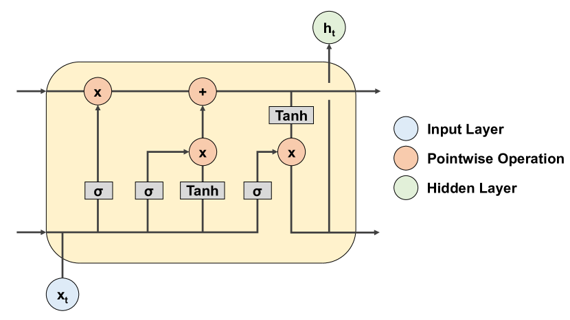
((a)) cnn model type.

((b)) mlp model type.

((c)) U-Net model type.

((d)) Autoencoder model type.

((e)) lstm model type.

((f)) gan model type.

Figure 3: Overview of the most commonly used model types that are discussed in this review. In 3(a) a cnn architecture is visualized which takes a spectrum as input and outputs scalar values (i.e. metabolite concentrations). In 3(b) a mlp is visualized with an arbitrary number of nodes. In 3(c) a U-Net model is visualized which performs super-resolution with a lrsi image as input and a hrsi image as output. In 3(d) a general autoencoder is visualized which aims to reconstruct the input spectrum in the output. In 3(e) a lstm model is visualized which takes a (time) sequence input and uses feedback connections to calculate the next hidden layer. Variables $x_{t}$ and $h_{t}$ indicate the sequence value and hidden state at timestep $t$ respectively. In 3(f) a gan model is visualized that generates artificial spectra using a generator and includes a discriminator to determine whether a spectrum is real or fake.

2 Data Acquisition

During data acquisition, scan-configuration parameters need to be optimized to get the desired and optimal data output. In this section some ml-based data acquisition methods are summarized and discussed.

2.1 Volume Selection

Voxel placement in svs (svs) is critical to limit partial volume effects, especially for the analysis of brain tumors. Bolan et al. ²² propose an algorithm for automated voxel placement. They use a dataset of 60 low grade glioma patients containing T2w flair (flair) images and corresponding mrs voxels manually placed by an expert spectroscopist. Lesion masks are retrospectively annotated by an experienced neurooncologist to have a gold-standard for training. The first step in their method involves tumor segmentation using a pre-trained cnn model that is fine-tuned with their own dataset. The obtained segmentation volumes are used to maximize an objective function that describes the placement of a cuboid voxel in terms of position, size and rotation angle. This function captures two main considerations: voxel size and lesion fraction. Evaluation is done by comparing the lesion fraction, the volume of intersection between the annotated lesion and the mrs voxel, and the total voxel size between manually and automatically placed voxels. The authors found that the proposed automatic placement method has a higher lesion fraction compared to manually placed voxels. Moreover, their method demonstrates more consistent placement with lower standard deviations for lesion fraction, volume of intersection, and voxel size.

2.2 Shimming

Performing $B_{0}$ shimming is important to obtain useful and high-quality mrs data ⁵. To accelerate and automate the shimming process, Becker et al. ²³ proposes a dl-based method for shimming. The used dataset contains raw ¹H-fid signals with shim offsets, in which only linear shims in orthogonal $X,Y$ and $Z$ directions are considered. The dl method aims to predict shim values for the $X,Y$, and $Z$ directions based on the 1d (1d) spectra of the linear shim offsets. They use an ensemble model architecture consisting of heterogeneous weak learners that are combined by either averaging, a fully connected layer, or a mlp. Results show that both a single weak learner and the ensemble model with a mlp are able to predict shim values that improve spectral quality. These models are also used in combination with the downhill simplex method ⁶⁴, which is well-established for automatic shimming. They found that using their models, as stand-alone or in combination with this simplex method, results in either a reduction in the number of acquisitions necessary or an improvement in spectral quality.

In a follow-up study, Becker et al. ²⁴ extend their previous work by incorporating a higher order shim ($Z^{2}$) and a different nn architecture in their study. The proposed architecture uses a cnn combined with a lstm block in order to mimic a signal-based shimming technique where the previously obtained states, in the form of a 1d spectrum and a shim offset, are used in the process. The value of the shim offsets are dependent on the time step during training. First, a number of random steps are taken followed by a series of predictive steps for which the input shim offsets are the previously obtained values. The results show that using dl methods, with or without traditional optimization algorithms, is more effective than using traditional optimization alone.

3 Processing

Raw mrs and mrsi measurements require a multitude of processing steps to obtain interpretable signals. Commonly recommended steps for mrs include coil combination, signal averaging, motion correction, eddy current correction, fpc (fpc), and identification of spurious echoes ⁷.The following sections present and summarize ml studies that have shown to improve and replace such existing processing methods.

3.1 Reconstruction

Efficient sampling and reconstruction techniques play an important role in accelerating mrs and mrsi methods. When the data is highly under-sampled, reconstructing spectra from truncated fid creates truncation artifacts. Lee et al. ²⁶ propose and compare three different reconstruction approaches with identically designed U-Net ⁶⁵ architectures. The networks differ based on their inputs and outputs, which are either completely in the time domain, completely in the frequency domain, or mixed (fid in, spectrum out). In-vivo 9.4T rat brain spectra are acquired to test the approaches as well as extract knowledge of the present snr and linewidth values. Training data is obtained using a basis set simulation for 17 metabolites. The results show that the U-Net operating purely in the frequency domain has the best performance in terms of lowest nmse (nmse) and highest Pearson correlation coefficient (for the simulated data). The following observations are made with the simulated data: for 8 and 16 retained points (out of 1024) the U-Net recovers spectra with substantial truncation artifacts; for 32 and 64 retained points the approach manages to recover spectra with minor residuals; for 128 (and upwards) the truncation artifacts are well suppressed by the nn, enabling precise quantification.

In addition to 1d svs there are 2d (2d) mrs techniques, such as the lcosy (lcosy) experiment ⁶⁶. Despite the long acquisition time for lcosy, it can aid in distinguishing overlapping metabolites. Luo et al. ²⁷ introduce an encoder-decoder network architecture for fast reconstruction of nus (nus) lcosy spectra by learning to predict fully-sampled spectra from under-sampled input spectra. They propose to use simulated training data generated by the mode of virtual echo ⁶⁷, where the under-sampled spectra are obtained by exponential and Poisson-gap sampling. This method is found to have fewer reconstruction artifacts and better peak preservation compared to other architectures such as cnn and U-Net. It is also further evaluated with multi-nuclei spectra and found to have similar reconstruction quality compared to an iterative soft thresholding approach ⁶⁸ as well as smile (smile) reconstruction ⁶⁹.

To accelerate lcosy experiments, Iqbal et al. ²⁸ propose a U-Net model to reconstruct fully-sampled spectra using nus spectra as an input. They test their approach on simulated lcosy spectra with exponential sampling. Results suggest that the U-Net architecture not only produces good quality spectra for all tested acceleration factors (1.3$\times$, 2$\times$, and 4$\times$), but also outperforms the compressed-sensing results of an $L1$-norm minimization method for the higher acceleration factors.

Various acceleration techniques have been explored for mrsi ^{70, 71}, mainly through under-sampling of the k-space and reconstruction using compressed-sensing or parallel imaging techniques ^{72, 73, 74}. Nassirpour et al. ²⁵ propose to improve the conventional grappa (grappa) reconstruction ⁷³ by estimating k-space weightings with multiple nn to reduce lipid aliasing. They train two types of single-layer nn to predict the missing data points; one for cross-neighbors and one for adjacent neighbors. During reconstruction, the two network types are deployed sequentially in such a way that first the cross-neighbor nn fill in the missing k-space values and then the adjacent-neighbor nn estimate the remaining points. Additionally, the authors propose variable density under-sampling schemes to achieve even higher acceleration factors and alter their ml framework by first using 2-voxel cross-neighbor and adjacent-neighbor nn before using the previously mentioned 1-voxel neighbor nn. Although in this work the networks are trained in a subject-specific manner, various strategies are investigated in  ³⁰ to improve this approach with more samples. The results suggest the use of nn for grappa reconstruction reduces aliasing artifacts thereby positively impacting metabolite concentration maps and significantly boosting the performance compared to regular grappa.

Furthermore, Motyka et al. ²⁹ proposes a k-space-based coil combination using geometric dl to reduce the amount of processing data immediately after the acquisition instead of reducing the data in the image domain. Their approach utilizes a shallow-graph nn ⁷⁵ to learn the k-space representation of the mrsi data before the summation step of the coil combination. In-vivo data are augmented for training and pairs consisting of input and desired output for each partition encoding step and each fid point are created. Additionally, white Gaussian noise is added to the training samples to increase the robustness of the method. The proposed method is compared to the conventional image-based coil combination iMUSICAL ⁷⁶. For both approaches, the metabolite concentration maps are similar to the crlbp of LCModel ⁷⁷. The proposed method performs comparable to iMUSICAL when evaluated for different snr levels, slightly under-performing for high snr domains.

3.2 Spectral Denoising

svs acquisition time linearly depends on the number of signal averages which are obtained to enhance the snr. Learning the mapping between low nsa (nsa) spectra to high nsa spectra can effectively denoise and improve the snr of the mrs signal.

Lei et al. ³¹ propose an autoencoder model to denoise mrs spectra. For that purpose they acquire multiple phantom and in-vivo spectra with a nsa of 192 and of 8, representing high and low snr. The proposed network consists of an encoder-decoder architecture, taking the processed low nsa spectra as the input in the frequency domain and outputting high nsa spectra with reduced noise. To enlarge the data variability a patch-based input is used in combination with data augmentation. The network is optimized using the mse (mse) of the output spectra and the gt (gt) high snr spectra including a $L1$-norm on the hidden feature vector to enforce sparsity. snr estimates of the input and output spectra show an snr improvement of 40% and 47% for phantom and in-vivo data, respectively, showing potential to accelerate mrs acquisitions by acquiring low nsa spectra while maintaining spectral quality.

3.3 Super-Resolution MRSI

Long acquisition times and high field strengths are often necessary to obtain hrsi (hrsi) data. Advanced post-processing methods to increase the resolution for lrsi (lrsi) data can be beneficial for reaching the desired resolution. Iqbal et al. ³² propose a supervised dl method for super-resolution of mrsi data. They propose a U-Net architecture to take a T1w image and corresponding lrsi image as inputs and produce a hrsi image as output. In total, three different U-Nets are trained for three different lrsi resolutions (16x16, 24x24 and 32x32). They use synthetic data, generated by a mrsi simulator, for training and testing. This generator produces T1w images and a pair of lrsi and hrsi data. The synthetic data is used to evaluate the trained models based on the mse of the hrsi reconstructions and the reconstruction of individual spectra at different resolutions. Additionally, the models are tested on downsampled in-vivo hrsi data. During evaluation, different noise levels are tested and a comparison is performed with standard methods like zero-filling and bicubic interpolation. Results show that the dl method performs better than standard methods for all noise levels and can be used as a denoising or acceleration method.

In a follow-up study, Dong et al. ³³ propose another super-resolution model which included in-vivo mri and mrsi data. A dataset of hrsi (64$\times$64) data is acquired and down-sampled to obtain lrsi (16$\times$16) data. In total, 320 metabolic maps from 3 different patients are used as gt. The dl method consists of a U-Net with four different input modalities: lrsi data, T1-weighted images, flair images and contrast-enhanced T1-weighted images. The decoding part of the network uses spatial attention modules which automatically calculate spatial weight maps to focus on important features in each input modality. The hrsi output is used to calculate the loss function, which consists of three different parts. The first part is a pixelwise mse loss, calculated by comparing the output with the gt data. To account for inter-pixel correlations, a second term called the ms-ssim (ms-ssim) is added. The ms-ssim measures the similarity between two different images at multiple scales in terms of luminance, contrast and structure. Finally, a discriminator is added to calculate an adversarial loss and capture more complex features. This study investigates the contribution of all different loss terms and input modalities by training multiple models. Results show that including all aforementioned inputs and losses achieves the best performance, also out-performing standard bi-cubic interpolation.

3.4 Frequency & Phase Correction

fpc is necessary to reduce the effects of scanner frequency drifts, subject motion, or other inconsistencies to ensure reliable quantification without line broadening or loss in snr. This is especially crucial in J-difference edited mrs spectra which rely on accurately subtracting two aligned spectra.

Tapper et al. ³⁴ propose an automated fpc framework consisting of two separate nn. A simulated dataset set is obtained using ideal excitation/refocusing pulses and shaped editing pulses. The simulation parameters are chosen to match the in-vivo data (Big GABA repository ⁷⁸) as close as possible. Both corrections are implemented with two sequentially placed fully connected nn, where the frequency shifts are estimated first, followed by an estimation of the phase offsets. Both models are trained individually taking the magnitude or real-only spectra, respectively, as the input to predict the frequency or phase offsets. Results for simulated test data show accurate predictions with a mean frequency offset error reported at $0.00\pm 0.03$ Hz and a mean phase offset error of $-0.11\pm 0.25$ degrees. Evaluation with in-vivo data shows similar performance to a model-based sr (sr) method ⁷⁹, however, they indicate a substantial performance degradation compared to the simulated data.

Based on this work, Ma et al. ³⁵ propose an alternative dl approach for fpc using cnn architectures. They use identical parameter configurations to simulate MEGA- press (press) data for training and validation. However, they create additional spectra with lower snr by adding Gaussian noise. The authors observe less subtraction artifacts with the cnn and show an overall better performance than the approach of Tapper et al.³⁴. For the simulated data the authors report a mean frequency offset error of $0.02\pm 0.02$ Hz for the mlp and $0.01\pm 0.01$ Hz for the cnn, and a mean phase offset error of $0.19\pm 0.17$ degree for the mlp and $0.12\pm 0.09$ degree for the cnn. For the in-vivo scenarios, performance is measured based on the variance of the choline metabolite of the spectra subtraction. The cnn performs better in 66.67% , 60.61%, and 75.76% of the 33 datasets, when small, medium, and large offsets are added to the data, respectively.

Shamaei at al. ³⁶ develop unsupervised methods for fpc including two different cemd (cemd) models in which the input spectra are used as targets during training. One model focuses on reference peak fitting of cr and uses a convolutional encoder to construct a lower dimensional latent representation of the input. The latent parameters are used as input for a Lorentzian lineshape model decoder. The second cemd model uses the same encoder, but a sr function is used as decoder. To account for unstable frequency components, both models are also trained for a limited frequency range (2.5 to 3.5 ppm). Training and validation is done on a simulated dataset with known frequency and phase offsets and evaluation is done on phantom data and in-vivo data from the Big GABA repository. The proposed unsupervised methods are compared with commonly used fpc methods (sr and cr referencing, both on full and limited frequency ranges) and previous dl methods ^{34, 35}. In contrast to the non-dl fpc methods, the cemd models perform equally well when trained and applied on a limited frequency range and their performance is less influenced by the presence of nuisance peaks. Compared to the previous dl methods, the cemd is able to train in an unsupervised fashion and requires only one network for both frequency and phase correction.

3.5 Ghosting Artifact Removal

Ghosting artifacts, or so-called spurious echos, are usually caused by insufficient spoiling gradient power in combination with local susceptibility variations. These artifacts negatively influence the reliability of metabolite quantification as they may overlap with metabolite peaks.

Kyathanahally et al. ³⁷ evaluate two networks based on fully connected nn and cnn for the detection as well as an autoencoder network with residual blocks for the removal of ghosting artifacts. Brain metabolite spectra are simulated for ideal press characteristics, and ghosting artifacts with varying line-widths and amplitudes are added randomly. The fully connected nn is trained on 1d spectra as input and class probabilities as output. An alternative classification approach is implemented with a cnn, taking the real and imaginary part of a 2d spectrogram as input. The spectrograms are obtained by segmenting the time domain signals followed by a Fourier transform of each segment, creating 2d time-frequency spectrograms. To effectively remove the ghosting artifacts, an autoencoder network is implemented, taking the 2d corrupted spectrograms as input and outputting artifact-free spectrograms. The authors report a classification accuracy between 50% and 75% for the fully connected nn depending on the number of layers. In contrast, the cnn approach shows promising performance with a mean accuracy of 94% for smaller datasets and an accuracy of over 99% for larger training sets and subsequent in-vivo evaluations. In addition, the autoencoder method is found to be effective in removing ghost artifacts from distorted spectra, with low rmse (rmse) reported for the difference between ground truth and restored spectra in simulated data. However, the restoration is found to be suboptimal for in-vivo cases.

3.6 General Artifact Removal

The previously discussed methods all focus on a specific processing step, yet nn have the ability to learn more complex mappings from training data, enabling multiple artifact corrections at once. Lee and Kim ³⁸ propose a cnn architecture taking spectra contaminated with artifacts as input and predicting noise-free, metabolite-only spectra. The nn is trained using simulated data with metabolite phantom spectra as a basis set and knowledge of in-vivo data for specific linewidth, snr, and baseline ranges. Further, in-vivo test data is obtained from five healthy volunteers with identical scanner settings used for the phantom spectra of the basis set. For both simulated and in-vivo data, the cnn clearly manages to obtain spectra with removed noise, narrow linewidth, removed frequency and phase shifts, and without spectral baseline. The results show no visible residual signal and thus suggest good removal of artifacts only in the simulated scenario. Further, the reported mape of the quantification estimates and the gt concentrations is $20.67\%\pm 16.71\%$. For the in-vivo spectra the results of the proposed method coincide with estimates of LCModel as well as commonly reported metabolite concentrations from the literature.

4 Analysis

The mrs analysis focuses on converting the (processed) signals into meaningful and reliable metabolite concentration estimates. The following subsections summarize recent ml applications for spectral quality assurance, metabolite quantification, uncertainty measurement, and classification.

4.1 Quality Assurance

mrs and mrsi methods are susceptible to various imperfections causing artifacts in the acquired spectra which in turn can create unreliable and inaccurate measurements. This is limiting the clinical use of mrs and causes a dependence on technical experts to inspect the spectral quality.

De Barros et al. ³⁹ introduce an active learning method to improve labeling efficiency based on spectral quality by either accepting or rejecting spectra for further analysis. The method uses a dataset of over 28,000 in-vivo spectra from brain tumor patients. Forty-seven features are extracted from the time-domain and frequency-domain magnitude spectra and are used as input for a rf (rf) classifier. Two expert spectroscopists manually label the spectra to provide gt for supervised training. The active learning strategy employs an uncertainty range defined as $[0.5-\alpha,0.5+\alpha]$, where $\alpha$ controls the width. When the rf classifier’s output falls within this range, the uncertain data instance is added to the training set. This active learning method is evaluated iteratively, where in each iteration spectra from one patient are evaluated and uncertain examples are added to the training set. After retraining, the rf classifier is validated on one patient (leave-one-out-cross-validation). Results show insignificant or minor differences in classification performance between different values for $\alpha$ ($0.1\leq\alpha\leq 0.5$), resulting in an efficient way of training a rf classifier with fewer manual labeling.

Gurbani et al. ⁴⁰ propose a cnn architecture to automatically classify the quality of a given spectrum and integrate it into a software pipeline enabling real-time filtering of epsi (epsi) data. In-vivo spectra from patients with glioblastoma are collected after appropriate filtering. These spectra are then reviewed by mrs experts and classified as ”Good”, ”Acceptable”, or ”Poor” quality to obtain gt labels for the nn. The cnn architecture takes the normalized real component of the spectrum as input and splits it into six specific regions, each with its own designated cnn. These cnn are trained in parallel by passing their concatenated outputs through a mlp of which the output represents the probability to be classified as ”Good”. The overall model performs well in terms of detecting ”Poor” quality spectra with an auc (auc) of 0.951.

Kyathanahally et al. ⁴¹ evaluate various ml approaches for fast quality classification of mr spectra. The authors perform training and testing on the multi-center studies INTERPRET ⁸⁰ and eTUMOUR ⁸¹ consisting of more than 1000 spectra, mostly already classified into good and bad quality. Furthermore, they create an intermediate class for ”Poor” quality if one of the three experts thought the spectrum was acceptable, and they also create their own local expert ratings for some previously unlabeled data. The authors evaluate various classifiers based on svm, lda (lda), and rusboost (rusboost) in combination with ica (ica) and pca (pca) or sffs (sffs) and tree (tree) as feature extraction or feature selection methods. Their final approach uses a high number of features as input and a rusboost classifier that undersamples to combat the imbalanced training data, showing a comparable performance in rejecting unsuitable spectra to a human expert.

Hernández‐Villegas et al. ⁴³ propose a cnmf (cnmf) for the same multi-center studies used in ⁴¹ to distinguish between good and poor quality spectra. The method first iteratively factorizes observations into a source matrix (of data centroids) and a mixing matrix (containing combination weights). Then, two experts define quality measures based on correlation and Euclidean distance of the extracted sources of 10 repetitions as well as based on the coding coefficient of the mixing matrices. Thereby, spectral quality can be assessed and characterized in an unsupervised fashion. The obtained results indicate that the defined quality measures can identify sources containing artifacts and the approach manages to distinguish between good and poor-quality spectra.

Jang et al. ⁴² train a gan to detect abnormalities in 3T human brain spectra. Normal and abnormal brain spectra are simulated, similarly to Lee and Kim ³⁸. Eight different classes of spectra are generated that are abnormal in snr, linewidth, a single metabolite concentration, multiple metabolites concentrations (9), or all factors combined. Additionally, spectra that contain ghosting, residual water, or residual lipid artifacts are simulated with the help of phantom data. After training the gan on normal spectra only, latent space mapping is performed. This mapping is done with a loss function containing a dissimilarity term that compares the generator output with the input spectra, and a discriminator term that uses feature matching from the second last layer of the discriminator. The classification between normal and abnormal spectra is performed with a 2d threshold using nmse and the standard deviation of the spectra. Results show over 80% accuracy for some abnormalities such as snr and naa concentration. Additionally, the gan also detects ghosting, residual water, and residual lipid artifacts without using those spectra in the training phase. However, the model cannot accurately detect abnormalities in linewidth and low-concentrated metabolites with accuracies of around 50%.

4.2 Quantification

Quantification aims at converting processed mrs spectra/fid into specific metabolite concentration estimates. Traditionally, model-based methods employed for metabolite quantification include linear combination model fitting, peak fitting, and peak integration ^{82, 83}.

An early ml-based quantification approach is introduced by Das et al. ⁴⁴ where they propose a rf regression method. The proposed model is developed with different combinations of artificial spectra and in-vivo spectra. The rf consists of a set of binary trees with splits based on random subsets of the feature variables on which the forest is subsequently trained. The trees of the rf are trained using piece-wise linear regression over the input spectrum outputting metabolite concentration estimates, followed by taking the weighted average of the predictions from each tree to obtain a single output estimate. Results show that the rf technique has similar performance as LCModel and could therefore be used in combination with LCModel to assist with the quantification of noisy spectra and enable faster convergence.

Hatami et al. ⁴⁵ propose a supervised cnn model for metabolite quantification which is able to cover 20 different metabolites and a macromolecule signal. The cnn takes real and imaginary parts of the spectra as a two-channel input and outputs concentrations of all metabolites of interest. A training and test with gt concentrations are obtained by simulating spectra based on an mrs signal model. To evaluate the accuracy of the quantification model, the smape (smape) over the whole test set is calculated and compared with the performance of the model-based QUEST ⁸⁴ method and the previously mentioned rf regression algorithm from Das et al. ⁴⁴. The proposed cnn outperforms the other methods with and without the addition of noise.

Shamaei et al. ⁴⁸ investigate the use of a cnn which used a wavelet scattering transformation to extract features from the mrs signal. The extracted features are fed into a fully connected feed-forward nn to predict the relative amplitudes of the metabolite basis spectra, which can be used for absolute quantification. For training and evaluation, multiple datasets are simulated by using a signal-based model and uniform sampling of its parameters. Their model shows better performance, in terms of smape, compared to QUEST and similar performance as the model of Hatami et al. ⁴⁵. Additionally, the wavelet scattering cnn shows robustness against metabolite phase changes and nuisance signals, such as macromolecules.

Gurbani et al. ⁴⁶ use a cemd for spectral fitting. This two-step unsupervised dl approach takes the real part of the spectrum as an input. During the first encoder-decoder step, a spectrum is mapped to a lower-dimensional space and a baseline is reconstructed using a wavelet reconstruction decoder. The resulting baseline is subtracted from the input spectrum and fed into the second encoder-decoder network, which is used to reconstruct the spectral lineshape, and therefore the fitting parameters for the metabolites of interest. Three metabolites are considered including cho (cho), cr, and naa. The final cemd model is also included in a pipeline for creating whole-brain metabolite maps for patients with glioblastoma and is compared with MIDAS ⁸⁵. Results show that both methods have similar fitting performance and the cho/naa maps created by the cemd have a Dice score of 0.72 when compared to MIDAS.

Lee and Kim ⁴⁷ propose a cnn architecture to quantify metabolite concentrations. Their approach consists of a designated cnn per metabolite, taking the real part of a spectrum as input to estimate the corresponding metabolite spectrum. The actual quantification of the metabolites is then obtained by computing the areas of the known spectral regions relative to the methyl signal of tcr (tcr). The results for the proposed quantification approach show a well-performing algorithm for the completely synthetic scenarios (i.e. mape of 1.92% and 2.56% for the methyl ($\sim 3.0$ ppm) and methylene ($\sim 3.9$ ppm) peaks for the reference metabolite tcr). For the simulated spectra using metabolite phantoms and in-vivo baselines the mean mape is increased as depicted above and ranged from $14.79\pm 11.12\%$ to $23.07\pm 16.36\%$ over the major metabolites.

Similarly, Iqbal et al. ²⁸ propose a method with a designated nn per metabolite implemented using U-Nets. Their approach takes the real, imaginary, and magnitude information of a fully sampled lcosy spectrum as input and outputs the magnitude spectrum for each of the seventeen metabolites. The authors observe an increase in error for both degrading snr and higher water signal amplitude. Nonetheless, the model shows accurate quantification of the metabolites, even for low concentrations.

Rizzo et al. ⁴⁹ compare mrs quantification using various cnn models, input types, and learning methods. They use a simulated artifact-free dataset with gt concentrations to enable fair comparison with standard model fitting. Results indicate that 2d spectrogram inputs outperform 1d frequency domain inputs and that including a water reference peak improves performance. The best model is a heterogeneous ensemble combining 1d and 2d inputs while increasing dataset size and applying active learning strategies do not significantly improve performance. However, dl-based quantification still underperforms compared to standard model fitting and is highly biased toward training data when snr is low.

Schmid et al. ⁵⁰ propose a dl-based peak detection method as part of classical peak fitting. A simulated dataset, including various distortions, is used for training. Their cnn model with lstm blocks outputs classes (baseline, narrow peak, or broad peak) and values for the peak widths. Input spectra are dynamically scaled to enhance local contrast and peak labels are acquired with an automatic labeling procedure. The outputs are used to fix the number of peaks and initialize the peak width values for a classical peak fitting algorithm. Evaluations on simulated and experimental data show high scores on picking accuracy, spectral reconstruction, and sparsity of the peak selection. Their method outperforms using manual peak picking in terms of mae (mae), especially in crowded regions (i.e. $82$% lower mae). The authors state that their method, although optimized for high-field proton spectroscopy, is adaptable to different domains.

Shamaei at al. ⁵¹ implements a physics-informed dl method to quantify simulated spectra and in-vivo spectra from the Big GABA repository ⁷⁸. They use a cemd architecture with an encoder that outputs parameters for the signal-based model decoder. This decoder uses a metabolite basis set and a numeric, parameterized, or regulated parameterized mm (mm) signal contribution as prior knowledge. Their experiments include the investigation of different architectures for the encoder, the use of different mm models, and different dataset sizes. Results show comparable performance to traditional quantification methods and the ability to use this dl approach for in-vivo data, with best performances for shallow cnn encoders and minimum dataset sizes of 12,000 samples. Additionally, a numerical mm signal is favorable above parameterized and regulated parameterized mm models. Due to the unsupervised training approach and the significant reduction in computation time, this method could be used as a faster alternative to quantify large, in-vivo mrs datasets.

4.3 Uncertainty Measurement

Uncertainty measurements of metabolite concentration estimates, such as the crlb (crlb) or the crlbp are crucial for assuring reliable results, yet for data-driven methods such measures are generally biased and alternative metrics are difficult to validate.

Lee and Kim ⁴⁷ propose a cnn-based approach to quantify metabolite concentrations and simultaneously obtain an uncertainty estimate for the output spectra. The approach is developed with simulated rat brain spectra and is further evaluated using phantom data and in-vivo rat brain spectra. The authors obtain a measurement uncertainty with respect to snr, linewidth, and sbr (sbr) by constructing an uncertainty measurement database from the training data. The snr and linewidth are estimated from the input spectrum, specifically from tnaa (tnaa), while the sbr of each metabolite is measured from the predicted metabolite spectra. Then a 3d (3d) space of the quantitative errors is computed and stored for each target metabolite as a function of the snr, linewidth, and sbr. The estimated quantification uncertainty of the proposed method is highly correlated with the actual errors obtained in a purely simulated scenario (i.e. $0.81\pm 0.13;0.88\pm 0.09$ for 15 major metabolites). The correlation predicted error and gt error for the simulated spectra using metabolite phantoms and in-vivo baselines are slightly lower (i.e. 0.7 or higher ($0.78\pm 0.05$) and statistically significant for all 15 major metabolites).

In another work of Lee and Kim ⁵², they propose an alternative cnn architecture and training procedure to obtain both an estimate of metabolite concentrations and their uncertainties. Using mcdo (mcdo) ⁸⁶ and a variance leveraging loss function based on the log-likelihood ⁸⁷ both epistemic (model) and aleatoric (data) uncertainty estimates are obtained for each metabolite concentration. The cnn is trained with simulated spectra, further tested with in-vivo data, and shows comparable performance to model-based alternatives such as LCModel.

The work of Rizzo et al. ⁵³ investigates the reliability of dl-based quantification and compared it to common model fitting methods. For that purpose, they design a cnn taking spectrograms as input and outputting normalized metabolite concentration estimates. In a similar fashion to Lee et al. ⁵² the authors use mcdo for epistemic (model) uncertainty and metrics based on bias and spread of the predicted concentration distribution for aleatoric (data) uncertainty information. The results indicate that the cnn’s predictions tend towards the mean of the test data in cases with high uncertainty, indicating the model is biased. Meanwhile, model fitting methods show on average to be unbiased.

4.4 Classification

Classification in mrs and mrsi data is important for clinical applications in terms of diagnosis and disease monitoring. Instead of using metabolite concentrations, ml methods can be trained to perform direct classification.

In a multi-class pediatric brain tumor classification problem, Zarinabad et al. ⁵⁴ show that various ml methods can distinguish between three different tumor classes. An unbalanced dataset (in-vivo, 1.5T) is used in combination with bsmote (bsmote) (based on the smote (smote) algorithm ⁸⁸) to increase classification performance. The trained classifiers consist of a rf classifier with an adaptive number of trees and four different AdaBoostM1 algorithms using different weak learners: naive Bayes, svm, nn and lda. Classification is done by either using the full spectra or the metabolite concentrations quantified by TARQUIN ⁸⁹. Oversampling the minority class with bsmote results in better classification performances of the trained classifiers, both for concentrations and spectral inputs. The best balanced accuracy rates are $0.93$ and $0.90$ for concentrations and spectral inputs respectively, with different combinations of classifiers and oversampling rates possible.

A similar classification problem is investigated in a subsequent study from Zarinabad et al. ⁵⁵. However, the spectra are acquired on 3T scanners from four different hospitals. The tested classification algorithms are lda, svm and rf approaches and bsmote is used to account for the class imbalance. pca is performed on the metabolite profiles to extract four principal components which are used as input for the classification algorithms. The results show a maximum balanced accuracy of $0.86$ when using svm as a classification method, which compares favorably with a previous 1.5T multi-center study ⁹⁰.

For the same multiclass tumor classification, Zhao et al. ⁵⁷ propose to add metabolite selection. This study compares pca and multiclass roc (roc) as metabolite selection methods for training ml classifiers: lda, $k$-nearest neighbors, naive Bayes, nn and svm. The classification with three tumor classes is done for both 1.5T and 3T svs data from multiple sites and oversampling for minority classes is done using the smote algorithm. Final classification accuracy is determined using $k$-fold and leave-one-out cross-validation. Metabolite selection using multiclass roc shows a higher accuracy compared to pca with the highest balanced classification accuracy of 85% for the 1.5T data with svm and 75% for the 3T data with lda. A more transparent and explainable tool for diagnosis is obtained by selection of metabolites for ml-based classification.

Dikaios ⁵⁶ trains three different ml methods to differentiate metastasis from glioblastoma brain tumors. The models include svm, mlp, and cnn. Different versions of the models with varying hyperparameters and/or layers are tested on four different datasets consisting of real GE spectra with additional noise, real Philips spectra with additional noise, synthetic GE spectra, and synthetic Philips spectra. A total of 12 models are trained using long TE, short TE, and concatenations of both versions of the spectra. Evaluation of the results, in terms of roc-auc and accuracy, shows the best performance for the 1d cnn when using synthetic data and the concatenated echo times ($>90\%$ accuracy).

5 Artificial Data Generation

Accessing in-vivo mrs/mrsi data is limited due to time-consuming acquisitions, non-standardized methods ⁹¹, and privacy concerns. To overcome this limitation, artificial data generation is used for developing ml applications. All previously discussed studies, containing artificial data, use non-ml based generation methods like data augmentation and model-based simulation. Data augmentation is a method that artificially increases the size and variety of the used dataset by applying transformations to real samples. On the other hand, model-based simulation involves sampling the parameters of a parametric model to generate mrs data, which is essentially an inverse use of signal-based fitting models. While the concepts of artificial data generation are the same, the exact implementation varies a lot per study.

ml methods can also be applied for artificial data generation itself. The work of Olliverre et al. ⁵⁸ focuses on generative models for creating mrs spectra. This study compares three different models (gan, dcgan (dcgan), and pmm (pmm) ⁹²) on their ability to generate mrs spectra for three classes: healthy, low-grade and high-grade tissue. The models are trained on a dataset consisting of 137, 1.5T press acquired in-vivo spectra. The gan model uses a generator and discriminator with fully connected layers and the dcgan uses a deeper architecture, which generally requires more data. The dcgan is therefore trained by using the full training dataset as batch size with the addition of batch normalization to deal with the relatively small dataset. All models are trained on all three tissue types separately and the quality of the artificially generated data is tested by training a rf classifier. Results show that datasets generated by the gan and pmm are able to train a rf classifier to the same level as using real mrs data. The dcgan generated data has lower performance due to the small dataset size that underutilizes the potential of deep learning.

6 Conclusion & Outlook

This review highlights recent ml studies within the field of proton mrs, focusing primarily on processing and analysis of mrs spectra and mrsi images with less attention on data acquisition. Although some studies have applied ml to volume selection for svs and shimming, other aspects of data acquisition (e.g., pulse sequence design, suppression techniques, and excitation area) have so far been disregarded. Due to the hardware-dependent nature of such applications, they are not only more difficult to integrate, but also to develop and test. Meanwhile, topics like quality assurance, quantification, and classification are more commonly addressed. Through the ability to simulate processed spectra or to rely on large databases for training data, such ml models are more straightforward to develop. In the future, more acquisition-oriented simulations could bridge this gap.

Recent ml studies focus on dl model types instead of classical ml methods like svm, rf, lda, or pca. Table 1 reveals that the most commonly used model type is a cnn. Additionally, most autoencoders, U-Nets, and ensemble model types also include convolutional layers. cnn are widely adapted in computer vision and medical imaging ^{93, 94} with their benefits of weight sharing, simultaneously extracting features and performing classification, and easy implementation into large-scale networks ⁹⁵. While recent studies from Rizzo et al. ⁴⁹ and Shamaei et al. ⁵¹ compare different model architectures, more comparison studies are still missing. Future work should focus on testing different and new model types like transformers that have shown potential in other medical imaging fields ⁹⁶. These types of studies can aid in finding the best practices for mrs and mrsi applications. As the field of ml rapidly evolves, it is important to keep up-to-date with new developments and investigate their role in mrs and other spectroscopy domains.

Section 5 mentions that many studies use different techniques to generate artificial data to develop their ml methods, making the comparability between different studies very challenging. Also, significant performance drops are observed when models are trained with artificial data and tested on in-vivo data, showing difficulties in transferability from artificial data to in-vivo data. This stems not only from lacking generalization capabilities of the ml methods, but also from the difficulty of accurately replicating in-vivo data through simulation or synthesis. While metabolite signals are well understood using density matrix simulations, other signal contributions, like macromolecules, water/fat residuals, and other artifacts, remain challenging to simulate. Therefore, efforts that investigate and standardize (artificial) data generation, as well as augmentation techniques, are crucial for future research.

ml methods rely on their training data to learn meaningful tasks and are inherently biased towards this data. Without preventive or predictive measures there are no guarantees for the model’s performance for inputs outside of this distribution ⁹⁷. Furthermore, the model’s output might even collapse to the mean of its target distribution for mismatched inputs ⁹⁷. In a clinical setting, such behaviors need to be detected and removed. Reliable and broadly applicable uncertainty measures for ml prediction are therefore crucial for or clinical applicability of ml in mrs. Additionally, deploying hybrid models (combined model-based and data-driven systems) can allow ml contributions to be leveraged by physics-informed models that behave unbiased and have guarantees on their estimates ⁹⁸.

The clinical utility of ml applications in mrs and mrsi is one of the most important aspects of this research field. Attempts to decrease human-expert involvement, decrease acquisition time, and increase robustness and generalizability of existing mrs tools are therefore essential. ml methods should also be easy to interpret by clinicians to be useful in clinical workflows. While ml in mrs and mrsi is still in the early stages, the discussed studies show great potential for clinical adoption with plenty of future research possibilities.

References

- 1 Buonocore Michael H., Maddock Richard J.. Magnetic Resonance Spectroscopy of the Brain: A Review of Physical Principles and Technical Methods. Reviews in the Neurosciences. 2015;26(6):609–632.
- 2 Faghihi Reza, Zeinali-Rafsanjani Banafsheh, Mosleh-Shirazi Mohammad-Amin, et al. Magnetic Resonance Spectroscopy and Its Clinical Applications: A Review. Journal of Medical Imaging and Radiation Sciences. 2017;48(3):233–253.
- 3 Wilson Martin, Andronesi Ovidiu, Barker Peter B., et al. Methodological Consensus on Clinical Proton MRS of the Brain: Review and Recommendations. Magnetic Resonance in Medicine. 2019;82(2):527–550.
- 4 Landheer Karl, Schulte Rolf F., Treacy Michael S., Swanberg Kelley M., Juchem Christoph. Theoretical Description of Modern 1H in Vivo Magnetic Resonance Spectroscopic Pulse Sequences. Journal of Magnetic Resonance Imaging. 2020;51(4):1008–1029.
- 5 Juchem Christoph, Cudalbu Cristina, de Graaf Robin A., et al. B0 Shimming for in Vivo Magnetic Resonance Spectroscopy: Experts’ Consensus Recommendations. NMR in Biomedicine. 2021;34(5):e4350.
- 6 Jansen Jacobus F. A., Backes Walter H., Nicolay Klaas, Kooi M. Eline. 1H MR Spectroscopy of the Brain: Absolute Quantification of Metabolites. Radiology. 2006;240(2):318–332.
- 7 Near Jamie, Harris Ashley D., Juchem Christoph, et al. Preprocessing, Analysis and Quantification in Single-Voxel Magnetic Resonance Spectroscopy: Experts’ Consensus Recommendations. NMR in Biomedicine. 2021;34(5):e4257.
- 8 Knoll Florian, Hammernik Kerstin, Zhang Chi, et al. Deep-Learning Methods for Parallel Magnetic Resonance Imaging Reconstruction: A Survey of the Current Approaches, Trends, and Issues. IEEE Signal Processing Magazine. 2020;37(1):128–140.
- 9 Montalt-Tordera Javier, Muthurangu Vivek, Hauptmann Andreas, Steeden Jennifer Anne. Machine Learning in Magnetic Resonance Imaging: Image Reconstruction. Physica Medica. 2021;83:79–87.
- 10 Pal Arghya, Rathi Yogesh. A Review and Experimental Evaluation of Deep Learning Methods for MRI Reconstruction. The Journal of Machine Learning for Biomedical Imaging. 2022;1:001.
- 11 Zhu Guangming, Jiang Bin, Tong Liz, Xie Yuan, Zaharchuk Greg, Wintermark Max. Applications of Deep Learning to Neuro-Imaging Techniques. Frontiers in Neurology. 2019;10:869.
- 12 Mohammed Bakhtyar Ahmed, Al-Ani Muzhir Shaban. Review Research of Medical Image Analysis Using Deep Learning. UHD Journal of Science and Technology. 2020;4(2):75–90.
- 13 Uddin L Q, Dajani D R, Voorhies W, Bednarz H, Kana R K. Progress and Roadblocks in the Search for Brain-Based Biomarkers of Autism and Attention-Deficit/Hyperactivity Disorder. Translational Psychiatry. 2017;7(8):e1218-e1218.
- 14 Rashid Barnaly, Calhoun Vince. Towards a Brain-based Predictome of Mental Illness. Human Brain Mapping. 2020;41(12):3468–3535.
- 15 Pilmeyer Jesper, Huijbers Willem, Lamerichs Rolf, Jansen Jacobus F. A., Breeuwer Marcel, Zinger Svitlana. Functional MRI in Major Depressive Disorder: A Review of Findings, Limitations, and Future Prospects. Journal of Neuroimaging. 2022;32(4):582–595.
- 16 Santana Caio Pinheiro, de Carvalho Emerson Assis, Rodrigues Igor Duarte, Bastos Guilherme Sousa, de Souza Adler Diniz, de Brito Lucelmo Lacerda. Rs-fMRI and Machine Learning for ASD Diagnosis: A Systematic Review and Meta-Analysis. Scientific Reports. 2022;12(1):6030.
- 17 Chen Dicheng, Wang Zi, Guo Di, Orekhov Vladislav, Qu Xiaobo. Review and Prospect: Deep Learning in Nuclear Magnetic Resonance Spectroscopy. Chemistry – A European Journal. 2020;26(46):10391–10401.
- 18 Rajeev S.K., Rajasekaran M. Pallikonda, Krishna Priya R., Al Bimani Ali. A Review on Magnetic Resonance Spectroscopy for Clinical Diagnosis of Brain Tumour Using Deep Learning. In: :461–465; 2021.
- 19 Wang Xizhao, Zhao Yanxia, Pourpanah Farhad. Recent Advances in Deep Learning. International Journal of Machine Learning and Cybernetics. 2020;11(4):747–750.
- 20 Marcus Gary. The Next Decade in AI: Four Steps Towards Robust Artificial Intelligence. 2020.
- 21 Sarker Iqbal H.. Deep Learning: A Comprehensive Overview on Techniques, Taxonomy, Applications and Research Directions. SN Computer Science. 2021;2(6):420.
- 22 Bolan Patrick J., Branzoli Francesca, Di Stefano Anna Luisa, et al. Automated Acquisition Planning for Magnetic Resonance Spectroscopy in Brain Cancer. In: Martel Anne L., Abolmaesumi Purang, Stoyanov Danail, et al. , eds. Medical Image Computing and Computer Assisted Intervention – MICCAI 2020, Lecture Notes in Computer Science:730–739Springer International Publishing; 2020; Cham.
- 23 Becker Moritz, Jouda Mazin, Kolchinskaya Anastasiya, Korvink Jan G.. Deep Regression with Ensembles Enables Fast, First-Order Shimming in Low-Field NMR. Journal of Magnetic Resonance. 2022;336:107151.
- 24 Becker Moritz, Lehmkuhl Sören, Kesselheim Stefan, Korvink Jan G., Jouda Mazin. Acquisitions with Random Shim Values Enhance AI-driven NMR Shimming. Journal of Magnetic Resonance. 2022;345:107323.
- 25 Nassirpour Sahar, Chang Paul, Henning Anke. MultiNet PyGRAPPA: Multiple Neural Networks for Reconstructing Variable Density GRAPPA (a 1H FID MRSI Study). NeuroImage. 2018;183:336–345.
- 26 Lee Hyochul, Lee Hyeong Hun, Kim Hyeonjin. Reconstruction of Spectra from Truncated Free Induction Decays by Deep Learning in Proton Magnetic Resonance Spectroscopy. Magnetic Resonance in Medicine. 2020;84(2):559–568.
- 27 Luo Jie, Zeng Qing, Wu Ke, Lin Yanqin. Fast Reconstruction of Non-Uniform Sampling Multidimensional NMR Spectroscopy via a Deep Neural Network. Journal of Magnetic Resonance. 2020;317:106772.
- 28 Iqbal Zohaib, Nguyen Dan, Thomas Michael Albert, Jiang Steve. Deep Learning Can Accelerate and Quantify Simulated Localized Correlated Spectroscopy. Scientific Reports. 2021;11(1):8727.
- 29 Motyka Stanislav, Hingerl Lukas, Strasser Bernhard, et al. k-Space-based Coil Combination via Geometric Deep Learning for Reconstruction of non-Cartesian MRSI Data. Magnetic Resonance in Medicine. 2021;86(5):2353–2367.
- 30 Chan Kimberly L., Ziegs Theresia, Henning Anke. Improved Signal-to-noise Performance of MultiNet GRAPPA 1H FID MRSI Reconstruction with Semi-synthetic Calibration Data. Magnetic Resonance in Medicine. 2022;88(4):1500–1515.
- 31 Lei Yang, Ji Bing, Liu Tian, Curran Walter J., Mao Hui, Yang Xiaofeng. Deep Learning-Based Denoising for Magnetic Resonance Spectroscopy Signals. In: Gimi Barjor S., Krol Andrzej, eds. Medical Imaging 2021: Biomedical Applications in Molecular, Structural, and Functional Imaging, :3SPIE; 2021; Online Only, United States.
- 32 Iqbal Zohaib, Nguyen Dan, Hangel Gilbert, Motyka Stanislav, Bogner Wolfgang, Jiang Steve. Super-Resolution 1H Magnetic Resonance Spectroscopic Imaging Utilizing Deep Learning. Frontiers in Oncology. 2019;9:1010.
- 33 Dong Siyuan, Hangel Gilbert, Bogner Wolfgang, et al. High-Resolution Magnetic Resonance Spectroscopic Imaging Using a Multi-Encoder Attention U-Net with Structural and Adversarial Loss. In: :2891–2895IEEE; 2021; Mexico.
- 34 Tapper Sofie, Mikkelsen Mark, Dewey Blake E., et al. Frequency and Phase Correction of J-difference Edited MR Spectra Using Deep Learning. Magnetic Resonance in Medicine. 2021;85(4):1755–1765.
- 35 Ma David J., Le Hortense A-M., Ye Yuming, et al. MR Spectroscopy Frequency and Phase Correction Using Convolutional Neural Networks. Magnetic Resonance in Medicine. 2022;87(4):1700–1710.
- 36 Shamaei Amirmohammad, Starcukova Jana, Pavlova Iveta, Starcuk Zenon. Model-informed Unsupervised Deep Learning Approaches to Frequency and Phase Correction of MRS Signals. Magnetic Resonance in Medicine. 2022;:mrm.29498.
- 37 Kyathanahally Sreenath P., Döring André, Kreis Roland. Deep Learning Approaches for Detection and Removal of Ghosting Artifacts in MR Spectroscopy: Detection and Removal of Ghosting Artifacts in MRS Using Deep Learning. Magnetic Resonance in Medicine. 2018;80(3):851–863.
- 38 Lee Hyeong Hun, Kim Hyeonjin. Intact Metabolite Spectrum Mining by Deep Learning in Proton Magnetic Resonance Spectroscopy of the Brain. Magnetic Resonance in Medicine. 2019;82(1):33–48.
- 39 Pedrosa de Barros Nuno, McKinley Richard, Wiest Roland, Slotboom Johannes. Improving Labeling Efficiency in Automatic Quality Control of MRSI Data. Magnetic Resonance in Medicine. 2017;78(6):2399–2405.
- 40 Gurbani Saumya S., Schreibmann Eduard, Maudsley Andrew A., et al. A Convolutional Neural Network to Filter Artifacts in Spectroscopic MRI. Magnetic Resonance in Medicine. 2018;80(5):1765–1775.
- 41 Kyathanahally Sreenath P., Mocioiu Victor, Pedrosa de Barros Nuno, et al. Quality of Clinical Brain Tumor MR Spectra Judged by Humans and Machine Learning Tools. Magnetic Resonance in Medicine. 2018;79(5):2500–2510.
- 42 Jang Joon, Lee Hyeong Hun, Park Ji-Ae, Kim Hyeonjin. Unsupervised Anomaly Detection Using Generative Adversarial Networks in 1H-MRS of the Brain. Journal of Magnetic Resonance. 2021;325:106936.
- 43 Hernández-Villegas Yanisleydis, Ortega-Martorell Sandra, Arús Carles, Vellido Alfredo, Julià-Sapé Margarida. Extraction of Artefactual MRS Patterns from a Large Database Using Non-Negative Matrix Factorization. NMR in Biomedicine. 2022;35(4):e4193.
- 44 Das Dhritiman, Coello Eduardo, Schulte Rolf F., Menze Bjoern H.. Quantification of Metabolites in Magnetic Resonance Spectroscopic Imaging Using Machine Learning. In: Descoteaux Maxime, Maier-Hein Lena, Franz Alfred, Jannin Pierre, Collins D. Louis, Duchesne Simon, eds. Medical Image Computing and Computer Assisted Intervention - MICCAI 2017, Lecture Notes in Computer Science:462–470Springer International Publishing; 2017; Cham.
- 45 Hatami Nima, Sdika Michaël, Ratiney Hélène. Magnetic Resonance Spectroscopy Quantification Using Deep Learning. In: Frangi Alejandro F., Schnabel Julia A., Davatzikos Christos, Alberola-López Carlos, Fichtinger Gabor, eds. Medical Image Computing and Computer Assisted Intervention – MICCAI 2018, Lecture Notes in Computer Science:467–475Springer International Publishing; 2018; Cham.
- 46 Gurbani Saumya S., Sheriff Sulaiman, Maudsley Andrew A., Shim Hyunsuk, Cooper Lee A.D.. Incorporation of a Spectral Model in a Convolutional Neural Network for Accelerated Spectral Fitting. Magnetic Resonance in Medicine. 2019;81(5):3346–3357.
- 47 Lee Hyeong Hun, Kim Hyeonjin. Deep Learning-Based Target Metabolite Isolation and Big Data-Driven Measurement Uncertainty Estimation in Proton Magnetic Resonance Spectroscopy of the Brain. Magnetic Resonance in Medicine. 2020;84(4):1689–1706.
- 48 Shamaei Amirmohammad, Starčuková Jana, Starčuk Jr. Zenon. A Wavelet Scattering Convolutional Network for Magnetic Resonance Spectroscopy Signal Quantitation:. In: :268–275SCITEPRESS - Science and Technology Publications; 2021; Online Streaming, — Select a Country —.
- 49 Rizzo Rudy, Dziadosz Martyna, Kyathanahally Sreenath P., Shamaei Amirmohammad, Kreis Roland. Quantification of MR Spectra by Deep Learning in an Idealized Setting: Investigation of Forms of Input, Network Architectures, Optimization by Ensembles of Networks, and Training Bias. Magnetic Resonance in Medicine. 2023;89(5):1707–1727.
- 50 Schmid N., Bruderer S., Paruzzo F., et al. Deconvolution of 1D NMR Spectra: A Deep Learning-Based Approach. Journal of Magnetic Resonance. 2023;347:107357.
- 51 Shamaei Amirmohammad, Starcukova Jana, Starcuk Zenon. Physics-Informed Deep Learning Approach to Quantification of Human Brain Metabolites from Magnetic Resonance Spectroscopy Data. Computers in Biology and Medicine. 2023;158:106837.
- 52 Lee Hyeong Hun, Kim Hyeonjin. Bayesian Deep Learning–Based 1H-MRS of the Brain: Metabolite Quantification with Uncertainty Estimation Using Monte Carlo Dropout. Magnetic Resonance in Medicine. 2022;88(1):38–52.
- 53 Rizzo Rudy, Dziadosz Martyna, Kyathanahally Sreenath P., Reyes Mauricio, Kreis Roland. Reliability of Quantification Estimates in MR Spectroscopy: CNNs vs Traditional Model Fitting. In: Wang Linwei, Dou Qi, Fletcher P. Thomas, Speidel Stefanie, Li Shuo, eds. Medical Image Computing and Computer Assisted Intervention – MICCAI 2022, Cham: Springer Nature Switzerland 2022 (pp. 715–724).
- 54 Zarinabad Niloufar, Wilson Martin, Gill Simrandip K, Manias Karen A, Davies Nigel P, Peet Andrew C. Multiclass Imbalance Learning: Improving Classification of Pediatric Brain Tumors from Magnetic Resonance Spectroscopy: Imbalanced Learning for MRS Tumor Classification. Magnetic Resonance in Medicine. 2017;77(6):2114–2124.
- 55 Zarinabad Niloufar, Abernethy Laurence J., Avula Shivaram, et al. Application of Pattern Recognition Techniques for Classification of Pediatric Brain Tumors by in Vivo 3T 1H-MR Spectroscopy – A Multi-Center Study. Magnetic Resonance in Medicine. 2018;79(4):2359–2366.
- 56 Dikaios Nikolaos. Deep Learning Magnetic Resonance Spectroscopy Fingerprints of Brain Tumours Using Quantum Mechanically Synthesised Data. NMR in Biomedicine. 2021;34(4):e4479.
- 57 Zhao Dadi, Grist James T., Rose Heather E.L., et al. Metabolite Selection for Machine Learning in Childhood Brain Tumour Classification. NMR in Biomedicine. 2022;35(6):e4673.
- 58 Olliverre Nathan, Yang Guang, Slabaugh Gregory, Reyes-Aldasoro Constantino Carlos, Alonso Eduardo. Generating Magnetic Resonance Spectroscopy Imaging Data of Brain Tumours from Linear, Non-linear and Deep Learning Models. In: Gooya Ali, Goksel Orcun, Oguz Ipek, Burgos Ninon, eds. Simulation and Synthesis in Medical Imaging, Lecture Notes in Computer Science:130–138Springer International Publishing; 2018; Cham.
- 59 Kreis Roland, Boer Vincent, Choi In-Young, et al. Terminology and Concepts for the Characterization of in Vivo MR Spectroscopy Methods and MR Spectra: Background and Experts’ Consensus Recommendations. NMR in Biomedicine. 2021;34(5).
- 60 LeCun Yann, Bengio Yoshua, Hinton Geoffrey. Deep Learning. Nature. 2015;521(7553):436–444.
- 61 Goodfellow Ian, Bengio Yoshua, Courville Aaron. Deep Learning. Adaptive Computation and Machine LearningCambridge, Massachusetts: The MIT Press; 2016.
- 62 Burkov Andriy. The Hundred-Page Machine Learning Book. Polen: Andriy Burkov; 2019.
- 63 De Graaf Robin A.. In Vivo NMR Spectroscopy: Principles and Techniques. Hoboken, NJ: John Wiley & Sons, Inc; 3rd ed ed.2019.
- 64 Press William H., ed.Numerical Recipes: The Art of Scientific Computing. Cambridge, UK ; New York: Cambridge University Press; 3rd ed ed.2007.
- 65 Ronneberger Olaf, Fischer Philipp, Brox Thomas. U-Net: Convolutional Networks for Biomedical Image Segmentation. In: Navab Nassir, Hornegger Joachim, Wells William M., Frangi Alejandro F., eds. Medical Image Computing and Computer-Assisted Intervention – MICCAI 2015, Lecture Notes in Computer Science:234–241Springer International Publishing; 2015; Cham.
- 66 Thomas M. Albert, Yue Kenneth, Binesh Nader, et al. Localized Two-Dimensional Shift Correlated MR Spectroscopy of Human Brain. Magnetic Resonance in Medicine. 2001;46(1):58–67.
- 67 Mayzel M., Kazimierczuk K., Orekhov V. Yu.. The Causality Principle in the Reconstruction of Sparse NMR Spectra. Chem. Commun.. 2014;50(64):8947–8950.
- 68 Hyberts Sven G., Milbradt Alexander G., Wagner Andreas B., Arthanari Haribabu, Wagner Gerhard. Application of Iterative Soft Thresholding for Fast Reconstruction of NMR Data Non-Uniformly Sampled with Multidimensional Poisson Gap Scheduling. Journal of Biomolecular NMR. 2012;52(4):315–327.
- 69 Ying Jinfa, Delaglio Frank, Torchia Dennis A., Bax Ad. Sparse Multidimensional Iterative Lineshape-Enhanced (SMILE) Reconstruction of Both Non-Uniformly Sampled and Conventional NMR Data. Journal of Biomolecular NMR. 2017;68(2):101–118.
- 70 Vidya Shankar Rohini, Chang John C., Hu Houchun H., Kodibagkar Vikram D.. Fast Data Acquisition Techniques in Magnetic Resonance Spectroscopic Imaging. NMR in Biomedicine. 2019;32(3):e4046.
- 71 Bogner Wolfgang, Otazo Ricardo, Henning Anke. Accelerated MR Spectroscopic Imaging—a Review of Current and Emerging Techniques. NMR in Biomedicine. 2021;34(5).
- 72 Pruessmann K. P., Weiger M., Scheidegger M. B., Boesiger P.. SENSE: Sensitivity Encoding for Fast MRI. Magnetic Resonance in Medicine. 1999;42(5):952–962.
- 73 Griswold Mark A., Jakob Peter M., Heidemann Robin M., et al. Generalized Autocalibrating Partially Parallel Acquisitions (GRAPPA). Magnetic Resonance in Medicine. 2002;47(6):1202–1210.
- 74 Breuer Felix A., Blaimer Martin, Mueller Matthias F., et al. Controlled Aliasing in Volumetric Parallel Imaging (2D CAIPIRINHA). Magnetic Resonance in Medicine. 2006;55(3):549–556.
- 75 Zhou Jie, Cui Ganqu, Hu Shengding, et al. Graph Neural Networks: A Review of Methods and Applications. AI Open. 2020;1:57–81.
- 76 Moser Philipp, Bogner Wolfgang, Hingerl Lukas, et al. Non-Cartesian GRAPPA and Coil Combination Using Interleaved Calibration Data – Application to Concentric-ring MRSI of the Human Brain at 7T. Magnetic Resonance in Medicine. 2019;82(5):1587–1603.
- 77 Provencher Stephen W.. Estimation of Metabolite Concentrations from Localizedin Vivo Proton NMR Spectra. Magnetic Resonance in Medicine. 1993;30(6):672–679.
- 78 Mikkelsen Mark, Barker Peter B., Bhattacharyya Pallab K., et al. Big GABA: Edited MR Spectroscopy at 24 Research Sites. NeuroImage. 2017;159:32–45.
- 79 Near Jamie, Edden Richard, Evans C. John, Paquin Raphaël, Harris Ashley, Jezzard Peter. Frequency and Phase Drift Correction of Magnetic Resonance Spectroscopy Data by Spectral Registration in the Time Domain: MRS Drift Correction Using Spectral Registration. Magnetic Resonance in Medicine. 2015;73(1):44–50.
- 80 Pérez-Ruiz Alexander, Julià-Sapé Margarida, Mercadal Guillem, Olier Iván, Majós Carles, Arús Carles. The INTERPRET Decision-Support System Version 3.0 for Evaluation of Magnetic Resonance Spectroscopy Data from Human Brain Tumours and Other Abnormal Brain Masses. BMC Bioinformatics. 2010;11(1):581.
- 81 Julia-Sape M., Lurgi M., Mier M., et al. Strategies for Annotation and Curation of Translational Databases: The eTUMOUR Project. Database. 2012;2012(0):bas035-bas035.
- 82 Vanhamme Leentie, Sundin Tomas, Hecke Paul Van, Huffel Sabine Van. MR Spectroscopy Quantitation: A Review of Time-Domain Methods. NMR in Biomedicine. 2001;14(4):233–246.
- 83 Poullet Jean-Baptiste, Sima Diana M., Van Huffel Sabine. MRS Signal Quantitation: A Review of Time- and Frequency-Domain Methods. Journal of Magnetic Resonance. 2008;195(2):134–144.
- 84 Ratiney H., Sdika M., Coenradie Y., Cavassila S., Ormondt D., Graveron-Demilly D.. Time-Domain Semi-Parametric Estimation Based on a Metabolite Basis Set. NMR in Biomedicine. 2005;18(1):1–13.
- 85 Maudsley A.A., Domenig C., Govind V., et al. Mapping of Brain Metabolite Distributions by Volumetric Proton MR Spectroscopic Imaging (MRSI). Magnetic Resonance in Medicine. 2009;61(3):548–559.
- 86 Gal Yarin, Ghahramani Zoubin. Dropout as a Bayesian Approximation: Representing Model Uncertainty in Deep Learning. 2016.
- 87 Kendall Alex, Gal Yarin. What Uncertainties Do We Need in Bayesian Deep Learning for Computer Vision?. 2017;.
- 88 Chawla N. V., Bowyer K. W., Hall L. O., Kegelmeyer W. P.. SMOTE: Synthetic Minority Over-sampling Technique. Journal of Artificial Intelligence Research. 2002;16:321–357.
- 89 Wilson Martin, Reynolds Greg, Kauppinen Risto A., Arvanitis Theodoros N., Peet Andrew C.. A Constrained Least-Squares Approach to the Automated Quantitation of in Vivo 1 H Magnetic Resonance Spectroscopy Data: Automated Quantitation of In Vivo 1 H MRS Data. Magnetic Resonance in Medicine. 2011;65(1):1–12.
- 90 Vicente Javier, Fuster-Garcia Elies, Tortajada Salvador, et al. Accurate Classification of Childhood Brain Tumours by in Vivo 1H MRS - a Multi-Centre Study. European Journal of Cancer (Oxford, England: 1990). 2013;49(3):658–667.
- 91 Lin Alexander, Andronesi Ovidiu, Bogner Wolfgang, et al. Minimum Reporting Standards for in Vivo Magnetic Resonance Spectroscopy (MRSinMRS): Experts’ Consensus Recommendations. NMR in Biomedicine. 2021;34(5).
- 92 Olliverre Nathan, Asad Muhammad, Yang Guang, Howe Franklyn, Slabaugh Gregory. Pairwise Mixture Model for Unmixing Partial Volume Effect in Multi-Voxel MR Spectroscopy of Brain Tumour Patients. In: :449–461SPIE; 2017.
- 93 Soffer Shelly, Ben-Cohen Avi, Shimon Orit, Amitai Michal Marianne, Greenspan Hayit, Klang Eyal. Convolutional Neural Networks for Radiologic Images: A Radiologist’s Guide. Radiology. 2019;290(3):590–606.
- 94 Bhatt Dulari, Patel Chirag, Talsania Hardik, et al. CNN Variants for Computer Vision: History, Architecture, Application, Challenges and Future Scope. Electronics. 2021;10(20):2470.
- 95 Alzubaidi Laith, Zhang Jinglan, Humaidi Amjad J., et al. Review of Deep Learning: Concepts, CNN Architectures, Challenges, Applications, Future Directions. Journal of Big Data. 2021;8(1):53.
- 96 Li Jun, Chen Junyu, Tang Yucheng, Wang Ce, Landman Bennett A., Zhou S. Kevin. Transforming Medical Imaging with Transformers? A Comparative Review of Key Properties, Current Progresses, and Future Perspectives. Medical Image Analysis. 2023;85:102762.
- 97 Carlini Nicholas, Wagner David. Towards Evaluating the Robustness of Neural Networks. In: :39–57; 2017.
- 98 Shlezinger Nir, Whang Jay, Eldar Yonina C., Dimakis Alexandros G.. Model-Based Deep Learning. Proceedings of the IEEE. 2023;:1–35.