The Power of Learned Locally Linear Models for Nonlinear Policy Optimization

Abstract

A common pipeline in learning-based control is to iteratively estimate a model of system dynamics, and apply a trajectory optimization algorithm - e.g. $\mathtt{iLQR}$ - on the learned model to minimize a target cost. This paper conducts a rigorous analysis of a simplified variant of this strategy for general nonlinear systems. We analyze an algorithm which iterates between estimating local linear models of nonlinear system dynamics and performing $\mathtt{iLQR}$-like policy updates. We demonstrate that this algorithm attains sample complexity polynomial in relevant problem parameters, and, by synthesizing locally stabilizing gains, overcomes exponential dependence in problem horizon. Experimental results validate the performance of our algorithm, and compare to natural deep-learning baselines.

1 Introduction

Machine learning methods such as model-based reinforcement learning have lead to a number of breakthroughs in key applications across robotics and control (Kocijan et al., 2004; Tassa et al., 2012; Nagabandi et al., 2019). A popular technique in these domains is learning-based model-predictive control (MPC) (Morari and Lee, 1999; Williams et al., 2017), wherein a model learned from data is used to repeatedly solve online planning problems to control the real system. It has long been understood that solving MPC exactly–both with perfectly accurate dynamics and minimization to globally optimality for each planning problem–enjoys numerous beneficial control-theoretic properties (Jadbabaie and Hauser, 2001).

Unfortunately, the above situation is not reflective of practice. For one, most systems of practical interest are nonlinear, and therefore exact global recovery of system dynamics suffers from a curse of dimensionality. And second, the nonlinear dynamics render any natural trajectory planning problem nonconvex, making global optimality elusive. In this work, we focus on learning-based trajectory optimization, the “inner-loop” in MPC. We ask when can we obtain rigorous guarantees about the solutions to nonlinear trajectory optimization under unknown dynamics?

We take as our point of departure the $\mathtt{iLQR}$ algorithm (Li and Todorov, 2004). Initially proposed under known dynamics, $\mathtt{iLQR}$ solves a planning objective by solving an iterative linear control problem around a first-order Taylor expansion (the Jacobian linearization) of the dynamics, and second-order Taylor expansion of the control costs. In solving this objective, $\mathtt{iLQR}$ synthesizes a sequence of locally-stabilizing feedback gains, and each $\mathtt{iLQR}$-update can be interpreted as a gradient-step through the closed-loop linearized dynamics in feedback with these gains. This has the dual benefit of proposing a locally stabilizing policy (not just an open-loop trajectory), and of stabilizing the gradients to circumvent exponential blow-up in planning horizon. $\mathtt{iLQR}$, and its variants (Todorov and Li, 2005; Williams et al., 2017), are now ubiquitous in robotics and control applications; and, when dynamics are unknown or uncertain, one can simply substitute the exact dynamics model with an estimate (e.g. Levine and Koltun (2013)). In this case, dynamics are typically estimated with neural networks. Thus, Jacobian linearizations can be computed by automated differentiation (AutoDiff) through the learned model.

Contributions. We propose and analyze an alternative to the aforementioned approach of first learning a deep neural model of dynamics, and then performing AutoDiff to conduct the $\mathtt{iLQR}$ update. We consider a simplified setting with fixed initial starting condition. Our algorithm maintains a policy, specified by an open-loop input sequence and a sequence of stabilizing gains, and loops two steps: (a) it learns local linear model of the closed-loop linearized dynamics (in feedback with these gains), which we use to perform a gradient update; (b) it re-estimates a linear model after the gradient step, and synthesizes a new set of set gains from this new model. In contrast to past approaches, our algorithm only ever estimates linear models of system dynamics.

For our analysis, we treat the underlying system dynamics as continuous and policy as discrete; this reflects real physical systems, is representative of discrete-time simulated environments which update on smaller timescales than learned policies, and renders explicit the effect of discretization size on sample complexity. We consider an interaction model where we query an oracle for trajectories corrupted with measurement (but not process) noise. Our approach enjoys the following theoretical properties.

• Using a number of iterations and oracle queries polynomial in relevent problem parameters and tolerance $\epsilon$, it computes a policy $\pi$ whose input sequence is an $\epsilon$-first order stationary point for the $\mathtt{iLQR}$ approximation of the planning objective (i.e., the gradient through the closed-loop linearized dynamics has norm $\leq\epsilon$). Importantly, learning the linearized model at each iteration obviates the need for global dynamics models, allowing for sample complexity polynomial in dimension.

• We show that contribution $\mathbf{1}$ implies convergence to a local-optimality criterion we call an $\epsilon$-approximate Jacobian Stationary Point ($\epsilon$-$\mathtt{JSP}$); this roughly equates to the open-loop trajectory under $\pi$ having cost within $\epsilon$-globally optimal for the linearized dynamics about its trajectory.

$\mathtt{JSP}$s are purely a property of the open-loop inputs, allowing comparison of the quality of the open-loop plan with differing gains. Moreover, the results of Westenbroek et al. (2021) show that an approximate $\mathtt{JSP}$s for certain planning objective enjoy favorable global properties, despite (as we show) being computable from (local) gradient-based search (see Section B.2 for elaboration).

Experimental Findings.

We validate our algorithms on standard models of the quadrotor and inverted pendulum, finding an improved performance as iteration number increases, and that the synthesized gains prescribed by $\mathtt{iLQR}$ yield improved performance over vanilla gradient updates.

Proof Techniques.

Central to our analysis are novel perturbation bounds for controlled nonlinear differential equations. Prior results primarily focus on the open-loop setting (Polak, 2012, Theorem 5.6.9), and implicitly hide an exponential dependence on the time horizon for open-loop unstable dynamics. We provide what is to the best of our knowledge the first analysis which demonstrates that local feedback can overcome this pathology. Specifically, we show that if the feedback gains stabilize the Jacobian-linearized dynamics, then (a) the Taylor-remainder of the first-order approximation of the dynamics does not scale exponentially on problem horizon (Proposition 4.3), and (b) small perturbations to the nominal input sequence preserve closed-loop stability of the linearized dynamics. These findings are detailed in Section A.6, and enable us to bootstrap the many recent advances in statistical learning for linear systems to our nonlinear setting.

1.1 Related Work

$\mathtt{iLQR}$ (Li and Todorov, 2004) is a more computationally expedient variant of differential dynamic programming ($\mathtt{DPP}$) Jacobson and Mayne (1970); numerous variants exist, notably $\mathtt{iLQG}$ (Todorov and Li, 2005) and $\mathtt{MPPI}$ (Williams et al., 2017) which better address problem stochasticity. $\mathtt{iLQR}$ is a predominant approach for the “inner loop” trajectory optimization step in MPC, with applications in robotics (Tassa et al., 2012), quadrotors (Torrente et al., 2021), and autonomous racing (Kabzan et al., 2019).

A considerable literature has combined $\mathtt{iLQR}$ with learned dynamics models; here, the Jacobian linearization matrices are typically derived through automated differentiation (Levine and Koltun, 2013; Levine and Abbeel, 2014; Koller et al., 2018), though local kernel least squares regression has also been studied (Rosolia and Borrelli, 2019; Papadimitriou et al., 2020). In these works, the dynamics models are refined/re-estimated as the policy is optimized; thus, these approaches are one instantiation of the broader iterative learning control (ILC) paradigm (Arimoto et al., 1984); other instantiations of ILC include Kocijan et al. (2004); Dai et al. (2021); Aswani et al. (2013); Bechtle et al. (2020).

Recent years have seen multiple rigorous guarantees for learning system identification and control (Dean et al., 2017; Simchowitz et al., 2018; Oymak and Ozay, 2019; Agarwal et al., 2019; Simchowitz and Foster, 2020), though a general theory of learning for nonlinear control remains elusive. Recent progress includes nonlinear imitation learning (Pfrommer et al., 2022), learning systems with known nonlinearities in the dynamics (Sattar and Oymak, 2022; Foster et al., 2020; Mania et al., 2020) or perception model (Mhammedi et al., 2020; Dean and Recht, 2021).

Lastly, there has been recent theoretical attention given to the study of first-order trajectory optimization methods. Roulet et al. (2019) perform an extension theoretical study of the convergence properties of $\mathtt{iLQR}$, $\mathtt{iLQG}$, and $\mathtt{DPP}$ with exact dynamics models, and corroborate their findings experimentally. Westenbroek et al. (2021) show further that for certain classes of nonlinear systems, all $\epsilon$-first order stationary points of a suitable trajectory optimization objective induce trajectories which converge exponentially to desired system equilbria. In some cases, there may be multiple spurious local minima, each of which is nevertheless exponentially stabilizing. Examining the proof Westenbroek et al. (2021) shows the result holds more generally for all $\epsilon$-$\mathtt{JSP}$s, and therefore we use their work justify the $\mathtt{JSP}$ criterion proposed in this paper.

2 Setting

We consider a continuous-time nonlinear control system with state $\mathbf{x}(t)\in\mathbb{R}^{d_{\mathsf{x}}}$, input $\mathbf{u}(t)\in\mathbb{R}^{d_{\mathsf{u}}}$ with finite horizon $T>0$, and fixed initial condition $\xi_{\mathrm{init}}\in\mathbb{R}^{d_{\mathsf{x}}}$. We denote the space of bounded input signals $\mathcal{U}:=\{\mathbf{u}(\cdot):[0,T]\to\mathbb{R}^{d_{\mathsf{u}}}:\sup_{t\in[0,T]}\|\mathbf{u}(t)\|<\infty\}$. We endow $\mathcal{U}$ with an inner product $\langle\mathbf{u}(\cdot),\mathbf{u}^{\prime}(\cdot)\rangle_{\mathcal{L}_{2}(\mathcal{U})}:=\int_{0}^{T}\langle\mathbf{u}(s),\mathbf{u}^{\prime}(s)\rangle\mathrm{d}s$, where $\langle\cdot,\cdot\rangle$ is the standard Euclidean inner product, which induces a norm $\|\mathbf{u}(\cdot)\|_{\mathcal{L}_{2}(\mathcal{U})}^{2}:=\langle\mathbf{u}(\cdot),\mathbf{u}(\cdot)\rangle_{\mathcal{L}_{2}(\mathcal{U})}$. For $\mathbf{u}\in\mathcal{U}$, the open-loop dynamics are governed by the ordinary differential equation (ODE)

$$\smash{\tfrac{\mathrm{d}}{\mathrm{d}t}}\mathbf{x}(t\mid\mathbf{u})=f_{\mathrm{dyn}}(\mathbf{x}(t\mid\mathbf{u}),\mathbf{u}(t)),~{}~{}\mathbf{x}(0\mid\mathbf{u})=\xi_{\mathrm{init}},$$

where $f_{\mathrm{dyn}}:\mathbb{R}^{d_{\mathsf{x}}}\times\mathbb{R}^{d_{\mathsf{u}}}\to\mathbb{R}^{d_{\mathsf{x}}}$ a $\mathcal{C}^{2}$ map. Given a terminal cost $V(\cdot):\mathbb{R}^{d_{\mathsf{x}}}\to\mathbb{R}$ and running $Q(\cdot,\cdot,\cdot):\mathbb{R}^{d_{\mathsf{x}}}\times\mathbb{R}^{d_{\mathsf{u}}}\times[0,T]\to\mathbb{R}$, we optimize the control objective

$$\mathcal{J}_{T}(\mathbf{u}):=\textstyle V(\mathbf{x}(T\mid\mathbf{u}))+\int_{t=0}^{T}Q(\mathbf{x}(t\mid\mathbf{u}),\mathbf{u}(t),t)\mathrm{d}t.$$

We make the common assumption that the costs are strongly $\mathcal{C}^{2}$, and that $\mathcal{Q}$ is strongly convex:

Assumption 2.1.

For all $t\in[0,T]$, $V(\cdot)$ and $Q(\cdot,\cdot,t)$ are twice-continuously differentiable ($\mathcal{C}^{2}$), and $x\mapsto V(x)$ and $(x,u)\mapsto Q(x,u,t)-\frac{\alpha}{2}(\|x\|^{2}+\|u\|^{2})$ are convex.

Given a continuously differentiable function $\mathcal{F}:\mathcal{U}\to\mathbb{R}^{n}$ and perturbation $\updelta\mathbf{u}\in\mathcal{U}$, we define its directional derivative $\mathrm{D}\mathcal{F}(\mathbf{u})[\updelta\mathbf{u}]:=\lim_{\eta\to 0}\eta^{-1}(\mathcal{F}(\mathbf{u}+\eta\updelta\mathbf{u})-\mathcal{F}(\mathbf{u}))$. The gradient $\nabla\mkern-2.5mu\mathcal{F}(\mathbf{u})\in\mathcal{U}$ is the (almost-everywhere) unique element of $\mathcal{U}$ such that

$$\textstyle\forall\updelta\mathbf{u}\in\mathcal{U},\int_{0}^{T}\nabla\mkern-2.5mu\mathcal{F}(\mathbf{u})(t)\updelta\mathbf{u}(t)\mathrm{d}t=\mathrm{D}\mathcal{F}(\mathbf{u})[\updelta\mathbf{u}].$$ (2.1)

In particular, we denote the gradients of $\mathbf{u}\mapsto\mathbf{x}(t\mid\mathbf{u})$ as $\nabla\mkern-2.5mu_{\mathbf{u}}\,\mathbf{x}(t\mid\mathbf{u})$, and of $\mathbf{u}\mapsto\mathcal{J}_{T}(\mathbf{u})$ as $\nabla\mkern-2.5mu_{\mathbf{u}}\mathcal{J}_{T}(\mathbf{u})$.

Discretization and Feedback Policies.

Because digital controllers cannot represent continuous open-loop inputs, we compute $\epsilon$-$\mathtt{JSP}$s $\mathbf{u}\in\mathcal{U}$ which are the zero-order holds of discrete-time control sequences. We let $\uptau\in(0,T]$ be a discretization size, and set $K=\lfloor T/\uptau\rfloor$. Going forward, we denote discrete-time quantities in colored, bold-seraf font.

For $k\geq 1$, define $t_{k}=(k-1)\uptau$, and define the intervals $\mathcal{I}_{k}=[t_{k},t_{k+1})$. For $t\in[0,T]$, let $k(t):=\sup\{k:t_{k}\leq t\}$. We let $\bm{\mathsf{U}}:=(\mathbb{R}^{d_{\mathsf{u}}})^{K}$, whose elements are denoted $\vec{{\color[rgb]{.1,0,.5}\mathtt{u}}}={\color[rgb]{.1,0,.5}\mathtt{u}}_{1:K}$, and let $\mathsf{ct}:\bm{\mathsf{U}}\to\mathcal{U}$ denote the natural inclusion $\mathsf{ct}(\vec{{\color[rgb]{.1,0,.5}\mathtt{u}}})(t):={\color[rgb]{.1,0,.5}\mathtt{u}}_{k(t)}$.

Next, to mitigate the curse of horizon, we study policies which (a) have discrete-time open-loop inputs and (b) have discrete-time feedback gains to stabilize around the trajectories induced by the nominal inputs. In this work, $\Pi_{\uptau}$ denotes the set of all policies $\pi=({\color[rgb]{.1,0,.5}\mathtt{u}}_{1:K}^{\pi},{\color[rgb]{.1,0,.5}\mathtt{K}}_{1:K}^{\pi})$ defined by a discrete-time open-loop policy ${\color[rgb]{.1,0,.5}\mathtt{u}}_{1:K}^{\pi}\in\bm{\mathsf{U}}$, and a sequence of feedback gains $({\color[rgb]{.1,0,.5}\mathtt{K}}_{k}^{\pi})_{k\in[K]}\in(\mathbb{R}^{d_{\mathsf{x}}d_{\mathsf{u}}})^{K}$. A policy $\pi$ induces nomimal dynamics $\mathbf{u}^{\pi}(\cdot)=\mathsf{ct}({\color[rgb]{.1,0,.5}\mathtt{u}}_{1:K}^{\pi})$ and $\mathbf{x}^{\pi}(t)=\mathbf{x}(t\mid\mathbf{u}^{\pi})$; we set ${\color[rgb]{.1,0,.5}\mathtt{x}}_{k}^{\pi}=\mathbf{x}^{\pi}(t_{k})$. It also induces the following dynamics by stabilizing around the policy.

Definition 2.1.

Given a continuous-time input $\bar{\mathbf{u}}\in\mathcal{U}$, we define the stabilized trajectory $\tilde{\mathbf{x}}^{\pi,\mathrm{ct}}(t\mid\bar{\mathbf{u}}):=\mathbf{x}(t\mid\tilde{\mathbf{u}}^{\pi,\mathrm{ct}})$, where

$$\tilde{\mathbf{u}}^{\pi,\mathrm{ct}}\,(t\mid\bar{\mathbf{u}}):=\bar{\mathbf{u}}(t)+{\color[rgb]{.1,0,.5}\mathtt{K}}_{k(t)}^{\pi}(\tilde{\mathbf{x}}^{\pi,\mathrm{ct}}(t_{k(t)}\mid\bar{\mathbf{u}}))-{\color[rgb]{.1,0,.5}\mathtt{x}}_{k(t)}^{\pi}).$$

This induces a stabilized objective:

$$\mathcal{J}_{T}^{\pi}(\bar{\mathbf{u}}):=V(\tilde{\mathbf{x}}^{\pi,\mathrm{ct}}(t\mid\bar{\mathbf{u}}))+\int_{0}^{T}Q(\tilde{\mathbf{x}}^{\pi,\mathrm{ct}}(t\mid\bar{\mathbf{u}}),\tilde{\mathbf{u}}^{\pi,\mathrm{ct}}\,(t\mid\mathbf{u}),t)\mathrm{d}t.$$

We define the shorthand $\nabla\mkern-2.5mu\mathcal{J}_{T}(\pi):=\nabla\mkern-2.5mu_{\bar{\mathbf{u}}}\mathcal{J}_{T}^{\pi}(\bar{\mathbf{u}})\big{|}_{\bar{\mathbf{u}}=\mathbf{u}^{\pi}}$

Notice that, while $\pi$ is specified by discrete-time inputs, $\tilde{\mathbf{x}}^{\pi,\mathrm{ct}}(\cdot),\tilde{\mathbf{u}}^{\pi,\mathrm{ct}}(\cdot)$ are continuous-time inputs and trajectories stabilized by $\pi$ and the gradient $\nabla\mkern-2.5mu\mathcal{J}_{T}^{\pi}(\cdot)$ is defined over continuous-time perturbations.

Optimization Criteria.

Due to nonlinear dynamics, the objectives $\mathcal{J}_{T},\mathcal{J}_{T}^{\pi}$ are nonconvex, so we can only aim for local optimality. Approximate first-order stationary points ($\mathtt{FOS}$) are a natural candidate (Roulet et al., 2019).

Definition 2.2.

We say $\mathbf{u}$ is an $\epsilon$-$\mathtt{FOS}$ of a function $\mathcal{F}:\mathcal{U}\to\mathbb{R}$ if $\|\nabla\mkern-2.5mu_{\mathbf{u}}\mathcal{F}(\mathbf{u})\|_{\mathcal{L}_{2}(\mathcal{U})}\leq\epsilon$. We say $\pi$ is $\epsilon$-stationary if

$$\|\nabla\mkern-2.5muJ_{T}(\pi)\|_{\mathcal{L}_{2}(\mathcal{U})}:=\|\nabla\mkern-2.5mu_{\bar{\mathbf{u}}}\mathcal{J}_{T}^{\pi}(\bar{\mathbf{u}})\big{|}_{\bar{\mathbf{u}}=\mathbf{u}^{\pi}}\|_{\mathcal{L}_{2}(\mathcal{U})}\leq\epsilon.$$

Our primary criterion is to compute $\epsilon$-stationary policies $\pi$. However, this depends both on the policy inputs $\mathbf{u}^{\pi}$ (and induced trajectory $\mathbf{x}^{\pi}$), as well as the gains. We therefore propose a secondary optimization criterion which depends only on the policies inputs/trajectory. It might be tempting to hope that $\mathbf{u}^{\pi}$ is an $\epsilon$-$\mathtt{FOS}$ of the original objective $\mathcal{J}_{T}(\mathbf{u})$. However, when the Jacobian linearized trajectory (Definition 2.3 below) of the dynamics around $(\mathbf{x}^{\pi},\mathbf{u}^{\pi})$ are unstable, the open-loop gradient $\|\nabla\mkern-2.5mu\mathcal{J}_{T}(\mathbf{u}^{\pi})\|_{\mathcal{L}_{2}(\mathcal{U})}$ can be a factor of $e^{T}$ larger than the stabilized gradient $\|\nabla\mkern-2.5mu\mathcal{J}_{T}(\pi)\|_{\mathcal{L}_{2}(\mathcal{U})}$ despite the fact that, definitionally, $\mathcal{J}_{T}(\mathbf{u}^{\pi})=\mathcal{J}_{T}^{\pi}(\mathbf{u}^{\pi})$ (see Section B.1). We therefore propose an alternative definition in terms of Jacobian-linearized trajectory.

Definition 2.3.

Given $\mathbf{u},\bar{\mathbf{u}}\in\mathcal{U}$, define the Jacobian-linearized ($\mathtt{JL}$) trajectory $\mathbf{x}^{\mathrm{jac}}(t\mid\bar{\mathbf{u}};\mathbf{u})=\mathbf{x}(t\mid\mathbf{u})+\langle\nabla\mkern-2.5mu_{\mathbf{u}}\,\mathbf{x}(t\mid\mathbf{u}),\bar{\mathbf{u}}-\mathbf{u}\rangle$ , and cost

$$\mathcal{J}^{\mathrm{jac}}_{T}(\bar{\mathbf{u}};\mathbf{u}):=V(\mathbf{x}^{\mathrm{jac}}(T\mid\bar{\mathbf{u}};\mathbf{u}))+\int_{t=0}^{T}Q(\mathbf{x}^{\mathrm{jac}}(t\mid\bar{\mathbf{u}};\mathbf{u}),\bar{\mathbf{u}}(t),t)\mathrm{d}t.$$

In words, the $\mathtt{JL}$ trajectory is just the first-order Taylor expansion of the dynamics around an input $\mathbf{u}\in\mathcal{U}$, and the cost is the cost functional applied to those $\mathtt{JL}$ dynamics. We propose an optimization criterion which requires that $\mathbf{u}$ is near-globally optimal for the $\mathtt{JL}$ dynamics around $\mathbf{u}$:

Definition 2.4.

We say $\mathbf{u}\in\mathcal{U}$ is an $\epsilon$-Jacobian Stationary Point ($\mathtt{JSP}$) if

$$\mathcal{J}_{T}(\mathbf{u})\leq\inf_{\bar{\mathbf{u}}\in\mathcal{U}}\mathcal{J}^{\mathrm{jac}}_{T}(\bar{\mathbf{u}};\mathbf{u})+\epsilon.$$

The consideration of $\mathtt{JSP}$s has three advantages: (1) as noted above, $\mathtt{JSP}$s depend only on a trajectory and not on feedback gains; (2) a $\mathtt{JSP}$ is sufficient to ensure that the exponential-stability guarantees derived in Westenbroek et al. (2021) (and mentioned in the introduction above) hold for certain systems; this provides a link between the local optimality derived in this work and global trajectory behavior (see Section B.2 for further discussion); (3) despite the potentially exponential-in-horizon gap between gradients of $\mathcal{J}_{T}$ and $\mathcal{J}_{T}^{\pi}$, the following result enables us to compare stationary points of the two objectives in a manner that is independent of the horizon $T$.

Propostion 4.1 (informal).

Suppose $\pi$ is $\epsilon$-stationary, and $\uptau$ is sufficiently small. Then, $\mathbf{u}^{\pi}$ is an $\epsilon^{\prime}$-$\mathtt{JSP}$ of $\mathcal{J}_{T}$, where $\epsilon^{\prime}=\operatorname{\mathcal{O}}\left({\epsilon^{2}/({2\alpha(1+\max_{k}\|{\color[rgb]{.1,0,.5}\mathtt{K}}_{k}^{\pi}\|^{2})}}\right)$.

Oracle Model and Problem Desideratum.

In light of the above discussion, we aim to compute a approximately stationary policy, whose open-loop is therefore an approximate $\mathtt{JSP}$ for the original objective. To do so, we assume access to an oracle which can perform feedback with respect to gains ${\color[rgb]{.1,0,.5}\mathtt{K}}_{k}^{\pi}$.

Definition 2.5 (Oracle Dynamics).

Given $\vec{{\color[rgb]{.1,0,.5}\mathtt{u}}}={\color[rgb]{.1,0,.5}\mathtt{u}}_{1:K}\in\bm{\mathsf{U}}$, we define the oracle dynamics

$$\mathbf{x}^{\pi}_{\mathrm{orac}}(t\mid\vec{{\color[rgb]{.1,0,.5}\mathtt{u}}}):=\mathbf{x}(t\mid\mathsf{ct}({\color[rgb]{.1,0,.5}\mathtt{u}}_{\mathrm{orac},1:K}^{\pi}(\vec{{\color[rgb]{.1,0,.5}\mathtt{u}}})),\quad\text{ where }{\color[rgb]{.1,0,.5}\mathtt{u}}_{\mathrm{orac},k}^{\pi}\,(\vec{{\color[rgb]{.1,0,.5}\mathtt{u}}}):={\color[rgb]{.1,0,.5}\mathtt{u}}_{k}+{\color[rgb]{.1,0,.5}\mathtt{K}}_{k}^{\pi}\mathbf{x}^{\pi}_{\mathrm{orac}}(t_{k}\mid\vec{{\color[rgb]{.1,0,.5}\mathtt{u}}}),$$

and further define ${\color[rgb]{.1,0,.5}\mathtt{x}}_{\mathrm{orac},k}^{\pi}\,(\vec{{\color[rgb]{.1,0,.5}\mathtt{u}}}):=\mathbf{x}^{\pi}_{\mathrm{orac}}(t_{k}\mid\vec{{\color[rgb]{.1,0,.5}\mathtt{u}}})$.

Oracle 2.1.

We assume access to an oracle ${\color[rgb]{.1,0,.5}\mathtt{orac}}$ with variance $\sigma_{\mathrm{orac}}^{2}>0$, which given any $\pi\in\Pi_{\uptau}$ and $\vec{{\color[rgb]{.1,0,.5}\mathtt{u}}}={\color[rgb]{.1,0,.5}\mathtt{u}}_{1:K}$, returns,

$${\color[rgb]{.1,0,.5}\mathtt{orac}}_{\pi,x}(\vec{{\color[rgb]{.1,0,.5}\mathtt{u}}})\sim\mathcal{N}({\color[rgb]{.1,0,.5}\mathtt{x}}_{\mathrm{orac},1:K+1}^{\pi}\,(\vec{{\color[rgb]{.1,0,.5}\mathtt{u}}}),\,\mathbf{I}_{(K+1)d_{\mathsf{x}}}\sigma_{\mathrm{orac}}^{2}),\quad\text{ and }{\color[rgb]{.1,0,.5}\mathtt{orac}}_{\pi,u}(\vec{{\color[rgb]{.1,0,.5}\mathtt{u}}})={\color[rgb]{.1,0,.5}\mathtt{u}}_{\mathrm{orac},1:K}^{\pi}\,(\vec{{\color[rgb]{.1,0,.5}\mathtt{u}}}).$$

In words, 2.1 returns entire trajectories by applying feedback along the gains ${\color[rgb]{.1,0,.5}\mathtt{K}}_{k}^{\pi}$. The addition of measurement noise is to introduce statistical tradeoffs that prevent near-exact zero-order differentiation; we discuss extensions to process noise in Section B.4. Because of this, the oracle trajectory in Definition 2.5 differs from the trajectory dynamics in Definition 2.1 in that the feedback does not subtract off the normal ${\color[rgb]{.1,0,.5}\mathtt{x}}_{k}^{\pi}$; thus, the oracle can be implemented without noiseless access to the nominal trajectory. Still, we assume that the feedback applied by the oracle is exact. Having defined our oracle, we specify the following problem desideratum (note below that $M$ is scaled by $1/\uptau$ to capture the computational burden of finer discretization).

Desideratum 1.

Given $\epsilon,\epsilon^{\prime}$ and unknown dynamical system $f_{\mathrm{dyn}}(\cdot,\cdot)$, compute a policy $\pi$ for which (a) $\pi$ is $\epsilon$-stationary, and (b) $\mathbf{u}^{\pi}$ is an $\epsilon^{\prime}$-$\mathtt{JSP}$ of $\mathcal{J}_{T}$, using $M$ calls to 2.1, where $M/\uptau$ is polynomial in $1/\epsilon$, $1/\epsilon^{\prime}$, and relevant problem parameters.

Notation.

We let $[j:k]:=\{j,j+1,\dots,k\}$, and $[k]=[1:k]$. We use standard-bold for continuous-time quantities ($\mathbf{x},\mathbf{u}$), and bold-serif for discrete (e.g. ${\color[rgb]{.1,0,.5}\mathtt{u}}_{k}^{\pi}$). We let ${\color[rgb]{.1,0,.5}\mathtt{u}}_{j:k}^{\pi}=({\color[rgb]{.1,0,.5}\mathtt{u}}_{j},{\color[rgb]{.1,0,.5}\mathtt{u}}_{j+1},\dots,{\color[rgb]{.1,0,.5}\mathtt{u}}_{k})$. Given vector ${\color[rgb]{.1,0,.5}\mathtt{v}}$ and matrices ${\color[rgb]{.1,0,.5}\mathtt{X}}$, let $\|{\color[rgb]{.1,0,.5}\mathtt{v}}\|$ and $\|{\color[rgb]{.1,0,.5}\mathtt{X}}\|$ Euclidean and operator norm, respectively; for clarity, we write $\|{\color[rgb]{.1,0,.5}\mathtt{u}}_{j:k}^{\pi}\|_{\ell_{2}}^{2}=\sum_{i=j}^{k}\|{\color[rgb]{.1,0,.5}\mathtt{u}}_{i}^{\pi}\|^{2}$. As denoted above, $\langle\cdot,\cdot\rangle_{\mathcal{L}_{2}(\mathcal{U})}$ and $\|\cdot\|_{\mathcal{L}_{2}(\mathcal{U})}$ denote inner products and norms in $\mathcal{L}_{2}(\mathcal{U})$. We let $x\vee y:=\max\{x,y\}$, and $x\wedge y:=\min\{x,y\}$.

3 Algorithm

Our iterative approach is summarized in Algorithm 1 and takes in a time step $\uptau>0$, horizon $T$, a per iteration sample size $N$, iteration number $n_{\mathrm{iter}}$, a noise variance $\sigma_{w}$, a gradient step size $\eta>0$ and a controllability parameter $k_{0}$. The algorithm produces a sequence of polices $\pi^{(n)}=({{\color[rgb]{.1,0,.5}\mathtt{u}}}_{1:K}^{(n)},{\color[rgb]{.1,0,.5}\mathtt{K}}_{1:K}^{(n)})$, where $K=\lfloor T/\uptau\rfloor$ is the number of time steps per roll-out. Our algorithm uses the primitive $\textsc{EstMarkov}(\pi;N,\sigma_{w})$ (Algorithm 2), which makes $N$ calls to the oracle to produce estimates $\hat{{\color[rgb]{.1,0,.5}\mathtt{x}}}_{1:K+1}$ of the nominal state trajectory, and another $N$ calls with randomly-perturbed inputs of perturbation-variance $\sigma_{w}$ to produce estimates $(\hat{{\color[rgb]{.1,0,.5}\mathtt{\Psi}}}_{j,k})_{k<j}$ of the closed-loop Markov parameters associated to the current policy ${\color[rgb]{.1,0,.5}\mathtt{\Psi}}^{\pi}_{\mathrm{cl},j,k}$, defined in Definition 4.6. We use a method-of-moments estimator for simplicity. At each iteration $n$, Algorithm 1 calls calls $\textsc{EstMarkov}(\pi;N,\sigma_{w})$ first to produce an estimate of the gradient of the closed-loop objective with respect to the current discrete-time nominal inputs. The gradient with respect to the $k$-th input ${{\color[rgb]{.1,0,.5}\mathtt{u}}}_{k}^{(n)}$ is given by:

$$\textstyle\hat{{\color[rgb]{.1,0,.5}\mathtt{\nabla\mkern-2.5mu}}}_{k}^{\,(n)}=\hat{{\color[rgb]{.1,0,.5}\mathtt{\Psi}}}_{K+1,k}^{\top}V_{x}(\hat{{\color[rgb]{.1,0,.5}\mathtt{x}}}_{K+1})+Q_{u}(\hat{{\color[rgb]{.1,0,.5}\mathtt{x}}}_{k},{\color[rgb]{.1,0,.5}\mathtt{u}}_{k}^{\pi},t_{k})$$ (3.1)

$$~{}\textstyle+\uptau\sum_{j=k+1}^{K}\hat{{\color[rgb]{.1,0,.5}\mathtt{\Psi}}}_{j,k}^{\top}\left(Q_{x}(\hat{{\color[rgb]{.1,0,.5}\mathtt{x}}}_{j},{\color[rgb]{.1,0,.5}\mathtt{u}}_{j}^{\pi},t_{j})+({\color[rgb]{.1,0,.5}\mathtt{K}}_{j}^{\pi})^{\top}Q_{u}(\hat{{\color[rgb]{.1,0,.5}\mathtt{x}}}_{j},{\color[rgb]{.1,0,.5}\mathtt{u}}_{j}^{\pi},t_{j})\right)$$

The form of this estimate corresponds to a natural plug-in estimate of the gradient of the discrete-time objective defined in Definition 4.4. We use this gradient in Eq. 3.1 to update the current input; this update is rolled-out in feedback with the current feedback controller to produce the nominal input ${\color[rgb]{.1,0,.5}\mathtt{u}}^{(n+1)}_{1:K}$ for the next iteration (Algorithm 1, 5). Finally, we call EstGains (Algorithm 3), which synthesizes gains for the new policy using a Ricatti-type recursion along a second estimate of the linearized dynamics, produced by unrolling the system with the new nominal input and old gains described above. The algorithm then terminates at $n_{\mathrm{iter}}$ iterations and chooses the policy with the smallest estimated gradient that was observed.

1:Initialize time step $\uptau>0$, horizon $T\geq\uptau$, $K\leftarrow\lfloor T/\uptau\rfloor$, initial policy $\pi^{(1)}$, sample size $N$, noise variance $\sigma_{w}$, gradient step size $\eta$, controllability parameter $k_{0}$, iteration number $n_{\mathrm{iter}}$.

2:for iterations $n=1,2,\dots,n_{\mathrm{iter}}$ do

3:     $(\hat{{\color[rgb]{.1,0,.5}\mathtt{\Psi}}}_{j,k})_{k<j},\hat{{\color[rgb]{.1,0,.5}\mathtt{x}}}_{1:K+1}=\textsc{EstMarkov}(\pi;N,\sigma_{w})$.

4:     Compute $\hat{{\color[rgb]{.1,0,.5}\mathtt{\nabla\mkern-2.5mu}}}_{k}^{\,(n)}$ in Eq. 3.1

5:     Gradient update ${\color[rgb]{.1,0,.5}\mathtt{u}}^{(n+1)}_{1:K}\leftarrow{\color[rgb]{.1,0,.5}\mathtt{orac}}_{\pi^{(n)},u}(\tilde{{\color[rgb]{.1,0,.5}\mathtt{u}}}_{1:K}^{(n)})$, where $\tilde{{\color[rgb]{.1,0,.5}\mathtt{u}}}_{k}^{(n)}:={{\color[rgb]{.1,0,.5}\mathtt{u}}}_{k}^{(n)}-\frac{\eta}{\uptau}\hat{{\color[rgb]{.1,0,.5}\mathtt{\nabla\mkern-2.5mu}}}_{k}^{\,(n)}-{\color[rgb]{.1,0,.5}\mathtt{K}}_{k}^{\pi^{(n)}}\hat{{\color[rgb]{.1,0,.5}\mathtt{x}}}_{k}$.

6:     Estimate ${\color[rgb]{.1,0,.5}\mathtt{K}}_{1:K}^{(n+1)}=\textsc{EstGains}(\tilde{\pi}^{(n)};\sigma_{w},N,k_{0})$, where $\tilde{\pi}^{(n)}=({\mathbf{u}}^{(n+1)}(\cdot),{\color[rgb]{.1,0,.5}\mathtt{K}}_{1:K}^{(n)})$

7:     Update policy $\pi^{(n+1)}=({\color[rgb]{.1,0,.5}\mathtt{u}}^{(n+1)}_{1:K},{\color[rgb]{.1,0,.5}\mathtt{K}}_{1:K}^{(n+1)})$ return $\pi^{(n_{\mathrm{out}})}$, $n_{\mathrm{out}}\in\operatorname*{arg\,min}_{n\in[n_{\mathrm{iter}}]}\|\hat{{\color[rgb]{.1,0,.5}\mathtt{\nabla\mkern-2.5mu}}}_{k}^{\,(n)}\|$.

Algorithm 1 Trajectory Optimization

1:% estimate nominal trajectory

2:for samples $i=1,2,\dots,N$ do

3:     Collect trajectory ${\color[rgb]{.1,0,.5}\mathtt{x}}_{1:K+1}^{(i)}\sim\bm{\mathsf{TrajOrac}}_{\pi}({\color[rgb]{.1,0,.5}\mathtt{u}}_{1:K}^{\pi})$.

4:Average $\hat{{\color[rgb]{.1,0,.5}\mathtt{x}}}_{1:K+1}=\frac{1}{N}\sum_{i=1}^{N}{\color[rgb]{.1,0,.5}\mathtt{x}}_{1:K+1}^{(i)}$

5:% estimate perturbed trajectory

6:for samples $i=1,2,\dots,N$ do

7:     Draw ${\color[rgb]{.1,0,.5}\mathtt{w}}_{1:K}^{(i)}$ uniformly from $\sigma_{w}\cdot(\{-1,1\}^{d_{\mathsf{u}}})^{K}$.

8:     Let ${\color[rgb]{.1,0,.5}\mathtt{u}}_{k}^{(i)}={\color[rgb]{.1,0,.5}\mathtt{u}}_{k}^{\pi}+{\color[rgb]{.1,0,.5}\mathtt{w}}_{k}^{(i)}-{\color[rgb]{.1,0,.5}\mathtt{K}}_{k}^{\pi}\hat{{\color[rgb]{.1,0,.5}\mathtt{x}}}_{k}$, for $k\in[K]$

9:     Collect trajectory ${\color[rgb]{.1,0,.5}\mathtt{y}}_{1:K+1}^{(i)}\sim{\color[rgb]{.1,0,.5}\mathtt{orac}}_{\pi,x}({\color[rgb]{.1,0,.5}\mathtt{u}}_{1:K}^{(i)})$.

10:Estimate transition operators $\hat{{\color[rgb]{.1,0,.5}\mathtt{\Psi}}}_{j,k}:=\frac{1}{N\sigma_{w}^{2}}\sum_{i=1}^{N}({\color[rgb]{.1,0,.5}\mathtt{y}}_{j}^{(i)}-\hat{{\color[rgb]{.1,0,.5}\mathtt{x}}}_{j})({\color[rgb]{.1,0,.5}\mathtt{w}}_{k}^{(i)})^{\top}$, $k<j$

11:return $(\hat{{\color[rgb]{.1,0,.5}\mathtt{\Psi}}}_{j,k})_{k<j},\hat{{\color[rgb]{.1,0,.5}\mathtt{x}}}_{1:K+1}$

Algorithm 2 $\textsc{EstMarkov}(\pi;N,\sigma_{w})$

1:Initialize number of samples $N$, noise variance $\sigma_{w}$, (discrete) controllability window $k_{0}\in\mathbb{N}$

2:Estimate Markov Parameters $(\hat{{\color[rgb]{.1,0,.5}\mathtt{\Psi}}}_{j,k})_{k<j}=\textsc{EstMarkov}(\pi;N,\sigma_{w})$

3:% Define $\hat{\mathcal{C}}_{k\mid j_{2},j_{1}}:=[\hat{{\color[rgb]{.1,0,.5}\mathtt{\Psi}}}_{k+1,j_{2}}\mid\hat{{\color[rgb]{.1,0,.5}\mathtt{\Psi}}}_{k+1,j_{2}-1}\mid\dots\hat{{\color[rgb]{.1,0,.5}\mathtt{\Psi}}}_{k+1,j_{1}}]$

4:for $k=k_{0},k_{0}+1,\dots,K$ do

5:     Define $\hat{\mathbf{B}}_{k}=\hat{{\color[rgb]{.1,0,.5}\mathtt{\Psi}}}_{k+1,k}$

6:% Define $\hat{\mathcal{C}}_{k,\mathrm{in}}:=\hat{\mathcal{C}}_{k-1\mid k-1,k-k_{0}+1},\quad\hat{\mathcal{C}}_{k,\mathrm{out}}:=\hat{\mathcal{C}}_{k\mid k-1,k-k_{0}+1}$

7:     Define $\hat{{\color[rgb]{.1,0,.5}\mathtt{A}}}_{k}:=\hat{\mathcal{C}}_{k,\mathrm{out}}\hat{\mathcal{C}}_{k,\mathrm{in}}^{\dagger}-\hat{\mathbf{B}}_{k}{\color[rgb]{.1,0,.5}\mathtt{K}}_{k}^{\pi}$

8: Set $\hat{{\color[rgb]{.1,0,.5}\mathtt{P}}}_{K+1}=\mathbf{I}_{d_{\mathsf{x}}}$.

9:for $k=K,K-1,\dots,k_{0}$ do

10:      $\hat{{\color[rgb]{.1,0,.5}\mathtt{K}}}_{k}:=(\mathbf{I}_{d_{\mathsf{u}}}+\hat{{\color[rgb]{.1,0,.5}\mathtt{B}}}_{k}^{\top}\hat{{\color[rgb]{.1,0,.5}\mathtt{P}}}_{k+1}\hat{{\color[rgb]{.1,0,.5}\mathtt{B}}}_{k})^{-1}\left(\hat{{\color[rgb]{.1,0,.5}\mathtt{B}}}_{k}^{\top}\hat{{\color[rgb]{.1,0,.5}\mathtt{P}}}_{k+1}\hat{{\color[rgb]{.1,0,.5}\mathtt{A}}}_{k}\right)$.

11:      $\hat{{\color[rgb]{.1,0,.5}\mathtt{P}}}_{k}=(\hat{{\color[rgb]{.1,0,.5}\mathtt{A}}}_{k}+\hat{{\color[rgb]{.1,0,.5}\mathtt{B}}}_{k}\hat{{\color[rgb]{.1,0,.5}\mathtt{K}}}_{k})^{\top}\hat{{\color[rgb]{.1,0,.5}\mathtt{P}}}_{k+1}(\hat{{\color[rgb]{.1,0,.5}\mathtt{A}}}_{k}+\hat{{\color[rgb]{.1,0,.5}\mathtt{B}}}_{k}\hat{{\color[rgb]{.1,0,.5}\mathtt{K}}}_{k})+\uptau(\mathbf{I}_{d_{\mathsf{x}}}+\hat{{\color[rgb]{.1,0,.5}\mathtt{K}}}_{k}^{\top}\hat{{\color[rgb]{.1,0,.5}\mathtt{K}}}_{k})$.

12: Set $\hat{{\color[rgb]{.1,0,.5}\mathtt{K}}}_{k}=0$ for $k\leq k_{0}$.

13:Return $\hat{{\color[rgb]{.1,0,.5}\mathtt{K}}}_{1:K}$.

Algorithm 3 $\textsc{EstGains}(\pi;N,\sigma_{w},k_{0})$

4 Algorithm Analysis

For simplicity, we assume $K=\lfloor T/\uptau\rfloor\in\mathbb{N}$ is integral. In order to state uniform regularity conditions on the dynamics and costs, we fix an feasible radius $R_{\mathrm{feas}}>0$ and restrict to states and inputs bounded thereby.

Definition 4.1.

We say $(x,u)\in\mathbb{R}^{d_{\mathsf{x}}\times d_{\mathsf{u}}}$ are feasible if $\|x\|\vee\|u\|\leq R_{\mathrm{feas}}$. We say a policy $\pi$ is feasible if $(2\mathbf{x}^{\pi}(t),2\mathbf{u}^{\pi}(t))$ are feasible for all $t\in[0,T]$.

We adopt the following boundedness condition.

Condition 4.1.

For all $n$, the policies $\pi^{(n)}$ and $\tilde{\pi}^{(n)}$ produced by Algorithm 1 are feasible.

If $\pi$ and $\tilde{\pi}^{(n)}$ produce bounded inputs, and the resulting state trajectories also remain bounded, then Condition 4.1 will hold for $R_{\mathrm{feas}}>0$ sufficiently large. This is a common assumption in the control literature (see e.g. Jadbabaie and Hauser (2001)), as physical systems, such as those with Lagrangian dynamics, will remain bounded under bounded inputs (see Section B.3 for discussion).

Assumption 4.1 (Dynamics regularity).

$f_{\mathrm{dyn}}$ is $\mathcal{C}^{2}$, and for all feasible $(x,u)$, the following hold $\|f_{\mathrm{dyn}}(x,u)\|\leq\kappa_{f}$, $\|\partial_{x}f_{\mathrm{dyn}}(x,u)\|\vee\|\partial_{u}f_{\mathrm{dyn}}(x,u)\|\leq L_{f}$, $\|\nabla\mkern-2.5mu^{\,2}f_{\mathrm{dyn}}(x,u)\|\leq M_{f}$.

Assumption 4.2 (Cost regularity).

For all feasible $(x,u)$, the following hold $0\leq V(x)\vee Q(x,u,t)\leq\kappa_{\mathrm{cost}}$, $\|\partial_{x}V(x)\|\vee\|\partial_{x}Q(x,u,t)\|\vee\|\partial_{u}Q(x,u,t)\|\leq L_{\mathrm{cost}}$, $\|\nabla\mkern-2.5mu^{\,2}V(x)\|\vee\|\nabla\mkern-2.5mu^{\,2}Q(x,u,t)\|\leq M_{\mathrm{cost}}$.

To take advantage of stabilizing gains, we require two additional assumptions, which are defined in terms of the $\mathtt{JL}$ dynamics.

Definition 4.2 (Open-Loop Linearized Dynamics).

We define the (open-loop) $\mathtt{JL}$ dynamic matrices about $\pi$ as

$$\mathbf{A}_{\mathrm{ol}}^{\pi}(t)=\partial_{x}f_{\mathrm{dyn}}(\mathbf{x}^{\pi}(t),\mathbf{u}^{\pi}(t)),\quad\text{and}\quad\mathbf{B}_{\mathrm{ol}}^{\pi}(t)=\partial_{u}f_{\mathrm{dyn}}(\mathbf{x}^{\pi}(t),\mathbf{u}^{\pi}(t))$$

We define the open-loop $\mathtt{JL}$ transition function $\bm{\Phi}_{\mathrm{ol}}^{\pi}(s,t)$, defined for $t\geq s$ as the solution to $\frac{\mathrm{d}}{\mathrm{d}s}\bm{\Phi}_{\mathrm{ol}}^{\pi}(s,t)=\mathbf{A}_{\mathrm{ol}}^{\pi}(s)\bm{\Phi}_{\mathrm{ol}}^{\pi}(s,t)$, with initial condition $\bm{\Phi}_{\mathrm{ol}}^{\pi}(t,t)=\mathbf{I}$.

We first require that stabilizing gains can be synthesized; this is formulated in terms of an upper bound on the cost-to-go for the LQR control problem (Anderson and Moore (2007, Section 2)) induced by the $\mathtt{JL}$ dynamics.

Assumption 4.3 (Stabilizability).

Given a policy $\pi$, and a sequence of controls $\tilde{\mathbf{u}}(\cdot)\in\mathcal{U}$, let

$$V^{\pi}(t\mid\tilde{\mathbf{u}},\xi)=\int_{s=t}^{T}(\|\tilde{\mathbf{x}}(s)\|^{2}+\|\tilde{\mathbf{u}}(s)\|^{2})\mathrm{d}s+\|\tilde{\mathbf{x}}(T)\|^{2},$$

under the linearized dynamics $\frac{\mathrm{d}}{\mathrm{d}s}\tilde{\mathbf{x}}(s)=\mathbf{A}_{\mathrm{ol}}^{\pi}(s)\tilde{\mathbf{x}}(s)+\mathbf{B}_{\mathrm{ol}}^{\pi}(s)\tilde{\mathbf{u}}(s),\quad\tilde{\mathbf{x}}(t)=\xi$. We assume that, for all feasible policies, $\sup_{t\in[0,T]}V^{\pi}(t\mid\tilde{\mathbf{u}},\xi)\leq\mu_{\mathrm{ric}}\|\xi\|^{2}$. Moreover, we assume (for simplicity) that the initial policy has (a) no gains: ${\color[rgb]{.1,0,.5}\mathtt{K}}_{k}^{\pi^{(1)}}=0$ for all $k\in[K]$, and (b) satisfies $V^{\pi^{(1)}}(t\mid 0,\xi)\leq\mu_{\mathrm{ric}}\|\xi\|^{2}$.

The assumption on $\pi^{(1)}$ can easily be generalized to accomodate initial policies with stabilizing gains. Our final assumption is controllability (see e.g. Anderson and Moore (2007, Appendix B)), which is necesssary for identification of system parameters to synthesize stabilizing gains.

Assumption 4.4 (Controllability).

There exists constants $t_{\mathrm{ctrl}},\nu_{\mathrm{ctrl}}>0$ such that, for all feasible $\pi$ and $t\in[t_{\mathrm{ctrl}},T]$,

$$\int_{s=t-t_{\mathrm{ctrl}}}^{t}\bm{\Phi}_{\mathrm{ol}}^{\pi}(t,s)\mathbf{B}_{\mathrm{ol}}^{\pi}(s)\mathbf{B}_{\mathrm{ol}}^{\pi}(s)^{\top}\bm{\Phi}_{\mathrm{ol}}^{\pi}(t,s)^{\top}\mathrm{d}s\succeq\nu_{\mathrm{ctrl}}\mathbf{I}_{d_{\mathsf{x}}}.$$ (4.1)

For simplicity, we assume $k_{\mathrm{ctrl}}:=t_{\mathrm{ctrl}}/\uptau$ is integral. Finally, to state our theorem, we adopt an asymptotic notation which suppresses all parameters except $\{T,\uptau,\alpha\}$.

Definition 4.3 (Asymptotic Notation).

We let $\mathcal{O}_{\star}(\cdot){\cdot}$ term a term which hides polynomial dependences on $d_{\mathsf{x}},d_{\mathsf{u}},R_{\mathrm{feas}},\kappa_{f},M_{f},L_{f},\kappa_{\mathrm{cost}},L_{\mathrm{cost}},M_{\mathrm{cost}},\mu_{\mathrm{ric}},\nu_{\mathrm{ctrl}},t_{\mathrm{ctrl}}$, and on $\exp(t_{0}L_{f})$, where $t_{0}=\uptau k_{0}\geq t_{\mathrm{ctrl}}$.

Notice that we suppress an exponential dependence on our proxy $t_{0}$ for the controllability horizon $t_{\mathrm{ctrl}}$; this is because the system cannot be stabilized until the dynamics can be accurately estimated, which requires waiting as long as the controllability window (Chen and Hazan, 2021; Tsiamis et al., 2022). We discuss this dependence further in Section B.5. Finally, we state a logarithmic term which addresses high-probability confidence:

$$\iota(\delta):=\log\frac{24T^{2}n_{\mathrm{iter}}\max\{d_{\mathsf{x}},d_{\mathsf{u}}\}}{\uptau^{2}\delta}.$$ (4.2)

We can now state our main theorem, which establishes that, with high probability, for a small enough step size $\uptau$, and large enough sample size $N$ and iteration number $n_{\mathrm{iter}}$, we obtain an $\epsilon$-stationary policy and $\epsilon^{\prime}$-$\mathtt{JSP}$, where $\epsilon^{2},\epsilon^{\prime}$ scale as $\mathrm{poly}(T)(\uptau^{2}+\frac{1}{\uptau^{2}\sqrt{N}})$:

Theorem 1.

Fix $\delta\in(0,1)$, and suppose for the sake of simplicity that $\uptau\leq 1\leq T$. Then, there are constants $c_{1},\dots,c_{5}=\mathcal{O}_{\star}(1)$ such that if we tune $\eta=1/c_{1}\sqrt{T}$, $\sigma_{w}=(\sigma_{\mathrm{orac}}^{2}\iota(\delta)/N)^{\frac{1}{4}}$ and $k_{0}\geq k_{\mathrm{ctrl}}+2$, then as long as

$$\textstyle\uptau\leq\frac{1}{c_{2}},\quad N\geq c_{3}\iota(\delta)\max\left\{\frac{T^{2}}{\uptau^{2}},\frac{1}{\uptau^{4}},\sigma_{\mathrm{orac}}^{2}\frac{T^{4}}{\uptau^{2}},\frac{\sigma_{\mathrm{orac}}^{2}}{\uptau^{8}}\right\}.$$

Then, with probability $1-\delta$, if Condition 4.1 and all aforementioned Assumptions hold,

• For all $n\in[n_{\mathrm{iter}}]$, and $\pi^{\prime}\in\{\pi^{(n)},\tilde{\pi}^{(n)}\}$, $\mu_{\pi^{\prime},\star}\leq 8\mu_{\mathrm{ric}}$ and $L_{\pi^{\prime}}\leq 6\max\{1,L_{f}\}\mu_{\mathrm{ric}}$.

• $\pi=\pi^{(n_{\mathrm{out}})}$ is $\epsilon$-stationary, where

  $$\epsilon^{2}=c_{4}(T\uptau^{2}+\frac{T^{\frac{3}{2}}}{n_{\mathrm{iter}}})+c_{4}(\frac{T^{\frac{7}{2}}}{\uptau^{2}}(\frac{\iota(\delta)^{2}}{N}+\sigma_{\mathrm{orac}}\sqrt{\frac{\iota(\delta)}{N}})+\sigma_{\mathrm{orac}}^{2}\frac{T^{\frac{3}{2}}\iota(\delta)^{2}}{N}).$$

• For $\pi=\pi^{(n_{\mathrm{out}})}$, $\mathbf{u}^{\pi}$ is an $\epsilon^{\prime}$-$\mathtt{JSP}$, where $\epsilon^{\prime}=c_{5}\frac{\epsilon^{2}}{\alpha}$.

As a corollary, we achieve 1.

Corollary 4.1.

For any $\epsilon,\epsilon^{\prime}>0$ and $\delta\in(0,1)$, there exists an appropriate choices of $\{\uptau,N,\eta,\sigma_{w}\}$ such that Algorithm 1 finds, with probability $\geq 1-\delta$, an $\epsilon$-stationary policy $\pi$ with $\mathbf{u}^{\pi}$ being an $\epsilon^{\prime}$-$\mathtt{JSP}$ using at most $M$ oracle calls, where $M/\uptau=\mathcal{O}_{\star}(\mathrm{poly}(T,1/\epsilon,1/\epsilon^{\prime},\log(1/\delta)))$.

4.1 Analysis Overview

In this section, we provide a high-level sketch of the analysis. Appendix A provides the formal proof, and carefully outlines the organization of the subsequent appendices which establish the subordinate results.

As our policies consists of zero-order hold discrete-time inputs, our analysis is mostly performed in discrete-time.

Definition 4.4 (Stabilized trajectories, discrete-time inputs).

Let $\vec{{\color[rgb]{.1,0,.5}\mathtt{u}}}\in\mathsf{U}$, and recall the continuous-input trajectories $\tilde{\mathbf{x}}^{\pi,\mathrm{ct}},\tilde{\mathbf{u}}^{\pi,\mathrm{ct}}$ in Definition 2.1. We define $\tilde{\mathbf{x}}^{\pi}(t\mid\vec{{\color[rgb]{.1,0,.5}\mathtt{u}}}):=\tilde{\mathbf{x}}^{\pi,\mathrm{ct}}(t\mid\mathsf{ct}(\vec{{\color[rgb]{.1,0,.5}\mathtt{u}}}))$ and $\tilde{\mathbf{u}}^{\pi}(t\mid\vec{{\color[rgb]{.1,0,.5}\mathtt{u}}}):=\tilde{\mathbf{u}}^{\pi,\mathrm{ct}}(t\mid\mathsf{ct}(\vec{{\color[rgb]{.1,0,.5}\mathtt{u}}}))$, and their discrete samplings $\tilde{{\color[rgb]{.1,0,.5}\mathtt{x}}}^{\pi}_{k}(\vec{{\color[rgb]{.1,0,.5}\mathtt{u}}}):=\tilde{\mathbf{x}}^{\pi}(t_{k}\mid\vec{{\color[rgb]{.1,0,.5}\mathtt{u}}})$ and $\tilde{{\color[rgb]{.1,0,.5}\mathtt{u}}}^{\pi}_{k}(\vec{{\color[rgb]{.1,0,.5}\mathtt{u}}}):=\tilde{\mathbf{u}}^{\pi}(t_{k}\mid\vec{{\color[rgb]{.1,0,.5}\mathtt{u}}})$. We define a discretized objective

$$\mathcal{J}_{T}^{\pi,\mathrm{disc}}(\vec{{\color[rgb]{.1,0,.5}\mathtt{u}}}):=V(\tilde{{\color[rgb]{.1,0,.5}\mathtt{x}}}^{\pi}_{K+1}\,(\vec{{\color[rgb]{.1,0,.5}\mathtt{u}}}))+\uptau\sum_{k=1}^{K}Q(\tilde{{\color[rgb]{.1,0,.5}\mathtt{x}}}^{\pi}_{k}\,(\vec{{\color[rgb]{.1,0,.5}\mathtt{u}}}),\tilde{{\color[rgb]{.1,0,.5}\mathtt{u}}}^{\pi}_{k}\,(\vec{{\color[rgb]{.1,0,.5}\mathtt{u}}}),t_{k})$$

, and the shorthand $\mathcal{J}_{T}^{\mathrm{disc}}(\pi)=\mathcal{J}_{T}^{\pi,\mathrm{disc}}({\color[rgb]{.1,0,.5}\mathtt{u}}_{1:K}^{\pi})$ and $\nabla\mkern-2.5mu\mathcal{J}_{T}^{\pi,\mathrm{disc}}(\pi):=\nabla\mkern-2.5mu_{\vec{{\color[rgb]{.1,0,.5}\mathtt{u}}}}\mathcal{J}_{T}^{\pi,\mathrm{disc}}(\vec{{\color[rgb]{.1,0,.5}\mathtt{u}}})\big{|}_{\vec{{\color[rgb]{.1,0,.5}\mathtt{u}}}={\color[rgb]{.1,0,.5}\mathtt{u}}_{1:K}^{\pi}}$.

What we shall show is that our algorithm (a) finds a policy $\pi$ such that $\|\nabla\mkern-2.5mu\mathcal{J}_{T}^{\mathrm{disc}}(\pi)\|_{\ell_{2}}\leq\epsilon$ is small, (b) by discretization, $\|\nabla\mkern-2.5mu\mathcal{J}_{T}^{\pi}(\mathbf{u}^{\pi})\|_{\mathcal{L}_{2}(\mathcal{U})}\leq\epsilon+\operatorname{\mathcal{O}}\left({\uptau}\right)$ is small (i.e. $\pi$ is approximately stationary), and that (c) this implies that $\mathbf{u}^{\pi}$ is an approximate-$\mathtt{JSP}$ of $\mathcal{J}_{T}(\mathbf{u}^{\pi})$. Part (a) requires the most effort, part (b) is a tedious discretization, and part (c) is by Proposition 4.1 stated below. Key in these steps are certain regularity conditions on the policy $\pi$. The first is the magnitude of the gains:

Definition 4.5.

We define an upper bound on the gains of policy $\pi$ as $L_{\pi}:=\max\{1,\max_{k\in[K]}\|{\color[rgb]{.1,0,.5}\mathtt{K}}_{k}^{\pi}\|\}$.

This term suffices to translate stationary policies to $\mathtt{JSP}$s:

Proposition 4.1.

Suppose Assumptions 2.1, 4.1 and 4.2, $\pi$ is feasible, $\uptau\leq\frac{1}{16L_{\pi}L_{f}}$. Then, if $\|\nabla\mkern-2.5mu\mathcal{J}_{T}(\pi)\|_{\mathcal{L}_{2}(\mathcal{U})}\leq\epsilon$, $\mathbf{u}^{\pi}(t)$ is an $\epsilon^{\prime}$-$\mathtt{JSP}$ of $\mathcal{J}_{T}$ for $\epsilon^{\prime}=64\epsilon^{2}L_{\pi}^{2}/\alpha$.

Proof Sketch.

We construct a Jacobian linearization $\mathcal{J}_{T}^{\pi,\mathrm{jac}}$ of $\mathcal{J}_{T}^{\pi}$ by analogy to $\mathcal{J}^{\mathrm{jac}}$, and define $\epsilon$-$\mathtt{JSP}$s of $\mathcal{J}_{T}^{\pi}$ analogously. We show by inverting the gains that an $\epsilon$-$\mathtt{JSP}$ of $\mathcal{J}_{T}^{\pi}$ is precisely an $\epsilon$-$\mathtt{JSP}$ of $\mathcal{J}_{T}$. We then establish strong convexity of $\mathcal{J}_{T}^{\pi,\mathrm{jac}}$ (non-trivial due to the gains), and use the PL inequality for strongly convex functions to conclude. The formal proof is given in Section H.2. ∎

To establish parts (a) and (b), we need to measure the stability of the policies. To this end, we first introduce closed-loop (discrete-time) linearizations of the dynamics, in terms of which we define a Lyapunov stability modulus.

Definition 4.6 (Closed-Loop Linearizations).

We discretize the open-loop linearizations in Definition 4.2 defining ${\color[rgb]{.1,0,.5}\mathtt{A}}^{\pi}_{\mathrm{ol},k}=\bm{\Phi}_{\mathrm{ol}}^{\pi}(t_{k+1},t_{k})$ and ${\color[rgb]{.1,0,.5}\mathtt{B}}^{\pi}_{\mathrm{ol},k}:=\int_{s=t_{k}}^{t_{k+1}}\bm{\Phi}_{\mathrm{ol}}^{\pi}(t_{k+1},s)\mathbf{B}_{\mathrm{ol}}^{\pi}(s)\mathrm{d}s$. We define an discrete-time closed-loop linearization ${\color[rgb]{.1,0,.5}\mathtt{A}}^{\pi}_{\mathrm{cl},k}:={\color[rgb]{.1,0,.5}\mathtt{A}}^{\pi}_{\mathrm{ol},k}+{\color[rgb]{.1,0,.5}\mathtt{B}}^{\pi}_{\mathrm{ol},k}{\color[rgb]{.1,0,.5}\mathtt{K}}_{k}^{\pi}$, and a discrete closed-loop transition operator is defined, for $1\leq k_{1}\leq k_{2}\leq K+1$, ${\color[rgb]{.1,0,.5}\mathtt{\Phi}}^{\pi}_{\mathrm{cl},k_{2},k_{1}}={\color[rgb]{.1,0,.5}\mathtt{A}}^{\pi}_{\mathrm{cl},k_{2}-1}\cdot{\color[rgb]{.1,0,.5}\mathtt{A}}^{\pi}_{\mathrm{cl},k_{2}-2}\dots\cdot{\color[rgb]{.1,0,.5}\mathtt{A}}^{\pi}_{\mathrm{cl},k_{1}}$, with the convention ${\color[rgb]{.1,0,.5}\mathtt{\Phi}}^{\pi}_{\mathrm{cl},k_{1},k_{1}}=\mathbf{I}$. For $1\leq k_{1}<k_{2}\leq K+1$, we define the closed-loop Markov operator ${\color[rgb]{.1,0,.5}\mathtt{\Psi}}^{\pi}_{\mathrm{cl},k_{2},k_{1}}:={\color[rgb]{.1,0,.5}\mathtt{\Phi}}^{\pi}_{\mathrm{cl},k_{2},k_{1}+1}{\color[rgb]{.1,0,.5}\mathtt{B}}^{\pi}_{\mathrm{ol},k_{1}}$.

Definition 4.7 (Lyapunov Stability Modulus).

Given a policy $\pi$, define ${\color[rgb]{.1,0,.5}\mathtt{\Lambda}}^{\pi}_{K+1}=\mathbf{I}$, and ${\color[rgb]{.1,0,.5}\mathtt{\Lambda}}^{\pi}_{k}=({\color[rgb]{.1,0,.5}\mathtt{A}}^{\pi}_{\mathrm{cl},k})^{\top}{\color[rgb]{.1,0,.5}\mathtt{\Lambda}}^{\pi}_{k+1}{\color[rgb]{.1,0,.5}\mathtt{A}}^{\pi}_{\mathrm{cl},k}+\uptau\mathbf{I}$. We define $\mu_{\pi,\star}:=\max_{k\in\{k_{0},\dots,K+1\}}\|{\color[rgb]{.1,0,.5}\mathtt{\Lambda}}^{\pi}_{k}\|$.

Notice that the stability modulus is taken after step $k_{0}$, which is where we terminate the Riccati recrusion in Algorithm 3. We shall show that, with high probability, Algorithm 1 synthesizes policies $\pi$ which satisfy

$$L_{\pi}\leq 6\max\{1,L_{f}\}\mu_{\mathrm{ric}},\quad\mu_{\pi,\star}\leq 8\mu_{\mathrm{ric}},$$ (4.3)

so that $L_{\pi},\mu_{\pi,\star}=\mathcal{O}_{\star}(1)$. Going forward, we let $\mathcal{O}_{\pi}(\cdot){\cdot}$ denote a term suppressing polynomials in $L_{\pi}$, $\mu_{\pi,\star}$ and terms $\mathcal{O}_{\star}(1)$; when $\pi$ satisfies Eq. 4.3, then $\mathcal{O}_{\pi}(\cdot)=\mathcal{O}_{\star}(\cdot)$. We say $x\leq 1/\mathcal{O}_{\pi}(y)$, if $x\leq 1/y^{\prime}$, where $y^{\prime}=\mathcal{O}_{\pi}(y)$. In Section I.3, we translate discrete-time stationary points to continuous-time ones, establishing part (b) of the argument.

Proposition 4.2.

For $\pi$ feasible, $\|\nabla\mkern-2.5mu\mathcal{J}_{T}(\pi)\|_{\mathcal{L}_{2}(\mathcal{U})}\leq\frac{1}{\sqrt{\uptau}}\|\nabla\mkern-2.5mu\mathcal{J}_{T}^{\mathrm{disc}}(\pi)\|_{\ell_{2}}+\mathcal{O}_{\pi}(\uptau\sqrt{T})$.

A more precise statement and explanation of the proof are given in Section A.5. The rest of the analysis boils down to (a): finding an approximate stationary point of the time-discretized objective.

4.2 Finding a stationary point of $\mathcal{J}_{T}^{\pi,\mathrm{disc}}$

Taylor expansion of the dynamics.

To begin, we derive perturbation bounds for solutions to the stabilized ordinary differential equations. Specifically, we provide bounds for when ${\color[rgb]{.1,0,.5}\mathtt{u}}_{1:K}^{\pi}$ is perturbed by a sufficiently small input $\updelta{\color[rgb]{.1,0,.5}\mathtt{u}}_{1:K}$. Our formal proposition, Section A.6 states perturbations in both the $\ell_{\infty}$ and normalized $\ell_{2}$-norms; for simplicity, state the special case for $\ell_{\infty}$-perturbation.

Proposition 4.3.

Let ${\color[rgb]{.1,0,.5}\mathtt{u}}_{1:K}={\color[rgb]{.1,0,.5}\mathtt{u}}_{k}^{\pi}+\updelta{{\color[rgb]{.1,0,.5}\mathtt{u}}}_{1:K}$, and suppose $\max_{k}\|\updelta{\color[rgb]{.1,0,.5}\mathtt{u}}_{k}\|\leq B_{\infty}\leq 1/\mathcal{O}_{\pi}(1)$. Then, for all $k\in[K+1]$,

$$\|\tilde{{\color[rgb]{.1,0,.5}\mathtt{x}}}^{\pi}_{k}\,[{\color[rgb]{.1,0,.5}\mathtt{u}}_{1:K}]-{\color[rgb]{.1,0,.5}\mathtt{x}}_{k}^{\pi}-\sum_{j=1}^{k-1}{\color[rgb]{.1,0,.5}\mathtt{\Psi}}^{\pi}_{\mathrm{cl},k,j}\updelta{{\color[rgb]{.1,0,.5}\mathtt{u}}}_{j}\|\leq\mathcal{O}_{\pi}(B_{\infty}^{2}).$$

We also show, that if $B_{\infty}=1/\mathcal{O}_{\pi}(T)$, then the policy with $\pi^{\prime}$ with the same gains ${\color[rgb]{.1,0,.5}\mathtt{K}}_{k}^{\pi}={\color[rgb]{.1,0,.5}\mathtt{K}}_{k}^{\pi}$ as $\pi$, but the perturbed inputs ${\color[rgb]{.1,0,.5}\mathtt{u}}_{k}^{\pi^{\prime}}={\color[rgb]{.1,0,.5}\mathtt{u}}_{k}$ at most double its Lyapunov stability modulus $\mu_{\pi^{\prime},\star}\leq 2\mu_{\pi,\star}$. This allows small gradient steps to preserve stability.

Estimation of linearizations and gradients.

We then argue that by making $\sigma_{w}$ small, then to first order, the estimation procedure in Algorithm 2 recovers the linearization of the dynamics. The proof combines standard method-of-moments analysis based on matrix Chernoff concentration (Tropp, 2012) and Proposition 4.3 to argue the dynamics can be approximated by their linearization. Specifically, Section A.7 argues that, for all rounds $n\in[n_{\mathrm{iter}}]$ and $1\leq j<k\leq K+1$, it holds that $\textstyle\|{\color[rgb]{.1,0,.5}\mathtt{\Psi}}^{\pi}_{\mathrm{cl},k,j}-\hat{{\color[rgb]{.1,0,.5}\mathtt{\Psi}}}_{k,j}\|\leq\mathrm{Err}_{\Psi}(\delta)$ where $\mathrm{Err}_{\Psi}(\delta)=\mathcal{O}_{\pi}(\sqrt{\frac{\iota(\delta)}{N}}(1+\frac{\sigma_{\mathrm{orac}}}{\sigma_{w}}+\sigma_{w})$, which can be made to scales as $N^{-\frac{1}{4}}$ by tuning $\sigma_{w}=(\sigma_{\mathrm{orac}}^{2}\iota(\delta)/N)^{\frac{1}{4}}$. From the Markov-recovery error, as well as a simpler bound for recovering ${\color[rgb]{.1,0,.5}\mathtt{x}}_{1:K}^{\pi}$ in Algorithm 2 (Lines 1-3), we show accurate recovery of the gradients: $\max_{k}\|\hat{{\color[rgb]{.1,0,.5}\mathtt{\nabla\mkern-2.5mu}}}_{k}^{\,(n)}-(\nabla\mkern-2.5mu\mathcal{J}_{T}^{\mathrm{disc}}(\pi^{(n)}))_{k}\|\leq T\mathcal{O}_{\pi}(\mathrm{Err}_{\Psi}(\delta))$.

The last step here is to argue that we also approximately recover ${\color[rgb]{.1,0,.5}\mathtt{A}}^{\pi}_{\mathrm{ol},k},{\color[rgb]{.1,0,.5}\mathtt{B}}^{\pi}_{\mathrm{ol},k}$ in Algorithm 3 for synthesizing the gains: for all $k\geq k_{0}$,

$$\textstyle\|\hat{{\color[rgb]{.1,0,.5}\mathtt{B}}}_{k}-{\color[rgb]{.1,0,.5}\mathtt{B}}^{\pi}_{\mathrm{ol},k}\|\vee\|\hat{{\color[rgb]{.1,0,.5}\mathtt{A}}}_{k}-{\color[rgb]{.1,0,.5}\mathtt{A}}^{\pi}_{\mathrm{ol},k}\|\leq\mathcal{O}_{\pi}(\frac{\mathrm{Err}_{\Psi,\pi}(\delta)}{\uptau}).$$

This consists of two steps: (1) using controllability to show the matrices $\hat{\mathcal{C}}_{k,\mathrm{in}}$ in Algorithm 3 are well-conditioned and (2) using closeness of the Markov operators to show that $\hat{\mathcal{C}}_{k,\mathrm{in}}$ and $\hat{\mathcal{C}}_{k,\mathrm{out}}$ concentrate around their idealized values. Crucially, we only estimate system matrices for $k\geq k_{0}$ to ensure $\hat{\mathcal{C}}_{k,\mathrm{in}}$ is well-defined, and we use window $k_{0}\geq k_{\mathrm{ctrl}}+2$ to ensure $\hat{\mathcal{C}}_{k,\mathrm{out}}$ is sufficiently well-conditioned.

Concluding the proof.

Sections A.8 and A.9 conclude the proof with two steps: first, we show that cost-function decreases during the gradient step Algorithm 1 (5) at round $n\in[n_{\mathrm{iter}}]$ in proportion to $-\|\hat{{\color[rgb]{.1,0,.5}\mathtt{\nabla\mkern-2.5mu}}}_{k}^{\,(n)}\|^{2}$ (a consequence ofthe standard smooth descent argument). Here, we also apply the aforementioned result that small gradient steps preserve stability: $\mu_{\tilde{\pi}^{(n)},\star}\leq 2\mu_{\pi^{(n)},\star}$. Second, we argue that the gains synthesized by Algorithm 3 ensure that the Lyapunov stability modulus of $\pi^{(n+1)}$ and the magnitude of its gains stay bounded by an algorithm-independent constant: $\mu_{{\pi}^{(n+1)},\star}\leq 4\mu_{\mathrm{ric}}=\mathcal{O}_{\star}(1)$ and $L_{\pi^{(n+1)}}\leq\mathcal{O}_{\star}(1)$; we use a novel certainty-equivalence analysis for discretized, time-varying linear systems which may be of independent interest (Appendix F). By combining these two results, we inductively show that all policies constructed satisfy (4.3), namely they have $\mu_{\pi,\star}$ and $L_{\pi}$ at most $\mathcal{O}_{\star}(1)$. We then combine this with the typical analysis of nonconvex smooth gradient descent to argue that the policy $\pi^{(n_{\mathrm{out}})}$ has small discretized gradient, as needed.

5 Experiments

Our experiments evaluate the performance of our proposed trajectory optimization algorithm (Algorithm 1) and compare it with the well-established model-based baseline of trajectory optimization ($\mathtt{iLQR}$) on top of learned dynamics (e.g.  Levine and Koltun (2013)). Though our analysis considers a fixed horizon, we perform experiments in a receeding horizon control (RHC) fashion. We consider two control tasks: (a) a pendulum swing up task, and (b) a 2D quadrotor stabilization task. We implement our experiments using the jax Bradbury et al. (2018) ecosystem. More details regarding the environments, tasks, and experimental setup details are found in Appendix J. Though our analysis considers the noisy oracle model, all experiments assume noiseless observations.

Least-squares vs. Method-of-Moments.

Algorithm 1 prescribes the method-of-moments estimator to simplify the analysis; in our implementation, we find that estimating the transition operators using regularized least-squares instead yields to more sample efficient gradient estimation. This choice can also be analyzed with minor modifications (see e.g. Oymak and Ozay (2019); Simchowitz et al. (2019)).

$\mathtt{iLQR}$ baseline.

We first collect a training dataset according to a prescribed exploration strategy, then train a neural network dynamics model on these dynamics, and finally optimize our policy by applying the $\mathtt{iLQR}$ algorithm directly on the learned model. We consider several variants of our $\mathtt{iLQR}$ baseline which use different exploration strategies and different supervision signals for model learning.

• Sampling strategies: We consider two sampling strategies; (a) Opt runs $\mathtt{iLQR}$ with the ground truth cost and dynamics in a receeding horizon fashion, performing noiseless rollouts and perturbing the resulting trajectories with noise to encourage exploration, and (b) Rand executes rollouts with random inputs starting from random initial conditions. The rationale is that the Opt strategy provides better data coverage for the desired task than Rand.

• Loss supervision: The standard loss supervision for learning dynamics is to regress against the next state transition. Inspired by our analysis, we also consider an idealized oracle that augments the supervision to also include noiseless the Jacobians of the ground truth model with respect to both the state and control input; we refer to this augmentation as JacReg.

• Model architecture: We use a fully connected three layer MLP network to for fitting the dynamics of the environment. Specifically, our model takes in input $({\color[rgb]{.1,0,.5}\mathtt{x}}_{k},{\color[rgb]{.1,0,.5}\mathtt{u}}_{k})$ and predicts the state difference ${\color[rgb]{.1,0,.5}\mathtt{x}}_{k+1}-{\color[rgb]{.1,0,.5}\mathtt{x}}_{k}$.

Figure 1 shows the results of Algorithm 1 compared with several $\mathtt{iLQR}$ baselines on the pendulum and quadrotor tasks, respectively. In these figures, the x-axis plots the number of trajectories available to each algorithm, and the y-axis plots the cost suboptimality $(\mathcal{J}_{T}^{\mathrm{alg}}-\mathcal{J}_{T}^{\star})/\mathcal{J}_{T}^{\star}$ incurred by each algorithm; where $\mathcal{J}_{T}^{\mathrm{alg}}$ is algorithmic cost and $\mathcal{J}_{T}^{\star}$ is the cost obtained via $\mathtt{iLQR}$ with the ground truth dynamics. The error bars in the plot are 95% confidence intervals computed over 10 different evaluation seeds.

Discussion.

We observe that Algorithm 1 with feedback-gains consistently outperforms Algorithm 1 without gains, validating the important of locally-stabilized dynamics. Second, we see that the performance of the $\mathtt{iLQR}$ baselines does not significantly improve as more trajectory data is collected. We find that our learned models achieve very low train and test error, over the sampling distribution (i.e., Opt or Rand) used for learning. For Rand, we postulate that the distribution shift incurred by performing RHC via trajectory optimization on the learned model limits the closed-loop performance of our baseline. However, we note that Opt+JacReg achieves stellar performance early on, suggesting that (a) the Opt data collection method suffices for strong closed-loop performance (notice that Rand+JacReg fares far worse), and (b) that a second limiting factor is that estimating dynamics and performing automated differentiation is less favorable than directly estimating Jacobians, which are the fundamental quantities used by the $\mathtt{iLQR}$ algorithm. This gap between estimation of dynamics and derivatives has been observed in prior work Pfrommer et al. (2022).

Figure 1: Cost suboptimality $(\mathcal{J}_{T}^{\mathrm{alg}}-\mathcal{J}_{T}^{\star})/\mathcal{J}_{T}^{\star}$ versus number of trajectories available to both Algorithm 1 and $\mathtt{iLQR}$ baselines. For visualization, the suboptimality is clipped to $(10^{-4},\infty)$.

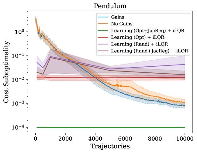
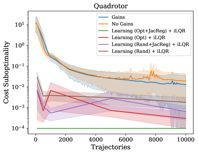
Though we find that our method outperforms deep-learning baselines (excluding OPT+JacReg) on the simpler inverted pendulum environment, the learning+$\mathtt{iLQR}$ approaches fare better on the quadrotor. We suspect that this is attributable to data-reuse, as Algorithm 1 estimates an entirely new model of system dynamics at each iteration. We believe that finding a way to combine the advantages of directly estimating linearized dynamics (observed in Algorithm 1, as well as OPT+JacReg) with the advantages of data-reuse.

Part I Analysis

Appendix A Formal Analysis

A.1 Organization of the Appendix

First, we begin with an outline of Appendix A:

• Section A.2 reviews essential notation.

• Section A.3 gives a restatement of our main result, Theorem 1, as Theorem 2.

The rest of Appendix A carries out the proof of Theorem 2. Speficially,

• Section A.4 defines numerous problem parameters on which our arguments depend.

• Section A.5 proves Corollary A.1, a precise statement of Proposition 4.2 in the main text. It does so via an intermediate result, Proposition A.4, which bounds the $\mathcal{L}_{\infty}$ difference between the continuous-time gradient, and the imagine of the discrete-time gradient under the continuous-time inclusion map $\mathsf{ct}(\cdot)$.

• Section A.6 states key results based on Taylor expansions of dynamics around their linearizations, and norms of various derivative-like quantities.

• Section A.7 contains the main statements of the various estimation guarantees, notably, the recovery of nominal trajectories, Markov operators, discretized gradients, and linearized transition matrices $({\color[rgb]{.1,0,.5}\mathtt{A}}^{\pi}_{\mathrm{ol},k},{\color[rgb]{.1,0,.5}\mathtt{B}}^{\pi}_{\mathrm{ol},k})$.

• Section A.8 leverages the previous section to demonstrate (a) a certain descent condition holds for each gradient step and (b) that sufficiently accurate estimates of transition matrices lead to the synthesis of gains for which the corresponding policies have bounded stability moduli.

• Finally, Section A.9 concludes the proof, as well as states a more granular guarantee in terms of specific problem parameters and not general $\mathcal{O}_{\star}(\cdot)$ notation.

The rest of Part I of the Appendix provides the proofs of constituent results. Specifically,

• Appendix B presents various discussion of main results, as well as gesturing to extensions. Specifcally, Section B.1 describes the exponential gap between $\mathtt{FOS}$s of $\mathcal{J}_{T}$ and $\mathtt{JSP}$s, and Section B.2 explains the consequences of combining our result with Westenbroek et al. (2021). We discuss how to implement a projection step to ensure Definition 4.7 in Section B.3. Finally, we discuss extensions to an oracle with process noise in Section B.4.

• Appendix C presents various computations of Jacobian linearizations, establishing that they do accurately capture first-order expansions.

• Appendix D proves all the Taylor-expansion like results listed in Section A.6.

• Appendix E proves all the estimation-error bounds in Section A.7.

• Appendix F provides a general certainty-equivalence and Lyapunov stability perturbation results for time-varying, discrete-time linear systems, in the regime that naturally arises when the state matrices are derived from discretizations of continuous-time dynamics.

• Appendix G instantiates the bounds in Appendix F to show that the gains synthesized by Algorithm 2 do indeed lead to policies with bounded stability modulus.

• Appendix H contains the proofs of optimization-related results: the proof of the descent lemma (Lemma A.13 (in Section H.1) and the proof of the conversion between stationary points and $\mathtt{JSP}$s, Proposition 4.1 (in Section H.2)

• Finally, Appendix I contains various time-discretization arguments, and in particular establishes the aforementiond Proposition A.4 from Section A.5.

A.2 Notation Review

In this section, we review our basic notation.

Dynamics.

Recall the nominal system dynamics are given by

$$\smash{\tfrac{\mathrm{d}}{\mathrm{d}t}}\mathbf{x}(t\mid\mathbf{u})=f_{\mathrm{dyn}}(\mathbf{x}(t\mid\mathbf{u}),\mathbf{u}(t)),~{}~{}\mathbf{x}(0\mid\mathbf{u})=\xi_{\mathrm{init}}.$$

We recall the definition of various stabilized dynamics.

See 2.1

See 4.4

Linearizations.

Next, we recall the definition of the various linearizations. See 4.2 See 4.6 We also recall the definition of stationary policies and $\mathtt{JSP}$s. See 2.2 See 2.4

Problem Constants.

We recall the dynamics-constants $\kappa_{f},L_{f},M_{f}$ defined in Assumption 4.1, $\kappa_{\mathrm{cost}},L_{\mathrm{cost}},M_{\mathrm{cost}}$ in Assumption 4.2, the strong-convexity parameter $\alpha$ in Assumption 2.1, the controllability parameters $t_{\mathrm{ctrl}},\nu_{\mathrm{ctrl}}$ from Assumption 4.4, with $k_{\mathrm{ctrl}}:=t_{\mathrm{ctrl}}/\uptau$, and the Riccati parameter $\mu_{\mathrm{ric}}$ from Assumption 4.3. Finally, we recall the feasibility radius from Condition 4.1. We also recall See 4.1

Gradient and Cost Shorthands.

Notably, we bound out the following shorthand for gradients and costs:

$$\nabla\mkern-2.5mu\mathcal{J}_{T}(\pi):=\nabla\mkern-2.5mu_{\mathbf{u}}\mathcal{J}_{T}^{\pi}(\mathbf{u})\big{|}_{\mathbf{u}=\mathbf{u}^{\pi}},\quad\nabla\mkern-2.5mu\mathcal{J}_{T}^{\mathrm{disc}}(\pi):=\nabla\mkern-2.5mu_{\vec{{\color[rgb]{.1,0,.5}\mathtt{u}}}}\mathcal{J}_{T}^{\pi,\mathrm{disc}}(\vec{{\color[rgb]{.1,0,.5}\mathtt{u}}})\big{|}_{\vec{{\color[rgb]{.1,0,.5}\mathtt{u}}}={\color[rgb]{.1,0,.5}\mathtt{u}}_{1:K}^{\pi}},\quad\mathcal{J}_{T}^{\mathrm{disc}}(\pi):=\mathcal{J}_{T}^{\pi,\mathrm{disc}}({\color[rgb]{.1,0,.5}\mathtt{u}}_{1:K}^{\pi}).$$ (A.1)

A.3 Full Statement of Main Result

The following is a slightly more general statement of Theorem 1, which implies Theorem 1 for appropriate choice of $\eta\leftarrow\frac{1}{c_{1}}\min\left\{\frac{1}{\sqrt{T}},1\right\}$, $\sigma_{w}\leftarrow(\sigma_{\mathrm{orac}}^{2}\iota(\delta)/N)^{\frac{1}{4}}$, and with the simplifications $\uptau\leq 1\leq T$.

Theorem 2.

Fix $\delta\in(0,1)$, define $\iota(\delta):=\log\frac{24T^{2}n_{\mathrm{iter}}\max\{d_{\mathsf{x}},d_{\mathsf{u}}\}}{\uptau^{2}\delta}$ and $\mathrm{Err}_{0}(\delta):=\sqrt{\iota(\delta)/N}$, where $N$ is the sample size, and suppose we select $\sigma_{w}=c(\sigma_{\mathrm{orac}}^{2}\iota(\delta)/N)^{\frac{1}{4}}$ for any $c\in[\frac{1}{\mathcal{O}_{\star}(1)},\mathcal{O}_{\star}(1)]$. Then, there exists constants $c_{1},c_{2},\dots,c_{5}=\mathcal{O}_{\star}(1)$ depending on $c$ such that the following holds. Suppose that

$$\eta\leq\frac{1}{c_{1}}\min\left\{\frac{1}{\sqrt{T}},1\right\},\quad\uptau\leq\frac{1}{c_{2}}\quad N\geq c_{3}\iota(\delta)\max\left\{1,\frac{T^{2}}{\uptau^{2}},\frac{1}{\uptau^{4}},T,\sigma_{\mathrm{orac}}^{2}\frac{T^{4}}{\uptau^{2}},\frac{\sigma_{\mathrm{orac}}^{2}}{\uptau^{8}}\right\}.$$ (A.2)

Then, with probability $1-\delta$, if Condition 4.1 and all listed Assumptions hold,

• For all $n\in[n_{\mathrm{iter}}]$, and $\pi^{\prime}\in\{\pi^{(n)},\tilde{\pi}^{(n)}\}$, $\mu_{\pi^{\prime},\star}\leq 8\mu_{\mathrm{ric}}$ and $L_{\pi^{\prime}}\leq 6\max\{1,L_{f}\}\mu_{\mathrm{ric}}$.

• For $\pi=\pi^{(n_{\mathrm{out}})}$, $\pi$ is $\epsilon$-stationary where

  $$\epsilon^{2}=c_{4}T\left(\uptau^{2}+\frac{1}{\eta}\left(\frac{1}{n_{\mathrm{iter}}}+\left(\eta T^{2}+\frac{T^{2}}{\uptau^{2}}\right)\left(\frac{\iota(\delta)^{2}}{N}+\sigma_{\mathrm{orac}}\sqrt{\frac{\iota(\delta)}{N}}\right)+\sigma_{\mathrm{orac}}^{2}\frac{\iota(\delta)^{2}}{N}\right)\right).$$

• For $\pi=\pi^{(n_{\mathrm{out}})}$, $\mathbf{u}^{\pi}$ is an $\epsilon^{\prime}$-$\mathtt{JSP}$, where $\epsilon^{\prime}=c_{5}\frac{\epsilon^{2}}{\alpha}$.

A.4 Problem Parameters

In this section, we provide all definitions of various problem paramaters. The notation is extensive, but we maintain the following conventions:

1. $\mu_{(\cdot)}$ refers to upper bounds on Lyapunov operators, $\kappa_{(\cdot)}$ to upper bounds on zero-order terms (e.g. $\|f_{\mathrm{dyn}}(x,u)\|$) or magnitudes of transition operators, $M_{(\cdot)}$ to bounds on second-order derivatives, $L_{(\cdot)}$ to bounds on first-order derivatives, $B_{(\cdot)}$ to upper bounds on radii, $\uptau_{(\cdot)}$ to step sizes, $\mathrm{Err}_{(\cdot)}$ to error terms.

2. $q\in\{1,2,\infty\}$ corresponds to $\ell_{q}$ norms

3. Subscripts $\mathrm{tay}$ denote relevance to Taylor expansions of the dynamics.

4. Terms with have a subscript $\pi$ hide dependence on $L_{\pi}$, $\mu_{\pi,\star}$ and ${\kappa}_{q}$ for $q\in\{1,2,\infty\}$

Remark A.1 (Reminder on Asymptotic Notation).

We let $\mathcal{O}_{\star}(x)$ denote a term which suppresses polynomial dependence on all the constants in Assumptions 4.1 and 4.2, as well as $\mu_{\mathrm{ric}}$ in Assumption 4.3, and $\nu_{\mathrm{ctrl}}$, $t_{0}\geq t_{\mathrm{ctrl}}$ and $e^{L_{f}t_{0}}\geq e^{L_{f}t_{\mathrm{ctrl}}}$, where $t_{0}=\uptau k_{0}$, and $\nu_{\mathrm{ctrl}},t_{\mathrm{ctrl}}$ are given in Assumption 4.4. We let $\mathcal{O}_{\pi}(x)$ suppress all of these constants, as well as polynomials in $L_{\pi}$ and $\mu_{\pi,\star}$.

A.4.1 Stability Constants

We begin by recalling the primary constants controlling the stability of a policy $\pi$. See 4.7 It is more convenient to prove bounds in terms of the following three quantity, which are defined in terms of the magnitudes of the closed-loop transition operators.

Definition A.1 (Norms of $\pi$).

We define the constants $\kappa_{\pi,\infty}:=\max_{1\leq j\leq k\leq K+1}\|{\color[rgb]{.1,0,.5}\mathtt{\Phi}}^{\pi}_{\mathrm{cl},k,j}\|$, and

$$\kappa_{\pi,1} :=\max_{k\in[K+1]}\uptau\left(\sum_{j=1}^{k}\|{\color[rgb]{.1,0,.5}\mathtt{\Phi}}^{\pi}_{\mathrm{cl},k,j}\|\vee\sum_{j=k}^{K+1}\|{\color[rgb]{.1,0,.5}\mathtt{\Phi}}^{\pi}_{\mathrm{cl},j,k}\|\right)$$

$$\kappa_{\pi,2}^{2} :=\max_{k\in[K+1]}\uptau\left(\sum_{j=1}^{k}\|{\color[rgb]{.1,0,.5}\mathtt{\Phi}}^{\pi}_{\mathrm{cl},k,j}\|^{2}\vee\sum_{j=k}^{K+1}\|{\color[rgb]{.1,0,.5}\mathtt{\Phi}}^{\pi}_{\mathrm{cl},j,k}\|^{2}\right)$$

We also define the following upper bounds on these quantities:

$$\kappa_{\infty}(\mu,L) :=\sqrt{\max\{1,6L_{f}L\}\mu}\exp(t_{0}L_{f})$$

$$\kappa_{2}(\mu,L) :=\max\{1,6L_{f}L\}\mu\left(t_{0}\exp(2t_{0}L_{f})+\mu\right)$$

$$\kappa_{1}(\mu,L) :=\sqrt{\max\{1,6L_{f}L\}\mu}\left(t_{0}\exp(t_{0}L_{f})+2\mu\right)$$

The following lemma is proven in Section G.4, and shows that shows that each of the above terms is $\mathcal{O}_{\pi}(1)$.

Lemma A.1.

Let $\pi$ be any policy. Recall $t_{0}=\uptau k_{0}$ Then, as long as $\uptau\leq 1/6L_{f}L_{\pi}$,

$$\mu_{\pi,q}\leq\mu_{q}(\mu_{\pi,\star},L_{\pi})=\mathcal{O}_{\pi}(1).$$

A.4.2 Discretization Step Magnitudes

Next, we introduce various maximal discretization step sizes for which our discrete-time dynamics are sufficiently faithful to the continuous ones. The first is a general condition for the dynamics to be “close”, the second is useful for closeness of solutions of Ricatti equations, the third for the discrete-time dynamics to admit useful Taylor expansions, and the fourth for discrete-time controllability. We note that the first two do not depend on $\pi$, while the second two do.

Definition A.2 (Discretization Sizes).

We define

$$\uptau_{\mathrm{dyn}} :=\frac{1}{4L_{f}}$$

$$\uptau_{\mathrm{ric}} :=\frac{1}{4\mu_{\mathrm{ric}}^{2}\left(3M_{f}\kappa_{f}\mu_{\mathrm{ric}}L_{f}+13L_{f}^{2}(1+L_{f}\mu_{\mathrm{ric}})^{2}\right)}$$

$$\uptau_{\mathrm{tay},\pi} :=\min\left\{\frac{1}{16L_{f}L_{\pi}},\frac{1}{8\kappa_{f}}\right\}\leq\uptau_{\mathrm{dyn}}.$$

$$\uptau_{\mathrm{ctrl},\pi} :=\frac{\nu_{\mathrm{ctrl}}}{8L_{\pi}^{2}K_{\mathrm{\pi}}^{2}\gamma_{\mathrm{ctr}}^{3}\exp(2\gamma_{\mathrm{ctr}})\left(\kappa_{f}M_{f}+2L_{f}^{2}\right)},\quad\gamma_{\mathrm{ctr}}:=\max\{1,L_{f}t_{\mathrm{ctrl}}\}$$

We note that $\uptau_{\mathrm{dyn}},\uptau_{\mathrm{ric}}=1/\mathcal{O}_{\star}(1)$ and $\uptau_{\mathrm{tay},\pi},\uptau_{\mathrm{ctrl},\pi}=1/\mathcal{O}_{\pi}(1)$.

A.4.3 Taylor Expansion Constants.

We now define the relevant constants in terms of which we bound our taylor expansions.

Definition A.3 (Taylor Expansion Constants, Policy Dependent).

We define $L_{\mathrm{tay},\infty,\pi}=2L_{f}\kappa_{\pi,1}$, $L_{\mathrm{tay},2,\pi}:=2L_{f}\kappa_{\pi,2}$, and

$$M_{\mathrm{tay},2,\pi} :=8M_{f}(\kappa_{\pi,\infty}+10L_{\pi}^{2}L_{f}^{2}\kappa_{\pi,2}^{2}\kappa_{\pi,1})$$

$$M_{\mathrm{tay},\inf,\pi} :=8M_{f}(\kappa_{\pi,1}+10L_{\pi}^{2}L_{f}^{2}\kappa_{\pi,1}^{3})$$

$$B_{\mathrm{tay},2,\pi} =\min\left\{\frac{1}{\sqrt{40M_{f}L_{\pi}^{2}\kappa_{\pi,1}M_{\mathrm{tay},2,\pi}}},\frac{L_{f}\kappa_{\pi,2}}{2M_{\mathrm{tay},2,\pi}},\frac{R_{\mathrm{feas}}}{16L_{\pi}L_{f}\kappa_{\pi,2}}\right\}$$

$$B_{\mathrm{tay},\inf,\pi} =\min\left\{\frac{1}{40L_{\pi}^{2}\kappa_{\pi,1}M_{\mathrm{tay},\inf,\pi}},\frac{L_{f}\kappa_{\pi,1}}{2M_{\mathrm{tay},\inf,\pi}},\frac{R_{\mathrm{feas}}}{16L_{\pi}L_{f}\kappa_{\pi,1}}\right\}$$

We also define

$$M_{\mathcal{J},\mathrm{tay},\pi} :=2M_{\mathrm{cost}}L_{f}^{2}\kappa_{\pi,2}^{2}(1+3L_{\pi}^{2}T)M_{\mathrm{tay},2,\pi}+L_{\mathrm{cost}}(1+2L_{\pi}T)M_{\mathrm{tay},2,\pi}+2L_{\pi}L_{\mathrm{cost}},$$

$$B_{\mathrm{stab},\pi} :=\left(\max\{6,36L_{f}L_{\pi}\}\mu_{\pi,\star}\cdot 12TM_{f}L_{\pi}(1+L_{f}K_{\mathrm{\pi}})B_{\infty}\right)^{-1}$$

$$L_{\nabla\mkern-2.5mu,\pi,\infty} :=L_{\mathrm{cost}}(1+\frac{3L_{f}}{2}\kappa_{\pi,\infty}+3L_{\pi}\kappa_{\pi,1})$$

The following is a consequence of Lemma A.1.

Lemma A.2.

By Lemma A.1, $M_{\mathrm{tay},2,\pi},M_{\mathrm{tay},\inf,\pi},L_{\nabla\mkern-2.5mu,\pi,\infty},L_{\mathrm{tay},q,\pi}=\mathcal{O}_{\pi}(1)$, $B_{\mathrm{tay},2,\pi},B_{\mathrm{tay},\inf,\pi}=1/\mathcal{O}_{\pi}(1)$, $M_{\mathcal{J},\mathrm{tay},\pi}=T\cdot\mathcal{O}_{\pi}(1)$, and $B_{\mathrm{stab},\pi}=\frac{1}{T}\cdot\mathcal{O}_{\pi}(1)$.

The first group of four constants arises in Taylor expansions of the dynamics, the fith in a Taylor expansion of the cost functional, and the sixth in controlling the stability of policies under changes to the input, and the last upper bounds the norm of the gradient.

A.4.4 Estimation Error Terms.

Finally, we define the following error terms which arise in the errors of the extimated nominal trajectories, Markov operators, and gradients. Note that the first term has no dependence on $\pi$, while the latter two do.

Definition A.4 (Error Terms).

Define $\iota(\delta):=\log\frac{24T^{2}n_{\mathrm{iter}}\max\{d_{\mathsf{x}},d_{\mathsf{u}}\}}{\uptau^{2}\delta}=\log\frac{24K^{2}n_{\mathrm{iter}}d_{\star}}{\delta}$, where $d_{\star}:=\max\{d_{\mathsf{x}},d_{\mathsf{u}}\}$. Further, define

$$\mathrm{Err}_{\hat{x}}(\delta) :=\sigma_{\mathrm{orac}}\sqrt{2\frac{d_{\star}\iota(\delta)}{N}}$$

$$\mathrm{Err}_{\Psi,\pi}(\delta) :=\sqrt{\frac{\iota(\delta)}{N}}\left(\frac{2\sigma_{\mathrm{orac}}}{\sigma_{w}}d_{\star}^{3/2}+8L_{\mathrm{tay},\infty,\pi}d_{\star}\right)+4\sigma_{w}M_{\mathrm{tay},2,\pi}d_{\star}^{3/2}=\mathcal{O}_{\pi}(\sqrt{\frac{\iota(\delta)}{N}}(1+\frac{\sigma_{\mathrm{orac}}}{\sigma_{w}}+\sigma_{w})$$

$$\mathrm{Err}_{\nabla\mkern-2.5mu,\pi}(\delta) :=\left(L_{\mathrm{cost}}\mathrm{Err}_{\Psi,\pi}(\delta)+(1+\kappa_{\pi,\infty})M_{\mathrm{cost}}\mathrm{Err}_{\hat{x}}(\delta)\right)(1+2TL_{\pi}).$$

We note that, in view of Lemma A.1,

By Lemmas A.1 and A.2, we have

Lemma A.3.

Define $\mathrm{Err}_{0}(\delta)=\sqrt{\frac{\iota(\delta)}{N}}$. Then,

$$\mathrm{Err}_{\hat{x}}(\delta) =\sigma_{\mathrm{orac}}\sqrt{2d_{\star}}\mathrm{Err}_{0}(\delta)\leq\mathcal{O}_{\star}\left(\mathrm{Err}_{0}(\delta)\right)$$ (A.3)

$$\mathrm{Err}_{\Psi}(\delta) \leq\mathcal{O}_{\pi}\left(\mathrm{Err}_{0}(\delta)(1+\frac{\sigma_{\mathrm{orac}}}{\sigma_{w}})+\sigma_{w}\right)$$

$$\mathrm{Err}_{\nabla\mkern-2.5mu,\pi}(\delta) \leq\mathcal{O}_{\pi}\left(T\left(\mathrm{Err}_{0}(\delta)(1+\sigma_{\mathrm{orac}}+\frac{\sigma_{\mathrm{orac}}}{\sigma_{w}})+\sigma_{w}\right)\right).$$

If we further tune $\sigma_{w}=c\sqrt{\sigma_{\mathrm{orac}}\mathrm{Err}_{0}(\delta)}$ for any $c\in[1/\mathcal{O}_{\star}(1),\mathcal{O}_{\star}(1)]$, then

$$\mathrm{Err}_{\hat{x}}(\delta) \leq\mathcal{O}_{\star}\left(\sigma_{\mathrm{orac}}\mathrm{Err}_{0}(\delta)\right)$$ (A.4)

$$\mathrm{Err}_{\Psi}(\delta) \leq\mathcal{O}_{\pi}\left(\mathrm{Err}_{0}(\delta)+\sqrt{\sigma_{\mathrm{orac}}\mathrm{Err}_{0}(\delta)}\right)$$

$$\mathrm{Err}_{\nabla\mkern-2.5mu,\pi}(\delta) \leq\mathcal{O}_{\pi}\left(T\left(\mathrm{Err}_{0}(\delta)+\sqrt{\sigma_{\mathrm{orac}}\mathrm{Err}_{0}(\delta)}\right)\right).$$

A.5 Gradient Discretization

We begin by stating with the precise statement of Proposition 4.2, which relates norms of gradients of the discretized objective to that of the continuous-time one. We begin with the following proposition which bounds the difference between the continuous-time gradient, and a (normalized) embedding of the discrete-time gradient into continuous-time. We define the constant

$$\kappa_{\nabla\mkern-2.5mu}:=\left((1+L_{f})M_{\mathrm{cost}}(1+\kappa_{f})+L_{\mathrm{cost}}(3\kappa_{f}M_{f}+8L_{f}^{2}+L_{f})\right)=\mathcal{O}_{\star}(\cdot){1}$$ (A.5)

Proposition A.4 (Discretization of the Gradient).

Let $\pi$ be feasible, and let $\tilde{\nabla\mkern-2.5mu}\mathcal{J}_{T}(\pi)=\frac{1}{\uptau}\uptau(\nabla\mkern-2.5mu\mathcal{J}_{T}^{\mathrm{disc}}(\pi))$ is the continuous-time inclusion of the discrete-time gradient, normalized by $\uptau^{-1}$. Then,

$$\sup_{t\in[0,T)}\|\nabla\mkern-2.5mu\mathcal{J}_{T}(\pi)(t)-\tilde{\nabla}\mkern-2.5mu\mathcal{J}_{T}(\pi)(t)\|\leq\uptau e^{\uptau L_{f}}\max\{\kappa_{\pi,\infty},\kappa_{\pi,1},1\}L_{\pi}\kappa_{\nabla\mkern-2.5mu},$$

The above result is proven in Section I.3. By integrating, we see that $\|\nabla\mkern-2.5mu\mathcal{J}_{T}(\pi)-\tilde{\nabla}\mkern-2.5mu\mathcal{J}_{T}(\pi)\|_{\mathcal{L}_{2}(\mathcal{U})}\leq\sqrt{T}\uptau e^{\uptau L_{f}}\max\{\kappa_{\pi,\infty},\kappa_{\pi,1},1\}L_{\pi}\kappa_{\nabla\mkern-2.5mu}$, and thus the triangle inequality gives $\|\nabla\mkern-2.5mu\mathcal{J}_{T}(\pi)\|_{\mathcal{L}_{2}(\mathcal{U})}\leq\|\tilde{\nabla\mkern-2.5mu}\mathcal{J}_{T}(\pi)\|_{\mathcal{L}_{2}(\mathcal{U})}+\sqrt{T}\uptau e^{\uptau L_{f}}\max\{\kappa_{\pi,\infty},\kappa_{\pi,1},1\}L_{\pi}\kappa_{\nabla\mkern-2.5mu}$. We can see that for any $\vec{{\color[rgb]{.1,0,.5}\mathtt{u}}}={\color[rgb]{.1,0,.5}\mathtt{u}}_{1:K}\in\mathsf{U}$, $\|\vec{{\color[rgb]{.1,0,.5}\mathtt{u}}}\|_{\ell_{2}}^{2}=\sum_{k=1}^{K}\|{\color[rgb]{.1,0,.5}\mathtt{u}}_{k}\|^{2}=\frac{1}{\uptau}\int_{0}^{T}\|{\color[rgb]{.1,0,.5}\mathtt{u}}_{k(t)}\|^{2}=\frac{1}{\uptau}\|\mathsf{ct}(\vec{{\color[rgb]{.1,0,.5}\mathtt{u}}})\|_{\mathcal{L}_{2}(\mathcal{U})}^{2}$. Hence, in particular, $\|\nabla\mkern-2.5mu\mathcal{J}_{T}(\pi)\|_{\mathcal{L}_{2}(\mathcal{U})}\leq\frac{1}{\sqrt{\uptau}}\|\nabla\mkern-2.5mu\mathcal{J}_{T}^{\mathrm{disc}}(\pi)\|_{\ell_{2}}+\sqrt{T}\uptau e^{\uptau L_{f}}\max\{\kappa_{\pi,\infty},\kappa_{\pi,1},1\}L_{\pi}\kappa_{\nabla\mkern-2.5mu}$. From this, and from using Lemma A.1 to bound $\kappa_{\pi,\infty},\kappa_{\pi,1}=\mathcal{O}_{\pi}(1)$, we obtain the following corollary, which is a precise statement of Proposition 4.2.

Corollary A.1.

Suppose $\pi$ is feasible. Then, recalling $\kappa_{\nabla\mkern-2.5mu}$ from Eq. A.5,

$$\|\nabla\mkern-2.5mu\mathcal{J}_{T}(\pi)\|_{\mathcal{L}_{2}(\mathcal{U})}\leq\frac{1}{\sqrt{\uptau}}\|\nabla\mkern-2.5mu\mathcal{J}_{T}^{\mathrm{disc}}(\pi)\|_{\ell_{2}}+\sqrt{T}\uptau e^{\uptau L_{f}}\max\{\kappa_{\pi,\infty},\kappa_{\pi,1},1\}L_{\pi}\kappa_{\nabla\mkern-2.5mu}.$$

In particular, for $\uptau\leq 1/4L_{f}$,

$$\|\nabla\mkern-2.5mu\mathcal{J}_{T}(\pi)\|_{\mathcal{L}_{2}(\mathcal{U})}\leq\frac{1}{\sqrt{\uptau}}\|\nabla\mkern-2.5mu\mathcal{J}_{T}^{\mathrm{disc}}(\pi)\|_{\ell_{2}}+\sqrt{T}\uptau\cdot\underbrace{2\max\{\kappa_{\pi,\infty},\kappa_{\pi,1},1\}L_{\pi}\kappa_{\nabla\mkern-2.5mu}}_{=\mathcal{O}_{\pi}(1)}.$$

A.6 Main Taylor Expansion Results

We now state various bounds on Taylor-expansion like terms. All the following results are proven in Appendix D. The first is a Taylor expansion of the dynamics (proof in Section D.1).

Proposition A.5.

Let $\pi$ be feasible, $\uptau\leq\uptau_{\mathrm{tay},\pi}$ Fix a ${\color[rgb]{.1,0,.5}\mathtt{u}}_{1:K}\in\bm{\mathsf{U}}$, and define the perturbation $\updelta{{\color[rgb]{.1,0,.5}\mathtt{u}}}_{1:K}:={\color[rgb]{.1,0,.5}\mathtt{u}}_{1:K}-{\color[rgb]{.1,0,.5}\mathtt{u}}_{1:K}^{\pi}$, and define

$$B_{2}:=\sqrt{\uptau}\|\updelta{{\color[rgb]{.1,0,.5}\mathtt{u}}}_{1:K}\|_{\ell_{2}},B_{\infty}:=\max_{k}\|\updelta{{\color[rgb]{.1,0,.5}\mathtt{u}}}_{k}\|.$$

Then, if $B_{\infty}\leq R_{\mathrm{feas}}/8$, and if for either $q\in\{2,\infty\}$, it holds that $B_{q}\leq B_{\mathrm{tay},q,\pi}$, then

• The following bounds hold for all $k\in[K+1]$

  $$\|\tilde{{\color[rgb]{.1,0,.5}\mathtt{x}}}^{\pi}_{k}\,({\color[rgb]{.1,0,.5}\mathtt{u}}_{1:K}])-{\color[rgb]{.1,0,.5}\mathtt{x}}_{k}^{\pi}-\sum_{j=1}^{k-1}{\color[rgb]{.1,0,.5}\mathtt{\Psi}}^{\pi}_{\mathrm{cl},k,j}\updelta{{\color[rgb]{.1,0,.5}\mathtt{u}}}_{j}\|\leq M_{\mathrm{tay},q,\pi}B_{q}^{2},\quad\|\tilde{{\color[rgb]{.1,0,.5}\mathtt{x}}}^{\pi}_{k}\,({\color[rgb]{.1,0,.5}\mathtt{u}}_{1:K})-{\color[rgb]{.1,0,.5}\mathtt{x}}_{k}^{\pi}\|\leq L_{\mathrm{tay},q,\pi}B_{q},$$

• Moreover, for all $k\in[K+1]$ and $t\in[0,T]$,

  $$\max\{\|\tilde{{\color[rgb]{.1,0,.5}\mathtt{x}}}^{\pi}_{k}\,({\color[rgb]{.1,0,.5}\mathtt{u}}_{1:K})\|,\|\tilde{{\color[rgb]{.1,0,.5}\mathtt{u}}}^{\pi}_{k}\,({\color[rgb]{.1,0,.5}\mathtt{u}}_{1:K}])\}\leq\frac{3R_{\mathrm{feas}}}{4},and\|\tilde{\mathbf{x}}^{\pi}(t\mid{\color[rgb]{.1,0,.5}\mathtt{u}}_{1:K})\|\leq R_{\mathrm{feas}}.$$

Next, we provide a Taylor expansion of the discrete-time cost functional (proof in Section D.2).

Lemma A.6.

Consider the setting of Proposition A.5, and suppose $B_{\infty}\leq R_{\mathrm{feas}}/8$ and $B_{2}\leq B_{\mathrm{tay},2,\pi}$. Then,

$$\|\mathcal{J}_{T}^{\pi,\mathrm{disc}}(\updelta{{\color[rgb]{.1,0,.5}\mathtt{u}}}_{1:K}+{\color[rgb]{.1,0,.5}\mathtt{u}}_{1:K}^{\pi})-\mathcal{J}_{T}^{\pi,\mathrm{disc}}({\color[rgb]{.1,0,.5}\mathtt{u}}_{1:K}^{\pi})-\langle\updelta{{\color[rgb]{.1,0,.5}\mathtt{u}}}_{k},\nabla\mkern-2.5mu\mathcal{J}_{T}^{\pi,\mathrm{disc}}({\color[rgb]{.1,0,.5}\mathtt{u}}_{1:K}^{\pi})\rangle\|\leq M_{\mathcal{J},\mathrm{tay},\pi}B_{2}^{2}.$$

Next, we show sufficiently small perturbations of the nomimal input preserve stability of the dynamics (proof in Section D.3).

Lemma A.7.

Again consider the setting of Proposition A.5, and suppose $B_{\infty}\leq\min\{R_{\mathrm{feas}}/8,B_{\mathrm{tay},\inf,\pi},B_{\mathrm{stab},\pi}\}$. Then,

$$\mu_{\pi^{\prime},\star}\leq(1+B_{\infty}/B_{\mathrm{stab},\pi})\mu_{\pi,\star}\leq 2\mu_{\pi,\star},\quad L_{\pi^{\prime}}=L_{\pi}.$$

Lastly, we bound the norm of the discretized gradient (Section D.4).

Lemma A.8.

Let $\pi$ be feasible, and let $\uptau\leq\uptau_{\mathrm{dyn}}$. Then

$$\max_{k\in[K]}\|(\nabla\mkern-2.5mu\mathcal{J}_{T}^{\mathrm{disc}}(\pi))_{k}\|\leq\uptau L_{\nabla\mkern-2.5mu,\pi,\infty}$$

A.7 Estimation Errors

In this section, we bound the various estimation errors. All the proofs are given in Appendix E. We begin with a simple condition we need for estimation of Markov parameters to go through.

Definition A.5.

We say $\pi$ is estimation-friendly if $\pi$ is feasible, and if

$$\sigma_{\mathrm{orac}}\sqrt{\frac{\iota(\delta)}{2NL_{\pi}}}\leq\sigma_{w}\leq\frac{B_{\mathrm{tay},\inf,\pi}}{2\sqrt{d_{\star}}},\quad\uptau\leq\uptau_{\mathrm{tay},\pi}$$

Our first result is recovery of the nominal trajectory and Markov operators. Recovery of the nominal trajectory follows from Gaussian concentration, and recovery of the Markov operator for the Matrix Hoeffding inequality (Tropp (2012, Theorem 1.4)) combined with the Taylor expansion of the dynamics due to Proposition A.5. The following is proven in Section E.1. To state the bound, we recall the estimation error terms in Definition A.4.

Proposition A.9.

Fix $\delta\in(0,1)$ and suppose that $N$ is large enough that $\pi$ is estimation friendly. Then, for any estimation-friendly $\textsc{EstMarkov}(\pi;N,\sigma_{w})$ (Algorithm 2) returns estimates with such that, with probability $1-\delta/2n_{\mathrm{iter}}$.

$$\max_{1\leq j<k\leq K+1}\left\|{\color[rgb]{.1,0,.5}\mathtt{\Psi}}^{\pi}_{\mathrm{cl},k,j}-\hat{{\color[rgb]{.1,0,.5}\mathtt{\Psi}}}_{k,j}\right\|_{\mathrm{op}}\leq\mathrm{Err}_{\Psi,\pi}(\delta)\quad\max_{k\in[K+1]}\|\hat{{\color[rgb]{.1,0,.5}\mathtt{x}}}_{k}-{\color[rgb]{.1,0,.5}\mathtt{x}}_{k}^{\pi}\|\leq\mathrm{Err}_{\hat{x}}(\delta)$$ (A.6)

Let $\Pi_{\mathrm{alg}}:=\{\pi^{(n)},\tilde{\pi}^{(n)}:n\in[n_{\mathrm{iter}}]\}$ denote the set of policies constructed by the algorithm, and note that EstMarkov is called once for each policy in $\Pi_{\mathrm{alg}}$. We define the good estimation event as

$$\mathcal{E}_{\mathrm{est}}(\delta) :=\bigcap_{n=1}^{\infty}(\mathcal{E}_{n}(\delta)\cap\tilde{}\mathcal{E}_{n}(\delta)),\quad$$ (A.7)

$$\mathcal{E}_{n}(\delta) :=\{\text{\lx@cref{creftypecap~refnum}{eq:good_event} holds for $\pi=\pi^{(n)}$ if $\pi^{(n)}$ is estimation friendly}\}$$ (A.8)

$$\tilde{}\mathcal{E}_{n}(\delta) :=\{\text{\lx@cref{creftypecap~refnum}{eq:good_event}holds for $\tilde{\pi}=\pi^{(n)}$ if $\tilde{\pi}^{(n)}$ is estimation-friendly}\}$$ (A.9)

By Proposition A.9 and a union bound implies

$$\operatorname{\mathbb{P}}[\mathcal{E}_{\mathrm{est}}(\delta)]\geq 1-\delta.$$

We now show that on the good estimation event, the error of the gradient is bounded. The proof is Section E.2.

Lemma A.10 (Gradient Error).

On the event $\mathcal{E}_{\mathrm{est}}(\delta)$, it holds that that if $\pi^{(n)}$ is estimation-friendly, then Algorithm 1(4) produces

$$\max_{k}\|\hat{{\color[rgb]{.1,0,.5}\mathtt{\nabla\mkern-2.5mu}}}_{k}^{\,(n)}-(\nabla\mkern-2.5mu\mathcal{J}_{T}^{\mathrm{disc}}(\pi^{(n)}))_{k}\|\leq\mathrm{Err}_{\nabla\mkern-2.5mu,\pi^{(n)}}(\delta).$$

We also bound the error in the recovery of the system paramters used for synthesizing the stabilizing gains. Recovery of said parameters requires first establishing controllability of the discrete-time Markov operator. We prove the following in Section E.3:

Proposition A.11.

Define $\gamma_{\mathrm{ctr}}:=\max\{1,L_{f}t_{\mathrm{ctrl}}\}$, and suppose that $\uptau\leq\min\{\uptau_{\mathrm{ctrl},\pi},\uptau_{\mathrm{dyn}}\}$. Then, for $k\geq k_{\mathrm{ctrl}}+1$, it holds that

$$\lambda_{\min}\left(\sum_{j=k-k_{\mathrm{ctrl}}}^{k-1}{\color[rgb]{.1,0,.5}\mathtt{\Psi}}^{\pi}_{\mathrm{cl},k,j}({\color[rgb]{.1,0,.5}\mathtt{\Psi}}^{\pi}_{\mathrm{cl},k,j})^{\top}\right)\succeq\uptau\cdot\frac{\nu_{\mathrm{ctrl}}}{8L_{\pi}^{2}\gamma_{\mathrm{ctr}}^{2}\exp(2\gamma_{\mathrm{ctr}})}$$

With this result, Section E.4 upper bounds the estimation error for the discrete-time system matrices.

Proposition A.12.

Suppose $\mathcal{E}_{\mathrm{est}}(\delta)$ holds, fix $n\in n_{\mathrm{iter}}$, and let $\pi=\tilde{\pi}^{(n)}$. Then, suppose that $\uptau\leq\min\{\uptau_{\mathrm{ctrl},\pi},\uptau_{\mathrm{dyn}}\}$, $k_{0}\geq k_{\mathrm{ctrl}}+2$, and

$$\mathrm{Err}_{\Psi}(\delta)\leq\uptau\frac{\sqrt{\nu_{\mathrm{ctrl}}/t_{\mathrm{ctrl}}}}{2\sqrt{2}L_{\pi}\gamma_{\mathrm{ctr}}\exp(\gamma_{\mathrm{ctr}})},$$ (A.10)

Then, on $\mathcal{E}_{\mathrm{est}}(\delta)$, if $\pi$ is estimation-friendly, the estimates from the call of $\textsc{EstGains}(\pi;N,\sigma)$ satisfy

$$\|\hat{{\color[rgb]{.1,0,.5}\mathtt{B}}}_{k}-{\color[rgb]{.1,0,.5}\mathtt{B}}^{\pi}_{\mathrm{ol},k}\|\vee\|\hat{{\color[rgb]{.1,0,.5}\mathtt{A}}}_{k}-{\color[rgb]{.1,0,.5}\mathtt{A}}^{\pi}_{\mathrm{ol},k}\|\leq\frac{\mathrm{Err}_{\Psi,\pi}(\delta)}{\uptau}\cdot t_{0}\kappa_{\pi,\infty}L_{\pi}^{2}\frac{192\gamma_{\mathrm{ctr}}^{3}\exp(2\gamma_{\mathrm{ctr}})}{\nu_{\mathrm{ctrl}}}.$$

A.8 Descent and Stabilization

In this section, we leverage the estimation results in the previous section to demonstrate the two key features of the algorithm: descent on the discrete-time objective, and stability after the synthesized gains. We begin with a standard first-order descent lemma, whose proof is given in Section H.1. This lemma also ensures, by invoking Lemma A.1, that the step size is sufficently small to control the stability of $\tilde{\pi}^{(n)}$, which uses the same gains as $\pi^{(n)}$ but has a slightly perturbed control input.

Lemma A.13 (Descent Lemma).

Suppose $\pi=\pi^{(n)}$ is estimation friendly, let $M\geq M_{\mathcal{J},\mathrm{tay},\pi}$, and suppose

$$\eta \leq\frac{1}{4M},\quad(\eta(L_{\nabla\mkern-2.5mu,\pi,\infty}+\frac{1}{\uptau}\mathrm{Err}_{\nabla\mkern-2.5mu,\pi^{(n)}}(\delta))+\mathrm{Err}_{\hat{x}}(\delta))\leq\min\left\{\frac{R_{\mathrm{feas}}}{8},B_{\mathrm{stab},\pi},B_{\mathrm{tay},\inf,\pi},\frac{B_{\mathrm{tay},2,\pi}}{\sqrt{T}}\right\}.$$

Then, on event $\mathcal{E}_{\mathrm{est}}(\delta)$, it holds (again setting $\pi\leftarrow\pi^{(n)}$ on the right-hand side)

$$\mathcal{J}_{T}^{\mathrm{disc}}(\tilde{\pi}^{(n)})-\mathcal{J}_{T}^{\mathrm{disc}}(\pi^{(n)}) \leq-\frac{\eta}{2\uptau}\|\hat{{\color[rgb]{.1,0,.5}\mathtt{\nabla\mkern-2.5mu}}}_{1:K}^{\,(n)}\|_{\ell_{2}}^{2}+T\left(\frac{\mathrm{Err}_{\nabla\mkern-2.5mu,\pi}(\delta)^{2}}{4\uptau^{2}M}+\mathrm{Err}_{\hat{x}}(\delta)L_{\nabla\mkern-2.5mu,\pi,\infty}+M\mathrm{Err}_{\hat{x}}(\delta)^{2}\right).$$

and that

$$L_{\tilde{\pi}^{(n)}}=L_{\pi^{(n)}},\quad\mu_{\tilde{\pi}^{(n)},\star}\leq 2\mu_{\pi^{(n)},\star}.$$

The next step is to establish a stability guarantee for the certainty-equivalent gains synthesized. We begin with a generic guarantee, whose proof is given in Appendix G.

Proposition A.14 (Certainty Equivalence Bound).

Let $\hat{{\color[rgb]{.1,0,.5}\mathtt{A}}}^{\pi}_{k}$ and $\hat{{\color[rgb]{.1,0,.5}\mathtt{B}}}^{\pi}_{k}$ be estimates of ${\color[rgb]{.1,0,.5}\mathtt{A}}^{\pi}_{\mathrm{ol},k}$ and ${\color[rgb]{.1,0,.5}\mathtt{B}}^{\pi}_{\mathrm{ol},k}$, and let $\hat{{\color[rgb]{.1,0,.5}\mathtt{K}}}_{k}$ denote the corresponding certainty equivalence controller synthesized by Algorithm 3(9 and 12). Suppose that $\uptau\leq\min\{\uptau_{\mathrm{ric}},\uptau_{\mathrm{dyn}}\}$ and

$$\max_{k\in[k_{0}:K]}\|\hat{{\color[rgb]{.1,0,.5}\mathtt{A}}}^{\pi}_{k}-{\color[rgb]{.1,0,.5}\mathtt{A}}^{\pi}_{\mathrm{ol},k}\|_{\mathrm{op}}\vee\|\hat{{\color[rgb]{.1,0,.5}\mathtt{B}}}^{\pi}_{k}-{\color[rgb]{.1,0,.5}\mathtt{B}}^{\pi}_{\mathrm{ol},k}\|_{\mathrm{op}}\leq\uptau(2^{17}\mu_{\mathrm{ric}}^{4}\max\{1,L_{f}^{3}\})^{-1}$$

Then, if $\pi^{\prime}=({\color[rgb]{.1,0,.5}\mathtt{u}}_{1:K}^{\pi},\hat{{\color[rgb]{.1,0,.5}\mathtt{K}}}_{1:K})$, we have

$$\mu_{\pi^{\prime},\star}\leq 4\mu_{\mathrm{ric}},\quad L_{\pi^{\prime}}\leq 6\max\{1,L_{f}\}\mu_{\mathrm{ric}}.$$

As a direct corollary of the above proposition and Proposition A.12, we obtain the following:

Lemma A.15.

Suppose $\mathcal{E}_{\mathrm{est}}(\delta)$ holds, fix $n\in n_{\mathrm{iter}}$, and let $\pi=\tilde{\pi}^{(n)}$. Then, suppose that $\uptau\leq\min\{\uptau_{\mathrm{ctrl},\pi},\uptau_{\mathrm{dyn}}\}$, $\pi$ is estimation-friendly, $k_{0}\geq k_{\mathrm{ctrl}}+2$, and

$$\mathrm{Err}_{\Psi,\pi}(\delta)\leq\uptau^{2}\left(2^{25}\mu_{\mathrm{ric}}^{4}\max\{1,L_{f}^{3}\}\cdot t_{0}\kappa_{\pi,\infty}L_{\pi}^{2}\frac{\gamma_{\mathrm{ctr}}^{3}\exp(2\gamma_{\mathrm{ctr}})}{\nu_{\mathrm{ctrl}}}\right)^{-1}$$ (A.11)

Then,

$$\mu_{\pi^{(n+1)},\star}\leq 4\mu_{\mathrm{ric}},\quad L_{\pi^{(n+1)}}\leq 6\max\{1,L_{f}\}\mu_{\mathrm{ric}}.$$

Proof.

One can check that, as $\mu_{\mathrm{ric}},L_{\pi}\geq 1$, Eq. A.11 implies Eq. A.10. Thus, the lemma follows directly from Propositions A.12 and A.14, as well as noting $192\cdot 2^{17}\leq 2^{25}$ ∎

A.9 Concluding the proof.

In this section, we conclude the proof. First, we define uniform upper bounds on all $\pi$-dependent parameters.

Uniform upper bounds on parameters.

To begin, define

$$\bar{\mu}=8\mu_{\mathrm{ric}},\quad\bar{L}=6\max\{L_{f},1\}\mu_{\mathrm{ric}}.$$ (A.12)

Next, for $q\in\{1,2,\infty\}$, define $\bar{\kappa}_{q}:=\kappa_{q}(\bar{\mu},\bar{L})$ defined in Definition A.1. We define $\bar{\uptau}_{\mathrm{tay}},\bar{\uptau}_{\mathrm{ctrl}}$ alogously to $\uptau_{\mathrm{tay},\pi},\uptau_{\mathrm{ctrl},\pi}$ in Definition A.2 with $\kappa_{\pi,\infty}$ replaced by $\bar{\kappa}_{\infty}$ and $L_{\pi}$ with $\bar{L}$. For $q\in\{2,\infty\}$, we define $\bar{M}_{\mathrm{tay},q},\bar{M}_{\mathcal{J},\mathrm{tay}},\bar{L}_{\mathrm{tay},q},\bar{L}_{\nabla\mkern-2.5mu,\infty},\bar{B}_{\mathrm{tay},q},\bar{B}_{\mathrm{stab}}$ analogously to $M_{\mathrm{tay},q,\pi},M_{\mathcal{J},\mathrm{tay},\pi},L_{\mathrm{tay},q,\pi},L_{\nabla\mkern-2.5mu,\pi,\infty},B_{\mathrm{tay},q,\pi}B_{\mathrm{stab},\pi}$ in Definition A.3, with all occurences of $\kappa_{\pi,\infty},\kappa_{\pi,1},\kappa_{\pi,2}$ replaced by $\bar{\kappa}_{\infty},\bar{\kappa}_{1},\bar{\kappa}_{2}$ and all occurences of $L_{\pi}$ replaced by $L$. Finally, we define $\overline{\mathrm{Err}}_{\Psi},\overline{\mathrm{Err}}_{{\nabla\mkern-2.5mu}}$ to be analogous to $\mathrm{Err}_{\Psi,\pi},\mathrm{Err}_{\nabla\mkern-2.5mu,\pi}$ but with the same above substitutions. From Lemmas A.1 and A.2, we have

$$\bar{\kappa}_{q},\bar{M}_{\mathrm{tay},q},\bar{L}_{\mathrm{tay},q},\bar{L}_{\nabla\mkern-2.5mu,\infty},\bar{B}_{\mathrm{tay},q}=\mathcal{O}_{\star}(1)$$

$$\uptau_{\mathrm{dyn}},\uptau_{\mathrm{ric}},\bar{\uptau}_{\mathrm{tay}},\bar{\uptau}_{\mathrm{ctrl}}=1/\mathcal{O}_{\star}(1)$$

$$\bar{M}_{\mathcal{J},\mathrm{tay}}=T\cdot\mathcal{O}_{\star}(1).$$

$$\bar{B}_{\mathrm{stab}}=\frac{1}{T}\mathcal{O}_{\star}(1)$$

Moreover, recalling $\mathrm{Err}_{0}(\delta):=\sqrt{\iota(\delta)/N}$, and setting $\sigma_{w}=c\sqrt{\mathrm{Err}_{0}\sigma_{\mathrm{orac}}}$ for any $c\in[1/\mathcal{O}_{\star}(1),\mathcal{O}_{\star}(1)]$, Lemma A.3 gives

$$\mathrm{Err}_{\hat{x}}(\delta) =\mathcal{O}_{\star}(\sigma_{\mathrm{orac}}\mathrm{Err}_{0}(\delta))$$ (A.13)

$$\mathrm{Err}_{\Psi,\pi}(\delta) =\mathcal{O}_{\star}(\mathrm{Err}_{0}(\delta)+\sqrt{\sigma_{\mathrm{orac}}\mathrm{Err}_{0}(\delta)})$$

$$\mathrm{Err}_{\nabla\mkern-2.5mu,\pi}(\delta) =\mathcal{O}_{\star}(T(\mathrm{Err}_{0}(\delta)+\sqrt{\sigma_{\mathrm{orac}}\mathrm{Err}_{0}(\delta)})).$$

Statement of Main Guarantee, Explicit Constants.

We begin by stating our main guarantee, first with explicit constants. We then translate into a $\mathcal{O}_{\star}(1)$ notation. To begin, define the following descent error term:

$$\overline{\mathrm{Err}}_{\mathrm{dec}}(\delta) :=T\left(\frac{\overline{\mathrm{Err}}_{{\nabla\mkern-2.5mu}}(\delta)^{2}}{4\uptau^{2}\bar{M}_{\mathcal{J},\mathrm{tay}}}+\mathrm{Err}_{\hat{x}}(\delta)\bar{L}_{\nabla\mkern-2.5mu,\infty}+\bar{M}_{\mathcal{J},\mathrm{tay}}\mathrm{Err}_{\hat{x}}(\delta)^{2}\right)$$ (A.14)

And note that for $\sigma_{w}=c\sqrt{\mathrm{Err}_{0}\sigma_{\mathrm{orac}}}$ for $c\in[1/\mathcal{O}_{\star}(1),\mathcal{O}_{\star}(1)]$ (using numerous simplifications, such as $T/\uptau\geq 1$)

$$\overline{\mathrm{Err}}_{\mathrm{dec}}(\delta) :=\mathcal{O}_{\star}(1)\cdot\left(\frac{T^{3}}{\uptau^{2}}\left(\mathrm{Err}_{0}(\delta)^{2}+\sigma_{\mathrm{orac}}\mathrm{Err}_{0}(\delta)\right)+T\sigma_{\mathrm{orac}}^{2}\mathrm{Err}_{0}(\delta)^{2}\right).$$

Theorem 3.

Fix $\delta\in(0,1)$, and suppose that $\eta\leq\frac{1}{4\bar{M}_{\mathcal{J},\mathrm{tay}}}$, $k_{0}\geq k_{\mathrm{ctrl}}+2$, and suppose

$$\sigma_{\mathrm{orac}}\sqrt{\frac{\iota(\delta)}{2N\bar{L}}}\leq\sigma_{w}\leq\frac{\bar{B}_{\mathrm{tay},\infty}}{2\sqrt{d_{\star}}},\quad$$ (A.15a)

$$(\eta(\bar{L}_{\nabla\mkern-2.5mu,\infty}+\frac{1}{\uptau}\overline{\mathrm{Err}}_{{\nabla\mkern-2.5mu}}(\delta))+\mathrm{Err}_{\hat{x}}(\delta))\leq\min\left\{\frac{R_{\mathrm{feas}}}{8},\bar{B}_{\mathrm{stab}},\bar{B}_{\mathrm{tay},\infty},\frac{\bar{B}_{\mathrm{tay},2}}{\sqrt{T}}\right\}$$ (A.15b)

$$\overline{\mathrm{Err}}_{\Psi}(\delta)\leq\uptau^{2}\left(2^{25}\mu_{\mathrm{ric}}^{4}\max\{1,L_{f}^{3}\}\cdot t_{\mathrm{ctrl}}\kappa_{\pi,\infty}\bar{L}^{2}\frac{\gamma_{\mathrm{ctr}}^{3}\exp(2\gamma_{\mathrm{ctr}})}{\nu_{\mathrm{ctrl}}}\right)^{-1}=\frac{\uptau^{2}}{\mathcal{O}_{\star}(1)}$$ (A.15c)

$$\uptau\leq\min\{\bar{\uptau}_{\mathrm{tay}},\bar{\uptau}_{\mathrm{ctrl}},\uptau_{\mathrm{ric}}\}=\frac{1}{\mathcal{O}_{\star}(1)}$$ (A.15d)

Then, for $\pi=\pi^{(n_{\mathrm{out}})}$ returned by Algorithm 1 satisfies all four properties with probability $1-\delta$:

1. $\mu_{\pi,\star}\leq 8\mu_{\mathrm{ric}}$ and $L_{\pi}\leq 6\max\{1,\kappa_{f}\}\mu_{\mathrm{ric}}=\bar{L}$. In fact, for all $n\in[n_{\mathrm{iter}}]$, and $\pi^{\prime}\in\{\pi^{(n)},\tilde{\pi}^{(n)}\}$, $\mu_{\pi^{\prime},\star}\leq\bar{\mu}=8\mu_{\mathrm{ric}}$ and $L_{\pi^{\prime}}\leq\bar{L}=6\max\{1,L_{f}\}\mu_{\mathrm{ric}}$.

2. The discrete-time stabilized gradient is bounded by

   $$\uptau\|\mathcal{J}_{T}^{\mathrm{disc}}(\pi)\|_{\ell_{2}}^{2} \leq 2T\overline{\mathrm{Err}}_{{\nabla\mkern-2.5mu}}(\delta)^{2}+\frac{2}{\eta}\left(\frac{2(1+T)\kappa_{\mathrm{cost}}}{n_{\mathrm{iter}}}+\overline{\mathrm{Err}}_{\mathrm{dec}}(\delta)\right)$$

   $$=\frac{1}{\eta}\mathcal{O}_{\star}(1)\cdot\left(\frac{T}{n_{\mathrm{iter}}}+(\eta T^{3}+\frac{T^{3}}{\uptau^{2}})\left(\mathrm{Err}_{0}(\delta)^{2}+\sigma_{\mathrm{orac}}\mathrm{Err}_{0}(\delta)\right)+T\sigma_{\mathrm{orac}}^{2}\mathrm{Err}_{0}(\delta)^{2}\right),$$

   where the last line holds when $\sigma_{w}=c\sqrt{\sigma_{\mathrm{orac}}\mathrm{Err}_{0}(\delta)}$ for some $c\in[\frac{1}{\mathcal{O}_{\star}(1)},\mathcal{O}_{\star}(1)]$.

3. Recall $\kappa_{\nabla\mkern-2.5mu}:=\left((1+L_{f})M_{\mathrm{cost}}(1+\kappa_{f})+L_{\mathrm{cost}}(3\kappa_{f}M_{f}+8L_{f}^{2}+L_{f})\right)=\mathcal{O}_{\star}(1)$ from Eq. A.5. Then $\pi$ is $\epsilon$-stationary for

   $$\epsilon^{2} =4T\overline{\mathrm{Err}}_{{\nabla\mkern-2.5mu}}(\delta)^{2}+\frac{4}{\eta}\left(\frac{2(1+T)\kappa_{\mathrm{cost}}}{n_{\mathrm{iter}}}+\overline{\mathrm{Err}}_{\mathrm{dec}}(\delta)\right)+4T\uptau^{2}\left(\max\{\bar{\kappa}_{\infty},\bar{1}_{\infty},1\}\bar{L}\kappa_{\nabla\mkern-2.5mu}\right)^{2}$$

   $$=\mathcal{O}_{\star}(1)\cdot T\left(\uptau^{2}+\frac{1}{\eta}\left(\frac{1}{n_{\mathrm{iter}}}+(\eta T^{2}+\frac{T^{2}}{\uptau^{2}})\left(\mathrm{Err}_{0}(\delta)^{2}+\sigma_{\mathrm{orac}}\mathrm{Err}_{0}(\delta)\right)+\sigma_{\mathrm{orac}}^{2}\mathrm{Err}_{0}(\delta)^{2}\right)\right).$$

   where the last line holds when $\sigma_{w}=c\sqrt{\sigma_{\mathrm{orac}}\mathrm{Err}_{0}(\delta)}$ for some $c\in[\frac{1}{\mathcal{O}_{\star}(1)},\mathcal{O}_{\star}(1)]$.

4. $\mathbf{u}^{\pi}$ is an $\epsilon^{\prime}$-$\mathtt{JSP}$, where $\epsilon^{\prime}=64\epsilon^{2}\bar{L}^{2}/\alpha=\mathcal{O}_{\star}(1)\cdot\frac{\epsilon^{2}}{\alpha}$.

We prove Theorem 3 from the above results in Section A.9.2 just below. Section A.9.1 below translates the above theorem into Theorem 2 which uses $\mathcal{O}_{\star}(\cdot)$ notation.

A.9.1 Translating Theorem 3 into Theorem 2

Proof.

It suffices to translate the conditions Eqs. A.15a, A.15b, A.15c and A.15d into $\mathcal{O}_{\star}(\cdot)$ notation. Again, recall $\mathrm{Err}_{0}(\delta)=\sqrt{\iota(\delta)/N}$, and take $\sigma_{w}=c\sqrt{\mathrm{Err}_{0}(\delta)\sigma_{\mathrm{orac}}}$ for $c\in[1/\mathcal{O}_{\star}(1),\mathcal{O}_{\star}(1)]$. Then, Eq. A.15a holds for $\mathrm{Err}_{0}(\delta)\leq 1/c_{1}$, where $c_{1}=\mathcal{O}_{\star}(1)$. Next, to make Eq. A.15b hold, it suffices that

$$\max\left\{(\eta\bar{L}_{\nabla\mkern-2.5mu,\infty},\frac{\eta}{\uptau}\overline{\mathrm{Err}}_{{\nabla\mkern-2.5mu}}(\delta),\mathrm{Err}_{\hat{x}}(\delta)\right\}\leq\frac{1}{3}\min\left\{\frac{R_{\mathrm{feas}}}{8},\bar{B}_{\mathrm{stab}},\bar{B}_{\mathrm{tay},\infty},\frac{\bar{B}_{\mathrm{tay},2}}{\sqrt{T}}\right\},$$

The term $\eta\bar{L}_{\nabla\mkern-2.5mu,\infty}$ is sufficiently bounded where $\eta\leq\frac{1}{c_{2}\sqrt{T}}$ for $c_{2}=\mathcal{O}_{\star}(1)$. Recalling $\mathrm{Err}_{\nabla\mkern-2.5mu,\pi}(\delta)\leq\mathcal{O}_{\star}(T(\mathrm{Err}_{0}(\delta)+\sqrt{\sigma_{\mathrm{orac}}\mathrm{Err}_{0}(\delta)}))$ from Eq. A.13, and that $\eta\leq\frac{1}{c_{2}\sqrt{T}}$, it is enough that $(\mathrm{Err}_{0}(\delta)+\sqrt{\sigma_{\mathrm{orac}}\mathrm{Err}_{0}(\delta)})\leq\frac{c_{2}\uptau}{c_{3}T}$ for $c_{3}=\mathcal{O}_{\star}(1)$. Finally $\mathrm{Err}_{\hat{x}}(\delta)$ is bounded for $\mathrm{Err}_{\hat{x}}(\delta)=\mathrm{Err}_{0}(\delta)\leq 1/c_{4}\sqrt{T}$, where $c_{4}=\mathcal{O}_{\star}(1)$. Collecting these conditions, we have that for $c_{1},c_{2},c_{3},c_{4}=\mathcal{O}_{\star}(1)$, Eqs. A.15a and A.15b hold for

$$\eta\leq\frac{1}{c_{2}\sqrt{T}},\quad\mathrm{Err}_{0}(\delta)+\sqrt{\sigma_{\mathrm{orac}}\mathrm{Err}_{0}(\delta)}\leq\frac{c_{2}\uptau}{c_{3}T},\quad$$

Next,as $\mathrm{Err}_{\Psi,\pi}(\delta)=\mathcal{O}_{\star}(\mathrm{Err}_{0}(\delta)+\sqrt{\sigma_{\mathrm{orac}}\mathrm{Err}_{0}(\delta)})$ from Eq. A.13,Eq. A.15c holds as long as $\mathrm{Err}_{0}(\delta)+\sqrt{\sigma_{\mathrm{orac}}\mathrm{Err}_{0}(\delta)}\leq\uptau^{2}/c_{5}$ for a $c_{5}=\mathcal{O}_{\star}(1)$. Combining,

$$\eta\leq\frac{1}{c_{2}\sqrt{T}},\quad\mathrm{Err}_{0}(\delta)+\sqrt{\sigma_{\mathrm{orac}}\mathrm{Err}_{0}(\delta)}\leq\min\left\{\frac{c_{2}\uptau}{c_{3}T},\frac{\uptau^{2}}{c_{5}}\right\}\quad\mathrm{Err}_{0}(\delta)\leq\min\left\{\frac{1}{c_{1}},\frac{1}{c_{4}\sqrt{T}}\right\}$$

Finally, Eq. A.15d requirs $\uptau\leq 1/c_{6}$, for $c_{6}=\mathcal{O}_{\star}(1)$, and that $\eta\leq 1/c_{7}$ where $c_{7}=4\bar{M}_{\mathcal{J},\mathrm{tay}}=\mathcal{O}_{\pi}(1)$. By shrinking constants if necessary, this can be simplified into

$$\eta\leq\min\{\frac{1}{c_{7}},\}\frac{1}{c_{2}\sqrt{T}}\},\quad\mathrm{Err}_{0}(\delta)\leq\min\left\{\min\left\{\frac{c_{2}\uptau}{c_{3}T},\frac{\uptau^{2}}{c_{5}},\frac{1}{c_{1}},\frac{1}{c_{4}\sqrt{T}}\right\},\frac{1}{\sigma_{\mathrm{orac}}}\min\left\{\frac{c_{2}\uptau}{c_{3}T},\frac{\uptau^{2}}{c_{5}}\right\}^{2}\right\}.$$

And recall $\mathrm{Err}_{0}(\delta)=\sqrt{\iota(\delta)/N}$, this becomes

$$\uptau\leq\frac{1}{c_{6}},\quad\eta\leq\frac{1}{c_{2}}\min\left\{1,\frac{1}{\sqrt{T}}\right\},\quad N \geq\iota(\delta)\min\left\{\min\left\{\frac{1}{c_{1}},\frac{c_{2}\uptau}{c_{3}T},\frac{\uptau^{2}}{c_{5}},\frac{1}{c_{4}\sqrt{T}}\right\},\frac{1}{\sigma_{\mathrm{orac}}}\min\left\{\frac{c_{2}\uptau}{c_{3}T},\frac{\uptau^{2}}{c_{5}}\right\}^{2}\right\}^{-2}.$$

By consolidating constants and relabeling $c_{1},c_{2}=\mathcal{O}_{\star}(1)$ as needed, it suffices that

$$\eta\leq c_{1}\min\left\{\frac{1}{\sqrt{T}},1\right\},\quad\uptau\leq\frac{1}{c_{2}},\quad N \geq c_{3}\iota(\delta)\min\left\{\min\left\{1,\frac{\uptau}{T},\uptau^{2},\frac{1}{\sqrt{T}}\right\},\frac{1}{\sigma_{\mathrm{orac}}}\min\left\{\frac{\uptau}{T},\uptau^{2}\right\}^{2}\right\}^{-2}$$

$$=c_{3}\iota(\delta)\max\left\{1,\frac{T^{2}}{\uptau^{2}},\frac{1}{\uptau^{4}},T,\sigma_{\mathrm{orac}}^{2}\frac{T^{4}}{\uptau^{2}},\frac{\sigma_{\mathrm{orac}}^{2}}{\uptau^{8}}\right\}.$$

Having shown that the above conditions suffice to ensure Theorem 3 holds, the bound follows (again replacing $\mathrm{Err}_{0}(\delta)$ with $\sqrt{\iota(\delta)/N}$).

∎

A.9.2 Proof of Theorem 3

We shall show the following invariant. At each step $n$,

$$\mu_{\pi^{(n)},\star}\leq\bar{\mu}/2,\quad L_{\pi^{(n)}}\leq\bar{L}..$$ (A.16)

Lemma G.3 shows that Eq. A.16 holds for $n=1$. Next, for $n\geq 1$, directly combining Lemmas A.13 and A.15 imply the following per-round guarantee.

Lemma A.16 (Per-Round Lemma).

Suppose that $\eta\leq\frac{1}{4\bar{M}_{\mathcal{J},\mathrm{tay}}}$, $k_{0}\geq k_{\mathrm{ctrl}}+2$, Then if $\pi^{(n)}$ satisfies Eq. A.16 and Eqs. A.15a, A.15b, A.15c and A.15d. Then, on $\mathcal{E}_{\mathrm{est}}(\delta)$,

• $\max_{k}\|\hat{{\color[rgb]{.1,0,.5}\mathtt{\nabla\mkern-2.5mu}}}_{k}^{\,(n)}-(\nabla\mkern-2.5mu\mathcal{J}_{T}^{\mathrm{disc}}(\pi^{(n)}))_{k}\|\leq\overline{\mathrm{Err}}_{{\nabla\mkern-2.5mu}}(\delta)$; thus $\uptau\|\hat{{\color[rgb]{.1,0,.5}\mathtt{\nabla\mkern-2.5mu}}}_{1:K}^{\,(n)}-(\nabla\mkern-2.5mu\mathcal{J}_{T}^{\mathrm{disc}}(\pi^{(n)})\|_{\ell_{2}}^{2}\leq T\overline{\mathrm{Err}}_{{\nabla\mkern-2.5mu}}(\delta)^{2}$.

• The following descent guarantee holds

  $$\mathcal{J}_{T}^{\mathrm{disc}}(\tilde{\pi}^{(n)})-\mathcal{J}_{T}^{\mathrm{disc}}(\pi^{(n)}) \leq-\frac{\eta}{2\uptau}\|\hat{{\color[rgb]{.1,0,.5}\mathtt{\nabla\mkern-2.5mu}}}_{1:K}^{\,(n)}\|_{\ell_{2}}^{2}+\overline{\mathrm{Err}}_{\mathrm{dec}}(\delta)$$

• $L_{\tilde{\pi}^{(n)}}=L_{\pi^{(n)}}\leq\bar{L}$ and $\mu_{\tilde{\pi}^{(n)},\star}\leq 2\mu_{\pi^{(n)},\star}\leq\bar{\mu}$.

• $\mu_{\pi^{(n+1)},\star}\leq 4\mu_{\mathrm{ric}}=\bar{L}/2,\quad L_{\pi^{(n+1)}}\leq 6\max\{1,L_{f}\}\mu_{\mathrm{ric}}=\bar{L}.$; that is $\pi^{(n+1)}$ satisfies LABEL:eq:feasability_invariant

Proof.

Part (a) follows from Lemma A.10, and parts (b) and (c) follow from Lemma A.13, with the necessary replacement of $\pi$-dependent terms wither $\overline{(\cdot)}$ terms. Part (b) allows us to make the same substiutions in Lemma A.15, which gives part (c). ∎

Proof of Theorem 3.

Under the conditions of this lemma, Lemma A.16 holds. As Lemma G.3 shows that Eq. A.16 holds for $n=1$, induction implies Lemma G.3 holds for all $n\in[n_{\mathrm{iter}}]$ on $\mathcal{E}_{\mathrm{est}}(\delta)$, an event which occurs with probability $1-\delta$. We now prove each part of the present theorem in sequence.

Part (a).

Directly from Lemma A.16(d)

Part (b).

Notice that, since $\tilde{\pi}^{(n)}$ and $\pi^{(n+1)}$ differ only in their gains, $\mathcal{J}_{T}^{\mathrm{disc}}(\pi^{(n+2)})=\mathcal{J}_{T}^{\mathrm{disc}}(\tilde{\pi}^{(n)})$. Therefore, summing up the descent guarantee in Lemma A.16(b), we have

$$\mathcal{J}_{T}^{\mathrm{disc}}(\pi^{(n_{\mathrm{iter}}+1)})-\mathcal{J}_{T}^{\mathrm{disc}}(\pi^{(1)}) \leq-\frac{\eta}{2\uptau}\sum_{n=1}^{n_{\mathrm{iter}}}\|\hat{{\color[rgb]{.1,0,.5}\mathtt{\nabla\mkern-2.5mu}}}_{1:K}^{\,(n)}\|_{\ell_{2}}^{2}+n_{\mathrm{iter}}\overline{\mathrm{Err}}_{\mathrm{dec}}(\delta)$$

$$\leq-\frac{\eta}{2\uptau}n_{\mathrm{iter}}\min_{n\in[n_{\mathrm{iter}}]}\|\hat{{\color[rgb]{.1,0,.5}\mathtt{\nabla\mkern-2.5mu}}}_{1:K}^{\,(n)}\|_{\ell_{2}}^{2}+n_{\mathrm{iter}}\overline{\mathrm{Err}}_{\mathrm{dec}}(\delta)$$

$$=-\frac{\eta}{2\uptau}\|\hat{{\color[rgb]{.1,0,.5}\mathtt{\nabla\mkern-2.5mu}}}_{1:K}^{\,(n_{\mathrm{out}})}\|_{\ell_{2}}^{2}+n_{\mathrm{iter}}\overline{\mathrm{Err}}_{\mathrm{dec}}(\delta)$$

where we recall that our algorithm selects to output $\pi^{(n_{\mathrm{out}})}$, where $n_{\mathrm{out}}$ minimizes $\|\hat{{\color[rgb]{.1,0,.5}\mathtt{\nabla\mkern-2.5mu}}}_{1:K}^{\,(n)}\|_{\ell_{2}}^{2}$. Recall that $\mathcal{J}_{T}^{\pi,\mathrm{disc}}(\pi)=\mathcal{J}_{T}^{\pi,\mathrm{disc}}({\color[rgb]{.1,0,.5}\mathtt{u}}_{1:K}^{\pi})$ where $\mathcal{J}_{T}^{\pi,\mathrm{disc}}(\vec{{\color[rgb]{.1,0,.5}\mathtt{u}}}):=V(\tilde{{\color[rgb]{.1,0,.5}\mathtt{x}}}^{\pi}_{K+1}\,(\vec{{\color[rgb]{.1,0,.5}\mathtt{u}}}))+\uptau\sum_{k=1}^{K}Q(\tilde{{\color[rgb]{.1,0,.5}\mathtt{x}}}^{\pi}_{k}\,(\vec{{\color[rgb]{.1,0,.5}\mathtt{u}}}),\tilde{{\color[rgb]{.1,0,.5}\mathtt{u}}}^{\pi}_{k}\,(\vec{{\color[rgb]{.1,0,.5}\mathtt{u}}}),t_{k})$. Hence, for all feasible $\pi$, Assumption 4.2 implies $0\leq\mathcal{J}_{T}^{\pi,\mathrm{disc}}(\pi)\leq\kappa_{\mathrm{cost}}(1+\uptau K)=(1+T)\kappa_{\mathrm{cost}}$. By Condition 4.1, $\pi^{(n+1)}$ and $\pi^{(1)}$ are by feasible, and thus $\mathcal{J}_{T}^{\mathrm{disc}}(\pi^{(n+1)})-\mathcal{J}_{T}^{\mathrm{disc}}(\pi^{(1)})\geq-(1+T)\kappa_{\mathrm{cost}}$. Therefore, by rearranging the previous display,

$$\uptau\|\hat{{\color[rgb]{.1,0,.5}\mathtt{\nabla\mkern-2.5mu}}}_{1:K}^{\,(n_{\mathrm{out}})}\|_{\ell_{2}}^{2} \leq\frac{1}{\eta}\left(\frac{2(1+T)\kappa_{\mathrm{cost}}}{n_{\mathrm{iter}}}+\overline{\mathrm{Err}}_{\mathrm{dec}}(\delta)\right).$$

By Lemma A.16(a), and AM-GM imply then

$$\uptau\|\mathcal{J}_{T}^{\mathrm{disc}}(\pi^{(n_{\mathrm{out}})})\|_{\ell_{2}}^{2} \leq 2T\overline{\mathrm{Err}}_{{\nabla\mkern-2.5mu}}(\delta)^{2}+\frac{2}{\eta}\left(\frac{2(1+T)\kappa_{\mathrm{cost}}}{n_{\mathrm{iter}}}+\overline{\mathrm{Err}}_{\mathrm{dec}}(\delta)\right).$$

Part (c).

Note that $\uptau\leq\bar{\uptau}_{\mathrm{tay}}$ implies $\uptau\leq 1/4L_{f}$. From Corollary A.1, and for $\kappa_{\nabla\mkern-2.5mu}=\mathcal{O}_{\star}(1)$ as in Eq. A.5, the following holds for any feasible $\pi$:

$$\|\nabla\mkern-2.5mu\mathcal{J}_{T}(\pi)\|_{\mathcal{L}_{2}(\mathcal{U})}^{2} \leq\left(\frac{1}{\sqrt{\uptau}}\|\nabla\mkern-2.5mu\mathcal{J}_{T}^{\mathrm{disc}}(\pi)\|_{\ell_{2}}+\sqrt{T}\uptau\cdot 2\max\{\kappa_{\pi,\infty},\kappa_{\pi,1},1\}L_{\pi}\kappa_{\nabla\mkern-2.5mu}\right)^{2}$$

$$\leq\frac{2}{\uptau}\|\nabla\mkern-2.5mu\mathcal{J}_{T}^{\mathrm{disc}}(\pi)\|_{\ell_{2}}^{2}+4T\uptau^{2}\left(\max\{\kappa_{\pi,\infty},\kappa_{\pi,1},1\}L_{\pi}\kappa_{\nabla\mkern-2.5mu}\right)^{2}.$$

Apply the above with $\pi=\pi^{(n_{\mathrm{out}})}$ gives part $c$, and upper bound $\kappa_{\pi,\infty},\kappa_{\pi,1},L_{\pi}$ by $\bar{\kappa}_{\infty},\bar{\kappa}_{1},\bar{L}$ concludes.

Part (d).

This follows directly from Proposition 4.1, noting that $L_{\pi}\leq\bar{L}$ for $\pi={\pi}^{(n_{\mathrm{out}})}$, and that $\bar{\uptau}_{\mathrm{tay}}=\frac{1}{16\bar{L}L_{f}}$, so that the step-size condition of Proposition 4.1 is met. ∎

Appendix B Discussion and Extensions

B.1 Separation between and Open-Loop and Closed-Loop Gradients

In this section, we provided an illustrative example as to why a approximation $\mathtt{JSP}$ is more natural than canonical stationary points. Fix an $\epsilon\in(0,1]$, and consider the system with dynamic map

$$f_{\epsilon}(x,u)=2x+u-\epsilon.$$

Let $\mathbf{x}_{\epsilon}(t\mid\mathbf{u})$ denote the scalar trajectory with

$$\frac{\mathrm{d}}{\mathrm{d}t}\mathbf{x}_{\epsilon}(t\mid\mathbf{u})=f_{\epsilon}(\mathbf{x}_{\epsilon}(t\mid\mathbf{u}),\mathbf{u}(t)),\quad\mathbf{x}_{\epsilon}(0\mid\mathbf{u})=\epsilon.$$

Then, $\mathbf{x}_{\epsilon}(t\mid\mathbf{0})=\epsilon$ for all $t$. We can now consider the following planning objective

$$\mathcal{J}_{T,\epsilon}(\mathbf{u})=\frac{1}{2}\int_{0}^{T}\left(\mathbf{x}_{\epsilon}(t\mid\mathbf{u})^{2}+\mathbf{u}(t)^{2}\right)\mathrm{d}t.$$ (B.1)

Since the dynamics $f_{\epsilon}$ are affine, we find that

$$\mathbf{u}\text{ is an $\epsilon^{\prime}$-$\mathtt{JSP}$ of $\mathcal{J}_{T,\epsilon}$}\quad\iff\quad\mathbf{u}\leq\inf_{\mathbf{u}^{\prime}}\mathcal{J}_{T,\epsilon}(\mathbf{u}^{\prime})+\epsilon^{\prime}.$$

In particular, as $\mathcal{J}_{T,\epsilon}(\mathbf{0})=\frac{1}{2}T\epsilon^{2}$, and as $\mathcal{J}_{T,\epsilon}\geq 0$,

$$\mathbf{u}=0\text{ is an $\frac{T\epsilon^{2}}{2}$-$\mathtt{JSP}$ of }\mathcal{J}_{T,\epsilon}.$$ (B.2)

However, we show that the magnitude of the gradient at $\mathbf{u}=0$ is much larger. We compute the following shortly below.

Lemma B.1.

For $T\geq 1$, we have $\|\nabla\mkern-2.5mu\mathcal{J}_{T,\epsilon}(\mathbf{0})(t)\|_{\mathcal{L}_{2}(\mathcal{U})}\geq\sqrt{T}\epsilon e^{T}/4\sqrt{2}$.

Thus, the magnitude of the gradient (through open-loop dynamics) is exponentially larger than the suboptimality of the cost. This suggests that gradients through open-loop dynamics are poor proxy for global optimality, motivating instead the $\mathtt{JSP}$. Moreover, one can easily compute that if $\pi$ has inputs ${\color[rgb]{.1,0,.5}\mathtt{u}}_{k}^{\pi}=0$ and stabilizing gains ${\color[rgb]{.1,0,.5}\mathtt{K}}_{k}=-3$, then for sufficiently small step sizes, the gradients of $\mathbf{J}_{T}^{\pi}(\mathbf{u})\big{|}_{\mathbf{u}=0}$ scale only as $c\epsilon\sqrt{T}$ for a universal $c>0$, and do not depend exponentially on the horizon.

Proof of Lemma B.1.

We have from Lemma C.5 that

$$\nabla\mkern-2.5mu\mathcal{J}_{T,\epsilon}(\mathbf{0})(t) =\int_{s=t}^{T}\underbrace{\mathbf{x}_{\epsilon}(s\mid\mathbf{0})}_{=\epsilon}\cdot\Phi(s,t)\mathbf{B}(t),$$

where $\Phi(s,t)$ solves the ODE $\Phi(t,t)=1$ and $\frac{\mathrm{d}}{\mathrm{d}s}\Phi(s,t)=2\Phi(s,t)$. Thus, $\Phi(s,t)=\exp(2(t-s))$. Moreover, $\mathbf{B}(t)=1$. Hence,

$$\nabla\mkern-2.5mu\mathcal{J}_{T,\epsilon}(\mathbf{0})(t) =\epsilon\int_{s=t}^{T}\exp(2(t-s))$$

$$=\epsilon\frac{1}{2}(e^{2(T-t)})-1)$$

Hence, for $t\leq T/2$ and $T\geq 1$,

$$|\nabla\mkern-2.5mu\mathcal{J}_{T,\epsilon}(\mathbf{0})(t)|\geq\epsilon\frac{1}{2}(e^{T}-1)\geq\epsilon\frac{1}{2}(e^{T}-1)\geq\frac{\epsilon e^{T}}{4}.$$

Hence,

$$\|\nabla\mkern-2.5mu\mathcal{J}_{T,\epsilon}(\mathbf{u})(t)\|_{\mathcal{L}_{2}(\mathcal{U})}^{2} \geq\frac{T}{2}\left(\frac{\epsilon e^{T}}{4}\right)^{2},$$

so $\|\nabla\mkern-2.5mu\mathcal{J}_{T,\epsilon}(\mathbf{u})(t)\|_{\mathcal{L}_{2}(\mathcal{U})}\geq\sqrt{T}\epsilon e^{T}/4\sqrt{2}$. ∎

B.2 Global Stability Guarantees of $\mathtt{JSP}$s and Consequences of Westenbroek et al. (2021)

Westenbroek et al. (2021) demonstrate that, for a certain class of nonlinear systems whose Jacobian Linearizations satisfy various favorable properties, an $\epsilon$-$\mathtt{FOS}$ point $\mathbf{u}$ of the objective $\mathcal{J}_{T}$ corresponds to a trajectory which converges exponentially to a desired equilibirum. Examining their proof, the first step follows from Westenbroek et al. (2021, Lemma 2), which establishes that $\mathbf{u}$ is an $\epsilon^{\prime}=\epsilon^{2}/2\alpha$-$\mathtt{JSP}$, and it is this property (rather than the $\epsilon$-$\mathtt{FOS}$) that is used throughout the rest of the proof. Hence, their result extends from $\mathtt{FOS}$s to $\mathtt{JSP}$s. Hence, the local optimization guarantees established in this work imply, via Westenbroek et al. (2021, Theorem 1), exponentially stabilizing global behavior.

B.3 Projections to ensure boundedness.

Let us describe one way to ensure the feasibility condition, Definition 4.7. Suppose that $f_{\mathrm{dyn}}$ has the following stability property, which can be thought of as the state-output anologue of BIBO stability, and is common in the control literature Jadbabaie and Hauser (2001). For example, we may consider the following assumption.

Assumption B.1.

There exists some function $\phi_{\mathrm{sys}}:\mathbb{R}_{\geq 0}\to\mathbb{R}_{\geq 0}$ such that that, if $\|\mathbf{u}(t)\|\leq R$ for all $t\in[0,T]$, then $\|\mathbf{x}(t\mid\mathbf{u})\|\leq\phi_{\mathrm{sys}}(R,T)$ for all $t\in[0,T]$.

Next, fix a bound $R_{u}>0$, and set

$$R_{\mathrm{feas}}:=2\max\{R_{u},\phi_{\mathrm{sys}}(R_{u},T)\}$$

Then, it follows that for any policy for which

$${\color[rgb]{.1,0,.5}\mathtt{u}}_{k}^{\pi}\leq R_{u}$$ (B.3)

for all $k\in[K]$ is feasible in the sense of Definition 4.1. We therefore modify Algorithm 1,5 to the projected gradient step

$${\color[rgb]{.1,0,.5}\mathtt{u}}^{(n+1)}_{1:K}\leftarrow\mathsf{Proj}_{(\mathcal{B}_{d_{\mathsf{u}}}(R_{u}))^{K}}\left[{\color[rgb]{.1,0,.5}\mathtt{orac}}_{\pi^{(n)},u}(\tilde{{\color[rgb]{.1,0,.5}\mathtt{u}}}_{1:K}^{(n)})\right],\quad\text{ where again }\tilde{{\color[rgb]{.1,0,.5}\mathtt{u}}}_{k}^{(n)}:={{\color[rgb]{.1,0,.5}\mathtt{u}}}_{k}^{(n)}-\frac{\eta}{\uptau}\hat{{\color[rgb]{.1,0,.5}\mathtt{\nabla\mkern-2.5mu}}}_{k}^{\,(n)}-{\color[rgb]{.1,0,.5}\mathtt{K}}_{k}^{\pi^{(n)}}\hat{{\color[rgb]{.1,0,.5}\mathtt{x}}}_{k},$$

where we let $\mathsf{Proj}_{(\mathcal{B}_{d_{\mathsf{u}}}(R_{u}))^{K}}$ denote the orthogonal-projection on the $K$-fold project of $d_{\mathsf{u}}$-dimensional balls of Euclidean radius $R_{u}$, $\mathcal{B}_{d_{\mathsf{u}}}(R_{u})$. This projection is explicitly given by

$$\left(\mathsf{Proj}_{(\mathcal{B}_{d_{\mathsf{u}}}(R_{u}))^{K}}\left[{\color[rgb]{.1,0,.5}\mathtt{u}}_{1:K})\right]\right)_{k}={\color[rgb]{.1,0,.5}\mathtt{u}}_{k}\cdot\min\left\{1,\frac{R_{u}}{\|{\color[rgb]{.1,0,.5}\mathtt{u}}_{k}\|}\right\},$$

here using the convention that when ${\color[rgb]{.1,0,.5}\mathtt{u}}_{k}=0$, the above evaluates to $0$. In this case, our algorithm converges (up to gradient estimation error) to a stationary-point of the projected gradient descent algorithm (see, e.g. the note https://damek.github.io/teaching/orie6300/lec22.pdf for details). We leave the control-theoretic interpretation of such stationary points to future work.

B.4 Extensions to include Process Noise

As explained in Section 2, 2.1 only adds observation noise but not process noice. Process noise somewhat complicates the analysis, because then our method will only learn the Jacobians dynamics up to a noise floor determined by the process noise. However, by generalization our Taylor expansion of the dynamics (e.g. Proposition A.5), we can show that as the process noise magnitude decreases, we would achieve better and better accuray, recovering the noiseless case in the limit. In addition, process noise may warrant greater algorithmic modifications: for example we may want to incorporate higher-order Taylor expansions of the dynamics (not just the Jacobian linearization), or more sophisticated gradient updates (i.e. $\mathtt{iLQG}$ (Todorov and Li (2005))) better tuned to handle process noise.

B.5 Discussion of the $\exp(L_{f}t_{0})$ dependence.

There are two sources of the exponential dependence on $t_{0}=\uptau k_{0}$ that arises in our analysis. First, we translate open-loop controllability (Assumption 4.4) to closed-loop controllbility needed for recovery of system matrices, in an argument based on Chen and Hazan (2021), and which incurs dependent on $\exp(L_{f}t_{\mathrm{ctrl}})\leq\exp(L_{f}t_{0})$. Second, we only consider a stability modulus (Definition 4.7) for a Lyapunov equation terminating at $k=k_{0}$, because we do not estimate ${\color[rgb]{.1,0,.5}\mathtt{A}}^{\pi}_{\mathrm{ol},k},{\color[rgb]{.1,0,.5}\mathtt{B}}^{\pi}_{\mathrm{ol},k}$, and therefore cannot synthesize the system gains, for $k\leq k_{0}$. This means that (see Lemma A.1) that many natural bounds on the discretized transition operators $\|{\color[rgb]{.1,0,.5}\mathtt{\Phi}}^{\pi}_{\mathrm{cl},k,j}\|$ scale as $\mathrm{poly}(\mu_{\pi,\star},\exp(t_{0}L_{f})$, yielding exponential dependence on $t_{0}L_{f}$.

Appendix C Jacobian Linearizations

C.1 Preliminaries

Recall $\mathcal{U}$ denotes the space of continuous-time inputs $\mathbf{u}:[0,T]\to\mathbb{R}^{d_{\mathsf{u}}}$, and $\mathsf{U}$ continuous-time inputs $\vec{{\color[rgb]{.1,0,.5}\mathtt{u}}}\in(\mathbb{R}^{d_{\mathsf{u}}})^{K}$

C.1.1 Exact Trajectories

We recall definitions of various trajectories.

Definition C.1 (Open-Loop Trajectories and Nomimal Trajectories).

For a $\mathbf{u}\in\mathcal{U}$, we define $\mathbf{x}(t\mid\mathbf{u})$ as the curve given by

$$\frac{\mathrm{d}}{\mathrm{d}t}\mathbf{x}(t\mid\mathbf{u})=f_{\mathrm{dyn}}(\mathbf{x}(t\mid\mathbf{u}),\mathbf{u}(t)),\quad\mathbf{x}(0\mid\mathbf{u})=\xi_{\mathrm{init}}.$$

For a policy $\pi=({\color[rgb]{.1,0,.5}\mathtt{u}}_{1:K}^{\pi},{\color[rgb]{.1,0,.5}\mathtt{K}}_{1:K}^{\pi})$, we define $\mathbf{u}^{\pi}=\mathsf{ct}({\color[rgb]{.1,0,.5}\mathtt{u}}_{1:K}^{\pi})$, $\mathbf{x}^{\pi}(t)=\mathbf{x}(t\mid\mathbf{u}^{\pi})$, and ${\color[rgb]{.1,0,.5}\mathtt{x}}_{k}^{\pi}=\mathbf{x}^{\pi}(t_{k})$.

Similarly, we present a summary of the definition of various stabilized trajectories, consistent with Definitions 2.1 and 4.4.

Definition C.2 (Stabilized Trajectories).

For $\bar{\mathbf{u}}\in\mathcal{U}$ and a policy $\pi$, we define continuous-time perturbations of the dynamics with feedback

$$\tilde{\mathbf{x}}^{\pi,\mathrm{ct}}(t\mid\bar{\mathbf{u}}) :=\mathbf{x}(t\mid\tilde{\mathbf{u}}^{\pi,\mathrm{ct}}),\quad\tilde{\mathbf{u}}^{\pi,\mathrm{ct}}\,(t\mid\bar{\mathbf{u}}):=\bar{\mathbf{u}}(t)+{\color[rgb]{.1,0,.5}\mathtt{K}}_{k(t)}^{\pi}(\tilde{\mathbf{x}}^{\pi,\mathrm{ct}}(t_{k(t)}\mid\bar{\mathbf{u}}))-{\color[rgb]{.1,0,.5}\mathtt{x}}_{k(t)}^{\pi}),$$

there specialization to discrete-time inputs $\vec{{\color[rgb]{.1,0,.5}\mathtt{u}}}\in\mathsf{U}$

$$\tilde{\mathbf{x}}^{\pi}(t\mid\vec{{\color[rgb]{.1,0,.5}\mathtt{u}}}) :=\tilde{\mathbf{x}}^{\pi,\mathrm{ct}}(t\mid\mathsf{ct}(\bar{\mathbf{u}})),\quad\tilde{\mathbf{u}}^{\pi}(t\mid\vec{{\color[rgb]{.1,0,.5}\mathtt{u}}}):=\tilde{\mathbf{u}}^{\pi,\mathrm{ct}}(t\mid\mathsf{ct}(\bar{\mathbf{u}})),$$

and their discrete samplings

$$\tilde{{\color[rgb]{.1,0,.5}\mathtt{x}}}^{\pi}_{k}(\vec{{\color[rgb]{.1,0,.5}\mathtt{u}}}):=\tilde{\mathbf{x}}^{\pi}(t_{k}\mid\vec{{\color[rgb]{.1,0,.5}\mathtt{u}}}),\quad\tilde{{\color[rgb]{.1,0,.5}\mathtt{u}}}^{\pi}_{k}(\vec{{\color[rgb]{.1,0,.5}\mathtt{u}}}):=\tilde{\mathbf{u}}^{\pi}(t_{k}\mid\vec{{\color[rgb]{.1,0,.5}\mathtt{u}}})$$

C.1.2 Trajectory Linearizations

Definition C.3 (Open-Loop Jacobian Linearizations of Trajectories).

We define the continuous-time Jacobian linearizations

$$\mathbf{x}^{\mathrm{jac}}(t\mid\bar{\mathbf{u}}) :=\mathbf{x}(t\mid\mathbf{u})+\langle\nabla\mkern-2.5mu_{\mathbf{u}}\mathbf{x}(t\mid\mathbf{u})\big{|}_{\mathbf{u}=\mathbf{u}^{\pi}},\bar{\mathbf{u}}-\mathbf{u}^{\pi}\rangle_{\mathcal{L}_{2}(\mathcal{U})}$$ (C.1)

$$\updelta\mathbf{x}^{\mathrm{jac}}(t\mid\mathbf{u};\bar{\mathbf{u}}):=\mathbf{x}^{\mathrm{jac}}(t\mid\mathbf{u};\bar{\mathbf{u}})-\mathbf{x}(t\mid\mathbf{u})$$

Definition C.4 (Closed-Loop Jacobian Linearizations of Trajectories, Discrete-Time).

$$\tilde{\mathbf{x}}^{\pi,\mathrm{jac}}(t\mid\bar{\mathbf{u}}) :=\tilde{\mathbf{x}}^{\pi,\mathrm{ct}}(t\mid\mathbf{u})+\langle\nabla\mkern-2.5mu_{\mathbf{u}}\tilde{\mathbf{x}}^{\pi,\mathrm{ct}}(t\mid\mathbf{u})\big{|}_{\mathbf{u}=\mathbf{u}^{\pi}},\bar{\mathbf{u}}-\mathbf{u}^{\pi}\rangle_{\mathcal{L}_{2}(\mathcal{U})}$$ (C.2)

$$\tilde{\mathbf{u}}^{\pi,\mathrm{jac}}(t\mid\bar{\mathbf{u}}) :=\tilde{\mathbf{u}}^{\pi,\mathrm{ct}}(t\mid\mathbf{u})+\langle\nabla\mkern-2.5mu_{\mathbf{u}}\tilde{\mathbf{u}}^{\pi,\mathrm{ct}}(t\mid\mathbf{u})\big{|}_{\mathbf{u}=\mathbf{u}^{\pi}},\bar{\mathbf{u}}-\mathbf{u}^{\pi}\rangle_{\mathcal{L}_{2}(\mathcal{U})}$$

We further define the linearized differences

$$\updelta\tilde{\mathbf{x}}^{\pi,\mathrm{jac}}(t\mid\bar{\mathbf{u}}):=\tilde{\mathbf{x}}^{\pi,\mathrm{jac}}(t\mid\bar{\mathbf{u}})-\mathbf{x}^{\pi}(t),\quad\updelta\tilde{\mathbf{u}}^{\pi,\mathrm{jac}}(t\mid\bar{\mathbf{u}}):=\tilde{\mathbf{u}}^{\pi,\mathrm{jac}}(t\mid\bar{\mathbf{u}})-\mathbf{u}^{\pi}(t)$$ (C.3)

Definition C.5 (Jacobian Linearization, with gains, dicrete Time).

Given $\vec{{\color[rgb]{.1,0,.5}\mathtt{u}}}\in\mathsf{U}$, we define

$$\tilde{{\color[rgb]{.1,0,.5}\mathtt{x}}}_{k}^{\pi,\mathrm{jac}}(\vec{{\color[rgb]{.1,0,.5}\mathtt{u}}}) :=\tilde{{\color[rgb]{.1,0,.5}\mathtt{x}}}^{\pi}_{k}(\vec{{\color[rgb]{.1,0,.5}\mathtt{u}}})+\langle\nabla\mkern-2.5mu_{\mathbf{u}}\tilde{{\color[rgb]{.1,0,.5}\mathtt{x}}}^{\pi}_{k}(t\mid\vec{{\color[rgb]{.1,0,.5}\mathtt{u}}})\big{|}_{\vec{{\color[rgb]{.1,0,.5}\mathtt{u}}}={\color[rgb]{.1,0,.5}\mathtt{u}}_{1:K}^{\pi}},\bar{\mathbf{u}}-{\color[rgb]{.1,0,.5}\mathtt{u}}_{1:K}^{\pi}\rangle$$ (C.4)

$$\tilde{{\color[rgb]{.1,0,.5}\mathtt{u}}}_{k}^{\pi,\mathrm{jac}}(\vec{{\color[rgb]{.1,0,.5}\mathtt{u}}}) :=\tilde{{\color[rgb]{.1,0,.5}\mathtt{u}}}^{\pi}_{k}(\vec{{\color[rgb]{.1,0,.5}\mathtt{u}}})+\langle\nabla\mkern-2.5mu_{\vec{{\color[rgb]{.1,0,.5}\mathtt{u}}}}\tilde{{\color[rgb]{.1,0,.5}\mathtt{u}}}^{\pi}_{k}(t\mid\mathbf{u})\big{|}_{\vec{{\color[rgb]{.1,0,.5}\mathtt{u}}}={\color[rgb]{.1,0,.5}\mathtt{u}}_{1:K}^{\pi}},\vec{{\color[rgb]{.1,0,.5}\mathtt{u}}}-{\color[rgb]{.1,0,.5}\mathtt{u}}_{1:K}^{\pi}\rangle_{\mathcal{L}_{2}(\mathcal{U})}$$

We further define the linearized differences

$$\updelta\tilde{{\color[rgb]{.1,0,.5}\mathtt{x}}}_{k}^{\pi,\mathrm{jac}}(\vec{{\color[rgb]{.1,0,.5}\mathtt{u}}}):=\tilde{{\color[rgb]{.1,0,.5}\mathtt{x}}}_{k}^{\pi,\mathrm{jac}}(\vec{{\color[rgb]{.1,0,.5}\mathtt{u}}})-{\color[rgb]{.1,0,.5}\mathtt{x}}_{k}^{\pi},\quad\updelta\tilde{{\color[rgb]{.1,0,.5}\mathtt{u}}}_{k}^{\pi,\mathrm{jac}}(\vec{{\color[rgb]{.1,0,.5}\mathtt{u}}}):=\tilde{{\color[rgb]{.1,0,.5}\mathtt{u}}}_{k}^{\pi,\mathrm{jac}}(\vec{{\color[rgb]{.1,0,.5}\mathtt{u}}})-{\color[rgb]{.1,0,.5}\mathtt{u}}_{k}^{\pi}$$ (C.5)

C.1.3 Jacobian Linearizated Dynamics

We now recall the definitions of various linearizations, consistent with Definition 4.6.

Definition C.6 (Open-Loop, On-Policy Linearized Dynamics).

We define the open-loop, on-policy linearization around a policy $\pi$ via

$$\mathbf{A}_{\mathrm{ol}}^{\pi}(t)=\partial_{x}f_{\mathrm{dyn}}(\mathbf{x}^{\pi}(t),\mathbf{u}^{\pi}(t)),\quad\mathbf{B}_{\mathrm{ol}}^{\pi}(t)=\partial_{u}f_{\mathrm{dyn}}(\mathbf{x}^{\pi}(t),\mathbf{u}^{\pi}(t)).$$

Definition C.7 (Open-Loop, On-Policy Linearized Transition, Markov Operators, and Discrete-Dynamics).

We define the linearized transition function $\bm{\Phi}_{\mathrm{ol}}^{\pi}(s,t)$ defined for $s>t$ as the solution to $\frac{\mathrm{d}}{\mathrm{d}s}\bm{\Phi}_{\mathrm{ol}}^{\pi}(s,t)=\mathbf{A}_{\mathrm{ol}}^{\pi}(s)\bm{\Phi}_{\mathrm{ol}}^{\pi}(s,t)$, with initial condition $\bm{\Phi}_{\mathrm{ol}}^{\pi}(t,t)=\mathbf{I}$. We discretize the open-loop transition function by define

$${\color[rgb]{.1,0,.5}\mathtt{A}}^{\pi}_{\mathrm{ol},k}=\bm{\Phi}_{\mathrm{ol}}^{\pi}(t_{k+1},t_{k}),\quad{\color[rgb]{.1,0,.5}\mathtt{B}}^{\pi}_{\mathrm{ol},k}:=\int_{s=t_{k}}^{t_{k+1}}\bm{\Phi}_{\mathrm{ol}}^{\pi}(t_{k+1},s)\mathbf{B}_{\mathrm{ol}}^{\pi}(s)\mathrm{d}s.$$

Definition C.8 (Closed-Loop Jacobian Linearization, Discrete-Time).

We define a discrete-time closed-loop linearization

$${\color[rgb]{.1,0,.5}\mathtt{A}}^{\pi}_{\mathrm{cl},k}:={\color[rgb]{.1,0,.5}\mathtt{A}}^{\pi}_{\mathrm{ol},k}+{\color[rgb]{.1,0,.5}\mathtt{B}}^{\pi}_{\mathrm{ol},k}{\color[rgb]{.1,0,.5}\mathtt{K}}_{k}^{\pi}=\bm{\Phi}_{\mathrm{ol}}^{\pi}(t_{k+1},t)+\int_{s=t}^{t_{k+1}}\bm{\Phi}_{\mathrm{ol}}^{\pi}(t_{k+1},s)\mathbf{B}_{\mathrm{ol}}^{\pi}(s){\color[rgb]{.1,0,.5}\mathtt{K}}_{k}^{\pi},$$

and a discrete closed-loop transition operator is defined, for $1\leq k_{1}\leq k_{2}\leq K+1$, ${\color[rgb]{.1,0,.5}\mathtt{\Phi}}^{\pi}_{\mathrm{cl},k_{2},k_{1}}={\color[rgb]{.1,0,.5}\mathtt{A}}^{\pi}_{\mathrm{cl},k_{2}-1}\cdot{\color[rgb]{.1,0,.5}\mathtt{A}}^{\pi}_{\mathrm{cl},k_{2}-2}\dots\cdot{\color[rgb]{.1,0,.5}\mathtt{A}}^{\pi}_{\mathrm{cl},k_{1}}$, with the convention ${\color[rgb]{.1,0,.5}\mathtt{\Phi}}^{\pi}_{\mathrm{cl},k_{1},k_{1}}=\mathbf{I}$. Finally, we define the closed-loop markov operator via ${\color[rgb]{.1,0,.5}\mathtt{\Psi}}^{\pi}_{\mathrm{cl},k_{2},k_{1}}:={\color[rgb]{.1,0,.5}\mathtt{\Phi}}^{\pi}_{\mathrm{cl},k_{2},k_{1}+1}{\color[rgb]{.1,0,.5}\mathtt{B}}^{\pi}_{\mathrm{ol},k_{1}}$ for $1\leq k_{1}<k_{2}\leq K+1$.

Definition C.9 (Closed-Loop Jacobian Linearizations, Continuous-Time).

We define

$$\bm{\Phi}_{\mathrm{cl}}^{\pi}(s,t):=\begin{cases}\bm{\Phi}_{\mathrm{ol}}^{\pi}(s,t)&s,t\in\mathcal{I}_{k}\\ \tilde{\bm{\Phi}}_{\mathrm{cl}}^{\pi}(s,t_{k_{2}})\cdot{\color[rgb]{.1,0,.5}\mathtt{\Phi}}^{\pi}_{\mathrm{cl},k_{2},k_{1}}\cdot\bm{\Phi}_{\mathrm{ol}}^{\pi}(t_{k_{1}+1},t)&t\in\mathcal{I}_{k_{1}},s\in\mathcal{I}_{k_{2}},k_{2}>k_{1},\end{cases}$$

where above, we define

$$\tilde{\bm{\Phi}}_{\mathrm{cl}}^{\pi}(s,t_{k})=\bm{\Phi}_{\mathrm{ol}}^{\pi}(s,t_{k})+(\int_{s^{\prime}=t_{k}}^{s}\bm{\Phi}_{\mathrm{ol}}^{\pi}(s,s^{\prime})\mathbf{B}_{\mathrm{ol}}^{\pi}(s^{\prime})\mathrm{d}s){\color[rgb]{.1,0,.5}\mathtt{K}}_{k}.$$

Lastly, we define

$$\bm{\Psi}_{\mathrm{cl}}^{\pi}(s,t)=\bm{\Phi}_{\mathrm{cl}}^{\pi}(s,t)\mathbf{B}(t).$$

C.2 Characterizations of the Jacobian Linearizations

In this section we provide characterizations of the Jacobian Linearizations of the open-loop and closed-loop trajectories.

Lemma C.1 (Implicit Characterization of the linearizations in open-loop).

Given $\mathbf{u},\bar{\mathbf{u}}\in\mathcal{U}$, define $\updelta\bar{\mathbf{u}}(t)=\bar{\mathbf{u}}(t)-\mathbf{u}(t)$. Then,

$$\frac{\mathrm{d}}{\mathrm{d}t}\updelta\mathbf{x}^{\mathrm{jac}}(t\mid\bar{\mathbf{u}};\mathbf{u})=\mathbf{A}(t\mid\mathbf{u})\updelta\mathbf{x}^{\mathrm{jac}}(t\mid\bar{\mathbf{u}};\mathbf{u})+\mathbf{B}(t\mid\mathbf{u})\updelta\bar{\mathbf{u}}(t)$$

with initial condition $\updelta\mathbf{x}^{\mathrm{jac}}(0\mid\bar{\mathbf{u}})=0$, where

$$\mathbf{A}(t\mid\mathbf{u})=\partial_{x}f_{\mathrm{dyn}}(x,u)\big{|}_{x=\mathbf{x}(t\mid\mathbf{u}),u=\mathbf{u}(t)}\quad\text{and}\quad\mathbf{B}(t\mid\mathbf{u})=\partial_{u}f_{\mathrm{dyn}}(x,u)\big{|}_{x=\mathbf{x}(t\mid\mathbf{u}),u=\mathbf{u}(t)}.$$

Proof.

The result follows directly from Lemma C.8 and the definition of $\updelta\mathbf{x}^{\mathrm{jac}}(t\mid\bar{\mathbf{u}};\mathbf{u})$. ∎

Lemma C.2 (Implicit Characterization of the linearizations in closed-loop).

Given a policy $\pi$ and $\bar{\mathbf{u}}\in\mathcal{U}$, set $\updelta\bar{\mathbf{u}}^{\pi}(t)=\mathbf{u}^{\pi}(t)-\mathbf{u}(t)$ . Then, recalling $\updelta\tilde{\mathbf{x}}^{\pi,\mathrm{jac}}(t\mid\bar{\mathbf{u}})=\tilde{\mathbf{x}}^{\pi,\mathrm{jac}}(t\mid\bar{\mathbf{u}})-\mathbf{x}^{\pi}(t)$,

$$\frac{\mathrm{d}}{\mathrm{d}t}\updelta\tilde{\mathbf{x}}^{\pi,\mathrm{jac}}(t\mid\bar{\mathbf{u}}) =\mathbf{A}_{\mathrm{ol}}^{\pi}(t)\updelta\tilde{\mathbf{x}}^{\pi,\mathrm{ct}}(t\mid\bar{\mathbf{u}})+\mathbf{B}_{\mathrm{ol}}^{\pi}(t)\updelta\tilde{\mathbf{u}}^{\pi,\mathrm{jac}}(t)$$

$$\updelta\tilde{\mathbf{u}}^{\pi,\mathrm{jac}} :=\updelta\bar{\mathbf{u}}^{\pi}(t)+{\color[rgb]{.1,0,.5}\mathtt{K}}_{k(t)}^{\pi}\updelta\tilde{\mathbf{x}}^{\pi,\mathrm{jac}}(t_{k(t)}\mid\bar{\mathbf{u}}),$$

with initial condition $\updelta\tilde{\mathbf{x}}^{\pi,\mathrm{jac}}(0\mid\bar{\mathbf{u}})=0$.

Proof.

The result follows directly from Lemma C.8 and the definitions of $\updelta\tilde{\mathbf{x}}^{\pi,\mathrm{jac}}(t\mid\bar{\mathbf{u}})$ and the construction of the perturbed input $\updelta\tilde{\mathbf{u}}^{\pi,\mathrm{jac}}$. ∎

Lemma C.3 (Explicit Characterizations of Linearizations, Continuous-Time).

For a policy $\pi$, we have:

$$\updelta\mathbf{x}^{\mathrm{jac}}(t\mid\mathbf{u}^{\pi}+\updelta\mathbf{u};\mathbf{u}^{\pi})=\int_{s=0}^{t}\bm{\Phi}_{\mathrm{ol}}^{\pi}(t,s)\mathbf{B}_{\mathrm{ol}}^{\pi}(t)\updelta\mathbf{u}(s)\mathrm{d}s.$$

$$\updelta\tilde{\mathbf{x}}^{\pi,\mathrm{jac}}(t\mid\mathbf{u}^{\pi}+\updelta\mathbf{u})=\int_{s=0}^{t}\bm{\Phi}_{\mathrm{cl}}^{\pi}(t,s)\mathbf{B}_{\mathrm{ol}}^{\pi}(s)\updelta\mathbf{u}(s)\mathrm{d}s.$$

Proof.

The first condition follows directly from the characterization of the evolution of $\updelta\mathbf{x}^{\mathrm{jac}}(t\mid\bar{\mathbf{u}};\mathbf{u})$ and Lemma C.8. For the second condition, we will directly argue that the proposed formula satisfied the differential equation in Lemma C.2. By the Leibniz integral rule we have:

$$\smash{\tfrac{\mathrm{d}}{\mathrm{d}t}}\bigg{(}\int_{s=0}^{t}\bm{\Phi}_{\mathrm{cl}}^{\pi}(t,s)\mathbf{B}_{\mathrm{ol}}^{\pi}(s)\updelta\mathbf{u}(s)\mathrm{d}s\bigg{)} =\int_{s=0}^{t}\smash{\tfrac{\mathrm{d}}{\mathrm{d}t}}\bigg{(}\bm{\Phi}_{\mathrm{cl}}^{\pi}(t,s)\mathbf{B}_{\mathrm{ol}}^{\pi}(s)\updelta\mathbf{u}(s)\bigg{)}\mathrm{d}s+\bm{\Phi}_{\mathrm{cl}}^{\pi}(t,t)\mathbf{B}_{\mathrm{ol}}^{\pi}(t)\updelta\mathbf{u}(t)$$

$$=\int_{s=0}^{t}\smash{\tfrac{\mathrm{d}}{\mathrm{d}t}}\bigg{(}\bm{\Phi}_{\mathrm{cl}}^{\pi}(t,s)\mathbf{B}_{\mathrm{ol}}^{\pi}(s)\updelta\mathbf{u}(s)\bigg{)}\mathrm{d}s+\mathbf{B}_{\mathrm{ol}}^{\pi}(t)\updelta\mathbf{u}(t).$$

Using the expression for $\bm{\Phi}_{\mathrm{cl}}^{\pi}(t,s)$ in Definition C.9, we can similarly calculate:

$$\smash{\tfrac{\mathrm{d}}{\mathrm{d}t}}\bm{\Phi}_{\mathrm{cl}}^{\pi}(t,s)=\mathbf{A}_{\mathrm{ol}}^{\pi}(t)\bm{\Phi}_{\mathrm{cl}}^{\pi}(t,s)+\mathbf{B}_{\mathrm{ol}}^{\pi}(t){\color[rgb]{.1,0,.5}\mathtt{K}}_{k}\bm{\Phi}_{\mathrm{cl}}^{\pi}(t_{k(t)},s).$$

Together the precding quatinities demonstrate that:

$$\smash{\tfrac{\mathrm{d}}{\mathrm{d}t}}\bigg{(}\int_{s=0}^{t}\bm{\Phi}_{\mathrm{cl}}^{\pi}(t,s)\mathbf{B}_{\mathrm{ol}}^{\pi}(s)\updelta\mathbf{u}(s)\mathrm{d}s\bigg{)} =\mathbf{A}_{\mathrm{ol}}^{\pi}(t)\cdot\bigg{(}\int_{s=0}^{t}\bm{\Phi}_{\mathrm{cl}}^{\pi}(t,s)\mathbf{B}_{\mathrm{ol}}^{\pi}(s)\updelta\mathbf{u}(s)\mathrm{d}s\bigg{)}+\mathbf{B}_{\mathrm{ol}}^{\pi}(t)\updelta\mathbf{u}(t)$$

$$+{\color[rgb]{.1,0,.5}\mathtt{K}}_{k(t)}^{\pi}\cdot\bigg{(}\int_{s=0}^{t_{k(t)}}\bm{\Phi}_{\mathrm{cl}}^{\pi}(t,s)\mathbf{B}_{\mathrm{ol}}^{\pi}(s)\updelta\mathbf{u}(s)\mathrm{d}s\bigg{)},$$

which demonstrates the proposed solutions satisfies the desired differential equation. ∎

Lemma C.4 (Explicit Characterizations of Linearizations, Discrete-Time).

For a policy $\pi$, and perturbation $\updelta{\color[rgb]{.1,0,.5}\mathtt{u}}_{1:K}\in\bm{\mathsf{U}}$,

$$\updelta\tilde{{\color[rgb]{.1,0,.5}\mathtt{x}}}_{k}^{\pi,\mathrm{jac}}({\color[rgb]{.1,0,.5}\mathtt{u}}_{1:K}^{\pi}+\updelta{\color[rgb]{.1,0,.5}\mathtt{u}}_{1:K})=\sum_{j=1}^{k-1}{\color[rgb]{.1,0,.5}\mathtt{\Psi}}^{\pi}_{\mathrm{cl},k,j}\updelta{\color[rgb]{.1,0,.5}\mathtt{u}}_{j}=\sum_{j=1}^{k-1}{\color[rgb]{.1,0,.5}\mathtt{\Phi}}^{\pi}_{\mathrm{cl},k,j+1}{\color[rgb]{.1,0,.5}\mathtt{B}}^{\pi}_{\mathrm{ol},j}\updelta{\color[rgb]{.1,0,.5}\mathtt{u}}_{j}.$$

Proof.

The proof follows directly from Definition C.9, Definition C.8 and Lemma C.3. ∎

C.3 Gradient Computations

Lemma C.5 ( Computation of Continuous-Time Gradient, Open-Loop).

Fix $\xi=\xi^{\pi}$. Define $Q_{(\cdot)}^{\pi}(t):=\partial_{(\cdot)}Q(\mathbf{x}^{\pi}(t),\mathbf{u}^{\pi}(t),t)$. Then,

$$\nabla\mkern-2.5mu\mathcal{J}_{T}(\mathbf{u})(t)\big{|}_{\mathbf{u}=\mathbf{u}^{\pi}} =Q_{u}^{\pi}(t)+\int_{s=t}^{T}\bm{\Phi}_{\mathrm{ol}}^{\pi}(s,t)\mathbf{B}_{\mathrm{ol}}^{\pi}(t)\mathrm{d}s.$$

and

$$\langle\nabla\mkern-2.5mu\mathcal{J}_{T}(\mathbf{u})(t)\big{|}_{\mathbf{u}=\mathbf{u}^{\pi}},\updelta\mathbf{u}\rangle =\int_{0}^{T}(\langle Q_{u}^{\pi}(t),\updelta\mathbf{u}(t))+\langle Q_{x}^{\pi}(t),\updelta\mathbf{x}^{\mathrm{jac}}(t\mid\mathbf{u}+\updelta\mathbf{u})\rangle)\mathrm{d}t.$$

Proof.

For a given perturbation $\updelta\mathbf{u}$, by the chain rule we have:

$$\mathrm{D}\mathcal{J}_{T}(\mathbf{u})[\updelta\mathbf{u}]=\int_{0}^{T}(\langle Q_{u}^{\pi}(t),\updelta\mathbf{u}(t))+\langle Q_{x}^{\pi}(t),\updelta\mathbf{x}^{\mathrm{jac}}(t\mid\mathbf{u}+\updelta\mathbf{u})\rangle)\mathrm{d}t+\langle\partial_{x}V(\mathbf{x}^{\pi}(T)),\updelta\mathbf{x}^{\mathrm{jac}}(T\mid\mathbf{u}+\updelta\mathbf{u})\rangle$$

Because $\updelta\mathbf{u}$ is arbitrary, an application of Lemma C.3 demonstrates the desired results. ∎

Lemma C.6 (Computation of Continuous-Time Gradient, Closed-Loop).

Fix $\xi=\xi^{\pi}$. Define $Q_{(\cdot)}^{\pi}(t):=\partial_{(\cdot)}Q(\mathbf{x}^{\pi}(t),\mathbf{u}^{\pi}(t),t)$. Then,

$$\nabla\mkern-2.5mu\mathcal{J}_{T}(\pi)(t):=\nabla\mkern-2.5mu_{\bar{\mathbf{u}}}\mathcal{J}_{T}^{\pi}(\bar{\mathbf{u}})\big{|}_{\bar{\mathbf{u}}=\mathbf{u}^{\pi}}(t) =Q_{u}^{\pi}(t)+\bm{\Psi}_{\mathrm{cl}}^{\pi}(T,t)^{\top}\left(\partial_{x}V(\mathbf{x}^{\pi}(T))\right)$$

$$\quad+\int_{s=t}^{T}\bm{\Psi}_{\mathrm{cl}}^{\pi}(s,t)^{\top}Q_{x}^{\pi}(s)\mathrm{d}s+\int_{s=t_{k(t)+1}}^{T}\bm{\Psi}_{\mathrm{cl}}^{\pi}(t_{k(s)},t)^{\top}{\color[rgb]{.1,0,.5}\mathtt{K}}_{k(s)}\top Q_{u}^{\pi}(s)\mathrm{d}s.$$

Proof.

The proof follows the steps of Lemma C.5, but replaces the open-loop state and input perturbations with the appropriate closed-loop perturbations, as defined in Lemma C.3 and calculated in Lemma C.2. ∎

Similarly, we can compute the gradient of the discrete-time objective. Its proof is analogous to the previous two.

Lemma C.7 (Computation of Discrete-Time Gradient).

$$(\nabla\mkern-2.5mu\mathcal{J}_{T}^{\mathrm{disc}}(\pi))_{k} =\uptau Q_{u}({\color[rgb]{.1,0,.5}\mathtt{x}}_{k}^{\pi},{\color[rgb]{.1,0,.5}\mathtt{u}}_{k}^{\pi},t_{k})+({\color[rgb]{.1,0,.5}\mathtt{\Psi}}^{\pi}_{\mathrm{cl},K+1,k})^{\top}V_{x}({\color[rgb]{.1,0,.5}\mathtt{x}}_{K+1}^{\pi})$$

$$+\uptau\sum_{j=k+1}^{K}({\color[rgb]{.1,0,.5}\mathtt{\Psi}}^{\pi}_{\mathrm{cl},j,k})^{\top}(Q_{x}({\color[rgb]{.1,0,.5}\mathtt{x}}_{j}^{\pi},{\color[rgb]{.1,0,.5}\mathtt{u}}_{j}^{\pi},t_{j})+({\color[rgb]{.1,0,.5}\mathtt{K}}_{j}^{\pi})^{\top}Q_{u}({\color[rgb]{.1,0,.5}\mathtt{x}}_{j}^{\pi},{\color[rgb]{.1,0,.5}\mathtt{u}}_{j}^{\pi},t_{j}))$$

Moreorever, defining the shorthand $\updelta\tilde{{\color[rgb]{.1,0,.5}\mathtt{x}}}_{k}^{\mathrm{jac}}=\updelta\tilde{{\color[rgb]{.1,0,.5}\mathtt{x}}}_{k}^{\pi,\mathrm{jac}}({\color[rgb]{.1,0,.5}\mathtt{u}}_{1:K}^{\pi}+\updelta{{\color[rgb]{.1,0,.5}\mathtt{u}}}_{1:K})$,

$$\langle\updelta{{\color[rgb]{.1,0,.5}\mathtt{u}}}_{1:K},\nabla\mkern-2.5mu\mathcal{J}_{T}^{\pi,\mathrm{disc}}(\pi)\rangle$$

$$=\langle\partial_{x}V({\color[rgb]{.1,0,.5}\mathtt{x}}_{K+1}^{\pi}),\updelta\tilde{{\color[rgb]{.1,0,.5}\mathtt{x}}}_{k}^{\mathrm{jac}}\rangle+\uptau\sum_{k=1}^{K}\langle\partial_{x}Q({\color[rgb]{.1,0,.5}\mathtt{x}}_{k}^{\pi},{\color[rgb]{.1,0,.5}\mathtt{u}}_{k}^{\pi},t_{k}),\updelta\tilde{{\color[rgb]{.1,0,.5}\mathtt{x}}}_{k}^{\mathrm{jac}}\rangle+\langle\partial_{u}Q({\color[rgb]{.1,0,.5}\mathtt{x}}_{k}^{\pi},{\color[rgb]{.1,0,.5}\mathtt{u}}_{k}^{\pi},t_{k}),\updelta{{\color[rgb]{.1,0,.5}\mathtt{u}}}_{k}+{\color[rgb]{.1,0,.5}\mathtt{K}}_{k}\updelta\tilde{{\color[rgb]{.1,0,.5}\mathtt{x}}}_{k}^{\mathrm{jac}}\rangle.$$

C.4 Technical Tools

The first supportive lemma is a standard result from variational calculus, and characterizes how the solution to the controlled differential equation changes under perturbations to the input. Note that this result does not depend on how the input is generated, namely, whether the perturbation is generated in open-loop or closed-loop. Concretely, the statement of the following result is equivalent to Theorem 5.6.9 from Polak (2012).

Lemma C.8 (State Variation of Controlled CT Systems).

For each nominal input $\mathbf{u}\in\mathcal{U}$ and perturbation $\updelta\mathbf{u}\in\mathcal{U}$ we have:

$$\langle\nabla\mkern-2.5mu_{\mathbf{u}}\mathbf{x}(t\mid\mathbf{u}),\updelta\mathbf{u}\rangle=\updelta x(t),$$ (C.6)

where the curve $\updelta x(\cdot)$ satisfies:

$$\frac{d}{dt}\updelta x(t)=\mathbf{A}(t\mid\mathbf{u})\updelta x(t)+\mathbf{B}(t\mid\mathbf{u})\updelta\mathbf{u}(t),$$ (C.7)

where we recall that:

$$\mathbf{A}(t\mid\mathbf{u})=\partial_{x}f_{\mathrm{dyn}}(x,u)\big{|}_{x=\mathbf{x}(t\mid\mathbf{u}),u=\mathbf{u}(t)}\quad\text{and}\quad\mathbf{B}(t\mid\mathbf{u})=\partial_{u}f_{\mathrm{dyn}}(x,u)\big{|}_{x=\mathbf{x}(t\mid\mathbf{u}),u=\mathbf{u}(t)}.$$

Moreover, we have

$$\updelta x(t)=\int_{s=0}^{t}\bm{\Phi}(t,s)\mathbf{B}(s\mid\mathbf{u})\updelta\mathbf{u}(s),$$

where the transition operator satisfies $\frac{d}{dt}\bm{\Phi}(t,s)=\mathbf{A}(t\mid\mathbf{u})\bm{\Phi}$ and $\bm{\Phi}(s,s)=\mathbf{I}$.

The following result is equivalent to Lemma 5.6.2 from Polak (2012).

Lemma C.9 (Picard Lemma).

Consider two dynamical $\frac{\mathrm{d}}{\mathrm{d}t}y(t)=\phi(y(t),t)$, $i\in\{1,2\}$, and suppose that $y\mapsto\phi(y,s)$ is $L$-Lipschitz fo each $s$ fixed. Let $z(t)$ be any other absolutely continuous curve. Then,

$$\|y(t)-z(t)\|\leq\exp(tL)\cdot\left(\|y(0)-z(0)\|+\int_{s=0}^{t}\|\frac{\mathrm{d}}{\mathrm{d}s}z(s)-f(z(s),s)\|\right).$$

Lemma C.10 (Solution to Afine ODEs).

Consider an affine ODE given by $\mathbf{y}(0)=y_{0}$, $\frac{\mathrm{d}}{\mathrm{d}t}\mathbf{y}(t)=\mathbf{A}(t)\mathbf{y}(t)+\mathbf{B}(t)u$. Then,

$$y(t)=\Phi(t,0)y_{0}+\left(\int\Phi(t,s)\mathbf{B}(s)\mathrm{d}s\right)u,$$

where $\Phi(t,s)$ solves the ODE $\Phi(s,s)=\mathbf{I}$ and $\frac{\mathrm{d}}{\mathrm{d}t}\Phi(t,s)=\mathbf{A}(t)\Phi(t,s)$.

Appendix D Taylor Expansions of the Dynamics

D.1 Proof of Proposition A.5

Recall $\updelta{{\color[rgb]{.1,0,.5}\mathtt{u}}}_{k}={\color[rgb]{.1,0,.5}\mathtt{u}}_{k}-{\color[rgb]{.1,0,.5}\mathtt{u}}_{k}^{\pi}$, and define $\mathbf{u}=\mathsf{ct}({\color[rgb]{.1,0,.5}\mathtt{u}}_{1:K})$ and $\updelta\mathbf{u}:=\mathsf{ct}({\color[rgb]{.1,0,.5}\mathtt{u}}_{1:K}^{\pi})$. We define shorthand for relevant continuous curves and their discretizations:

$$\mathbf{y}(t) =\tilde{\mathbf{x}}^{\pi}(t\mid\mathbf{u}^{\pi}+\updelta\mathbf{u})=\tilde{\mathbf{x}}^{\pi}(t\mid\mathbf{u}^{\pi})$$ (D.1)

$${\color[rgb]{.1,0,.5}\mathtt{y}}_{k} =\mathbf{y}(t_{k})=\tilde{{\color[rgb]{.1,0,.5}\mathtt{x}}}^{\pi}_{k}\,({\color[rgb]{.1,0,.5}\mathtt{u}}_{1:K}^{\pi}+\updelta{{\color[rgb]{.1,0,.5}\mathtt{u}}}_{1:K})=\tilde{{\color[rgb]{.1,0,.5}\mathtt{x}}}^{\pi}_{k}\,({\color[rgb]{.1,0,.5}\mathtt{u}}_{1:K})$$

$$\mathbf{y}^{\mathtt{jac}}(t) =\tilde{\mathbf{x}}^{\pi,\mathrm{jac}}(t\mid\mathbf{u}^{\pi}+\updelta\mathbf{u}),\quad{\color[rgb]{.1,0,.5}\mathtt{y}}^{\mathtt{jac}}_{k}=\mathbf{y}^{\mathtt{jac}}(t_{k})$$

We also define their differences from the nominal as

$$\updelta\mathbf{y}(t)=\mathbf{y}(t)-\mathbf{x}^{\pi}(t),\quad\updelta\mathbf{y}^{\mathtt{jac}}(t)=\mathbf{y}^{\mathtt{jac}}(t)-\mathbf{x}^{\pi}(t),\quad\updelta{\color[rgb]{.1,0,.5}\mathtt{y}}_{k}={\color[rgb]{.1,0,.5}\mathtt{y}}_{k}-{\color[rgb]{.1,0,.5}\mathtt{x}}_{k}^{\pi},\quad\updelta{\color[rgb]{.1,0,.5}\mathtt{y}}^{\mathtt{jac}}_{k}={\color[rgb]{.1,0,.5}\mathtt{y}}^{\mathtt{jac}}_{k}-{\color[rgb]{.1,0,.5}\mathtt{x}}_{k}^{\pi}.$$

And the Jacobian error

$$\mathbf{e}^{\mathtt{jac}}(t):=\mathbf{y}(t)-\mathbf{y}^{\mathtt{jac}}(t),\quad{\color[rgb]{.1,0,.5}\mathtt{e}}_{k}^{\mathtt{jac}}:=\mathbf{e}^{\mathtt{jac}}(t_{k})={\color[rgb]{.1,0,.5}\mathtt{y}}_{k}-{\color[rgb]{.1,0,.5}\mathtt{y}}^{\mathtt{jac}}_{k}.$$

The main challenge is recursively controlling $\|{\color[rgb]{.1,0,.5}\mathtt{e}}_{k}^{\mathtt{jac}}\|$. We begin with a computation which is immediate from Definition C.1 (the first equality) and (the second equality):

Lemma D.1 (Curve Computations).

For $t\in\mathcal{I}_{k}$,

$$\frac{\mathrm{d}}{\mathrm{d}t}\mathbf{y}(t) =f_{\mathrm{dyn}}(\mathbf{y}(t),{\color[rgb]{.1,0,.5}\mathtt{u}}_{k}^{\pi}+\updelta{{\color[rgb]{.1,0,.5}\mathtt{u}}}_{k}+{\color[rgb]{.1,0,.5}\mathtt{K}}_{k}^{\pi}(\updelta{\color[rgb]{.1,0,.5}\mathtt{y}}_{k}))$$

$$\frac{\mathrm{d}}{\mathrm{d}t}\mathbf{y}^{\mathtt{jac}}(t) =\frac{\mathrm{d}}{\mathrm{d}t}\mathbf{x}^{\pi}(t)+\mathbf{A}_{\mathrm{ol}}^{\pi}(t)\updelta\mathbf{y}^{\mathtt{jac}}(t)+\mathbf{B}_{\mathrm{ol}}^{\pi}(t)\left(\updelta{{\color[rgb]{.1,0,.5}\mathtt{u}}}_{k}+{\color[rgb]{.1,0,.5}\mathtt{K}}_{k}(\updelta{\color[rgb]{.1,0,.5}\mathtt{y}}^{\mathtt{jac}}_{k})\right)$$

Computing the Jacobian Linearization.

The first step of the proof is a computation of the Jacobian linearization and a bound on its magnitude.

Lemma D.2 (Computation of Jacobian Linearization).

$${\color[rgb]{.1,0,.5}\mathtt{y}}^{\mathtt{jac}}_{k}=\sum_{j=1}^{k-1}{\color[rgb]{.1,0,.5}\mathtt{\Phi}}^{\pi}_{\mathrm{cl},k,j+1}{\color[rgb]{.1,0,.5}\mathtt{B}}^{\pi}_{\mathrm{ol},j}\updelta{{\color[rgb]{.1,0,.5}\mathtt{u}}}_{j}=\sum_{j=1}^{k-1}{\color[rgb]{.1,0,.5}\mathtt{\Psi}}^{\pi}_{\mathrm{cl},k,j}\updelta{{\color[rgb]{.1,0,.5}\mathtt{u}}}_{j}$$ (D.2)

Therefore,

$$\max_{k\in[K+1]}\|{\color[rgb]{.1,0,.5}\mathtt{y}}^{\mathtt{jac}}_{k}\|\leq L_{\mathrm{ol}}L_{f}\min\{B_{2}\kappa_{\pi,2},B_{\infty}\kappa_{\pi,1}\}$$ (D.3)

Proof.

Eq. D.2 follows from Lemma C.6. Eq. D.3 follows from Cauchy Schwartz/Holder’s inequality, and the bound $\|{\color[rgb]{.1,0,.5}\mathtt{B}}^{\pi}_{\mathrm{ol},j}\|\leq\uptau L_{\mathrm{ol}}L_{f}$ due to Lemma I.3. ∎

Recursion on proximity to Jacobian linearization.

Next, we argue that the true dynamics $\mathbf{y}(t)$ remain close to $\mathbf{y}^{\mathtt{jac}}(t)$. We establish a recursion under the following invariant:

$$\|{\color[rgb]{.1,0,.5}\mathtt{y}}^{\mathtt{jac}}_{k}\|\vee\|{\color[rgb]{.1,0,.5}\mathtt{y}}_{k}\|\vee\|{\color[rgb]{.1,0,.5}\mathtt{u}}_{k}^{\pi}+\updelta{{\color[rgb]{.1,0,.5}\mathtt{u}}}_{k}+{\color[rgb]{.1,0,.5}\mathtt{K}}_{k}^{\pi}(\updelta{\color[rgb]{.1,0,.5}\mathtt{y}}_{k})\|\vee\|{\color[rgb]{.1,0,.5}\mathtt{u}}_{k}^{\pi}+\updelta{{\color[rgb]{.1,0,.5}\mathtt{u}}}_{k}+{\color[rgb]{.1,0,.5}\mathtt{K}}_{k}^{\pi}(\updelta{\color[rgb]{.1,0,.5}\mathtt{y}}^{\mathtt{jac}}_{k})\|\leq\frac{3}{4}R_{\mathrm{feas}}$$ (D.4)

$$\uptau\leq\min\left\{\frac{1}{16L_{f}L_{\pi}},\frac{1}{8\kappa_{f}}\right\}$$

We prove the following recursion:

Lemma D.3 (Recursion on Error of Linearization).

SupposeLABEL:eq:feasability_invariant holds. Let $\tilde{\bm{\Phi}}_{\mathrm{cl},\pi}(t,t_{k})=\bm{\Phi}_{\mathrm{ol}}^{\pi}(t,t_{k})+(\int_{s=t_{k}}^{t}\bm{\Phi}_{\mathrm{ol}}^{\pi}(t,s)\mathbf{B}_{\mathrm{ol}}^{\pi}(s)\mathrm{d}s){\color[rgb]{.1,0,.5}\mathtt{K}}_{k}^{\pi}$. Then, the following bound holds:

$$\sup_{t\in\mathcal{K}}\|\mathbf{e}^{\mathtt{jac}}(t)-\tilde{\bm{\Phi}}_{\mathrm{cl},\pi}(t,t_{k}){\color[rgb]{.1,0,.5}\mathtt{e}}_{k}^{\mathtt{jac}}\|\leq M_{f}\uptau\left(4\|\updelta{{\color[rgb]{.1,0,.5}\mathtt{u}}}_{k}\|^{2}+20L_{\pi}^{2}\|{\color[rgb]{.1,0,.5}\mathtt{e}}_{k}^{\mathtt{jac}}\|^{2}+20L_{\pi}^{2}\|{\color[rgb]{.1,0,.5}\mathtt{y}}^{\mathtt{jac}}_{k}-{\color[rgb]{.1,0,.5}\mathtt{y}}_{k}\|^{2}\right).$$

In particular, we have

$$\|{\color[rgb]{.1,0,.5}\mathtt{e}}_{k+1}^{\mathtt{jac}}-{\color[rgb]{.1,0,.5}\mathtt{A}}^{\pi}_{\mathrm{cl},k}{\color[rgb]{.1,0,.5}\mathtt{e}}_{k}^{\mathtt{jac}}\|\leq M_{f}\uptau\left(4\|\updelta{{\color[rgb]{.1,0,.5}\mathtt{u}}}_{k}\|^{2}+20L_{\pi}^{2}\|{\color[rgb]{.1,0,.5}\mathtt{e}}_{k}^{\mathtt{jac}}\|^{2}+20L_{\pi}^{2}\|{\color[rgb]{.1,0,.5}\mathtt{y}}^{\mathtt{jac}}_{k}-{\color[rgb]{.1,0,.5}\mathtt{y}}_{k}\|^{2}\right).$$

To do prove Lemma D.3, we introduce another family of curves $\check{\mathbf{y}}^{\mathtt{jac}}_{k}(t)$, defined for $t\geq t_{k}$, which begin at $\mathbf{y}(t_{k})$ but evolve according to the Jacobian linearization:

$$\frac{\mathrm{d}}{\mathrm{d}t}\check{\mathbf{y}}^{\mathtt{jac}}_{k}(t) =\frac{\mathrm{d}}{\mathrm{d}t}\mathbf{x}^{\pi}(t)+\mathbf{A}_{\mathrm{ol}}^{\pi}(t)\updelta\check{\mathbf{y}}^{\mathtt{jac}}_{k}(t)+\mathbf{B}_{\mathrm{ol}}^{\pi}(t)\left(\updelta{{\color[rgb]{.1,0,.5}\mathtt{u}}}_{k}+{\color[rgb]{.1,0,.5}\mathtt{K}}_{k}(\updelta{\color[rgb]{.1,0,.5}\mathtt{y}}_{k})\right)$$

$$\check{\mathbf{y}}^{\mathtt{jac}}_{k}(t_{k}) =\mathbf{y}(t_{k})={\color[rgb]{.1,0,.5}\mathtt{y}}_{k},\quad\updelta{\color[rgb]{.1,0,.5}\mathtt{y}}^{\mathtt{jac}}_{k}(t)={\color[rgb]{.1,0,.5}\mathtt{y}}^{\mathtt{jac}}_{k}(t)-\mathbf{x}^{\pi}(t).$$

We begin by establishing feasibility of all relevant continuous-time curves on the interval $\mathcal{I}_{k}$.

Lemma D.4.

Suppose that LABEL:eq:feasability_invariant holds. Then, for all $t\in\mathcal{I}_{k}$,

$$\|\check{\mathbf{y}}^{\mathtt{jac}}_{k}(t)\|\vee\|\mathbf{y}(t)\|\vee\|\mathbf{y}^{\mathtt{jac}}(t)\|\leq R_{\mathrm{feas}}.$$

Proof.

Let us start with $\mathbf{y}(t)$. Define the shorthand $\bar{{\color[rgb]{.1,0,.5}\mathtt{u}}}_{k}:={\color[rgb]{.1,0,.5}\mathtt{u}}_{k}^{\pi}+\updelta{{\color[rgb]{.1,0,.5}\mathtt{u}}}_{k}+{\color[rgb]{.1,0,.5}\mathtt{K}}_{k}^{\pi}(\updelta{\color[rgb]{.1,0,.5}\mathtt{y}}_{k})$, so that $\frac{\mathrm{d}}{\mathrm{d}t}\mathbf{y}(t)=f_{\mathrm{dyn}}(\mathbf{y}(t),{\color[rgb]{.1,0,.5}\mathtt{u}}_{k})$. Under LABEL:eq:feasability_invariant, $\|\bar{{\color[rgb]{.1,0,.5}\mathtt{u}}}_{k}\|\leq\frac{3}{4}R_{\mathrm{feas}}$. At $t=t_{k}$, $\|\mathbf{y}(t)\|\leq\frac{3}{4}R_{\mathrm{feas}}$. Moreover, if at a given $t$, $\|\mathbf{y}(t)\|\leq R_{\mathrm{feas}}$, then $(\mathbf{y}(t),{\color[rgb]{.1,0,.5}\mathtt{u}}_{k})$ is feasible, so $\|\frac{\mathrm{d}}{\mathrm{d}t}\mathbf{y}(t)\|=\|f_{\mathrm{dyn}}(\mathbf{y}(t),\bar{{\color[rgb]{.1,0,.5}\mathtt{u}}}_{k})\|\leq\kappa_{f}$. Thus, letting $t_{\star}:=\sup\{t\in\mathcal{I}_{K}:\|\mathbf{y}(t)\|\leq R_{\mathrm{feas}}\}$, we see that if $\uptau\leq\frac{R_{\mathrm{feas}}}{4\kappa_{f}}$, $t_{\star}=t_{k+1}$.

The arguments for $\check{\mathbf{y}}^{\mathtt{jac}}_{k}(t)$ and $\mathbf{y}^{\mathtt{jac}}(t)$ are similar: if, say, $\|\check{\mathbf{y}}^{\mathtt{jac}}_{k}(t)\|\leq R_{\mathrm{feas}}$ for a given $t\in\mathcal{I}_{k}$, then by

$$\|\frac{\mathrm{d}}{\mathrm{d}t}\check{\mathbf{y}}^{\mathtt{jac}}_{k}(t)\| =\|\frac{\mathrm{d}}{\mathrm{d}t}\mathbf{x}^{\pi}(t)+\mathbf{A}_{\mathrm{ol}}^{\pi}(t)\updelta\check{\mathbf{y}}^{\mathtt{jac}}_{k}(t)+\mathbf{B}_{\mathrm{ol}}^{\pi}(t){\color[rgb]{.1,0,.5}\mathtt{u}}_{k}\|$$

$$\leq\kappa_{f}+L_{f}(\|\updelta\check{\mathbf{y}}^{\mathtt{jac}}_{k}(t)\|+\|{\color[rgb]{.1,0,.5}\mathtt{u}}_{k}\|)$$

$$\leq\kappa_{f}+2R_{\mathrm{feas}}L_{f}.$$

where above we use LABEL:eq:feasability_invariant to bound $\|{\color[rgb]{.1,0,.5}\mathtt{u}}_{k}\|\leq R_{\mathrm{feas}}$, feasibility of $\pi$. As $\|\updelta\check{\mathbf{y}}^{\mathtt{jac}}_{k}(t)\|\leq\frac{3}{4}R_{\mathrm{feas}}$, integrating (specifically, again considering $t_{\star}:=\sup\{t\in\mathcal{I}_{K}:\|\check{\mathbf{y}}^{\mathtt{jac}}_{k}(t)\|\leq R_{\mathrm{feas}}\}$) shows that as long as $\uptau(\kappa_{f}+2L_{f}R_{\mathrm{feas}})\leq R_{\mathrm{feas}}/4$, $\|\check{\mathbf{y}}^{\mathtt{jac}}_{k}(t)\|\leq R_{\mathrm{feas}}$ for all $t\in\mathcal{I}_{k}$. For this, it suffices that $\uptau\leq\min\{\frac{1}{16L_{f}},1/8\kappa_{f}\}$. ∎

We continue with a crude bound on the difference $\updelta\check{\mathbf{y}}^{\mathtt{jac}}_{k}(t)=\check{\mathbf{y}}^{\mathtt{jac}}_{k}(t)-\mathbf{x}^{\pi}(t)$.

Lemma D.5.

Suppose LABEL:eq:feasability_invariant holds all $t\in\mathcal{I}_{k}$

$$\|\updelta\check{\mathbf{y}}^{\mathtt{jac}}_{k}(t)\|\leq(\uptau L_{\mathrm{ol}}L_{f}\|\updelta{{\color[rgb]{.1,0,.5}\mathtt{u}}}_{k}\|+L_{\mathrm{ol}}(1+\uptau L_{\pi}L_{f})\|\updelta{\color[rgb]{.1,0,.5}\mathtt{y}}_{k}\|)$$

Similarly,

$$\|\updelta\mathbf{y}(t)\|\leq(\uptau L_{\mathrm{ol}}L_{f}\|\updelta{{\color[rgb]{.1,0,.5}\mathtt{u}}}_{k}\|+L_{\mathrm{ol}}(1+\uptau L_{\pi}L_{f})\|\updelta{\color[rgb]{.1,0,.5}\mathtt{y}}_{k}\|).$$

Proof.

Then, Picard’s Lemma (Lemma C.9), feasibiliy of $\pi$ and Assumption 4.1 implies that, for any $t\in\mathcal{I}_{k}$

$$\|\updelta\check{\mathbf{y}}^{\mathtt{jac}}_{k}(t)\|\leq\exp((t-t_{k})L_{f})\epsilon_{1}$$

where

$$\epsilon_{1} :=\|\updelta{\color[rgb]{.1,0,.5}\mathtt{y}}_{k}\|+\int_{s=t_{k}}^{t}\|\mathbf{B}_{\mathrm{ol}}^{\pi}(t)\left(\updelta{{\color[rgb]{.1,0,.5}\mathtt{u}}}_{k}+{\color[rgb]{.1,0,.5}\mathtt{K}}_{k}(\updelta{\color[rgb]{.1,0,.5}\mathtt{y}}_{k})\right)\|\mathrm{d}s$$

$$\leq\|\updelta{\color[rgb]{.1,0,.5}\mathtt{y}}_{k}\|+\int_{s=t_{k}}^{t_{k+1}}L_{f}(\|\updelta{{\color[rgb]{.1,0,.5}\mathtt{u}}}_{k}\|+\|{\color[rgb]{.1,0,.5}\mathtt{K}}_{k}^{\pi}\updelta{\color[rgb]{.1,0,.5}\mathtt{y}}_{k}\|)$$ (Assumption 4.1)

$$\leq\uptau(L_{f}\|\updelta{{\color[rgb]{.1,0,.5}\mathtt{u}}}_{k}\|\|\updelta{{\color[rgb]{.1,0,.5}\mathtt{u}}}_{k}\|+L_{\pi}L_{f}\|\updelta{\color[rgb]{.1,0,.5}\mathtt{y}}_{k}\|),$$ (Definition 4.7)

Bounding $\exp((t-t_{k})L_{f})\leq\exp(\uptau L_{f})=L_{\mathrm{ol}}$ concludes the first part. The second part follows from a similar argument, using Lipschitzness of $f_{\mathrm{dyn}}$ in accordance with Assumption 4.1, and the feasibility of $(\mathbf{y}(t),{\color[rgb]{.1,0,.5}\mathtt{u}}_{k}^{\pi}+\updelta{{\color[rgb]{.1,0,.5}\mathtt{u}}}_{k}+{\color[rgb]{.1,0,.5}\mathtt{K}}_{k}^{\pi}(\updelta{\color[rgb]{.1,0,.5}\mathtt{y}}^{\mathtt{jac}}_{k}))$ for $t\in\mathcal{I}_{k}$, as ensured by LABEL:eq:feasability_invariant and Lemma D.4. ∎

We are now ready to prove Lemma D.3.

Proof of Lemma D.3.

Observe that, for $t\in\mathcal{I}_{k}$

$$\frac{\mathrm{d}}{\mathrm{d}t}(\check{\mathbf{y}}^{\mathtt{jac}}_{k}(t)-\mathbf{y}^{\mathtt{jac}}(t))=\mathbf{A}_{\mathrm{ol}}^{\pi}(t)(\check{\mathbf{y}}^{\mathtt{jac}}_{k}(t)-\mathbf{y}^{\mathtt{jac}}(t))+\mathbf{B}_{\mathrm{ol}}^{\pi}(t){\color[rgb]{.1,0,.5}\mathtt{K}}_{k}^{\pi}(\check{\mathbf{y}}^{\mathtt{jac}}_{k}(t_{k})-\mathbf{y}^{\mathtt{jac}}(t_{k}))$$

By solving the affine ODE define $\check{\mathbf{y}}^{\mathtt{jac}}_{k}(t)-\mathbf{y}^{\mathtt{jac}}(t)$ (applying Lemma C.10), and recalling all various defintions,

$$\check{\mathbf{y}}^{\mathtt{jac}}_{k}(t)-\mathbf{y}^{\mathtt{jac}}(t)=\tilde{\bm{\Phi}}_{\mathrm{cl},\pi}(t,t_{k})(\mathbf{y}(t_{k})-\mathbf{y}^{\mathtt{jac}}(t_{k})).$$ (D.5)

We now bound $\check{\mathbf{y}}^{\mathtt{jac}}_{k}(t)-\mathbf{y}(t)$. By applying Picard’s Lemma (Lemma C.9) and Assumption 4.1 with $L_{\mathrm{ol}}=\exp(\uptau L_{f})$ to control the Lipschitz constant contribution, and using the agreement of initial conditions $\check{\mathbf{y}}^{\mathtt{jac}}_{k}(t_{k})=\mathbf{y}(t_{k})$,

$$\|\check{\mathbf{y}}^{\mathtt{jac}}_{k}(t)-\mathbf{y}(t)\|\leq L_{\mathrm{ol}}\int_{s=t_{k}}^{t}\|\Delta(s)\|\mathrm{d}s.$$ (D.6)

where

$$\Delta(s) =f_{\mathrm{dyn}}(\check{\mathbf{y}}^{\mathtt{jac}}_{k}(s),{\color[rgb]{.1,0,.5}\mathtt{u}}_{k}^{\pi}+\updelta{{\color[rgb]{.1,0,.5}\mathtt{u}}}_{k}+{\color[rgb]{.1,0,.5}\mathtt{K}}_{k}^{\pi}\updelta{\color[rgb]{.1,0,.5}\mathtt{y}}_{k})-\frac{\mathrm{d}}{\mathrm{d}s}\check{\mathbf{y}}^{\mathtt{jac}}_{k}(s).$$

By a Taylor expansion, we have

$$\Delta(s) =f_{\mathrm{dyn}}(\mathbf{x}^{\pi}(s),{\color[rgb]{.1,0,.5}\mathtt{u}}_{k}^{\pi})-\frac{\mathrm{d}}{\mathrm{d}s}\check{\mathbf{y}}^{\mathtt{jac}}_{k}(s)+\partial_{x}f_{\mathrm{dyn}}(\mathbf{x}^{\pi}(s),{\color[rgb]{.1,0,.5}\mathtt{u}}_{k}^{\pi})\updelta\check{\mathbf{y}}^{\mathtt{jac}}_{k}(s)+\partial_{u}f_{\mathrm{dyn}}(\mathbf{x}^{\pi}(s),{\color[rgb]{.1,0,.5}\mathtt{u}}_{k}^{\pi})(\updelta{{\color[rgb]{.1,0,.5}\mathtt{u}}}_{k}+{\color[rgb]{.1,0,.5}\mathtt{K}}_{k}^{\pi}\updelta{\color[rgb]{.1,0,.5}\mathtt{y}}_{k})$$

$$\quad+\frac{1}{2}\mathrm{remainder},$$

where we bound

$$\|\mathrm{remainder}(s)\| \leq\sup_{\alpha\in[0,1]}\|\nabla\mkern-2.5mu^{\,2}f_{\mathrm{dyn}}(\alpha\mathbf{x}^{\pi}(s)+(1-\alpha){\color[rgb]{.1,0,.5}\mathtt{y}}^{\mathtt{jac}}_{k}(s),\alpha{\color[rgb]{.1,0,.5}\mathtt{u}}_{k}^{\pi}+(1-\alpha)({\color[rgb]{.1,0,.5}\mathtt{u}}_{k}^{\pi}+\updelta{{\color[rgb]{.1,0,.5}\mathtt{u}}}_{k}+{\color[rgb]{.1,0,.5}\mathtt{K}}_{k}^{\pi}\updelta{\color[rgb]{.1,0,.5}\mathtt{y}}_{k}))\left(\|\updelta{\color[rgb]{.1,0,.5}\mathtt{y}}^{\mathtt{jac}}_{k}(s)\|^{2}+\|\updelta{{\color[rgb]{.1,0,.5}\mathtt{u}}}_{k}+{\color[rgb]{.1,0,.5}\mathtt{K}}_{k}^{\pi}\updelta{\color[rgb]{.1,0,.5}\mathtt{y}}_{k}\|^{2}\right).$$

From by feasibility of $\pi$, $\|{\color[rgb]{.1,0,.5}\mathtt{u}}_{k}^{\pi}\|\vee\|\mathbf{x}^{\pi}(s)\|\leq R_{\mathrm{feas}}$. Moreover, $\|{\color[rgb]{.1,0,.5}\mathtt{u}}_{k}^{\pi}+\updelta{{\color[rgb]{.1,0,.5}\mathtt{u}}}_{k}+{\color[rgb]{.1,0,.5}\mathtt{K}}_{k}^{\pi}\updelta{\color[rgb]{.1,0,.5}\mathtt{y}}_{k}\|\leq R_{\mathrm{feas}}$ by LABEL:eq:feasability_invariant and $\|{\color[rgb]{.1,0,.5}\mathtt{y}}^{\mathtt{jac}}_{k}(s)\|\leq R_{\mathrm{feas}}$ by Lemma D.4. Thus, for $\alpha\in[0,1]$,

$$\|\alpha\mathbf{x}^{\pi}(s)+(1-\alpha){\color[rgb]{.1,0,.5}\mathtt{y}}^{\mathtt{jac}}_{k}(s)\|\vee\|\alpha{\color[rgb]{.1,0,.5}\mathtt{u}}_{k}^{\pi}+(1-\alpha)({\color[rgb]{.1,0,.5}\mathtt{u}}_{k}^{\pi}+\updelta{{\color[rgb]{.1,0,.5}\mathtt{u}}}_{k}+{\color[rgb]{.1,0,.5}\mathtt{K}}_{k}^{\pi}\updelta{\color[rgb]{.1,0,.5}\mathtt{y}}_{k})\|\leq R_{\mathrm{feas}}.$$

Hence, as $\|\nabla\mkern-2.5mu^{\,2}f_{\mathrm{dyn}}(x,u)\|\leq M_{f}$ for feasible $(x,u)$, Assumption 4.1 implies

$$\|\mathrm{remainder}(s)\| \leq M_{f}\left(\|\updelta\mathbf{y}^{\mathtt{jac}}(s)\|^{2}+2\|\updelta{{\color[rgb]{.1,0,.5}\mathtt{u}}}_{k}\|^{2}+2L_{\pi}^{2}\|\updelta{\color[rgb]{.1,0,.5}\mathtt{y}}_{k}\|^{2}\right)$$ (AM-GM and Definition 4.7)

$$\leq M_{f}\left(\|(L_{\mathrm{ol}}L_{f}\uptau\|\updelta{{\color[rgb]{.1,0,.5}\mathtt{u}}}_{k}\|+L_{\mathrm{ol}}(1+\uptau L_{\pi}L_{f})\|\updelta{\color[rgb]{.1,0,.5}\mathtt{y}}_{k}\|)\|^{2}+2\|\updelta{{\color[rgb]{.1,0,.5}\mathtt{u}}}_{k}\|^{2}+2L_{\pi}^{2}\|\updelta{\color[rgb]{.1,0,.5}\mathtt{y}}_{k}\|^{2}\right)$$ (ALemma D.5)

$$\leq 2M_{f}\left((\uptau^{2}L_{\mathrm{ol}}^{2}L_{f}^{2}\|\updelta{{\color[rgb]{.1,0,.5}\mathtt{u}}}_{k}\|^{2})+L_{\mathrm{ol}}^{2}(1+\uptau L_{f}L_{\pi})^{2}\|\updelta{\color[rgb]{.1,0,.5}\mathtt{y}}_{k}\|^{2}+\|\updelta{{\color[rgb]{.1,0,.5}\mathtt{u}}}_{k}\|^{2}+L_{\pi}^{2}\|\updelta{\color[rgb]{.1,0,.5}\mathtt{y}}_{k}\|^{2}\right)$$ (AM-GM)

$$=2M_{f}\left((1+\uptau^{2}L_{\mathrm{ol}}^{2}L_{f}^{2})\|\updelta{{\color[rgb]{.1,0,.5}\mathtt{u}}}_{k}\|^{2})+(L_{\pi}^{2}+L_{\mathrm{ol}}^{2}(1+\uptau L_{f}L_{\pi})^{2})\|\updelta{\color[rgb]{.1,0,.5}\mathtt{y}}_{k}\|^{2}\right).$$

Finally, we conclude by noting that

$$f_{\mathrm{dyn}}(\mathbf{x}^{\pi}(s),{\color[rgb]{.1,0,.5}\mathtt{u}}_{k}^{\pi})$$

$$\qquad+\partial_{x}f_{\mathrm{dyn}}(\mathbf{x}^{\pi}(s),{\color[rgb]{.1,0,.5}\mathtt{u}}_{k}^{\pi})\updelta\check{\mathbf{y}}^{\mathtt{jac}}_{k}(s)+\partial_{u}f_{\mathrm{dyn}}(\mathbf{x}^{\pi}(s),{\color[rgb]{.1,0,.5}\mathtt{u}}_{k}^{\pi})(\updelta{{\color[rgb]{.1,0,.5}\mathtt{u}}}_{k}+{\color[rgb]{.1,0,.5}\mathtt{K}}_{k}^{\pi}\updelta{\color[rgb]{.1,0,.5}\mathtt{y}}_{k})$$

$$=\frac{\mathrm{d}}{\mathrm{d}t}\mathbf{x}^{\pi}(s)+\mathbf{A}_{\mathrm{ol}}^{\pi}(s)\updelta\check{\mathbf{y}}^{\mathtt{jac}}_{k}(s)+\mathbf{B}_{\mathrm{ol}}^{\pi}(s)f_{\mathrm{dyn}}(\mathbf{x}^{\pi}(s),{\color[rgb]{.1,0,.5}\mathtt{u}}_{k}^{\pi})(\updelta{{\color[rgb]{.1,0,.5}\mathtt{u}}}_{k}+{\color[rgb]{.1,0,.5}\mathtt{K}}_{k}^{\pi}\updelta{\color[rgb]{.1,0,.5}\mathtt{y}}_{k})=\frac{\mathrm{d}}{\mathrm{d}s}\check{\mathbf{y}}^{\mathtt{jac}}_{k}(s),$$

so that

$$\|\Delta(s)\|=\frac{1}{2}\|\mathrm{remainder}(s)\| \leq M_{f}\left((1+\uptau^{2}L_{\mathrm{ol}}^{2}L_{f}^{2})\|\updelta{{\color[rgb]{.1,0,.5}\mathtt{u}}}_{k}\|^{2})+(L_{\pi}^{2}+L_{\mathrm{ol}}^{2}(1+\uptau L_{f}L_{\pi})^{2})\|\updelta{\color[rgb]{.1,0,.5}\mathtt{y}}_{k}\|^{2}\right)$$

$$\leq M_{f}\left((1+2\uptau^{2}L_{f}^{2})\|\updelta{{\color[rgb]{.1,0,.5}\mathtt{u}}}_{k}\|^{2})+(L_{\pi}^{2}+2(1+\uptau L_{f}L_{\pi})^{2})\|\updelta{\color[rgb]{.1,0,.5}\mathtt{y}}_{k}\|^{2}\right) \uptau\leq 1/4L_{f} L_{\mathrm{ol}}^{2}\leq 2$$ (, so )

$$\leq M_{f}\left(2\|\updelta{{\color[rgb]{.1,0,.5}\mathtt{u}}}_{k}\|^{2})+(L_{\pi}^{2}+4)\|\updelta{\color[rgb]{.1,0,.5}\mathtt{y}}_{k}\|^{2}\right), \uptau\leq 1/4L_{f} \uptau\leq 4/L_{f}L_{\pi}$$ (again , and when as )

$$\leq M_{f}\left(2\|\updelta{{\color[rgb]{.1,0,.5}\mathtt{u}}}_{k}\|^{2})+5L_{\pi}^{2}\|\updelta{\color[rgb]{.1,0,.5}\mathtt{y}}_{k}\|^{2}\right) L_{\pi}\geq 1$$ ()

where in the last line, we use $\uptau\leq 1/4L_{f}$, so $L_{\mathrm{ol}}^{2}\leq 2$. Hence, from Eq. D.6, for all $t\in\mathcal{I}_{k}$,

$$\|\check{\mathbf{y}}^{\mathtt{jac}}_{k}(t)-\mathbf{y}(t)\| \leq\uptau L_{\mathrm{ol}}M_{f}M_{f}\left(2\|\updelta{{\color[rgb]{.1,0,.5}\mathtt{u}}}_{k}\|^{2})+(L_{\pi}^{2}+4)\|\updelta{\color[rgb]{.1,0,.5}\mathtt{y}}_{k}\|^{2}\right).$$

$$\leq 2M_{f}\uptau\left(2\|\updelta{{\color[rgb]{.1,0,.5}\mathtt{u}}}_{k}\|^{2})+(L_{\pi}^{2}+4)\|\updelta{\color[rgb]{.1,0,.5}\mathtt{y}}_{k}\|^{2}\right)$$

$$=M_{f}\uptau\left(4\|\updelta{{\color[rgb]{.1,0,.5}\mathtt{u}}}_{k}\|^{2})+10L_{\pi}^{2}\|\updelta{\color[rgb]{.1,0,.5}\mathtt{y}}_{k}\|^{2}\right).$$

where above we bound $L_{\mathrm{ol}}\leq 2$ again. And thus, from Eq. D.5,

$$\|\mathbf{y}(t)-\mathbf{y}^{\mathtt{jac}}(t)-\tilde{\bm{\Phi}}_{\mathrm{cl},\pi}(t,t_{k})(\mathbf{y}(t_{k})-\mathbf{y}^{\mathtt{jac}}(t_{k}))\| \leq M_{f}\uptau\left(4\|\updelta{{\color[rgb]{.1,0,.5}\mathtt{u}}}_{k}\|^{2})+10L_{\pi}^{2}\|\updelta{\color[rgb]{.1,0,.5}\mathtt{y}}_{k}\|^{2}\right).,$$

$$\leq M_{f}\uptau\left(4\|\updelta{{\color[rgb]{.1,0,.5}\mathtt{u}}}_{k}\|^{2})+10L_{\pi}^{2}\|\|{\color[rgb]{.1,0,.5}\mathtt{y}}^{\mathtt{jac}}_{k}-{\color[rgb]{.1,0,.5}\mathtt{y}}_{k}\|^{2}\|\right)$$

$$\leq 2M_{f}\uptau\left(4\|\updelta{{\color[rgb]{.1,0,.5}\mathtt{u}}}_{k}\|^{2}+20L_{\pi}^{2}\|\updelta{\color[rgb]{.1,0,.5}\mathtt{y}}^{\mathtt{jac}}_{k}\|^{2}+20L_{\pi}^{2}\|{\color[rgb]{.1,0,.5}\mathtt{y}}^{\mathtt{jac}}_{k}-{\color[rgb]{.1,0,.5}\mathtt{y}}_{k}\|^{2}\right).$$

Substituing in ${\color[rgb]{.1,0,.5}\mathtt{e}}_{k}^{\mathtt{jac}}:={\color[rgb]{.1,0,.5}\mathtt{y}}_{k}-{\color[rgb]{.1,0,.5}\mathtt{y}}^{\mathtt{jac}}_{k}$ concludes. ∎

Solving the recursion.

To upper bound the recursion, assume an inductive hypothesis that, for some $R$ to be chosen

$$\max_{j\leq k}\|{\color[rgb]{.1,0,.5}\mathtt{e}}_{k}^{\mathtt{jac}}\|\leq R,\quad\text{ and }\quad\forall j\leq k,~{}\lx@cref{creftypecap~refnum}{eq:feasability_invariant}\text{ holds}.$$ (D.7)

Note this hypothesis is true for $k=1$, where ${\color[rgb]{.1,0,.5}\mathtt{e}}_{1}^{\mathtt{jac}}=0$, and all terms in LABEL:eq:feasability_invariant coincide with $({\color[rgb]{.1,0,.5}\mathtt{x}}_{1}^{\pi},{\color[rgb]{.1,0,.5}\mathtt{u}}_{1}^{\pi})$, which is feasible. Now assume Eq. D.7 holds. Define

$${\color[rgb]{.1,0,.5}\mathtt{v}}_{k}:={\color[rgb]{.1,0,.5}\mathtt{e}}_{k+1}^{\mathtt{jac}}-{\color[rgb]{.1,0,.5}\mathtt{A}}^{\pi}_{\mathrm{cl},k}{\color[rgb]{.1,0,.5}\mathtt{e}}_{k}^{\mathtt{jac}},$$

and note that Lemma D.3, followed by our induction hypothesis, implies that for $c_{1}=4$ and $c_{2}=20L_{\pi}^{2}$,

$$\|{\color[rgb]{.1,0,.5}\mathtt{v}}_{k}\|\leq\uptau M_{f}\left(4\|\updelta{{\color[rgb]{.1,0,.5}\mathtt{u}}}_{k}\|^{2}+20L_{\pi}^{2}\|{\color[rgb]{.1,0,.5}\mathtt{e}}_{k}^{\mathtt{jac}}\|^{2}+c_{2}\|{\color[rgb]{.1,0,.5}\mathtt{y}}^{\mathtt{jac}}_{k}\|^{2}\right)$$

$$\leq\uptau M_{f}\left(4\|\updelta{{\color[rgb]{.1,0,.5}\mathtt{u}}}_{k}\|^{2}+20L_{\pi}^{2}R^{2}+20L_{\pi}^{2}\|{\color[rgb]{.1,0,.5}\mathtt{y}}^{\mathtt{jac}}_{k}\|^{2}\right).$$

By unfolding the recursion for ${\color[rgb]{.1,0,.5}\mathtt{v}}_{k}:={\color[rgb]{.1,0,.5}\mathtt{e}}_{k+1}^{\mathtt{jac}}-{\color[rgb]{.1,0,.5}\mathtt{A}}^{\pi}_{\mathrm{cl},k}{\color[rgb]{.1,0,.5}\mathtt{e}}_{k}^{\mathtt{jac}}$, we have

$${\color[rgb]{.1,0,.5}\mathtt{e}}_{k+1}^{\mathtt{jac}} ={\color[rgb]{.1,0,.5}\mathtt{v}}_{k}+{\color[rgb]{.1,0,.5}\mathtt{A}}^{\pi}_{\mathrm{cl},k}{\color[rgb]{.1,0,.5}\mathtt{e}}_{k}^{\mathtt{jac}}$$

$$=\underbrace{\mathbf{I}}_{={\color[rgb]{.1,0,.5}\mathtt{\Phi}}^{\pi}_{\mathrm{cl},k+1,k+1}}{\color[rgb]{.1,0,.5}\mathtt{v}}_{k}+\underbrace{{\color[rgb]{.1,0,.5}\mathtt{A}}^{\pi}_{\mathrm{cl},k}}_{={\color[rgb]{.1,0,.5}\mathtt{\Phi}}^{\pi}_{\mathrm{cl},k+1,k}}{\color[rgb]{.1,0,.5}\mathtt{v}}_{k-1}+\underbrace{{\color[rgb]{.1,0,.5}\mathtt{A}}^{\pi}_{\mathrm{cl},k}{\color[rgb]{.1,0,.5}\mathtt{A}}^{\pi}_{\mathrm{cl},k-1}}_{={\color[rgb]{.1,0,.5}\mathtt{\Phi}}^{\pi}_{\mathrm{cl},k+1,k-1}}{\color[rgb]{.1,0,.5}\mathtt{e}}_{k-1}^{\mathtt{jac}}$$

$$=\sum_{j=1}^{k+1}{\color[rgb]{.1,0,.5}\mathtt{\Phi}}^{\pi}_{\mathrm{cl},k+1,j}{\color[rgb]{.1,0,.5}\mathtt{v}}_{k}+\underbrace{{\color[rgb]{.1,0,.5}\mathtt{\Phi}}^{\pi}_{\mathrm{cl},k+1,1}{\color[rgb]{.1,0,.5}\mathtt{e}}_{1}^{\mathtt{jac}}}_{=0}.$$

Thus, under our inductive hypothesis, recalling $B_{2}:=\uptau\|\updelta{{\color[rgb]{.1,0,.5}\mathtt{u}}}_{1:K}\|_{\ell_{2}}^{2}$, and $B_{\infty}:=\uptau\max_{k}\|\updelta{{\color[rgb]{.1,0,.5}\mathtt{u}}}_{k}\|^{2}$,

$$\|{\color[rgb]{.1,0,.5}\mathtt{e}}_{k+1}^{\mathtt{jac}}\| \leq M_{f}\sum_{j=1}^{k+1}\|{\color[rgb]{.1,0,.5}\mathtt{\Phi}}^{\pi}_{\mathrm{cl},k+1,j}\|\uptau(c_{1}\|\updelta{{\color[rgb]{.1,0,.5}\mathtt{u}}}_{k}\|^{2}+c_{2}R^{2}+c_{2}\|{\color[rgb]{.1,0,.5}\mathtt{y}}^{\mathtt{jac}}_{k}\|^{2})$$

$$\leq 4M_{f}\min\{\kappa_{\pi,\infty}B_{2}^{2},\kappa_{\pi,1}B_{\infty}^{2}\}+20M_{f}L_{\pi}^{2}\kappa_{\pi,1}(R^{2}+\max_{k}\|{\color[rgb]{.1,0,.5}\mathtt{y}}^{\mathtt{jac}}_{k}\|^{2})$$

$$\leq 4M_{f}\min\{\kappa_{\pi,\infty}B_{2}^{2},\kappa_{\pi,1}B_{\infty}^{2}\}+20M_{f}L_{\pi}^{2}\kappa_{\pi,1}(R^{2}+L_{\mathrm{ol}}^{2}L_{f}^{2}\min\{B_{2}\kappa_{\pi,2},B_{\infty}\kappa_{\pi,1}\}^{2})$$ (Lemma D.2)

$$\leq 4M_{f}\min\{B_{2}^{2}(\kappa_{\pi,\infty}+5L_{\pi}^{2}L_{\mathrm{ol}}^{2}L_{f}^{2}\kappa_{\pi,2}^{2}\kappa_{\pi,1}),B_{\infty}^{2}(\kappa_{\pi,1}+5L_{\pi}^{2}L_{\mathrm{ol}}^{2}L_{f}^{2}\kappa_{\pi,1}^{3})\}+20M_{f}L_{\pi}^{2}\kappa_{\pi,1}R^{2}.$$

$$\leq 4M_{f}\min\{B_{2}^{2}(\kappa_{\pi,\infty}+10L_{\pi}^{2}L_{f}^{2}\kappa_{\pi,2}^{2}\kappa_{\pi,1}),B_{\infty}^{2}(\kappa_{\pi,1}+10L_{\pi}^{2}L_{f}^{2}\kappa_{\pi,1}^{3})\}+20M_{f}L_{\pi}^{2}\kappa_{\pi,1}R^{2},$$

where in the last step we use $\uptau\leq 1/4L_{f}$ to bound $L_{\mathrm{ol}}^{2}\leq 2$. Hence, if we select

$$R =8M_{f}\min\{B_{2}^{2}(\kappa_{\pi,\infty}+10L_{\pi}^{2}L_{f}^{2}\kappa_{\pi,2}^{2}\kappa_{\pi,1}),B_{\infty}^{2}(\kappa_{\pi,1}+10L_{\pi}^{2}L_{f}^{2}\kappa_{\pi,1}^{3})\}$$

$$:=\min\{B_{2}^{2}M_{\mathrm{tay},2,\pi},B_{\infty}^{2}M_{\mathrm{tay},\inf,\pi}\},$$

where we recall

$$M_{\mathrm{tay},2,\pi} :=8M_{f}(\kappa_{\pi,\infty}+10L_{\pi}^{2}L_{f}^{2}\kappa_{\pi,2}^{2}\kappa_{\pi,1})$$

$$M_{\mathrm{tay},\inf,\pi} :=8M_{f}(\kappa_{\pi,1}+10L_{\pi}^{2}L_{f}^{2}\kappa_{\pi,1}^{3},$$

we get

$$\|{\color[rgb]{.1,0,.5}\mathtt{e}}_{k+1}^{\mathtt{jac}}\| \leq\frac{R}{2}+20M_{f}L_{\pi}^{2}\kappa_{\pi,1}R^{2}.$$

Thus, if $R\leq\frac{1}{40M_{f}L_{\pi}^{2}\kappa_{\pi,1}}$, it holds that

$$\|{\color[rgb]{.1,0,.5}\mathtt{e}}_{k+1}^{\mathtt{jac}}\|\leq\min\{B_{2}^{2}M_{\mathrm{tay},2,\pi},B_{\infty}^{2}M_{\mathrm{tay},\inf,\pi}\}.$$

Lastly, for the condition $R\leq\frac{1}{40M_{f}L_{\pi}^{2}\kappa_{\pi,1}}$ to hold, it suffices

$$B_{2}^{2}\leq\frac{1}{40M_{f}L_{\pi}^{2}\kappa_{\pi,1}M_{\mathrm{tay},2,\pi}},\quad\text{ or }B_{\infty}^{2}\leq\frac{1}{40L_{\pi}^{2}\kappa_{\pi,1}M_{\mathrm{tay},\inf,\pi}}$$ (D.8)

Notince that these conditions are met for $B_{q}^{2}\leq B_{\mathrm{tay},q,\pi}^{2}$. Moreover,

$$\|{\color[rgb]{.1,0,.5}\mathtt{y}}_{k+1}-{\color[rgb]{.1,0,.5}\mathtt{x}}_{k+1}^{\pi}\|\vee\|{\color[rgb]{.1,0,.5}\mathtt{y}}^{\mathtt{jac}}_{k+1}-{\color[rgb]{.1,0,.5}\mathtt{x}}_{k+1}^{\pi}\| \leq\|{\color[rgb]{.1,0,.5}\mathtt{y}}_{k+1}-{\color[rgb]{.1,0,.5}\mathtt{y}}^{\mathtt{jac}}_{k+1}\|+\|{\color[rgb]{.1,0,.5}\mathtt{y}}^{\mathtt{jac}}_{k+1}-{\color[rgb]{.1,0,.5}\mathtt{x}}_{k+1}^{\pi}$$

$$=\|{\color[rgb]{.1,0,.5}\mathtt{e}}_{k+1}^{\mathtt{jac}}\|+\|\sum_{j=1}^{k}{\color[rgb]{.1,0,.5}\mathtt{\Phi}}^{\pi}_{\mathrm{cl},k+1,j+1}{\color[rgb]{.1,0,.5}\mathtt{B}}^{\pi}_{\mathrm{ol},j}\updelta{{\color[rgb]{.1,0,.5}\mathtt{u}}}_{j}\|$$

$$\leq\min_{q\in\{2,\infty\}}M_{\mathrm{tay},q,\pi}B_{q}^{2}+\|\sum_{j=1}^{k-1}{\color[rgb]{.1,0,.5}\mathtt{\Phi}}^{\pi}_{\mathrm{cl},k+1,j+1}{\color[rgb]{.1,0,.5}\mathtt{B}}^{\pi}_{\mathrm{ol},j}\updelta{{\color[rgb]{.1,0,.5}\mathtt{u}}}_{j}\|$$

$$\leq\min_{q\in\{2,\infty\}}M_{\mathrm{tay},q,\pi}B_{q}^{2}+L_{\mathrm{ol}}L_{f}\min\{B_{2}\kappa_{\pi,2},B_{\infty}\kappa_{\pi,1}\}$$ (Lemma D.3)

$$\leq\min\{B_{2}(L_{\mathrm{ol}}L_{f}\kappa_{\pi,2}+M_{\mathrm{tay},2,\pi}B_{2}),B_{\infty}(L_{\mathrm{ol}}L_{f}\kappa_{\pi,1}+M_{\mathrm{tay},\inf,\pi}B_{\infty})\}$$

$$\leq\min\{B_{2}(1.5L_{f}\kappa_{\pi,2}+M_{\mathrm{tay},2,\pi}B_{2}),B_{\infty}(1.5L_{f}\kappa_{\pi,1}+M_{\mathrm{tay},\inf,\pi}B_{\infty})\} L_{\mathrm{ol}}\leq\exp(1/4)\leq 1.5$$ ()

Hence, $B_{2}\leq\frac{1}{2}L_{f}\kappa_{\pi,2}/M_{\mathrm{tay},2,\pi}$ implies $\|{\color[rgb]{.1,0,.5}\mathtt{y}}_{k+1}-{\color[rgb]{.1,0,.5}\mathtt{x}}_{k+1}^{\pi}\|\vee\|{\color[rgb]{.1,0,.5}\mathtt{y}}^{\mathtt{jac}}_{k+1}-{\color[rgb]{.1,0,.5}\mathtt{x}}_{k+1}^{\pi}\|\leq 2L_{f}\kappa_{\pi,2}B_{2}=L_{\mathrm{tay},2,\pi}B_{2}$, and $B_{\infty}\leq\frac{1}{2}L_{f}\kappa_{\pi,1}/M_{\mathrm{tay},\inf,\pi}$ implies $\|{\color[rgb]{.1,0,.5}\mathtt{y}}_{k+1}-{\color[rgb]{.1,0,.5}\mathtt{x}}_{k+1}^{\pi}\|\vee\|{\color[rgb]{.1,0,.5}\mathtt{y}}^{\mathtt{jac}}_{k+1}-{\color[rgb]{.1,0,.5}\mathtt{x}}_{k+1}^{\pi}\|\leq 2L_{f}\kappa_{\pi,1}B_{\infty}=L_{\mathrm{tay},\infty,\pi}B_{2}$. Combinining these conditions with Eq. D.8 implies we require $B_{q}\leq B_{\mathrm{tay},q,\pi}$, where

$$B_{\mathrm{tay},2,\pi} =\min\left\{\frac{1}{\sqrt{40M_{f}L_{\pi}^{2}\kappa_{\pi,1}M_{\mathrm{tay},2,\pi}}},\frac{L_{f}\kappa_{\pi,2}}{2M_{\mathrm{tay},2,\pi}}\right\}$$

$$B_{\mathrm{tay},\inf,\pi} \leq\min\left\{\frac{1}{40L_{\pi}^{2}\kappa_{\pi,1}M_{\mathrm{tay},\inf,\pi}},\frac{L_{f}\kappa_{\pi,1}}{2M_{\mathrm{tay},\inf,\pi}}\right\}$$

Lastly, we need to check that the feasibility invariant LABEL:eq:feasability_invariant for $k=k+1$ is maintained. Under the above conditions, it was shown that

$$\|\updelta{\color[rgb]{.1,0,.5}\mathtt{y}}_{k+1}\|\vee\|\updelta{\color[rgb]{.1,0,.5}\mathtt{y}}^{\mathtt{jac}}_{k+1}\|=\|{\color[rgb]{.1,0,.5}\mathtt{y}}_{k+1}-{\color[rgb]{.1,0,.5}\mathtt{x}}_{k+1}^{\pi}\|\vee\|{\color[rgb]{.1,0,.5}\mathtt{y}}^{\mathtt{jac}}_{k+1}-{\color[rgb]{.1,0,.5}\mathtt{x}}_{k+1}^{\pi}\|\leq L_{\mathrm{tay},q,\pi}B_{q}.$$

Hence, if $B_{q}\leq\frac{R_{\mathrm{feas}}}{8L_{\pi}L_{\mathrm{tay},q,\pi}}\leq\frac{R_{\mathrm{feas}}}{4L_{\mathrm{tay},q,\pi}}$ for either $q\in\{2,\infty\}$,

$$\|{\color[rgb]{.1,0,.5}\mathtt{y}}^{\mathtt{jac}}_{k+1}\|\vee\|{\color[rgb]{.1,0,.5}\mathtt{y}}_{k+1}\| \leq\|{\color[rgb]{.1,0,.5}\mathtt{x}}_{k+1}^{\pi}\|+L_{\mathrm{tay},q,\pi}B_{q}\leq\frac{R_{\mathrm{feas}}}{2}+L_{\mathrm{tay},q,\pi}B_{2}\leq\frac{3}{4}R_{\mathrm{feas}}$$

Moreover, if $B_{q}\leq\frac{R_{\mathrm{feas}}}{8L_{\pi}L_{\mathrm{tay},q,\pi}}$ for either $q\in\{2,\infty\}$, and $B_{\infty}\leq\frac{R_{\mathrm{feas}}}{8}$,

$$\|{\color[rgb]{.1,0,.5}\mathtt{u}}_{k+1}^{\pi}+\updelta{{\color[rgb]{.1,0,.5}\mathtt{u}}}_{k+1}+{\color[rgb]{.1,0,.5}\mathtt{K}}_{k+1}^{\pi}(\updelta{\color[rgb]{.1,0,.5}\mathtt{y}}_{k+1})\|\vee\|{\color[rgb]{.1,0,.5}\mathtt{u}}_{k+1}^{\pi}+\updelta{{\color[rgb]{.1,0,.5}\mathtt{u}}}_{k+1}+{\color[rgb]{.1,0,.5}\mathtt{K}}_{k+1}^{\pi}(\updelta{\color[rgb]{.1,0,.5}\mathtt{y}}^{\mathtt{jac}}_{k+1})\|$$

$$\leq\|{\color[rgb]{.1,0,.5}\mathtt{u}}_{k+1}^{\pi}\|+\|\updelta{{\color[rgb]{.1,0,.5}\mathtt{u}}}_{k+1}\|\|{\color[rgb]{.1,0,.5}\mathtt{K}}_{k+1}^{\pi}\|(\|\updelta{\color[rgb]{.1,0,.5}\mathtt{y}}_{k+1}\|\vee\|\updelta{\color[rgb]{.1,0,.5}\mathtt{y}}^{\mathtt{jac}}_{k+1}\|)$$

$$\leq\frac{R_{\mathrm{feas}}}{2}+\|\updelta{{\color[rgb]{.1,0,.5}\mathtt{u}}}_{k+1}\|+L_{\pi}L_{\mathrm{tay},q,\pi}B_{2}\leq\frac{R_{\mathrm{feas}}}{2}+B_{\infty}+L_{\pi}L_{\mathrm{tay},q,\pi}B_{2}\leq\frac{3R_{\mathrm{feas}}}{4}.$$

This concludes the demonstration of LABEL:eq:feasability_invariant for $k=k+1$. Collecting our conditions, and recalling $L_{\mathrm{tay},2,\pi}=2L_{f}\kappa_{\pi,2}$, and $L_{\mathrm{tay},\infty,\pi}=2L_{f}\kappa_{\pi,1}$ we have show that if we take $B_{q}\leq B_{\mathrm{tay},q,\pi}$, where

$$B_{\mathrm{tay},2,\pi} =\min\left\{\frac{1}{\sqrt{40M_{f}L_{\pi}^{2}\kappa_{\pi,1}M_{\mathrm{tay},2,\pi}}},\frac{L_{f}\kappa_{\pi,2}}{2M_{\mathrm{tay},2,\pi}},\frac{R_{\mathrm{feas}}}{16L_{\pi}L_{f}\kappa_{\pi,2}}\right\}$$

$$B_{\mathrm{tay},\inf,\pi} =\min\left\{\frac{1}{40L_{\pi}^{2}\kappa_{\pi,1}M_{\mathrm{tay},\inf,\pi}},\frac{L_{f}\kappa_{\pi,1}}{2M_{\mathrm{tay},\inf,\pi}},\frac{R_{\mathrm{feas}}}{16L_{\pi}L_{f}\kappa_{\pi,1}}\right\}$$

and $B_{\infty}\leq\frac{R_{\mathrm{feas}}}{8}$, then

$$\|{\color[rgb]{.1,0,.5}\mathtt{y}}_{k+1}-{\color[rgb]{.1,0,.5}\mathtt{x}}_{k+1}^{\pi}\|\vee\|{\color[rgb]{.1,0,.5}\mathtt{y}}^{\mathtt{jac}}_{k+1}-{\color[rgb]{.1,0,.5}\mathtt{x}}_{k+1}^{\pi}\|\leq L_{\mathrm{tay},q,\pi}B_{2},$$

and

$$\|{\color[rgb]{.1,0,.5}\mathtt{e}}_{k+1}^{\mathtt{jac}}\|=\|{\color[rgb]{.1,0,.5}\mathtt{y}}_{k+1}-{\color[rgb]{.1,0,.5}\mathtt{y}}^{\mathtt{jac}}_{k+1}\| \leq M_{\mathrm{tay},q,\pi}B_{q}^{2}.$$

In addition, we have show that $\|{\color[rgb]{.1,0,.5}\mathtt{y}}_{k+1}\|\vee\|{\color[rgb]{.1,0,.5}\mathtt{u}}_{k+1}^{\pi}+\updelta{{\color[rgb]{.1,0,.5}\mathtt{u}}}_{k+1}+{\color[rgb]{.1,0,.5}\mathtt{K}}_{k+1}^{\pi}(\updelta{\color[rgb]{.1,0,.5}\mathtt{y}}_{k+1})\|\leq\frac{3}{4}R_{\mathrm{feas}}$. This concludes the induction.

Substituing in ${\color[rgb]{.1,0,.5}\mathtt{y}}_{k}=\tilde{{\color[rgb]{.1,0,.5}\mathtt{x}}}^{\pi}_{k}\,({\color[rgb]{.1,0,.5}\mathtt{u}}_{1:K})$ and using the computation of ${\color[rgb]{.1,0,.5}\mathtt{y}}^{\mathtt{jac}}_{k+1}$ in Lemma D.2 concludes the proof of the pertubation bounds. Moreover, the fact that LABEL:eq:feasability_invariant holds for all $k$, and consequently the conclusion of Lemma D.4 establishes the norm bounds $\|\tilde{{\color[rgb]{.1,0,.5}\mathtt{x}}}^{\pi}_{k}\,({\color[rgb]{.1,0,.5}\mathtt{u}}_{1:K})\|\vee\|\tilde{{\color[rgb]{.1,0,.5}\mathtt{u}}}^{\pi}_{k}\,({\color[rgb]{.1,0,.5}\mathtt{u}}_{1:K})\|\leq\frac{3R_{\mathrm{feas}}}{4}$, and $\|\tilde{\mathbf{x}}^{\pi}(t\mid{\color[rgb]{.1,0,.5}\mathtt{u}}_{1:K})\|\leq R_{\mathrm{feas}}$.

∎

D.2 Taylor Expansion of the Cost (Lemma A.6)

Proof.

Recall the definition

$$\mathcal{J}_{T}^{\pi,\mathrm{disc}}(\vec{{\color[rgb]{.1,0,.5}\mathtt{u}}}) :=V(\tilde{{\color[rgb]{.1,0,.5}\mathtt{x}}}^{\pi}_{K+1}\,(\vec{{\color[rgb]{.1,0,.5}\mathtt{u}}}))+\uptau\sum_{k=1}^{K}Q(\tilde{{\color[rgb]{.1,0,.5}\mathtt{x}}}^{\pi}_{k}\,(\vec{{\color[rgb]{.1,0,.5}\mathtt{u}}}),\tilde{{\color[rgb]{.1,0,.5}\mathtt{u}}}^{\pi}_{k}\,(\vec{{\color[rgb]{.1,0,.5}\mathtt{u}}}),t_{k}).$$

Define the shorthand

$$\updelta\tilde{{\color[rgb]{.1,0,.5}\mathtt{x}}}_{k} :=\tilde{{\color[rgb]{.1,0,.5}\mathtt{x}}}^{\pi}_{k}\,(\updelta{{\color[rgb]{.1,0,.5}\mathtt{u}}}_{1:K}+{\color[rgb]{.1,0,.5}\mathtt{u}}_{1:K}^{\pi})-{\color[rgb]{.1,0,.5}\mathtt{x}}_{k}^{\pi}$$

$$\updelta\tilde{{\color[rgb]{.1,0,.5}\mathtt{x}}}_{k}^{\mathrm{jac}} :=\tilde{{\color[rgb]{.1,0,.5}\mathtt{x}}}_{k}^{\pi,\mathrm{jac}}\,(\updelta{{\color[rgb]{.1,0,.5}\mathtt{u}}}_{1:K}+{\color[rgb]{.1,0,.5}\mathtt{u}}_{1:K}^{\pi})$$

$$\mathcal{J}_{T}^{\pi,\mathrm{disc}}(\vec{{\color[rgb]{.1,0,.5}\mathtt{u}}})-\mathcal{J}_{T}^{\pi,\mathrm{disc}}(\updelta{{\color[rgb]{.1,0,.5}\mathtt{u}}}_{1:K}+{\color[rgb]{.1,0,.5}\mathtt{u}}_{1:K}^{\pi})$$

$$:=V({\color[rgb]{.1,0,.5}\mathtt{x}}_{K+1}^{\pi}+\updelta\tilde{{\color[rgb]{.1,0,.5}\mathtt{x}}}_{K+1})-V({\color[rgb]{.1,0,.5}\mathtt{x}}_{K+1}^{\pi})+\uptau\sum_{k=1}^{K}Q({\color[rgb]{.1,0,.5}\mathtt{x}}_{k}^{\pi}+\updelta\tilde{{\color[rgb]{.1,0,.5}\mathtt{x}}}_{k},\updelta{{\color[rgb]{.1,0,.5}\mathtt{u}}}_{k}+{\color[rgb]{.1,0,.5}\mathtt{K}}_{k}^{\pi}\updelta\tilde{{\color[rgb]{.1,0,.5}\mathtt{x}}}_{k}+{\color[rgb]{.1,0,.5}\mathtt{u}}_{k}^{\pi},t_{k})-Q({\color[rgb]{.1,0,.5}\mathtt{x}}_{k}^{\pi},{\color[rgb]{.1,0,.5}\mathtt{u}}_{k}^{\pi},t_{k})$$

Notice that Proposition A.5 and feasibility of $\pi$ implies that

$$\|{\color[rgb]{.1,0,.5}\mathtt{x}}_{k}^{\pi}+\updelta\tilde{{\color[rgb]{.1,0,.5}\mathtt{x}}}_{k}\|\|{\color[rgb]{.1,0,.5}\mathtt{x}}_{k}^{\pi}\|\vee\|\updelta{{\color[rgb]{.1,0,.5}\mathtt{u}}}_{k}+{\color[rgb]{.1,0,.5}\mathtt{K}}_{k}^{\pi}{\color[rgb]{.1,0,.5}\mathtt{e}}_{k}\|\vee\|{\color[rgb]{.1,0,.5}\mathtt{u}}_{k}^{\pi}\|\leq R_{\mathrm{feas}}$$ (D.9)

Hence a Taylor expansion and Assumption 4.2 imply

$$|V({\color[rgb]{.1,0,.5}\mathtt{x}}_{K+1}^{\pi}+\updelta\tilde{{\color[rgb]{.1,0,.5}\mathtt{x}}}_{K+1})-V({\color[rgb]{.1,0,.5}\mathtt{x}}_{K+1}^{\pi})-\langle\partial_{x}V({\color[rgb]{.1,0,.5}\mathtt{x}}_{K+1}^{\pi}),\updelta\tilde{{\color[rgb]{.1,0,.5}\mathtt{x}}}_{k}^{\mathrm{jac}}\rangle|$$

$$\leq\frac{1}{2}\sup_{\alpha\in[0,1]}\|\partial_{xx}V({\color[rgb]{.1,0,.5}\mathtt{x}}_{K+1}^{\pi}+\alpha\updelta\tilde{{\color[rgb]{.1,0,.5}\mathtt{x}}}_{K+1})\|\|\updelta\tilde{{\color[rgb]{.1,0,.5}\mathtt{x}}}_{K+1}\|^{2}+|\langle\partial_{x}V({\color[rgb]{.1,0,.5}\mathtt{x}}_{K+1}^{\pi}),\updelta\tilde{{\color[rgb]{.1,0,.5}\mathtt{x}}}_{K+1}-\updelta\tilde{{\color[rgb]{.1,0,.5}\mathtt{x}}}_{K+1}^{\mathrm{jac}}\rangle|$$

$$\leq\frac{M_{\mathrm{cost}}}{2}\|\updelta\tilde{{\color[rgb]{.1,0,.5}\mathtt{x}}}_{K+1}\|^{2}+L_{\mathrm{cost}}\|\updelta\tilde{{\color[rgb]{.1,0,.5}\mathtt{x}}}_{K+1}-\updelta\tilde{{\color[rgb]{.1,0,.5}\mathtt{x}}}_{K+1}^{\mathrm{jac}}\|.$$

Similarly,

$$\left|Q({\color[rgb]{.1,0,.5}\mathtt{x}}_{k}^{\pi}+\updelta\tilde{{\color[rgb]{.1,0,.5}\mathtt{x}}}_{k},\updelta{{\color[rgb]{.1,0,.5}\mathtt{u}}}_{k}+{\color[rgb]{.1,0,.5}\mathtt{K}}_{k}^{\pi}\updelta\tilde{{\color[rgb]{.1,0,.5}\mathtt{x}}}_{k},t_{k})-Q({\color[rgb]{.1,0,.5}\mathtt{x}}_{k}^{\pi},{\color[rgb]{.1,0,.5}\mathtt{u}}_{k}^{\pi},t_{k})-\langle\partial_{x}Q({\color[rgb]{.1,0,.5}\mathtt{x}}_{k}^{\pi},{\color[rgb]{.1,0,.5}\mathtt{u}}_{k}^{\pi},t_{k}),\updelta\tilde{{\color[rgb]{.1,0,.5}\mathtt{x}}}_{k}^{\mathrm{jac}}\rangle-\langle\partial_{u}Q({\color[rgb]{.1,0,.5}\mathtt{x}}_{k}^{\pi},{\color[rgb]{.1,0,.5}\mathtt{u}}_{k}^{\pi},t_{k}),\updelta{{\color[rgb]{.1,0,.5}\mathtt{u}}}_{k}+{\color[rgb]{.1,0,.5}\mathtt{K}}_{k}\updelta\tilde{{\color[rgb]{.1,0,.5}\mathtt{x}}}_{k}^{\mathrm{jac}}\rangle\right|$$

$$\leq\left|\langle\partial_{x}Q({\color[rgb]{.1,0,.5}\mathtt{x}}_{k}^{\pi},{\color[rgb]{.1,0,.5}\mathtt{u}}_{k}^{\pi},t_{k}),\updelta\tilde{{\color[rgb]{.1,0,.5}\mathtt{x}}}_{k}^{\mathrm{jac}}\rangle|+|\langle\partial_{u}Q({\color[rgb]{.1,0,.5}\mathtt{x}}_{k}^{\pi},{\color[rgb]{.1,0,.5}\mathtt{u}}_{k}^{\pi},t_{k}),{\color[rgb]{.1,0,.5}\mathtt{K}}_{k}\updelta\tilde{{\color[rgb]{.1,0,.5}\mathtt{x}}}_{k}^{\mathrm{jac}}\rangle\right|$$

$$\quad+\frac{1}{2}M_{\mathrm{cost}}\left(\|\updelta\tilde{{\color[rgb]{.1,0,.5}\mathtt{x}}}_{k}\|^{2}+\|\updelta{{\color[rgb]{.1,0,.5}\mathtt{u}}}_{k}+{\color[rgb]{.1,0,.5}\mathtt{K}}_{k}\updelta\tilde{{\color[rgb]{.1,0,.5}\mathtt{x}}}_{k}^{\mathrm{jac}}\|^{2}\right)$$

$$\leq L_{\mathrm{cost}}(1+L_{\pi})\|\updelta\tilde{{\color[rgb]{.1,0,.5}\mathtt{x}}}_{k}-\updelta\tilde{{\color[rgb]{.1,0,.5}\mathtt{x}}}_{k}^{\mathrm{jac}}\|+\frac{1}{2}M_{\mathrm{cost}}\left((1+2L_{\pi}^{2})\|\updelta\tilde{{\color[rgb]{.1,0,.5}\mathtt{x}}}_{k}^{\mathrm{jac}}\|^{2}+2\|\updelta{{\color[rgb]{.1,0,.5}\mathtt{u}}}_{k}\|^{2}\right)$$

$$\leq 2L_{\pi}L_{\mathrm{cost}}\|\updelta\tilde{{\color[rgb]{.1,0,.5}\mathtt{x}}}_{k}-\updelta\tilde{{\color[rgb]{.1,0,.5}\mathtt{x}}}_{k}^{\mathrm{jac}}\|+\frac{1}{2}M_{\mathrm{cost}}\left(3L_{\pi}^{2}\|{\color[rgb]{.1,0,.5}\mathtt{e}}_{k}\|^{2}+2\|\updelta{{\color[rgb]{.1,0,.5}\mathtt{u}}}_{k}\|^{2}\right). L_{\pi}\geq 1$$ ()

Then, from Lemma C.7,

$$\langle\updelta{{\color[rgb]{.1,0,.5}\mathtt{u}}}_{1:K},\nabla\mkern-2.5mu\mathcal{J}_{T}^{\pi,\mathrm{disc}}(\mathbf{u})\rangle$$

$$=\langle\partial_{x}V({\color[rgb]{.1,0,.5}\mathtt{x}}_{K+1}^{\pi}),\updelta\tilde{{\color[rgb]{.1,0,.5}\mathtt{x}}}_{k}^{\mathrm{jac}}\rangle+\uptau\sum_{k=1}^{K}\langle\partial_{x}Q({\color[rgb]{.1,0,.5}\mathtt{x}}_{k}^{\pi},{\color[rgb]{.1,0,.5}\mathtt{u}}_{k}^{\pi},t_{k}),\updelta\tilde{{\color[rgb]{.1,0,.5}\mathtt{x}}}_{k}^{\mathrm{jac}}\rangle+\langle\partial_{u}Q({\color[rgb]{.1,0,.5}\mathtt{x}}_{k}^{\pi},{\color[rgb]{.1,0,.5}\mathtt{u}}_{k}^{\pi},t_{k}),\updelta{{\color[rgb]{.1,0,.5}\mathtt{u}}}_{k}+{\color[rgb]{.1,0,.5}\mathtt{K}}_{k}\updelta\tilde{{\color[rgb]{.1,0,.5}\mathtt{x}}}_{k}^{\mathrm{jac}}\rangle.$$

Therefore, we have

$$\|\mathcal{J}_{T}^{\pi,\mathrm{disc}}(\updelta{{\color[rgb]{.1,0,.5}\mathtt{u}}}_{1:K}+{\color[rgb]{.1,0,.5}\mathtt{u}}_{1:K}^{\pi})-\mathcal{J}_{T}^{\pi,\mathrm{disc}}({\color[rgb]{.1,0,.5}\mathtt{u}}_{1:K}^{\pi})-\langle\updelta{{\color[rgb]{.1,0,.5}\mathtt{u}}}_{1:K},\nabla\mkern-2.5mu\mathcal{J}_{T}^{\pi,\mathrm{disc}}(\pi)\rangle\|$$

$$\leq\frac{M_{\mathrm{cost}}}{2}\|\updelta\tilde{{\color[rgb]{.1,0,.5}\mathtt{x}}}_{K+1}\|^{2}+L_{\mathrm{cost}}\|\updelta\tilde{{\color[rgb]{.1,0,.5}\mathtt{x}}}_{K+1}^{\mathrm{jac}}-\updelta\tilde{{\color[rgb]{.1,0,.5}\mathtt{x}}}_{K+1}\|+\uptau\sum_{k=1}^{K}2L_{\pi}L_{\mathrm{cost}}\|\updelta\tilde{{\color[rgb]{.1,0,.5}\mathtt{x}}}_{k}^{\mathrm{jac}}-\updelta\tilde{{\color[rgb]{.1,0,.5}\mathtt{x}}}_{k}\|+\frac{1}{2}M_{\mathrm{cost}}\left(3L_{\pi}^{2}\|\updelta\tilde{{\color[rgb]{.1,0,.5}\mathtt{x}}}_{k}\|^{2}+2\|\updelta{{\color[rgb]{.1,0,.5}\mathtt{u}}}_{k}\|^{2}\right)$$

$$\leq\frac{M_{\mathrm{cost}}}{2}(1+3L_{\pi}^{2}T)\max_{k\in[K+1]}\|\updelta\tilde{{\color[rgb]{.1,0,.5}\mathtt{x}}}_{k}\|^{2}+L_{\mathrm{cost}}(1+2L_{\pi}T)\max_{k\in[K+1]}\|\updelta\tilde{{\color[rgb]{.1,0,.5}\mathtt{x}}}_{k}^{\mathrm{jac}}-\updelta\tilde{{\color[rgb]{.1,0,.5}\mathtt{x}}}_{k}\|+L_{\pi}L_{\mathrm{cost}}\underbrace{\uptau\sum_{t=1}^{T}\|\updelta{{\color[rgb]{.1,0,.5}\mathtt{u}}}_{k}\|^{2}}_{=B_{2}}$$

$$=\frac{M_{\mathrm{cost}}}{2}(1+3L_{\pi}^{2}T)\max_{k\in[K+1]}\|\updelta\tilde{{\color[rgb]{.1,0,.5}\mathtt{x}}}_{k}\|^{2}+L_{\mathrm{cost}}(1+2L_{\pi}T)\max_{k\in[K+1]}\|\updelta\tilde{{\color[rgb]{.1,0,.5}\mathtt{x}}}_{k}-\updelta\tilde{{\color[rgb]{.1,0,.5}\mathtt{x}}}_{k}^{\mathrm{jac}}\|+2L_{\pi}L_{\mathrm{cost}}B_{2}^{2}.$$

From Proposition A.5,

$$\max_{k\in[K+1]}\|\updelta\tilde{{\color[rgb]{.1,0,.5}\mathtt{x}}}_{k}-\updelta\tilde{{\color[rgb]{.1,0,.5}\mathtt{x}}}_{k}\| \leq M_{\mathrm{tay},2,\pi}B_{2}^{2}$$

$$\max_{k\in[K+1]}\|{\color[rgb]{.1,0,.5}\mathtt{e}}_{k}\|^{2} \leq 4L_{f}^{2}\kappa_{\pi,2}^{2}B_{2}^{2}.$$

Thus,

$$\|\mathcal{J}_{T}^{\pi,\mathrm{disc}}(\updelta{{\color[rgb]{.1,0,.5}\mathtt{u}}}_{1:K}+{\color[rgb]{.1,0,.5}\mathtt{u}}_{1:K}^{\pi})-\mathcal{J}_{T}^{\pi,\mathrm{disc}}({\color[rgb]{.1,0,.5}\mathtt{u}}_{1:K}^{\pi})-\langle\updelta{{\color[rgb]{.1,0,.5}\mathtt{u}}}_{1:K},\nabla\mkern-2.5mu\mathcal{J}_{T}^{\pi,\mathrm{disc}}(\pi)\rangle\|$$

$$\leq\underbrace{(2M_{\mathrm{cost}}L_{f}^{2}\kappa_{\pi,2}^{2}(1+3L_{\pi}^{2}T)M_{\mathrm{tay},2,\pi}+L_{\mathrm{cost}}(1+2L_{\pi}T)M_{\mathrm{tay},2,\pi}+2L_{\pi}L_{\mathrm{cost}})}_{:=M_{\mathcal{J},\mathrm{tay},\pi}}B_{2}^{2}.$$

∎

D.3 Proof of Lemma A.7

We begin with the following lemma, which we show shortly below.

Lemma D.6.

Consider the setting of Proposition A.5, with $B_{\infty}\leq\min\{B_{\mathrm{tay},\inf,\pi},R_{\mathrm{feas}}/8\}$. Let $\pi^{\prime}$ denote the policy with gains ${\color[rgb]{.1,0,.5}\mathtt{K}}_{k}^{\pi}$ and inputs ${\color[rgb]{.1,0,.5}\mathtt{u}}_{k}^{\pi^{\prime}}={\color[rgb]{.1,0,.5}\mathtt{u}}_{k}={\color[rgb]{.1,0,.5}\mathtt{u}}_{k}^{\pi}+\updelta{{\color[rgb]{.1,0,.5}\mathtt{u}}}_{k}$. Then,

$$\uptau\sum_{k=1}^{K}\|{\color[rgb]{.1,0,.5}\mathtt{A}}^{\pi^{\prime}}_{\mathrm{cl},k}-{\color[rgb]{.1,0,.5}\mathtt{A}}^{\pi}_{\mathrm{cl},k}\|\leq 12TM_{f}L_{\pi}(1+L_{f}K_{\mathrm{\pi}})B_{\infty}.$$

With this lemma, we turn to the proof of Lemma A.7. Notice that, as $\pi$ and $\pi^{\prime}$ have the same gains, $L_{\pi}=L_{\pi^{\prime}}$. Therefore, following the proof of Lemma A.1 (see, specifically, the proof of Claim G.7), we have that for $\|{\color[rgb]{.1,0,.5}\mathtt{A}}^{\pi^{\prime}}_{\mathrm{cl},k}-\mathbf{I}\|$ and $\|{\color[rgb]{.1,0,.5}\mathtt{A}}^{\pi}_{\mathrm{cl},k}-\mathbf{I}\|$ are both at most $\kappa:=3\uptau L_{f}L_{\pi}$ for $\uptau\leq 1/6L_{f}L_{\pi}$.

Let us now construct an interpolating curves ${\color[rgb]{.1,0,.5}\mathtt{X}}_{k}(s)$ with ${\color[rgb]{.1,0,.5}\mathtt{X}}_{k}(0)={\color[rgb]{.1,0,.5}\mathtt{A}}^{\pi}_{\mathrm{cl},k}$ and ${\color[rgb]{.1,0,.5}\mathtt{X}}_{k}(1)={\color[rgb]{.1,0,.5}\mathtt{A}}^{\pi^{\prime}}_{\mathrm{cl},k}$, and define the interpolating Lyapunov function

$${\color[rgb]{.1,0,.5}\mathtt{\Lambda}}_{K+1}(s)=\mathbf{I},\quad{\color[rgb]{.1,0,.5}\mathtt{\Lambda}}_{k}(s)={\color[rgb]{.1,0,.5}\mathtt{X}}_{k}(s)^{\top}{\color[rgb]{.1,0,.5}\mathtt{\Lambda}}_{k+1}{\color[rgb]{.1,0,.5}\mathtt{X}}_{k}(s)+\uptau\mathbf{I},$$

Define

$$\Delta =3\sup_{s\in[0,1]}\max\{1,2\kappa\}\sum_{k=k_{0}}^{K}\|{\color[rgb]{.1,0,.5}\mathtt{X}}_{k}^{\prime}(s)\|$$

$$=\max\{1,2\kappa\}\sum_{k=k_{0}}^{K}\|{\color[rgb]{.1,0,.5}\mathtt{A}}^{\pi^{\prime}}_{\mathrm{cl},k}-{\color[rgb]{.1,0,.5}\mathtt{A}}^{\pi}_{\mathrm{cl},k}\|$$

$$=\max\{3,18L_{f}L_{\pi}\}\sum_{k=k_{0}}^{K}\|{\color[rgb]{.1,0,.5}\mathtt{A}}^{\pi^{\prime}}_{\mathrm{cl},k}-{\color[rgb]{.1,0,.5}\mathtt{A}}^{\pi}_{\mathrm{cl},k}\|.$$

and recall the the shorthand $\|{\color[rgb]{.1,0,.5}\mathtt{\Lambda}}_{k_{0}:K+1}(s)\|_{\max,\mathrm{op}}:=\max_{k\in[k_{0}:K+1]}\|{\color[rgb]{.1,0,.5}\mathtt{\Lambda}}_{k}(s)\|$. Then, as long as $\|{\color[rgb]{.1,0,.5}\mathtt{\Lambda}}_{k_{0}:K+1}(0)\|_{\max,\mathrm{op}}\Delta<1$, Lemma F.13 (re-indexing to terminate the backward recursion at $k_{0}$ instead of $1$) implies

$$\|{\color[rgb]{.1,0,.5}\mathtt{\Lambda}}_{k_{0}:K+1}(1)\|_{\max,\mathrm{op}}\leq(1-\|{\color[rgb]{.1,0,.5}\mathtt{\Lambda}}_{k_{0}:K+1}(0)\|_{\max,\mathrm{op}}\Delta)^{-1}\|{\color[rgb]{.1,0,.5}\mathtt{\Lambda}}_{k_{0}:K+1}(0)\|_{\max,\mathrm{op}}.$$

We see that $\|{\color[rgb]{.1,0,.5}\mathtt{\Lambda}}_{k_{0}:K+1}(0)\|_{\max,\mathrm{op}}=\|{\color[rgb]{.1,0,.5}\mathtt{\Lambda}}_{k_{0}:K+1}^{\pi}\|_{\max,\mathrm{op}}=K_{\pi,\star}$, and $\|{\color[rgb]{.1,0,.5}\mathtt{\Lambda}}_{k_{0}:K+1}(1)\|_{\max,\mathrm{op}}=\|{\color[rgb]{.1,0,.5}\mathtt{\Lambda}}_{k_{0}:K+1}^{\pi^{\prime}}\|_{\max,\mathrm{op}}=\mu_{\pi^{\prime},\star}$. Thus, combining with the inequality $(1-x)^{-1}\leq 1+2x$ for $x\in[0,1/2]$, we have that as long as $\Delta\mu_{\pi,\star}\leq 1/2$,

$$\mu_{\pi^{\prime},\star}\leq(1+2\Delta\mu_{\pi,\star})\mu_{\pi,\star}.$$

Lastly, we can bound

$$2\Delta\mu_{\pi,\star} =\max\{6,36L_{f}L_{\pi}\}\mu_{\pi,\star}\sum_{k=k_{0}}^{K}\|{\color[rgb]{.1,0,.5}\mathtt{A}}^{\pi^{\prime}}_{\mathrm{cl},k}-{\color[rgb]{.1,0,.5}\mathtt{A}}^{\pi}_{\mathrm{cl},k}\|$$

$$\leq\underbrace{\max\{6,36L_{f}L_{\pi}\}\mu_{\pi,\star}\cdot 12TM_{f}L_{\pi}(1+L_{f}K_{\mathrm{\pi}})B_{\infty}}_{:=1/B_{\mathrm{stab},\pi}}B_{2}.$$ (Lemma D.6)

In sum, for $B_{\infty}\leq B_{\mathrm{stab},\pi}$, we have $\mu_{\pi^{\prime},\star}\leq(1+B_{\infty}/B_{\mathrm{stab},\pi})\mu_{\pi,\star}$, which concludes the proof.

Proof of Lemma D.6.

Due to Proposition A.5, and the fact that $\mathbf{x}^{\pi^{\prime}}(t)=\tilde{\mathbf{x}}^{\pi}(t\mid{\color[rgb]{.1,0,.5}\mathtt{u}}_{1:K})$ and $\mathbf{u}^{\pi^{\prime}}(t)=\tilde{{\color[rgb]{.1,0,.5}\mathtt{u}}}^{\pi}_{k(t)}\,({\color[rgb]{.1,0,.5}\mathtt{u}}_{1:K})$, we have that

$$\forall t\in[0,T],\quad\|\mathbf{x}^{\pi^{\prime}}(t)\|\vee\|\mathbf{u}^{\pi^{\prime}}(t)\|\leq R_{\mathrm{feas}}.$$ (D.10)

Moreover each initial condition $\xi$ with norm $\|\xi\|=1$, we have that from Lemma C.10 and the definitions of ${\color[rgb]{.1,0,.5}\mathtt{A}}^{\pi^{\prime}}_{\mathrm{cl},k},{\color[rgb]{.1,0,.5}\mathtt{A}}^{\pi}_{\mathrm{cl},k}$ from Definition C.8 that

$$({\color[rgb]{.1,0,.5}\mathtt{A}}^{\pi^{\prime}}_{\mathrm{cl},k}-{\color[rgb]{.1,0,.5}\mathtt{A}}^{\pi}_{\mathrm{cl},k})\xi=\mathbf{z}_{2}(\uptau)-\mathbf{z}_{1}(\uptau),$$

where

$$\mathbf{z}_{2}(0)=\mathbf{z}_{1}(0)=\xi,$$

and where $\frac{\mathrm{d}}{\mathrm{d}t}\mathbf{z}_{2}(t)=\mathbf{A}_{\mathrm{ol}}^{\pi^{\prime}}(t_{k}+t)\mathbf{z}_{2}(t)+\mathbf{B}_{\mathrm{ol}}^{\pi^{\prime}}(t_{k}+t){\color[rgb]{.1,0,.5}\mathtt{K}}_{k}\xi$, and where $\frac{\mathrm{d}}{\mathrm{d}t}\mathbf{z}_{1}(t)=\mathbf{A}_{\mathrm{ol}}^{\pi}(t_{k}+t)\mathbf{z}_{2}(t)+\mathbf{B}_{\mathrm{ol}}^{\pi}(t_{k}+t){\color[rgb]{.1,0,.5}\mathtt{K}}_{k}\xi$.

By the Picard Lemma, Lemma C.9, and by bounding $\|\mathbf{A}_{\mathrm{ol}}^{\pi^{\prime}}(t)\|\leq L_{f}$ by Eq. D.10 and Assumption 4.1, it follows that

$$\|({\color[rgb]{.1,0,.5}\mathtt{A}}^{\pi^{\prime}}_{\mathrm{cl},k}-{\color[rgb]{.1,0,.5}\mathtt{A}}^{\pi}_{\mathrm{cl},k})\xi\| \leq\exp(\uptau L_{f})\int_{0}^{\uptau}(\|\mathbf{A}_{\mathrm{ol}}^{\pi^{\prime}}(t_{k}+t)-\mathbf{A}_{\mathrm{ol}}^{\pi}(t_{k}+t)\|\|\mathbf{z}_{1}(t)\|+\|\mathbf{B}_{\mathrm{ol}}^{\pi^{\prime}}(t_{k}+t)-\mathbf{B}_{\mathrm{ol}}^{\pi}(t_{k}+t)\|\|{\color[rgb]{.1,0,.5}\mathtt{K}}_{k}\|\|\xi\|)\mathrm{d}t$$

$$\leq\exp(\uptau L_{f})\int_{0}^{\uptau}(\|\mathbf{A}_{\mathrm{ol}}^{\pi^{\prime}}(t_{k}+t)-\mathbf{A}_{\mathrm{ol}}^{\pi}(t_{k}+t)\|\|\mathbf{z}_{1}(t)\|+\|\mathbf{B}_{\mathrm{ol}}^{\pi^{\prime}}(t_{k}+t)-\mathbf{B}_{\mathrm{ol}}^{\pi}(t_{k}+t)\|L_{\pi})\mathrm{d}t$$

Set $L_{\mathrm{ol}}=\exp(\uptau L_{f})$. Following the computation in , we can bound $\sup_{t\in[0,\uptau}\|\mathbf{z}_{1}(t)\|\leq\|{\color[rgb]{.1,0,.5}\mathtt{A}}^{\pi}_{\mathrm{cl},k}\|=\|{\color[rgb]{.1,0,.5}\mathtt{\Phi}}^{\pi}_{\mathrm{cl},k+1,k}\|\leq 5/3$ provided $\uptau\leq 1/4L_{f}L_{\pi}$ (recall we assume $L_{\pi}\geq 1$). Hence,

$$\|({\color[rgb]{.1,0,.5}\mathtt{A}}^{\pi^{\prime}}_{\mathrm{cl},k}-{\color[rgb]{.1,0,.5}\mathtt{A}}^{\pi}_{\mathrm{cl},k})\xi\|\leq L_{\mathrm{ol}}\int_{0}^{\uptau}(\frac{5}{3}\|\mathbf{A}_{\mathrm{ol}}^{\pi^{\prime}}(t_{k}+t)-\mathbf{A}_{\mathrm{ol}}^{\pi}(t_{k}+t)\|+\|\mathbf{B}_{\mathrm{ol}}^{\pi^{\prime}}(t_{k}+t)-\mathbf{B}_{\mathrm{ol}}^{\pi}(t_{k}+t)\|L_{\pi})\mathrm{d}t$$

Finally, by the smoothness on the dynamics Assumption 4.1 and invoking Eq. D.10 and feasibility of $\pi$ to ensure all relevant $(x,u)$ pairs are feasible, we have

$$\|\mathbf{A}_{\mathrm{ol}}^{\pi^{\prime}}(t_{k}+t)-\mathbf{A}_{\mathrm{ol}}^{\pi}(t_{k}+t)\| =\|\partial_{x}f_{\mathrm{dyn}}(\mathbf{x}^{\pi^{\prime}}(t),\mathbf{u}^{\pi^{\prime}}(t))-\partial_{x}f_{\mathrm{dyn}}(\mathbf{x}^{\pi}(t),\mathbf{u}^{\pi}(t))\|$$

$$\leq M_{f}\left(\|\mathbf{x}^{\pi^{\prime}}(t)-\mathbf{x}^{\pi}(t)\|+\|\mathbf{u}^{\pi^{\prime}}(t)-\mathbf{u}^{\pi}(t))\|\right)$$

$$\leq M_{f}\left(\|\mathbf{x}^{\pi^{\prime}}(t)-\mathbf{x}^{\pi}(t)\|+\|\updelta{{\color[rgb]{.1,0,.5}\mathtt{u}}}_{k}\|\right).$$

Applying a similar bound to the term $\|\mathbf{B}_{\mathrm{ol}}^{\pi^{\prime}}(t_{k}+t)-\mathbf{B}_{\mathrm{ol}}^{\pi}(t_{k}+t)\|$, we conclude

$$\|{\color[rgb]{.1,0,.5}\mathtt{A}}^{\pi^{\prime}}_{\mathrm{cl},k}-{\color[rgb]{.1,0,.5}\mathtt{A}}^{\pi}_{\mathrm{cl},k}\| \leq\sup_{\xi:\|\xi\|}=\|({\color[rgb]{.1,0,.5}\mathtt{A}}^{\pi^{\prime}}_{\mathrm{cl},k}-{\color[rgb]{.1,0,.5}\mathtt{A}}^{\pi}_{\mathrm{cl},k})\xi\|$$

$$\leq L_{\mathrm{ol}}M_{f}(\frac{5}{3}+L_{\pi})\int_{0}^{\uptau}\left(\|\mathbf{x}^{\pi^{\prime}}(t)-\mathbf{x}^{\pi}(t)\|+\|\updelta{{\color[rgb]{.1,0,.5}\mathtt{u}}}_{k}\|\right)\mathrm{d}t$$

$$\leq\uptau L_{\mathrm{ol}}M_{f}(\frac{5}{3}+L_{\pi})\left((1+\uptau L_{\mathrm{ol}}L_{f})\|\updelta{{\color[rgb]{.1,0,.5}\mathtt{u}}}_{k}\|+L_{\mathrm{ol}}(1+\uptau L_{\pi}L_{f})\|\mathbf{x}^{\pi^{\prime}}(t_{k})-\mathbf{x}^{\pi}(t_{k})\right)$$ (Lemma D.5)

$$\leq\uptau L_{\mathrm{ol}}M_{f}(\frac{5}{3}+L_{\pi})\left(\frac{5L_{\mathrm{ol}}}{4}\|\updelta{{\color[rgb]{.1,0,.5}\mathtt{u}}}_{k}\|+\frac{5}{4}L_{\mathrm{ol}}\|\mathbf{x}^{\pi^{\prime}}(t_{k})-\mathbf{x}^{\pi}(t_{k})\right) L_{\mathrm{ol}}\geq 1 \uptau\leq 1/4L_{f}L_{\pi}\leq 1/4L_{f}$$ (, )

$$=\uptau\frac{5L_{\mathrm{ol}}^{2}}{4}M_{f}(\frac{5}{3}+L_{\pi})\left(\|\updelta{{\color[rgb]{.1,0,.5}\mathtt{u}}}_{k}\|+\|\mathbf{x}^{\pi^{\prime}}(t_{k})-\mathbf{x}^{\pi}(t_{k})\|\right)$$

$$=\uptau M_{f}\cdot\frac{5e^{1/2}}{4}\cdot\frac{8}{3}\cdot L_{\pi}\left(\|\updelta{{\color[rgb]{.1,0,.5}\mathtt{u}}}_{k}\|+\|\mathbf{x}^{\pi^{\prime}}(t_{k})-\mathbf{x}^{\pi}(t_{k})\|\right) L_{\pi}\geq 1,\uptau L_{f}\leq 1/4$$ ()

$$\leq 6\uptau M_{f}L_{\pi}\left(\|\updelta{{\color[rgb]{.1,0,.5}\mathtt{u}}}_{k}\|+\|\mathbf{x}^{\pi^{\prime}}(t_{k})-\mathbf{x}^{\pi}(t_{k})\|\right)$$

$$\leq 6\uptau M_{f}L_{\pi}\left(\|\updelta{{\color[rgb]{.1,0,.5}\mathtt{u}}}_{k}\|+2L_{f}\kappa_{\pi,1}B_{\infty}\right).$$ (Proposition A.5)

Summing the bound, and using $K\uptau=T$, we have

$$\sum_{k=1}^{K}\|{\color[rgb]{.1,0,.5}\mathtt{A}}^{\pi^{\prime}}_{\mathrm{cl},k}-{\color[rgb]{.1,0,.5}\mathtt{A}}^{\pi}_{\mathrm{cl},k}\| \leq 6M_{f}L_{\pi}\left(\uptau\sum_{k=1}^{K}\|\updelta{{\color[rgb]{.1,0,.5}\mathtt{u}}}_{k}\|+2TL_{f}\kappa_{\pi,1}B_{\infty}\right)$$

$$\leq 6M_{f}L_{\pi}\left(K\uptau B_{\infty}+2TL_{f}\kappa_{\pi,1}B_{\infty}\right)$$

$$\leq 12TM_{f}L_{\pi}(1+L_{f}\kappa_{\pi,1})B_{\infty}.$$

∎

D.4 Proof of Lemma A.8

Proof.

Using Condition F.3 and and $1\vee\|{\color[rgb]{.1,0,.5}\mathtt{K}}_{k}\|\leq L_{\pi}$,

$$\|(\nabla\mkern-2.5mu\mathcal{J}_{T}^{\mathrm{disc}}(\pi))_{k}\| \leq\uptau\|Q_{u}({\color[rgb]{.1,0,.5}\mathtt{x}}_{k}^{\pi},{\color[rgb]{.1,0,.5}\mathtt{u}}_{k}^{\pi},t_{k})^{2}\|^{2}+\|{\color[rgb]{.1,0,.5}\mathtt{\Psi}}^{\pi}_{\mathrm{cl},K+1,k})^{\top}V_{x}({\color[rgb]{.1,0,.5}\mathtt{x}}_{K+1}^{\pi}\|$$

$$\qquad+\left\|\uptau\sum_{j=k+1}^{K}({\color[rgb]{.1,0,.5}\mathtt{\Psi}}^{\pi}_{\mathrm{cl},j,k})^{\top}(Q_{x}({\color[rgb]{.1,0,.5}\mathtt{x}}_{j}^{\pi},{\color[rgb]{.1,0,.5}\mathtt{u}}_{j}^{\pi},t_{j})+({\color[rgb]{.1,0,.5}\mathtt{K}}_{j}^{\pi})^{\top}Q_{u}({\color[rgb]{.1,0,.5}\mathtt{x}}_{j}^{\pi},{\color[rgb]{.1,0,.5}\mathtt{u}}_{j}^{\pi},t_{j}))\right\|$$

$$\leq\uptau L_{\mathrm{cost}}+\uptau\|{\color[rgb]{.1,0,.5}\mathtt{\Psi}}^{\pi}_{\mathrm{cl},K+1,k}\|L_{\mathrm{cost}}^{2}+2L_{\pi}^{2}L_{\mathrm{cost}}^{2}\left(\uptau\sum_{j=k+1}^{K}\|{\color[rgb]{.1,0,.5}\mathtt{\Psi}}^{\pi}_{\mathrm{cl},j,k}\|\right)^{2}.$$

Using $\uptau\leq 1/4L_{f}$ and Lemma I.3, we can bound $\|{\color[rgb]{.1,0,.5}\mathtt{\Psi}}^{\pi}_{\mathrm{cl},j,k}\|=\|{\color[rgb]{.1,0,.5}\mathtt{\Phi}}^{\pi}_{\mathrm{cl},j,k+1}{\color[rgb]{.1,0,.5}\mathtt{B}}^{\pi}_{\mathrm{ol},k}\|\leq\uptau L_{f}\exp(\uptau L_{f})\|{\color[rgb]{.1,0,.5}\mathtt{\Phi}}^{\pi}_{\mathrm{cl},j,k+1}\|\leq\uptau L_{f}\exp(1/4)\|{\color[rgb]{.1,0,.5}\mathtt{\Phi}}^{\pi}_{\mathrm{cl},j,k+1}\|$. As $\exp(1/2)\leq 3/4$, we conclude that

$$\|(\nabla\mkern-2.5mu\mathcal{J}_{T}^{\mathrm{disc}}(\pi))_{k}\| \leq\uptau L_{\mathrm{cost}}+\frac{3}{2}\uptau^{2}L_{f}L_{\mathrm{cost}}+3\uptau L_{\pi}L_{\mathrm{cost}}\left(\uptau\sum_{j=k+1}^{K}\|{\color[rgb]{.1,0,.5}\mathtt{\Phi}}^{\pi}_{\mathrm{cl},j,k}\|\right)^{2}.$$

$$\leq\uptau L_{\mathrm{cost}}+\frac{3}{2}\uptau L_{f}L_{\mathrm{cost}}\|{\color[rgb]{.1,0,.5}\mathtt{\Phi}}^{\pi}_{\mathrm{cl},K+1,k+1}\|+3L_{\pi}L_{\mathrm{cost}}\kappa_{\pi,1}.$$

Using $\|{\color[rgb]{.1,0,.5}\mathtt{\Phi}}^{\pi}_{\mathrm{cl},K+1,k+1}\|\leq\kappa_{\pi,\infty}$gives the boudn $\|(\nabla\mkern-2.5mu\mathcal{J}_{T}^{\mathrm{disc}}(\pi))_{k}\|\leq\uptau L_{\mathrm{cost}}(1+\frac{3L_{f}}{2}\kappa_{\pi,\infty}+3L_{\pi}\kappa_{\pi,1})=:L_{\nabla\mkern-2.5mu,\pi,\infty}$. ∎

Appendix E Estimation Proofs

E.1 Estimation of Markov Parameters: Proof of Proposition A.9

We begin with two standard concentration inequalities.

Lemma E.1.

Let $(y_{i},x_{i},w_{i})_{i=1}^{n}$ be an independent sequence of triples of random vectors in with $y_{i},x_{i}\in\mathbb{R}^{d}$, $w\in\mathbb{R}^{d^{\prime}}$ and suppose that $y_{i}\mid x_{i},w_{i}\sim\mathcal{N}(x_{i},\sigma^{2}\mathbf{I}_{d})$ and $\max_{i}\|w_{i}\|\leq R$. Then,

$$\operatorname{\mathbb{P}}\left[\left\|\frac{1}{N}\sum_{i=1}^{N}(y_{i}-x_{i})w_{i}\right\|\leq R\sigma\sqrt{2\cdot\frac{d\log 5+\log((d^{\prime}+1)/\delta)}{N}}\right]\geq 1-\delta.$$

Proof of Lemma E.1.

By a standard covering argument (see, e.g. Vershynin (2018, Chapter 4)), there exists a finite covering $\mathcal{T}$ of unit vectors $z\in\mathbb{R}^{d}$ such that (a) $\log|\mathcal{T}|\leq d\log 5$ and (b), for all vectors $v\in\mathbb{R}^{d}$,

$$\|v\|\leq 2\sup_{z\in\mathcal{T}}\langle v,z\rangle.$$

Hence,

$$\left\|\frac{1}{N}\sum_{i=1}^{N}(y_{i}-x_{i})w_{i}\right\|_{\mathrm{op}}\leq 2\sup_{z\in\mathcal{T}}\left\|\frac{1}{N}\sum_{i=1}^{N}\langle z,y_{i}-x_{i}\rangle\cdot w_{i}\right\|=2\sigma\sup_{z\in\mathcal{T}}\left\|\frac{1}{N}\sum_{i=1}^{N}\xi_{i}(z)\cdot w_{i}\right\|,$$ (E.1)

where above we define $\xi_{i}(z):=\sigma^{-1}\langle z,y_{i}-x_{i}\rangle$. Notice that $\xi_{i}(z)\mid w_{i}$ are standard Normal random variables. Thus, by standard Gaussian concentration (e.g. Boucheron et al. (2013, Chapter 2)),

$$\operatorname{\mathbb{P}}\left[\left\|\frac{1}{N}\sum_{i=1}^{N}\xi_{i}(z)w_{i}\right\|\leq R\sqrt{2\frac{\log((d^{\prime}+1)/\delta)}{N}}\right]\geq 1-\delta.$$

Hence, union bounding over $z\in\mathcal{T}$, bounding $|\mathcal{T}|\leq d\log 5$, Eq. E.1 implies the desired bound.

$$\operatorname{\mathbb{P}}\left[\left\|\frac{1}{N}\sum_{i=1}^{N}(y_{i}-x_{i})w_{i}\right\|\leq R\sigma\sqrt{2\frac{d\log 5+\log((d^{\prime}+1)/\delta)}{N}}\right]\geq 1-\delta.$$

∎

Lemma E.2 (Assymetric Matrix Hoeffding).

Let $X_{1},\dots,X_{n}$ be an independent sequence of matrices in $\mathbb{R}^{d_{1}\times d_{2}}$ with $\|X_{i}\|\leq R$. Then,

$$\operatorname{\mathbb{P}}\left[\frac{1}{N}\left\|\sum_{i}X_{i}-\mathbb{E}[X_{i}]\right\|\leq 4R\sqrt{\frac{\log(\frac{d_{1}+d_{2}}{\delta})}{N}}\right]\geq 1-\delta.$$

Proof of Lemma E.2.

By recentering $X_{i}\leftarrow X_{i}-\mathbb{E}[X_{i}]$, we may assume $\mathbb{E}[X_{i}]=0$ and $\|X_{i}\|\leq 2R$. Define the Hermitian dilation

$$Y_{i}=\begin{bmatrix}0&X_{i}\\ X_{i}^{\top}&0\end{bmatrix}.$$

Then

$$Y_{i}^{2}=\begin{bmatrix}X_{i}X_{i}^{\top}&0\\ 0&X_{i}^{\top}X_{i}\end{bmatrix}\preceq\|X_{i}\|^{2}\mathbf{I}_{d_{1}+d_{i}}\leq 4R^{2}\mathbf{I}_{d_{1}+d_{2}}$$

Applying standard Matrix Hoeffding Tropp (2012, Theorem 1.4) for Hermitian matrices to the $Y_{i}$’s yields

$$\mathbb{P}\left[\left\|\sum_{i}Y_{i}\right\|~{}\geq~{}t\right]~{}\leq~{}(d_{1}+d_{2})e^{-\frac{t^{2}}{32NR^{2}}}.$$

Hence, by rearranging,

$$\operatorname{\mathbb{P}}\left[\left\|\sum_{i}Y_{i}\right\|\leq 4R\sqrt{2N\log(\frac{d_{1}+d_{2}}{\delta})}\right]\geq 1-\delta$$

As $\left\|\sum_{i}Y_{i}\right\|=\sqrt{2}\left\|\sum_{i}X_{i}\right\|$, we conclude

$$\operatorname{\mathbb{P}}\left[\frac{1}{N}\left\|\sum_{i}X_{i}\right\|\leq 4R\sqrt{\frac{\log(\frac{d_{1}+d_{2}}{\delta})}{N}}\right]\geq 1-\delta.$$

∎

We now turn to concluding the proof of Proposition A.9. We begin with a claim which bounds $\max_{k}\|\hat{{\color[rgb]{.1,0,.5}\mathtt{x}}}_{k}-{\color[rgb]{.1,0,.5}\mathtt{x}}_{k}^{\pi}\|$. Throughout, $d_{\star}:=\max\{d_{\mathsf{x}},d_{\mathsf{u}}\}$.

Claim E.1.

With probability at least $1-\delta/3$, the following bound holds

$$\max_{k}\|\hat{{\color[rgb]{.1,0,.5}\mathtt{x}}}_{k}-{\color[rgb]{.1,0,.5}\mathtt{x}}_{k}^{\pi}\|\leq\sigma_{\mathrm{orac}}\sqrt{2\frac{d_{\star}\log 5+\log(6(K+1)/\delta)}{N}}\leq\mathrm{Err}_{\hat{x}}(\delta).$$

Proof.

The result follows directly from Lemma E.1, with $w_{i}=1\in\mathbb{R}$ for each $i$. ∎

Proof of Proposition A.9.

Throughout, suppose the event of Claim E.1 holds. We also note that

$$\|{\color[rgb]{.1,0,.5}\mathtt{w}}_{j}^{(i)}\|\leq\sigma_{w}\sqrt{d_{\mathsf{u}}}\leq\sigma_{w}\sqrt{d_{\star}}\text{ a.s.}.$$ (E.2)

This covers the first inequality of the proposition. To bound the error on the transition operator, tet us fix indices $j,k$; we perform a union bound at the end of the proof. For each perturbation sampled perturbation ${\color[rgb]{.1,0,.5}\mathtt{w}}_{1:K}^{(i)}$, define a perturbed control input

$$\check{{\color[rgb]{.1,0,.5}\mathtt{u}}}_{k}^{(i)}={\color[rgb]{.1,0,.5}\mathtt{u}}_{k}^{\pi}+{\color[rgb]{.1,0,.5}\mathtt{w}}_{k}^{(i)}+{\color[rgb]{.1,0,.5}\mathtt{K}}_{k}^{\pi}({\color[rgb]{.1,0,.5}\mathtt{x}}_{k}^{\pi}-\hat{{\color[rgb]{.1,0,.5}\mathtt{x}}}_{k}),\quad\tilde{{\color[rgb]{.1,0,.5}\mathtt{u}}}_{k}^{i}={\color[rgb]{.1,0,.5}\mathtt{u}}_{k}^{\pi}+{\color[rgb]{.1,0,.5}\mathtt{w}}_{k}^{(i)}-{\color[rgb]{.1,0,.5}\mathtt{K}}_{k}^{\pi}\hat{{\color[rgb]{.1,0,.5}\mathtt{x}}}_{k}.$$

and observe that

$${\color[rgb]{.1,0,.5}\mathtt{x}}_{\mathrm{orac},k}^{\pi}\,(\tilde{{\color[rgb]{.1,0,.5}\mathtt{u}}}_{1:K}^{(i)})=\tilde{{\color[rgb]{.1,0,.5}\mathtt{x}}}_{k}\,(\check{{\color[rgb]{.1,0,.5}\mathtt{u}}}_{1:K}^{(i)}),\quad\forall k\in[K].$$ (E.3)

Hence, we have that ${\color[rgb]{.1,0,.5}\mathtt{y}}_{k}$ defined in 9 satisfies

$${\color[rgb]{.1,0,.5}\mathtt{y}}_{k}^{(i)}\sim\mathcal{N}(\tilde{{\color[rgb]{.1,0,.5}\mathtt{x}}}_{k}\,(\check{{\color[rgb]{.1,0,.5}\mathtt{u}}}_{1:K}^{(i)}),\sigma_{\mathrm{orac}}^{2}\mathbf{I}_{d_{\mathsf{x}}}).$$

Now, define the terms

$${\color[rgb]{.1,0,.5}\mathtt{z}}_{k}^{(i)}:={\color[rgb]{.1,0,.5}\mathtt{y}}_{k}^{(i)}-{\color[rgb]{.1,0,.5}\mathtt{x}}_{k}^{\pi}$$

Lastly, let $\mathbb{E}_{\mathrm{orac}}[\cdot]$ denote expectations with respect to the Gaussian noise of the oracle, (conditioning on ${\color[rgb]{.1,0,.5}\mathtt{w}}_{1:K}^{(i)}$) while $\mathbb{E}[\cdot]$ denotes total expectation. We argue an error bound on

$$\left\|\frac{\sigma_{w}^{-2}}{N}\sum_{i=1}^{N}{\color[rgb]{.1,0,.5}\mathtt{z}}_{k}^{(i)}{\color[rgb]{.1,0,.5}\mathtt{w}}_{j}^{(i)\top}-{\color[rgb]{.1,0,.5}\mathtt{\Psi}}^{\pi}_{\mathrm{cl},k,j}\right\|_{\mathrm{op}} \leq\underbrace{\frac{\sigma_{w}^{-2}}{N}\left\|\sum_{i=1}^{N}\mathbb{E}_{\mathrm{orac}}[{\color[rgb]{.1,0,.5}\mathtt{z}}_{k}^{(i)}{\color[rgb]{.1,0,.5}\mathtt{w}}_{j}^{(i)\top}]-{\color[rgb]{.1,0,.5}\mathtt{z}}_{k}^{(i)}{\color[rgb]{.1,0,.5}\mathtt{w}}_{j}^{(i)\top}\right\|_{\mathrm{op}}}_{=\mathrm{Term}_{1}}$$

$$\qquad+\underbrace{\frac{\sigma_{w}^{-2}}{N}\left\|\sum_{i=1}^{N}\mathbb{E}[{\color[rgb]{.1,0,.5}\mathtt{z}}_{k}^{(i)}{\color[rgb]{.1,0,.5}\mathtt{w}}_{j}^{(i)\top}]-\mathbb{E}_{\mathrm{orac}}[{\color[rgb]{.1,0,.5}\mathtt{z}}_{k}^{(i)}{\color[rgb]{.1,0,.5}\mathtt{w}}_{j}^{(i)\top}]\right\|_{\mathrm{op}}}_{=\mathrm{Term}_{2}}$$

$$\qquad+\underbrace{\left\|\frac{\sigma_{w}^{-2}}{N}\sum_{i=1}^{N}\mathbb{E}[{\color[rgb]{.1,0,.5}\mathtt{z}}_{k}^{(i)}{\color[rgb]{.1,0,.5}\mathtt{w}}_{j}^{(i)\top}]-{\color[rgb]{.1,0,.5}\mathtt{\Psi}}^{\pi}_{\mathrm{cl},k,j}\right\|_{\mathrm{op}}}_{=\mathrm{Term}_{3}},$$

which essentially bounds the estiation error of ${\color[rgb]{.1,0,.5}\mathtt{\Psi}}^{\pi}_{\mathrm{cl},k,j}$ in the absence of observation noise.

Bounding $\mathrm{Term}_{1}$.

Applying Lemma E.1 with $\|{\color[rgb]{.1,0,.5}\mathtt{w}}_{j}^{(i)}\|\leq\sqrt{d_{\star}}\sigma_{w}$, we have that with probability $1-\delta/3$,

$$\mathrm{Term}_{1} \leq\frac{\sigma_{\mathrm{orac}}}{\sigma_{w}}\sqrt{2d_{\star}\cdot\frac{d_{\star}\log 5+\log(6(d_{\star}+1)/\delta)}{N}}$$

$$\leq\frac{\sigma_{\mathrm{orac}}}{\sigma_{w}}\sqrt{2d_{\star}\cdot\frac{d_{\star}\log 5+\log(12d_{\star}/\delta)}{N}}.$$

Bounding $\mathrm{Term}_{2}$.

On the event of Claim E.1, then as long as $\mathrm{Err}_{\hat{x}}(\delta)\leq\sigma_{w}\sqrt{d_{\star}/L_{\pi}}$

$$\|\check{{\color[rgb]{.1,0,.5}\mathtt{u}}}_{k}^{(i)}-{\color[rgb]{.1,0,.5}\mathtt{u}}_{k}^{\pi}\|=\|{\color[rgb]{.1,0,.5}\mathtt{w}}_{k}^{(i)}+{\color[rgb]{.1,0,.5}\mathtt{K}}_{k}^{\pi}({\color[rgb]{.1,0,.5}\mathtt{x}}_{k}^{\pi}-\hat{{\color[rgb]{.1,0,.5}\mathtt{x}}}_{k})\|\leq\|{\color[rgb]{.1,0,.5}\mathtt{w}}_{k}^{(i)}\|+L_{\pi}\mathrm{Err}_{\hat{x}}(\delta)\leq\sigma_{w}\sqrt{d_{\star}}+L_{\pi}\mathrm{Err}_{\hat{x}}(\delta)\leq 2\sigma_{w}\sqrt{d_{\star}}.$$

Notice that as $\mathrm{Err}_{\hat{x}}(\delta)=\sigma_{\mathrm{orac}}\sqrt{2d_{\star}\iota(\delta)/N}$, $\mathrm{Err}_{\hat{x}}(\delta)\leq\sigma_{w}\sqrt{d_{\star}/L_{\pi}}$ holds for $N\geq(\sigma_{\mathrm{orac}}/\sigma_{w})^{2}2L_{\pi}\iota(\delta)$, i.e. which holds for when $\pi$ is estimation-friendly.

Moroever, when $\pi$ is estimation-friendly, $B_{\mathrm{tay},\inf,\pi}\geq 2\sigma_{w}\sqrt{d_{\star}}$, so the conditions of Proposition A.5 hold. Therefore,

$$\|{\color[rgb]{.1,0,.5}\mathtt{z}}_{k}^{(i)}\|\leq 2\sigma_{w}L_{\mathrm{tay},\infty,\pi}\sqrt{d_{\star}}.$$

and thus

$$\|{\color[rgb]{.1,0,.5}\mathtt{w}}_{j}^{(i)}{\color[rgb]{.1,0,.5}\mathtt{z}}_{k}^{(i)}\|\leq 2d_{\star}\sigma_{w}^{2}L_{\mathrm{tay},\infty,\pi}.$$

Applying Lemma E.2 with $X_{i}\leftarrow{\color[rgb]{.1,0,.5}\mathtt{z}}_{k}^{(i)}{\color[rgb]{.1,0,.5}\mathtt{w}}_{j}^{(i)\top}$ with $R\leftarrow 2d_{\star}L_{\mathrm{tay},\infty,\pi}\sigma_{w}^{2}$, it holds that with probability $1-\delta/3$ that

$$\mathrm{Term}_{2}\leq\sigma_{w}^{-2}\cdot 8L_{\mathrm{tay},\infty,\pi}\sigma_{w}^{2}d_{\mathsf{u}}\sqrt{\frac{\log(\frac{3(d_{\mathsf{u}}+d_{\mathsf{x}})}{\delta})}{N}}\leq 8L_{\mathrm{tay},\infty,\pi}d_{\star}\sqrt{\frac{\log(6d_{\star}/\delta)}{N}}.$$

Bounding $\mathrm{Term}_{3}$

. As establish in the bound on $\mathrm{Term}_{2}$, the conditions of Proposition A.5 hold, and $\|\check{{\color[rgb]{.1,0,.5}\mathtt{u}}}_{k}^{(i)}-{\color[rgb]{.1,0,.5}\mathtt{u}}_{k}^{\pi}\|\leq 2\sigma_{w}\sqrt{d_{\star}}.$. Therefore,

$$\|{\color[rgb]{.1,0,.5}\mathtt{z}}_{k}^{(i)}-\sum_{\ell=1}^{k}{\color[rgb]{.1,0,.5}\mathtt{\Psi}}^{\pi}_{\mathrm{cl},k,\ell}(\check{{\color[rgb]{.1,0,.5}\mathtt{u}}}_{\ell}^{(i)}-{\color[rgb]{.1,0,.5}\mathtt{u}}_{\ell}^{\pi})\|\leq 4\sigma_{w}^{2}M_{\mathrm{tay},2,\pi}d_{\star}.$$

Consequently, bounding $\|{\color[rgb]{.1,0,.5}\mathtt{w}}_{j}^{(i)}\|\leq\sigma_{w}d_{\star}$,

$$\frac{1}{\sigma_{w}^{2}}\|{\color[rgb]{.1,0,.5}\mathtt{z}}_{k}^{(i)}{\color[rgb]{.1,0,.5}\mathtt{w}}_{j}^{(i)}-\sum_{\ell=1}^{k}{\color[rgb]{.1,0,.5}\mathtt{\Psi}}^{\pi}_{\mathrm{cl},k,\ell}(\check{{\color[rgb]{.1,0,.5}\mathtt{u}}}_{\ell}^{(i)}-{\color[rgb]{.1,0,.5}\mathtt{u}}_{\ell}^{\pi}){\color[rgb]{.1,0,.5}\mathtt{w}}_{j}^{(i)}\|\leq 4\sigma_{w}M_{\mathrm{tay},2,\pi}d_{\star}^{3/2}$$

and thus, by Jensen’s inequality,

$$4\sigma_{w}M_{\mathrm{tay},2,\pi}d_{\star}^{3/2} \geq\frac{1}{N\sigma_{w}^{2}}\|\sum_{i=1}\mathbb{E}[{\color[rgb]{.1,0,.5}\mathtt{z}}_{k}^{(i)}{\color[rgb]{.1,0,.5}\mathtt{w}}_{j}^{(i)}]-\sum_{\ell=1}^{k}\mathbb{E}[{\color[rgb]{.1,0,.5}\mathtt{\Psi}}^{\pi}_{\mathrm{cl},k,\ell}(\check{{\color[rgb]{.1,0,.5}\mathtt{u}}}_{\ell}^{(i)}-{\color[rgb]{.1,0,.5}\mathtt{u}}_{\ell}^{\pi}){\color[rgb]{.1,0,.5}\mathtt{w}}_{j}^{(i)}]\|$$

$$=\frac{1}{N\sigma_{w}^{2}}\|\sum_{i=1}\mathbb{E}[{\color[rgb]{.1,0,.5}\mathtt{z}}_{k}^{(i)}{\color[rgb]{.1,0,.5}\mathtt{w}}_{j}^{(i)}]-\sum_{\ell=1}^{k}{\color[rgb]{.1,0,.5}\mathtt{\Psi}}^{\pi}_{\mathrm{cl},k,\ell}\mathbb{E}[({\color[rgb]{.1,0,.5}\mathtt{w}}_{k}^{(i)}[\ell]+{\color[rgb]{.1,0,.5}\mathtt{K}}_{k}^{\pi}({\color[rgb]{.1,0,.5}\mathtt{x}}_{\ell}^{\pi}-\hat{{\color[rgb]{.1,0,.5}\mathtt{x}}}_{\ell})){\color[rgb]{.1,0,.5}\mathtt{w}}_{j}^{(i)}]\|$$

$$=\frac{1}{N\sigma_{w}^{2}}\|\sum_{i=1}\mathbb{E}[{\color[rgb]{.1,0,.5}\mathtt{z}}_{k}^{(i)}{\color[rgb]{.1,0,.5}\mathtt{w}}_{j}^{(i)}]-\sigma_{w}^{2}\sum_{\ell=1}^{k}{\color[rgb]{.1,0,.5}\mathtt{\Psi}}^{\pi}_{\mathrm{cl},k,\ell}\mathbb{I}_{\ell=j}]\|$$

$$=\frac{1}{N\sigma_{w}^{2}}\|\sum_{i=1}\mathbb{E}[{\color[rgb]{.1,0,.5}\mathtt{z}}_{k}^{(i)}{\color[rgb]{.1,0,.5}\mathtt{w}}_{j}^{(i)}]-\sigma_{w}^{2}{\color[rgb]{.1,0,.5}\mathtt{\Psi}}^{\pi}_{\mathrm{cl},k,j}]=\mathrm{Term}_{3}.$$

In sum, with probability at least $1-3\delta/4$, the following bound holds

$$\left\|\frac{\sigma_{w}^{-2}}{N}\sum_{i=1}^{N}{\color[rgb]{.1,0,.5}\mathtt{z}}_{k}^{(i)}{\color[rgb]{.1,0,.5}\mathtt{w}}_{j}^{(i)\top}-{\color[rgb]{.1,0,.5}\mathtt{\Psi}}^{\pi}_{\mathrm{cl},k,j}\right\|_{\mathrm{op}}$$

$$\leq\mathrm{Term}_{1}+\mathrm{Term}_{2}+\mathrm{Term}_{3}$$

$$\leq\frac{\sigma_{\mathrm{orac}}}{\sigma_{w}}\sqrt{2d_{\star}\cdot\frac{d_{\star}\log 5+\log(\frac{12d_{\star}}{\delta})}{N}}+8L_{\mathrm{tay},\infty,\pi}d_{\star}\sqrt{\frac{\log(6d_{\star}/\delta)}{N}}+4\sigma_{w}M_{\mathrm{tay},2,\pi}d_{\star}^{3/2}$$

$$\leq\sqrt{\frac{\log\frac{12d_{\star}}{\delta}}{N}}\left(\frac{2\sigma_{\mathrm{orac}}}{\sigma_{w}}d_{\star}^{3/2}+8L_{\mathrm{tay},\infty,\pi}d_{\star}\right)+4\sigma_{w}M_{\mathrm{tay},2,\pi}d_{\star}^{3/2}.$$

The final bound follows from a union bound over all $\binom{K}{2}\leq K^{2}$ pairs, and replacing $\delta$ with $\delta/2n_{\mathrm{iter}}$.

∎

E.2 Error in the Gradient (Proof of Lemma A.10)

Recall the definitions

$$(\nabla\mkern-2.5mu\mathcal{J}_{T}^{\mathrm{disc}}(\pi))_{k} =\uptau Q_{u}({\color[rgb]{.1,0,.5}\mathtt{x}}_{k}^{\pi},{\color[rgb]{.1,0,.5}\mathtt{u}}_{k}^{\pi},t_{k})+({\color[rgb]{.1,0,.5}\mathtt{\Psi}}^{\pi}_{\mathrm{cl},K+1,k})^{\top}V_{x}({\color[rgb]{.1,0,.5}\mathtt{x}}_{K+1}^{\pi})+$$

$$+\uptau\sum_{j=k+1}^{K}({\color[rgb]{.1,0,.5}\mathtt{\Psi}}^{\pi}_{\mathrm{cl},j,k})^{\top}(Q_{x}({\color[rgb]{.1,0,.5}\mathtt{x}}_{j}^{\pi},{\color[rgb]{.1,0,.5}\mathtt{u}}_{j}^{\pi},t_{j})+({\color[rgb]{.1,0,.5}\mathtt{K}}_{j}^{\pi})^{\top}Q_{u}({\color[rgb]{.1,0,.5}\mathtt{x}}_{j}^{\pi},{\color[rgb]{.1,0,.5}\mathtt{u}}_{j}^{\pi},t_{j}))$$

and

$$\hat{{\color[rgb]{.1,0,.5}\mathtt{\nabla\mkern-2.5mu}}}_{k} =Q_{u}(\bar{{\color[rgb]{.1,0,.5}\mathtt{x}}}_{k}^{\pi},{\color[rgb]{.1,0,.5}\mathtt{u}}_{k}^{\pi},t_{j})+\hat{{\color[rgb]{.1,0,.5}\mathtt{\Psi}}}_{K+1,k}^{\top}V_{x}(\bar{{\color[rgb]{.1,0,.5}\mathtt{x}}}_{K+1})$$

$$+\uptau\sum_{j=k+1}^{K}\hat{{\color[rgb]{.1,0,.5}\mathtt{\Psi}}}_{j,k}^{\top}\left(Q_{x}(\hat{{\color[rgb]{.1,0,.5}\mathtt{x}}}_{j},{\color[rgb]{.1,0,.5}\mathtt{u}}_{j}^{\pi},t_{j})+({\color[rgb]{.1,0,.5}\mathtt{K}}_{j}^{\pi})^{\top}Q_{u}(\hat{{\color[rgb]{.1,0,.5}\mathtt{x}}}_{j},{\color[rgb]{.1,0,.5}\mathtt{u}}_{j}^{\pi},t_{j})\right)$$

Using $V_{x}(\cdot)$ and $Q_{x}(\cdot),Q_{u}(\cdot)$ are all at most $L_{\mathrm{cost}}$ in magnitude, that the gradients of the cost are $M_{\mathrm{cost}}$-Lipschitz, and $1\vee\|{\color[rgb]{.1,0,.5}\mathtt{K}}_{j}^{\pi}\|\leq L_{\pi}$ we can bound

$$\|(\nabla\mkern-2.5mu\mathcal{J}_{T}^{\mathrm{disc}}(\pi))_{k}-\hat{{\color[rgb]{.1,0,.5}\mathtt{\nabla\mkern-2.5mu}}}_{k}\|$$

$$\leq L_{\mathrm{cost}}\|\hat{{\color[rgb]{.1,0,.5}\mathtt{\Psi}}}_{K+1,k}-{\color[rgb]{.1,0,.5}\mathtt{\Psi}}^{\pi}_{\mathrm{cl},K+1,k}\|+2L_{\pi}L_{\mathrm{cost}}\uptau\sum_{j=k+1}^{K}\|\hat{{\color[rgb]{.1,0,.5}\mathtt{\Psi}}}_{j,k}-{\color[rgb]{.1,0,.5}\mathtt{\Psi}}^{\pi}_{\mathrm{cl},j,k}\|$$

$$\quad+M_{\mathrm{cost}}\left(\|{\color[rgb]{.1,0,.5}\mathtt{x}}_{k}^{\pi}-\bar{{\color[rgb]{.1,0,.5}\mathtt{x}}}_{k}^{\pi}\|+\|{\color[rgb]{.1,0,.5}\mathtt{\Psi}}^{\pi}_{\mathrm{cl},K+1,k}\|\cdot\|{\color[rgb]{.1,0,.5}\mathtt{x}}_{K+1}^{\pi}-\hat{{\color[rgb]{.1,0,.5}\mathtt{x}}}_{K+1}\|+2\uptau L_{\pi}\sum_{j=k+1}^{K}\|{\color[rgb]{.1,0,.5}\mathtt{\Psi}}^{\pi}_{\mathrm{cl},j,k}\|\|{\color[rgb]{.1,0,.5}\mathtt{x}}_{j}^{\pi}-\hat{{\color[rgb]{.1,0,.5}\mathtt{x}}}_{j}\|\right)$$

$$\leq L_{\mathrm{cost}}\mathrm{Err}_{\Psi,\pi}(\delta)(1+2L_{\pi}\uptau K)+M_{\mathrm{cost}}\mathrm{Err}_{\hat{x}}(\delta)\left(1+\|{\color[rgb]{.1,0,.5}\mathtt{\Psi}}^{\pi}_{\mathrm{cl},K+1,k}\|+2\uptau L_{\pi}\sum_{j=k+1}^{K}\|{\color[rgb]{.1,0,.5}\mathtt{\Psi}}^{\pi}_{\mathrm{cl},j,k}\|\right)$$

$$\leq L_{\mathrm{cost}}\mathrm{Err}_{\Psi,\pi}(\delta)(1+2L_{\pi}\uptau K)+M_{\mathrm{cost}}\mathrm{Err}_{\hat{x}}(\delta)\left(1+\kappa_{\pi,\infty}+2K\uptau L_{\pi}\kappa_{\pi,\infty}\right)$$

$$=L_{\mathrm{cost}}\mathrm{Err}_{\Psi,\pi}(\delta)(1+2TL_{\pi})+M_{\mathrm{cost}}\mathrm{Err}_{\hat{x}}(\delta)\left(1+(1+2TL_{\pi})\kappa_{\pi,\infty}\right)$$

$$\leq\underbrace{(L_{\mathrm{cost}}\mathrm{Err}_{\Psi,\pi}(\delta)+(1+\kappa_{\pi,\infty})M_{\mathrm{cost}}\mathrm{Err}_{\hat{x}}(\delta))(1+2TL_{\pi})}_{:=\mathrm{Err}_{\nabla\mkern-2.5mu,\pi}(\delta)}$$

∎

E.3 Discrete-Time Closed-Loop Controllability (Proposition A.11)

We begin by lower bounding the continuous-time controllability Grammian under a policy $\pi$, and then turn to lower bounding its discretization. At the end of the proof, we remark upon how the bound can be refined. The first part of the argument follows Chen and Hazan (2021).

Equivalent characterization of controllability Gramian smallest singular value.

The following is a continuous-time analogue of Chen and Hazan (2021, Lemma 15).

Lemma E.3 (Characterization of Controllability Gramian smallest singular value).

Let $\bm{\Psi}(t,s)\in\mathbb{R}^{d_{\mathsf{x}}\times d_{\mathsf{u}}}$ be an arbitrary ( locally square integrable), and set

$$\Lambda:=\int_{s=t-t_{\mathrm{ctrl}}}^{t}\bm{\Psi}(t,s)\bm{\Psi}(t,s)^{\top}\mathrm{d}s.$$

Then, $\lambda_{\min}(\Lambda)\geq\nu$ if and only if for all unit vectors $\xi$, there exists some $\mathbf{u}_{\xi}(s)$ such that $\xi=\int_{s=t-t_{\mathrm{ctrl}}}^{t}\bm{\Psi}(t,s)\mathbf{u}_{\xi}(s)$ and $\int_{s=t-t_{\mathrm{ctrl}}}^{t}\|\mathbf{u}_{\xi}(s)\|^{2}\leq\nu^{-1}$.

Proof of Lemma E.3.

Fix any unit vector $\xi\in\mathbb{R}^{n}$, define. First, suppose $\int_{s=t-t_{\mathrm{ctrl}}}^{t}\bm{\Psi}(t,s)\bm{\Psi}(t,s)^{\top}\mathrm{d}s\geq\nu$.

$$\mathbf{u}_{\xi}(s):=\bm{\Psi}(t,s)^{\top}\Lambda^{-1}\xi.$$

One can verify then that

$$\int_{s=t-t_{\mathrm{ctrl}}}^{t}\bm{\Psi}(t,s)\mathbf{u}_{\xi}(s)\mathrm{d}s=\Lambda\Lambda^{-1}\xi=\xi \int_{s=t-t_{\mathrm{ctrl}}}^{t}\|\mathbf{u}_{\xi}(s)\|^{2}\mathrm{d}s=\xi\Lambda^{-1}\cdot\Lambda\cdot\Lambda^{-1}\xi=\xi\Lambda^{-1}\xi\leq\lambda_{\min}(\Lambda)^{-1}.$$

On the other hand, suppose that there exists a control $\mathbf{u}_{\xi}(s)$ with $\int_{s=t-t_{\mathrm{ctrl}}}^{t}\|\mathbf{u}_{\xi}(s)\|^{2}\leq\lambda_{\min}(\Lambda)^{-1}$ such that $\int_{s=t-t_{\mathrm{ctrl}}}^{t}\bm{\Psi}(t,s)\mathbf{u}_{\xi}(s)\mathrm{d}s=\xi$. As $\xi$ is a unit vector, i.e. $\xi^{\top}\xi=1$,

$$1 =\left(\xi^{\top}\int_{s=t-t_{\mathrm{ctrl}}}^{t}\bm{\Psi}(t,s)\mathbf{u}_{\xi}(s)\mathrm{d}s\right)^{2}$$

$$=\left(\int_{s=t-t_{\mathrm{ctrl}}}^{t}\xi^{\top}\bm{\Psi}(t,s)\mathbf{u}_{\xi}(s)\mathrm{d}s\right)$$

$$\leq\left(\int_{s=t-t_{\mathrm{ctrl}}}^{t}\|\xi^{\top}\bm{\Psi}(t,s)\|^{2}\mathrm{d}s\right)\cdot\left(\int_{s=t-t_{\mathrm{ctrl}}}^{t}\|\mathbf{u}_{\xi}(s)\|^{2}\mathrm{d}s\right)$$

$$\leq\xi^{\top}\Lambda\xi\cdot\left(\int_{s=t-t_{\mathrm{ctrl}}}^{t}\|\mathbf{u}_{\xi}(s)\|^{2}\mathrm{d}s\right)$$

$$\leq\xi^{\top}\Lambda\xi\cdot\lambda_{\min}(\Lambda)^{-1}.$$

The bound follows. ∎

Lower bounding the controllability Gramian until algernative policies.

This next part is the continuous-time analogue of (Chen and Hazan, 2021, Lemma 16), establishing controllability of the closed-loop linearized system in feedback with policy $\pi$.

Lemma E.4 (Controllabiity of Closed-Loop Transitions, Continuous-Time).

Recall $L_{\pi}\geq 1$, and $\gamma_{\mathrm{ctr}}:=\max\{1,L_{f}t_{\mathrm{ctrl}}\}$. Then, under Assumption 4.4,

$$\int_{s=t-t_{\mathrm{ctrl}}}^{t}\bm{\Psi}_{\mathrm{cl}}^{\pi}(t,s)\bm{\Psi}_{\mathrm{cl}}^{\pi}(t,s)^{\top}\mathrm{d}s\succeq\frac{\nu_{\mathrm{ctrl}}}{4L_{\pi}^{2}\gamma_{\mathrm{ctr}}^{2}\exp(2\gamma_{\mathrm{ctr}})}.$$

Proof of Lemma E.4.

Fix any $\xi\in\mathbb{R}^{d_{\mathsf{x}}}$ of unit norm. Lemmas E.3 and 4.4 guarantee the existence of an input $\mathbf{u}_{\xi}(s)$ for which

$$\int_{s=t-t_{\mathrm{ctrl}}}^{t}\bm{\Phi}_{\mathrm{ol}}^{\pi}(t,s)\mathbf{B}_{\mathrm{ol}}^{\pi}(s)\mathbf{u}_{\xi}(s)\mathrm{d}s=\xi,\quad\int_{s=t-t_{\mathrm{ctrl}}}^{t}\|\mathbf{u}_{\xi}(s)\|^{2}\mathrm{d}s\leq\nu_{\mathrm{ctrl}}^{-1}.$$

Let

$$\mathbf{z}_{\xi}(s^{\prime})=\int_{s=t-t_{\mathrm{ctrl}}}^{s^{\prime}}\bm{\Phi}_{\mathrm{ol}}^{\pi}(t,s)\mathbf{B}_{\mathrm{ol}}^{\pi}(s)\mathbf{u}_{\xi}(s)\mathrm{d}s.$$

Define now the input

$$\tilde{\mathbf{u}}_{\xi}(s):=\mathbf{u}_{\xi}(s)-\mathbb{I}\{t_{k}(s)>t-t_{\mathrm{ctrl}}\}{\color[rgb]{.1,0,.5}\mathtt{K}}_{k(s)}^{\pi}\mathbf{z}_{\xi}(t_{k}(s)).$$

It can be directly verified (by induction on $k$) that

$$\forall s^{\prime}\in[t-t_{\mathrm{ctrl}},t],\quad\int_{s=t-t_{\mathrm{ctrl}}}^{s^{\prime}}\bm{\Phi}_{\mathrm{ol}}^{\pi}(t,s)\mathbf{B}_{\mathrm{ol}}^{\pi}(s)\mathbf{u}_{\xi}(s)\mathrm{d}s=\int_{s=t-t_{\mathrm{ctrl}}}^{s^{\prime}}\bm{\Psi}_{\mathrm{cl}}^{\pi}(t,s)\tilde{\mathbf{u}}_{\xi}(s)\mathrm{d}s,$$

so in particular

$$\xi=\int_{s=t-t_{\mathrm{ctrl}}}^{t}\bm{\Psi}_{\mathrm{cl}}^{\pi}(t,s)\tilde{\mathbf{u}}_{\xi}(s)\mathrm{d}s.$$

We may now bound

$$\int_{s=t-t_{\mathrm{ctrl}}}^{t}\|\tilde{\mathbf{u}}_{\xi}(s)\|^{2} =\int_{s=t-t_{\mathrm{ctrl}}}^{t}\left(\|\mathbf{u}_{\xi}(s)-\mathbb{I}\{t_{k}(s)>t-t_{\mathrm{ctrl}}\}{\color[rgb]{.1,0,.5}\mathtt{K}}_{k(s)}^{\pi}\mathbf{z}_{\xi}(t_{k}(s))\|^{2}\right)\mathrm{d}s$$

$$\leq 2\int_{s=t-t_{\mathrm{ctrl}}}^{t}\left(\|\mathbf{u}_{\xi}(s)\|^{2}+\|{\color[rgb]{.1,0,.5}\mathtt{K}}_{k(s)}^{\pi}\|\|\mathbf{z}_{\xi}(t_{k}(s))\|^{2}\right)\mathrm{d}s$$

$$\leq 2(\nu_{\mathrm{ctrl}}^{-1}+L_{\pi}^{2}\int_{s=t-t_{\mathrm{ctrl}}}^{t}\|\mathbf{z}_{\xi}(t_{k}(s))\|^{2}\mathrm{d}s),$$ (E.4)

We now adopt the following claim, mirroring the proof of Chen and Hazan (2021, Lemma 16).

Claim E.2.

The following bound holds:

$$\forall s^{\prime}\in[t-t_{\mathrm{ctrl}},t],\quad\|\mathbf{z}_{\xi}(s^{\prime})\|^{2}\leq t_{\mathrm{ctrl}}\nu_{\mathrm{ctrl}}^{-1}L_{f}^{2}\exp(2t_{\mathrm{ctrl}}L_{f}).$$

Proof of Claim E.2.

We bound

$$\|\mathbf{z}_{\xi}(s^{\prime})\|^{2} =\left\|\int_{s=t-t_{\mathrm{ctrl}}}^{s^{\prime}}\bm{\Phi}_{\mathrm{ol}}^{\pi}(t,s)\mathbf{B}_{\mathrm{ol}}^{\pi}(s)\mathbf{u}_{\xi}(s)\mathrm{d}s\right\|^{2}$$

$$\leq\left(\int_{s=t-t_{\mathrm{ctrl}}}^{s^{\prime}}\|\bm{\Phi}_{\mathrm{ol}}^{\pi}(t,s)\|\|\mathbf{B}_{\mathrm{ol}}^{\pi}(s)\|\|\mathbf{u}_{\xi}(s)\|\mathrm{d}s\right)^{2}$$

$$\leq L_{f}^{2}\left(\int_{s=t-t_{\mathrm{ctrl}}}^{s^{\prime}}\|\bm{\Phi}_{\mathrm{ol}}^{\pi}(t,s)\|\|\mathbf{u}_{\xi}(s)\|\mathrm{d}s\right)^{2}$$ (Assumption 4.1)

$$\leq L_{f}^{2}\left(\int_{s=t-t_{\mathrm{ctrl}}}^{s^{\prime}}\|\bm{\Phi}_{\mathrm{ol}}^{\pi}(t,s)\|^{2}\mathrm{d}s\right)^{2}\left(\int_{s=t-t_{\mathrm{ctrl}}}^{s^{\prime}}\|\mathbf{u}_{\xi}(s)\|\mathrm{d}s\right)^{2}$$ (Cauchy-Schwartz)

$$\leq L_{f}^{2}\left(\int_{s=t-t_{\mathrm{ctrl}}}^{t}\|\bm{\Phi}_{\mathrm{ol}}^{\pi}(t,s)\|^{2}\mathrm{d}s\right)\left(\int_{s=t-t_{\mathrm{ctrl}}}^{t}\|\mathbf{u}_{\xi}(s)\|\mathrm{d}s\right)$$

$$\leq\nu_{\mathrm{ctrl}}^{-1}L_{f}^{2}\left(\int_{s=t-t_{\mathrm{ctrl}}}^{t}\|\bm{\Phi}_{\mathrm{ol}}^{\pi}(t,s)\|^{2}\mathrm{d}s\right).$$

By Lemma I.4, we can bound can bound $\|\bm{\Phi}_{\mathrm{ol}}^{\pi}(t,s)\|\leq\exp(L_{f}(t-s))\leq\exp(L_{f}t_{\mathrm{ctrl}})$ for $s\in[t-t_{\mathrm{ctrl}},t]$, yielding $\int_{s=t-t_{\mathrm{ctrl}}}^{t}\|\bm{\Phi}_{\mathrm{ol}}^{\pi}(t,s)\|^{2}\leq t_{\mathrm{ctrl}}\exp(2L_{f}t_{\mathrm{ctrl}})$. The bound claim. ∎

Combining Eq. E.4 and Claim E.2,

$$\int_{s=t-t_{\mathrm{ctrl}}}^{t}\|\tilde{\mathbf{u}}_{\xi}(s)\|^{2} \leq 2\nu_{\mathrm{ctrl}}^{-1}\left(1+t_{\mathrm{ctrl}}^{2}L_{f}^{2}L_{\pi}^{2}\exp(2L_{f}t_{\mathrm{ctrl}})\right)$$

$$\leq 2\nu_{\mathrm{ctrl}}^{-1}L_{\pi}^{2}\left(1+t_{\mathrm{ctrl}}^{2}L_{f}^{2}\exp(2L_{f}t_{\mathrm{ctrl}})\right) L_{\pi}\geq 1$$ ()

$$\leq 2\nu_{\mathrm{ctrl}}^{-1}L_{\pi}^{2}\left(1+\gamma_{\mathrm{ctr}}^{2}\exp(2\gamma_{\mathrm{ctr}})\right) \gamma_{\mathrm{ctr}}=\max\{1,t_{\mathrm{ctrl}}L_{f}\}$$ ()

$$\leq 4\nu_{\mathrm{ctrl}}^{-1}L_{\pi}^{2}\gamma_{\mathrm{ctr}}^{2}\exp(2\gamma_{\mathrm{ctr}}), \gamma_{\mathrm{ctr}}\geq 1$$ ()

which concludes the proof. ∎

Discretizing the Closed-Loop Gramian.

To conclude the argument, we relate the controllability of the closed-loop Gramian in continuous-time to that in discrete-time.

Lemma E.5 (Discretization of Controllability Grammian).

Suppose Assumption 4.4 holds and $\uptau\leq L_{f}/4$, then following holds:

$$\left\|\int_{s=t_{k}-t_{\mathrm{ctrl}}}^{t_{k}}\bm{\Psi}_{\mathrm{cl}}^{\pi}(t_{k},s)\bm{\Psi}_{\mathrm{cl}}^{\pi}(t_{k},s)^{\top}\mathrm{d}s-\frac{1}{\uptau}\sum_{j=k-k_{\mathrm{ctrl}}}^{k-1}{\color[rgb]{.1,0,.5}\mathtt{\Psi}}^{\pi}_{\mathrm{cl},k,j}({\color[rgb]{.1,0,.5}\mathtt{\Psi}}^{\pi}_{\mathrm{cl},k,j})^{\top}\right\|_{\mathrm{op}}$$

$$\quad\leq 4\uptau\gamma_{\mathrm{ctr}}\kappa_{\pi,\infty}^{2}\left(\kappa_{f}M_{f}+2L_{f}^{2}\right)$$

Proof.

Recall the shorthand $L_{\mathrm{ol}}:=\exp(\uptau L_{f})$, used in the discretization arguments in Appendix I. We can write

$$\left\|\int_{s=t_{k}-t_{\mathrm{ctrl}}}^{t_{k}}\bm{\Psi}_{\mathrm{cl}}^{\pi}(t_{k},s)\bm{\Psi}_{\mathrm{cl}}^{\pi}(t_{k},s)^{\top}\mathrm{d}s-\uptau^{-1}\sum_{j=k-k_{\mathrm{ctrl}}}^{k-1}{\color[rgb]{.1,0,.5}\mathtt{\Psi}}^{\pi}_{\mathrm{cl},k,j}({\color[rgb]{.1,0,.5}\mathtt{\Psi}}^{\pi}_{\mathrm{cl},k,j})^{\top}\right\|$$

$$=\left\|\sum_{j=k-k_{\mathrm{ctrl}}}^{k-1}\int_{s=t_{j}}^{t_{j}+1}\bm{\Psi}_{\mathrm{cl}}^{\pi}(t,s)\bm{\Psi}_{\mathrm{cl}}^{\pi}(t,s)^{\top}\mathrm{d}s-\frac{1}{\uptau}{\color[rgb]{.1,0,.5}\mathtt{\Psi}}^{\pi}_{\mathrm{cl},k,j}(\frac{1}{\uptau}{\color[rgb]{.1,0,.5}\mathtt{\Psi}}^{\pi}_{\mathrm{cl},k,j})^{\top}\right\|$$

$$\leq\uptau\sum_{j=k-k_{\mathrm{ctrl}}}^{k-1}\max_{s\in\mathcal{I}_{j}}\left\|\bm{\Psi}_{\mathrm{cl}}^{\pi}(t_{k},s)\bm{\Psi}_{\mathrm{cl}}^{\pi}(t_{k},s)^{\top}-\frac{1}{\uptau}{\color[rgb]{.1,0,.5}\mathtt{\Psi}}^{\pi}_{\mathrm{cl},k,j}(\frac{1}{\uptau}{\color[rgb]{.1,0,.5}\mathtt{\Psi}}^{\pi}_{\mathrm{cl},k,j})^{\top}\right\|$$

$$\leq 2\uptau\sum_{j=k-k_{\mathrm{ctrl}}}^{k-1}\max_{s\in\mathcal{I}_{j}}\left\|\bm{\Psi}_{\mathrm{cl}}^{\pi}(t_{k},s)-\frac{1}{\uptau}{\color[rgb]{.1,0,.5}\mathtt{\Psi}}^{\pi}_{\mathrm{cl},k,j}\right\|\cdot\max\left\{\|\bm{\Psi}_{\mathrm{cl}}^{\pi}(t_{k},s)\|,\frac{1}{\uptau}\|{\color[rgb]{.1,0,.5}\mathtt{\Psi}}^{\pi}_{\mathrm{cl},k,j}\|\right\}$$

$$\leq 2L_{f}L_{\mathrm{ol}}\uptau\kappa_{\pi,\infty}\sum_{j=k-k_{\mathrm{ctrl}}}^{k-1}\max_{s\in\mathcal{I}_{j}}\left\|\bm{\Psi}_{\mathrm{cl}}^{\pi}(t_{k},s)-\frac{1}{\uptau}{\color[rgb]{.1,0,.5}\mathtt{\Psi}}^{\pi}_{\mathrm{cl},k,j}\right\|$$ (Lemma I.8(d))

$$\leq 2L_{f}L_{\mathrm{ol}}\kappa_{\pi,\infty}^{2}\left(\kappa_{f}M_{f}+2L_{f}^{2}\right)\sum_{j=k-k_{\mathrm{ctrl}}}^{k-1}\uptau^{2}$$ (Lemma I.8(b))

$$\leq 2L_{f}L_{\mathrm{ol}}^{2}\kappa_{\pi,\infty}^{2}\left(\kappa_{f}M_{f}+2L_{f}^{2}\right)\sum_{j=k-k_{\mathrm{ctrl}}}^{k-1}\uptau^{2}$$

$$\leq 2L_{f}L_{\mathrm{ol}}^{2}\kappa_{\pi,\infty}^{2}\left(\kappa_{f}M_{f}+2L_{f}^{2}\right)k_{\mathrm{ctrl}}\uptau^{2}$$

$$=2\uptau t_{\mathrm{ctrl}}L_{f}L_{\mathrm{ol}}^{2}\kappa_{\pi,\infty}^{2}\left(\kappa_{f}M_{f}+2L_{f}^{2}\right).$$

As $\uptau\leq L_{f}/4$, $L_{\mathrm{ol}}^{2}\leq\exp(1/2)\leq 2$ , so that the above is at most $4\uptau t_{\mathrm{ctrl}}L_{f}\kappa_{\pi,\infty}^{2}\left(\kappa_{f}M_{f}+2L_{f}^{2}\right)$. Recalling $\gamma_{\mathrm{ctr}}:=\max\{1,t_{\mathrm{ctrl}}L_{f}\}$ concludes. ∎

Concluding the proof.

Proof of Proposition A.11.

The proof follows by combining the bounds in Lemmas E.5 and E.4. These yield

$$\frac{1}{\uptau}\lambda_{\min}\left(\sum_{j=k-k_{\mathrm{ctrl}}}^{k-1}{\color[rgb]{.1,0,.5}\mathtt{\Psi}}^{\pi}_{\mathrm{cl},k,j}({\color[rgb]{.1,0,.5}\mathtt{\Psi}}^{\pi}_{\mathrm{cl},k,j})^{\top}\right)\succeq\frac{\nu_{\mathrm{ctrl}}}{4L_{\pi}^{2}\gamma_{\mathrm{ctr}}^{2}\exp(2\gamma_{\mathrm{ctr}})}-\kappa_{\pi,\infty}^{2}\cdot 4\uptau\gamma_{\mathrm{ctr}}\left(\kappa_{f}M_{f}+2L_{f}^{2}\right)$$

Recall $\gamma_{\mathrm{ctr}}=t_{\mathrm{ctrl}}L_{f}$. Hence, if

$$\uptau\leq\frac{\nu_{\mathrm{ctrl}}}{8L_{\pi}^{2}\kappa_{\pi,\infty}^{2}\gamma_{\mathrm{ctr}}^{3}\exp(2\gamma_{\mathrm{ctr}})\left(\kappa_{f}M_{f}+2L_{f}^{2}\right)},$$

it holds that

$$\lambda_{\min}\left(\sum_{j=k-k_{\mathrm{ctrl}}}^{k-1}{\color[rgb]{.1,0,.5}\mathtt{\Psi}}^{\pi}_{\mathrm{cl},k,j}({\color[rgb]{.1,0,.5}\mathtt{\Psi}}^{\pi}_{\mathrm{cl},k,j})^{\top}\right)\succeq\frac{\nu_{\mathrm{ctrl}}}{8L_{\pi}^{2}\gamma_{\mathrm{ctr}}^{2}\exp(2\gamma_{\mathrm{ctr}})}.$$

∎

E.4 Recovery of State-Transition Matrix (Proposition A.12)

The analysis is based on the Ho-Kalman scheme. We begin with the observation that

$${\color[rgb]{.1,0,.5}\mathtt{\Psi}}^{\pi}_{\mathrm{cl},k,j}={\color[rgb]{.1,0,.5}\mathtt{A}}^{\pi}_{\mathrm{cl},k}{\color[rgb]{.1,0,.5}\mathtt{\Psi}}^{\pi}_{\mathrm{cl},k-1,j},\quad\forall j<k.$$

To this end, define the matrices

$$\mathcal{C}_{k\mid j_{2},j_{1}}:=[{\color[rgb]{.1,0,.5}\mathtt{\Psi}}^{\pi}_{\mathrm{cl},k+1,j_{2}}\mid{\color[rgb]{.1,0,.5}\mathtt{\Psi}}^{\pi}_{\mathrm{cl},k+1,j_{2}-1}\mid\dots\color[rgb]{.1,0,.5}\mathtt{\Psi}^{\pi}_{\mathrm{cl},k+1,j_{1}}],$$

Then, we have the identity

$$\mathcal{C}_{k\mid k-1,j}={\color[rgb]{.1,0,.5}\mathtt{A}}^{\pi}_{\mathrm{cl},k}\mathcal{C}_{k-1\mid k-1,j},$$

so that if $\mathrm{rank}(\mathcal{C}_{k-1\mid k-1,j})=d_{\mathsf{x}}$, we have ${\color[rgb]{.1,0,.5}\mathtt{A}}^{\pi}_{\mathrm{cl},k}=\mathcal{C}_{k\mid k-1,j}\mathcal{C}_{k-1\mid k-1,j}^{\dagger}$, where $(\cdot)^{\dagger}$ denotes the Moore-Penrose pseudoinverse. We now state and prove a more-or-less standard perturbation bound.

Lemma E.6.

Suppose $\mathrm{rank}(\mathcal{C}_{k-1\mid k-1,j})=d_{\mathsf{x}}$, and consider any estimates $\hat{\mathcal{C}}_{k\mid k-1,j},\hat{\mathcal{C}}_{k-1\mid k-1,j}$ of $\mathcal{C}_{k\mid k-1,j},\mathcal{C}_{k-1\mid k-1,j}$. Define

$$\Delta :=\max\{\|\mathcal{C}_{k\mid k-1,j}-\hat{\mathcal{C}}_{k\mid k-1,j}\|,\|\mathcal{C}_{k-1\mid k-1,j}-\hat{\mathcal{C}}_{k-1\mid k-1,j}\|\}$$

$$M :=\max\{\|\mathcal{C}_{k\mid k-1,j}\|,\|\mathcal{C}_{k-1\mid k-1,j}\|\}.$$

Then, if $\Delta\leq\sigma_{\min}(\mathcal{C}_{k-1\mid k-1,j})/2$, the estimate $\tilde{{\color[rgb]{.1,0,.5}\mathtt{A}}}_{k}:=\hat{\mathcal{C}}_{k\mid k-1,j}\hat{\mathcal{C}}_{k-1\mid k-1,j}^{\dagger}$ satisfies

$$\|\tilde{{\color[rgb]{.1,0,.5}\mathtt{A}}}_{k}-{\color[rgb]{.1,0,.5}\mathtt{A}}^{\pi}_{\mathrm{cl},k}\|\leq 6\Delta M\sigma_{\min}(\mathcal{C}_{k-1\mid k-1,j})^{-2}.$$

Proof of Lemma E.6.

Then, we have (provided $\mathrm{rank}(\hat{\mathcal{C}}_{k-1\mid k-1,j})=\mathrm{rank}(\mathcal{C}_{k-1\mid k-1,j})=d_{\mathsf{x}}$), we have

$$\|\tilde{{\color[rgb]{.1,0,.5}\mathtt{A}}}_{k}-{\color[rgb]{.1,0,.5}\mathtt{A}}^{\pi}_{\mathrm{cl},k}\| =\|\mathcal{C}_{k\mid k-1,j}\mathcal{C}_{k-1\mid k-1,j}^{\dagger}-\hat{\mathcal{C}}_{k\mid k-1,j}\hat{\mathcal{C}}_{k-1\mid k-1,j}^{\dagger}\|$$

$$\leq\|\hat{\mathcal{C}}_{k-1\mid k-1,j}^{\dagger}\|\|\mathcal{C}_{k\mid k-1,j}-\hat{\mathcal{C}}_{k\mid k-1,j}\|+\|\hat{\mathcal{C}}_{k-1\mid k-1,j}^{\dagger}-\mathcal{C}_{k-1\mid k-1,j}^{\dagger}\|\|\mathcal{C}_{k\mid k-1,j}\|$$

$$\leq\|\hat{\mathcal{C}}_{k-1\mid k-1,j}^{\dagger}\|\|\mathcal{C}_{k\mid k-1,j}-\hat{\mathcal{C}}_{k\mid k-1,j}\|$$

$$\qquad+\frac{1+\sqrt{5}}{2}\|\hat{\mathcal{C}}_{k-1\mid k-1,j}^{\dagger}\|\cdot\|\mathcal{C}_{k-1\mid k-1,j}^{\dagger}\|\cdot\|\mathcal{C}_{k-1\mid k-1,j}-\hat{\mathcal{C}}_{k-1\mid k-1,j}\|\cdot\|\hat{\mathcal{C}}_{k\mid k-1,j}\|$$ (cite Stewart (1977), and also Xu (2020))

$$\overset{(i)}{\leq}\Delta\|\hat{\mathcal{C}}_{k-1\mid k-1,j}^{\dagger}(1+\frac{1+\sqrt{5}}{2}\|\mathcal{C}_{k-1\mid k-1,j}^{\dagger}\|\|\mathcal{C}_{k\mid k-1,j}\|)$$

$$\overset{(ii)}{\leq}3\Delta M\|\hat{\mathcal{C}}_{k-1\mid k-1,j}^{\dagger}\|\mathcal{C}_{k-1\mid k-1,j}^{\dagger}\|,$$

where in $(i)$ we use $\Delta:=\max\{\|\mathcal{C}_{k\mid k-1,j}-\hat{\mathcal{C}}_{k\mid k-1,j}\|,\|\mathcal{C}_{k-1\mid k-1,j}-\hat{\mathcal{C}}_{k-1\mid k-1,j}\|\}$, and in $(ii)$, we use $M=\max\{\|\mathcal{C}_{k\mid k-1,j}\|,\|\mathcal{C}_{k-1\mid k-1,j}\|\}$, which admits the simplification in $(ii)$ because $\|\mathcal{C}_{k-1\mid k-1,j}\|\|\mathcal{C}_{k-1\mid k-1,j}^{\dagger}\|\geq 1$. In particular, if $\mathrm{rank}(\mathcal{C}_{k-1\mid k-1,j})=d_{\mathsf{x}}$, and $\Delta\leq\sigma_{\min}(\mathcal{C}_{k-1\mid k-1,j})/2$, then $\|\hat{\mathcal{C}}_{k-1\mid k-1,j}^{\dagger}\|\leq 2/\sigma_{\min}(\mathcal{C}_{k-1\mid k-1,j})$, and we obtain

$$\|\tilde{{\color[rgb]{.1,0,.5}\mathtt{A}}}_{k}-{\color[rgb]{.1,0,.5}\mathtt{A}}^{\pi}_{\mathrm{cl},k}\|\leq 6\Delta M\sigma_{\min}(\mathcal{C}_{k-1\mid k-1,j})^{-2}.$$

∎

Next, restricting our attention to $k\geq k_{\mathrm{ctrl}}+2$, we specialize the above analysis to

$$\mathcal{C}_{k,\mathrm{in}}:=\mathcal{C}_{k-1\mid k-1,k-k_{0}+1},\quad\mathcal{C}_{k,\mathrm{out}}:=\mathcal{C}_{k\mid k-1,k-k_{0}+1}$$

$$\hat{\mathcal{C}}_{k,\mathrm{in}}:=\hat{\mathcal{C}}_{k-1\mid k-1,k-k_{0}+1},\quad\hat{\mathcal{C}}_{k,\mathrm{out}}:=\hat{\mathcal{C}}_{k\mid k-1,k-k_{0}+1}$$

where $\hat{\mathcal{C}}_{(\cdot)}$ arises from the plug-in estimates

$$\hat{\mathcal{C}}_{k\mid j_{2},j_{1}}:=[\hat{{\color[rgb]{.1,0,.5}\mathtt{\Psi}}}_{k+1,j_{2}}\mid\hat{{\color[rgb]{.1,0,.5}\mathtt{\Psi}}}_{k+1,j_{2}-1}\mid\dots\hat{{\color[rgb]{.1,0,.5}\mathtt{\Psi}}}_{k+1,j_{1}}]$$

Define further

$$\tilde{{\color[rgb]{.1,0,.5}\mathtt{A}}}_{k}:=\hat{\mathcal{C}}_{k,\mathrm{out}}\hat{\mathcal{C}}_{k,\mathrm{in}}^{\dagger},\quad\text{ so that }\hat{{\color[rgb]{.1,0,.5}\mathtt{A}}}_{k}=\tilde{{\color[rgb]{.1,0,.5}\mathtt{A}}}_{k}-\hat{{\color[rgb]{.1,0,.5}\mathtt{B}}}_{k}{\color[rgb]{.1,0,.5}\mathtt{K}}_{k}^{\pi}.$$

Recall $t_{0}=k_{0}/\uptau$. We can now bound, recalling $L_{\mathrm{ol}}:=\exp(\uptau L_{f})\leq 2$ for $\uptau\leq L_{f}/4$ and $\gamma_{\mathrm{ctr}}=\max\{1,t_{\mathrm{ctrl}}L_{f}\}=\max\{1,\uptau k_{\mathrm{ctrl}}L_{f}\}$,

$$\max\{\|\mathcal{C}_{k,\mathrm{in}}\|,\|\mathcal{C}_{k,\mathrm{out}}\|\} \leq\sqrt{k_{0}}\max_{j<k}\|{\color[rgb]{.1,0,.5}\mathtt{\Psi}}^{\pi}_{\mathrm{cl},k,j}\|$$

$$\leq\sqrt{k_{\mathrm{ctrl}}}\uptau L_{f}L_{\mathrm{ol}}\kappa_{\pi,\infty}$$ (Lemma I.8(d))

$$\leq\sqrt{\uptau t_{0}}\uptau L_{f}L_{\mathrm{ol}}\kappa_{\pi,\infty} t_{0}=k_{0}\uptau$$ ( )

$$\leq 2\kappa_{\pi,\infty}\gamma_{\mathrm{ctr}}\sqrt{\uptau t_{0}}. \gamma_{\mathrm{ctr}}\geq 1$$ ()

Invoking Proposition A.11, we also have that provided $\uptau\leq\min\{\uptau_{\mathrm{dyn}},\uptau_{\mathrm{ctrl},\pi}\}$, since $k_{0}\geq k_{\mathrm{ctrl}}+2$,

$$\sigma_{\min}(\mathcal{C}_{k-1\mid k-1,j})^{2} =\lambda_{\min}\left(\sum_{j=k-k_{0}+1}^{k-1}{\color[rgb]{.1,0,.5}\mathtt{\Psi}}^{\pi}_{\mathrm{cl},k-1,j}({\color[rgb]{.1,0,.5}\mathtt{\Psi}}^{\pi}_{\mathrm{cl},k-1,j})^{\top}\right)$$

$$\geq\lambda_{\min}\left(\sum_{j=k-k_{\mathrm{ctrl}}-1}^{k-1}{\color[rgb]{.1,0,.5}\mathtt{\Psi}}^{\pi}_{\mathrm{cl},k-1,j}({\color[rgb]{.1,0,.5}\mathtt{\Psi}}^{\pi}_{\mathrm{cl},k-1,j})^{\top}\right)\succeq\uptau\cdot\frac{\nu_{\mathrm{ctrl}}}{8L_{\pi}^{2}\gamma_{\mathrm{ctr}}^{2}\exp(2\gamma_{\mathrm{ctr}})}.$$

Therefore, as long as

$$\Delta:=\max\{\|\mathcal{C}_{k,\mathrm{in}}-\hat{\mathcal{C}}_{k,\mathrm{in}}\|,\|\mathcal{C}_{k,\mathrm{out}}-\hat{\mathcal{C}}_{k,\mathrm{out}}\|\}\leq\frac{\sqrt{\uptau\nu_{\mathrm{ctrl}}}}{2\sqrt{2}L_{\pi}\gamma_{\mathrm{ctr}}\exp(\gamma_{\mathrm{ctr}})},$$

we have

$$\|\tilde{{\color[rgb]{.1,0,.5}\mathtt{A}}}_{k}-{\color[rgb]{.1,0,.5}\mathtt{A}}^{\pi}_{\mathrm{cl},k}\|\leq\sqrt{\frac{t_{0}}{\uptau}}\frac{96\Delta}{\nu_{\mathrm{ctrl}}}\cdot\kappa_{\pi,\infty}L_{\pi}^{2}\gamma_{\mathrm{ctr}}^{3}\exp(2\gamma_{\mathrm{ctr}}).$$

Lastly, we can upper bound $\Delta\leq\sqrt{k_{\mathrm{ctrl}}}\mathrm{Err}_{\Psi,\pi}(\delta)=\sqrt{t_{0}/\uptau}\mathrm{Err}_{\Psi,\pi}(\delta)$, from which we cconlude that as long as $\mathrm{Err}_{\Psi}(\delta)\leq\uptau\frac{\sqrt{\nu_{\mathrm{ctrl}}/t_{0}}}{2\sqrt{2}L_{\pi}\gamma_{\mathrm{ctr}}\exp(\gamma_{\mathrm{ctr}})}$, we have

$$\|\tilde{{\color[rgb]{.1,0,.5}\mathtt{A}}}_{k}-{\color[rgb]{.1,0,.5}\mathtt{A}}^{\pi}_{\mathrm{cl},k}\|\leq t_{0}\kappa_{\pi,\infty}L_{\pi}^{2}\cdot\frac{96\mathrm{Err}_{\Psi,\pi}(\delta)}{\uptau\nu_{\mathrm{ctrl}}}\cdot\gamma_{\mathrm{ctr}}^{3}\exp(2\gamma_{\mathrm{ctr}}).$$

Now to wrap up. We observe that ${\color[rgb]{.1,0,.5}\mathtt{B}}^{\pi}_{\mathrm{ol},k}={\color[rgb]{.1,0,.5}\mathtt{\Psi}}^{\pi}_{\mathrm{cl},k+1,k}$, so

$$\|\hat{{\color[rgb]{.1,0,.5}\mathtt{B}}}_{k}-{\color[rgb]{.1,0,.5}\mathtt{B}}^{\pi}_{\mathrm{ol},k}\|=\|{\color[rgb]{.1,0,.5}\mathtt{\Psi}}^{\pi}_{\mathrm{cl},k+1,k}-\hat{{\color[rgb]{.1,0,.5}\mathtt{\Psi}}}_{k+1,k}\|\leq\mathrm{Err}_{\Psi,\pi}(\delta).$$

Therefore,

$$\|\hat{{\color[rgb]{.1,0,.5}\mathtt{A}}}_{k}-{\color[rgb]{.1,0,.5}\mathtt{A}}^{\pi}_{\mathrm{ol},k}\| =\|\tilde{{\color[rgb]{.1,0,.5}\mathtt{A}}}_{k}-({\color[rgb]{.1,0,.5}\mathtt{A}}^{\pi}_{\mathrm{cl},k}-{\color[rgb]{.1,0,.5}\mathtt{B}}^{\pi}_{\mathrm{ol},k}{\color[rgb]{.1,0,.5}\mathtt{K}}_{k}^{\pi})\|$$

$$\leq\|\tilde{{\color[rgb]{.1,0,.5}\mathtt{A}}}_{k}-{\color[rgb]{.1,0,.5}\mathtt{A}}^{\pi}_{\mathrm{cl},k}\|+\|\hat{{\color[rgb]{.1,0,.5}\mathtt{B}}}_{k}{\color[rgb]{.1,0,.5}\mathtt{K}}_{k}^{\pi}-{\color[rgb]{.1,0,.5}\mathtt{B}}^{\pi}_{\mathrm{ol},k}{\color[rgb]{.1,0,.5}\mathtt{K}}_{k}^{\pi}\|$$

$$\leq\|\tilde{{\color[rgb]{.1,0,.5}\mathtt{A}}}_{k}-{\color[rgb]{.1,0,.5}\mathtt{A}}^{\pi}_{\mathrm{cl},k}\|+\|\hat{{\color[rgb]{.1,0,.5}\mathtt{B}}}_{k}-{\color[rgb]{.1,0,.5}\mathtt{B}}^{\pi}_{\mathrm{ol},k}\|L_{\pi}$$

$$\leq L_{\pi}\mathrm{Err}_{\Psi,\pi}(\delta)+t_{0}\kappa_{\pi,\infty}L_{\pi}^{2}\cdot\frac{96\mathrm{Err}_{\Psi,\pi}(\delta)}{\uptau\nu_{\mathrm{ctrl}}}\cdot\gamma_{\mathrm{ctr}}^{3}\exp(2\gamma_{\mathrm{ctr}}).$$

Lastly, we notice this upper bound on $\|\hat{{\color[rgb]{.1,0,.5}\mathtt{A}}}_{k}-{\color[rgb]{.1,0,.5}\mathtt{A}}^{\pi}_{\mathrm{ol},k}\|$ is larger than that on $\|\hat{{\color[rgb]{.1,0,.5}\mathtt{B}}}_{k}-{\color[rgb]{.1,0,.5}\mathtt{B}}^{\pi}_{\mathrm{ol},k}\|$, as $L_{\pi}\geq 1$ by assumption, and that for $\uptau\leq\uptau_{\mathrm{ctrl},\pi}$, $L_{\pi}\mathrm{Err}_{\Psi,\pi}(\delta)\leq t_{0}\kappa_{\pi,\infty}L_{\pi}^{2}\cdot\frac{96\mathrm{Err}_{\Psi,\pi}(\delta)}{\uptau\nu_{\mathrm{ctrl}}}\cdot\gamma_{\mathrm{ctr}}^{3}\exp(2\gamma_{\mathrm{ctr}})$. Thus,

$$\|\hat{{\color[rgb]{.1,0,.5}\mathtt{A}}}_{k}-{\color[rgb]{.1,0,.5}\mathtt{A}}^{\pi}_{\mathrm{ol},k}\|\vee\|\hat{{\color[rgb]{.1,0,.5}\mathtt{B}}}_{k}-{\color[rgb]{.1,0,.5}\mathtt{B}}^{\pi}_{\mathrm{ol},k}\|\leq\frac{\mathrm{Err}_{\Psi,\pi}(\delta)}{\uptau}\cdot t_{0}\kappa_{\pi,\infty}L_{\pi}^{2}\gamma_{\mathrm{ctr}}^{3}\exp(2\gamma_{\mathrm{ctr}})\cdot\frac{192}{\nu_{\mathrm{ctrl}}}.$$

∎

Appendix F Certainty Equivalence

In this section, we establish a general certainty equivalence bound for linear time-varying discrete-time systems; we apply this in the proof Proposition A.14 in Section G.1.

Let $\bm{\Theta}^{\star}:=({\color[rgb]{.1,0,.5}\mathtt{A}}^{\star}_{1:K},{\color[rgb]{.1,0,.5}\mathtt{B}}^{\star}_{1:K})$ denote ground-truth system parameters, and let $\hat{\bm{\Theta}}:=(\hat{{\color[rgb]{.1,0,.5}\mathtt{A}}}_{1:K},\hat{{\color[rgb]{.1,0,.5}\mathtt{B}}}_{1:K})$ denote estimates. We work with a slightly different discretization parameterization, where the dynamics are given by ${\color[rgb]{.1,0,.5}\mathtt{x}}_{h+1}={\color[rgb]{.1,0,.5}\mathtt{A}}_{k}{\color[rgb]{.1,0,.5}\mathtt{x}}_{h}+\uptau{\color[rgb]{.1,0,.5}\mathtt{B}}_{k}{\color[rgb]{.1,0,.5}\mathtt{u}}_{h}$. This parametrization ensures that the norms of ${\color[rgb]{.1,0,.5}\mathtt{B}}_{k}$ scale like constants independent of $\uptau$ when instantiated with ${\color[rgb]{.1,0,.5}\mathtt{A}}_{k}\leftarrow{\color[rgb]{.1,0,.5}\mathtt{A}}^{\pi}_{\mathrm{ol},k}$ and ${\color[rgb]{.1,0,.5}\mathtt{B}}_{k}\leftarrow\frac{1}{\uptau}{\color[rgb]{.1,0,.5}\mathtt{B}}^{\pi}_{\mathrm{ol},k}$.

Definition F.1.

Given cost matrices $\mathbf{Q},\mathbf{R}$, step $\uptau$, and parameters $\bm{\Theta}=({\color[rgb]{.1,0,.5}\mathtt{A}}_{1:K},{\color[rgb]{.1,0,.5}\mathtt{B}}_{1:K})$, we define ${\color[rgb]{.1,0,.5}\mathtt{P}}_{k}^{\mathrm{opt}}(\bm{\Theta})$ as the solution to the following program

$$x^{\top}{\color[rgb]{.1,0,.5}\mathtt{P}}_{k}^{\mathrm{opt}}(\bm{\Theta})x =\min_{\mathbf{u}_{k:H}}{\color[rgb]{.1,0,.5}\mathtt{x}}_{K+1}^{\top}\mathbf{Q}{\color[rgb]{.1,0,.5}\mathtt{x}}_{K+1}+\uptau\sum_{h=k}^{K}({\color[rgb]{.1,0,.5}\mathtt{x}}_{h}^{\top}\mathbf{Q}{\color[rgb]{.1,0,.5}\mathtt{x}}_{h}+{\color[rgb]{.1,0,.5}\mathtt{u}}_{h}^{\top}\mathbf{Q}{\color[rgb]{.1,0,.5}\mathtt{u}}_{h})$$ (F.1)

$$\text{ s.t. }{\color[rgb]{.1,0,.5}\mathtt{x}}_{h+1}={\color[rgb]{.1,0,.5}\mathtt{A}}_{h}{\color[rgb]{.1,0,.5}\mathtt{x}}_{h}+\uptau{\color[rgb]{.1,0,.5}\mathtt{B}}_{h}{\color[rgb]{.1,0,.5}\mathtt{u}}_{h},\quad{\color[rgb]{.1,0,.5}\mathtt{x}}_{k}=x.$$

The closed form for ${\color[rgb]{.1,0,.5}\mathtt{P}}_{k}^{\mathrm{opt}}$ is given by the follow standard computation, modified with the reparametrized dynamics ${\color[rgb]{.1,0,.5}\mathtt{x}}_{h+1}={\color[rgb]{.1,0,.5}\mathtt{A}}_{h}{\color[rgb]{.1,0,.5}\mathtt{x}}_{h}+\uptau{\color[rgb]{.1,0,.5}\mathtt{B}}_{h}{\color[rgb]{.1,0,.5}\mathtt{u}}_{h}$)

Lemma F.1.

The optimal Riccati cost-to-go ${\color[rgb]{.1,0,.5}\mathtt{P}}_{1:K+1}^{\mathrm{opt}}={\color[rgb]{.1,0,.5}\mathtt{P}}_{k}^{\mathrm{opt}}(\bm{\Theta})$ is given by the solution to the following recursion with final condition ${\color[rgb]{.1,0,.5}\mathtt{P}}_{K+1}^{\mathrm{opt}}=\mathbf{Q}$ and

$${\color[rgb]{.1,0,.5}\mathtt{P}}_{k}^{\mathrm{opt}}={\color[rgb]{.1,0,.5}\mathtt{A}}_{k}^{\top}{\color[rgb]{.1,0,.5}\mathtt{P}}_{k+1}^{\mathrm{opt}}{\color[rgb]{.1,0,.5}\mathtt{A}}_{k}-\uptau\left({\color[rgb]{.1,0,.5}\mathtt{B}}_{k}{\color[rgb]{.1,0,.5}\mathtt{P}}_{k+1}^{\mathrm{opt}}{\color[rgb]{.1,0,.5}\mathtt{A}}_{k}\right)^{\top}(\mathbf{R}+\uptau{\color[rgb]{.1,0,.5}\mathtt{B}}_{k}^{\top}{\color[rgb]{.1,0,.5}\mathtt{P}}_{k+1}^{\mathrm{opt}}{\color[rgb]{.1,0,.5}\mathtt{B}}_{k})^{-1}\left({\color[rgb]{.1,0,.5}\mathtt{B}}_{k}{\color[rgb]{.1,0,.5}\mathtt{P}}_{k+1}^{\mathrm{opt}}{\color[rgb]{.1,0,.5}\mathtt{A}}_{k}\right)+\uptau\mathbf{Q}$$

Moreover, defining ${\color[rgb]{.1,0,.5}\mathtt{K}}_{k}^{\mathrm{opt}}={\color[rgb]{.1,0,.5}\mathtt{K}}_{k}^{\mathrm{opt}}(\Theta):=-(\mathbf{R}+\uptau{\color[rgb]{.1,0,.5}\mathtt{B}}_{k}^{\top}{\color[rgb]{.1,0,.5}\mathtt{P}}_{k}^{\mathrm{opt}}{\color[rgb]{.1,0,.5}\mathtt{B}}_{k})^{-1}{\color[rgb]{.1,0,.5}\mathtt{B}}_{k}^{\top}{\color[rgb]{.1,0,.5}\mathtt{P}}_{k}^{\mathrm{opt}}{\color[rgb]{.1,0,.5}\mathtt{A}}_{k}$, the optimal control for Eq. F.1 is given by ${\color[rgb]{.1,0,.5}\mathtt{x}}_{k}={\color[rgb]{.1,0,.5}\mathtt{K}}_{k}^{\mathrm{opt}}{\color[rgb]{.1,0,.5}\mathtt{u}}_{k}$.

Proof.

This follows by reparametrizing the standard discrete-time Ricatti update (see e.g. Anderson and Moore (2007, Section 2.4)), with ${\color[rgb]{.1,0,.5}\mathtt{B}}_{k}\leftarrow\uptau{\color[rgb]{.1,0,.5}\mathtt{B}}_{k}$, $\mathbf{Q}\leftarrow\uptau\mathbf{Q}$, and $\mathbf{R}\leftarrow\uptau\mathbf{R}$, and simplifying dependence on $\uptau$. ∎

The following identity is also standard (again, consult Anderson and Moore (2007, Section 2.4), albeit again with the reparamerizations ${\color[rgb]{.1,0,.5}\mathtt{B}}_{k}\leftarrow\uptau{\color[rgb]{.1,0,.5}\mathtt{B}}_{k}$, $\mathbf{Q}\leftarrow\uptau\mathbf{Q}$,and $\mathbf{R}\leftarrow\uptau\mathbf{R}$):

$${\color[rgb]{.1,0,.5}\mathtt{P}}_{k}^{\mathrm{opt}}=({\color[rgb]{.1,0,.5}\mathtt{A}}_{k}+\uptau{\color[rgb]{.1,0,.5}\mathtt{B}}_{k}{\color[rgb]{.1,0,.5}\mathtt{K}}_{k}^{\mathrm{opt}})^{\top}{\color[rgb]{.1,0,.5}\mathtt{P}}_{k+1}^{\mathrm{opt}}({\color[rgb]{.1,0,.5}\mathtt{A}}_{k}+\uptau{\color[rgb]{.1,0,.5}\mathtt{B}}_{k}{\color[rgb]{.1,0,.5}\mathtt{K}}_{k}^{\mathrm{opt}})+\uptau(\mathbf{Q}+({\color[rgb]{.1,0,.5}\mathtt{K}}_{k}^{\mathrm{opt}})^{\top}\mathbf{R}({\color[rgb]{.1,0,.5}\mathtt{K}}_{k}^{\mathrm{opt}}))$$ (F.2)

Next, we define the cost-to-go functions associated for arbitrary sequences of feedback matrices, and from the optimal feedback matrices from another instance $\bm{\Theta}^{\prime}$.

Definition F.2 (Feedback and Certainty Equivalent Cost-to-go).

Given a sequence of feedback gains ${\color[rgb]{.1,0,.5}\mathtt{K}}_{1:K}$, we define the induced cost-to-go

$${\color[rgb]{.1,0,.5}\mathtt{P}}_{k}^{\mathrm{feed}}(\bm{\Theta};{\color[rgb]{.1,0,.5}\mathtt{K}}_{1:K}) :={\color[rgb]{.1,0,.5}\mathtt{x}}_{K+1}^{\top}\mathbf{Q}{\color[rgb]{.1,0,.5}\mathtt{x}}_{K+1}+\uptau\sum_{h=k}^{K}({\color[rgb]{.1,0,.5}\mathtt{x}}_{h}^{\top}\mathbf{Q}{\color[rgb]{.1,0,.5}\mathtt{x}}_{h}+{\color[rgb]{.1,0,.5}\mathtt{u}}_{h}^{\top}\mathbf{Q}{\color[rgb]{.1,0,.5}\mathtt{u}}_{h})$$

$$\text{ s.t. }{\color[rgb]{.1,0,.5}\mathtt{x}}_{h+1}=({\color[rgb]{.1,0,.5}\mathtt{A}}_{h}+\uptau{\color[rgb]{.1,0,.5}\mathtt{B}}_{h}{\color[rgb]{.1,0,.5}\mathtt{K}}_{k}){\color[rgb]{.1,0,.5}\mathtt{x}}_{h}\quad{\color[rgb]{.1,0,.5}\mathtt{x}}_{k}=x.$$

And define the certainty equivalent cost-to-go as ${\color[rgb]{.1,0,.5}\mathtt{P}}_{k}^{\mathrm{ce}}(\bm{\Theta};\bm{\Theta}^{\prime})={\color[rgb]{.1,0,.5}\mathtt{P}}_{k}^{\mathrm{feed}}(\bm{\Theta};{\color[rgb]{.1,0,.5}\mathtt{K}}_{1:K}^{\mathrm{opt}}(\bm{\Theta}^{\prime}))$ as the feedback cost-to-go for $\bm{\Theta}$ using the optimal gains for $\bm{\Theta}^{\prime}$.

In particular, ${\color[rgb]{.1,0,.5}\mathtt{P}}_{k}^{\mathrm{ce}}(\bm{\Theta};\bm{\Theta})={\color[rgb]{.1,0,.5}\mathtt{P}}_{k}^{\mathrm{opt}}(\bm{\Theta})$. We now present upper bounds on ${\color[rgb]{.1,0,.5}\mathtt{P}}_{k}^{\mathrm{ce}}(\bm{\Theta};\bm{\Theta}^{\prime})$. We assume bounds on the various parameters of interest.

Condition F.1.

We have that there are constants $K_{B},K_{A}\geq 1$ such that, for all $k\in[K]$,

$$\|{\color[rgb]{.1,0,.5}\mathtt{B}}^{\star}_{k}\|\vee\|\hat{{\color[rgb]{.1,0,.5}\mathtt{B}}}_{k}\|\leq K_{B}\quad\|{\color[rgb]{.1,0,.5}\mathtt{A}}^{\star}_{k}\|\vee\|\hat{{\color[rgb]{.1,0,.5}\mathtt{A}}}_{k}\|\leq K_{A},$$

Condition F.2.

We assume that there exists $\Delta_{A},\Delta_{B}>0$,

$$\forall k,\quad\|\hat{{\color[rgb]{.1,0,.5}\mathtt{B}}}_{k}-{\color[rgb]{.1,0,.5}\mathtt{B}}^{\star}_{k}\|\leq\Delta_{B}\text{ and }\|\uptau^{-1}(\hat{{\color[rgb]{.1,0,.5}\mathtt{A}}}_{k}-{\color[rgb]{.1,0,.5}\mathtt{A}}^{\star}_{k})\|\leq\Delta_{A}.$$

Condition F.3.

We assume the a normalization on the cost matrices satisfy $\mathbf{R}\succeq\mathbf{I}$, $\mathbf{Q}\succeq\mathbf{I}$ and $\|\mathbf{Q}\|\geq\|\mathbf{R}\|$. As a special case, $\mathbf{Q}=\mathbf{I}$ and $\mathbf{R}=\mathbf{I}$ suffices.

Lastly, the following assumption is needed to derive an upper bound on the closed-loop transition operator.

Condition F.4.

We assume that $\max_{k}\|{\color[rgb]{.1,0,.5}\mathtt{A}}_{k}-\mathbf{I}\|\leq\uptau\kappa_{A}$.

Theorem 4 (Main Perturbation).

Suppose Conditions F.2, F.1 and F.3 hold. Define the terms

$$\Delta_{\mathrm{ce}}:=80C^{4}K_{A}^{3}K_{B}^{3}(1+\uptau CK_{B})(\Delta_{A}+\Delta_{B}),\quad C:=\max_{k\in[K+1]}\|{\color[rgb]{.1,0,.5}\mathtt{P}}_{k}^{\mathrm{opt}}(\bm{\Theta})\|.$$

Then, as long as $\Delta_{\mathrm{ce}}<1$, we have

• $$\max_{k\in[K+1]}\|{\color[rgb]{.1,0,.5}\mathtt{P}}_{k}^{\mathrm{ce}}(\bm{\Theta};\hat{\bm{\Theta}})\|\leq\left(1-\Delta_{\mathrm{ce}}\right)^{-1}\max_{k\in[K+1]}\|{\color[rgb]{.1,0,.5}\mathtt{P}}_{k}^{\mathrm{opt}}(\bm{\Theta})\|$$

• $\max_{k\in[K+1]}\|{\color[rgb]{.1,0,.5}\mathtt{K}}_{k}^{\mathrm{opt}}(\hat{\bm{\Theta}})\|\leq\frac{5}{4}K_{B}K_{A}C$.

• Moreover, if Condition F.4 holds, then the transition operators defined as

  $${\color[rgb]{.1,0,.5}\mathtt{\Phi}}^{\mathrm{ce}}_{j,k}:=({\color[rgb]{.1,0,.5}\mathtt{A}}_{j-1}+\uptau{\color[rgb]{.1,0,.5}\mathtt{B}}_{j-1}{\color[rgb]{.1,0,.5}\mathtt{K}}_{j-1}^{\mathrm{opt}}(\hat{\bm{\Theta}}))\cdot({\color[rgb]{.1,0,.5}\mathtt{A}}_{j-2}+\uptau{\color[rgb]{.1,0,.5}\mathtt{B}}_{j-2}{\color[rgb]{.1,0,.5}\mathtt{K}}_{j-2}^{\mathrm{opt}}(\hat{\bm{\Theta}}))\cdot\dots\cdot({\color[rgb]{.1,0,.5}\mathtt{A}}_{k}+\uptau{\color[rgb]{.1,0,.5}\mathtt{B}}_{k}{\color[rgb]{.1,0,.5}\mathtt{K}}_{k}^{\mathrm{opt}}(\hat{\bm{\Theta}})),$$

  with the convention ${\color[rgb]{.1,0,.5}\mathtt{\Phi}}^{\mathrm{ce}}_{k,k+}=\mathbf{I}$ satisfy, for all $1\leq j\leq k\leq K$,

  $$\|{\color[rgb]{.1,0,.5}\mathtt{\Phi}}^{\mathrm{ce}}_{j,k}\|^{2}\leq 2\kappa(1-\uptau\gamma)^{j-k},\quad\text{where }\kappa=\kappa_{A}+\frac{5}{4}K_{B}^{2}K_{A}C,\quad\gamma=\frac{1-\Delta_{\mathrm{ce}}}{C},$$

  provided $\kappa\leq 1/2\uptau$.

The proof of the Theorem 4 is outlined in Section F.1, and the supporting lemmas are proved in the subsequent sections. We now use this guarantee to establish Proposition A.14.

F.1 Proof Overview of Theorem 4

Step 0: Notation & Interpolating segments.

To simplify notation, introduce the maximal operator norms, such that for an $H$-tuple of matrices ${\color[rgb]{.1,0,.5}\mathtt{X}}_{1:H}=({\color[rgb]{.1,0,.5}\mathtt{X}}_{1},\dots,\mathbf{X}[H])$,

$$\|{\color[rgb]{.1,0,.5}\mathtt{X}}_{1:H}\|_{\max,\mathrm{op}}:=\max_{k\in[H]}\|{\color[rgb]{.1,0,.5}\mathtt{X}}_{k}\|_{\mathrm{op}}.$$

Let us a consider the line segment joining these the parameters

$$\bm{\Theta}(s)=({\color[rgb]{.1,0,.5}\mathtt{A}}_{1:K}(s),{\color[rgb]{.1,0,.5}\mathtt{B}}_{1:K}(s))=(1-s)\bm{\Theta}^{\star}+s\hat{\bm{\Theta}}$$ (F.3)

For fixed cost matrices $\mathbf{Q}$ and $\mathbf{R}$, let ${\color[rgb]{.1,0,.5}\mathtt{P}}_{1:K+1}(s)$ and ${\color[rgb]{.1,0,.5}\mathtt{P}}_{1:K}(s)$ denote the solution to the finite-time Riccati recursion with parameters $\bm{\Theta}(s)$, where here $\mathbf{Q}$ also serves as a terminal cost at step $K+1$. We let ${\color[rgb]{.1,0,.5}\mathtt{P}}^{\star}_{1:K+1},{\color[rgb]{.1,0,.5}\mathtt{K}}^{\star}_{1:K}$ be the solution for the truth $\bm{\Theta}^{\star}$ and $\hat{\mathbf{P}}_{1:H},\hat{\mathbf{K}}_{1:H}$ the solution to the Riccati equation with $\hat{\bm{\Theta}}$; i.e. the certainty equivalent solution. By construction,

$$({\color[rgb]{.1,0,.5}\mathtt{P}}_{1:K+1}(0),{\color[rgb]{.1,0,.5}\mathtt{K}}_{1:K}(0))=({\color[rgb]{.1,0,.5}\mathtt{P}}^{\star}_{1:K+1},{\color[rgb]{.1,0,.5}\mathtt{K}}^{\star}_{1:K}),\quad({\color[rgb]{.1,0,.5}\mathtt{P}}_{1:K+1}(1),{\color[rgb]{.1,0,.5}\mathtt{K}}_{1:K}(1))=(\hat{{\color[rgb]{.1,0,.5}\mathtt{P}}}_{1:K+1},\hat{{\color[rgb]{.1,0,.5}\mathtt{K}}}_{1:K+1})$$

For all quantity $\mathbf{X}(s)$ paramterized by $s\in[0,1]$, adopt the shorthand $\mathbf{X}^{\prime}(s):=\frac{\mathrm{d}}{\mathrm{d}s}\mathbf{X}(s)$.

Step 1. Self-Bounding ODE Method.

We use an interpolation argument to study the certainty equivalence controller. Our main tool is the following interpolation bound, which states that if the norm of the $s$-derivative of a quantity is bounded by the norm of the quantity its self, then that quantity is uniformly bounded on a small enough range.

Lemma F.2 (Self-Bounding ODE Method, variant of Corollary 3 in Simchowitz and Foster (2020)).

Fix dimensions $d_{1},d_{2}\geq 1$, let $\mathcal{V}\subset\mathbb{R}^{d_{1}}$, let $f:\mathcal{V}\to\mathbb{R}^{d_{2}}$ be a $\mathcal{C}^{1}$ map and let $\mathbf{v}(s):[0,1]\to\mathcal{V}$ be a $\mathcal{C}^{1}$ curve defined on $[0,1]$. Finally, let $\|\cdot\|$ be an arbitrary norm on $\mathbb{R}^{d_{2}}$ and suppose that $c>0$ and $p\geq 1$ satisfy

$$\|\frac{\mathrm{d}}{\mathrm{d}s}f(\mathbf{v}(s))\|\leq c\max\{\|f(\mathbf{v}(s))\|,\|f(\mathbf{v}(0))\|\}^{p}\quad\forall s\in[0,1].$$ (F.4)

Then, if $p>1$ and if $\alpha=c(p-1)\|f(\mathbf{v}(0))\|^{p-1}$ satisfies $\alpha<1$, the following bound holds for all $s\in[0,1]$:

$$\|f(\mathbf{v}(s)\|\leq(1-\alpha)^{-\frac{1}{p-1}}\|f(\mathbf{v}(0))\|,\quad\|\frac{\mathrm{d}}{\mathrm{d}s}f(\mathbf{v}(s)\|\leq c(1-\alpha)^{-\frac{p}{p-1}}\|f(\mathbf{v}(0))\|^{p}$$

Step 2. Perturbation of ${\color[rgb]{.1,0,.5}\mathtt{P}}_{1:K+1}(t)$

First, we show that the Riccati-updates obey the structure of Lemma F.2.

Lemma F.3.

Suppose (for simplicity) that $\lambda_{\min}(\mathbf{Q}),\lambda_{\min}(\mathbf{R})\geq 1$. Then, for all $s\in[0,1]$

$$\|{\color[rgb]{.1,0,.5}\mathtt{P}}_{1:K+1}^{\prime}(s)\|_{\max,\mathrm{op}}\leq 2(\Delta_{A}+K_{A}K_{B}\Delta_{B})\|{\color[rgb]{.1,0,.5}\mathtt{P}}_{1:K+1}(s)\|_{\max,\mathrm{op}}^{3},$$

Our next result gives uniform bounds on ${\color[rgb]{.1,0,.5}\mathtt{P}}_{1:K+1}$ and its derivative by invoking Lemma F.2.

Lemma F.4.

Suppose (for simplicity) that $\lambda_{\min}(\mathbf{Q}),\lambda_{\min}(\mathbf{R})\geq 1$, and that $(\Delta_{A}+K_{A}K_{B}\Delta_{B})\leq 1/8\|{\color[rgb]{.1,0,.5}\mathtt{P}}_{1:K+1}^{\mathrm{opt}}(\bm{\Theta})\|_{\max,\mathrm{op}}^{2}$. Then, for all $s\in[0,1]$,

$$\|{\color[rgb]{.1,0,.5}\mathtt{P}}_{1:K+1}(s)\|_{\max,\mathrm{op}} \leq 1.8\|{\color[rgb]{.1,0,.5}\mathtt{P}}^{\star}_{1:K+1}\|_{\max,\mathrm{op}}$$

$$\|{\color[rgb]{.1,0,.5}\mathtt{P}}_{1:K+1}^{\prime}(s)\|_{\max,\mathrm{op}} \leq 12(\Delta_{A}+K_{A}K_{B}\Delta_{B})\|{\color[rgb]{.1,0,.5}\mathtt{P}}^{\star}_{1:K+1}\|_{\max,\mathrm{op}}^{3}$$

As the gains ${\color[rgb]{.1,0,.5}\mathtt{P}}_{1:K}(s)$ are explicit function of ${\color[rgb]{.1,0,.5}\mathtt{P}}_{1:K+1}(s)$, we optain the following perturbation bound for the gains.

Lemma F.5.

Under the assumptions of Lemma F.4, the following holds:

$$\|{\color[rgb]{.1,0,.5}\mathtt{K}}_{1:K}^{\mathrm{opt}}(\bm{\Theta})-{\color[rgb]{.1,0,.5}\mathtt{K}}_{1:K}^{\mathrm{opt}}(\hat{\bm{\Theta}})\|_{\max,\mathrm{op}}\leq 20C^{3}K_{A}^{3}K_{B}^{2}(1+\uptau CK_{B})(\Delta_{A}+\Delta_{B}),\quad C:=\|{\color[rgb]{.1,0,.5}\mathtt{P}}_{1:K+1}^{\mathrm{opt}}(\bm{\Theta})\|$$

F.1.1 Proof of Theorem 4

Proof of part (a).

Consider the curve

$${\color[rgb]{.1,0,.5}\mathtt{K}}_{k}(s)=(1-s){\color[rgb]{.1,0,.5}\mathtt{K}}_{k}^{\mathrm{opt}}(\bm{\Theta}^{\star})+s{\color[rgb]{.1,0,.5}\mathtt{K}}_{k}^{\mathrm{opt}}(\hat{\bm{\Theta}}).$$

We then note that the curve

$${\color[rgb]{.1,0,.5}\mathtt{P}}_{k}^{\mathrm{ce}}(s)={\color[rgb]{.1,0,.5}\mathtt{P}}_{k}^{\mathrm{feed}}(\bm{\Theta};{\color[rgb]{.1,0,.5}\mathtt{K}}_{1:K}(s))$$

satisfies ${\color[rgb]{.1,0,.5}\mathtt{P}}_{k}^{\mathrm{ce}}(0)={\color[rgb]{.1,0,.5}\mathtt{P}}_{k}^{\mathrm{ce}}(\bm{\Theta}^{\star};\bm{\Theta}^{\star})={\color[rgb]{.1,0,.5}\mathtt{P}}_{k}^{\mathrm{opt}}(\bm{\Theta}^{\star})={\color[rgb]{.1,0,.5}\mathtt{P}}^{\star}_{k}$ and ${\color[rgb]{.1,0,.5}\mathtt{P}}_{k}^{\mathrm{ce}}(0)={\color[rgb]{.1,0,.5}\mathtt{P}}_{k}^{\mathrm{feed}}(\bm{\Theta}^{\star};{\color[rgb]{.1,0,.5}\mathtt{K}}_{k}^{\mathrm{opt}}(\hat{\bm{\Theta}}))={\color[rgb]{.1,0,.5}\mathtt{P}}_{k}^{\mathrm{ce}}(\bm{\Theta}^{\star};\hat{\bm{\Theta}})$

By Definition F.2, we can write ${\color[rgb]{.1,0,.5}\mathtt{P}}_{k}^{\mathrm{ce}}(s)={\color[rgb]{.1,0,.5}\mathtt{\Lambda}}_{k}(s)$, where ${\color[rgb]{.1,0,.5}\mathtt{\Lambda}}_{k}$ solve the following Lyapunov equation

$${\color[rgb]{.1,0,.5}\mathtt{P}}_{K+1}^{\mathrm{ce}}(s)=\mathbf{Q},\quad{\color[rgb]{.1,0,.5}\mathtt{P}}_{k}^{\mathrm{ce}}(s)={\color[rgb]{.1,0,.5}\mathtt{X}}_{k}(s)^{\top}{\color[rgb]{.1,0,.5}\mathtt{P}}_{k+1}^{\mathrm{ce}}(s){\color[rgb]{.1,0,.5}\mathtt{X}}_{k}(s)+\uptau\mathbf{Q}(s)+{\color[rgb]{.1,0,.5}\mathtt{Y}}_{k}(s)\quad\text{where }$$ (F.5)

$${\color[rgb]{.1,0,.5}\mathtt{X}}_{k}(s):={\color[rgb]{.1,0,.5}\mathtt{A}}_{k}+\uptau{\color[rgb]{.1,0,.5}\mathtt{B}}_{k}{\color[rgb]{.1,0,.5}\mathtt{K}}_{k}(s)\quad\text{and}\quad{\color[rgb]{.1,0,.5}\mathtt{Y}}_{k}(s):=\uptau\mathbf{K}(s)^{\top}\mathbf{R}\mathbf{K}(s).$$

As ${\color[rgb]{.1,0,.5}\mathtt{X}}_{k}^{\prime}(s)=\uptau{\color[rgb]{.1,0,.5}\mathtt{B}}_{k}{\color[rgb]{.1,0,.5}\mathtt{K}}_{k}^{\prime}(s)$ and ${\color[rgb]{.1,0,.5}\mathtt{Y}}_{k}^{\prime}(s)=\mathsf{Sym}(\mathbf{K}(s)^{\top}\mathbf{R}\mathbf{K}^{\prime}(s)$), salient term from Proposition F.12 evaluates to

$$\Delta(s)=\max_{j\in[k]}\uptau^{-1}\left(2\|{\color[rgb]{.1,0,.5}\mathtt{X}}_{j}(s)^{\prime}\|+\|{\color[rgb]{.1,0,.5}\mathtt{P}}_{1:K+1}^{\mathrm{ce}}(s)\|_{\max,\mathrm{op}}^{-1}\|{\color[rgb]{.1,0,.5}\mathtt{Y}}_{j}(s)^{\prime}\|\right)$$

$$=\max_{j\in[k]}\uptau^{-1}\left(2\uptau K_{B}\|\mathbf{K}^{\prime}(s)\|+\uptau\|{\color[rgb]{.1,0,.5}\mathtt{P}}_{1:K+1}^{\mathrm{ce}}(s)\|_{\max,\mathrm{op}}^{-1}\|{\color[rgb]{.1,0,.5}\mathtt{K}}_{k}(s)\|\|\mathbf{R}\|{\color[rgb]{.1,0,.5}\mathtt{K}}_{k}^{\prime}(s)\|\right)$$

$$=\max_{j\in[k]}\left(2K_{B}+\|{\color[rgb]{.1,0,.5}\mathtt{P}}_{1:K+1}^{\mathrm{ce}}(s)\|_{\max,\mathrm{op}}^{-1}\|{\color[rgb]{.1,0,.5}\mathtt{K}}_{k}(s)\|\right)\|{\color[rgb]{.1,0,.5}\mathtt{K}}_{k}^{\prime}(s)\| \mathbf{R}=\mathbf{I}$$ ()

We further bound

$$\|{\color[rgb]{.1,0,.5}\mathtt{K}}_{k}(s)\| =\|(1-s){\color[rgb]{.1,0,.5}\mathtt{K}}_{k}^{\mathrm{opt}}(\bm{\Theta})+s{\color[rgb]{.1,0,.5}\mathtt{K}}_{k}^{\mathrm{opt}}(\hat{\bm{\Theta}})\|$$

$$\leq\|{\color[rgb]{.1,0,.5}\mathtt{K}}_{k}^{\mathrm{opt}}(\bm{\Theta}^{\star})\|\vee\|{\color[rgb]{.1,0,.5}\mathtt{K}}_{k}^{\mathrm{opt}}(\hat{\bm{\Theta}})\|$$

$$\leq\|(\mathbf{R}+\uptau{\color[rgb]{.1,0,.5}\mathtt{B}}_{k}^{\top}{\color[rgb]{.1,0,.5}\mathtt{P}}_{k}^{\mathrm{opt}}(\bm{\Theta}^{\star}){\color[rgb]{.1,0,.5}\mathtt{B}}_{k})^{-1}({\color[rgb]{.1,0,.5}\mathtt{B}}_{k}^{\top}{\color[rgb]{.1,0,.5}\mathtt{P}}_{k}^{\mathrm{opt}}(\bm{\Theta}^{\star}){\color[rgb]{.1,0,.5}\mathtt{A}}_{k})\|\vee\|(\mathbf{R}+\uptau\hat{{\color[rgb]{.1,0,.5}\mathtt{B}}}_{k}^{\top}{\color[rgb]{.1,0,.5}\mathtt{P}}_{k}^{\mathrm{opt}}(\hat{\bm{\Theta}})\hat{\mathbf{B}})^{-1}(\hat{{\color[rgb]{.1,0,.5}\mathtt{B}}}_{k}^{\top}{\color[rgb]{.1,0,.5}\mathtt{P}}_{k}^{\mathrm{opt}}(\hat{\bm{\Theta}})\hat{{\color[rgb]{.1,0,.5}\mathtt{A}}}_{k})\|$$

$$\leq\|{\color[rgb]{.1,0,.5}\mathtt{B}}_{k}^{\top}{\color[rgb]{.1,0,.5}\mathtt{P}}_{k}^{\mathrm{opt}}(\bm{\Theta}^{\star}){\color[rgb]{.1,0,.5}\mathtt{A}}_{k}\|\vee\|\hat{{\color[rgb]{.1,0,.5}\mathtt{B}}}_{k}^{\top}{\color[rgb]{.1,0,.5}\mathtt{P}}_{k}^{\mathrm{opt}}(\hat{\bm{\Theta}})\hat{{\color[rgb]{.1,0,.5}\mathtt{A}}}_{k}\| \mathbf{R}=\mathbf{I}$$ ()

$$\leq K_{B}K_{A}(\|{\color[rgb]{.1,0,.5}\mathtt{P}}_{k}^{\mathrm{opt}}(\bm{\Theta}^{\star})\|\vee\|{\color[rgb]{.1,0,.5}\mathtt{P}}_{k}^{\mathrm{opt}}(\hat{\bm{\Theta}})\|)$$

$$\leq 2K_{B}K_{A}\|{\color[rgb]{.1,0,.5}\mathtt{P}}_{1:K+1}^{\mathrm{opt}}(\bm{\Theta}^{\star})\|_{\max,\mathrm{op}}$$ (Lemma F.5)

$$=2K_{B}K_{A}\|{\color[rgb]{.1,0,.5}\mathtt{P}}_{1:K+1}^{\mathrm{ce}}(0)\|_{\max,\mathrm{op}} {\color[rgb]{.1,0,.5}\mathtt{P}}_{k}^{\mathrm{ce}}$$ (definition of )

Thus,

$$\Delta(s) \leq\left(2K_{B}+2K_{B}K_{A}\|{\color[rgb]{.1,0,.5}\mathtt{P}}_{1:K+1}^{\mathrm{ce}}(s)\|_{\max,\mathrm{op}}^{-1}\|{\color[rgb]{.1,0,.5}\mathtt{P}}_{1:K+1}^{\mathrm{ce}}(0)\|_{\max,\mathrm{op}}\right)\max_{j\in[k]}\|{\color[rgb]{.1,0,.5}\mathtt{K}}_{k}^{\prime}(s)\| \mathbf{R}=\mathbf{I}$$ ()

$$\leq 4K_{B}K_{A}\left(1\vee\|{\color[rgb]{.1,0,.5}\mathtt{P}}_{1:K+1}^{\mathrm{ce}}(s)\|_{\max,\mathrm{op}}^{-1}\|{\color[rgb]{.1,0,.5}\mathtt{P}}_{1:K+1}^{\mathrm{ce}}(0)\|_{\max,\mathrm{op}}\right)\max_{j\in[k]}\|{\color[rgb]{.1,0,.5}\mathtt{K}}_{k}^{\prime}(s)\|. K_{A}\geq 1$$ ()

Hence, setting $\Delta_{K}:=\sup_{s\in[0,1]}\max_{j\in[k]}\|{\color[rgb]{.1,0,.5}\mathtt{K}}_{k}^{\prime}(s)\|$, Proposition F.12 implies

$${\color[rgb]{.1,0,.5}\mathtt{P}}_{k}^{\mathrm{ce}}(s)^{\prime} \leq\|{\color[rgb]{.1,0,.5}\mathtt{P}}_{1:K+1}^{\mathrm{ce}}(s)\|_{\max,\mathrm{op}}^{2}\Delta(s)$$

$$\leq 4K_{B}K_{A}\|{\color[rgb]{.1,0,.5}\mathtt{P}}_{1:K+1}^{\mathrm{ce}}(s)\|_{\max,\mathrm{op}}^{2}\left(1\vee\|{\color[rgb]{.1,0,.5}\mathtt{P}}_{1:K+1}^{\mathrm{ce}}(s)\|_{\max,\mathrm{op}}^{-1}\|{\color[rgb]{.1,0,.5}\mathtt{P}}_{1:K+1}^{\mathrm{ce}}(0)\|_{\max,\mathrm{op}}\right)\max_{j\in[k]}\Delta_{K}$$

$$\leq 4K_{B}K_{A}\left(\|{\color[rgb]{.1,0,.5}\mathtt{P}}_{1:K+1}^{\mathrm{ce}}(s)\|_{\max,\mathrm{op}}^{2}\vee\|{\color[rgb]{.1,0,.5}\mathtt{P}}_{1:K+1}^{\mathrm{ce}}(0)\|_{\max,\mathrm{op}}^{2}\right)\Delta_{K}$$

Hence, Lemma F.2 implies that as long as $4K_{B}K_{A}\Delta_{K}\|{\color[rgb]{.1,0,.5}\mathtt{P}}_{1:K+1}^{\mathrm{ce}}(0)\|_{\max,\mathrm{op}}<1$, we have

$$\sup_{s\in[0,1]}\|{\color[rgb]{.1,0,.5}\mathtt{P}}_{1:K+1}^{\mathrm{ce}}(s)\|_{\max,\mathrm{op}}\leq(1-4K_{B}K_{A}\Delta_{K}\|{\color[rgb]{.1,0,.5}\mathtt{P}}_{1:K+1}^{\mathrm{ce}}(0)\|_{\max,\mathrm{op}})^{-1}\|{\color[rgb]{.1,0,.5}\mathtt{P}}_{1:K+1}^{\mathrm{ce}}(0)\|_{\max,\mathrm{op}}$$

Using ${\color[rgb]{.1,0,.5}\mathtt{P}}_{1:K+1}^{\mathrm{ce}}(0)={\color[rgb]{.1,0,.5}\mathtt{P}}_{1:K+1}^{\mathrm{opt}}(\bm{\Theta}^{\star})$, ${\color[rgb]{.1,0,.5}\mathtt{P}}_{1:K+1}^{\mathrm{ce}}(1)={\color[rgb]{.1,0,.5}\mathtt{P}}_{1:K+1}^{\mathrm{ce}}(\bm{\Theta}^{\star};\hat{\bm{\Theta}})$, and defining the shorthand

$$C:=\|{\color[rgb]{.1,0,.5}\mathtt{P}}_{1:K+1}^{\mathrm{opt}}(\bm{\Theta}^{\star})\|,$$

we conclude that for any upper bound $\Delta\geq 4K_{B}K_{A}\Delta_{K}C$ satisfying $\Delta<1$,

$$\|{\color[rgb]{.1,0,.5}\mathtt{P}}_{1:K+1}^{\mathrm{ce}}(\bm{\Theta}^{\star};\hat{\bm{\Theta}})\|_{\max,\mathrm{op}}\leq(1-\Delta)^{-1}\|{\color[rgb]{.1,0,.5}\mathtt{P}}_{1:K+1}^{\mathrm{opt}}(\bm{\Theta}^{\star})\|_{\max,\mathrm{op}}.$$

By Lemma F.5, it holds thats if $8\|{\color[rgb]{.1,0,.5}\mathtt{P}}_{1:K+1}^{\mathrm{opt}}(\bm{\Theta}^{\star})\|_{\max,\mathrm{op}}^{2}(\Delta_{A}+K_{A}K_{B}\Delta_{B})<1$, we can bound. we can take $\Delta_{K}\leq 20C^{3}K_{A}^{3}K_{B}^{2}(1+\uptau CK_{B})(\Delta_{A}+\Delta_{B})$. Hence, we can bound

$$4K_{B}K_{A}\Delta_{K}C\leq 80C^{4}K_{A}^{4}K_{B}^{3}(1+\uptau CK_{B})(\Delta_{A}+\Delta_{B}):=\Delta_{\mathrm{ce}},$$

which concludes the proof of part (a).

Proof of part (b).

We bound

$$\|{\color[rgb]{.1,0,.5}\mathtt{K}}_{1:K}^{\mathrm{opt}}(\hat{\bm{\Theta}})\|_{\max,\mathrm{op}} \leq(\|{\color[rgb]{.1,0,.5}\mathtt{K}}_{1:K}^{\mathrm{opt}}(\bm{\Theta}^{\star})\|_{\max,\mathrm{op}}+1/4K_{B}) \Delta_{\mathrm{ce}} K_{B},K_{A},C\geq 1$$ (Lemma F.5, definition of , and using )

$$=(1/4K_{B})+\|(\mathbf{R}+\uptau{\color[rgb]{.1,0,.5}\mathtt{B}}_{k}^{\top}{\color[rgb]{.1,0,.5}\mathtt{P}}_{k}^{\mathrm{opt}}(\bm{\Theta}^{\star}){\color[rgb]{.1,0,.5}\mathtt{B}}_{k})^{-1}{\color[rgb]{.1,0,.5}\mathtt{B}}_{k}^{\top}{\color[rgb]{.1,0,.5}\mathtt{P}}_{k}^{\mathrm{opt}}(\bm{\Theta}^{\star}){\color[rgb]{.1,0,.5}\mathtt{A}}_{k}\|_{\max,\mathrm{op}} {\color[rgb]{.1,0,.5}\mathtt{K}}_{k}^{\mathrm{opt}}$$ (Definition of , Definition G.1)

$$=\frac{1}{4K_{B}}K_{B}K_{A}\|{\color[rgb]{.1,0,.5}\mathtt{P}}_{1:K+1}^{\mathrm{opt}}(\bm{\Theta}^{\star})\|_{\max,\mathrm{op}} K_{A},K_{B} \mathbf{R}\succeq\mathbf{I}$$ (Definition of in Condition F.1, )

$$=\frac{1}{4K_{B}}+K_{B}K_{A}C C$$ (Definition of )

$$\leq\frac{5}{4}K_{B}K_{A}C. C,K_{A},K_{B}\geq 1$$ ()

Proof of part (c).

We aim to bound the square of the operator norm of the following term

$${\color[rgb]{.1,0,.5}\mathtt{\Phi}}^{\mathrm{ce}}_{j,k}:=({\color[rgb]{.1,0,.5}\mathtt{A}}_{j-1}+\uptau{\color[rgb]{.1,0,.5}\mathtt{B}}_{j-1}{\color[rgb]{.1,0,.5}\mathtt{K}}_{j-1}^{\mathrm{opt}}(\hat{\bm{\Theta}}))\cdot({\color[rgb]{.1,0,.5}\mathtt{A}}_{j-2}+\uptau{\color[rgb]{.1,0,.5}\mathtt{B}}_{j-2}{\color[rgb]{.1,0,.5}\mathtt{K}}_{j-2}^{\mathrm{opt}}(\hat{\bm{\Theta}}))\cdot\dots\cdot({\color[rgb]{.1,0,.5}\mathtt{A}}_{k}+\uptau{\color[rgb]{.1,0,.5}\mathtt{B}}_{k}{\color[rgb]{.1,0,.5}\mathtt{K}}_{k}^{\mathrm{opt}}(\hat{\bm{\Theta}})).$$

Using the fact that ${\color[rgb]{.1,0,.5}\mathtt{P}}_{k}^{\mathrm{ce}}(\bm{\Theta};\hat{\bm{\Theta}})$ solves the Lyapunov equation Eq. F.5, it follows from Lemma F.10 that if

$$\kappa_{0} :=\uptau^{-1}\max_{k}\|\mathbf{I}-({\color[rgb]{.1,0,.5}\mathtt{A}}_{k}+\uptau{\color[rgb]{.1,0,.5}\mathtt{B}}_{k}{\color[rgb]{.1,0,.5}\mathtt{K}}_{k}(1))\|_{\mathrm{op}}=\uptau^{-1}\max_{k}\|\mathbf{I}-({\color[rgb]{.1,0,.5}\mathtt{A}}_{k}+\uptau{\color[rgb]{.1,0,.5}\mathtt{B}}_{k}{\color[rgb]{.1,0,.5}\mathtt{K}}_{k}^{\mathrm{opt}}(\hat{\bm{\Theta}})\|_{\mathrm{op}}\leq 1/2\uptau,$$

then

$$\|{\color[rgb]{.1,0,.5}\mathtt{\Phi}}^{\mathrm{ce}}_{j,k}\|^{2}\leq\max\{1,2\kappa_{0}\}(1-\uptau\gamma_{0})^{j-k},\quad\gamma_{0}:=\frac{1}{\|{\color[rgb]{.1,0,.5}\mathtt{P}}_{1:K+1}^{\mathrm{ce}}(\bm{\Theta};\hat{\bm{\Theta}})\|_{\max,\mathrm{op}}}$$ (F.6)

From part (a), we can lower bound $\gamma_{0}\geq\gamma:=\frac{1-\Delta_{\mathrm{ce}}}{C}$. Moreover, we can bound $\kappa_{0}$

$$\kappa_{0} \leq\uptau^{-1}\max_{k}\|\mathbf{I}-{\color[rgb]{.1,0,.5}\mathtt{A}}_{k}\|+\max_{k}\|{\color[rgb]{.1,0,.5}\mathtt{B}}_{k}\|\|{\color[rgb]{.1,0,.5}\mathtt{K}}_{k}^{\mathrm{opt}}(\hat{\bm{\Theta}})\|$$

$$\leq\kappa_{A}+K_{B}\|{\color[rgb]{.1,0,.5}\mathtt{K}}_{1:K}^{\mathrm{opt}}(\hat{\bm{\Theta}})\|_{\max,\mathrm{op}}$$ (Conditions F.1 and F.4)

$$\leq\kappa_{A}+\frac{5}{4}K_{B}^{2}K_{A}C:=\kappa$$ (Theorem 4(b))

As $\kappa\geq 1$, we conclude via Eq. F.6 that

$$\|{\color[rgb]{.1,0,.5}\mathtt{\Phi}}^{\mathrm{ce}}_{j,k}\|^{2}\leq 2\kappa(1-\uptau\gamma)^{j-k},\quad\kappa=\kappa_{A}+\frac{5}{4}K_{B}^{2}K_{A}C,\quad\gamma=\frac{1-\Delta_{\mathrm{ce}}}{C}.$$

∎

F.2 Proof of Lemma F.3

To apply the self-bounding ODE method, we bound $\mathbf{P}^{\prime}_{1:H}(s)$ in terms of ${\color[rgb]{.1,0,.5}\mathtt{P}}_{1:K+1}(s)$. To prove Lemma F.3 Let us first introduce some notation. Further, for simplicity, we shall suppress $s$ in equations and let $(\cdot)\big{|}_{s}$ to denote evaluation at $s$. With this convention, define the matrices

$${\color[rgb]{.1,0,.5}\mathtt{\Xi}}_{k}(s) :=({\color[rgb]{.1,0,.5}\mathtt{A}}_{k}^{\prime}+\uptau\mathbf{K}_{k}{\color[rgb]{.1,0,.5}\mathtt{B}}_{k}^{\prime})^{\top}{\color[rgb]{.1,0,.5}\mathtt{P}}_{k+1}({\color[rgb]{.1,0,.5}\mathtt{A}}_{k}+\uptau{\color[rgb]{.1,0,.5}\mathtt{B}}_{k}\mathbf{K}_{k})$$ (F.7)

and define the operator

$$\mathcal{T}_{k+1}(\cdot\,;s) :=\{({\color[rgb]{.1,0,.5}\mathtt{A}}_{k}+{\color[rgb]{.1,0,.5}\mathtt{B}}_{k}\mathbf{K}_{k})^{\top}(\cdot)({\color[rgb]{.1,0,.5}\mathtt{A}}_{k}+{\color[rgb]{.1,0,.5}\mathtt{B}}_{k}\mathbf{K}_{k})\}\big{|}_{s},\quad\text{with the convention }\mathcal{T}_{k+1}(\cdot)\big{|}_{s}=\mathcal{T}_{k+1}(\cdot;s),$$ (F.8)

Lastly, we define their compositions

$$\mathcal{T}_{k+i,k}:=\mathcal{T}_{k}(\cdot)\circ\mathcal{T}_{k+1}(\cdot)\circ\dots\circ\mathcal{T}_{k+i}(\cdot)\big{|}_{s},$$

with the convention $\mathcal{T}_{k;k}$ is the identity map. These operators give an expression for the derivatives $\mathbf{P}_{k-1}^{\prime}(s)$.

Lemma F.6.

For all $s$, it holds that

$$\mathbf{P}_{k}^{\prime}(s)=\sum_{j=k}^{K+1}\mathcal{T}_{k;j}({\color[rgb]{.1,0,.5}\mathtt{\Xi}}_{k}+{\color[rgb]{.1,0,.5}\mathtt{\Xi}}_{k}^{\top})\big{|}_{s}$$

Proof.

Let $\mathsf{Sym}(\mathbf{X})=\mathbf{X}+\mathbf{X}^{\top}$. The Ricatti update (backwards in time) is

$$\mathbf{P}_{k} ={\color[rgb]{.1,0,.5}\mathtt{A}}_{k}^{\top}{\color[rgb]{.1,0,.5}\mathtt{P}}_{k+1}{\color[rgb]{.1,0,.5}\mathtt{A}}_{k}-\uptau({\color[rgb]{.1,0,.5}\mathtt{A}}_{k}^{\top}{\color[rgb]{.1,0,.5}\mathtt{P}}_{k+1}{\color[rgb]{.1,0,.5}\mathtt{B}}_{k})(\mathbf{R}+\uptau{\color[rgb]{.1,0,.5}\mathtt{B}}_{k}^{\top}{\color[rgb]{.1,0,.5}\mathtt{P}}_{k+1}{\color[rgb]{.1,0,.5}\mathtt{B}}_{k})^{-1}({\color[rgb]{.1,0,.5}\mathtt{A}}_{k}^{\top}{\color[rgb]{.1,0,.5}\mathtt{P}}_{k+1}{\color[rgb]{.1,0,.5}\mathtt{B}}_{k})^{\top}+\uptau\mathbf{Q}$$

Let $\mathsf{Sym}(\mathbf{X}):=\mathbf{X}+\mathbf{X}^{\top}$. Then, we compute

$$\mathbf{P}_{k}(s)^{\prime}$$

$$=\mathsf{Sym}\left(({\color[rgb]{.1,0,.5}\mathtt{A}}_{k}^{\prime})^{\top}{\color[rgb]{.1,0,.5}\mathtt{P}}_{k+1}{\color[rgb]{.1,0,.5}\mathtt{A}}_{k}\right)-\uptau\mathsf{Sym}\left(({\color[rgb]{.1,0,.5}\mathtt{A}}_{k}^{\prime})^{\top}{\color[rgb]{.1,0,.5}\mathtt{P}}_{k+1}{\color[rgb]{.1,0,.5}\mathtt{B}}_{k}+{\color[rgb]{.1,0,.5}\mathtt{A}}_{k}^{\top}{\color[rgb]{.1,0,.5}\mathtt{P}}_{k+1}({\color[rgb]{.1,0,.5}\mathtt{B}}_{k}^{\prime}))(\mathbf{R}+\uptau\mathbf{B}^{\top}{\color[rgb]{.1,0,.5}\mathtt{P}}_{k+1}\mathbf{B})^{-1}({\color[rgb]{.1,0,.5}\mathtt{A}}_{k}^{\top}{\color[rgb]{.1,0,.5}\mathtt{P}}_{k+1}{\color[rgb]{.1,0,.5}\mathtt{B}}_{k})^{\top}\right)$$

$$\quad+\uptau^{2}({\color[rgb]{.1,0,.5}\mathtt{A}}_{k}^{\top}{\color[rgb]{.1,0,.5}\mathtt{P}}_{k+1}{\color[rgb]{.1,0,.5}\mathtt{B}}_{k})(\mathbf{R}+\uptau{\color[rgb]{.1,0,.5}\mathtt{B}}_{k}^{\top}{\color[rgb]{.1,0,.5}\mathtt{P}}_{k+1}{\color[rgb]{.1,0,.5}\mathtt{B}}_{k})^{-1}(\mathsf{Sym}(({\color[rgb]{.1,0,.5}\mathtt{B}}_{k}^{\prime})^{\top}{\color[rgb]{.1,0,.5}\mathtt{P}}_{k+1}{\color[rgb]{.1,0,.5}\mathtt{B}}_{k}))(\mathbf{R}+\uptau{\color[rgb]{.1,0,.5}\mathtt{B}}_{k}^{\top}{\color[rgb]{.1,0,.5}\mathtt{P}}_{k+1}{\color[rgb]{.1,0,.5}\mathtt{B}}_{k})^{-1}({\color[rgb]{.1,0,.5}\mathtt{A}}_{k}^{\top}{\color[rgb]{.1,0,.5}\mathtt{P}}_{k+1}{\color[rgb]{.1,0,.5}\mathtt{B}}_{k})^{\top}$$

$$\quad+{\color[rgb]{.1,0,.5}\mathtt{A}}_{k}^{\top}({\color[rgb]{.1,0,.5}\mathtt{P}}_{k+1}^{\prime}){\color[rgb]{.1,0,.5}\mathtt{A}}_{k}-\uptau\mathsf{Sym}\left(({\color[rgb]{.1,0,.5}\mathtt{A}}_{k}^{\top}({\color[rgb]{.1,0,.5}\mathtt{P}}_{k+1}^{\prime}){\color[rgb]{.1,0,.5}\mathtt{B}}_{k})(\mathbf{R}+\uptau{\color[rgb]{.1,0,.5}\mathtt{B}}_{k}^{\top}{\color[rgb]{.1,0,.5}\mathtt{P}}_{k+1}{\color[rgb]{.1,0,.5}\mathtt{B}}_{k})^{-1}({\color[rgb]{.1,0,.5}\mathtt{A}}_{k}^{\top}{\color[rgb]{.1,0,.5}\mathtt{P}}_{k+1}{\color[rgb]{.1,0,.5}\mathtt{B}}_{k})^{\top}\right)$$

$$\quad+\uptau^{2}({\color[rgb]{.1,0,.5}\mathtt{A}}_{k}^{\top}{\color[rgb]{.1,0,.5}\mathtt{P}}_{k+1}{\color[rgb]{.1,0,.5}\mathtt{B}}_{k})(\mathbf{R}+{\color[rgb]{.1,0,.5}\mathtt{B}}_{k}^{\top}{\color[rgb]{.1,0,.5}\mathtt{P}}_{k+1}{\color[rgb]{.1,0,.5}\mathtt{B}}_{k})^{-1}({\color[rgb]{.1,0,.5}\mathtt{B}}_{k}^{\top}{\color[rgb]{.1,0,.5}\mathtt{P}}_{k+1}^{\prime}{\color[rgb]{.1,0,.5}\mathtt{B}}_{k}^{\top})(\mathbf{R}+{\color[rgb]{.1,0,.5}\mathtt{B}}_{k}^{\top}{\color[rgb]{.1,0,.5}\mathtt{P}}_{k+1}{\color[rgb]{.1,0,.5}\mathtt{B}}_{k})^{-1}({\color[rgb]{.1,0,.5}\mathtt{A}}_{k}^{\top}{\color[rgb]{.1,0,.5}\mathtt{P}}_{k+1}{\color[rgb]{.1,0,.5}\mathtt{B}}_{k})^{\top}$$

$$=\mathsf{Sym}\left(({\color[rgb]{.1,0,.5}\mathtt{A}}_{k}^{\prime})^{\top}{\color[rgb]{.1,0,.5}\mathtt{P}}_{k+1}{\color[rgb]{.1,0,.5}\mathtt{A}}_{k}+\uptau(({\color[rgb]{.1,0,.5}\mathtt{A}}_{k}^{\prime})^{\top}{\color[rgb]{.1,0,.5}\mathtt{P}}_{k+1}{\color[rgb]{.1,0,.5}\mathtt{B}}_{k}+{\color[rgb]{.1,0,.5}\mathtt{A}}_{k}^{\top}{\color[rgb]{.1,0,.5}\mathtt{P}}_{k+1}({\color[rgb]{.1,0,.5}\mathtt{B}}_{k}^{\prime}))\mathbf{K}_{k}+\uptau^{2}\mathbf{K}_{k}^{\top}((({\color[rgb]{.1,0,.5}\mathtt{B}}_{k}^{\prime})^{\top}{\color[rgb]{.1,0,.5}\mathtt{P}}_{k+1}{\color[rgb]{.1,0,.5}\mathtt{B}}_{k}))\mathbf{K}_{k}\right)$$

$$\quad+{\color[rgb]{.1,0,.5}\mathtt{A}}_{k}^{\top}({\color[rgb]{.1,0,.5}\mathtt{P}}_{k+1}^{\prime}){\color[rgb]{.1,0,.5}\mathtt{A}}_{k}+\uptau\mathsf{Sym}\left(({\color[rgb]{.1,0,.5}\mathtt{A}}_{k}^{\top}({\color[rgb]{.1,0,.5}\mathtt{P}}_{k+1}^{\prime}){\color[rgb]{.1,0,.5}\mathtt{B}}_{k})\mathbf{K}_{k}\right)+\uptau^{2}({\color[rgb]{.1,0,.5}\mathtt{B}}_{k}\mathbf{K}_{k})({\color[rgb]{.1,0,.5}\mathtt{P}}_{k+1}^{\prime})({\color[rgb]{.1,0,.5}\mathtt{B}}_{k}\mathbf{K}_{k})$$

$$=\mathsf{Sym}\left(({\color[rgb]{.1,0,.5}\mathtt{A}}_{k}^{\prime})^{\top}{\color[rgb]{.1,0,.5}\mathtt{P}}_{k+1}{\color[rgb]{.1,0,.5}\mathtt{A}}_{k}+\uptau(({\color[rgb]{.1,0,.5}\mathtt{A}}_{k}^{\prime})^{\top}{\color[rgb]{.1,0,.5}\mathtt{P}}_{k+1}{\color[rgb]{.1,0,.5}\mathtt{B}}_{k}+{\color[rgb]{.1,0,.5}\mathtt{A}}_{k}^{\top}{\color[rgb]{.1,0,.5}\mathtt{P}}_{k+1}({\color[rgb]{.1,0,.5}\mathtt{B}}_{k}^{\prime}))\mathbf{K}_{k}+\uptau^{2}\mathbf{K}_{k}^{\top}(({\color[rgb]{.1,0,.5}\mathtt{B}}_{k}^{\prime})^{\top}{\color[rgb]{.1,0,.5}\mathtt{P}}_{k+1}{\color[rgb]{.1,0,.5}\mathtt{B}}_{k}))\mathbf{K}_{k}\right)$$

$$\quad+({\color[rgb]{.1,0,.5}\mathtt{A}}_{k}+\uptau{\color[rgb]{.1,0,.5}\mathtt{B}}_{k}\mathbf{K}_{k})^{\top}({\color[rgb]{.1,0,.5}\mathtt{P}}_{k+1}^{\prime})({\color[rgb]{.1,0,.5}\mathtt{A}}_{k}+\uptau{\color[rgb]{.1,0,.5}\mathtt{B}}_{k}\mathbf{K}_{k})^{\top}$$

where above we the fact that $\mathbf{K}_{k}=-(\mathbf{R}+\uptau{\color[rgb]{.1,0,.5}\mathtt{B}}_{k}^{\top}{\color[rgb]{.1,0,.5}\mathtt{P}}_{k+1}{\color[rgb]{.1,0,.5}\mathtt{B}}_{k})^{-1}({\color[rgb]{.1,0,.5}\mathtt{A}}_{k}^{\top}{\color[rgb]{.1,0,.5}\mathtt{P}}_{k+1}{\color[rgb]{.1,0,.5}\mathtt{B}}_{k})^{\top}$. Noting that

$$\mathsf{Sym}\left(({\color[rgb]{.1,0,.5}\mathtt{A}}_{k}^{\prime})^{\top}{\color[rgb]{.1,0,.5}\mathtt{P}}_{k+1}{\color[rgb]{.1,0,.5}\mathtt{A}}_{k}+\uptau(({\color[rgb]{.1,0,.5}\mathtt{A}}_{k}^{\prime})^{\top}{\color[rgb]{.1,0,.5}\mathtt{P}}_{k+1}{\color[rgb]{.1,0,.5}\mathtt{B}}_{k}+{\color[rgb]{.1,0,.5}\mathtt{A}}_{k}^{\top}{\color[rgb]{.1,0,.5}\mathtt{P}}_{k+1}({\color[rgb]{.1,0,.5}\mathtt{B}}_{k}^{\prime}))\mathbf{K}_{k}+\uptau^{2}\mathbf{K}_{k}^{\top}(({\color[rgb]{.1,0,.5}\mathtt{B}}_{k}^{\prime})^{\top}{\color[rgb]{.1,0,.5}\mathtt{P}}_{k+1}{\color[rgb]{.1,0,.5}\mathtt{B}}_{k}))\mathbf{K}_{k}\right)$$

$$\overset{(i)}{=}\mathsf{Sym}\left(({\color[rgb]{.1,0,.5}\mathtt{A}}_{k}^{\prime})^{\top}{\color[rgb]{.1,0,.5}\mathtt{P}}_{k+1}({\color[rgb]{.1,0,.5}\mathtt{A}}_{k}+\uptau{\color[rgb]{.1,0,.5}\mathtt{B}}_{k}\mathbf{K}_{k})+\uptau{\color[rgb]{.1,0,.5}\mathtt{A}}_{k}^{\top}{\color[rgb]{.1,0,.5}\mathtt{P}}_{k+1}({\color[rgb]{.1,0,.5}\mathtt{B}}_{k}^{\prime})\mathbf{K}_{k}+\uptau^{2}\mathbf{K}_{k}^{\top}(({\color[rgb]{.1,0,.5}\mathtt{B}}_{k}^{\prime})^{\top}{\color[rgb]{.1,0,.5}\mathtt{P}}_{k+1}{\color[rgb]{.1,0,.5}\mathtt{B}}_{k}))\mathbf{K}_{k}\right)$$

$$\overset{(ii)}{=}\mathsf{Sym}\left(({\color[rgb]{.1,0,.5}\mathtt{A}}_{k}^{\prime})^{\top}{\color[rgb]{.1,0,.5}\mathtt{P}}_{k+1}({\color[rgb]{.1,0,.5}\mathtt{A}}_{k}+\uptau{\color[rgb]{.1,0,.5}\mathtt{B}}_{k}\mathbf{K}_{k})+\uptau\mathbf{K}_{k}^{\top}({\color[rgb]{.1,0,.5}\mathtt{B}}_{k}^{\prime}){\color[rgb]{.1,0,.5}\mathtt{P}}_{k+1}{\color[rgb]{.1,0,.5}\mathtt{A}}_{k}+\uptau^{2}\mathbf{K}_{k}^{\top}(({\color[rgb]{.1,0,.5}\mathtt{B}}_{k}^{\prime})^{\top}{\color[rgb]{.1,0,.5}\mathtt{P}}_{k+1}{\color[rgb]{.1,0,.5}\mathtt{B}}_{k}))\mathbf{K}_{k}\right)$$

$$=\mathsf{Sym}\left(({\color[rgb]{.1,0,.5}\mathtt{A}}_{k}^{\prime})^{\top}{\color[rgb]{.1,0,.5}\mathtt{P}}_{k+1}({\color[rgb]{.1,0,.5}\mathtt{A}}_{k}+\uptau{\color[rgb]{.1,0,.5}\mathtt{B}}_{k}\mathbf{K}_{k})+\uptau\mathbf{K}_{k}^{\top}({\color[rgb]{.1,0,.5}\mathtt{B}}_{k}^{\prime}){\color[rgb]{.1,0,.5}\mathtt{P}}_{k+1}({\color[rgb]{.1,0,.5}\mathtt{A}}_{k}+\uptau{\color[rgb]{.1,0,.5}\mathtt{B}}_{k}\mathbf{K}_{k})\right)$$

$$=\mathsf{Sym}\left(({\color[rgb]{.1,0,.5}\mathtt{A}}_{k}^{\prime}+\uptau\mathbf{K}_{k}{\color[rgb]{.1,0,.5}\mathtt{B}}_{k}^{\prime})^{\top}{\color[rgb]{.1,0,.5}\mathtt{P}}_{k+1}({\color[rgb]{.1,0,.5}\mathtt{A}}_{k}+\uptau{\color[rgb]{.1,0,.5}\mathtt{B}}_{k}\mathbf{K}_{k})\right):=\mathsf{Sym}({\color[rgb]{.1,0,.5}\mathtt{\Xi}}_{k})$$

Therefore, we have

$$\mathbf{P}_{k}^{\prime}=\mathcal{T}_{k+1}({\color[rgb]{.1,0,.5}\mathtt{P}}_{k+1}^{\prime})+\mathsf{Sym}({\color[rgb]{.1,0,.5}\mathtt{\Xi}}_{k})$$

Thus, unfolding the recursion, we have

$$\mathbf{P}_{k}^{\prime} =\mathcal{T}_{k+1}({\color[rgb]{.1,0,.5}\mathtt{P}}_{k+1}^{\prime})+\mathsf{Sym}({\color[rgb]{.1,0,.5}\mathtt{\Xi}}_{k})$$

$$=\mathcal{T}_{k+1}(\mathcal{T}_{k+2}({\color[rgb]{.1,0,.5}\mathtt{P}}_{k+1}^{\prime})+\mathsf{Sym}({\color[rgb]{.1,0,.5}\mathtt{\Xi}}_{k+1}))+\mathsf{Sym}({\color[rgb]{.1,0,.5}\mathtt{\Xi}}_{k})$$

$$=\mathcal{T}_{k+1}(\mathcal{T}_{k+2}({\color[rgb]{.1,0,.5}\mathtt{P}}_{k+1}^{\prime}))+\mathcal{T}_{k+1}(\mathsf{Sym}({\color[rgb]{.1,0,.5}\mathtt{\Xi}}_{k+1}))+\mathsf{Sym}({\color[rgb]{.1,0,.5}\mathtt{\Xi}}_{k})$$

$$=\dots$$

$$=\sum_{j=k}^{K+1}\mathcal{T}_{k;j}(\mathsf{Sym}({\color[rgb]{.1,0,.5}\mathtt{\Xi}}_{k+j})).$$

∎

Using this fact, a standard Lyapunov argument gives a generic upper bound on sums of these operators.

Lemma F.7.

The operators $\mathcal{T}_{j,k}(\cdot;s)$ are matrix monotone. Hence, if ${\color[rgb]{.1,0,.5}\mathtt{X}}_{1:K}$ are any sequence of $\mathbb{R}^{n\times n}$ matrices,

$$\|\sum_{j=k}^{K+1}\mathcal{T}_{j,k}({\color[rgb]{.1,0,.5}\mathtt{X}}_{j}+{\color[rgb]{.1,0,.5}\mathtt{X}}_{j}^{\top};s)\|_{\mathrm{op}}\leq\frac{2\|{\color[rgb]{.1,0,.5}\mathtt{P}}_{k}\|_{\mathrm{op}}\max_{j\geq k}\|{\color[rgb]{.1,0,.5}\mathtt{X}}_{k}\|_{\mathrm{op}}}{\uptau}\big{|}_{s}$$

Consequently, by Lemma F.6,

$$\|{\color[rgb]{.1,0,.5}\mathtt{P}}_{k}^{\prime}(s)\|_{\mathrm{op}}\leq\frac{2\|{\color[rgb]{.1,0,.5}\mathtt{P}}_{k}\|_{\mathrm{op}}\max_{j\geq k}\|{\color[rgb]{.1,0,.5}\mathtt{\Xi}}_{k}\|_{\mathrm{op}}}{\uptau}\big{|}_{s}.$$ (F.9)

Proof.

This is a direct consequence of rewriting ${\color[rgb]{.1,0,.5}\mathtt{P}}_{k}$ as in Eq. F.2, applying Lemma F.10(a) with ${\color[rgb]{.1,0,.5}\mathtt{X}}_{k}={\color[rgb]{.1,0,.5}\mathtt{A}}_{k}+{\color[rgb]{.1,0,.5}\mathtt{B}}_{k}{\color[rgb]{.1,0,.5}\mathtt{K}}_{k}$, and upper bounding $\|{\color[rgb]{.1,0,.5}\mathtt{X}}_{j}+{\color[rgb]{.1,0,.5}\mathtt{X}}_{j}^{\top}\|\leq\|{\color[rgb]{.1,0,.5}\mathtt{X}}_{j}\|_{\mathrm{op}}$. ∎

Finally, let us upper bound the norm of the matrices ${\color[rgb]{.1,0,.5}\mathtt{\Xi}}_{k}$

Lemma F.8.

$$\uptau^{-1}\|{\color[rgb]{.1,0,.5}\mathtt{\Xi}}_{k}(s)\|\leq\left(\Delta_{A}+\Delta_{B}K_{A}K_{B}\right)\|{\color[rgb]{.1,0,.5}\mathtt{P}}_{1:K+1}\|_{\max,\mathrm{op}}^{2}.$$

Proof of Lemma F.8.

Recall

$${\color[rgb]{.1,0,.5}\mathtt{\Xi}}_{k}:=({\color[rgb]{.1,0,.5}\mathtt{A}}_{k}^{\prime}+\uptau\mathbf{K}_{k}{\color[rgb]{.1,0,.5}\mathtt{B}}_{k}^{\prime})^{\top}{\color[rgb]{.1,0,.5}\mathtt{P}}_{k+1}({\color[rgb]{.1,0,.5}\mathtt{A}}_{k}+\uptau{\color[rgb]{.1,0,.5}\mathtt{B}}_{k}\mathbf{K}_{k}),$$

$$\|\mathbf{K}_{k}\| =\|(\mathbf{R}+\uptau{\color[rgb]{.1,0,.5}\mathtt{B}}_{k}^{\top}{\color[rgb]{.1,0,.5}\mathtt{P}}_{k+1}{\color[rgb]{.1,0,.5}\mathtt{B}}_{k})^{-1}{\color[rgb]{.1,0,.5}\mathtt{B}}_{k}^{\top}{\color[rgb]{.1,0,.5}\mathtt{P}}_{k+1}{\color[rgb]{.1,0,.5}\mathtt{A}}_{k}\|$$

$$=\lambda_{\min}(\mathbf{R})^{-1}\|{\color[rgb]{.1,0,.5}\mathtt{B}}_{k}^{\top}{\color[rgb]{.1,0,.5}\mathtt{P}}_{k+1}{\color[rgb]{.1,0,.5}\mathtt{A}}_{k}\|$$

$$\leq\lambda_{\min}(\mathbf{R})^{-1}\|{\color[rgb]{.1,0,.5}\mathtt{B}}_{k}\|\|{\color[rgb]{.1,0,.5}\mathtt{A}}_{k}\|\|{\color[rgb]{.1,0,.5}\mathtt{P}}_{k+1}\|$$

$$\leq\lambda_{\min}(\mathbf{R})^{-1}K_{A}K_{B}\|{\color[rgb]{.1,0,.5}\mathtt{P}}_{k+1}\|$$

$$\leq K_{A}K_{B}\|{\color[rgb]{.1,0,.5}\mathtt{P}}_{k+1}\|$$ (F.10)

Next,

$$\uptau^{-1}\|({\color[rgb]{.1,0,.5}\mathtt{A}}_{k}^{\prime}+\uptau\mathbf{K}_{k}{\color[rgb]{.1,0,.5}\mathtt{B}}_{k}^{\prime})^{\top}{\color[rgb]{.1,0,.5}\mathtt{P}}_{k+1}({\color[rgb]{.1,0,.5}\mathtt{A}}_{k}+\uptau{\color[rgb]{.1,0,.5}\mathtt{B}}_{k}\mathbf{K}_{k})\|$$

$$\leq\uptau^{-1}\left(\|{\color[rgb]{.1,0,.5}\mathtt{A}}_{k}^{\prime}\|+\uptau\|{\color[rgb]{.1,0,.5}\mathtt{B}}_{k}^{\prime}\|\|\mathbf{K}_{k}\|\right)\|{\color[rgb]{.1,0,.5}\mathtt{P}}_{k+1}^{\frac{1}{2}}\|\|{\color[rgb]{.1,0,.5}\mathtt{P}}_{k+1}^{\frac{1}{2}}({\color[rgb]{.1,0,.5}\mathtt{A}}_{k}+{\color[rgb]{.1,0,.5}\mathtt{B}}_{k}{\color[rgb]{.1,0,.5}\mathtt{K}}_{k})\|$$

$$\overset{(i)}{\leq}\uptau^{-1}\left(\|{\color[rgb]{.1,0,.5}\mathtt{A}}_{k}^{\prime}\|+\uptau\|{\color[rgb]{.1,0,.5}\mathtt{B}}_{k}^{\prime}\|\|\mathbf{K}_{k}\|\right)\|{\color[rgb]{.1,0,.5}\mathtt{P}}_{k+1}^{\frac{1}{2}}\|\|{\color[rgb]{.1,0,.5}\mathtt{P}}_{k}^{\frac{1}{2}}\|$$

$$\leq\uptau^{-1}\left(\|{\color[rgb]{.1,0,.5}\mathtt{A}}_{k}^{\prime}\|+\uptau\|{\color[rgb]{.1,0,.5}\mathtt{B}}_{k}^{\prime}\|K_{A}K_{B}\|{\color[rgb]{.1,0,.5}\mathtt{P}}_{k+1}\|\right)\|{\color[rgb]{.1,0,.5}\mathtt{P}}_{k+1}^{\frac{1}{2}}\|\|{\color[rgb]{.1,0,.5}\mathtt{P}}_{k}^{\frac{1}{2}}\|$$

$$\leq\uptau^{-1}\left(\|{\color[rgb]{.1,0,.5}\mathtt{A}}_{k}^{\prime}\|+\uptau\|{\color[rgb]{.1,0,.5}\mathtt{B}}_{k}^{\prime}\|K_{A}K_{B}\|{\color[rgb]{.1,0,.5}\mathtt{P}}_{1:K+1}\|_{\max,\mathrm{op}}\right)\|{\color[rgb]{.1,0,.5}\mathtt{P}}_{1:K+1}\|_{\max,\mathrm{op}}$$

$$\leq\uptau^{-1}\left(\|{\color[rgb]{.1,0,.5}\mathtt{A}}_{k}^{\prime}\|+\uptau\|{\color[rgb]{.1,0,.5}\mathtt{B}}_{k}^{\prime}\|K_{A}K_{B}\right)\|{\color[rgb]{.1,0,.5}\mathtt{P}}_{1:K+1}\|_{\max,\mathrm{op}}^{2} \|{\color[rgb]{.1,0,.5}\mathtt{P}}_{1:K+1}\|_{\max,\mathrm{op}}\geq\|\mathbf{Q}\|\geq 1$$ ()

$$\leq\left(\Delta_{A}+\Delta_{B}K_{A}K_{B}\right)\|{\color[rgb]{.1,0,.5}\mathtt{P}}_{1:K+1}\|_{\max,\mathrm{op}}^{2},$$

where in $(i)$ we use Eq. F.2, which under the present notation gives

$${\color[rgb]{.1,0,.5}\mathtt{P}}_{k}=({\color[rgb]{.1,0,.5}\mathtt{A}}_{k}+{\color[rgb]{.1,0,.5}\mathtt{B}}_{k}{\color[rgb]{.1,0,.5}\mathtt{K}}_{k}){\color[rgb]{.1,0,.5}\mathtt{P}}_{k+1}({\color[rgb]{.1,0,.5}\mathtt{A}}_{k}+{\color[rgb]{.1,0,.5}\mathtt{B}}_{k}{\color[rgb]{.1,0,.5}\mathtt{K}}_{k})+\uptau\mathbf{Q},$$

and since ${\color[rgb]{.1,0,.5}\mathtt{P}}_{k}\succeq\uptau\mathbf{Q}$,

$$\|{\color[rgb]{.1,0,.5}\mathtt{P}}_{k+1}^{\frac{1}{2}}({\color[rgb]{.1,0,.5}\mathtt{A}}_{k}+{\color[rgb]{.1,0,.5}\mathtt{B}}_{k}{\color[rgb]{.1,0,.5}\mathtt{K}}_{k})\|^{2} =\|({\color[rgb]{.1,0,.5}\mathtt{A}}_{k}+{\color[rgb]{.1,0,.5}\mathtt{B}}_{k}{\color[rgb]{.1,0,.5}\mathtt{K}}_{k}){\color[rgb]{.1,0,.5}\mathtt{P}}_{k+1}({\color[rgb]{.1,0,.5}\mathtt{A}}_{k}+{\color[rgb]{.1,0,.5}\mathtt{B}}_{k}{\color[rgb]{.1,0,.5}\mathtt{K}}_{k})\|=\|{\color[rgb]{.1,0,.5}\mathtt{P}}_{k}-\uptau\mathbf{Q}\|\leq\|{\color[rgb]{.1,0,.5}\mathtt{P}}_{k}\|.$$

∎

Proof of Lemma F.3.

From Eq. F.9 in Lemma F.7, followed by Lemma F.8, we have for $k\in[K]$ that

$$\|{\color[rgb]{.1,0,.5}\mathtt{P}}_{k}^{\prime}(s)\|_{\mathrm{op}} \leq\uptau^{-1}2\|\mathbf{P}_{k}\|_{\mathrm{op}}\max_{j\geq k}\|\bm{\Xi}_{k}\|_{\mathrm{op}}\big{|}_{s}$$

$$\leq 2\left(\Delta_{A}+\Delta_{B}K_{A}K_{B}\right)\|{\color[rgb]{.1,0,.5}\mathtt{P}}_{1:K+1}(0)\|_{\max,\mathrm{op}}^{3}.$$

∎

F.3 Proof of Lemma F.4

Let us apply the Lemma F.3 with $\mathbf{v}(s)=\bm{\Theta}(s)=(\mathbf{A}_{1:K}(s),\mathbf{B}_{1:K}(s))$ as in Eq. F.3 and $f$ as the mapping from $(\mathbf{A}_{1:K},\mathbf{B}_{1:K})\to{\color[rgb]{.1,0,.5}\mathtt{P}}_{1:K+1}$. This map is algebraic and thus $\mathcal{C}^{1}$, and $\mathbf{v}(s)$ is also $\mathcal{C}^{1}$ as it is linear. Finally, take $\|\cdot\|$ to be $\|\cdot\|_{\max,\mathrm{op}}$, take $g(z)=cz^{p}$, where $p=3$ and $c=2(\Delta_{A}+K_{A}K_{B}\Delta_{B})$. The corresponding $\alpha$ in Lemma F.3 is $\alpha=c(p-1)\|f(\mathbf{v}(0))\|^{p-1}=2(\Delta_{A}+K_{A}K_{B}\Delta_{B})\|{\color[rgb]{.1,0,.5}\mathtt{P}}_{1:K+1}\|^{2}$, then, if $\alpha\leq 1/4$, i.e. $(\Delta_{A}+K_{A}K_{B}\Delta_{B})\leq/8\|{\color[rgb]{.1,0,.5}\mathtt{P}}_{1:K+1}(0)\|^{2}$, we have by Lemma F.3 that

$$\|{\color[rgb]{.1,0,.5}\mathtt{P}}_{1:K}(s)\|_{\max,\mathrm{op}}\leq(1-\alpha)^{-\frac{1}{p-1}}\|\mathbf{P}^{\star}_{1:K}\|_{\max,\mathrm{op}}\leq(4/3)^{2}\|\mathbf{P}^{\star}_{1:K}\|_{\max,\mathrm{op}}\leq 1.8\|\mathbf{P}^{\star}_{1:K}(0)\|_{\max,\mathrm{op}}.$$

and

$$\|{\color[rgb]{.1,0,.5}\mathtt{P}}_{1:K}(s)^{\prime}\|_{\max,\mathrm{op}} \leq 2(4/3)^{6}(\Delta_{A}+K_{A}K_{B}\Delta_{B})\|\mathbf{P}^{\star}_{1:K}\|_{\max,\mathrm{op}}^{3}\leq 12(\Delta_{A}+K_{A}K_{B}\Delta_{B})\|\mathbf{P}^{\star}_{1:K}(0)\|_{\max,\mathrm{op}}^{3}$$

F.4 Perturbation on the gains (Lemma F.5)

Proof.

Observe that

$$\mathbf{K}_{k}=-(\mathbf{R}+\uptau{\color[rgb]{.1,0,.5}\mathtt{B}}_{k}^{\top}{\color[rgb]{.1,0,.5}\mathtt{P}}_{k+1}{\color[rgb]{.1,0,.5}\mathtt{B}}_{k})^{-1}{\color[rgb]{.1,0,.5}\mathtt{B}}_{k}^{\top}{\color[rgb]{.1,0,.5}\mathtt{P}}_{k+1}{\color[rgb]{.1,0,.5}\mathtt{A}}_{k}$$

Therefore,

$$\mathbf{K}_{k}^{\prime} =(\mathbf{R}+\uptau{\color[rgb]{.1,0,.5}\mathtt{B}}_{k}^{\top}{\color[rgb]{.1,0,.5}\mathtt{P}}_{k+1}{\color[rgb]{.1,0,.5}\mathtt{B}}_{k})^{-1}\cdot(\mathbf{R}+\uptau{\color[rgb]{.1,0,.5}\mathtt{B}}_{k}^{\top}{\color[rgb]{.1,0,.5}\mathtt{P}}_{k+1}{\color[rgb]{.1,0,.5}\mathtt{B}}_{k})^{\prime}\cdot\underbrace{(\mathbf{R}+{\color[rgb]{.1,0,.5}\mathtt{B}}_{k}^{\top}{\color[rgb]{.1,0,.5}\mathtt{P}}_{k+1}{\color[rgb]{.1,0,.5}\mathtt{B}}_{k})^{-1}{\color[rgb]{.1,0,.5}\mathtt{B}}_{k}^{\top}{\color[rgb]{.1,0,.5}\mathtt{P}}_{k+1}{\color[rgb]{.1,0,.5}\mathtt{A}}_{k}}_{=\mathbf{K}_{k}}$$ (F.11)

$$\quad-(\mathbf{R}+\uptau{\color[rgb]{.1,0,.5}\mathtt{B}}_{k}^{\top}{\color[rgb]{.1,0,.5}\mathtt{P}}_{k+1}{\color[rgb]{.1,0,.5}\mathtt{B}}_{k})^{-1}({\color[rgb]{.1,0,.5}\mathtt{B}}_{k}^{\top}{\color[rgb]{.1,0,.5}\mathtt{P}}_{k+1}{\color[rgb]{.1,0,.5}\mathtt{A}}_{k})^{\prime}.$$ (F.12)

Introduce the constant $C:=\|{\color[rgb]{.1,0,.5}\mathtt{P}}^{\star}_{1:K+1}\|_{\max,\mathrm{op}}$. Using $\mathbf{R}\succeq\mathbf{I}$, we have

$$\|\mathbf{K}_{k}^{\prime}\| =\|(\mathbf{R}+\uptau{\color[rgb]{.1,0,.5}\mathtt{B}}_{k}^{\top}{\color[rgb]{.1,0,.5}\mathtt{P}}_{k+1}{\color[rgb]{.1,0,.5}\mathtt{B}}_{k})^{\prime}\|\|\mathbf{K}\|+\|({\color[rgb]{.1,0,.5}\mathtt{B}}_{k}^{\top}{\color[rgb]{.1,0,.5}\mathtt{P}}_{k+1}{\color[rgb]{.1,0,.5}\mathtt{A}}_{k})^{\prime}\|$$

$$=\uptau\|({\color[rgb]{.1,0,.5}\mathtt{B}}_{k}^{\top}{\color[rgb]{.1,0,.5}\mathtt{P}}_{k+1}{\color[rgb]{.1,0,.5}\mathtt{B}}_{k})^{\prime}\|\|\mathbf{K}_{k}\|+\|{\color[rgb]{.1,0,.5}\mathtt{B}}_{k}^{\top}{\color[rgb]{.1,0,.5}\mathtt{P}}_{k+1}{\color[rgb]{.1,0,.5}\mathtt{A}}_{k})^{\prime}\|$$

$$\leq\uptau(2\|{\color[rgb]{.1,0,.5}\mathtt{B}}_{k}\|\|{\color[rgb]{.1,0,.5}\mathtt{P}}_{k+1}\|\|\mathbf{B}^{\prime}_{k}\|+\|{\color[rgb]{.1,0,.5}\mathtt{B}}_{k}\|^{2}\|{\color[rgb]{.1,0,.5}\mathtt{P}}_{k+1}^{\prime}\|)\|\mathbf{K}_{k}\|+\left(\|{\color[rgb]{.1,0,.5}\mathtt{B}}_{k}^{\prime}\|\|{\color[rgb]{.1,0,.5}\mathtt{A}}_{k}\|+\|{\color[rgb]{.1,0,.5}\mathtt{A}}_{k}^{\prime}\|\|{\color[rgb]{.1,0,.5}\mathtt{B}}_{k}\|\|\right)\|{\color[rgb]{.1,0,.5}\mathtt{P}}_{k+1}\|+\|{\color[rgb]{.1,0,.5}\mathtt{P}}_{k+1}^{\prime}\|\|{\color[rgb]{.1,0,.5}\mathtt{A}}_{k}\|)$$

$$\leq\uptau(2K_{B}\Delta_{B}\|{\color[rgb]{.1,0,.5}\mathtt{P}}_{k+1}\|+K_{B}^{2}\|{\color[rgb]{.1,0,.5}\mathtt{P}}_{k+1}^{\prime}\|)\|\mathbf{K}_{k}\|+\left(\Delta_{B}K_{A}+\uptau\Delta_{A}K_{B}\|\right)\|{\color[rgb]{.1,0,.5}\mathtt{P}}_{k+1}\|+\|{\color[rgb]{.1,0,.5}\mathtt{P}}_{k+1}^{\prime}\|K_{A}K_{B})$$

$$\leq\uptau(2K_{B}^{2}K_{A}\Delta_{B}\|{\color[rgb]{.1,0,.5}\mathtt{P}}_{k+1}\|^{2}+K_{B}^{3}K_{A}\|{\color[rgb]{.1,0,.5}\mathtt{P}}_{k+1}^{\prime}\|\|{\color[rgb]{.1,0,.5}\mathtt{P}}_{k+1}\|+\Delta_{A}K_{B}\|\|{\color[rgb]{.1,0,.5}\mathtt{P}}_{k+1}\|)$$

$$\qquad+\left(\|{\color[rgb]{.1,0,.5}\mathtt{P}}_{k+1}\|\Delta_{B}K_{A}+\|{\color[rgb]{.1,0,.5}\mathtt{P}}_{k+1}^{\prime}\|K_{A}K_{B}\right)$$

$$\leq\uptau(2\cdot 1.8^{2}K_{B}^{2}K_{A}\Delta_{B}C^{2}+12(\Delta_{A}+K_{A}K_{B}\Delta_{B})K_{B}^{3}K_{A}C^{4}+1.8\Delta_{A}K_{B}C)$$

$$\qquad+\left(1.8C\Delta_{B}K_{A}+12(\Delta_{A}+K_{A}K_{B}\Delta_{B})K_{A}K_{B}C\right)$$ (Lemma F.4)

$$\leq\uptau C^{4}(2\cdot 1.8^{2}K_{B}^{2}K_{A}\Delta_{B}+12(\Delta_{A}+K_{A}K_{B}\Delta_{B})K_{B}^{3}K_{A}+1.8\Delta_{A}K_{B})$$

$$\qquad+C^{3}\left(1.8\Delta_{B}K_{A}+12(\Delta_{A}+K_{A}K_{B}\Delta_{B})K_{A}K_{B}\right)$$

$$\leq\uptau C^{4}K_{B}^{3}K_{A}^{2}(1.8^{2}\cdot 2\Delta_{B}+12(\Delta_{A}+\Delta_{B})+1.8\Delta_{A})$$

$$\qquad+C^{3}K_{A}^{2}K_{B}^{2}\left(1.8\Delta_{B}+12(\Delta_{A}+\Delta_{B})\right)$$

$$\leq C^{3}K_{A}^{2}K_{B}^{2}(1+\uptau CK_{B})(1.8^{2}\cdot 2\Delta_{B}+12(\Delta_{A}+\Delta_{B})+1.8\Delta_{A})$$

$$\leq 20C^{3}K_{A}^{3}K_{B}^{2}(1+\uptau CK_{B})(\Delta_{A}+\Delta_{B}).$$

It follows from Taylors theorem that $\|{\color[rgb]{.1,0,.5}\mathtt{K}}_{k}^{\mathrm{opt}}(\bm{\Theta})-{\color[rgb]{.1,0,.5}\mathtt{K}}_{k}^{\mathrm{opt}}(\hat{\bm{\Theta}})\|\leq 20C^{3}K_{A}^{3}K_{B}^{2}(1+\uptau CK_{B})(\Delta_{A}+\Delta_{B})$. The result follows. ∎

F.5 Proof of Lemma F.2

Lemma F.2 is a special case of Simchowitz and Foster (2020, Corollary 3). To check this, we first establish the following special case of Theorem 13 in Simchowitz and Foster (2020).

Lemma F.9 (Comparison Lemma ).

Fix dimensions $d_{1},d_{2}\geq 1$, let $\mathcal{V}\subset\mathbb{R}^{d_{1}}$, let $f:\mathcal{V}\to\mathbb{R}^{d_{2}}$ be a $\mathcal{C}^{1}$ map and let $\mathbf{v}(s):[0,1]\to\mathcal{V}$ be a $\mathcal{C}^{1}$ curve defined on $[0,1]$. Suppose that $g(\cdot):\mathbb{R}\to\mathbb{R}$ is non-negative and non-decreasing scalar function, and $\|\cdot\|$ be an arbitrary norm on $\mathbb{R}^{d_{2}}$ such that

$$\|\frac{\mathrm{d}}{\mathrm{d}s}f(\mathbf{v}(s))\|\leq g(\|f(\mathbf{v}(s))\|)$$ (F.13)

Finally, let $\eta>0$ and $\tilde{g}:\mathbb{R}\to\mathbb{R}$ be a scalar function such that (a) for all $z\geq\|v(0)\|$, $\tilde{g}(z)\geq\eta+g(z)$ and (b) the following scalar ODE has a solution on $[0,1]$:

$$z(0)=\|v(0)\|+\eta,\quad z^{\prime}(s)=\tilde{g}(z(s))$$

Then, it holds that

$$\forall s\in[0,1],\quad\|f(\mathbf{v}(s))\|\leq z(s).$$

Proof.

Theorem 13 in Simchowitz and Foster (2020) proves a more general result for implicit ODEs, such as those that arise in infinite-horizon Riccati equations. We do not need these complication here, so we specialize their result. Define the function $\mathcal{F}:\mathbb{R}^{d_{1}}\times\mathbb{R}^{d_{2}}\to\mathbb{R}^{d_{2}}$ via $\mathcal{F}(\mathbf{v},\mathbf{w})=f(\mathbf{v}(s))-\mathbf{w}$. It is then clear that $\tilde{\mathbf{w}}(s)=f(\tilde{\mathbf{v}}(s))$ is the unique solution to $\mathcal{F}(\tilde{\mathbf{v}}(s),\tilde{\mathbf{w}}(s))=0$ for any $\mathcal{C}^{1}$ curve $\tilde{\mathbf{v}}(z)$; since $f$ is $\mathcal{C}^{1}$, any such solution $\tilde{\mathbf{w}}$ is also $\mathcal{C}^{1}$. Thus, $\mathcal{F}$ is a “valid implicit function” on $\mathcal{V}$ in the sense of Simchowitz and Foster (2020, Definition 3.2) with . Moreover, by Eq. F.13, $(\mathcal{F},\mathcal{V},g,\|\cdot\|,\mathbf{v}(\cdot))$ form a self-bounding tuple in the sense of Simchowitz and Foster (2020, Definition 3.3). The result now follows from Simchowitz and Foster (2020, Theorem 13). ∎

Proof of Lemma F.2.

Take $g(z)=cz^{p}$. Define $h_{\eta}=c(z+\eta)^{p}$. For any $\eta>0$, there exist an $\eta^{\prime}$ such that $h_{\eta^{\prime}}(z)\leq g(z)+\eta$ for $z\geq z_{0}$. Moreover, as $\eta$ approaches $0$, we can take $\eta^{\prime}\to 0$ as wel. Solving the ODE $z(0)=\|f(\mathbf{v}(0))\|+\eta$ and $z^{\prime}(s)=c(z+\eta)^{p}$, we see the solution is given by

$$\frac{\mathrm{d}z}{(z+\eta^{\prime})^{p}}=c\mathrm{d}s.$$

As $z^{\prime}(s)\geq 0$, it suffices to bound $z(1)$. For $p>1$, the solution to this ODE when it exists satisfies

$$\frac{1}{(p-1)(\|f(\mathbf{v}(0))\|+\eta+\eta^{\prime})^{p-1}}-\frac{1}{(p-1)(z(1)+\eta^{\prime})^{p-1}}=c$$

Rearranging and setting $\eta,\eta^{\prime}\to 0$ lets check that, as long as $\frac{1}{(p-1)\|f(\mathbf{v}(0))\|^{p-1}}>c$, Lemma F.9 yields

$$\max_{s\in[0,1]}\|f(\mathbf{v}(s))\|\leq\left(\frac{1}{\|f(\mathbf{v}(0))\|^{p-1}}-(p-1)c\right)^{\frac{1}{-(p-1)}}=(1-\alpha)^{\frac{1}{-(p-1)}}\|f(\mathbf{v}(0))\|.$$

For $p=1$, we instead get

$$\ln(z(1)+\eta^{\prime})-\ln(\|f(\mathbf{v}(0))\|+\eta+\eta^{\prime})=c$$

Again, taking $\eta^{\prime},\eta\to 0$, Lemma F.9 yields

$$\max_{s\in[0,1]}\|f(\mathbf{v}(s))\|\leq\exp(c+\ln(\|f(\mathbf{v}(0))\|)=\|f(\mathbf{v}(0))\|e^{c}.$$

∎

F.6 Perturbation bounds for Lyapunov Solutions

Lemma F.10 (Basic Lypaunov Theory).

Let ${\color[rgb]{.1,0,.5}\mathtt{X}}_{1:K}$ and ${\color[rgb]{.1,0,.5}\mathtt{Y}}_{1:K}$ be a sequence of matrices of appropriate dimension. Suppose that ${\color[rgb]{.1,0,.5}\mathtt{Y}}_{k}\succeq 0$, and let $\mathbf{Q}\succeq\mathbf{I}$. Define ${\color[rgb]{.1,0,.5}\mathtt{\Lambda}}_{k}$ as via the solution to the Lyapunov recursion

$${\color[rgb]{.1,0,.5}\mathtt{\Lambda}}_{K+1}=\mathbf{Q},\quad{\color[rgb]{.1,0,.5}\mathtt{\Lambda}}_{k}={\color[rgb]{.1,0,.5}\mathtt{X}}_{k}^{\top}{\color[rgb]{.1,0,.5}\mathtt{\Lambda}}_{k+1}{\color[rgb]{.1,0,.5}\mathtt{X}}_{k}+\uptau\mathbf{Q}+{\color[rgb]{.1,0,.5}\mathtt{Y}}_{k}.$$

and define the matrix ${\color[rgb]{.1,0,.5}\mathtt{\Phi}}_{j+1,k}:=(\mathbf{X}_{j}\cdot\mathbf{X}_{j-1}\dots\cdot\mathbf{X}_{k+1}\cdot\mathbf{X}_{k})$, with the convention ${\color[rgb]{.1,0,.5}\mathtt{\Phi}}_{k,k}=\mathbf{I}$, let and define the operator $\mathcal{T}_{j,k}(\cdot)={\color[rgb]{.1,0,.5}\mathtt{\Phi}}_{j,k}^{\top}(\cdot){\color[rgb]{.1,0,.5}\mathtt{\Phi}}_{j,k}$. Then

• For any symmetric matrices ${\color[rgb]{.1,0,.5}\mathtt{Z}}_{j}$, we have

  $$\uptau\sum_{j=k}^{K}\mathcal{T}_{k,j}({\color[rgb]{.1,0,.5}\mathtt{Z}}_{j})\preceq\max_{j=k}^{K}\|{\color[rgb]{.1,0,.5}\mathtt{Z}}_{j}\|{\color[rgb]{.1,0,.5}\mathtt{\Lambda}}_{k}.$$

• If, in addition, $\max_{k}\|\mathbf{I}-{\color[rgb]{.1,0,.5}\mathtt{X}}_{k}\|_{\mathrm{op}}\leq\kappa\uptau$ for some $\kappa\leq 1/2\uptau$, $\lambda_{\min}({\color[rgb]{.1,0,.5}\mathtt{\Lambda}}_{k})\geq\min\{\frac{1}{2\kappa},1\}$

• Under the condition in part (b), we have

  $$\|{\color[rgb]{.1,0,.5}\mathtt{\Phi}}_{j,k}\|^{2}\leq\max\{1,2\kappa\}\|{\color[rgb]{.1,0,.5}\mathtt{\Lambda}}_{1:K+1}\|_{\max,\mathrm{op}}(1-\uptau\gamma)^{j-k},\quad\gamma:=\frac{1}{\|{\color[rgb]{.1,0,.5}\mathtt{\Lambda}}_{1:K+1}\|_{\max,\mathrm{op}}}.$$

  In particular, $\|\mathcal{T}_{k,j}({\color[rgb]{.1,0,.5}\mathtt{Z}}_{j})\|\leq\max\{1,2\kappa\}\|{\color[rgb]{.1,0,.5}\mathtt{\Lambda}}_{1:K+1}\|_{\max,\mathrm{op}}\|{\color[rgb]{.1,0,.5}\mathtt{Z}}_{k}(j)\|$.

Proof.

We begin with part (a). By unfolding the recusion, we get

$${\color[rgb]{.1,0,.5}\mathtt{\Lambda}}_{k} ={\color[rgb]{.1,0,.5}\mathtt{X}}_{k}^{\top}{\color[rgb]{.1,0,.5}\mathtt{\Lambda}}_{k+1}{\color[rgb]{.1,0,.5}\mathtt{X}}_{k}+\uptau(\mathbf{Q}+\uptau^{-1}{\color[rgb]{.1,0,.5}\mathtt{Y}}_{k})$$

$$=\left(\uptau\,\mathcal{T}_{k,k}(\mathbf{Q}+\uptau^{-1}{\color[rgb]{.1,0,.5}\mathtt{Y}}_{k})+\mathcal{T}_{k+1,k}({\color[rgb]{.1,0,.5}\mathtt{\Lambda}}_{k+1})\right)$$

$$=\uptau\sum_{j=k}^{K}\mathcal{T}_{k,j}(\mathbf{Q}+\uptau^{-1}{\color[rgb]{.1,0,.5}\mathtt{Y}}_{k})+\mathcal{T}_{K+1,k}({\color[rgb]{.1,0,.5}\mathtt{\Lambda}}_{K+1})$$

$$\succeq\uptau\sum_{j=k}^{K}\mathcal{T}_{k,j}(\mathcal{I})$$

where in the last line, we use $\mathbf{Q}+\uptau^{-1}{\color[rgb]{.1,0,.5}\mathtt{Y}}_{k}\succeq\mathbf{Q}\succeq\mathbf{I}$. AS $\mathcal{T}_{k,j}(\cdot)$ is a matrix monotone operator, we have that symmetric matrix $\mathbf{Z}$, we have

$$\uptau\sum_{j=k}^{K}\mathcal{T}_{j,k}({\color[rgb]{.1,0,.5}\mathtt{Z}}_{j})\preceq\uptau\max_{j=k}^{K}\|{\color[rgb]{.1,0,.5}\mathtt{Z}}_{j}\|\sum_{j=k}^{K}\mathcal{T}_{j,k}(\mathbf{I})\preceq{\color[rgb]{.1,0,.5}\mathtt{\Lambda}}_{k},$$

and similarly for $-\uptau\sum_{j=k}^{K}\mathcal{T}_{j,k}({\color[rgb]{.1,0,.5}\mathtt{Z}}_{j})$.

Part (b). We argue part (b) by induction backwards on $k$, noting that $k=K+1$ is immediate. We have

$${\color[rgb]{.1,0,.5}\mathtt{\Lambda}}_{k} \succeq{\color[rgb]{.1,0,.5}\mathtt{X}}_{k}^{\top}{\color[rgb]{.1,0,.5}\mathtt{\Lambda}}_{k+1}{\color[rgb]{.1,0,.5}\mathtt{X}}_{k}+\uptau\mathbf{Q}\succeq{\color[rgb]{.1,0,.5}\mathtt{X}}_{k}^{\top}{\color[rgb]{.1,0,.5}\mathtt{\Lambda}}_{k+1}{\color[rgb]{.1,0,.5}\mathtt{X}}_{k}+\uptau$$

Hence,

$$\lambda_{\min}({\color[rgb]{.1,0,.5}\mathtt{\Lambda}}_{k}) \geq\lambda_{\min}({\color[rgb]{.1,0,.5}\mathtt{\Lambda}}_{k+1})\sigma_{\min}({\color[rgb]{.1,0,.5}\mathtt{X}}_{k})^{2}+\uptau$$

$$\geq\lambda_{\min}({\color[rgb]{.1,0,.5}\mathtt{\Lambda}}_{k+1})(1-\|{\color[rgb]{.1,0,.5}\mathtt{X}}_{k}-\mathbf{I}\|)^{2}+\uptau$$

$$\geq\lambda_{\min}({\color[rgb]{.1,0,.5}\mathtt{\Lambda}}_{k+1})(1-\kappa\uptau)^{2}+\uptau$$

$$\geq\lambda_{\min}({\color[rgb]{.1,0,.5}\mathtt{\Lambda}}_{k+1})(1-2\kappa\uptau)+\uptau$$

Applying the inductive hypothesis, we see that the above is at least

$$\lambda_{\min}({\color[rgb]{.1,0,.5}\mathtt{\Lambda}}_{k})\geq\frac{1}{2\kappa}(1-2\kappa\uptau)+\uptau\geq\frac{1}{2\kappa},\text{ as needed.}$$

Part (c). We have

$${\color[rgb]{.1,0,.5}\mathtt{X}}_{j}^{\top}{\color[rgb]{.1,0,.5}\mathtt{\Lambda}}_{j+1}{\color[rgb]{.1,0,.5}\mathtt{X}}_{j} ={\color[rgb]{.1,0,.5}\mathtt{\Lambda}}_{j}-\uptau(\mathbf{Q}+{\color[rgb]{.1,0,.5}\mathtt{Y}}_{k})\preceq{\color[rgb]{.1,0,.5}\mathtt{\Lambda}}_{j}(1-\uptau{\color[rgb]{.1,0,.5}\mathtt{\Lambda}}_{j}^{-1/2}\mathbf{Q}{\color[rgb]{.1,0,.5}\mathtt{\Lambda}}_{j}^{-1/2})\preceq{\color[rgb]{.1,0,.5}\mathtt{\Lambda}}_{j}(1-\uptau\gamma),$$

where we recall $\gamma=1/\|{\color[rgb]{.1,0,.5}\mathtt{\Lambda}}_{1:K+1}\|_{\max,\mathrm{op}}$ and use $\mathbf{Q}\succeq\mathbf{I}$. By unfolding the bound, we find

$$\|{\color[rgb]{.1,0,.5}\mathtt{\Phi}}_{j+1,k}^{\top}{\color[rgb]{.1,0,.5}\mathtt{\Lambda}}_{j+1}{\color[rgb]{.1,0,.5}\mathtt{\Phi}}_{j+1,k}\|\leq(1-\uptau\gamma)^{j+1-k}\|{\color[rgb]{.1,0,.5}\mathtt{\Lambda}}_{k}\|.$$

Hence,

$$\|{\color[rgb]{.1,0,.5}\mathtt{\Phi}}_{j+1,k}\|^{2}\leq\lambda_{\min}({\color[rgb]{.1,0,.5}\mathtt{\Lambda}}_{j+1})^{-1}\|{\color[rgb]{.1,0,.5}\mathtt{\Phi}}_{j+1,k}^{\top}{\color[rgb]{.1,0,.5}\mathtt{\Lambda}}_{j+1}{\color[rgb]{.1,0,.5}\mathtt{\Phi}}_{j+1,k}\|\leq 2\|{\color[rgb]{.1,0,.5}\mathtt{\Lambda}}_{j+1}\|\kappa(1-\uptau\gamma)^{j+1-k}.$$

Moreover, as $\kappa\geq 1$, the bound also applies to ${\color[rgb]{.1,0,.5}\mathtt{\Phi}}_{j+1,j+1}=\mathbf{I}$. ∎

Lemma F.11 (Formula for Lyapunov Curve Derivatives).

Consider curves ${\color[rgb]{.1,0,.5}\mathtt{X}}_{1:K}(s),{\color[rgb]{.1,0,.5}\mathtt{Y}}_{1:K}(s)$, let $\mathbf{Q}\succeq I$, and define

$${\color[rgb]{.1,0,.5}\mathtt{\Lambda}}_{K+1}(s)=\mathbf{Q},\quad{\color[rgb]{.1,0,.5}\mathtt{\Lambda}}_{k}(s)={\color[rgb]{.1,0,.5}\mathtt{X}}_{k}(s)^{\top}{\color[rgb]{.1,0,.5}\mathtt{\Lambda}}_{k+1}{\color[rgb]{.1,0,.5}\mathtt{X}}_{k}(s)+\uptau\mathbf{Q}+{\color[rgb]{.1,0,.5}\mathtt{Y}}_{k}(s)$$

Again, let ${\color[rgb]{.1,0,.5}\mathtt{\Phi}}_{k,j}:=(\mathbf{X}_{j-1}\cdot\mathbf{X}_{j-2}\dots\cdot\mathbf{X}_{k+1}\cdot\mathbf{X}_{k})$, with the convention ${\color[rgb]{.1,0,.5}\mathtt{\Phi}}_{k,k}=\mathbf{I}$, define the operator $\mathcal{T}_{k,j}(\cdot)={\color[rgb]{.1,0,.5}\mathtt{\Phi}}_{k,j}^{\top}(\cdot){\color[rgb]{.1,0,.5}\mathtt{\Phi}}_{j,j}$. Then,

$${\color[rgb]{.1,0,.5}\mathtt{\Lambda}}_{k}^{\prime}=\sum_{j=k}^{K}\mathcal{T}_{k,j}({\color[rgb]{.1,0,.5}\mathtt{\Omega}}_{k}),\quad{\color[rgb]{.1,0,.5}\mathtt{\Omega}}_{k}:=\mathsf{Sym}({\color[rgb]{.1,0,.5}\mathtt{X}}_{k}^{\top}{\color[rgb]{.1,0,.5}\mathtt{\Lambda}}_{k+1}{\color[rgb]{.1,0,.5}\mathtt{X}}_{k}^{\prime})+{\color[rgb]{.1,0,.5}\mathtt{Y}}_{k}^{\prime}.$$

Proof.

We compute

$${\color[rgb]{.1,0,.5}\mathtt{\Lambda}}_{k}^{\prime}=\underbrace{\mathsf{Sym}({\color[rgb]{.1,0,.5}\mathtt{X}}_{k}^{\top}{\color[rgb]{.1,0,.5}\mathtt{\Lambda}}_{k+1}{\color[rgb]{.1,0,.5}\mathtt{X}}_{k}^{\prime})+{\color[rgb]{.1,0,.5}\mathtt{Y}}_{k}^{\prime}}_{={\color[rgb]{.1,0,.5}\mathtt{\Omega}}_{k}}+{\color[rgb]{.1,0,.5}\mathtt{X}}_{k}(s)^{\top}{\color[rgb]{.1,0,.5}\mathtt{\Lambda}}_{k+1}{\color[rgb]{.1,0,.5}\mathtt{X}}_{k}(s).$$

The result follows by unfolding the recursion, with the base case ${\color[rgb]{.1,0,.5}\mathtt{\Lambda}}_{K+1}^{\prime}=\frac{\mathrm{d}}{\mathrm{d}s}\mathbf{Q}=0$. ∎

We now state our Lyapunov perturbation bound:

Proposition F.12 (Lyapunov Function Perturbation).

Consider curves ${\color[rgb]{.1,0,.5}\mathtt{X}}_{1:K}(s),{\color[rgb]{.1,0,.5}\mathtt{Y}}_{1:K}(s)$, and define for $\mathbf{Q}\succeq\mathbf{I}$

$${\color[rgb]{.1,0,.5}\mathtt{\Lambda}}_{K+1}(s)=\mathbf{Q},\quad{\color[rgb]{.1,0,.5}\mathtt{\Lambda}}_{k}(s)={\color[rgb]{.1,0,.5}\mathtt{X}}_{k}(s)^{\top}{\color[rgb]{.1,0,.5}\mathtt{\Lambda}}_{k+1}{\color[rgb]{.1,0,.5}\mathtt{X}}_{k}(s)+\uptau\mathbf{Q}+{\color[rgb]{.1,0,.5}\mathtt{Y}}_{k}(s)$$

Then,

$${\color[rgb]{.1,0,.5}\mathtt{\Lambda}}_{k}(s)^{\prime} \leq\|{\color[rgb]{.1,0,.5}\mathtt{\Lambda}}_{1:K+1}(s)\|_{\max,\mathrm{op}}^{2}\Delta(s),\quad\text{where }$$

$$\Delta(s) =\max_{j\in[k]}\uptau^{-1}\left(2\|{\color[rgb]{.1,0,.5}\mathtt{X}}_{j}(s)^{\prime}\|+\|{\color[rgb]{.1,0,.5}\mathtt{\Lambda}}_{1:K+1}(s)\|_{\max,\mathrm{op}}^{-1}\|{\color[rgb]{.1,0,.5}\mathtt{Y}}_{j}(s)^{\prime}\|\right)$$

Moreover, as long as $\|{\color[rgb]{.1,0,.5}\mathtt{\Lambda}}_{1:K+1}(0)\|_{\max,\mathrm{op}}\sup_{s\in[0,1]}\Delta(s)<1$,

$$\max_{s\in[0,1]}\|{\color[rgb]{.1,0,.5}\mathtt{\Lambda}}_{1:K+1}(s)\|_{\max,\mathrm{op}}\leq\left(1-\|{\color[rgb]{.1,0,.5}\mathtt{\Lambda}}_{1:K+1}(0)\|_{\max,\mathrm{op}}\sup_{s\in[0,1]}\Delta(s)\right)^{-1}\|{\color[rgb]{.1,0,.5}\mathtt{\Lambda}}_{1:K+1}(0)\|_{\max,\mathrm{op}},$$

The above bound also holds when $\Delta(s)$ is replaced by the simpler term

$$\tilde{\Delta}(s):=\max_{j\in[k]}\uptau^{-1}\left(2\|{\color[rgb]{.1,0,.5}\mathtt{X}}_{j}(s)^{\prime}\|+\|{\color[rgb]{.1,0,.5}\mathtt{Y}}_{j}(s)^{\prime}\|\right)$$ (F.14)

Proof.

We write

$${\color[rgb]{.1,0,.5}\mathtt{\Lambda}}_{k}^{\prime}=\sum_{j=k}^{K}\mathcal{T}_{k,j}({\color[rgb]{.1,0,.5}\mathtt{\Omega}}_{k}),\quad{\color[rgb]{.1,0,.5}\mathtt{\Omega}}_{k}:=\mathsf{Sym}({\color[rgb]{.1,0,.5}\mathtt{X}}_{k}^{\top}{\color[rgb]{.1,0,.5}\mathtt{\Lambda}}_{k+1}{\color[rgb]{.1,0,.5}\mathtt{X}}_{k}^{\prime})+{\color[rgb]{.1,0,.5}\mathtt{Y}}_{k}^{\prime}$$ (F.15)

We have

$$\|{\color[rgb]{.1,0,.5}\mathtt{\Omega}}_{k}\| \leq 2\|{\color[rgb]{.1,0,.5}\mathtt{X}}_{k}^{\top}{\color[rgb]{.1,0,.5}\mathtt{\Lambda}}_{k+1}\|\|{\color[rgb]{.1,0,.5}\mathtt{X}}_{k}^{\prime}\|+\|{\color[rgb]{.1,0,.5}\mathtt{Y}}_{k}^{\prime}\|$$

$$\leq 2\|{\color[rgb]{.1,0,.5}\mathtt{X}}_{k}^{\top}{\color[rgb]{.1,0,.5}\mathtt{\Lambda}}_{k+1}^{\frac{1}{2}}\|\|{\color[rgb]{.1,0,.5}\mathtt{\Lambda}}_{k+1}^{\frac{1}{2}}\|\|{\color[rgb]{.1,0,.5}\mathtt{X}}_{k}^{\prime}\|+\|{\color[rgb]{.1,0,.5}\mathtt{Y}}_{k}^{\prime}\|.$$

Observe that $\|{\color[rgb]{.1,0,.5}\mathtt{X}}_{k}^{\top}{\color[rgb]{.1,0,.5}\mathtt{\Lambda}}_{k+1}^{\frac{1}{2}}\|=\|{\color[rgb]{.1,0,.5}\mathtt{X}}_{k}^{\top}{\color[rgb]{.1,0,.5}\mathtt{\Lambda}}_{k+1}{\color[rgb]{.1,0,.5}\mathtt{X}}_{k}\|^{\frac{1}{2}}$. As $0\preceq{\color[rgb]{.1,0,.5}\mathtt{X}}_{k}^{\top}{\color[rgb]{.1,0,.5}\mathtt{\Lambda}}_{k+1}{\color[rgb]{.1,0,.5}\mathtt{X}}_{k}^{\top}={\color[rgb]{.1,0,.5}\mathtt{\Lambda}}_{k}-{\color[rgb]{.1,0,.5}\mathtt{Y}}_{k}\preceq{\color[rgb]{.1,0,.5}\mathtt{\Lambda}}_{k}$, we conclude,

$$\|{\color[rgb]{.1,0,.5}\mathtt{\Omega}}_{k}\| \leq 2\|{\color[rgb]{.1,0,.5}\mathtt{\Lambda}}_{k}\|^{\frac{1}{2}}\|{\color[rgb]{.1,0,.5}\mathtt{\Lambda}}_{k+1}^{\frac{1}{2}}\|\|{\color[rgb]{.1,0,.5}\mathtt{X}}_{k}^{\prime}\|+\|{\color[rgb]{.1,0,.5}\mathtt{Y}}_{k}^{\prime}\|$$

$$\leq\|{\color[rgb]{.1,0,.5}\mathtt{\Lambda}}_{1:K+1}\|_{\max,\mathrm{op}}2\|{\color[rgb]{.1,0,.5}\mathtt{X}}_{k}^{\prime}\|+\|{\color[rgb]{.1,0,.5}\mathtt{\Lambda}}_{1:K+1}(s)\|_{\max,\mathrm{op}}^{-1}\|{\color[rgb]{.1,0,.5}\mathtt{Y}}_{k}^{\prime}\|$$

$$\leq\|{\color[rgb]{.1,0,.5}\mathtt{\Lambda}}_{1:K+1}\|_{\max,\mathrm{op}}\left(2\|{\color[rgb]{.1,0,.5}\mathtt{X}}_{k}^{\prime}\|+\|{\color[rgb]{.1,0,.5}\mathtt{\Lambda}}_{1:K+1}(s)\|_{\max,\mathrm{op}}^{-1}\|{\color[rgb]{.1,0,.5}\mathtt{Y}}_{k}^{\prime}\|\right)$$

$$\leq\|{\color[rgb]{.1,0,.5}\mathtt{\Lambda}}_{1:K+1}\|_{\max,\mathrm{op}}\max_{j\in[K]}\left(2\|{\color[rgb]{.1,0,.5}\mathtt{X}}_{j}^{\prime}\|+\|{\color[rgb]{.1,0,.5}\mathtt{\Lambda}}_{1:K+1}(s)\|_{\max,\mathrm{op}}^{-1}\|{\color[rgb]{.1,0,.5}\mathtt{Y}}_{j}^{\prime}\|\right)\leq\uptau\|{\color[rgb]{.1,0,.5}\mathtt{\Lambda}}_{1:K+1}\|_{\max,\mathrm{op}}\Delta(s).$$

Thus, from Eq. F.15 and Lemma F.10, we conclude

$${\color[rgb]{.1,0,.5}\mathtt{\Lambda}}_{k}(s)^{\prime} \leq\uptau^{-1}\cdot\uptau\|{\color[rgb]{.1,0,.5}\mathtt{\Lambda}}_{k}\|\|{\color[rgb]{.1,0,.5}\mathtt{\Lambda}}_{1:K+1}(s)\|_{\max,\mathrm{op}}\Delta(s)$$

$$\leq\|{\color[rgb]{.1,0,.5}\mathtt{\Lambda}}_{1:K+1}(s)\|_{\max,\mathrm{op}}^{2}\Delta(s)$$

The final result follows by applying Lemma F.2 with $p=2$, $c=\max_{s\in[0,1]}\Delta$, and $\alpha=\Delta(s)\|{\color[rgb]{.1,0,.5}\mathtt{\Lambda}}_{1:K+1}(0)\|_{\max,\mathrm{op}}$. That Eq. F.14 follows from the fact that if $\mathbf{Q}\succeq\mathbf{I}$, $\|{\color[rgb]{.1,0,.5}\mathtt{\Lambda}}_{1:K+1}(s)\|_{\max,\mathrm{op}}\geq 1$. ∎

Lemma F.13 (Average Perturbation).

Let $\kappa\leq 1/2\uptau$. Consider a curve ${\color[rgb]{.1,0,.5}\mathtt{X}}_{1:K}(s)$ such $\max_{k}\sup_{s\in[0,1]}\|\mathbf{I}-{\color[rgb]{.1,0,.5}\mathtt{X}}_{k}(s)\|_{\mathrm{op}}\leq\kappa\uptau$. Then,

$${\color[rgb]{.1,0,.5}\mathtt{\Lambda}}_{K+1}(s)=\mathbf{I},\quad{\color[rgb]{.1,0,.5}\mathtt{\Lambda}}_{k}(s)={\color[rgb]{.1,0,.5}\mathtt{X}}_{k}(s)^{\top}{\color[rgb]{.1,0,.5}\mathtt{\Lambda}}_{k+1}{\color[rgb]{.1,0,.5}\mathtt{X}}_{k}(s)+\uptau\mathbf{I}.$$

Fix

$$\Delta_{\mathrm{sum}}=3\sup_{s\in[0,1]}\max\{1,2\kappa\}\sum_{k=1}^{K}\|{\color[rgb]{.1,0,.5}\mathtt{X}}_{k}^{\prime}(s)\|.$$

Then, as long as $\|{\color[rgb]{.1,0,.5}\mathtt{\Lambda}}_{1:K+1}(0)\|_{\max,\mathrm{op}}\Delta_{\mathrm{sum}}<1$, we have

$$\|{\color[rgb]{.1,0,.5}\mathtt{\Lambda}}_{1:K+1}(1)\|_{\max,\mathrm{op}}\leq(1-\|{\color[rgb]{.1,0,.5}\mathtt{\Lambda}}_{1:K+1}(0)\|_{\max,\mathrm{op}}\Delta_{\mathrm{sum}})^{-1}\|{\color[rgb]{.1,0,.5}\mathtt{\Lambda}}_{1:K+1}(0)\|_{\max,\mathrm{op}}.$$

Proof.

We have that

$${\color[rgb]{.1,0,.5}\mathtt{\Lambda}}_{k}^{\prime}=\sum_{j=k}^{K}\mathcal{T}_{k,j}({\color[rgb]{.1,0,.5}\mathtt{\Omega}}_{k}),\quad{\color[rgb]{.1,0,.5}\mathtt{\Omega}}_{k}:=\mathsf{Sym}({\color[rgb]{.1,0,.5}\mathtt{X}}_{k}^{\top}{\color[rgb]{.1,0,.5}\mathtt{\Lambda}}_{k+1}{\color[rgb]{.1,0,.5}\mathtt{X}}_{k}^{\prime}).,$$ (F.16)

so by Lemma F.10(c),

$$\|{\color[rgb]{.1,0,.5}\mathtt{\Lambda}}_{k}^{\prime}\|_{\mathrm{op}} \leq\|{\color[rgb]{.1,0,.5}\mathtt{\Lambda}}_{1:K+1}\|_{\max,\mathrm{op}}\max\{1,2\kappa\}\sum_{j=k}^{K}\|{\color[rgb]{.1,0,.5}\mathtt{\Omega}}_{j}\|$$

$$\leq 2\|{\color[rgb]{.1,0,.5}\mathtt{\Lambda}}_{1:K+1}\|_{\max,\mathrm{op}}\max\{1,2\kappa\}\sum_{j=k}^{K}\|{\color[rgb]{.1,0,.5}\mathtt{X}}_{k}\|\|{\color[rgb]{.1,0,.5}\mathtt{X}}_{k}^{\prime}\|\|{\color[rgb]{.1,0,.5}\mathtt{\Lambda}}_{k+1}\|$$

$$\leq 2\|{\color[rgb]{.1,0,.5}\mathtt{\Lambda}}_{1:K+1}\|_{\max,\mathrm{op}}^{2}\max\{1,2\kappa\}\sum_{j=k}^{K}\|{\color[rgb]{.1,0,.5}\mathtt{X}}_{k}^{\prime}\|\|{\color[rgb]{.1,0,.5}\mathtt{X}}_{k}\|$$

$$\leq 2\|{\color[rgb]{.1,0,.5}\mathtt{\Lambda}}_{1:K+1}||_{\max,\mathrm{op}}^{2}\max\{1,2\kappa\}\underbrace{(1+\kappa\uptau)}_{\leq\frac{3}{2}}\sum_{j=k}^{K}\|{\color[rgb]{.1,0,.5}\mathtt{X}}_{k}^{\prime}\|$$

$$\leq\Delta_{\mathrm{sum}}\|{\color[rgb]{.1,0,.5}\mathtt{\Lambda}}_{1:K+1}\|_{\max,\mathrm{op}}^{2}.$$

The result now follows from Lemma F.2. ∎

Appendix G Instantiantions of Certainty Equivalence Bound

Definition G.1.

Given a sequence of gains $\tilde{{\color[rgb]{.1,0,.5}\mathtt{K}}}_{1:K}\in(\mathbb{R}^{d_{\mathsf{u}}\times d_{\mathsf{x}}})^{K}$, we define the discrete cost-to-go matrix as

$${\color[rgb]{.1,0,.5}\mathtt{P}}_{K+1}^{\pi}\,=\mathbf{I},\quad{\color[rgb]{.1,0,.5}\mathtt{P}}_{k}^{\pi}\,[{\tilde{{\color[rgb]{.1,0,.5}\mathtt{K}}}_{k:K}}]=({\color[rgb]{.1,0,.5}\mathtt{A}}^{\pi}_{\mathrm{ol},k}+{\color[rgb]{.1,0,.5}\mathtt{B}}^{\pi}_{\mathrm{ol},k}\tilde{{\color[rgb]{.1,0,.5}\mathtt{K}}}_{k})^{\top}{\color[rgb]{.1,0,.5}\mathtt{P}}_{k+1}^{\pi}\,[\tilde{{\color[rgb]{.1,0,.5}\mathtt{K}}}_{k+1:K}]({\color[rgb]{.1,0,.5}\mathtt{A}}^{\pi}_{\mathrm{ol},k}+{\color[rgb]{.1,0,.5}\mathtt{B}}^{\pi}_{\mathrm{ol},k}\tilde{{\color[rgb]{.1,0,.5}\mathtt{K}}}_{k})+\uptau(\mathbf{I}+\tilde{{\color[rgb]{.1,0,.5}\mathtt{K}}}_{k}^{\top}\tilde{{\color[rgb]{.1,0,.5}\mathtt{K}}}_{k}).$$

The follow is standard (see, e.g. Anderson and Moore (2007, Section 2.4)).

Lemma G.1.

There exists a unique minimizer sequence ${\color[rgb]{.1,0,.5}\mathtt{K}}_{1:K}^{\pi,\star}$ such that, for all other $\tilde{{\color[rgb]{.1,0,.5}\mathtt{K}}}_{1:K}$, ${\color[rgb]{.1,0,.5}\mathtt{P}}_{k}^{\pi}\,[{{\color[rgb]{.1,0,.5}\mathtt{K}}_{k:K}^{\pi,\star}}]\preceq{\color[rgb]{.1,0,.5}\mathtt{P}}_{k}^{\pi}\,[{\tilde{{\color[rgb]{.1,0,.5}\mathtt{K}}}_{k:K}}]$. We denote this minimize P-matrix ${\color[rgb]{.1,0,.5}\mathtt{P}}_{\mathrm{opt},k}^{\pi}:={\color[rgb]{.1,0,.5}\mathtt{P}}_{k}^{\pi}\,[{{\color[rgb]{.1,0,.5}\mathtt{K}}_{k:K}^{\pi,\star}}]$.

Proposition G.2.

Recall the definition of $\uptau_{\mathrm{ric}}$ from Definition A.2,

$$\uptau_{\mathrm{ric}}:=\frac{1}{4\mu_{\mathrm{ric}}^{2}\left(3M_{f}\kappa_{f}\mu_{\mathrm{ric}}L_{f}+13L_{f}^{2}(1+L_{f}\mu_{\mathrm{ric}})^{2}\right)}=\frac{1}{\mathcal{O}_{\star}(1)}$$

Then, as long as $\uptau\leq\min\{\uptau_{\mathrm{ric},\pi},1/4L_{f}\}$, it holds that for any feasible policy $\pi$, $\max_{k\in[K+1]}\|{\color[rgb]{.1,0,.5}\mathtt{P}}_{\mathrm{opt},k}^{\pi}\|\leq 2\mu_{\mathrm{ric}}$.

The following lemma bounding the constant $K_{\mathrm{\pi}}$ for the initial policy $\pi$ can be estabilished along the same lines of Proposition G.2. Its proof is given in Section G.2.

Lemma G.3.

Suppose that $\uptau\leq\uptau_{\mathrm{ric}}$. For $\pi=\pi^{(1)}$, $\mu_{\pi,\star}\leq 2\mu_{\mathrm{ric}}$ and $L_{\pi}=1$.

Proposition G.4 (Certainty Equivalence Bound).

Let $\hat{{\color[rgb]{.1,0,.5}\mathtt{A}}}^{\pi}_{k}$ and $\hat{{\color[rgb]{.1,0,.5}\mathtt{B}}}^{\pi}_{k}$ be estimates of ${\color[rgb]{.1,0,.5}\mathtt{A}}^{\pi}_{\mathrm{ol},k}$ and ${\color[rgb]{.1,0,.5}\mathtt{B}}^{\pi}_{\mathrm{ol},k}$, and let $\hat{{\color[rgb]{.1,0,.5}\mathtt{K}}}_{k}$ denote the corresponding certainty equivalence controller sythesized by solving the following recursion given by $\hat{{\color[rgb]{.1,0,.5}\mathtt{P}}}_{K+1}=\mathbf{I}$, and for $k\in[k_{0}:K]$, setting

$$\hat{{\color[rgb]{.1,0,.5}\mathtt{P}}}_{k} =(\hat{{\color[rgb]{.1,0,.5}\mathtt{A}}}^{\pi}_{k})^{\top}\hat{{\color[rgb]{.1,0,.5}\mathtt{P}}}_{k+1}\hat{{\color[rgb]{.1,0,.5}\mathtt{A}}}^{\pi}_{k}-\left(\hat{{\color[rgb]{.1,0,.5}\mathtt{B}}}^{\pi}_{k}\hat{{\color[rgb]{.1,0,.5}\mathtt{P}}}_{k+1}\hat{{\color[rgb]{.1,0,.5}\mathtt{A}}}^{\pi}_{k}\right)^{\top}(\uptau^{-1}\mathbf{I}+(\hat{{\color[rgb]{.1,0,.5}\mathtt{B}}}^{\pi}_{k})^{\top}\hat{{\color[rgb]{.1,0,.5}\mathtt{P}}}_{k+1}\hat{{\color[rgb]{.1,0,.5}\mathtt{B}}}^{\pi}_{k})^{-1}\left(\hat{{\color[rgb]{.1,0,.5}\mathtt{B}}}^{\pi}_{k}\hat{{\color[rgb]{.1,0,.5}\mathtt{P}}}_{k+1}\hat{{\color[rgb]{.1,0,.5}\mathtt{A}}}^{\pi}_{k}\right)+\uptau\mathbf{I}$$

$$\hat{{\color[rgb]{.1,0,.5}\mathtt{K}}}_{k} =-(\uptau^{-1}\mathbf{I}+(\hat{{\color[rgb]{.1,0,.5}\mathtt{B}}}^{\pi}_{k})^{\top}\hat{{\color[rgb]{.1,0,.5}\mathtt{P}}}_{k}\hat{{\color[rgb]{.1,0,.5}\mathtt{B}}}^{\pi}_{k})^{-1}(\hat{{\color[rgb]{.1,0,.5}\mathtt{B}}}^{\pi}_{k})^{\top}\hat{{\color[rgb]{.1,0,.5}\mathtt{P}}}_{k}\hat{{\color[rgb]{.1,0,.5}\mathtt{A}}}^{\pi}_{k},$$

Then, as long as $\max_{k\in[k_{0}:K]}\|\hat{{\color[rgb]{.1,0,.5}\mathtt{A}}}^{\pi}_{k}-{\color[rgb]{.1,0,.5}\mathtt{A}}^{\pi}_{\mathrm{ol},k}\|_{\mathrm{op}}\vee\|\hat{{\color[rgb]{.1,0,.5}\mathtt{B}}}^{\pi}_{k}-{\color[rgb]{.1,0,.5}\mathtt{B}}^{\pi}_{\mathrm{ol},k}\|_{\mathrm{op}}\leq(2^{17}\uptau\mu_{\mathrm{ric}}^{4}\max\{1,L_{f}^{3}\})^{-1}$, and $\uptau\leq\min\{\uptau_{\mathrm{ric}},1/4L_{f}L_{\pi}\}$, we have

$$\max_{k\geq k_{0}}\|{\color[rgb]{.1,0,.5}\mathtt{P}}_{k}^{\pi}\,[{\hat{{\color[rgb]{.1,0,.5}\mathtt{K}}}_{k:K}}]\|\leq 4\mu_{\mathrm{ric}},\quad\text{and}\quad\max_{k\geq k_{0}}\|\hat{{\color[rgb]{.1,0,.5}\mathtt{K}}}_{k}\|\leq 6\max\{1,L_{f}\}\mu_{\mathrm{ric}}.$$

We can now prove Proposition A.14.

Proof.

Let $\hat{{\color[rgb]{.1,0,.5}\mathtt{K}}}_{1:K}$ be the gains synthesized according to Algorithm 1(9-12), and $\pi^{\prime}=({\color[rgb]{.1,0,.5}\mathtt{u}}_{1:K}^{\pi},\hat{{\color[rgb]{.1,0,.5}\mathtt{K}}}_{1:K})$ be the policy with the same inputs as $\pi$ but with these new gains. Definining the shorthand $\tilde{{\color[rgb]{.1,0,.5}\mathtt{P}}}_{k}:=\|{\color[rgb]{.1,0,.5}\mathtt{P}}_{k}^{\pi}\,[{\hat{{\color[rgb]{.1,0,.5}\mathtt{K}}}_{k:K}}]\|$, Proposition G.4 then implies that

$$\max_{k\geq k_{0}}\|\tilde{{\color[rgb]{.1,0,.5}\mathtt{P}}}_{k}\|\leq 4\mu_{\mathrm{ric}},\quad\text{and}\quad\max_{k\geq k_{0}}\|\hat{{\color[rgb]{.1,0,.5}\mathtt{K}}}_{k}\|\leq 6\max\{1,L_{f}\}\mu_{\mathrm{ric}}.$$

Since $\hat{{\color[rgb]{.1,0,.5}\mathtt{K}}}_{k}=0$ for $k<k_{0}$, we conclude $\max_{k\in[K+1]}\|\hat{{\color[rgb]{.1,0,.5}\mathtt{K}}}_{k}\|\leq 6\max\{1,L_{f}\}\mu_{\mathrm{ric}}$, which we note is $\geq 1$ as $\mu_{\mathrm{ric}}\geq 1$. Thus, we can take $L_{\pi^{\prime}}=6\max\{1,L_{f}\}\mu_{\mathrm{ric}}$. Moreover, for this policy $\pi$, we have ${\color[rgb]{.1,0,.5}\mathtt{A}}_{\mathrm{cl},k}^{\pi^{\prime}}=({\color[rgb]{.1,0,.5}\mathtt{A}}^{\pi}_{\mathrm{ol},k}+{\color[rgb]{.1,0,.5}\mathtt{B}}^{\pi}_{\mathrm{ol},k}\hat{{\color[rgb]{.1,0,.5}\mathtt{K}}}_{k})$, so that the matrices $\tilde{{\color[rgb]{.1,0,.5}\mathtt{P}}}_{k}$ are given by the recursion

$$\tilde{{\color[rgb]{.1,0,.5}\mathtt{P}}}_{K+1}\,=\mathbf{I},\quad\tilde{{\color[rgb]{.1,0,.5}\mathtt{P}}}_{k}=({\color[rgb]{.1,0,.5}\mathtt{A}}_{\mathrm{cl},k}^{\pi^{\prime}})^{\top}\tilde{{\color[rgb]{.1,0,.5}\mathtt{P}}}_{k+1}({\color[rgb]{.1,0,.5}\mathtt{A}}_{\mathrm{cl},k}^{\pi^{\prime}})+\uptau(\mathbf{I}+\hat{{\color[rgb]{.1,0,.5}\mathtt{K}}}_{k}^{\top}\hat{{\color[rgb]{.1,0,.5}\mathtt{K}}}_{k}).$$

Hence, $\tilde{{\color[rgb]{.1,0,.5}\mathtt{P}}}_{k}\succeq{\color[rgb]{.1,0,.5}\mathtt{\Lambda}}_{k}^{\pi^{\prime}}$, where we recal that ${\color[rgb]{.1,0,.5}\mathtt{\Lambda}}_{k}^{\pi^{\prime}}$ satisfy the recursion

$${\color[rgb]{.1,0,.5}\mathtt{\Lambda}}_{K+1}^{\pi^{\prime}}\,=\mathbf{I},\quad{\color[rgb]{.1,0,.5}\mathtt{\Lambda}}_{k}^{\pi^{\prime}}=({\color[rgb]{.1,0,.5}\mathtt{A}}_{\mathrm{cl},k}^{\pi^{\prime}})^{\top}{\color[rgb]{.1,0,.5}\mathtt{\Lambda}}_{k+1}^{\pi^{\prime}}({\color[rgb]{.1,0,.5}\mathtt{A}}_{\mathrm{cl},k}^{\pi^{\prime}})+\uptau\mathbf{I}.$$

Thus, $\mu_{\pi^{\prime},\star}:=\max_{k\in[k_{0}:K]}\|{\color[rgb]{.1,0,.5}\mathtt{\Lambda}}_{k}^{\pi^{\prime}}\|\leq\max_{k\in[k_{0}:K]}\|\tilde{{\color[rgb]{.1,0,.5}\mathtt{P}}}_{k}\|\leq 4\mu_{\mathrm{ric}}$. ∎

G.1 Proof of Proposition G.4

Essentially, we instantiate Theorem 4 with appropriate bounds on parameters, and using the last part of the recursion for $k\geq k_{0}$. Fix an index $k_{0}\in[K]$, let $K_{0}=K-k_{0}-1$, and recall $[k_{0}:j]:=\{k_{0},\dots,j\}$. Throughout, we suppose

$$\uptau\leq 1/4L_{f}\max\{1,L_{\pi},\mu_{\mathrm{ric}}\}$$ (G.1)

Suppose we have givens estimates $\hat{{\color[rgb]{.1,0,.5}\mathtt{A}}}^{\pi}_{k}$ and $\hat{{\color[rgb]{.1,0,.5}\mathtt{B}}}^{\pi}_{k}$ satisfying

$$\max_{k\in[k_{0}:K]}\uptau^{-1}\|\hat{{\color[rgb]{.1,0,.5}\mathtt{A}}}^{\pi}_{k}-{\color[rgb]{.1,0,.5}\mathtt{A}}^{\pi}_{\mathrm{ol},k}\|_{\mathrm{op}}\leq\epsilon_{A},\quad\max_{k\in[k_{0}:K]}\uptau^{-1}\|\hat{{\color[rgb]{.1,0,.5}\mathtt{B}}}^{\pi}_{k}-{\color[rgb]{.1,0,.5}\mathtt{B}}^{\pi}_{\mathrm{ol},k}\|_{\mathrm{op}}\quad\leq\epsilon_{B}$$

We apply Theorem 4 with the substitutions

$$K\leftarrow K_{0},\quad\hat{{\color[rgb]{.1,0,.5}\mathtt{B}}}_{k}\leftarrow\uptau\hat{{\color[rgb]{.1,0,.5}\mathtt{B}}}^{\pi}_{k+k_{0}-1},\quad{\color[rgb]{.1,0,.5}\mathtt{B}}_{k}\leftarrow\uptau{\color[rgb]{.1,0,.5}\mathtt{B}}^{\pi}_{\mathrm{ol},k+k_{0}-1},\quad\hat{{\color[rgb]{.1,0,.5}\mathtt{A}}}_{k}\leftarrow\hat{{\color[rgb]{.1,0,.5}\mathtt{A}}}^{\pi}_{k+k_{0}-1},\quad{\color[rgb]{.1,0,.5}\mathtt{A}}_{k}\leftarrow\uptau{\color[rgb]{.1,0,.5}\mathtt{A}}^{\pi}_{\mathrm{ol},k+k_{0}-1},$$

So that, with $\bm{\Theta}=({\color[rgb]{.1,0,.5}\mathtt{A}}_{j},{\color[rgb]{.1,0,.5}\mathtt{B}}_{j})_{j\in[K_{0}]}$ and $\hat{\bm{\Theta}}=(\hat{{\color[rgb]{.1,0,.5}\mathtt{A}}}_{j},\hat{{\color[rgb]{.1,0,.5}\mathtt{B}}}_{j})_{j\in[K_{0}]}$, we have

$$\hat{{\color[rgb]{.1,0,.5}\mathtt{K}}}_{k}=\begin{cases}0&k<k_{0}\\ {\color[rgb]{.1,0,.5}\mathtt{K}}_{k-k_{0}}^{\mathrm{opt}}(\hat{\bm{\Theta}})&k\geq k_{0}\end{cases}$$

and thus,

$${\color[rgb]{.1,0,.5}\mathtt{P}}_{j}^{\mathrm{opt}}(\bm{\Theta})={\color[rgb]{.1,0,.5}\mathtt{P}}_{\mathrm{opt},k}^{\pi},\quad{\color[rgb]{.1,0,.5}\mathtt{P}}_{k}^{\mathrm{ce}}(\bm{\Theta};\hat{\bm{\Theta}})={\color[rgb]{.1,0,.5}\mathtt{P}}_{j+k_{0}-1}^{\pi}\,[\hat{{\color[rgb]{.1,0,.5}\mathtt{K}}}_{k_{0}:K}].$$

With the above substitutions, we can apply Proposition G.2 as long as $\uptau$ satisfies the condition stipulated in that proposition, we have

$$\max_{j\in[K_{0}+1]}\|{\color[rgb]{.1,0,.5}\mathtt{P}}_{j}^{\mathrm{opt}}(\bm{\Theta})\|\leq 2\mu_{\mathrm{ric}}.$$ (G.2)

Moreover, we have that by Lemmas I.3, I.7 and I.4, the following holds for $\uptau\leq 1/4L_{f}\max\{1,L_{\pi}\}$,

$$\max_{k}\uptau^{-1}\|{\color[rgb]{.1,0,.5}\mathtt{B}}^{\pi}_{\mathrm{ol},k}\|\leq\exp(1/4)L_{f}$$ (G.3)

$$\max_{k}\|{\color[rgb]{.1,0,.5}\mathtt{A}}^{\pi}_{\mathrm{ol},k}\|=\max_{k}\|{\color[rgb]{.1,0,.5}\mathtt{\Phi}}^{\pi}_{\mathrm{cl},k+1,k}\|\leq\frac{5}{3}$$

$$\max_{k\in[K]}\|{\color[rgb]{.1,0,.5}\mathtt{A}}_{k}-\mathbf{I}\|=\max_{k\in[K]}\|\bm{\Phi}_{\mathrm{ol}}^{\pi}(t_{k+1},t_{k})-\mathbf{I}\|\leq\exp(1/4)\uptau L_{f}$$

Hence Conditions F.1 and F.4 hold for

$$K_{A} =1\vee\max_{k\in[k_{0}:K]}\|{\color[rgb]{.1,0,.5}\mathtt{A}}^{\pi}_{\mathrm{ol},k}\|\vee\|\hat{{\color[rgb]{.1,0,.5}\mathtt{A}}}^{\pi}_{k}\|\leq\frac{5}{3}$$ (G.4)

$$K_{B} =1\vee\max_{k\in[k_{0}:K]}\uptau^{-1}(\|{\color[rgb]{.1,0,.5}\mathtt{B}}^{\pi}_{\mathrm{ol},k}\|\vee\|\hat{{\color[rgb]{.1,0,.5}\mathtt{B}}}^{\pi}_{k}\|)\leq\exp(1/4)\max\{1,L_{f}\}$$

$$\kappa_{A} :=\uptau^{-1}\max_{k\in[k_{0}:K]}\|{\color[rgb]{.1,0,.5}\mathtt{A}}_{k}-\mathbf{I}\|=\exp(1/4)L_{f}.$$

Moreover, Condition F.2 holds with $\Delta_{A}=\epsilon_{A}$, $\Delta_{B}=\epsilon_{B}$. We can now apply Theorem 4. We take and for $\epsilon_{A}\leq 1/3$ and $\epsilon_{B}\leq L_{f}/2$, we may take

$$\Delta_{\mathrm{ce}} :=80C^{4}K_{A}^{3}K_{B}^{3}(1+\uptau CK_{B})(\Delta_{A}+\Delta_{B})$$

$$C :=\max_{j\in[K_{0}+1]}\|{\color[rgb]{.1,0,.5}\mathtt{P}}_{j}^{\mathrm{opt}}(\bm{\Theta})\|\leq 2\mu_{\mathrm{ric}}$$ (by Eq. G.2)

And we can bound (recalling $\uptau\leq 1/4L_{f}\mu_{\mathrm{ric}}$ and $\mu_{\mathrm{ric}}\geq 1$)

$$\Delta_{\mathrm{ce}} \leq 80\mu_{\mathrm{ric}}^{4}\cdot(16\cdot(5/3)^{3}\cdot\exp(3/4))\max\{1,L_{f}^{3}\}(1+4\uptau L_{f}\mu_{\mathrm{ric}})(\epsilon_{A}+\epsilon_{B})$$

$$\leq 2^{14}\mu_{\mathrm{ric}}^{4}\cdot\max\{1,L_{f}^{3}\}(\epsilon_{A}+\epsilon_{B})(1+4\uptau L_{f}\mu_{\mathrm{ric}})$$

$$\leq 2^{15}\mu_{\mathrm{ric}}^{4}\cdot\max\{1,L_{f}^{3}\}(\epsilon_{A}+\epsilon_{B}).$$

Hence, as long as

$$2^{16}\mu_{\mathrm{ric}}^{4}\max\{1,L_{f}^{3}\}(\epsilon_{A}+\epsilon_{B})\leq 1,$$

we have

$$\Delta_{\mathrm{ce}}\leq 1/2$$ (G.5)

and therefore, by Theorem 4(a),

$$\max_{k\in[k_{0}:K+1]}\|{\color[rgb]{.1,0,.5}\mathtt{P}}_{k}^{\pi}\,[\hat{{\color[rgb]{.1,0,.5}\mathtt{K}}}_{k_{0}:K}]\| =\max_{j\in[K_{0}+1]}\|{\color[rgb]{.1,0,.5}\mathtt{P}}_{j}^{\mathrm{ce}}(\bm{\Theta};\hat{\bm{\Theta}})\|\leq 2\max_{j\in[K_{0}+1]}\|{\color[rgb]{.1,0,.5}\mathtt{P}}_{j}^{\mathrm{opt}}(\bm{\Theta})\|\leq 4\mu_{\mathrm{ric}}.$$

Next, Theorem 4(b), we can take $L_{\pi^{\prime}}=6\max\{1,L_{f}\}\mu_{\mathrm{ric}}$:

$$\max_{k\in[K]}\|\hat{\mathbf{K}}^{\pi^{\prime}}\| =\max_{j\in[K_{0}]}\|{\color[rgb]{.1,0,.5}\mathtt{K}}_{j}^{\mathrm{opt}}(\hat{\bm{\Theta}})\|$$

$$\leq\frac{5}{4}K_{B}K_{A}C\leq\frac{5}{4}(5/3)\exp(1/1)\max\{1,L_{f}\}\cdot 2\mu_{\mathrm{ric}}\leq L_{\pi^{\prime}}:=6\max\{1,L_{f}\}\mu_{\mathrm{ric}}.$$

∎

G.2 Proof of Proposition G.2

G.2.1 Preliminaries.

We recall the following, standard definition of continuous-time cost to-go matrices (see, e.g. (Anderson and Moore, 2007, Section 2.3)):

Definition G.2 (Cost-to-Go Matrices).

Given a policy $\pi$, and a sequence of controls $\tilde{\mathbf{u}}(\cdot)\in\mathcal{U}$, let $\mathbf{P}^{\pi}(\cdot\mid\tilde{\mathbf{u}})$ as the cost-to-go matrix satisfying $\xi^{\top}\mathbf{P}^{\pi}(t\mid\tilde{\mathbf{u}})\xi=\int_{s=t}^{T}(\|\tilde{\mathbf{x}}(s)\|^{2}+\|\tilde{\mathbf{u}}(s)\|^{2})\mathrm{d}s+\|\tilde{\mathbf{x}}(T)\|^{2}$, under the dynamics $\frac{\mathrm{d}}{\mathrm{d}s}\tilde{\mathbf{x}}(s)=\mathbf{A}_{\mathrm{ol}}^{\pi}(s)\tilde{\mathbf{x}}(s)+\mathbf{B}_{\mathrm{ol}}^{\pi}(s)\tilde{\mathbf{u}}(s),\quad\tilde{\mathbf{x}}(t)=\xi$. We let $\mathbf{P}^{\pi}_{\mathrm{opt}}(t)$ denote the optimal cost-to-go matrix, i.e., the matrix satisfying $\xi^{\top}\mathbf{P}^{\pi}_{\mathrm{opt}}(t)\xi=\min_{\tilde{\mathbf{u}}\in\mathcal{U}}\xi^{\top}\mathbf{P}^{\pi}(t\mid\tilde{\mathbf{u}})\xi:=V^{\pi}(t\mid\tilde{\mathbf{u}},\xi)$.

Recall that Assumption 4.3 implies $V^{\pi}(t\mid\tilde{\mathbf{u}},\xi)\leq\mu_{\mathrm{ric}}\|\xi\|^{2}$, so that $\|\mathbf{P}^{\pi}_{\mathrm{opt}}(t)\|\leq\mu_{\mathrm{ric}}$. In what follows, we supress superscript dependence on $\pi$, assume $\pi$ is feasible, and adopt the shorthand $\mathbf{P}(t)=\mathbf{P}^{\pi}_{\mathrm{opt}}(t)$, $\mathbf{A}(t)=\mathbf{A}_{\mathrm{ol}}^{\pi}(t)$, $\mathbf{B}(t)=\mathbf{B}_{\mathrm{ol}}^{\pi}(t)$, $\mathbf{x}(t)=\mathbf{x}^{\pi}(t)$, and $\mathbf{u}(t)=\mathbf{u}^{\pi}(t)$. We also use the shorthand

$$L_{\mathrm{cl}}:=L_{f}(1+L_{f}\mu_{\mathrm{ric}}).$$ (G.6)

The optimal input defining $\mathbf{P}(t)$ in Assumption 4.3 selects $\tilde{\mathbf{u}}(t)=\mathbf{K}(t)\tilde{\mathbf{x}}(t)$, where $\mathbf{K}(t)=\mathbf{B}(t)^{\top}\mathbf{P}(t)$ (again, Anderson and Moore (2007, Section 2.3)). Introduce the evaluations of the continuous value function $\mathbf{P}(t)$ and $\mathbf{K}(t)$ at the time steps $t_{k}$:

$${\color[rgb]{.1,0,.5}\mathtt{P}}^{\mathrm{ct}}_{k}:=\mathbf{P}(t_{k}),\quad{\color[rgb]{.1,0,.5}\mathtt{K}}^{\mathrm{ct}}_{k}:=\mathbf{K}(t_{k})$$ (G.7)

We also define an suboptimal discrete-time value function by taking ${\color[rgb]{.1,0,.5}\mathtt{P}}^{\mathrm{sub}}_{k}={\color[rgb]{.1,0,.5}\mathtt{P}}_{k}^{\pi}\,[{\color[rgb]{.1,0,.5}\mathtt{K}}^{\mathrm{ct}}_{1:K}]$, defined in Definition G.1, which satisfies

$${\color[rgb]{.1,0,.5}\mathtt{P}}^{\mathrm{sub}}_{k}\succeq{\color[rgb]{.1,0,.5}\mathtt{P}}_{\mathrm{opt},k}^{\pi}.$$

by optimality of ${\color[rgb]{.1,0,.5}\mathtt{P}}_{\mathrm{opt},k}^{\pi}$. Hence, it suffices to bound ${\color[rgb]{.1,0,.5}\mathtt{P}}^{\mathrm{sub}}_{k}$. To do this, first express both ${\color[rgb]{.1,0,.5}\mathtt{P}}^{\mathrm{sub}}_{k}$ and ${\color[rgb]{.1,0,.5}\mathtt{P}}^{\mathrm{ct}}_{k}$ as discrete Lyapunov recusions. To do so, we require the relevant transition operators.

Definition G.3 (Relevant Transitions Operators).

For $k\in[K]$ and $s\in\mathcal{I}_{k}$, let $\bm{\Phi}_{1}(s,t_{k})$ and $\bm{\Phi}_{2}(s,t_{k})$ denote the solution to the ODEs

$$\frac{\mathrm{d}}{\mathrm{d}s}\bm{\Phi}_{1}(s,t_{k}) =(\mathbf{A}(s)+\mathbf{B}(s)\mathbf{K}(s))\bm{\Phi}_{1}(s,t)$$ (G.8)

$$\frac{\mathrm{d}}{\mathrm{d}s}\bm{\Phi}_{2}(s,t_{k}) =\mathbf{A}(s)\bm{\Phi}_{2}(s,t)+\mathbf{B}(s){\color[rgb]{.1,0,.5}\mathtt{K}}_{k}(t_{k}).$$

with initial conditions $\bm{\Phi}_{1}(t_{k},t_{k})=\bm{\Phi}_{2}(t_{k},t_{k})=\mathbf{I}$. We define

$${\color[rgb]{.1,0,.5}\mathtt{X}}^{\mathrm{ct}}_{k}:=\bm{\Phi}_{1}(t_{k+1},t_{k}),\quad{\color[rgb]{.1,0,.5}\mathtt{X}}^{\mathrm{sub}}_{k}:=\bm{\Phi}_{2}(t_{k+1},t_{k})$$

Definition G.4 (Relevant Cost Matrices).

For $k\in[K]$, define

$${\color[rgb]{.1,0,.5}\mathtt{Y}}^{\mathrm{ct}}_{k} :=\int_{s=t_{k}}^{t_{k}}\bm{\Phi}_{1}(s,t_{k})^{\top}(\mathbf{I}+\mathbf{K}(s)^{\top}\mathbf{K}(s))\bm{\Phi}_{1}(s,t_{k})\mathrm{d}s$$

$${\color[rgb]{.1,0,.5}\mathtt{Y}}^{\mathrm{sub}}_{k} :=\uptau(\mathbf{I}+\mathbf{K}(t_{k})^{\top}\mathbf{K}(t_{k}))$$

Lemma G.5.

The cost-to-go matrices ${\color[rgb]{.1,0,.5}\mathtt{P}}^{\mathrm{ct}}_{k}$ and ${\color[rgb]{.1,0,.5}\mathtt{P}}^{\mathrm{sub}}_{k}$ are given by the following Lyapunov recursions, with initial conditions ${\color[rgb]{.1,0,.5}\mathtt{P}}^{\mathrm{ct}}_{K+1}={\color[rgb]{.1,0,.5}\mathtt{P}}^{\mathrm{sub}}_{K+1}=\mathbf{I}$:

$${\color[rgb]{.1,0,.5}\mathtt{P}}^{\mathrm{ct}}_{k} =({\color[rgb]{.1,0,.5}\mathtt{X}}^{\mathrm{ct}}_{k})^{\top}{\color[rgb]{.1,0,.5}\mathtt{P}}^{\mathrm{ct}}_{k+1}{\color[rgb]{.1,0,.5}\mathtt{X}}^{\mathrm{ct}}_{k}+{\color[rgb]{.1,0,.5}\mathtt{Y}}^{\mathrm{ct}}_{k}$$

$${\color[rgb]{.1,0,.5}\mathtt{P}}^{\mathrm{sub}}_{k} =({\color[rgb]{.1,0,.5}\mathtt{X}}^{\mathrm{sub}}_{k})^{\top}{\color[rgb]{.1,0,.5}\mathtt{P}}^{\mathrm{sub}}_{k+1}{\color[rgb]{.1,0,.5}\mathtt{X}}^{\mathrm{sub}}_{k}+{\color[rgb]{.1,0,.5}\mathtt{Y}}^{\mathrm{sub}}_{k}$$

Proof of Lemma G.5.

The recursion for ${\color[rgb]{.1,0,.5}\mathtt{P}}^{\mathrm{sub}}_{k}$ is directly from Definition G.1, and the fact that ${\color[rgb]{.1,0,.5}\mathtt{X}}^{\mathrm{sub}}_{k}={\color[rgb]{.1,0,.5}\mathtt{A}}^{\pi}_{\mathrm{cl},k}$ due to Lemma C.10. To verify the recursion for ${\color[rgb]{.1,0,.5}\mathtt{P}}^{\mathrm{ct}}_{k}$, we note that we can express $\mathbf{P}(t)=\mathbf{P}^{\pi}_{\mathrm{opt}}(t)$ in Definition G.2 as satisfying the following ODE (see Anderson and Moore (2007, Section 2.3)):

$$\mathbf{P}(T)=\mathbf{I},\quad-\frac{\mathrm{d}}{\mathrm{d}t}\mathbf{P}(t)=(\mathbf{A}(t)+\mathbf{B}(t)\mathbf{K}(t))^{\top}\mathbf{P}(t)(\mathbf{A}(t)+\mathbf{B}(t)\mathbf{K}(t))+\mathbf{I}+\mathbf{K}(t)^{\top}\mathbf{K}(t)$$

It can be checked then by computing derivatives and using existence and uniqueness of ODEs that

$$\mathbf{P}(s,t)=\bm{\Phi}_{1}(s,t)^{\top}\mathbf{P}(s)\bm{\Phi}_{1}(s,t)+\int_{s^{\prime}=t}^{s}\bm{\Phi}_{1}(s^{\prime},t)^{\top}(\mathbf{I}+\mathbf{K}(s^{\prime})^{\top}\mathbf{K}(s^{\prime}))\bm{\Phi}(s^{\prime},t)\mathrm{d}s^{\prime}$$

Specializing to $s=t_{k+1}$ and $t=t_{k}$ verifies the desired recursion. ∎

As ${\color[rgb]{.1,0,.5}\mathtt{P}}^{\mathrm{ct}}_{k}=\mathbf{P}(t_{k})$, the terms ${\color[rgb]{.1,0,.5}\mathtt{P}}^{\mathrm{ct}}_{k}$ are bounded whenever $\mathbf{P}(\cdot)$ is. Therefore, we use a Lyapunov perturbation bound to bound ${\color[rgb]{.1,0,.5}\mathtt{P}}^{\mathrm{sub}}_{k}$ in terms of ${\color[rgb]{.1,0,.5}\mathtt{P}}^{\mathrm{ct}}_{k}$. This requires reasoning about the differences ${\color[rgb]{.1,0,.5}\mathtt{X}}^{\mathrm{ct}}_{k}-{\color[rgb]{.1,0,.5}\mathtt{X}}^{\mathrm{sub}}_{k}$ and ${\color[rgb]{.1,0,.5}\mathtt{Y}}^{\mathrm{ct}}_{k}-{\color[rgb]{.1,0,.5}\mathtt{Y}}^{\mathrm{sub}}_{k}$, which we do in just below.

G.2.2 Controlling the rate of change of $\mathbf{K}(t)$.

Our first step in controlling the perturbation term is to argue that the optimal controller $\mathbf{K}(t)$ does not change too rapidly. As $\mathbf{K}(t)=\mathbf{B}(t)^{\top}\mathbf{P}(t)$, we begin by bounding the change in $\mathbf{B}(t)$.

Claim G.1 (Change in $\mathbf{B}(t)$).

$\mathbf{B}(t)$ is differentiable in $t$ on for $t\in\mathrm{int}(\mathcal{I}_{k})$, and satisfies $\|\frac{\mathrm{d}}{\mathrm{d}t}\mathbf{B}(t)\|\leq M_{f}\kappa_{f}$

Proof.

Recall that $\mathbf{B}(t)=\partial_{u}f(\mathbf{x}(t),\mathbf{u}(t))$. For $t\in\mathrm{int}(\mathcal{I}_{k})$, $\mathbf{u}(t)$ is constant, and $\mathbf{x}(t)$, being the solution to an ODE, is also $t$-differentiable. We now bound $\|\frac{\mathrm{d}}{\mathrm{d}t}\mathbf{B}(t)\|$. We have

$$\|\frac{\mathrm{d}}{\mathrm{d}t}\mathbf{B}(t)\| =\|\frac{\mathrm{d}}{\mathrm{d}t}\partial_{u}f(\mathbf{x}(t),\mathbf{u}(t))\|$$

$$=\|\partial_{uu}f(\mathbf{x}(t),\mathbf{u}(t))\frac{\mathrm{d}}{\mathrm{d}t}\mathbf{u}(t)+\partial_{xu}f(\mathbf{x}(t),\mathbf{u}(t))\frac{\mathrm{d}}{\mathrm{d}t}\mathbf{x}(t)\|$$

$$\leq M_{f}\|\frac{\mathrm{d}}{\mathrm{d}t}\mathbf{x}(t)\|\leq M_{f}\kappa_{f}$$

where the second-to-last inequality is the limiting consequence holds from Assumption 4.1, and where the term $\partial_{uu}f(\mathbf{x}(t),\mathbf{u}(t))\frac{\mathrm{d}}{\mathrm{d}t}\mathbf{u}(t)$ vanishes vanishes because $\mathbf{u}(t)=\mathbf{u}^{\pi}(t)$ is constant on $\mathcal{I}_{k}$. ∎

Next, we bound the change in $\mathbf{P}(t)$:

Claim G.2 (Change in $\mathbf{P}(t)$).

$\mathbf{P}(t)$ is differentiable in $t$, and $\|\frac{\mathrm{d}}{\mathrm{d}t}\mathbf{P}(t)\|\leq(L_{\mathrm{cl}}/L_{f})^{2}$.

Proof.

Note that $\mathbf{P}(t)$ is given by the ODE

$$\mathbf{P}(T)=\mathbf{I},\quad-\frac{\mathrm{d}}{\mathrm{d}t}\mathbf{P}(t)=\mathbf{A}(t)^{\top}\mathbf{P}(t)+\mathbf{P}(t)\mathbf{A}(t)-\mathbf{P}(t)\mathbf{B}(t)\mathbf{B}(t)^{\top}\mathbf{P}(t)+\mathbf{I},$$

which ensures differentiability. Thus, as $\|\mathbf{A}(t)\|\vee\|\mathbf{A}(t)\|\vee 1\leq L_{f}$ by Assumption 4.1 and Assumption 4.3,

$$\|\frac{\mathrm{d}}{\mathrm{d}t}\mathbf{P}(t)\|\leq 1+2L_{f}\|\mathbf{P}(t)\|+L_{f}^{2}\|\mathbf{P}(t)\|^{2}\leq(1+2L_{f}\mu_{\mathrm{ric}}+L_{f}^{2}\mu_{\mathrm{ric}}^{2})\leq(1+L_{f}\mu_{\mathrm{ric}})^{2},$$

which is precisely $(L_{\mathrm{cl}}/L_{f})^{2}$. ∎

We now establish a bound on the change in $\mathbf{K}(t)$.

Claim G.3 (Continuity of Optimal Controller).

For all $t\in\mathcal{I}_{k}$,

$$\|\frac{\mathrm{d}}{\mathrm{d}t}\mathbf{K}(t)\|\leq M_{f}\kappa_{f}\mu_{\mathrm{ric}}+L_{f}^{-1}L_{\mathrm{cl}}^{2}.$$

Proof of Claim G.3.

By Claims G.1 and G.2, we have

$$\|\frac{\mathrm{d}}{\mathrm{d}t}\mathbf{K}(t)\| \leq\|\frac{\mathrm{d}}{\mathrm{d}t}\mathbf{B}(t)\|\|\mathbf{P}(t)\|+\|\mathbf{B}(t)\|\|\frac{\mathrm{d}}{\mathrm{d}t}\mathbf{P}(t)\|$$

$$\leq\|\frac{\mathrm{d}}{\mathrm{d}t}\mathbf{B}(t)\|\mu_{\mathrm{ric}}+L_{f}(L_{\mathrm{cl}}/L_{f})^{2}$$

$$\leq M_{f}\kappa_{f}\mu_{\mathrm{ric}}+L_{f}^{-1}L_{\mathrm{cl}}^{2}.$$

∎

By integrating, we arrive at the next claim.

Claim G.4.

The following bound holds

$$\sup_{s\in\mathcal{I}_{k}}\|\mathbf{K}(s)-\mathbf{K}(t_{k})\|\leq\uptau\left(M_{f}\kappa_{f}\mu_{\mathrm{ric}}+L_{f}^{-1}L_{\mathrm{cl}}^{2}\right).$$

Proof of Claim G.4.

Directly from Claim G.3. ∎

G.2.3 Controlling differences in $\|{\color[rgb]{.1,0,.5}\mathtt{X}}^{\mathrm{ct}}_{k}-{\color[rgb]{.1,0,.5}\mathtt{X}}^{\mathrm{sub}}_{k}\|$ and $\|{\color[rgb]{.1,0,.5}\mathtt{Y}}^{\mathrm{ct}}_{k}-{\color[rgb]{.1,0,.5}\mathtt{Y}}^{\mathrm{sub}}_{k}\|$

We first state a bound on the magnitudes of various quantities of interest.

Claim G.5.

$\|\mathbf{K}(t)\|\leq\mu_{\mathrm{ric}}L_{f}$ and $\|\mathbf{A}(t)+\mathbf{B}(t)\mathbf{K}(t)\|\leq L_{\mathrm{cl}}$, where we recall $L_{\mathrm{cl}}:=L_{f}(1+L_{f}\mu_{\mathrm{ric}})$.

Proof.

Recall that $\mathbf{K}(t)=\mathbf{B}(t)^{\top}\mathbf{P}(t)$. From Assumption 4.3, $\|\mathbf{P}(t)\|\leq\mu_{\mathrm{ric}}$, and $\|\mathbf{B}(t)\|\leq L_{f}$ by Assumption 4.1, which gives $\|\mathbf{K}(t)\|\leq\mu_{\mathrm{ric}}L_{f}$. Bounding $\|\mathbf{A}(t)\|\vee\|\mathbf{B}(t)\|$ by $L_{f}$ (again, invoking Assumption 4.1), concludes the demonstration. ∎

Next, we show that $\bm{\Phi}_{1}(s,t_{k})$ is close to the identity for sufficiently small $\uptau$.

Claim G.6.

Suppose that $\uptau L_{\mathrm{cl}}\leq 1/2$. Then,

$$\|\mathbf{I}-\bm{\Phi}_{1}(s,t_{k})\|\leq\uptau L_{\mathrm{cl}}\exp(1/2)\leq\min\{1,2\uptau L_{\mathrm{cl}}\}$$

Proof of Claim G.6.

It suffices to bound, for all $\xi\in\mathbb{R}^{d_{\mathsf{x}}}:\|\xi\|=1$ the differences $\|\mathbf{y}_{1}(s)-\xi\|$ where $\mathbf{y}_{1}=\Phi_{1}(s,t_{k})\xi$. We do this via Picard’s lemma.

Specifically, write $\frac{\mathrm{d}}{\mathrm{d}s}\mathbf{y}_{1}(s)=\tilde{f}(\mathbf{y}_{1}(s),s)$, where $\tilde{f}(y,s)=(\mathbf{A}(s)+\mathbf{B}(s)\mathbf{K}(s))y$, and $\mathbf{z}(s)=\xi$. As $\tilde{f}(y,s)$ is $\sup_{s\in\mathcal{I}_{k}}\|\mathbf{A}(s)+\mathbf{B}(s)\mathbf{K}(s)\|\leq L_{\mathrm{cl}}$ Lipchitz is $y$ (here, we use Claim G.5) and as $\frac{\mathrm{d}}{\mathrm{d}s}\xi=0$, and the Picard Lemma (Lemma C.9) gives

$$\|\xi-\mathbf{y}_{1}(s)\| \leq\exp((s-t_{k})(2L_{f}^{2}\mu_{\mathrm{ric}}))\int_{s^{\prime}=t_{k}}^{s}\|(\mathbf{A}(s^{\prime})+\mathbf{B}(s^{\prime})\mathbf{K}(s^{\prime}))\xi\|\mathrm{d}s^{\prime}$$

$$\leq\exp((s-t_{k})L_{\mathrm{cl}})\int_{s^{\prime}=t_{k}}^{s}\|(\mathbf{A}(s^{\prime})+\mathbf{B}(s^{\prime})\mathbf{K}(s^{\prime}))\|\mathrm{d}s^{\prime} \|\xi\|\leq 1$$ ()

$$\leq\exp((s-t_{k})L_{\mathrm{cl}})\cdot(s-t_{k})L_{\mathrm{cl}},$$

$$\leq\exp(\uptau L_{\mathrm{cl}})\cdot\uptau L_{\mathrm{cl}},$$

$$\leq\exp(1/2)\uptau L_{\mathrm{cl}}$$

where we assume $\uptau L_{\mathrm{cl}}\leq 1/2$. ∎

We can now bound the differences between $\|{\color[rgb]{.1,0,.5}\mathtt{X}}^{\mathrm{ct}}_{k}-{\color[rgb]{.1,0,.5}\mathtt{X}}^{\mathrm{sub}}_{k}\|=\|\bm{\Phi}_{2}(t_{k+1},t_{k})-\bm{\Phi}_{1}(t_{k+1},t_{k})\|$.

Lemma G.6.

For $k\in[K]$ and $s\in\mathcal{I}_{k}$, let $\bm{\Phi}_{1}(s,t_{k})$ and $\bm{\Phi}_{2}(s,t_{k})$ denote the solution to the ODEs

$$\frac{\mathrm{d}}{\mathrm{d}s}\bm{\Phi}_{1}(s,t_{k})=(\mathbf{A}(s)+\mathbf{B}(s)\mathbf{K}(s))\bm{\Phi}_{1}(s,t),\quad\frac{\mathrm{d}}{\mathrm{d}s}\bm{\Phi}_{2}(s,t_{k})=\mathbf{A}(s)\bm{\Phi}_{2}(s,t)+\mathbf{B}(s){\color[rgb]{.1,0,.5}\mathtt{K}}_{k}(t_{k}).$$

with initial conditions $\bm{\Phi}_{1}(t_{k},t_{k})=\bm{\Phi}_{2}(t_{k},t_{k})=\mathbf{I}$. Then, if $\uptau L_{\mathrm{cl}}\leq 1/2$,

$$\|{\color[rgb]{.1,0,.5}\mathtt{X}}^{\mathrm{ct}}_{k}-{\color[rgb]{.1,0,.5}\mathtt{X}}^{\mathrm{sub}}_{k}\|=\|\bm{\Phi}_{2}(t_{k+1},t_{k})-\bm{\Phi}_{1}(t_{k+1},t_{k})\|\leq 2\uptau^{2}\left(L_{f}\mu_{\mathrm{ric}}M_{f}\kappa_{f}+3L_{\mathrm{cl}}^{2}\right).$$

Proof.

It suffices to bound, for all initial conditions, $\xi\in\mathbb{R}^{d_{\mathsf{x}}}$ with $\|\xi\|=1$, the solutions $\mathbf{y}_{i}(s)=\bm{\Phi}_{i}(s)\xi$. We apply the Picard Lemma, with $\mathbf{z}(s)\leftarrow\mathbf{y}_{1}(s)$, and express $\mathbf{y}_{2}(s)=\tilde{f}(\mathbf{y}_{2}(s),s)$, where $\tilde{f}(y,s)=\mathbf{A}(s)y+\mathbf{B}(s)\mathbf{K}(t)$. As $\|\mathbf{A}(s)\|\leq L_{f}$, the Picard Lemma (Lemma C.9) yields

$$\|\mathbf{y}_{1}(t_{k+1})-\mathbf{y}_{2}(t_{k+1})\| \leq\exp(L_{f}(t-s))\int_{s=t}^{t_{k+1}}\|\mathbf{A}(s)\mathbf{y}_{1}(s)+\mathbf{B}(s)\mathbf{K}(t_{k})\xi-\frac{\mathrm{d}}{\mathrm{d}s}\mathbf{y}_{1}(s)\|\mathrm{d}s$$

$$\leq\exp(L_{f}\uptau)\int_{s=t}^{t_{k+1}}\|\mathbf{A}(s)\mathbf{y}_{1}(s)+\mathbf{B}(s)\mathbf{K}(t_{k})\xi-(\mathbf{A}(s)+\mathbf{B}(s)\mathbf{K}(s))\mathbf{y}_{1}(s)\|\mathrm{d}s$$

$$\leq\exp(L_{f}\uptau)\int_{s=t}^{t_{k+1}}\|\mathbf{B}(s)(\mathbf{K}(s)\mathbf{y}_{1}(s)-\mathbf{K}(t_{k})\xi)\|\mathrm{d}s$$

$$\leq L_{f}\exp(L_{f}\uptau)\int_{s=t}^{t_{k+1}}\|\mathbf{K}(s)\mathbf{y}_{1}(s)-\mathbf{K}(t_{k})\xi\|\mathrm{d}s$$

$$\leq L_{f}\exp(L_{f}\uptau)\int_{s=t}^{t_{k+1}}(\|(\mathbf{K}(s)-\mathbf{K}(t_{k}))\xi\|+\|\mathbf{K}(s)(\xi-\mathbf{y}_{1}(s))\|)\mathrm{d}s$$

$$\leq L_{f}\exp(L_{f}\uptau)\int_{s=t}^{t_{k+1}}(\|\mathbf{K}(s)-\mathbf{K}(t_{k})\|+L_{f}\mu_{\mathrm{ric}}\|\xi-\mathbf{y}_{1}(s)\|)\mathrm{d}s$$

$$\leq\exp(1/2)L_{f}\uptau\max_{s\in\mathcal{I}_{k}}(\|\mathbf{K}(s)-\mathbf{K}(t_{k})\|+L_{f}\mu_{\mathrm{ric}}\|\xi-\mathbf{y}_{1}(s)\|)$$

where the second-to-last line uses $\|\xi\|=1$ and $\|\mathbf{K}(s)\|\leq L_{u}\mu_{\mathrm{ric}}$, and the last uses $\uptau\leq 1/2L_{x}$ and well as a bound of an integral by a maximum. By claims Claims G.6 and G.4,

$$\max_{s\in\mathcal{I}_{k}}(\|\mathbf{K}(s)-\mathbf{K}(t_{k})\|+L_{f}\mu_{\mathrm{ric}}\|\xi-\mathbf{y}_{1}(s)\|)$$

$$\leq\uptau\left(M_{f}\kappa_{f}\mu_{\mathrm{ric}}+L_{f}^{-1}L_{\mathrm{cl}}^{2}\right)+L_{f}\mu_{\mathrm{ric}}\exp(1/2)\uptau L_{\mathrm{cl}}$$

$$=\uptau\left(\mu_{\mathrm{ric}}M_{f}\kappa_{f}+L_{\mathrm{cl}}(L_{f}\mu_{\mathrm{ric}}\exp(1/2)+L_{f}^{-1}L_{\mathrm{cl}})\right)$$

$$\leq\uptau\left(\mu_{\mathrm{ric}}M_{f}\kappa_{f}+3L_{f}^{-1}L_{\mathrm{cl}}^{2}\right),$$

where in the last inequality we use $\exp(1/2)\leq 2$ and $L_{f}\mu_{\mathrm{ric}}\leq(1+L_{f}\mu_{\mathrm{ric}})=L_{\mathrm{cl}}L_{f}^{-1}$. Therefore, again using $\exp(1/2)\leq 2$,

$$\|\mathbf{y}_{1}(t_{k+1})-\mathbf{y}_{2}(t_{k+1})\|\leq 2\uptau^{2}\left(L_{f}\mu_{\mathrm{ric}}M_{f}\kappa_{f}+3L_{\mathrm{cl}}^{2}\right).$$

Quantifying over all unit-norm initial conditions $\xi$ concludes the proof. ∎

We now establish a qualitatively similar bound on $\uptau\|{\color[rgb]{.1,0,.5}\mathtt{Y}}^{\mathrm{ct}}_{k}-{\color[rgb]{.1,0,.5}\mathtt{Y}}^{\mathrm{sub}}_{k}\|$.

Lemma G.7.

$\|{\color[rgb]{.1,0,.5}\mathtt{Y}}^{\mathrm{ct}}_{k}-{\color[rgb]{.1,0,.5}\mathtt{Y}}^{\mathrm{sub}}_{k}\|\leq 2\uptau^{2}\left(M_{f}\kappa_{f}\mu_{\mathrm{ric}}^{2}L_{f}+7\mu_{\mathrm{ric}}L_{\mathrm{cl}}^{2}\right)$.

Proof.

Recall the definitions

$${\color[rgb]{.1,0,.5}\mathtt{Y}}^{\mathrm{ct}}_{k} :=\int_{s=t_{k}}^{t_{k}}\bm{\Phi}_{1}(s,t_{k})^{\top}(\mathbf{I}+\mathbf{K}(s)^{\top}\mathbf{K}(s))\bm{\Phi}_{1}(s,t_{k})\mathrm{d}s$$

$${\color[rgb]{.1,0,.5}\mathtt{Y}}^{\mathrm{sub}}_{k} :=\uptau(\mathbf{I}+\mathbf{K}(t_{k})^{\top}\mathbf{K}(t_{k}))$$

We can then express

$${\color[rgb]{.1,0,.5}\mathtt{Y}}^{\mathrm{ct}}_{k}-{\color[rgb]{.1,0,.5}\mathtt{Y}}^{\mathrm{sub}}_{k}={\color[rgb]{.1,0,.5}\mathtt{Y}}^{\mathrm{ct}}_{k}-\uptau(\mathbf{I}+\mathbf{K}(t_{k})\mathbf{K}(t_{k})^{\top})=\int_{s=t_{k}}^{t_{k}}\mathbf{Z}_{k}(s),$$

$$\mathbf{Z}_{k}(s):=\left\{\bm{\Phi}_{1}(s,t_{k})^{\top}(\mathbf{I}+\mathbf{K}(s)^{\top}\mathbf{K}(s))\bm{\Phi}_{1}(s,t_{k})-(\mathbf{I}+\mathbf{K}(t_{k})^{\top}\mathbf{K}(t_{k}))\right\}\mathrm{d}s$$

Thus,

$$\|{\color[rgb]{.1,0,.5}\mathtt{Y}}^{\mathrm{ct}}_{k}-{\color[rgb]{.1,0,.5}\mathtt{Y}}^{\mathrm{sub}}_{k}\|\leq\uptau\max_{s\in\mathcal{I}_{k}}\|\mathbf{Z}_{k}(s)\|.$$ (G.9)

With numerous applications of the triangle inequality,

$$\|\mathbf{Z}_{k}(s)\| \leq\|\mathbf{I}-\bm{\Phi}_{1}(s,t_{k})\|\|\mathbf{I}+\mathbf{K}(s)^{\top}\mathbf{K}(s)\|\|\bm{\Phi}_{1}(s,t_{k})\|$$

$$\quad+\|\mathbf{I}+\mathbf{K}(s)^{\top}\mathbf{K}(s)\|\|\mathbf{I}-\bm{\Phi}_{1}(s,t_{k})\|+\|\mathbf{K}(s)-\mathbf{K}(t_{k})\|(\|\mathbf{K}(s)\|+\|\mathbf{K}(t_{k})\|).$$

Using $\|\mathbf{K}(s)\|\vee\|\mathbf{K}(t_{k})\|\leq L_{f}\mu_{\mathrm{ric}}$ due to Claim G.3, we have

$$\|\mathbf{Z}_{k}(s)\| \leq(1+L_{f}^{2}\mu_{\mathrm{ric}}^{2})(1+\|\bm{\Phi}_{1}(s,t_{k})\|)\|\mathbf{I}-\bm{\Phi}_{1}(s,t_{k})\|+2\mu_{\mathrm{ric}}L_{f}\|\mathbf{K}(s)-\mathbf{K}(t_{k})\|$$

$$\leq 3(1+L_{f}^{2}\mu_{\mathrm{ric}}^{2})\|\mathbf{I}-\bm{\Phi}_{1}(s,t_{k})\|+2\mu_{\mathrm{ric}}L_{f}\|\mathbf{K}(s)-\mathbf{K}(t_{k})\|$$ (Claim G.6)

$$\leq 6\uptau L_{\mathrm{cl}}(1+L_{f}^{2}\mu_{\mathrm{ric}}^{2})+2\mu_{\mathrm{ric}}L_{f}\|\mathbf{K}(s)-\mathbf{K}(t_{k})\|$$ (Claim G.6)

$$\leq 12\uptau L_{f}^{2}\mu_{\mathrm{ric}}(1+L_{f}^{2}\mu_{\mathrm{ric}}^{2})+2\uptau\mu_{\mathrm{ric}}L_{f}\left(M_{f}\kappa_{f}\mu_{\mathrm{ric}}+L_{f}^{-1}L_{\mathrm{cl}}^{2}\right).$$ (Claim G.4)

We can upper bound $L_{f}^{2}(1+L_{f}^{2}\mu_{\mathrm{ric}}^{2})\leq L_{f}^{2}(1+L_{f}\mu_{\mathrm{ric}})^{2}=L_{\mathrm{cl}}^{2}$, and simplify $2\uptau\mu_{\mathrm{ric}}L_{f}\left(M_{f}\kappa_{f}\mu_{\mathrm{ric}}+L_{f}^{-1}L_{\mathrm{cl}}^{2}\right)=2\uptau\left(M_{f}\kappa_{f}\mu_{\mathrm{ric}}^{2}L_{f}+\mu_{\mathrm{ric}}L_{\mathrm{cl}}^{2}\right)$. This gives

$$\|\mathbf{Z}_{k}(s)\|\leq 12\uptau\mu_{\mathrm{ric}}L_{\mathrm{cl}}^{2}+2\uptau\left(M_{f}\kappa_{f}\mu_{\mathrm{ric}}^{2}L_{f}+\mu_{\mathrm{ric}}L_{\mathrm{cl}}^{2}\right)=2\uptau\left(M_{f}\kappa_{f}\mu_{\mathrm{ric}}^{2}L_{f}+7\mu_{\mathrm{ric}}L_{\mathrm{cl}}^{2}\right).$$

Plugging the above bound into Eq. G.9 concludes. ∎

G.2.4 Concluding the proof of Proposition G.2

From Lemmas G.6 and G.7, we have

$$\|{\color[rgb]{.1,0,.5}\mathtt{X}}^{\mathrm{ct}}_{k}-{\color[rgb]{.1,0,.5}\mathtt{X}}^{\mathrm{sub}}_{k}\| \leq 2\uptau^{2}\left(L_{f}\mu_{\mathrm{ric}}M_{f}\kappa_{f}+3L_{\mathrm{cl}}^{2}\right),\quad\|{\color[rgb]{.1,0,.5}\mathtt{Y}}^{\mathrm{ct}}_{k}-{\color[rgb]{.1,0,.5}\mathtt{Y}}^{\mathrm{sub}}_{k}\|\leq 2\uptau^{2}\mu_{\mathrm{ric}}\left(M_{f}\kappa_{f}\mu_{\mathrm{ric}}L_{f}+7L_{\mathrm{cl}}^{2}\right)$$

Therefore, using $\mu_{\mathrm{ric}}\geq 1$

$$2\|{\color[rgb]{.1,0,.5}\mathtt{X}}^{\mathrm{ct}}_{k}-{\color[rgb]{.1,0,.5}\mathtt{X}}^{\mathrm{sub}}_{k}\|+\|{\color[rgb]{.1,0,.5}\mathtt{Y}}^{\mathrm{ct}}_{k}-{\color[rgb]{.1,0,.5}\mathtt{Y}}^{\mathrm{sub}}_{k}\|\leq 2\uptau^{2}\mu_{\mathrm{ric}}\left(3M_{f}\kappa_{f}\mu_{\mathrm{ric}}L_{f}+13L_{\mathrm{cl}}^{2}\right).$$ (G.10)

Now, we invoke Proposition F.12. We construct linear interpolation (here, $s\in[0,1]$ parametrizes the interpolation and not time)

$${\color[rgb]{.1,0,.5}\mathtt{X}}_{k}(s)=(1-s){\color[rgb]{.1,0,.5}\mathtt{X}}^{\mathrm{ct}}_{k}+s{\color[rgb]{.1,0,.5}\mathtt{X}}^{\mathrm{sub}}_{k},\quad{\color[rgb]{.1,0,.5}\mathtt{Y}}_{k}(s)=(1-s){\color[rgb]{.1,0,.5}\mathtt{Y}}^{\mathrm{ct}}_{k}+s{\color[rgb]{.1,0,.5}\mathtt{Y}}^{\mathrm{sub}}_{k}.$$

Then, by Lemma G.5, the interpolator ${\color[rgb]{.1,0,.5}\mathtt{\Lambda}}_{k}(s)$ defined in Proposition F.12 satisfies ${\color[rgb]{.1,0,.5}\mathtt{\Lambda}}_{k}(0)={\color[rgb]{.1,0,.5}\mathtt{P}}^{\mathrm{ct}}_{k}$ and ${\color[rgb]{.1,0,.5}\mathtt{\Lambda}}_{k}(1)={\color[rgb]{.1,0,.5}\mathtt{P}}^{\mathrm{sub}}_{k}$. In particular,

$$\|{\color[rgb]{.1,0,.5}\mathtt{\Lambda}}_{1:K+1}(0)\|_{\max,\mathrm{op}} =\max_{k\in[K+1]}\|{\color[rgb]{.1,0,.5}\mathtt{P}}^{\mathrm{ct}}_{k}\| {\color[rgb]{.1,0,.5}\mathtt{\Lambda}}_{k}={\color[rgb]{.1,0,.5}\mathtt{P}}^{\mathrm{ct}}_{k} \|\cdot\|_{\max,\mathrm{op}}$$ (since and definition of )

$$=\max_{k\in[K+1]}\|\mathbf{P}(t_{k})\|$$ (by Eq. G.7 )

$$\leq\sup_{t\in[T]}\|\mathbf{P}(t)\|$$

$$\leq\mu_{\mathrm{ric}},$$ (G.11)

where the last inequality is by Assumption 4.3. Moreover, the term $\tilde{\Delta}(s)$ defined in Eq. F.14 satisfies

$$\forall s\in[0,1],\tilde{\Delta}(s) =\uptau^{-1}(2\|{\color[rgb]{.1,0,.5}\mathtt{X}}^{\mathrm{ct}}_{k}-{\color[rgb]{.1,0,.5}\mathtt{X}}^{\mathrm{sub}}_{k}\|+\uptau\|{\color[rgb]{.1,0,.5}\mathtt{Y}}^{\mathrm{ct}}_{k}-{\color[rgb]{.1,0,.5}\mathtt{Y}}^{\mathrm{sub}}_{k}\|$$

$$\leq\uptau\cdot 2\mu_{\mathrm{ric}}\left(3M_{f}\kappa_{f}\mu_{\mathrm{ric}}L_{f}+13L_{\mathrm{cl}}^{2}\right).$$ (by Eq. G.10)

Hence, recalling $\|{\color[rgb]{.1,0,.5}\mathtt{\Lambda}}_{1:K+1}(0)\|_{\max,\mathrm{op}}\leq\mu_{\mathrm{ric}}$ due to Eq. G.11, it holds that long as $2\uptau\mu_{\mathrm{ric}}^{2}\left(3M_{f}\kappa_{f}\mu_{\mathrm{ric}}L_{f}+13L_{\mathrm{cl}}^{2}\right)\leq\frac{1}{2}$, it holds that

$$\max_{k\in[K+1]}\|{\color[rgb]{.1,0,.5}\mathtt{P}}^{\mathrm{sub}}_{k}\|=\|{\color[rgb]{.1,0,.5}\mathtt{\Lambda}}_{1:K+1}(1)\|_{\max,\mathrm{op}}\leq 2\|{\color[rgb]{.1,0,.5}\mathtt{\Lambda}}_{1:K+1}(0)\|_{\max,\mathrm{op}}\leq 2\mu_{\mathrm{ric}}.$$

Lastly, we note the condition $2\uptau\mu_{\mathrm{ric}}^{2}\left(3M_{f}\kappa_{f}\mu_{\mathrm{ric}}L_{f}+13L_{\mathrm{cl}}^{2}\right)\leq\frac{1}{2}$ is equivalent to

$$\uptau \leq\frac{1}{4\mu_{\mathrm{ric}}^{2}\left(3M_{f}\kappa_{f}\mu_{\mathrm{ric}}L_{f}+13L_{\mathrm{cl}}^{2}\right)}$$

$$\leq\frac{1}{4\mu_{\mathrm{ric}}^{2}\left(3M_{f}\kappa_{f}\mu_{\mathrm{ric}}L_{f}+13L_{f}^{2}(1+L_{f}\mu_{\mathrm{ric}})^{2}\right)}:=\uptau_{\mathrm{ric}} L_{\mathrm{cl}}$$ (Definition of in Eq. G.6)

This concludes the proof of Proposition G.2. ∎

G.3 Proof of Lemma G.3

The proof is similar to Proposition G.2. Let $\pi=\pi^{(1)}$. As ${\color[rgb]{.1,0,.5}\mathtt{K}}_{k}^{\pi}=0$ for all $k$, we that $L_{\pi}=1$, and that ${\color[rgb]{.1,0,.5}\mathtt{\Lambda}}^{\pi}_{K+1}=\mathbf{I}$, and

$${\color[rgb]{.1,0,.5}\mathtt{\Lambda}}^{\pi}_{k}=({\color[rgb]{.1,0,.5}\mathtt{A}}^{\pi}_{\mathrm{ol},k})^{\top}{\color[rgb]{.1,0,.5}\mathtt{\Lambda}}^{\pi}_{k+1}{\color[rgb]{.1,0,.5}\mathtt{A}}^{\pi}_{\mathrm{ol},k}+\uptau\mathbf{I}$$ (G.12)

On the other hand, following the arguments of Proposition G.2, we it can be shown that $V^{\pi}(t_{k};\mathbf{u}=0,\xi)=\xi^{\top}{\color[rgb]{.1,0,.5}\mathtt{P}}^{\mathrm{ct}}_{k}\xi$, where ${\color[rgb]{.1,0,.5}\mathtt{P}}^{\mathrm{ct}}_{k}$ satisfies the recursion ${\color[rgb]{.1,0,.5}\mathtt{P}}^{\mathrm{ct}}_{K+1}=\mathbf{I}$ and

$${\color[rgb]{.1,0,.5}\mathtt{P}}^{\mathrm{ct}}_{k} =\bm{\Phi}_{1}(t_{k+1},t_{k})^{\top}{\color[rgb]{.1,0,.5}\mathtt{P}}^{\mathrm{ct}}_{k+1}\bm{\Phi}_{1}(t_{k+1},t_{k})+{\color[rgb]{.1,0,.5}\mathtt{Y}}^{\mathrm{ct}}_{k},\quad{\color[rgb]{.1,0,.5}\mathtt{Y}}^{\mathrm{ct}}_{k}:=\int_{s=t_{k}}^{t_{k}}\bm{\Phi}_{1}(s,t_{k})^{\top}\bm{\Phi}_{1}(s,t_{k})\mathrm{d}s,$$

where $\Phi_{1}(s,s)=\mathbf{I}$ and where (using that we consider $V^{\pi}(t_{k};\mathbf{u}=0,\xi)$ with $\mathbf{u}=0$, so the corresponding $\mathbf{K}(t)$ in Eq. G.8 vanishes)

$$\frac{\mathrm{d}}{\mathrm{d}t}\bm{\Phi}_{1}(t,s)=\mathbf{A}_{\mathrm{ol}}^{\pi}(s)\bm{\Phi}_{1}(t,s).$$

Hence, $\bm{\Phi}_{1}(t_{k+1},t_{k})={\color[rgb]{.1,0,.5}\mathtt{A}}^{\pi}_{\mathrm{ol},k}$, so that

$${\color[rgb]{.1,0,.5}\mathtt{P}}^{\mathrm{ct}}_{k} =({\color[rgb]{.1,0,.5}\mathtt{A}}^{\pi}_{\mathrm{ol},k})^{\top}{\color[rgb]{.1,0,.5}\mathtt{P}}^{\mathrm{ct}}_{k+1}{\color[rgb]{.1,0,.5}\mathtt{A}}^{\pi}_{\mathrm{ol},k}+{\color[rgb]{.1,0,.5}\mathtt{Y}}^{\mathrm{ct}}_{k},\quad{\color[rgb]{.1,0,.5}\mathtt{Y}}^{\mathrm{ct}}_{k}:=\int_{s=t_{k}}^{t_{k}}\bm{\Phi}_{1}(s,t_{k})^{\top}\bm{\Phi}_{1}(s,t_{k})\mathrm{d}s$$

Along the lines of Lemma G.7, it can be shown that for $\uptau\leq\uptau_{\mathrm{ric}}$, $\bm{\Phi}_{1}(s,t_{k})^{\top}\bm{\Phi}_{1}(s,t_{k})\succeq\frac{1}{2}\mathbf{I}$ for all $t\in\mathcal{I}_{k}$. Thus,

$${\color[rgb]{.1,0,.5}\mathtt{P}}^{\mathrm{ct}}_{k} \succeq({\color[rgb]{.1,0,.5}\mathtt{A}}^{\pi}_{\mathrm{ol},k})^{\top}{\color[rgb]{.1,0,.5}\mathtt{P}}^{\mathrm{ct}}_{k+1}{\color[rgb]{.1,0,.5}\mathtt{A}}^{\pi}_{\mathrm{ol},k}+\frac{1}{2}\mathbf{I}.$$

Comparing to Eq. G.12, we find that ${\color[rgb]{.1,0,.5}\mathtt{P}}^{\mathrm{ct}}_{k}\succeq\frac{1}{2}{\color[rgb]{.1,0,.5}\mathtt{\Lambda}}^{\pi}_{k}$. As $\|{\color[rgb]{.1,0,.5}\mathtt{P}}^{\mathrm{ct}}_{k}\|=\sup_{\xi:\|\xi\|=1}V^{\pi}(t_{k};\mathbf{u}=0,\xi)\leq\mu_{\mathrm{ric}}$, we conclude $\|{\color[rgb]{.1,0,.5}\mathtt{\Lambda}}^{\pi}_{k}\|\leq 2\mu_{\mathrm{ric}}$, as neeeded.

G.4 Proof of Lemma A.1

We recall the definitions $\kappa_{\pi,\infty}:=\max_{1\leq j\leq k\leq K+1}\|{\color[rgb]{.1,0,.5}\mathtt{\Phi}}^{\pi}_{\mathrm{cl},k,j}\|$, and

$$\kappa_{\pi,1} :=\max_{k\in[K+1]}\uptau\left(\sum_{j=1}^{k}\|{\color[rgb]{.1,0,.5}\mathtt{\Phi}}^{\pi}_{\mathrm{cl},k,j}\|\vee\sum_{j=k}^{K+1}\|{\color[rgb]{.1,0,.5}\mathtt{\Phi}}^{\pi}_{\mathrm{cl},j,k}\|\right)$$

$$\kappa_{\pi,2}^{2} :=\max_{k\in[K+1]}\uptau\left(\sum_{j=1}^{k}\|{\color[rgb]{.1,0,.5}\mathtt{\Phi}}^{\pi}_{\mathrm{cl},k,j}\|^{2}\vee\sum_{j=k}^{K+1}\|{\color[rgb]{.1,0,.5}\mathtt{\Phi}}^{\pi}_{\mathrm{cl},j,k}\|^{2}\right),$$

and recall the definitions ${\color[rgb]{.1,0,.5}\mathtt{\Lambda}}^{\pi}_{K+1}=\mathbf{I}$, and ${\color[rgb]{.1,0,.5}\mathtt{\Lambda}}^{\pi}_{k}=({\color[rgb]{.1,0,.5}\mathtt{A}}^{\pi}_{\mathrm{cl},k})^{\top}{\color[rgb]{.1,0,.5}\mathtt{\Lambda}}^{\pi}_{k+1}{\color[rgb]{.1,0,.5}\mathtt{A}}^{\pi}_{\mathrm{cl},k}+\uptau\mathbf{I}$, and $\mu_{\pi,\star}:=\max_{k\in\{k_{0},k_{0}+1,\dots,K+1\}}\|{\color[rgb]{.1,0,.5}\mathtt{\Lambda}}^{\pi}_{k}\|$.

Let us first bound $\|{\color[rgb]{.1,0,.5}\mathtt{\Phi}}^{\pi}_{\mathrm{cl},k,j}\|$ for $j\geq k_{0}$.

Claim G.7.

For $j\geq k_{0}$, and $\uptau\leq 1/6L_{f}L_{\pi}$, $\|{\color[rgb]{.1,0,.5}\mathtt{\Phi}}^{\pi}_{\mathrm{cl},k,j}\|\leq\sqrt{\max\{1,6L_{f}L_{\pi}\}\mu_{\pi,\star}(1-\uptau/\mu_{\pi,\star})^{k-j}}$

Proof.

We apply Lemma F.10 with $\mathbf{X}_{k}\leftarrow{\color[rgb]{.1,0,.5}\mathtt{A}}^{\pi}_{\mathrm{ol},k}$, $\mathbf{Q}=\mathbf{I}$, and $\mathbf{Y}_{k}=0$, and only take the recursion back to $k=k_{0}$. That lemma shows that, as long as $\|{\color[rgb]{.1,0,.5}\mathtt{A}}^{\pi}_{\mathrm{ol},k}-\mathbf{I}\|\leq\kappa\uptau$ for some $\kappa\leq 2/\uptau$, it holds that (for $j\geq k_{0}$)

$$\|{\color[rgb]{.1,0,.5}\mathtt{\Phi}}^{\pi}_{\mathrm{cl},k,j}\|^{2}\leq\max\{1,2\kappa\}\mu_{\pi,\star}(1-\uptau/\mu_{\pi,\star})^{k-j}.$$

Lemmas I.3 and I.4, and using $L_{\pi}\geq 1$, we have that for $\uptau\leq 1/4L_{f}$, $\|{\color[rgb]{.1,0,.5}\mathtt{A}}^{\pi}_{\mathrm{cl},k}-\mathbf{I}\|\leq\|{\color[rgb]{.1,0,.5}\mathtt{A}}^{\pi}_{\mathrm{ol},k}-\mathbf{I}\|+\|{\color[rgb]{.1,0,.5}\mathtt{B}}^{\pi}_{\mathrm{ol},k}{\color[rgb]{.1,0,.5}\mathtt{K}}_{k}^{\pi}\|\leq\exp(1/4)\uptau L_{f}(1+L_{\pi})\leq 2\exp(1/4)\uptau L_{f}L_{\pi}\leq 3\uptau L_{f}L_{\pi}$. Hence, for $\uptau\leq 1/6L_{f}L_{\pi}$, we can take $\kappa:=3L_{f}L_{\pi}$ and have $\kappa\leq 1/2\uptau$. For this choice of $\kappa$, we get

$$\|{\color[rgb]{.1,0,.5}\mathtt{\Phi}}^{\pi}_{\mathrm{cl},k,j}\|^{2}\leq\max\{1,6L_{f}L_{\pi}\}\mu_{\pi,\star}(1-\uptau/\mu_{\pi,\star})^{k-j}.$$

∎

Next, we bound $\|{\color[rgb]{.1,0,.5}\mathtt{\Phi}}^{\pi}_{\mathrm{cl},k,j}\|$ for $k\leq k_{0}$.

Claim G.8.

For $k\geq k_{0}$, $\|{\color[rgb]{.1,0,.5}\mathtt{\Phi}}^{\pi}_{\mathrm{cl},k,j}\|\leq\exp(k_{0}\uptau L_{f})$.

Proof.

For $j\leq k\leq k_{0}$, we have ${\color[rgb]{.1,0,.5}\mathtt{K}}_{j}^{\pi}=0$. Hence ${\color[rgb]{.1,0,.5}\mathtt{A}}^{\pi}_{\mathrm{cl},j}={\color[rgb]{.1,0,.5}\mathtt{A}}^{\pi}_{\mathrm{ol},j}$, and from Lemma I.4, we get $\|{\color[rgb]{.1,0,.5}\mathtt{A}}^{\pi}_{\mathrm{cl},j}\|\leq\exp(\uptau L_{f})$. Thus $\|{\color[rgb]{.1,0,.5}\mathtt{\Phi}}^{\pi}_{\mathrm{cl},k,j}\|\leq\prod_{j=1}^{k}\|{\color[rgb]{.1,0,.5}\mathtt{A}}^{\pi}_{\mathrm{ol},j}\|\leq\exp(k\uptau L_{f})\leq\exp(k_{0}\uptau L_{f})$. ∎

Finally, we bound we bound $\|{\color[rgb]{.1,0,.5}\mathtt{\Phi}}^{\pi}_{\mathrm{cl},k,j}\|$ for $j\leq k_{0}$.

Claim G.9.

For $j\leq k_{0}$, $\|{\color[rgb]{.1,0,.5}\mathtt{\Phi}}^{\pi}_{\mathrm{cl},k,j}\|\leq\sqrt{\max\{1,6L_{f}L_{\pi}\}\mu_{\pi,\star}}\exp(\uptau k_{0}L_{f})$.

Proof.

For $j<k_{0}$, we have $\|{\color[rgb]{.1,0,.5}\mathtt{\Phi}}^{\pi}_{\mathrm{cl},k,j}\|=\|{\color[rgb]{.1,0,.5}\mathtt{\Phi}}^{\pi}_{\mathrm{cl},k,k_{0}}{\color[rgb]{.1,0,.5}\mathtt{\Phi}}^{\pi}_{\mathrm{cl},k,j}\|\leq\|{\color[rgb]{.1,0,.5}\mathtt{\Phi}}^{\pi}_{\mathrm{cl},k,k_{0}}\|\|{\color[rgb]{.1,0,.5}\mathtt{\Phi}}^{\pi}_{\mathrm{cl},k_{0},j}\|$. The first term is at most $\max\{1,6L_{f}L_{\pi}\}\mu_{\pi,\star}$ by Claim G.7, and the second term at most $\exp(\uptau k_{0}L_{f})$ by Claim G.8. ∎

We can now bound all terms of interest. Directly from the dichotmoty in Claims G.7 and G.7, we have $\kappa_{\pi,\infty}\leq\sqrt{\max\{1,6L_{f}L_{\pi}\}\mu_{\pi,\star}}\exp(\uptau k_{0}L_{f})$. Next, for any $k$, we can bound via Claims G.7 and G.9

$$\uptau\sum_{j=1}^{k}\|{\color[rgb]{.1,0,.5}\mathtt{\Phi}}^{\pi}_{\mathrm{cl},k,j}\|^{2} \leq\uptau\sum_{j=1}^{k_{0}}\|{\color[rgb]{.1,0,.5}\mathtt{\Phi}}^{\pi}_{\mathrm{cl},k,j}\|^{2}+\uptau\sum_{j=k_{0}}^{k}\|{\color[rgb]{.1,0,.5}\mathtt{\Phi}}^{\pi}_{\mathrm{cl},k,j}\|^{2}$$

$$\leq\max\{1,6L_{f}L_{\pi}\}\mu_{\pi,\star}\left((\uptau k_{0})\exp(2\uptau k_{0}L_{f})+\uptau\sum_{j=k_{0}}^{k}(1-\uptau/\mu_{\pi,\star})^{k-k_{0}}\right)$$ (Claims G.7 and G.9)

$$\leq\max\{1,6L_{f}L_{\pi}\}\mu_{\pi,\star}\left((\uptau k_{0})\exp(2\uptau k_{0}L_{f})+\uptau\underbrace{\sum_{n=0}^{\infty}(1-\uptau/\mu_{\pi,\star})^{n}}_{=\frac{1}{1-(1-\uptau/\mu_{\pi,\star})}=\mu_{\pi,\star}/\uptau}\right)$$

$$\leq\max\{1,6L_{f}L_{\pi}\}\mu_{\pi,\star}\left((\uptau k_{0})\exp(2\uptau k_{0}L_{f})+\mu_{\pi,\star}\right).$$

and show the same bound for $\uptau\sum_{j=k}^{K+1}\|{\color[rgb]{.1,0,.5}\mathtt{\Phi}}^{\pi}_{\mathrm{cl},j,k}\|^{2}$, which yields the desired upper bound on $\kappa_{\pi,2}$. Finally, to bound $\kappa_{\pi,1}$,

$$\uptau\sum_{j=1}^{k}\|{\color[rgb]{.1,0,.5}\mathtt{\Phi}}^{\pi}_{\mathrm{cl},k,j}\| \leq\uptau\sum_{j=1}^{k_{0}}\|{\color[rgb]{.1,0,.5}\mathtt{\Phi}}^{\pi}_{\mathrm{cl},k,j}\|+\uptau\sum_{j=k_{0}}^{k}\|{\color[rgb]{.1,0,.5}\mathtt{\Phi}}^{\pi}_{\mathrm{cl},k,j}\|$$

$$\leq\sqrt{\max\{1,6L_{f}L_{\pi}\}\mu_{\pi,\star}}\left((\uptau k_{0})\exp(\uptau k_{0}L_{f})+\uptau\sum_{j=k_{0}}^{k}\sqrt{(1-\uptau/\mu_{\pi,\star})^{k-k_{0}}}\right)$$ (Claims G.7 and G.9)

$$\leq\sqrt{\max\{1,6L_{f}L_{\pi}\}\mu_{\pi,\star}}\left((\uptau k_{0})\exp(\uptau k_{0}L_{f})+\uptau\sum_{n=0}^{\infty}\sqrt{(1-\uptau/\mu_{\pi,\star})^{n}}\right)$$

$$\overset{(i)}{\leq}\sqrt{\max\{1,6L_{f}L_{\pi}\}\mu_{\pi,\star}}\left((\uptau k_{0})\exp(\uptau k_{0}L_{f})+2\uptau\sum_{n=0}^{\infty}(1-\uptau/\mu_{\pi,\star})^{n}\right)$$

$$=\sqrt{\max\{1,6L_{f}L_{\pi}\}\mu_{\pi,\star}}\left((\uptau k_{0})\exp(\uptau k_{0}L_{f})+2\mu_{\pi,\star}\right),$$

where in $(i)$, we use that $\sum_{n\geq 0}\sqrt{(1-\gamma)^{n}}=\sum_{n\geq 0}\sqrt{(1-\gamma)^{2n}}+\sqrt{(1-\gamma)^{2n+1}}\leq 2\sum_{n\geq 0}\sqrt{(1-\gamma)^{2n}}=2\sum_{n\geq 0}(1-\gamma)^{n}$. One can establish the same bound for $\uptau\sum_{j=k}^{K+1}\|{\color[rgb]{.1,0,.5}\mathtt{\Phi}}^{\pi}_{\mathrm{cl},j,k}\|$, which gives the desired bound on $\kappa_{\pi,1}$. ∎

Appendix H Optimization Proofs

H.1 Proof of Descent Lemma (Lemma A.13)

Proof of Lemma A.13.

For simplicity, write $\mathrm{Err}_{\nabla\mkern-2.5mu}=\mathrm{Err}_{\nabla\mkern-2.5mu,\pi^{(n)}}(\delta)$, $L_{\nabla\mkern-2.5mu,\pi,\infty}=L_{\nabla\mkern-2.5mu,\pi^{(n)},\infty}$, and $\mathrm{Err}_{\hat{x}}=\mathrm{Err}_{\hat{x}}(\delta)$ and $\mathrm{Err}_{\nabla\mkern-2.5mu}(\delta)$ and $M\geq M_{\mathcal{J},\mathrm{tay},\pi^{(n)}}$. Note that if $\pi$ and $\tilde{\pi}$ have the same input sequence but possibly different gains, $\mathcal{J}_{T}^{\mathrm{disc}}(\pi)=\mathcal{J}_{T}^{\mathrm{disc}}(\tilde{\pi})$. Therefore,

$$\mathcal{J}_{T}^{\mathrm{disc}}(\pi^{(n+1)})=\mathcal{J}_{T}^{\mathrm{disc}}(\tilde{\pi}^{(n+1)}).$$

Define the input

$$\check{{\color[rgb]{.1,0,.5}\mathtt{u}}}_{k}^{(n)}={{\color[rgb]{.1,0,.5}\mathtt{u}}}_{k}^{(n)}-\eta\hat{{\color[rgb]{.1,0,.5}\mathtt{\nabla\mkern-2.5mu}}}_{k}^{\,(n)}+{\color[rgb]{.1,0,.5}\mathtt{K}}_{k}^{\pi^{(n)}}({\color[rgb]{.1,0,.5}\mathtt{x}}_{k}^{\pi}-\hat{{\color[rgb]{.1,0,.5}\mathtt{x}}}_{k})$$

Then, as in Eq. E.3,

$${\color[rgb]{.1,0,.5}\mathtt{u}}_{k}^{\tilde{\pi}^{(n)}}={\color[rgb]{.1,0,.5}\mathtt{u}}_{\mathrm{orac},k}^{\pi^{(n)}}\,(\tilde{{\color[rgb]{.1,0,.5}\mathtt{u}}}_{1:K})=\tilde{{\color[rgb]{.1,0,.5}\mathtt{u}}}_{k}^{\pi^{(n)}}\,(\check{{\color[rgb]{.1,0,.5}\mathtt{u}}}_{1:K}),\quad{\color[rgb]{.1,0,.5}\mathtt{x}}_{k}^{\tilde{\pi}^{(n)}}={\color[rgb]{.1,0,.5}\mathtt{x}}_{\mathrm{orac},k}^{\pi^{(n)}}\,(\tilde{{\color[rgb]{.1,0,.5}\mathtt{u}}}_{1:K})=\tilde{{\color[rgb]{.1,0,.5}\mathtt{x}}}_{k}^{\pi^{(n)}}\,(\check{{\color[rgb]{.1,0,.5}\mathtt{u}}}_{1:K}),\quad\forall k\in[K].$$

Consequently, we have the quality

$$\mathcal{J}_{T}^{\mathrm{disc}}(\tilde{\pi}^{(n)}):=\mathcal{J}_{T}^{\tilde{\pi}^{(n+1)},\mathrm{disc}}({\color[rgb]{.1,0,.5}\mathtt{u}}_{1:K}^{\tilde{\pi}^{(n)}})=\mathcal{J}_{T}^{\pi^{(n)},\mathrm{disc}}(\check{{\color[rgb]{.1,0,.5}\mathtt{u}}}_{1:K})=\mathcal{J}_{T}^{\pi^{(n)},\mathrm{disc}}({\color[rgb]{.1,0,.5}\mathtt{u}}_{1:K}^{\pi^{(n)}}+\updelta\check{{\color[rgb]{.1,0,.5}\mathtt{u}}}_{k}^{(n)}),$$

where we introduced

$$\updelta\check{{\color[rgb]{.1,0,.5}\mathtt{u}}}_{k}^{(n)}:=\check{{\color[rgb]{.1,0,.5}\mathtt{u}}}_{k}^{(n)}-{{\color[rgb]{.1,0,.5}\mathtt{u}}}_{k}^{(n)}=\underbrace{-\frac{\eta}{\uptau}\hat{{\color[rgb]{.1,0,.5}\mathtt{\nabla\mkern-2.5mu}}}_{k}^{\,(n)}}_{=\updelta\check{{\color[rgb]{.1,0,.5}\mathtt{u}}}_{k}^{(n;1)}}+\underbrace{{\color[rgb]{.1,0,.5}\mathtt{K}}_{k}^{\pi^{(n)}}({\color[rgb]{.1,0,.5}\mathtt{x}}_{k}^{\pi}-\hat{{\color[rgb]{.1,0,.5}\mathtt{x}}}_{k})}_{=\updelta\check{{\color[rgb]{.1,0,.5}\mathtt{u}}}_{k}^{(n;2)}}$$

Claim H.1.

We have

$$\sqrt{\uptau}\|\updelta\check{{\color[rgb]{.1,0,.5}\mathtt{u}}}_{1:K}^{(n)}\|_{\ell_{2}} \leq\sqrt{T}(\eta(L_{\nabla\mkern-2.5mu,\pi,\infty}+\frac{1}{\uptau}\mathrm{Err}_{\nabla\mkern-2.5mu})+\mathrm{Err}_{\hat{x}})$$

$$\max_{k}\|\updelta\check{{\color[rgb]{.1,0,.5}\mathtt{u}}}_{k}^{(n)}\| \leq(\eta(L_{\nabla\mkern-2.5mu,\pi,\infty}+\frac{1}{\uptau}\mathrm{Err}_{\nabla\mkern-2.5mu})+\mathrm{Err}_{\hat{x}})$$

Proof.

The first bound follows from the second. We have that

$$\max_{k}\|\updelta\check{{\color[rgb]{.1,0,.5}\mathtt{u}}}_{k}^{(n)}\| \leq\max_{k}\|\updelta\check{{\color[rgb]{.1,0,.5}\mathtt{u}}}_{k}^{(n;1)}\|+\max_{k}\|\updelta\check{{\color[rgb]{.1,0,.5}\mathtt{u}}}_{k}^{(n;2)}\|$$

$$\leq\frac{\eta}{\uptau}\max_{k}\|\hat{{\color[rgb]{.1,0,.5}\mathtt{\nabla\mkern-2.5mu}}}_{k}^{\,(n)}\|+\mathrm{Err}_{\hat{x}}$$

$$\leq\frac{\eta}{\uptau}\left(\max_{k}\|\mathcal{J}_{T}^{\pi^{(n)},\mathrm{disc}}({\color[rgb]{.1,0,.5}\mathtt{u}}_{1:K}^{\pi^{(n)}})\|+\mathrm{Err}_{\nabla\mkern-2.5mu}\right)+\mathrm{Err}_{\hat{x}}$$

$$\leq\frac{\eta}{\uptau}(\uptau L_{\nabla\mkern-2.5mu,\pi,\infty}+\mathrm{Err}_{\nabla\mkern-2.5mu})+\mathrm{Err}_{\hat{x}}$$ (Lemma A.8)

$$=\eta(L_{\nabla\mkern-2.5mu,\pi,\infty}+\frac{1}{\uptau}\mathrm{Err}_{\nabla\mkern-2.5mu})+\mathrm{Err}_{\hat{x}}$$

∎

As a consequence of the above claim, it holds that if

$$(\eta(L_{\nabla\mkern-2.5mu,\pi,\infty}+\frac{1}{\uptau}\mathrm{Err}_{\nabla\mkern-2.5mu})+\mathrm{Err}_{\hat{x}})\leq\min\left\{\frac{R_{\mathrm{feas}}}{8},B_{\mathrm{stab},\pi},B_{\mathrm{tay},\inf,\pi},\frac{B_{\mathrm{tay},2,\pi}}{\sqrt{T}}\right\},$$

then (a) Lemma A.7 implies stability of $\tilde{\pi}^{(n)}$:

$$\mu_{\tilde{\pi}^{(n)},\star}\leq 2\mu_{\pi^{(n)},\star},\quad L_{\tilde{\pi}^{(n)}}=L_{\pi^{(n)}},$$

and (b) the Taylor expansion in Lemma A.6 implies that

$$\mathcal{J}_{T}^{\mathrm{disc}}(\tilde{\pi}^{(n)})=\mathcal{J}_{T}^{\pi^{(n)},\mathrm{disc}}({\color[rgb]{.1,0,.5}\mathtt{u}}_{1:K}^{\pi^{(n)}}+\updelta\check{{\color[rgb]{.1,0,.5}\mathtt{u}}}_{k}^{(n)})$$

$$=\mathcal{J}_{T}^{\mathrm{disc}}(\pi^{(n)})+\left\langle\updelta\check{{\color[rgb]{.1,0,.5}\mathtt{u}}}_{1:K}^{(n)},\nabla\mkern-2.5mu\mathcal{J}_{T}^{\pi^{(n)},\mathrm{disc}}({\color[rgb]{.1,0,.5}\mathtt{u}}_{1:K}^{\pi^{(n)}})\right\rangle+\frac{R\uptau}{2}\|\updelta\check{{\color[rgb]{.1,0,.5}\mathtt{u}}}_{1:K}^{(n)}\|_{\ell_{2}}^{2}$$

$$\leq\mathcal{J}_{T}^{\mathrm{disc}}(\pi^{(n)})+\sum_{i=1}^{2}\underbrace{\left\langle\updelta\check{{\color[rgb]{.1,0,.5}\mathtt{u}}}_{1:K}^{(n;i)},\nabla\mkern-2.5mu\mathcal{J}_{T}^{\pi^{(n)},\mathrm{disc}}({\color[rgb]{.1,0,.5}\mathtt{u}}_{1:K}^{\pi^{(n)}})\right\rangle+M\uptau\|\updelta\check{{\color[rgb]{.1,0,.5}\mathtt{u}}}_{1:K}^{(n;i)}\|_{\ell_{2}}^{2}}_{\mathrm{Term}_{i}}.$$ (AM-GM)

It remains to massage the above display to obtain the descent descent guarantee:

$$\mathrm{Term}_{1} =\left\langle\updelta\check{{\color[rgb]{.1,0,.5}\mathtt{u}}}_{1:K}^{(n;1)},\nabla\mkern-2.5mu\mathcal{J}_{T}^{\pi^{(n)},\mathrm{disc}}({\color[rgb]{.1,0,.5}\mathtt{u}}_{1:K}^{\pi^{(n)}})\right\rangle+M\uptau\|\updelta\check{{\color[rgb]{.1,0,.5}\mathtt{u}}}_{1:K}^{(n;1)}\|_{\ell_{2}}^{2}$$

$$\leq\langle\updelta\check{{\color[rgb]{.1,0,.5}\mathtt{u}}}_{1:K}^{(n;1)},\hat{{\color[rgb]{.1,0,.5}\mathtt{\nabla\mkern-2.5mu}}}_{1:K}^{\,(n)}\rangle+\|\updelta\check{{\color[rgb]{.1,0,.5}\mathtt{u}}}_{k}^{(n;1)}\|_{\ell_{2}}\sqrt{K}\mathrm{Err}_{\nabla\mkern-2.5mu}+M\uptau\|\updelta\check{{\color[rgb]{.1,0,.5}\mathtt{u}}}_{1:K}^{(n;1)}\|_{\ell_{2}}^{2}$$

$$\leq\langle\updelta\check{{\color[rgb]{.1,0,.5}\mathtt{u}}}_{1:K}^{(n;1)},\hat{{\color[rgb]{.1,0,.5}\mathtt{\nabla\mkern-2.5mu}}}_{1:K}^{\,(n)}\rangle+\frac{K}{4R\uptau}\mathrm{Err}_{\nabla\mkern-2.5mu}^{2}+2M\uptau\|\updelta\check{{\color[rgb]{.1,0,.5}\mathtt{u}}}_{1:K}^{(n;1)}\|_{\ell_{2}}^{2}$$

$$=(-\frac{\eta}{\uptau}+2M\frac{\eta^{2}}{\uptau})\|\hat{{\color[rgb]{.1,0,.5}\mathtt{\nabla\mkern-2.5mu}}}_{1:K}^{\,(n)}\|_{\ell_{2}}^{2}+\frac{T}{4R\uptau^{2}}\mathrm{Err}_{\nabla\mkern-2.5mu}^{2}$$

$$\geq-\frac{\eta}{2\uptau}\|\hat{{\color[rgb]{.1,0,.5}\mathtt{\nabla\mkern-2.5mu}}}_{1:K}^{\,(n)}\|_{\ell_{2}}^{2}+\frac{T}{4M\uptau^{2}}\mathrm{Err}_{\nabla\mkern-2.5mu}^{2},$$

where the last step uses $\eta\leq\frac{1}{4M}$. Then,

$$\mathrm{Term}_{2} =\left\langle\updelta\check{{\color[rgb]{.1,0,.5}\mathtt{u}}}_{1:K}^{(n;2)},\nabla\mkern-2.5mu\mathcal{J}_{T}^{\pi^{(n)},\mathrm{disc}}({\color[rgb]{.1,0,.5}\mathtt{u}}_{1:K}^{\pi^{(n)}})\right\rangle+M\uptau\|\updelta\check{{\color[rgb]{.1,0,.5}\mathtt{u}}}_{1:K}^{(n;2)}\|_{\ell_{2}}^{2}$$

$$\leq\|\updelta\check{{\color[rgb]{.1,0,.5}\mathtt{u}}}_{1:K}^{(n;2)}\|_{\ell_{2}}\|\nabla\mkern-2.5mu\mathcal{J}_{T}^{\pi^{(n)},\mathrm{disc}}({\color[rgb]{.1,0,.5}\mathtt{u}}_{1:K}^{\pi^{(n)}})\|_{\ell_{2}}+M\uptau\|\updelta\check{{\color[rgb]{.1,0,.5}\mathtt{u}}}_{1:K}^{(n;2)}\|_{\ell_{2}}^{2}$$

$$\leq\sqrt{\uptau}\|\updelta\check{{\color[rgb]{.1,0,.5}\mathtt{u}}}_{1:K}^{(n;2)}\|_{\ell_{2}}\cdot\sqrt{K}\uptau L_{\nabla\mkern-2.5mu,\pi,\infty}+M\uptau\|\updelta\check{{\color[rgb]{.1,0,.5}\mathtt{u}}}_{1:K}^{(n;2)}\|_{\ell_{2}}^{2}$$ (Lemma A.8)

$$\leq\sqrt{K}\max_{k}\|\updelta\check{{\color[rgb]{.1,0,.5}\mathtt{u}}}_{k}^{(n;2)}\|\cdot\sqrt{K}\uptau L_{\nabla\mkern-2.5mu,\pi,\infty}+M\uptau K\max_{k}\|\updelta\check{{\color[rgb]{.1,0,.5}\mathtt{u}}}_{k}\|^{2}$$

$$=T(\mathrm{Err}_{\hat{x}}L_{\nabla\mkern-2.5mu,\pi,\infty}+M\mathrm{Err}_{\hat{x}}^{2}).$$

Thus,

$$\mathcal{J}_{T}^{\mathrm{disc}}(\pi^{(n+1)})-\mathcal{J}_{T}^{\mathrm{disc}}(\pi^{(n)})$$

$$\leq\mathrm{Term}_{1}+\mathrm{Term}_{2}$$

$$\leq-\frac{\eta}{2\uptau}\|\hat{{\color[rgb]{.1,0,.5}\mathtt{\nabla\mkern-2.5mu}}}_{1:K}^{\,(n)}\|_{\ell_{2}}^{2}+T(\frac{1}{4M\uptau^{2}}\mathrm{Err}_{\nabla\mkern-2.5mu}^{2}+\mathrm{Err}_{\hat{x}}L_{\nabla\mkern-2.5mu,\pi,\infty}+M\mathrm{Err}_{\hat{x}}^{2}).$$

∎

H.2 Proof of Proposition 4.1

The proof of Proposition 4.1 makes liberal use of the definitions of the linearizations given in Section C.1, which we recall without further comment. Going forward, introduce the Jacobian linearization of the stabilized cost:

$$\mathcal{J}_{T}^{\pi,\mathrm{jac}}(\bar{\mathbf{u}}) :=V(\tilde{\mathbf{x}}^{\pi,\mathrm{jac}}(t\mid\bar{\mathbf{u}}))+\int_{0}^{T}Q(\tilde{\mathbf{x}}^{\pi,\mathrm{jac}}(t\mid\bar{\mathbf{u}}),\tilde{\mathbf{u}}^{\pi,\mathrm{jac}}(t\mid\bar{\mathbf{u}}),t)\mathrm{d}t.$$

We now characterize some properties of $\mathcal{J}_{T}^{\pi,\mathrm{jac}}$.

Lemma H.1 (Valid First-Order Approximation).

We have that $\nabla\mkern-2.5mu_{\bar{\mathbf{u}}}\mathcal{J}_{T}^{\pi}(\bar{\mathbf{u}})=\nabla\mkern-2.5mu_{\bar{\mathbf{u}}}\mathcal{J}_{T}^{\pi,\mathrm{jac}}(\bar{\mathbf{u}})$.

Proof.

Immediate from the chain rule, and the fact that the Jacobian linearizations are defined as the first-order Taylor expansion of the true dynamics. ∎

Lemma H.2 (Congruence with the Open-Loop).

$$\inf_{\tilde{\mathbf{u}}}\mathcal{J}_{T}^{\pi,\mathrm{jac}}(\tilde{\mathbf{u}})=\inf_{\tilde{\mathbf{u}}}\mathcal{J}^{\mathrm{jac}}_{T}(\tilde{\mathbf{u}};\mathbf{u}^{\pi}).$$

Proof.

We prove $\inf_{\tilde{\mathbf{u}}}\mathcal{J}_{T}^{\pi,\mathrm{jac}}(\tilde{\mathbf{u}})\leq\inf_{\tilde{\mathbf{u}}}\mathcal{J}^{\mathrm{jac}}_{T}(\tilde{\mathbf{u}};\mathbf{u}^{\pi})$; the converse can be proved similarly. Fix any $\bar{\mathbf{u}}_{1}\in\mathcal{U}$. It suffices to exhibit some $\bar{\mathbf{u}}_{2}\in\mathcal{U}$ such that, for all $t\in[0,T]$,

$$\tilde{\mathbf{x}}^{\pi,\mathrm{jac}}(t\mid\bar{\mathbf{u}}_{2})=\mathbf{x}^{\mathrm{jac}}(t\mid\bar{\mathbf{u}}_{1};\mathbf{u}^{\pi}),\quad\tilde{\mathbf{u}}^{\pi,\mathrm{jac}}(t\mid\bar{\mathbf{u}}_{2})=\bar{\mathbf{u}}_{1}(t).$$

By substracting off $\mathbf{x}^{\pi}(t)$ and $\mathbf{u}^{\pi}(t)$, it suffices to show that

$$\updelta\tilde{\mathbf{x}}^{\pi,\mathrm{jac}}(t\mid\bar{\mathbf{u}}_{2})=\updelta\mathbf{x}^{\mathrm{jac}}(t\mid\bar{\mathbf{u}}_{1};\mathbf{u}^{\pi}),\quad\updelta\tilde{\mathbf{u}}^{\pi,\mathrm{jac}}(t\mid\bar{\mathbf{u}}_{2})=\updelta\bar{\mathbf{u}}_{1}(t).$$

It can be directly checked from Lemmas C.2 and C.1 that the input $\bar{\mathbf{u}}_{2}(t)=\bar{\mathbf{u}}_{1}(t)-{\color[rgb]{.1,0,.5}\mathtt{K}}_{k(t)}^{\pi}\updelta\mathbf{x}^{\mathrm{jac}}(t\mid\bar{\mathbf{u}}_{1};\mathbf{u}^{\pi})$ ensures the above display holds. ∎

The last lemma contains our main technical endeavor, and its proof is defered to Lemma H.3 just below.

Lemma H.3 (Strong Convexity).

Suppose $\uptau\leq\min\{\frac{1}{4L_{f}},\frac{1}{16L_{\pi}L_{f}}\}$. Then, $\bar{\mathbf{u}}\mapsto\mathcal{J}_{T}^{\pi,\mathrm{jac}}(\bar{\mathbf{u}})-\alpha_{\pi}\|\bar{\mathbf{u}}\|_{\mathcal{L}_{2}(\mathcal{U})}^{2}$ is convex, where $\alpha_{\pi}:=\frac{\alpha}{64\max\{1,L_{\pi}^{2}\}}$.

We may now conclude the proof of our proposition.

Proof of Proposition 4.1.

Suppose that $\pi$ satisfies Definition 4.7, and suppose $\uptau\leq\min\{\frac{1}{4L_{f}},\frac{1}{16L_{\pi}L_{f}}\}$ and $\|\nabla\mkern-2.5mu_{\bar{\mathbf{u}}}\mathcal{J}_{T}^{\pi}(\bar{\mathbf{u}})\big{|}_{\bar{\mathbf{u}}=\mathbf{u}^{\pi}}\|_{\mathcal{L}_{2}(\mathcal{U}))}\leq\epsilon_{0}$. By Lemma H.1, $\|\nabla\mkern-2.5mu_{\bar{\mathbf{u}}}\mathcal{J}_{T}^{\pi,\mathrm{jac}}(\bar{\mathbf{u}})\big{|}_{\bar{\mathbf{u}}=\mathbf{u}^{\pi}}\|_{\mathcal{L}_{2}(\mathcal{U}))}\leq\epsilon_{0}$. By Lemma H.3 and the fact that strong convex functions satisfy the PL-inequality (e.g. Karimi et al. (2016, Theorem 2)), we have

$$\mathcal{J}_{T}^{\pi,\mathrm{jac}}(\mathbf{u}^{\pi})\leq\inf_{\bar{\mathbf{u}}}\mathcal{J}_{T}^{\pi,\mathrm{jac}}(\bar{\mathbf{u}})+\frac{\epsilon_{0}^{2}}{\alpha_{\pi}}=\inf_{\bar{\mathbf{u}}}\mathcal{J}_{T}^{\pi,\mathrm{jac}}(\bar{\mathbf{u}})+\frac{64\epsilon_{0}^{2}\max\{1,L_{\pi}^{2}\}}{\alpha}.$$

Finally, by Lemma H.2, $\inf_{\bar{\mathbf{u}}}\mathcal{J}_{T}^{\pi,\mathrm{jac}}(\bar{\mathbf{u}})=\inf_{\bar{\mathbf{u}}}\mathcal{J}^{\mathrm{jac}}_{T}(\bar{\mathbf{u}};\mathbf{u})$, which implies the proposition. ∎

H.2.1 Proof of Lemma H.3

Proof.

We claim that suffices to show the following PSD lower bound:

$$\forall\bar{\mathbf{u}}\in\mathcal{U},\mathcal{Q}^{\pi}(\bar{\mathbf{u}})\geq\frac{\alpha_{\pi}}{\alpha}\|\bar{\mathbf{u}}\|_{\mathcal{L}_{2}}^{2},$$ (H.1)

where we define

$$\mathcal{Q}^{\pi}(\bar{\mathbf{u}}):=\int_{0}^{T}(\|\updelta\tilde{\mathbf{x}}^{\pi,\mathrm{jac}}(t\mid\bar{\mathbf{u}})\|^{2}+\|\updelta\tilde{\mathbf{u}}^{\pi,\mathrm{jac}}(t\mid\bar{\mathbf{u}})\|^{2})\mathrm{d}t,$$

and where we define the deviations $\updelta(\cdot)$ as in Lemma C.2.

Claim H.2.

If Eq. H.1 holds, then Lemma H.3 holds.

Proof of Claim H.2.

Note that $\bar{\mathbf{u}}\mapsto\tilde{\mathbf{x}}^{\pi,\mathrm{jac}}(t\mid\bar{\mathbf{u}})$ and $\bar{\mathbf{u}}\mapsto\tilde{\mathbf{u}}^{\pi,\mathrm{jac}}(t\mid\bar{\mathbf{u}})$ are affine, that $\updelta\tilde{\mathbf{x}}^{\pi,\mathrm{jac}}(t\mid\bar{\mathbf{u}})=\tilde{\mathbf{x}}^{\pi,\mathrm{jac}}(t\mid\bar{\mathbf{u}})-\mathbf{x}^{\pi}(t)$ and $\updelta\tilde{\mathbf{u}}^{\pi,\mathrm{jac}}(t\mid\bar{\mathbf{u}})=\tilde{\mathbf{u}}^{\pi,\mathrm{jac}}(t\mid\bar{\mathbf{u}})-\mathbf{u}^{\pi}(t)$ are linear (no affine term), and that the diferences $\tilde{\mathbf{x}}^{\pi,\mathrm{jac}}(t\mid\bar{\mathbf{u}})-\updelta\tilde{\mathbf{x}}^{\pi,\mathrm{jac}}(t\mid\bar{\mathbf{u}})=\mathbf{x}^{\pi}(t)$ and $\tilde{\mathbf{u}}^{\pi,\mathrm{jac}}(t\mid\bar{\mathbf{u}})-\updelta\tilde{\mathbf{u}}^{\pi,\mathrm{jac}}(t\mid\bar{\mathbf{u}})=\mathbf{u}^{\pi}(t)$ are independent of $\bar{\mathbf{u}}$. Hence, we cocnlude $\mathcal{Q}^{\pi}(\bar{\mathbf{u}})$ is a quadratic function with no linear term, and $\tilde{}\mathcal{Q}^{\pi}(\bar{\mathbf{u}})-\mathcal{Q}^{\pi}(\bar{\mathbf{u}})$ is linear, where we define

$$\tilde{}\mathcal{Q}^{\pi}(\bar{\mathbf{u}}):=\int_{0}^{T}(\|\tilde{\mathbf{x}}^{\pi,\mathrm{jac}}(t\mid\bar{\mathbf{u}})\|^{2}+\|\tilde{\mathbf{u}}^{\pi,\mathrm{jac}}(t\mid\bar{\mathbf{u}})\|^{2})\mathrm{d}t,$$

Assumption 2.1 implies that $\mathcal{J}_{T}^{\pi,\mathrm{jac}}(\bar{\mathbf{u}})-\alpha\tilde{}\mathcal{Q}^{\pi}(\bar{\mathbf{u}})$ is convex, and since the difference $\tilde{}\mathcal{Q}^{\pi}(\bar{\mathbf{u}})-\mathcal{Q}^{\pi}(\bar{\mathbf{u}})$ is linear, that $\mathcal{J}_{T}^{\pi,\mathrm{jac}}(\bar{\mathbf{u}})-\alpha\tilde{}\mathcal{Q}^{\pi}(\bar{\mathbf{u}})$ is also convex. Lastly, as $\mathcal{Q}^{\pi}(\bar{\mathbf{u}})$ is quadratic with no linear term, Eq. H.1 implies $\alpha\mathcal{Q}^{\pi}(\bar{\mathbf{u}})-\alpha_{\pi}\|\bar{\mathbf{u}}\|_{\mathcal{L}_{2}}^{2}$ is convex. Thus, $\mathcal{J}_{T}^{\pi,\mathrm{jac}}(\bar{\mathbf{u}})-\alpha_{\pi}\|\bar{\mathbf{u}}\|_{\mathcal{L}_{2}}^{2}=(\mathcal{J}_{T}^{\pi,\mathrm{jac}}(\bar{\mathbf{u}})-\alpha\tilde{}\mathcal{Q}^{\pi}(\bar{\mathbf{u}}))-(\alpha\mathcal{Q}^{\pi}(\bar{\mathbf{u}})-\alpha_{\pi}\|\bar{\mathbf{u}}\|_{\mathcal{L}_{2}}^{2})$ is convex. ∎

To verify Eq. H.1, let us define a few salient operators. Let $\mathcal{X}$ denote the space of $\mathcal{L}_{2}$ bounded curves $\mathbf{x}(t)\in\mathbb{R}^{d_{\mathsf{x}}}$. We define linear operators $\mathbb{T}_{1}:\mathcal{U}\to\mathcal{X}$ and $\mathbb{T}_{2}:\mathcal{U}\to\mathcal{X}$ and $\mathbb{K}:\mathcal{X}\to\mathcal{U}$ via

$$\mathbb{T}_{1}[\bar{\mathbf{u}}](t)=\updelta\tilde{\mathbf{x}}^{\pi,\mathrm{jac}}(t_{k(t)}\mid\bar{\mathbf{u}}),\quad\mathbb{T}_{2}[\bar{\mathbf{u}}](t)=\updelta\tilde{\mathbf{x}}^{\pi,\mathrm{jac}}(t\mid\bar{\mathbf{u}}),\quad\mathbb{K}[\bar{\mathbf{x}}](t)={\color[rgb]{.1,0,.5}\mathtt{K}}_{k(t)}^{\pi}\bar{\mathbf{x}}(t).$$

Then, letting $\mathbf{I}_{\mathcal{U}}$ denote the identity operator of $\mathcal{U}$, we can write

$$\mathcal{Q}^{\pi}(\bar{\mathbf{u}})=\|\mathbb{T}_{2}[\bar{\mathbf{u}}]\|_{\mathcal{L}_{2}(\mathcal{X})}^{2}+\|(\mathbf{I}_{\mathcal{U}}+\mathbb{K}\mathbb{T}_{1})[\bar{\mathbf{u}}]\|_{\mathcal{L}_{2}(\mathcal{U})}^{2}.$$

Next, we relate $\mathbb{T}_{2}$ and $\mathbb{T}_{1}$. Define the operators $\mathbb{L}:\mathcal{X}\to\mathcal{X}$ and $\mathbb{W}:\mathcal{U}\to\mathcal{X}$ by

$$\mathbb{L}[\bar{\mathbf{x}}](t)=\bm{\Phi}_{\mathrm{ol}}^{\pi}(t,t_{k(t)})\bar{\mathbf{x}}(t),\quad\mathbb{W}[\bar{\mathbf{u}}](t)=\int_{s=t_{k(t)}}^{t}\bm{\Phi}_{\mathrm{ol}}^{\pi}(t,s)\mathbf{B}_{\mathrm{ol}}^{\pi}(s)\bar{\mathbf{u}}(s)\mathrm{d}s.$$

Then, it can be checked from Lemmas C.2 and C.10 that

$$\mathbb{T}_{2}[\bar{\mathbf{u}}]=\mathbb{L}\mathbb{T}_{1}[\bar{\mathbf{u}}]+\mathbb{W}[\bar{\mathbf{u}}].$$

Hence,

$$\mathcal{Q}^{\pi}(\bar{\mathbf{u}})=\|(\mathbb{L}\mathbb{T}_{1}+\mathbb{W})[\bar{\mathbf{u}}]\|_{\mathcal{L}_{2}(\mathcal{X})}^{2}+\|(\mathbf{I}_{\mathcal{U}}+\mathbb{K}\mathbb{T}_{1})[\bar{\mathbf{u}}]\|_{\mathcal{L}_{2}(\mathcal{U})}^{2}.$$

With this representation of $\mathcal{Q}^{\pi}$, we establish a lower bound by applying the following lemma, whose proof we below:

Lemma H.4.

Let $\mathcal{A},\mathcal{B}$ be Hilbert spaces with norms $\|\cdot\|_{\mathcal{A}}$ and $\|\cdot\|_{\mathcal{B}}$, let $\mathbf{I}_{\mathcal{A}}$ denote the identity operator on $\mathbf{U}$, and let $\mathbb{T},\mathbb{W}:\mathcal{A}\to\mathcal{B}$, $\mathbb{L}:\mathcal{B}\to\mathcal{B}$, and $\mathbf{K}:\mathcal{B}\to\mathcal{A}$ be linear operators, and let $\|\cdot\|_{\mathrm{op}}$ denote operator norms. Then, if $\|\mathbb{W}\|_{\mathrm{op}}\leq\frac{\min\{1,\sigma_{\min}(\mathbb{L})\}}{4\|\mathbb{K}\|}$, it holds for any $\mathbf{a}\in\mathcal{A}$,

$$\|(\mathbb{L}\mathbb{T}+\mathbb{W})[\mathbf{a}]\|_{\mathcal{B}}^{2}+\|(\mathbf{I}_{\mathcal{A}}+\mathbb{K}\mathbb{T})[\mathbf{a}]\|_{\mathcal{A}}^{2}\geq\|\mathbf{a}\|^{2}\cdot\frac{\min\{1,\sigma_{\min}(\mathbb{L})^{2}\}}{16\max\{1,\|\mathbb{K}\|_{\mathrm{op}}^{2}\}},$$

where $\sigma_{\min}(\mathbb{L}):=\inf_{\mathbf{a}:\|\mathbf{a}\|_{\mathcal{A}}=1}\|\mathbb{L}\mathbf{a}\|_{\mathcal{A}}$.

To apply the lemma, we first perform a few computations. Throughout, we use $\|\cdot\|_{\mathrm{op}}$ to denote operator norm, and $\sigma_{\min}$ to denote minimal singular value as an operator, e.g.

$$\|\mathbb{K}\|_{\mathrm{op}}=\sup_{\bar{\mathbf{x}}\neq 0}\frac{\|\mathbb{K}[\bar{\mathbf{x}}]\|_{\mathcal{L}_{2}(\mathcal{U})}}{\|\bar{\mathbf{x}}\|_{\mathcal{L}_{2}(\mathcal{X})}},\sigma_{\min}(\mathbb{L})=\inf_{\bar{\mathbf{x}}\neq 0}\frac{\|\mathbb{L}[\bar{\mathbf{x}}]\|_{\mathcal{L}_{2}(\mathcal{U})}}{\|\bar{\mathbf{x}}\|_{\mathcal{L}_{2}(\mathcal{X})}}.$$

Claim H.3.

Under Definition 4.7, $\|\mathbb{K}\|_{\mathrm{op}}\leq L_{\pi}$.

Proof.

Since $\mathbb{K}$ is a (block-)diagonal operator in $t$, i.e. $\mathbb{K}[\bar{\mathbf{x}}](t)={\color[rgb]{.1,0,.5}\mathtt{K}}_{k(t)}^{\pi}\bar{\mathbf{x}}(t)$, its $\mathcal{L}_{2}(\mathcal{X})\to\mathcal{L}_{2}(\mathcal{U})$ operator is bounded by $\max_{k}\|{\color[rgb]{.1,0,.5}\mathtt{K}}_{k}^{\pi}\|$, which is at most $L_{\pi}$ under Definition 4.7. ∎

Claim H.4.

For $\uptau\leq L_{f}/4$, $\sigma_{\min}(\mathbb{L})\geq 1-\uptau L_{f}\exp(\uptau L_{f})\geq\frac{1}{2}$.

Proof.

Again, since $\mathbb{L}$ is a block-diagonal operator in $t$, i.e. $\mathbb{L}[\bar{\mathbf{x}}](t)=\bm{\Phi}_{\mathrm{ol}}^{\pi}(t,t_{k(t)})\bar{\mathbf{x}}(t)$, $\sigma_{\min}(\mathbb{L})=\inf_{t\in[0,T]}\sigma_{\min}(\bm{\Phi}_{\mathrm{ol}}^{\pi}(t,t_{k(t)}))$. By $\dots$, $\|\bm{\Phi}_{\mathrm{ol}}^{\pi}(t,t_{k(t)})-\mathbf{I}\|\leq\uptau L_{f}\uptau(\uptau L_{f})\leq 1/2$. Thus,$\inf_{t\in[0,T]}\sigma_{\min}(\bm{\Phi}_{\mathrm{ol}}^{\pi}(t,t_{k(t)}))\geq 1/2$. ∎

Claim H.5.

$\|\mathbb{W}\|_{\mathrm{op}}\leq\uptau L_{f}\exp(\uptau L_{f})$, which is at most $2\uptau L_{f}$ for $\uptau\leq L_{f}/4$.

Proof.

For any $\bar{\mathbf{u}}$, we bound

$$\|\mathbb{W}[\bar{\mathbf{u}}]\|_{\mathcal{L}_{2}(\mathcal{U})}^{2} =\int_{t=0}^{T}\left\|\int_{s=t_{k(t)}}^{t}\bm{\Phi}_{\mathrm{ol}}^{\pi}(t,s)\mathbf{B}_{\mathrm{ol}}^{\pi}(s)\bar{\mathbf{u}}(s)\mathrm{d}s\right\|^{2}$$

$$\leq\int_{t=0}^{T}(t-t_{k(t)})\int_{s=t_{k(t)}}^{t}\left\|\bm{\Phi}_{\mathrm{ol}}^{\pi}(t,s)\mathbf{B}_{\mathrm{ol}}^{\pi}(s)\bar{\mathbf{u}}(s)\mathrm{d}s\right\|^{2}$$ (Cauchy-Schwartz)

$$\leq\uptau\exp(2\uptau L_{f})\int_{t=0}^{T}\int_{s=t_{k(t)}}^{t}\|\mathbf{B}_{\mathrm{ol}}^{\pi}(s)\|^{2}\left\|\bar{\mathbf{u}}(s)\mathrm{d}s\right\|^{2} t-t_{k(t)}\leq\uptau$$ (, Lemma I.4)

$$\leq\uptau L_{f}^{2}\exp(2\uptau L_{f})\int_{t=0}^{T}\int_{s=t_{k(t)}}^{t}\left\|\bar{\mathbf{u}}(s)\mathrm{d}s\right\|^{2}$$ ( Assumption 4.1)

$$=\uptau L_{f}^{2}\exp(2\uptau L_{f})\int_{s=0}^{T}\int_{t=s}^{t_{k+1}(t)}\left\|\bar{\mathbf{u}}(s)\mathrm{d}s\right\|^{2}\mathrm{d}s$$

$$\leq\uptau^{2}L_{f}^{2}\exp(2\uptau L_{f})\int_{s=0}^{T}\left\|\bar{\mathbf{u}}(s)\mathrm{d}s\right\|^{2}\mathrm{d}s$$

$$=(\uptau L_{f}\exp(\uptau L_{f}))^{2}\|\bar{\mathbf{u}}\|_{\mathcal{L}_{2}(\mathcal{U})}^{2}.$$

∎

With the above three claims, Lemma H.4 implies that as long as $\uptau\leq\min\{\frac{1}{4L_{f}},\frac{1}{16L_{\pi}L_{f}}\}$,

$$\mathcal{Q}^{\pi}(\bar{\mathbf{u}})=\|(\mathbb{L}\mathbb{T}_{1}+\mathbb{W})[\bar{\mathbf{u}}]\|_{\mathcal{L}_{2}(\mathcal{X})}^{2}+\|(\mathbf{I}_{\mathcal{U}}+\mathbb{K}\mathbb{T}_{1})[\bar{\mathbf{u}}]\|_{\mathcal{L}_{2}(\mathcal{U})}^{2}\geq\frac{1}{64\max\{1,L_{\pi}^{2}\}}=\frac{\alpha_{\pi}}{\alpha}.$$

∎

Proof of Lemma H.4.

Without loss of generality, assume $\|\mathbf{a}\|_{\mathcal{A}}=1$, and define $\eta=\frac{\min\{1,\sigma_{\min}(\mathbb{L})\}}{2\|\mathbb{K}\|_{\mathrm{op}}}$ . We consider two cases: First, if $\|\mathbb{T}\mathbf{a}\|\leq\eta$, then

$$\|(\mathbb{L}\mathbb{T}+\mathbb{W})[\mathbf{a}]\|_{\mathcal{B}}^{2}+\|(\mathbf{I}_{\mathcal{A}}+\mathbb{K}\mathbb{T})[\mathbf{a}]\|_{\mathcal{A}}^{2}\geq\|(\mathbf{I}_{\mathcal{A}}+\mathbb{K}\mathbb{T})[\mathbf{a}]\|_{\mathcal{A}}^{2}\geq(\|\mathbf{a}\|-\|\mathbb{K}\|_{\mathrm{op}}\eta)^{2}=(1-\frac{1}{2})^{2}\geq\frac{1}{4}.$$

Otherwise, suppose $\|\mathbb{T}\mathbf{a}\|>\eta$. Then,

$$\|(\mathbb{L}\mathbb{T}+\mathbb{W})[\mathbf{a}]\|_{\mathcal{B}}^{2}+\|(\mathbf{I}_{\mathcal{A}}+\mathbb{K}\mathbb{T})[\mathbf{a}]\|_{\mathcal{A}}^{2}\geq\|(\mathbb{L}\mathbb{T}+\mathbb{W})[\mathbf{a}]\|_{\mathcal{B}}^{2}\geq(\eta-\|\mathbb{W}\|_{\mathrm{op}}\|\mathbf{a}\|)^{2}=(\frac{\min\{1,\sigma_{\min}(\mathbb{L})\}}{2\|\mathbb{K}\|_{\mathrm{op}}}-\|\mathbb{W}\|_{\mathrm{op}})^{2}.$$

Hence, if $\|\mathbb{W}\|_{\mathrm{op}}\leq\frac{\min\{1,\sigma_{\min}(\mathbb{L})\}}{4\|\mathbb{K}\|_{\mathrm{op}}}$, the above is at least

$$\frac{\min\{1,\sigma_{\min}(\mathbb{L})^{2}\}}{16\max\{1,\|\mathbb{K}\|_{\mathrm{op}}^{2}\}}.$$

∎

Appendix I Discretization Arguments

In this section, we use discretizations of the Markov and transition operators. Again, we assume $\pi$ is feasible. We define the shorthand.

Definition I.1 (Useful Shorthand).

Define the short hand

$$\psi_{\pi}(k_{2},k_{1}):=\|{\color[rgb]{.1,0,.5}\mathtt{\Phi}}^{\pi}_{\mathrm{cl},k_{2},k_{1}+1}\|,\quad L_{\mathrm{ol}}:=\exp(\uptau L_{f}),$$ (I.1)

and note that $\psi_{\pi}(k_{2},k_{1})\leq\kappa_{\pi,\infty}$ due to Lemma A.1.

I.1 Discretization of Open-Loop Linearizations

All lemmas in this section assume $\pi$ is feasible.

Lemma I.1 (Continuity of $\mathbf{x}^{\pi}(\cdot)$).

Then,

$$\|\mathbf{x}^{\pi}(t)-\mathbf{x}^{\pi}(t^{\prime})\|\leq\kappa_{f}|t-t^{\prime}|$$

Proof.

Assume without loss of generality that $t^{\prime}\geq t$. By Assumption 4.1 feasibility of $\pi$,

$$\|\frac{\mathrm{d}}{\mathrm{d}s}\mathbf{x}^{\pi}(s)\|=\|f_{\mathrm{dyn}}(\mathbf{x}^{\pi}(s),\mathbf{u}^{\pi}(s)\|\leq\kappa_{f}.$$

Hence, as $\mathbf{x}^{\pi}(t^{\prime})=\mathbf{x}^{\pi}(t)+\int_{s=t}^{t^{\prime}}f_{\mathrm{dyn}}(\mathbf{x}^{\pi}(s),\mathbf{u}^{\pi}(s))\mathrm{d}s$, the bound follows. ∎

Lemma I.2.

For all $k,s\in\mathcal{I}_{k}$, we have $\|\mathbf{B}_{\mathrm{ol}}^{\pi}(t)-\mathbf{B}_{\mathrm{ol}}^{\pi}(s)\|\vee\|\mathbf{A}_{\mathrm{ol}}^{\pi}(t)-\mathbf{A}_{\mathrm{ol}}^{\pi}(s)\|\leq\uptau\kappa_{f}M_{f}$.

Proof.

We bound $\|\mathbf{B}_{\mathrm{ol}}^{\pi}(t)-\mathbf{B}_{\mathrm{ol}}^{\pi}(s)\|$ as $\|\mathbf{A}_{\mathrm{ol}}^{\pi}(t)-\mathbf{A}_{\mathrm{ol}}^{\pi}(s)\|$ is similar. Assume $s\leq t$ without loss of generality. Then,

$$\|\mathbf{B}_{\mathrm{ol}}^{\pi}(t)-\mathbf{B}_{\mathrm{ol}}^{\pi}(s)\| =\|\partial_{u}f_{\mathrm{dyn}}(\mathbf{x}^{\pi}(t),\mathbf{u}^{\pi}(t))-\partial_{u}f_{\mathrm{dyn}}(\mathbf{x}^{\pi}(s),\mathbf{u}^{\pi}(s))$$

$$=\|\partial_{u}f_{\mathrm{dyn}}(\mathbf{x}^{\pi}(t),\mathbf{u}^{\pi}(s))-\partial_{u}f_{\mathrm{dyn}}(\mathbf{x}^{\pi}(s),\mathbf{u}^{\pi}(s))\| \mathbf{u}^{\pi}\in\mathcal{U}_{\uptau}$$ ()

$$=\|\partial_{u}f_{\mathrm{dyn}}(\mathbf{x}^{\pi}(t),\mathbf{u}^{\pi}(s))-\partial_{u}f_{\mathrm{dyn}}(\mathbf{x}^{\pi}(s),\mathbf{u}^{\pi}(s))\| \mathbf{u}^{\pi}\in\mathcal{U}_{\uptau}$$ ()

$$\leq\|\mathbf{x}^{\pi}(t)-\mathbf{x}^{\pi}(s)\|\max_{\alpha\in[0,1]}\|\partial_{u}f_{\mathrm{dyn}}(\alpha\mathbf{x}^{\pi}(t)+(1-\alpha)\mathbf{x}^{\pi}(s),\mathbf{u}^{\pi}(s))\|$$ (Mean Value Theorem)

$$\leq\|\mathbf{x}^{\pi}(t)-\mathbf{x}^{\pi}(s)\|M_{f}$$ (Assumption 4.1 and convexity of feasibility)

$$\leq(t-s)\kappa_{f}M_{f}\leq\uptau\kappa_{f}M_{f}.$$ (Lemma I.1)

∎

Lemma I.3 (Bound on ${\color[rgb]{.1,0,.5}\mathtt{B}}^{\pi}_{\mathrm{ol},k}$).

For any $k\in[K],$ $\|{\color[rgb]{.1,0,.5}\mathtt{B}}^{\pi}_{\mathrm{ol},k}\|\leq\uptau L_{\mathrm{ol}}L_{f}=\uptau L_{f}\exp(\uptau L_{f})$.

Proof.

$\|{\color[rgb]{.1,0,.5}\mathtt{B}}^{\pi}_{\mathrm{ol},k}\|=\int_{s=t_{k}}^{t_{k+1}}\bm{\Phi}_{\mathrm{ol}}^{\pi}(t_{k+1},s)\mathbf{B}_{\mathrm{ol}}^{\pi}(s)\mathrm{d}s\leq\uptau\max_{s\in\mathcal{I}_{k}}\|\bm{\Phi}_{\mathrm{ol}}^{\pi}(t_{k+1},s)\|\|\mathbf{B}_{\mathrm{ol}}^{\pi}(s)\|$. We bound $\|\mathbf{B}_{\mathrm{ol}}^{\pi}(s)\|\leq L_{f}$ by Assumption 4.1 and $\|\bm{\Phi}_{\mathrm{ol}}^{\pi}(t_{k+1},s)\|\leq L_{\mathrm{ol}}$ by Lemma I.4 below. ∎

I.2 Discretization of Transition and Markov Operators

We begin by discretizing the open-loop transition operator.

Lemma I.4 (Discretization of Open-Loop Transition Operator).

Recall $L_{\mathrm{ol}}=\exp(\uptau L_{\mathrm{ol}})$. $\|\bm{\Phi}_{\mathrm{ol}}^{\pi}(t^{\prime},t)-\mathbf{I}\|\leq(t^{\prime}-t)L_{f}\exp((t^{\prime}-t)L_{f})$. Moreover, $\bm{\Phi}_{\mathrm{ol}}^{\pi}(t,t^{\prime})\leq\exp((t^{\prime}-t)L_{f})$. In particular, if $t,t^{\prime}\in\mathcal{I}_{k}$, then

$$\|\bm{\Phi}_{\mathrm{ol}}^{\pi}(t^{\prime},t)-\mathbf{I}\|\leq\uptau L_{f}L_{\mathrm{ol}},\quad\bm{\Phi}_{\mathrm{ol}}^{\pi}(t^{\prime},t)\leq L_{\mathrm{ol}}=\exp(\uptau L_{f})$$

Proof of Lemma I.4.

For the first part, it suffices to bound the ODE $\mathbf{y}(t^{\prime})=\bm{\Phi}_{\mathrm{ol}}^{\pi}(t^{\prime},t)\xi$, where $\xi\in\mathbb{R}^{d_{\mathsf{x}}}$ is an arbitrary initial condition with $\|\xi\|=1$. Then $\mathbf{y}(t)=\bm{\Phi}_{\mathrm{ol}}^{\pi}(t,t)\xi=\xi$, and $\frac{\mathrm{d}}{\mathrm{d}s}\mathbf{y}(s)=\mathbf{A}_{\mathrm{ol}}^{\pi}(s)\mathbf{y}(s)$. Hence, $\|\frac{\mathrm{d}}{\mathrm{d}s}\mathbf{y}(s)\|\leq L_{f}\|\mathbf{y}(s)\|$. The result now follows by comparison to the constant ODE $\mathbf{z}(t)=\mathbf{y}(t)$, $\frac{\mathrm{d}}{\mathrm{d}s}\mathbf{z}(s)=0$, and Picard’s Lemma (Lemma C.9). The second part follows from Picard’s lemma with comparison the to the stationary curve $\mathbf{z}(0)=0$. ∎

Next, we bound the difference between the operator $\tilde{\bm{\Phi}}_{\mathrm{cl}}^{\pi}$ in the definition of $\bm{\Phi}_{\mathrm{cl}}^{\pi}$, and the identity matrix.

Lemma I.5.

Recall the definition $L_{\mathrm{ol}}=\exp(\uptau L_{f})$ and

$$\tilde{\bm{\Phi}}_{\mathrm{cl}}^{\pi}(s,t_{k})=\bm{\Phi}_{\mathrm{ol}}^{\pi}(s,t_{k})+(\int_{s^{\prime}=t_{k}}^{s}\bm{\Phi}_{\mathrm{ol}}^{\pi}(s,s^{\prime})\mathbf{B}_{\mathrm{ol}}^{\pi}(s^{\prime})\mathrm{d}s){\color[rgb]{.1,0,.5}\mathtt{K}}_{k}.$$

Then,

$$\|\tilde{\bm{\Phi}}_{\mathrm{cl}}^{\pi}(t,t_{k(t)})-\mathbf{I}\|\leq\uptau L_{f}L_{\mathrm{ol}}(1+L_{\pi}).$$

Similary,

$$\|\tilde{\bm{\Phi}}_{\mathrm{cl}}^{\pi}(t,t_{k(t)})-\mathbf{I}\|\leq\uptau L_{f}L_{\mathrm{ol}}(1+L_{\pi}).$$

Proof of Lemma I.5.

Let $t_{k}=t_{k(t)}$ for shorthand. We have

$$\|\tilde{\bm{\Phi}}_{\mathrm{cl}}^{\pi}(t,t_{k})-\mathbf{I}\| =\|\bm{\Phi}_{\mathrm{ol}}^{\pi}(t,t_{k})+\int_{s=t_{k}}^{t}\bm{\Phi}_{\mathrm{ol}}^{\pi}(t,s)\mathbf{B}_{\mathrm{ol}}^{\pi}(s)\mathrm{d}s){\color[rgb]{.1,0,.5}\mathtt{K}}_{k}^{\pi}-\mathbf{I}\|$$

$$\leq\|\bm{\Phi}_{\mathrm{ol}}^{\pi}(t,t_{k})-\mathbf{I}\|+|t-t_{k}|\|{\color[rgb]{.1,0,.5}\mathtt{K}}_{k}^{\pi}\|\max_{s\in[t_{k},t]}\|\bm{\Phi}_{\mathrm{ol}}^{\pi}(t,s)\mathbf{B}_{\mathrm{ol}}^{\pi}(s)\|$$

$$\leq\|\bm{\Phi}_{\mathrm{ol}}^{\pi}(t,t_{k})-\mathbf{I}\|+|t-t_{k}|L_{\pi}L_{f}\max_{s\in[t_{k},t]}\|\bm{\Phi}_{\mathrm{ol}}^{\pi}(t,s)\|$$ (Assumption 4.1)

$$\leq|t-t_{k}|L_{f}\exp(L_{f}(t-t_{k}))+|t-t_{k}|L_{\pi}L_{f}\max_{s\in[t_{k},t]}\exp(L_{f}(t-t_{k}))$$ (Lemma I.4)

$$\leq\uptau L_{f}(1+L_{\pi})\exp(L_{f}\uptau)=\uptau L_{f}(1+L_{\pi})L_{\mathrm{ol}}.$$

The bound on $\|\tilde{\bm{\Phi}}_{\mathrm{cl}}^{\pi}(t,t_{k(t)})-\mathbf{I}\|$ can be derived similarly.

∎

Lemma I.6 (Discretization of Closed-Loop Transition Operator).

Let $s>t$ such that $t_{k(s)}>t_{k(t)}$. Then, under Definition 4.7,

$$\|\bm{\Phi}_{\mathrm{cl}}^{\pi}(s,t_{k(t)+1})-{\color[rgb]{.1,0,.5}\mathtt{\Phi}}^{\pi}_{\mathrm{cl},k(s),k(t)+1}\|\leq 2L_{f}L_{\mathrm{ol}}L_{\pi}\psi_{\pi}(k(s),k(t)).$$

Proof of Lemma I.6.

As $t_{k(s)}>t_{k(t)}$, we can write $s\in\mathcal{I}_{k_{2}}$ and $t\in\mathcal{I}_{k_{1}}$ for $k_{2}>k_{1}$; then

$$k_{2}=k(s),\quad k_{1}=k(t).$$

We now have

$$\|\bm{\Phi}_{\mathrm{cl}}^{\pi}(s,t_{k(t)+1})-{\color[rgb]{.1,0,.5}\mathtt{\Phi}}^{\pi}_{\mathrm{cl},k(s),k(t)+1}\| =\|\tilde{\bm{\Phi}}_{\mathrm{cl}}^{\pi}(s,t_{k_{2}})-\mathbf{I}\|\cdot\|{\color[rgb]{.1,0,.5}\mathtt{\Phi}}^{\pi}_{\mathrm{cl},k_{2},k_{1}+1}\|$$

$$=\|\tilde{\bm{\Phi}}_{\mathrm{cl}}^{\pi}(s,t_{k_{2}})-\mathbf{I}\|\cdot\psi_{\pi}(k_{2},k_{1})$$

Directly from Lemma I.5 and $k_{2}=k(s)$, $\|\tilde{\bm{\Phi}}_{\mathrm{cl}}^{\pi}(s,t_{k_{2}})-\mathbf{I}\|\leq\uptau L_{f}L_{\mathrm{ol}}(1+L_{\pi})$. This yields, with $L_{\pi}\geq 1$,

$$\|\bm{\Phi}_{\mathrm{cl}}^{\pi}(s,t_{k(t)+1})-{\color[rgb]{.1,0,.5}\mathtt{\Phi}}^{\pi}_{\mathrm{cl},k(s),k(t)+1}\|\leq\uptau L_{f}L_{\mathrm{ol}}(1+L_{\pi})\psi_{\pi}(k_{2},k_{1})\leq 2L_{f}L_{\mathrm{ol}}L_{\pi}\psi_{\pi}(k_{2},k_{1}).$$

∎

Lemma I.7.

Suppose Definition 4.7 holds and that $\uptau\leq 1/4L_{f}\max\{1,L_{\pi}\}$. Then, $\|{\color[rgb]{.1,0,.5}\mathtt{\Phi}}^{\pi}_{\mathrm{cl},k+1,k}\|\leq 5/3$.

Proof.

We have

$$\|{\color[rgb]{.1,0,.5}\mathtt{\Phi}}^{\pi}_{\mathrm{cl},k+1,1}\|=\|\bm{\Phi}_{\mathrm{ol}}^{\pi}(t_{k+1},t_{k})+{\color[rgb]{.1,0,.5}\mathtt{B}}^{\pi}_{\mathrm{ol},k}{\color[rgb]{.1,0,.5}\mathtt{K}}_{k}\|\leq\|\bm{\Phi}_{\mathrm{ol}}^{\pi}(t_{k+1},t_{k})\|+L_{\pi}\|{\color[rgb]{.1,0,.5}\mathtt{B}}^{\pi}_{\mathrm{ol},k}\|,$$

where we use $\|{\color[rgb]{.1,0,.5}\mathtt{K}}_{k}\|\leq L_{\pi}$ under Definition 4.7. By Lemma I.3, $\|{\color[rgb]{.1,0,.5}\mathtt{B}}^{\pi}_{\mathrm{ol},k}\|\leq\uptau L_{f}\exp(\uptau L_{f})$ and by Lemma I.4,$\|\bm{\Phi}_{\mathrm{ol}}^{\pi}(t_{k+1},t_{k})\|\leq L_{\mathrm{ol}}=\exp(\uptau L_{f})$. Then, $\|{\color[rgb]{.1,0,.5}\mathtt{\Phi}}^{\pi}_{\mathrm{cl},k+1,1}\|\leq\exp(\uptau L_{f})(1+\uptau L_{f}L_{\pi})$. For $\uptau\leq 1/L_{f}\max\{1,L_{\pi}\}$, we have $\|{\color[rgb]{.1,0,.5}\mathtt{\Phi}}^{\pi}_{\mathrm{cl},k+1,1}\|\leq\exp(1/4)(1+1/4)\leq 5/3$. ∎

Finally, we turn to a discretization of the Markov operator:

Lemma I.8 (Discretization of Closed-Loop Markov Operator).

The following bounds hold:

• For any $k_{2}>k_{1}$, we have

  $$\max_{t\in\mathcal{I}_{k_{1}},s\in\mathcal{I}_{k_{2}}}\|\uptau^{-1}{\color[rgb]{.1,0,.5}\mathtt{\Psi}}^{\pi}_{\mathrm{cl},k_{2},k_{1}}-\bm{\Psi}_{\mathrm{cl}}^{\pi}(s,t)\|\leq\uptau\psi_{\pi}(k_{2},k_{1})\underbrace{L_{\mathrm{ol}}\left(\kappa_{f}M_{f}+4L_{f}^{2}L_{\pi}\right)}_{L_{\mathrm{cl},1}}.$$

• For any $k_{2}>k_{1}$, we have

  $$\sup_{t\in\mathcal{I}_{k_{1}}}\|\uptau^{-1}{\color[rgb]{.1,0,.5}\mathtt{\Psi}}^{\pi}_{\mathrm{cl},k_{2},k_{1}}-\bm{\Psi}_{\mathrm{cl}}^{\pi}(k_{2},t)\| \leq\uptau\psi_{\pi}(k_{2},k_{1})\underbrace{L_{\mathrm{ol}}\left(\kappa_{f}M_{f}+2L_{f}^{2}\right)}_{L_{\mathrm{cl},2}}$$

  $$\leq\uptau\kappa_{\pi,\infty}L_{\mathrm{ol}}\left(\kappa_{f}M_{f}+2L_{f}^{2}\right).$$

• For any $(s,t)$ with $t_{k(s)}=t_{k(t)}$, we have

  $$\|{\color[rgb]{.1,0,.5}\mathtt{\Psi}}^{\pi}_{\mathrm{cl},t_{k(s)},t_{k(t)}}\|\leq L_{\mathrm{ol}}L_{f}$$

• For any $1\leq k_{1}<k_{2}\leq K$ and $t$ for which $t_{k(t)}=k_{1}$,

  $$\frac{1}{\uptau}\|{\color[rgb]{.1,0,.5}\mathtt{\Psi}}^{\pi}_{\mathrm{cl},k_{2},k_{1}}\|\vee\|\bm{\Psi}_{\mathrm{cl}}^{\pi}(t_{k_{2}},t)\|\leq L_{\mathrm{ol}}L_{f}\psi_{\pi}(k_{2},k_{1})\leq L_{\mathrm{ol}}L_{f}\kappa_{\pi,\infty}.$$

Proof.

Let us start with the first bound. Set $k_{1}=k(t)$, and $k_{2}=k(s)$. Note that ${\color[rgb]{.1,0,.5}\mathtt{\Psi}}^{\pi}_{\mathrm{cl},k_{2},k_{1}}:={\color[rgb]{.1,0,.5}\mathtt{\Phi}}^{\pi}_{\mathrm{cl},k_{2},k_{1}+1}{\color[rgb]{.1,0,.5}\mathtt{B}}^{\pi}_{\mathrm{ol},k_{1}}$

$$\|\uptau^{-1}{\color[rgb]{.1,0,.5}\mathtt{\Psi}}^{\pi}_{\mathrm{cl},k_{2},k_{1}}-\bm{\Psi}_{\mathrm{cl}}^{\pi}(s,t)\|$$

$$=\|\uptau^{-1}{\color[rgb]{.1,0,.5}\mathtt{\Phi}}^{\pi}_{\mathrm{cl},k_{2},k_{1}+1}{\color[rgb]{.1,0,.5}\mathtt{B}}^{\pi}_{\mathrm{ol},k_{1}}-\bm{\Phi}_{\mathrm{cl}}^{\pi}(s,t_{k_{1}+1})\bm{\Phi}_{\mathrm{cl}}^{\pi}(t_{k_{1}+1},t)\mathbf{B}_{\mathrm{ol}}^{\pi}(t)\|$$

$$\leq\|{\color[rgb]{.1,0,.5}\mathtt{\Phi}}^{\pi}_{\mathrm{cl},k_{2},k_{1}+1}(\bm{\Phi}_{\mathrm{cl}}^{\pi}(t_{k_{1}+1},t)\mathbf{B}_{\mathrm{ol}}^{\pi}(t)-\uptau^{-1}{\color[rgb]{.1,0,.5}\mathtt{B}}^{\pi}_{\mathrm{ol},k_{1}})\|+\|(\bm{\Phi}_{\mathrm{cl}}^{\pi}(s,t_{k_{1}+1})-{\color[rgb]{.1,0,.5}\mathtt{\Phi}}^{\pi}_{\mathrm{cl},k_{2},k_{1}+1})\mathbf{B}_{\mathrm{ol}}^{\pi}(t)\|$$

$$\leq\psi_{\pi}(k_{2},k_{1})\|\bm{\Phi}_{\mathrm{cl}}^{\pi}(t_{k_{1}+1},t)\mathbf{B}_{\mathrm{ol}}^{\pi}(t)-\uptau^{-1}{\color[rgb]{.1,0,.5}\mathtt{B}}^{\pi}_{\mathrm{ol},k_{1}}\|+L_{f}\|\bm{\Phi}_{\mathrm{cl}}^{\pi}(s,t_{k_{1}+1})-{\color[rgb]{.1,0,.5}\mathtt{\Phi}}^{\pi}_{\mathrm{cl},k_{2},k_{1}+1}\|$$ (Assumptions 4.1 and I.1)

$$\leq\psi_{\pi}(k_{2},k_{1})\|\bm{\Phi}_{\mathrm{cl}}^{\pi}(t_{k_{1}+1},t)\mathbf{B}_{\mathrm{ol}}^{\pi}(t)-\uptau^{-1}{\color[rgb]{.1,0,.5}\mathtt{B}}^{\pi}_{\mathrm{ol},k_{1}}\|+2\uptau L_{f}^{2}L_{\mathrm{ol}}L_{\pi}\psi_{\pi}(k_{2},k_{1}).$$ (Lemma I.6)

Finally, we bound

$$\|\bm{\Phi}_{\mathrm{cl}}^{\pi}(t_{k_{1}+1},t)\mathbf{B}_{\mathrm{ol}}^{\pi}(t)-\uptau^{-1}{\color[rgb]{.1,0,.5}\mathtt{B}}^{\pi}_{\mathrm{ol},k_{1}}\|$$

$$=\|\bm{\Phi}_{\mathrm{ol}}^{\pi}(t_{k_{1}+1},t)\mathbf{B}_{\mathrm{ol}}^{\pi}(t)-\uptau^{-1}\int_{s=t_{k_{1}}}^{t_{k_{1}+1}}\bm{\Phi}_{\mathrm{ol}}^{\pi}(t_{k_{1}+1},s)\mathbf{B}_{\mathrm{ol}}^{\pi}(s)\mathrm{d}s\|$$

$$\leq\|\bm{\Phi}_{\mathrm{ol}}^{\pi}(t_{k_{1}+1},t)\mathbf{B}_{\mathrm{ol}}^{\pi}(t)-\uptau^{-1}\int_{s=t_{k_{1}}}^{t}\bm{\Phi}_{\mathrm{ol}}^{\pi}(t_{k_{1}+1},t)\mathbf{B}_{\mathrm{ol}}^{\pi}(s)\mathrm{d}s\|+\|\uptau^{-1}\int_{s=t_{k_{1}}}^{t}\bm{\Phi}_{\mathrm{ol}}^{\pi}(t_{k_{1}+1},s)-\bm{\Phi}_{\mathrm{ol}}^{\pi}(t_{k_{1}+1},t)\mathbf{B}_{\mathrm{ol}}^{\pi}(s)\mathrm{d}s\|$$

$$\leq\|\bm{\Phi}_{\mathrm{ol}}^{\pi}(t_{k_{1}+1},t)\|\max_{s\in\mathcal{I}_{k_{1}}}\|\mathbf{B}_{\mathrm{ol}}^{\pi}(t)-\mathbf{B}_{\mathrm{ol}}^{\pi}(s)\|+L_{f}\max_{s\in\mathcal{I}_{k_{1}}}\|\bm{\Phi}_{\mathrm{ol}}^{\pi}(t_{k_{1}+1},s)-\bm{\Phi}_{\mathrm{ol}}^{\pi}(t_{k_{1}+1},t)\|\|\mathbf{B}_{\mathrm{ol}}^{\pi}(s)\|$$

$$\leq\uptau L_{\mathrm{ol}}\kappa_{f}M_{f}+L_{f}\max_{s\in\mathcal{I}_{k_{1}}}\|\bm{\Phi}_{\mathrm{ol}}^{\pi}(t_{k_{1}+1},s)-\bm{\Phi}_{\mathrm{ol}}^{\pi}(t_{k_{1}+1},t)\|$$

$$\leq\uptau L_{\mathrm{ol}}\kappa_{f}M_{f}+2\uptau L_{f}^{2}L_{\mathrm{ol}}$$

where the second-tolast step uses Lemmas I.4 and I.2 and Assumption 4.1, and the last step uses $\|\|\bm{\Phi}_{\mathrm{ol}}^{\pi}(t_{k_{1}+1},s)-\bm{\Phi}_{\mathrm{ol}}^{\pi}(t_{k_{1}+1},t)\|\leq\|\bm{\Phi}_{\mathrm{ol}}^{\pi}(t_{k_{1}+1},s)-\mathbf{I}\|+\|\bm{\Phi}_{\mathrm{ol}}^{\pi}(t_{k_{1}+1},t)-\mathbf{I}\|\leq 2\uptau L_{f}L_{\mathrm{ol}}$ by Lemma I.4. Combining with the previous display,

$$\|\uptau^{-1}{\color[rgb]{.1,0,.5}\mathtt{\Psi}}^{\pi}_{\mathrm{cl},k_{2},k_{1}}-\bm{\Psi}_{\mathrm{cl}}^{\pi}(s,t)\|$$

$$\leq\uptau\psi_{\pi}(k_{2},k_{1})\left(L_{\mathrm{ol}}\kappa_{f}M_{f}+2L_{f}^{2}L_{\mathrm{ol}}+2L_{f}^{2}L_{\mathrm{ol}}L_{\pi}\right)$$

$$\leq\uptau L_{\mathrm{ol}}\psi_{\pi}(k_{2},k_{1})\left(\kappa_{f}M_{f}+4L_{f}^{2}L_{\pi}\right) L_{\pi}\geq 1$$ ()

This concludes the proof of (a).

For (b), the argument is the same, but the contribution of $2L_{f}^{2}L_{\mathrm{ol}}L_{\pi}$ vanishes, as $\bm{\Phi}_{\mathrm{cl}}^{\pi}(t_{k(s)},t_{k_{1}+1})={\color[rgb]{.1,0,.5}\mathtt{\Phi}}^{\pi}_{\mathrm{cl},k_{2},k_{1}+1}$.

For (c), we note that if $t_{k(s)}=t_{k(t)}$, $\|\bm{\Psi}_{\mathrm{cl}}^{\pi}(s,t)\|=\|\bm{\Phi}_{\mathrm{ol}}^{\pi}(s,t)\mathbf{B}_{\mathrm{ol}}^{\pi}(t)\|\leq L_{\mathrm{ol}}L_{f}$ by Assumptions 4.1 and I.4. For the final inequality, we have by Eqs. I.1 and I.3 that

$$\|{\color[rgb]{.1,0,.5}\mathtt{\Psi}}^{\pi}_{\mathrm{cl},t_{k(s)},t_{k(t)}}\| =\|{\color[rgb]{.1,0,.5}\mathtt{\Phi}}^{\pi}_{\mathrm{cl},k_{2},k_{1}+1}{\color[rgb]{.1,0,.5}\mathtt{B}}^{\pi}_{\mathrm{ol},k_{1}}\|\leq\uptau L_{\mathrm{ol}}L_{f}\psi_{\pi}(k_{2},k_{1}).$$

The bound on $\|\bm{\Psi}_{\mathrm{cl}}^{\pi}(t_{k_{2}},t)\|$ is similar. ∎

I.3 Discretization of the Gradient (Proof of Proposition A.4)

We use the shorthand from Definition I.1. Recall that $\tilde{\nabla\mkern-2.5mu}\mathcal{J}_{T}(\pi)=\frac{1}{\uptau}\uptau(\nabla\mkern-2.5mu\mathcal{J}_{T}^{\mathrm{disc}}(\pi))$ is the continuous-time inclusion of the discrete-time gradient, renormalized by $\uptau^{-1}$. Thus, from Lemma C.7,

$$\tilde{\nabla\mkern-2.5mu}\mathcal{J}_{T}(\pi)(t) =\uptau^{-1}Q_{u}^{\pi}(t_{k(t)})+\uptau^{-1}({\color[rgb]{.1,0,.5}\mathtt{\Psi}}^{\pi}_{\mathrm{cl},T,t_{k(t)}})^{\top}\left(\partial_{x}V(\mathbf{x}^{\pi}(T))\right)$$

$$\quad+\sum_{j=k(t)+1}^{K}({\color[rgb]{.1,0,.5}\mathtt{\Psi}}^{\pi}_{\mathrm{cl},j,k(t)})^{\top}(Q_{x}^{\pi}(t_{j})+{\color[rgb]{.1,0,.5}\mathtt{K}}_{j}Q_{u}^{\pi}(t_{j})).$$

From Lemma C.6, we can write

$$\nabla\mkern-2.5mu\mathcal{J}_{T}(\pi)(t) =Q_{u}^{\pi}(t)+\bm{\Psi}_{\mathrm{cl}}^{\pi}(T,t)^{\top}\left(\partial_{x}V(\mathbf{x}^{\pi}(T))\right)$$

$$\quad+\int_{s=t_{k(t)}}^{t}\bm{\Psi}_{\mathrm{cl}}^{\pi}(s,t)^{\top}Q_{x}^{\pi}(s)\mathrm{d}s$$

$$\qquad+\sum_{j=k(t)+1}^{K}\int_{s\in\mathcal{I}_{j}}\left(\bm{\Psi}_{\mathrm{cl}}^{\pi}(s,t)Q_{x}^{\pi}(s)+\bm{\Psi}_{\mathrm{cl}}^{\pi}(t_{j},t)^{\top}{\color[rgb]{.1,0,.5}\mathtt{K}}_{j}\top Q_{u}^{\pi}(s)\right)\mathrm{d}s,$$

and therefore decompose the error into five terms via the triangle inequality.

$$\|\tilde{\nabla\mkern-2.5mu}\mathcal{J}_{T}(\pi)(t)-\nabla\mkern-2.5mu\mathcal{J}_{T}(\pi)(t)\| \leq\underbrace{\|Q_{u}^{\pi}(t)-Q_{u}^{\pi}(t_{k(t)})\|}_{:=\mathrm{Term}_{1}}+\underbrace{\|(\bm{\Psi}_{\mathrm{cl}}^{\pi}(T,t)-\uptau^{-1}({\color[rgb]{.1,0,.5}\mathtt{\Psi}}^{\pi}_{\mathrm{cl},T,t_{k(t)}}))^{\top}\left(\partial_{x}V(\mathbf{x}^{\pi}(T))\right)\|}_{:=\mathrm{Term}_{2}}$$

$$\quad+\underbrace{\int_{s=t}^{t_{k(t)+1}}\|\bm{\Psi}_{\mathrm{cl}}^{\pi}(t_{k(s)},t_{k(t)})^{\top}Q_{x}^{\pi}(s)\|\mathrm{d}s}_{:=\mathrm{Term}_{3}}$$

$$\quad+\uptau\sum_{j=k(t)+1}^{K}\mathrm{Term}_{4,j}+\mathrm{Term}_{5,j},$$

where we further define

$$\mathrm{Term}_{4,j} :=\sup_{s\in\mathcal{I}_{j}}\|\bm{\Psi}_{\mathrm{cl}}^{\pi}(s,t)Q_{x}^{\pi}(s)-\uptau^{-1}({\color[rgb]{.1,0,.5}\mathtt{\Psi}}^{\pi}_{\mathrm{cl},j,k(t)})^{\top}(Q_{x}^{\pi}(t_{j})\|$$

$$\mathrm{Term}_{5,j} :=\sup_{s\in\mathcal{I}_{j}}\|\bm{\Psi}_{\mathrm{cl}}^{\pi}(t_{j},t)^{\top}({\color[rgb]{.1,0,.5}\mathtt{K}}_{j})^{\top}Q_{u}^{\pi}(s)-\uptau^{-1}({\color[rgb]{.1,0,.5}\mathtt{\Psi}}^{\pi}_{\mathrm{cl},j,k(t)})^{\top}({\color[rgb]{.1,0,.5}\mathtt{K}}_{j})^{\top}Q_{u}^{\pi}(t_{j})\|$$

Before contitnuous, we apply the following lemma.

Lemma I.9 (Discretization of Cost-Gradient).

For $z\in\{x,u\}$,

$$\|Q_{x}^{\pi}(t)-Q_{x}^{\pi}(t_{k}(t))\|\vee\|Q_{u}^{\pi}(t)-Q_{u}^{\pi}(t_{k}(t))\|\leq\uptau M_{\mathrm{cost}}(1+\kappa_{f}).$$

Proof.

We bound $\|Q_{x}^{\pi}(t)-Q_{x}^{\pi}(t_{k}(t))\|$ as the bound on $\|Q_{u}^{\pi}(t)-Q_{u}^{\pi}(t_{k}(t))\|$ is similar.

$$\|Q_{x}^{\pi}(t)-Q_{x}^{\pi}(t_{k}(t))\| =\|\partial_{x}Q(\mathbf{x}^{\pi}(t),\mathbf{u}^{\pi}(t),t))-\partial_{x}Q(\mathbf{x}^{\pi}(t_{k(t)})\mathbf{u}^{\pi}(t_{k(t)}),t_{k(t)})\|$$

$$=\|\partial_{x}Q(\mathbf{x}^{\pi}(t),\mathbf{u}^{\pi}(t_{k(t)}),t))-\partial_{x}Q(\mathbf{x}^{\pi}(t_{k(t)}),\mathbf{u}^{\pi}(t_{k(t)}),t_{k(t)})\| \mathbf{u}^{\pi}(\cdot)\in\mathcal{U}_{\uptau}$$ ()

$$\leq M_{\mathrm{cost}}|t-t_{k(t)}|+M_{\mathrm{cost}}\|\mathbf{x}^{\pi}(t_{k(t)})-\mathbf{x}^{\pi}(t)\|$$ (Integrating Assumption 4.2)

$$\leq M_{\mathrm{cost}}\uptau+M_{\mathrm{cost}}\kappa_{f}\uptau=\uptau M_{\mathrm{cost}}(1+\kappa_{f}).$$ (Lemma I.1)

∎

From Lemma I.9, we bound

$$\mathrm{Term}_{1}\leq\uptau M_{\mathrm{cost}}(1+\kappa_{f}).$$

Next, using that $T/\uptau$ is integral by assumption, i.e. $t=t_{k(T)}$, we have

$$\mathrm{Term}_{2} =\|(\bm{\Psi}_{\mathrm{cl}}^{\pi}(T,t)-\uptau^{-1}({\color[rgb]{.1,0,.5}\mathtt{\Psi}}^{\pi}_{\mathrm{cl},T,t_{k(t)}}))^{\top}\left(\partial_{x}V(\mathbf{x}^{\pi}(T))\right)\|$$

$$\leq L_{\mathrm{cost}}\|\bm{\Psi}_{\mathrm{cl}}^{\pi}(T,t)-\uptau^{-1}({\color[rgb]{.1,0,.5}\mathtt{\Psi}}^{\pi}_{\mathrm{cl},T,t_{k(t)}})\|$$ (Assumption 4.2)

$$\leq\uptau L_{\mathrm{cost}}L_{\mathrm{cl},2}\psi_{\pi}(k(T),k(t))=\uptau L_{\mathrm{cost}}L_{\mathrm{cl},2}\psi_{\pi}(K+1,k(t)),$$ (Lemma I.8(b))

For the third term, we have

$$\mathrm{Term}_{3} =\int_{s=t}^{t_{k(t)+1}}\|\bm{\Psi}_{\mathrm{cl}}^{\pi}(t_{k(s)},t_{k(t)})^{\top}Q_{x}^{\pi}(s)\|\mathrm{d}s$$

$$\leq L_{\mathrm{cost}}\int_{s=t}^{t_{k(t)+1}}\|\bm{\Psi}_{\mathrm{cl}}^{\pi}(t_{k(s)},t_{k(t)})^{\top}\|\mathrm{d}s$$ (Assumption 4.2)

$$\leq\uptau L_{\mathrm{cost}}\max_{s\in[t,t_{k(t)+1})}\|\bm{\Psi}_{\mathrm{cl}}^{\pi}(t_{k(s)},t_{k(t)})^{\top}\|$$ (ignoring interval endpoint due to integration)

$$=L_{\mathrm{cost}}L_{\mathrm{ol}}L_{f},$$

where in the last step we use Lemma I.8(c). Summarizing these the bounds on the first and third term,

$$\mathrm{Term}_{1}+\mathrm{Term}_{2}+\mathrm{Term}_{3}\leq\uptau(L_{\mathrm{cost}}L_{\mathrm{ol}}L_{f}+M_{\mathrm{cost}}(1+\kappa_{f})+L_{\mathrm{cost}}L_{\mathrm{cl},2}\psi_{\pi}(K+1,k(t))$$ (I.2)

Next, we turn to the fourth and and fifth terms. We bound

$$\mathrm{Term}_{4,j} :=\sup_{s\in\mathcal{I}_{j}}\|\bm{\Psi}_{\mathrm{cl}}^{\pi}(s,t)Q_{x}^{\pi}(s)-\uptau^{-1}({\color[rgb]{.1,0,.5}\mathtt{\Psi}}^{\pi}_{\mathrm{cl},j,k(t)})^{\top}(Q_{x}^{\pi}(t_{j})\|$$

$$\leq\|\uptau^{-1}{\color[rgb]{.1,0,.5}\mathtt{\Psi}}^{\pi}_{\mathrm{cl},j,k(t)}\|\cdot\sup_{s\in\mathcal{I}_{j}}\|Q_{x}^{\pi}(s)-Q_{x}^{\pi}(t_{j})\|+\|\uptau^{-1}{\color[rgb]{.1,0,.5}\mathtt{\Psi}}^{\pi}_{\mathrm{cl},j,k(t)}-\bm{\Psi}_{\mathrm{cl}}^{\pi}(s,t)\|\|Q_{x}^{\pi}(t_{j})\|$$

$$\leq L_{\mathrm{ol}}L_{f}\psi_{\pi}(j,k(t))\cdot\sup_{s\in\mathcal{I}_{j}}\|Q_{x}^{\pi}(s)-Q_{x}^{\pi}(t_{j})\|+\uptau L_{\mathrm{cl},1}\psi_{\pi}(j,k(t))\|Q_{x}^{\pi}(t_{j})\|$$ (Lemma I.8(a&c))

$$\leq L_{\mathrm{ol}}L_{f}\psi_{\pi}(j,k(t))\cdot\uptau M_{\mathrm{cost}}(1+\kappa_{f}))+\uptau L_{\mathrm{cl},1}\psi_{\pi}(j,k(t))L_{\mathrm{cost}}$$ (Assumptions 4.2 and I.9)

$$=\uptau\psi_{\pi}(j,k(t))(L_{\mathrm{ol}}L_{f}M_{\mathrm{cost}}(1+\kappa_{f})+L_{\mathrm{cost}}L_{\mathrm{cl},1}).$$

Moreover,

$$\mathrm{Term}_{5,j} =\sup_{s\in\mathcal{I}_{j}}\|\bm{\Psi}_{\mathrm{cl}}^{\pi}(t_{j},t)^{\top}({\color[rgb]{.1,0,.5}\mathtt{K}}_{j})^{\top}Q_{u}^{\pi}(s)-\uptau^{-1}({\color[rgb]{.1,0,.5}\mathtt{\Psi}}^{\pi}_{\mathrm{cl},j,k(t)})^{\top}({\color[rgb]{.1,0,.5}\mathtt{K}}_{j})^{\top}Q_{u}^{\pi}(t_{j})\|$$

$$\leq\|\uptau^{-1}({\color[rgb]{.1,0,.5}\mathtt{\Psi}}^{\pi}_{\mathrm{cl},j,k(t)})\|\|{\color[rgb]{.1,0,.5}\mathtt{K}}_{j}\|\sup_{s\in\mathcal{I}_{j}}\|Q_{u}^{\pi}(s)-Q_{u}^{\pi}(t_{j})\|$$

$$\quad+\sup_{s\in\mathcal{I}_{j}}\|\uptau^{-1}({\color[rgb]{.1,0,.5}\mathtt{\Psi}}^{\pi}_{\mathrm{cl},j,k(t)})-\bm{\Psi}_{\mathrm{cl}}^{\pi}(t_{j},t)\|\|{\color[rgb]{.1,0,.5}\mathtt{K}}_{j}\|\|Q_{u}^{\pi}(t_{j})\|$$

$$\leq L_{\pi}\|\uptau^{-1}({\color[rgb]{.1,0,.5}\mathtt{\Psi}}^{\pi}_{\mathrm{cl},j,k(t)})\|\sup_{s\in\mathcal{I}_{j}}\|Q_{u}^{\pi}(s)-Q_{u}^{\pi}(t_{j})\|$$

$$\quad+L_{\pi}\sup_{s\in\mathcal{I}_{j}}\|\uptau^{-1}({\color[rgb]{.1,0,.5}\mathtt{\Psi}}^{\pi}_{\mathrm{cl},j,k(t)})-\bm{\Psi}_{\mathrm{cl}}^{\pi}(t_{j},t)\|\|Q_{u}^{\pi}(t_{j})\|$$ (Definition 4.7)

$$\leq L_{\pi}L_{\mathrm{ol}}L_{f}\psi_{\pi}(j,k(t))\sup_{s\in\mathcal{I}_{j}}\|Q_{u}^{\pi}(s)-Q_{u}^{\pi}(t_{j})\|$$ (Lemma I.8(d))

$$\quad+L_{\pi}L_{\mathrm{cl},2}\psi_{\pi}(j,k(t))\|Q_{u}^{\pi}(t_{j})\|$$ (Lemma I.8(b))

$$\leq\uptau L_{\pi}L_{\mathrm{ol}}L_{f}\psi_{\pi}(j,k(t))M_{\mathrm{cost}}(1+\kappa_{f})+L_{\pi}L_{\mathrm{cl},2}\psi_{\pi}(j,k(t))L_{\mathrm{cost}}$$ (Assumptions 4.2 and I.9)

$$=\uptau\psi_{\pi}(j,k(t))\left(L_{\pi}L_{\mathrm{ol}}L_{f}M_{\mathrm{cost}}(1+\kappa_{f})+L_{\pi}L_{\mathrm{cl},2}L_{\mathrm{cost}}\right).$$

Hence,

$$\mathrm{Term}_{4,j}+\mathrm{Term}_{5,j}\leq\uptau\psi_{\pi}(j,k(t))\left((1+L_{\pi})L_{\mathrm{ol}}L_{f}M_{\mathrm{cost}}(1+\kappa_{f})+L_{\mathrm{cost}}(L_{\mathrm{cl},1}+L_{\pi}L_{\mathrm{cl},2})\right)$$

Using the definitions of $L_{\mathrm{cl},1},L_{\mathrm{cl},2}$ in Lemma I.8 and $L_{\pi}\geq 1$, we have

$$(L_{\mathrm{cl},1}+L_{\pi}L_{\mathrm{cl},2}) =L_{\mathrm{ol}}(\kappa_{f}M_{f}+4L_{f}^{2}L_{\pi}+L_{\pi}(\kappa_{f}M_{f}+2L_{f}^{2}))$$

$$=L_{\mathrm{ol}}((1+L_{\pi})\kappa_{f}M_{f}+6L_{f}^{2}L_{\pi}\leq L_{\pi}(2\kappa_{f}M_{f}+6L_{f}^{2}))$$

Substituing into the the previous display and again using $L_{\pi},\geq 1$,

$$\mathrm{Term}_{4,j}+\mathrm{Term}_{5,j} \leq\uptau\psi_{\pi}(j,k(t))L_{\mathrm{ol}}\left(2L_{\pi}L_{f}M_{\mathrm{cost}}(1+\kappa_{f})+L_{\mathrm{cost}}L_{\pi}(2\kappa_{f}M_{f}+6L_{f}^{2})\right)$$

$$\leq 2L_{\pi}\uptau\psi_{\pi}(j,k(t))L_{\mathrm{ol}}\left(L_{f}M_{\mathrm{cost}}(1+\kappa_{f})+L_{\mathrm{cost}}(\kappa_{f}M_{f}+3L_{f}^{2})\right)$$

$$\leq\uptau\psi_{\pi}(j,k(t))\underbrace{2L_{\pi}L_{\mathrm{ol}}\left(L_{f}M_{\mathrm{cost}}(1+\kappa_{f})+L_{\mathrm{cost}}(\kappa_{f}M_{f}+3L_{f}^{2})\right)}_{:=L_{\mathrm{cl},3}}.$$

Hence,

$$\uptau\sum_{j=k(t)+1}^{K}\mathrm{Term}_{4,j}+\mathrm{Term}_{5,j} \leq\uptau L_{\mathrm{cl},3}\cdot(\uptau\sum_{j=k(t)+1}^{K}\psi_{\pi}(j,k(t)))$$

$$\leq\uptau L_{\mathrm{cl},3}\kappa_{\pi,1}. \uptau\sum_{j=k(t)+1}^{K}\psi_{\pi}(j,k(t))=\uptau\sum_{j=k(t)+1}^{K}\|{\color[rgb]{.1,0,.5}\mathtt{\Phi}}^{\pi}_{\mathrm{cl},j,k}\|\leq\kappa_{\pi,1}$$ ( )

In sum, we conclude that

$$\|\tilde{\nabla\mkern-2.5mu}\mathcal{J}_{T}(\pi)(t)-\nabla\mkern-2.5mu\mathcal{J}_{T}(\pi)(t)\|$$

$$\leq\uptau\left(L_{\mathrm{cost}}L_{\mathrm{ol}}L_{f}+M_{\mathrm{cost}}(1+\kappa_{f})+L_{\mathrm{cost}}L_{\mathrm{cl},2}\psi_{\pi}(K+1,k(t))+\kappa_{\pi,1}L_{\mathrm{cl},3}\right)$$

$$\leq\uptau\left(L_{\mathrm{cost}}L_{\mathrm{ol}}L_{f}+M_{\mathrm{cost}}(1+\kappa_{f})+L_{\mathrm{cost}}L_{\mathrm{cl},2}\kappa_{\pi,\infty}+\kappa_{\pi,1}L_{\mathrm{cl},3}\right)$$

$$\leq\uptau\max\{\kappa_{\pi,\infty},\kappa_{\pi,1},1\}\left(L_{\mathrm{cost}}L_{\mathrm{ol}}L_{f}+M_{\mathrm{cost}}(1+\kappa_{f})+(L_{\mathrm{cost}}L_{\mathrm{cl},2}+L_{\mathrm{cl},3})\right).$$

Finally, using the definition of $L_{\mathrm{cl},2}:=L_{\mathrm{ol}}\left(\kappa_{f}M_{f}+2L_{f}^{2}\right)$ in Lemma I.8(b) and the definition of $L_{\mathrm{cl},3}:=2L_{\pi}L_{\mathrm{ol}}\left(L_{f}M_{\mathrm{cost}}(1+\kappa_{f})+L_{\mathrm{cost}}(\kappa_{f}M_{f}+3L_{f}^{2})\right)$ defined above, and $L_{\pi}\geq 1$,

$$M_{\mathrm{cost}}(1+\kappa_{f})+L_{\mathrm{cost}}L_{\mathrm{ol}}L_{f}+L_{\mathrm{cost}}L_{\mathrm{cl},2}+L_{\mathrm{cl},3}\leq L_{\pi}L_{\mathrm{ol}}\left((1+L_{f})M_{\mathrm{cost}}(1+\kappa_{f})+L_{\mathrm{cost}}(3\kappa_{f}M_{f}+8L_{f}^{2}+L_{f})\right).$$

Thus, recalling $L_{\mathrm{ol}}=\exp(\uptau L_{f})$,

$$\|\tilde{\nabla\mkern-2.5mu}\mathcal{J}_{T}(\pi)(t)-\nabla\mkern-2.5mu\mathcal{J}_{T}(\pi)(t)\|\leq\uptau e^{\uptau L_{f}}\max\{\kappa_{\pi,\infty},\kappa_{\pi,1},1\}L_{\pi}\left((1+L_{f})M_{\mathrm{cost}}(1+\kappa_{f})+L_{\mathrm{cost}}(3\kappa_{f}M_{f}+8L_{f}^{2}+L_{f})\right),$$

as needed.

∎

Part II Experiments

Appendix J Experiments Details

J.1 Implementation Details

trajax Frostig et al. (2021) is used for nonlinear iLQR trajectory optimization and haiku+optax Hennigan et al. (2020); Babuschkin et al. (2020) for training neural network dynamics models.

J.2 Environments

J.2.1 Pendulum

We consider simple pendulum dynamics with state $(\theta,\dot{\theta})$ and input $u$:

$$\ddot{\theta} =\sin(\theta)+u.$$

To integrate these dynamics, we use a standard forward Euler approximation with step size $\tau=0.1$, applying a zero-order hold to the input. The goal is to swing up the pendulum to the origin state $(0,0)$. We consider the cost function:

$$c((\theta,v),u)=\theta^{2}+v^{2}+u^{2}.$$

Evaluation details.

All methods were evaluated over a horizon of length $T=50$ on initial states sampled from $\mathrm{Unif}([-1+\pi,1+\pi]\times\{0\})$.

Random state sampling distribution.

For learning from random states and actions, we sample the initial condition from $\mathrm{Unif}([-5,5]^{2})$ and random actions from $\mathrm{Unif}([-1,1])$.

J.2.2 Quadrotor

The 2D quadrotor is described by the state vector:

$$(x,z,\phi,\dot{x},\dot{z},\dot{\phi}),$$

with input $u=(u_{1},u_{2})$ and dynamics:

$$\ddot{x} =-u_{1}\sin(\phi)/m,$$

$$\ddot{z} =u_{1}\cos(\phi)/m-g,$$

$$\ddot{\phi} =u_{2}/I_{xx}.$$

The specific constants we use are $m=0.8$, $g=0.1$, and $I_{xx}=0.5$. Again, we integrate these dynamics using forward Euler with step size $\tau=0.1$. The task is to move the quadrotor to the origin state. The cost function we use is:

$$c((x,z,\phi,\dot{x},\dot{z},\dot{\phi}),(u_{1},u_{2}))=x^{2}+z^{2}+10\phi^{2}+0.1(\dot{x}^{2}+\dot{z}^{2}+\dot{\phi}^{2})+0.1(u_{1}^{2}+u_{2}^{2}).$$

Evaluation details.

All methods were evaluated over a horizon of length $T=50$ on initial states sampled from $\mathrm{Uniform}([-0.5,0.5]^{2}\times\{0\}^{4})$

Random state sampling distribution.

For learning from random states and actions, we sample the initial condition from $\mathrm{Unif}([-3,3]^{6})$ and random actions from $\mathrm{Unif}([-1.5,1.5])$.

J.3 Neural network training

For modeling environment dynamics, we consider three layer fully connected neural networks For pendulum, we set the width to $96$, the learning rate to $10^{-3}$, and the activation to $\mathrm{swish}$. For quadrotor, we set the width to $128$, the learning rate to $5\times 10^{-3}$, and the activation to $\mathrm{gelu}$. We use the Adam optimizer with $10^{-4}$ additive weight decay and a cosine decay learning schedule.

J.4 Least Squares

While Algorithm 1 features a method of moments estimator to estimate the Markov transition operators, our implementation relies on using regularized least squares. Specifically, we solve:

$$\underbrace{\begin{bmatrix}\hat{{\color[rgb]{.1,0,.5}\mathtt{\Psi}}}_{j,1}\\ \hat{{\color[rgb]{.1,0,.5}\mathtt{\Psi}}}_{j,2}\\ \dots\\ \hat{{\color[rgb]{.1,0,.5}\mathtt{\Psi}}}_{j,j-1}\end{bmatrix}^{\top}}_{\in\mathbb{R}^{d_{\mathsf{x}}\times(j-1)d_{\mathsf{u}}}}=\left(\sum_{i=1}^{N}\underbrace{\begin{bmatrix}{\color[rgb]{.1,0,.5}\mathtt{w}}_{1}^{(i)}\\ {\color[rgb]{.1,0,.5}\mathtt{w}}_{2}^{(i)}\\ \dots\\ {\color[rgb]{.1,0,.5}\mathtt{w}}_{j-1}^{(i)}\end{bmatrix}}_{\in\mathbb{R}^{(j-1)d_{\mathsf{u}}}}\begin{bmatrix}{\color[rgb]{.1,0,.5}\mathtt{w}}_{1}^{(i)}\\ {\color[rgb]{.1,0,.5}\mathtt{w}}_{2}^{(i)}\\ \dots\\ {\color[rgb]{.1,0,.5}\mathtt{w}}_{j-1}^{(i)}\end{bmatrix}^{\top}+\lambda\mathbf{I}\right)^{-1}\cdot\sum_{i=1}^{N}\begin{bmatrix}{\color[rgb]{.1,0,.5}\mathtt{w}}_{1}^{(i)}\\ {\color[rgb]{.1,0,.5}\mathtt{w}}_{2}^{(i)}\\ \dots\\ {\color[rgb]{.1,0,.5}\mathtt{w}}_{j-1}^{(i)}\end{bmatrix}({\color[rgb]{.1,0,.5}\mathtt{y}}_{j}^{(i)}-\hat{{\color[rgb]{.1,0,.5}\mathtt{x}}}_{j})^{\top}$$ (J.1)

J.5 Scaling the gain matrix

In order to stabilize the gain computation during gain estimation (Algorithm 3), we scale the update to the $\hat{{\color[rgb]{.1,0,.5}\mathtt{P}}}_{k}$ matrix as:

$$\hat{{\color[rgb]{.1,0,.5}\mathtt{P}}}_{k}\leftarrow\hat{{\color[rgb]{.1,0,.5}\mathtt{P}}}_{k}\cdot\frac{1}{1+0.01\|\hat{{\color[rgb]{.1,0,.5}\mathtt{P}}}_{k}\|_{F}}.$$

References

- Agarwal et al. (2019) Naman Agarwal, Brian Bullins, Elad Hazan, Sham Kakade, and Karan Singh. Online control with adversarial disturbances. In International Conference on Machine Learning, pages 111–119. PMLR, 2019.
- Anderson and Moore (2007) Brian DO Anderson and John B Moore. Optimal control: linear quadratic methods. Courier Corporation, 2007.
- Arimoto et al. (1984) Suguru Arimoto, Sadao Kawamura, and Fumio Miyazaki. Bettering operation of robots by learning. Journal of Robotic systems, 1(2):123–140, 1984.
- Aswani et al. (2013) Anil Aswani, Humberto Gonzalez, S Shankar Sastry, and Claire Tomlin. Provably safe and robust learning-based model predictive control. Automatica, 49(5):1216–1226, 2013.
- Babuschkin et al. (2020) Igor Babuschkin, Kate Baumli, Alison Bell, Surya Bhupatiraju, Jake Bruce, Peter Buchlovsky, David Budden, Trevor Cai, Aidan Clark, Ivo Danihelka, Claudio Fantacci, Jonathan Godwin, Chris Jones, Ross Hemsley, Tom Hennigan, Matteo Hessel, Shaobo Hou, Steven Kapturowski, Thomas Keck, Iurii Kemaev, Michael King, Markus Kunesch, Lena Martens, Hamza Merzic, Vladimir Mikulik, Tamara Norman, John Quan, George Papamakarios, Roman Ring, Francisco Ruiz, Alvaro Sanchez, Rosalia Schneider, Eren Sezener, Stephen Spencer, Srivatsan Srinivasan, Luyu Wang, Wojciech Stokowiec, and Fabio Viola. The DeepMind JAX Ecosystem, 2020. URL http://github.com/deepmind.
- Bechtle et al. (2020) Sarah Bechtle, Yixin Lin, Akshara Rai, Ludovic Righetti, and Franziska Meier. Curious ilqr: Resolving uncertainty in model-based rl. In Conference on Robot Learning, pages 162–171. PMLR, 2020.
- Boucheron et al. (2013) Stéphane Boucheron, Gábor Lugosi, and Pascal Massart. Concentration inequalities: A nonasymptotic theory of independence. Oxford university press, 2013.
- Bradbury et al. (2018) James Bradbury, Roy Frostig, Peter Hawkins, Matthew James Johnson, Chris Leary, Dougal Maclaurin, George Necula, Adam Paszke, Jake VanderPlas, Skye Wanderman-Milne, and Qiao Zhang. JAX: composable transformations of Python+NumPy programs, 2018. URL http://github.com/google/jax.
- Chen and Hazan (2021) Xinyi Chen and Elad Hazan. Black-box control for linear dynamical systems. In Conference on Learning Theory, pages 1114–1143. PMLR, 2021.
- Dai et al. (2021) Hongkai Dai, Benoit Landry, Lujie Yang, Marco Pavone, and Russ Tedrake. Lyapunov-stable neural-network control. arXiv preprint arXiv:2109.14152, 2021.
- Dean and Recht (2021) Sarah Dean and Benjamin Recht. Certainty equivalent perception-based control. In Learning for Dynamics and Control, pages 399–411. PMLR, 2021.
- Dean et al. (2017) Sarah Dean, Horia Mania, Nikolai Matni, Benjamin Recht, and Stephen Tu. On the sample complexity of the linear quadratic regulator working draft. 2017.
- Foster et al. (2020) Dylan Foster, Tuhin Sarkar, and Alexander Rakhlin. Learning nonlinear dynamical systems from a single trajectory. In Learning for Dynamics and Control, pages 851–861. PMLR, 2020.
- Frostig et al. (2021) Roy Frostig, Vikas Sindhwani, Sumeet Singh, and Stephen Tu. trajax: differentiable optimal control on accelerators, 2021. URL http://github.com/google/trajax.
- Hennigan et al. (2020) Tom Hennigan, Trevor Cai, Tamara Norman, and Igor Babuschkin. Haiku: Sonnet for JAX, 2020. URL http://github.com/deepmind/dm-haiku.
- Jacobson and Mayne (1970) David H Jacobson and David Q Mayne. Differential dynamic programming. Number 24. Elsevier Publishing Company, 1970.
- Jadbabaie and Hauser (2001) Ali Jadbabaie and John Hauser. On the stability of unconstrained receding horizon control with a general terminal cost. In Proceedings of the 40th IEEE Conference on Decision and Control (Cat. No. 01CH37228), volume 5, pages 4826–4831. IEEE, 2001.
- Kabzan et al. (2019) Juraj Kabzan, Lukas Hewing, Alexander Liniger, and Melanie N Zeilinger. Learning-based model predictive control for autonomous racing. IEEE Robotics and Automation Letters, 4(4):3363–3370, 2019.
- Karimi et al. (2016) Hamed Karimi, Julie Nutini, and Mark Schmidt. Linear convergence of gradient and proximal-gradient methods under the polyak-łojasiewicz condition. In Joint European conference on machine learning and knowledge discovery in databases, pages 795–811. Springer, 2016.
- Kocijan et al. (2004) Juš Kocijan, Roderick Murray-Smith, Carl Edward Rasmussen, and Agathe Girard. Gaussian process model based predictive control. In Proceedings of the 2004 American control conference, volume 3, pages 2214–2219. IEEE, 2004.
- Koller et al. (2018) Torsten Koller, Felix Berkenkamp, Matteo Turchetta, and Andreas Krause. Learning-based model predictive control for safe exploration. In 2018 IEEE conference on decision and control (CDC), pages 6059–6066. IEEE, 2018.
- Levine and Abbeel (2014) Sergey Levine and Pieter Abbeel. Learning neural network policies with guided policy search under unknown dynamics. Advances in neural information processing systems, 27, 2014.
- Levine and Koltun (2013) Sergey Levine and Vladlen Koltun. Guided policy search. In International conference on machine learning, pages 1–9. PMLR, 2013.
- Li and Todorov (2004) Weiwei Li and Emanuel Todorov. Iterative linear quadratic regulator design for nonlinear biological movement systems. In ICINCO (1), pages 222–229. Citeseer, 2004.
- Mania et al. (2020) Horia Mania, Michael I Jordan, and Benjamin Recht. Active learning for nonlinear system identification with guarantees. arXiv preprint arXiv:2006.10277, 2020.
- Mhammedi et al. (2020) Zakaria Mhammedi, Dylan J Foster, Max Simchowitz, Dipendra Misra, Wen Sun, Akshay Krishnamurthy, Alexander Rakhlin, and John Langford. Learning the linear quadratic regulator from nonlinear observations. Advances in Neural Information Processing Systems, 33:14532–14543, 2020.
- Morari and Lee (1999) Manfred Morari and Jay H Lee. Model predictive control: past, present and future. Computers & Chemical Engineering, 23(4-5):667–682, 1999.
- Nagabandi et al. (2019) A Nagabandi, K Konoglie, S Levine, and V Kumar. Deep dynamics models for learning dexterous manipulation. arxiv. arXiv preprint arXiv:1909.11652, 10, 2019.
- Oymak and Ozay (2019) Samet Oymak and Necmiye Ozay. Non-asymptotic identification of lti systems from a single trajectory. In 2019 American control conference (ACC), pages 5655–5661. IEEE, 2019.
- Papadimitriou et al. (2020) Dimitris Papadimitriou, Ugo Rosolia, and Francesco Borrelli. Control of unknown nonlinear systems with linear time-varying mpc. In 2020 59th IEEE Conference on Decision and Control (CDC), pages 2258–2263. IEEE, 2020.
- Pfrommer et al. (2022) Daniel Pfrommer, Thomas TCK Zhang, Stephen Tu, and Nikolai Matni. Tasil: Taylor series imitation learning. arXiv preprint arXiv:2205.14812, 2022.
- Polak (2012) Elijah Polak. Optimization: algorithms and consistent approximations, volume 124. Springer Science & Business Media, 2012.
- Rosolia and Borrelli (2019) Ugo Rosolia and Francesco Borrelli. Learning how to autonomously race a car: a predictive control approach. IEEE Transactions on Control Systems Technology, 28(6):2713–2719, 2019.
- Roulet et al. (2019) Vincent Roulet, Siddhartha Srinivasa, Dmitriy Drusvyatskiy, and Zaid Harchaoui. Iterative linearized control: stable algorithms and complexity guarantees. In International Conference on Machine Learning, pages 5518–5527. PMLR, 2019.
- Sattar and Oymak (2022) Yahya Sattar and Samet Oymak. Non-asymptotic and accurate learning of nonlinear dynamical systems. Journal of Machine Learning Research, 23(140):1–49, 2022.
- Simchowitz and Foster (2020) Max Simchowitz and Dylan Foster. Naive exploration is optimal for online lqr. In International Conference on Machine Learning, pages 8937–8948. PMLR, 2020.
- Simchowitz et al. (2018) Max Simchowitz, Horia Mania, Stephen Tu, Michael I Jordan, and Benjamin Recht. Learning without mixing: Towards a sharp analysis of linear system identification. In Conference On Learning Theory, pages 439–473. PMLR, 2018.
- Simchowitz et al. (2019) Max Simchowitz, Ross Boczar, and Benjamin Recht. Learning linear dynamical systems with semi-parametric least squares. In Conference on Learning Theory, pages 2714–2802. PMLR, 2019.
- Stewart (1977) Gilbert W Stewart. On the perturbation of pseudo-inverses, projections and linear least squares problems. SIAM review, 19(4):634–662, 1977.
- Tassa et al. (2012) Yuval Tassa, Tom Erez, and Emanuel Todorov. Synthesis and stabilization of complex behaviors through online trajectory optimization. In 2012 IEEE/RSJ International Conference on Intelligent Robots and Systems, pages 4906–4913. IEEE, 2012.
- Todorov and Li (2005) Emanuel Todorov and Weiwei Li. A generalized iterative lqg method for locally-optimal feedback control of constrained nonlinear stochastic systems. In Proceedings of the 2005, American Control Conference, 2005., pages 300–306. IEEE, 2005.
- Torrente et al. (2021) Guillem Torrente, Elia Kaufmann, Philipp Föhn, and Davide Scaramuzza. Data-driven mpc for quadrotors. IEEE Robotics and Automation Letters, 6(2):3769–3776, 2021.
- Tropp (2012) Joel A Tropp. User-friendly tail bounds for sums of random matrices. Foundations of computational mathematics, 12(4):389–434, 2012.
- Tsiamis et al. (2022) Anastasios Tsiamis, Ingvar M Ziemann, Manfred Morari, Nikolai Matni, and George J Pappas. Learning to control linear systems can be hard. In Conference on Learning Theory, pages 3820–3857. PMLR, 2022.
- Vershynin (2018) Roman Vershynin. High-dimensional probability: An introduction with applications in data science, volume 47. Cambridge university press, 2018.
- Westenbroek et al. (2021) Tyler Westenbroek, Max Simchowitz, Michael I Jordan, and S Shankar Sastry. On the stability of nonlinear receding horizon control: a geometric perspective. In 2021 60th IEEE Conference on Decision and Control (CDC), pages 742–749. IEEE, 2021.
- Williams et al. (2017) Grady Williams, Nolan Wagener, Brian Goldfain, Paul Drews, James M Rehg, Byron Boots, and Evangelos A Theodorou. Information theoretic mpc for model-based reinforcement learning. In 2017 IEEE International Conference on Robotics and Automation (ICRA), pages 1714–1721. IEEE, 2017.
- Xu (2020) Xuefeng Xu. On the perturbation of the moore–penrose inverse of a matrix. Applied Mathematics and Computation, 374:124920, 2020.