Fulling-Davies-Unruh effect for accelerated two-level single and entangled atomic systems

Abstract

We investigate the transition rates of uniformly accelerated two-level single and entangled atomic systems in empty space as well as inside a cavity. We take into account the interaction between the systems and a massless scalar field from the viewpoint of an instantaneously inertial observer and a coaccelerated observer, respectively. The upward transition occurs only due to the acceleration of the atom. For the two-atom system, we consider that the system is initially prepared in a generic pure entangled state. In the presence of a cavity, we observe that for both the single and the two-atom cases, the upward and downward transitions are occurred due to the acceleration of the atomic systems. The transition rate manifests subtle features depending upon the cavity and system parameters, as well as the initial entanglement. It is shown that no transition occurs for a maximally entangled super-radiant initial state, signifying that such entanglement in the accelerated two-atom system can be preserved for quantum information procesing applications. Our analysis comprehensively validates the equivalence between the effect of uniform acceleration for an inertial observer and the effect of a thermal bath for a coaccelerated observer, in free space as well as inside a cavity, if the temperature of the thermal bath is equal to the Unruh temperature.

1 Introduction

Relativistic quantum information is a growing area of study that combines ideas from gravitational physics with those from quantum information theory [1, 2, 3, 4, 5, 6]. From the perspective of quantum communications, the fundamental role herein is played by quantum entanglement [7]. In recent times one of the key prototypes in research on entangled states in the relativistic domain are systems of two-level atoms interacting with quantum fields [8, 9]. Radiative processes of entangled states have been extensively discussed in the literature [10]. In this regard, several important works were developed [11, 12, 13, 14, 15, 16, 17], which establish important results concerning entanglement generation between two localized causally disconnected atoms. On the other hand, many investigations of atomic systems were also implemented on a curved background [18, 19, 20, 21].

Quantum field theory in curved background is another important area of theoretical physics that predicts observation is a frame dependent entity. As an example, one can consider that a uniformly accelerated particle detector sees the Minkowski vacuum as a thermal bath with temperature $T$ related to its proper acceleration $\alpha$, given by $T=\alpha/2\pi$. This phenomenon arises as a result of the interaction between the detector and the fluctuating vacuum scalar fields, and is known as the Fulling-Davies-Unruh (FDU) effect [22, 23, 24, 25]. After the seminal works of Fulling-Davies-Unruh [22, 23, 24], research into this phenomenon have been extended to include how a particle detector interacts with different quantum fields [26, 27, 28, 29, 30, 31, 32, 33, 34, 35, 36, 37, 38, 39, 40]. The application of both classical and quantum field theory has greatly improved the understanding of the origin of such phenomena [27]. In addition to being significant, the FDU effect is also connected to a number of current research areas, including thermodynamics and the information paradox of a black hole [24, 41, 42, 43].

The FDU effect has been verified from different perspectives. It has been observed that when a uniformly accelerated single particle detector interacts with the vacuum massless scalar field, the average time variation of energy can be shown to be the same as seen by a locally inertial observer and by a coaccelerated observer. This equivalence holds both in free space as well as in presence of a reflecting boundary only if there exists a thermal bath at the FDU temperature in the coaccelerated frame [38]. Investigations on the radiative properties of a single uniformly accelerated atom [34, 35, 36, 37, 38, 39] have also been extended to the scenarios where more than one atom in interaction with the massless scalar field and the electromagnetic field [44, 45, 46, 47, 48, 49, 18, 50, 51, 52].

Through the use of trapped atoms in optical nanofibers [53, 54] and novel nanofabrication techniques [55, 56], it is now possible to experimentally realize atomic excitations in nanoscale waveguides [57]. The examination of fundamental quantum optical concepts like atom-photon lattices is made possible by these pathways [58]. Studies on relativistic quantum phenomena in superconducting circuits [59, 60] and secure quantum communication over long distances [61, 62, 63, 64] highlight the significance of reflecting boundaries. Reflecting boundaries also play an important physical role in the context of quantum entanglement [65, 66, 67, 68], holographic entanglement entropy [69], atom-field interaction [70], and quantum thermodynamics [71].

The basic motivation of investigating the role of reflecting boundaries lies in its applicability to cavity quantum electrodynamics, a focus of fundamental research with numerous applications [72]. It has been observed that the resonance interatomic energy of two uniformly accelerated atoms can be effected due to the presence of boundaries [51, 48, 73] and noninertial atomic motion [46]. To study the Unruh-Davies effect inside cavities, techniques of cavity quantum electrodynamics can be used [74, 75]. Additionally, cavity quantum electrodynamical configurations such as superconducting circuits [60] and laser-driven technologies [76, 77, 78] can achieve significant acceleration which is desirable for experimental verification of the theoretical results. Several theoretical analyses of the radiative processes of entangled atoms have been done by taking boundaries into account [74, 75, 65, 66, 68, 79, 67, 80].

In a recent work [81], it has been found that there is an equivalence between the effect of uniform acceleration of an entangled two-atom system as observed by a Minkowski observer, and that by a coaccelerated observer in free space when the two-atom system is placed in a thermal bath. This equivalence only holds if the temperature of the thermal bath in the coaccelerated frame is taken to be equal to the Unruh temperature. On the other hand, the resonance interaction energy of a two-atom system as observed by an inertial observer and by a coaccelerated observer is found to be the same in free space without considering any thermal bath at the Unruh temperature in the coaccelerated frame [47]. It has further been demonstrated that the equivalence between the two-atom system uniformly accelerating with respect to the Minkowski observer and a static two-atom system (in free space) in a thermal bath breaks down [81].

The above results, with certain seemingly conflicting implications, motivate us to perform a comprehensive investigation within the same framework involving the status of the FDU effect for both single and two-atomic entangled and accelerated systems in free space as well as in the presence of reflecting boundaries. Further motivation for our study in the context of cavities is two-fold. First of all, it is not clear a priori, whether such an equivalence will still hold inside a cavity. The reason for this is the following. The physics inside a cavity is significantly different from that in free space since a number of field modes are curtailed due to boundary conditions. The second reason for carrying our investigation inside a cavity is that the cavity set-up is more realistic from an experimental point of view. Several recent experiments have been done using cavity set-up [82, 83, 84, 55, 56].

In the present work we consider the interaction between the atomic systems and a massless scalar field in the frame of an instantaneously inertial observer and a coaccelerated observer, respectively. The two-atom system is initially prepared in a generic pure entangled state. In the presence of a cavity, we show that for both the single and the two-atom cases, the magnitude of the upward and downward transitions increase due to the acceleration of the atomic systems. The transition rate displays interesting features with variation of the cavity and system parameters, as well as the initial entanglement. We find that no transition occurs for a maximally entangled super-radiant initial state, indicating that such entanglement in the accelerated two-atom system can be preserved for quantum information procesing applications. We further compute values of the transition rate for two examples using realistic cavity and system parameters. From our analysis it follows that the equivalence between the effect of uniform acceleration for an inertial observer and the effect of a thermal bath for a coaccelerated observer, holds in free space as well as inside a cavity, if the temperature of the thermal bath is set equal to the Unruh temperature.

The paper is organized as follows: In section 2, we recapitulate the basic framework for obtaining the transition rate when a single accelerated atom interacts with a massless scalar field. In section 3, we calculate the transition rates of the single atom from the viewpoint of the instantaneously inertial observer for empty space and in the presence of a cavity, respectively. A similar calculation of the transition rates of the single atom from the viewpoint of the coaccelerated observer for empty space and in the presence of a cavity, respectively ,is presented in section 4. We next consider the case of an entangled and accelerated two-atom system from section 5 onwards. In section 6, we study this system from the point of view of an inertial observer. Subsequently, in section 7 we calculate the tansition rate in context of the above system in context of a co-accelerated observer. We present a summary of our obtained results in section 8. Throughout the paper, we take $\hbar=c=k_{B}=1$, where $k_{B}$ is the Boltzmann constant.

2 Coupling of a single atom with a massless scalar field

Let us consider a single atom with two energy levels, $-\omega_{0}/2$ and $+\omega_{0}/2$, travelling in vacuum with massless scalar field fluctuations. In the laboratory frame, trajectories of the atom can be represented through $x(\tau)=(t(\tau),\mathbf{x}(\tau))$. In the instantaneous inertial frame, the Hamiltonian describing the atom-field interaction in the interaction picture is given by [85]

$$H=\lambda m(\tau)\phi(x(\tau))\,,$$ (1)

where $\lambda$ is the coupling constant which is assumed to be very small. The mode expansion of the massless scalar field reads [86]

$$\phi(x(\tau))=\frac{1}{(2\pi)^{3/2}}\int_{-\infty}^{+\infty}\frac{d^{3}\mathbf{k}}{\sqrt{2\omega_{\mathbf{k}}}}\Big{[}a_{\mathbf{k}}e^{-i\omega_{\mathbf{k}}t+i\mathbf{k}\cdot\mathbf{x}}+a_{\mathbf{k}}^{\dagger}e^{i\omega_{\mathbf{k}}t-i\mathbf{k}\cdot\mathbf{x}}\Big{]}\,$$ (2)

where $k=(\omega_{\mathbf{k}},\mathbf{k})$ is the four momentum and $\mathbf{k}$ is the three momentum. The monopole operator at any proper time $\tau$ of a single atom $m(\tau)$ is given by

$$m(\tau)=\exp{iH_{0}\tau}m(0)\exp{-iH_{0}\tau}$$ (3)

with $m(0)=|g\rangle\langle e|+|e\rangle\langle g|$ being the initial monopole operator and $H_{0}=\epsilon|e\rangle\langle e|$ being the free Hamiltonian of a single atom respectively [71].

According to the time-dependent perturbation theory in the first-order approximation, the transition amplitude for the atom-field system from the initial atom-field state $|i\rangle\otimes|0_{M}\rangle\equiv|i,0_{M}\rangle$ to the final atom-field state $|f,\phi_{f}\rangle$ is

$$\mathcal{A}_{|i,0_{M}\rangle\rightarrow|f,\phi_{f}\rangle}=i\lambda\langle f,\phi_{f}|\int_{-\infty}^{+\infty}m(\tau)\phi(x(\tau))|i,0_{M}\rangle\,$$ (4)

where $|i\rangle$ and $|f\rangle$ are the initial and final atomic states whereas $|0_{M}\rangle$ and $|\phi_{f}\rangle$ are the initial (Minkowski vacuum state) and final field states. Now, squaring the above transition amplitude and summing over all possible field states, transition probability from the initial state $|i\rangle$ to the final state $|f\rangle$ can be written as

$$\mathcal{P}_{|i\rangle\rightarrow|f\rangle}=\lambda^{2}|m_{fi}|^{2}F(\Delta E)\,,$$ (5)

where $\Delta E=E_{f}-E_{i}$, $m_{fi}=\langle f|m(0)|i\rangle$ and the response function $F(\Delta E)$ is defined as

$$F(\Delta E)=\int_{-\infty}^{+\infty}d\tau\int_{-\infty}^{+\infty}d\tau^{\prime}\,e^{-i\Delta E(\tau-\tau^{\prime})}\,G^{+}(x(\tau),x(\tau^{\prime}))$$ (6)

with

$$G^{+}(x(\tau),x(\tau^{\prime}))=\langle 0_{M}|\phi(x(\tau))\phi(x(\tau^{\prime}))|0_{M}\rangle$$ (7)

being the positive frequency Wightman function of the massless scalar field [25]. Exploiting the time translational invariance property of the positive frequency Wightman function, the response function per unit proper time can be written as

$$\mathcal{F}(\Delta E)=\int_{-\infty}^{+\infty}d(\Delta\tau)\,e^{-i\Delta E\Delta\tau}\,G^{+}(x(\tau),x(\tau^{\prime}))$$ (8)

where $\Delta\tau=\tau-\tau^{\prime}$. Therefore, transition probability per unit proper time from the initial state $|i\rangle$ to the final state $|f\rangle$ turns out to be

$$\mathcal{R}_{|i\rangle\rightarrow|f\rangle}=\lambda^{2}|m_{fi}|^{2}\mathcal{F}(\Delta E)\,.$$ (9)

In the following sections, the above formalism is used to examine the rate of transitions of a single atom under various conditions such as non-inertial motion of the atom, nature of the observer, type of the background field and the presence of a cavity.

3 Transition rates of a single atom from the viewpoint of a local inertial observer

In this section, we study the transitions of a uniformly accelerated single atom interacting with a massless scalar field from the perspective of a locally inertial observer. To see the boundary effects on the transitions of the uniformly accelerated single atom in this scenario, several cases have been studied in the following subsections.

3.1 Transition rates in empty space with respect to a local inertial observer

We first evaluate the transition rates of a single atom that has been uniformly accelerated while interacting with a vacuum massless scalar field in the absence of any perfectly reflecting boundary. In the laboratory frame, the atomic trajectory is given by

$$t(\tau)=\frac{1}{\alpha}\sinh(\alpha\tau),\,\,\,x(\tau)=\frac{1}{\alpha}\cosh(\alpha\tau),\,\,\,y=z=0\,,$$ (10)

where $\alpha$ and $\tau$ denote the proper acceleration and the proper time of the atom. Using the scalar field operator eq. (2) in eq. (7), the Wightman function becomes [25]

$$G^{+}(x(\tau),x(\tau^{\prime}))$$

$$= -\frac{1}{4\pi^{2}}\frac{1}{(t(\tau)-t(\tau^{\prime})-i\varepsilon)^{2}-(x(\tau)-x(\tau^{\prime}))^{2}-(y(\tau)-y(\tau^{\prime}))^{2}-(z(\tau)-z(\tau^{\prime}))^{2}}\,,$$ (11)

where $\varepsilon$ is a small positive number. Substituting (10) in (11)), the Wightman function turns out to be

$$G^{+}(x(\tau),x(\tau^{\prime}))=-\frac{\alpha^{2}}{16\pi^{2}}\frac{1}{\sinh^{2}\left[\frac{1}{2}(\alpha\Delta\tau-i\varepsilon)\right]}\,.$$ (12)

Substituting the Wightman function into eq.(8) and eq.(9), the transition rate from the initial state $|i\rangle$ to the final state $|f\rangle$ becomes

$$\mathcal{R}_{|i\rangle\rightarrow|f\rangle}=-\frac{\lambda^{2}|m_{fi}|^{2}\alpha^{2}}{16\pi^{2}}\int_{-\infty}^{+\infty}d(\Delta\tau)\,e^{-i\Delta E\Delta\tau}\frac{1}{\sinh^{2}\left[\frac{1}{2}(\alpha\Delta\tau-i\varepsilon)\right]}\,.$$ (13)

Simplifying the transition rates, eq.(13), by performing the contour integration [87] as shown in Appendix A, we obtain

$$\mathcal{R}_{|i\rangle\rightarrow|f\rangle}=\frac{\lambda^{2}|m_{fi}|^{2}|\Delta E|}{2\pi}\left[\theta\,(-\Delta E)\left(1+\frac{1}{\exp(2\pi|\Delta E|/\alpha)-1}\right)+\theta\,(\Delta E)\left(\frac{1}{\exp(2\pi\Delta E/\alpha)-1}\right)\right]$$ (14)

where $\theta(\Delta E)$ is the Heaviside step function defined as

$$\theta(\Delta E)=\begin{cases}1,\,\,\,\Delta E>0,\\ 0,\,\,\,\Delta E<0.\end{cases}$$ (15)

The above equation eq.(14) reveals that two transition processes, namely upward and downward transition can take place when the atom is under uniform acceleration. Considering the initial state $|i\rangle=|g\rangle$, final state $|f\rangle=|e\rangle$ and vice-versa, and using the definition $m_{eg}=\langle e|m(0)|g\rangle$, we obtain $|m_{ge}|^{2}=|m_{eg}|^{2}=1$, and $\Delta E=\omega_{0}$ for the transition $g\rightarrow e$ and $\Delta E=-\,\omega_{0}$ for the transition $e\rightarrow g$, respectively. Therefore, using the above results the upward and downward transition rates take the form

$$\mathcal{R}_{|g\rangle\rightarrow|e\rangle}=\frac{\lambda^{2}\omega_{0}}{2\pi}\left(\frac{1}{\exp(2\pi\omega_{0}/\alpha)-1}\right)$$ (16)

$$\mathcal{R}_{|e\rangle\rightarrow|g\rangle}=\frac{\lambda^{2}\omega_{0}}{2\pi}\left(1+\frac{1}{\exp(2\pi\omega_{0}/\alpha)-1}\right)\,.$$ (17)

The upward transition in free space occurs solely due to the acceleration of the atom and vanishes in the limit $\alpha\rightarrow 0$. Taking the ratio of the above two results, we get

$$\frac{\mathcal{R}_{|g\rangle\rightarrow|e\rangle}}{\mathcal{R}_{|e\rangle\rightarrow|g\rangle}}\equiv\frac{\mathcal{R}_{up}}{\mathcal{R}_{down}}=\exp{-\frac{2\pi\omega_{0}}{\alpha}}\,.$$ (18)

From the above expression, it is seen that the ratio of the upward and the downward transition rates depend only on the atomic acceleration and in the limit $\alpha\rightarrow\infty$, the ratio $\exp{-\frac{2\pi\omega_{0}}{\alpha}}\rightarrow 1$, and hence, the two transition rates are equal in this limit.

3.2 Transition rates in a cavity with respect to a local inertial observer

We now consider that a uniformly accelerated atom interacts with a vacuum massless scalar field confined to a cavity having length $L$ (see Figure 1) Assuming the scalar field obeys the Dirichlet boundary condition $\phi|_{z=0}=\phi|_{z=L}=0$, and using the method of images, the positive frequency Wightman function of the vacuum massless scalar field confined to the cavity of length $L$ takes the form [25]

$$G^{+}(x(\tau),x(\tau^{\prime}))$$

$$= -\frac{1}{4\pi^{2}}\displaystyle\sum_{n=-\infty}^{\infty}\left[\frac{1}{(t(\tau)-t(\tau^{\prime})-i\varepsilon)^{2}-(x(\tau)-x(\tau^{\prime}))^{2}-(y(\tau)-y(\tau^{\prime}))^{2}-(z(\tau)-z(\tau^{\prime})-nL)^{2}}\right.$$

$$\left.-\frac{1}{(t(\tau)-t(\tau^{\prime})-i\varepsilon)^{2}-(x(\tau)-x(\tau^{\prime}))^{2}-(y(\tau)-y(\tau^{\prime}))^{2}-(z(\tau)+z(\tau^{\prime})-nL)^{2}}\right]$$ (19)

with $\varepsilon$ is a small positive number. To represent the atomic trajectories in terms of the atomic proper time $\tau$, we choose the Cartesian coordinates in the laboratory frame so that the boundaries are fixed at $z=0$ and $z=L$.

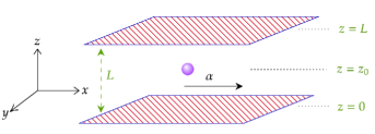
Figure 1: Uniformly accelerated atom confined to a cavity.

Inside the cavity the atomic trajectory is given by

$$t(\tau)=\frac{1}{\alpha}\sinh(\alpha\tau),\,\,\,x(\tau)=\frac{1}{\alpha}\cosh(\alpha\tau),\,\,\,y=0,\,\,z=z_{0}\,.$$ (20)

Using the above trajectories in eq.(19), the Wightman function becomes

$$G^{+}(x(\tau),x(\tau^{\prime}))=-\frac{\alpha^{2}}{16\pi^{2}}\displaystyle\sum_{n=-\infty}^{\infty}\left[\frac{1}{\sinh^{2}\left[\frac{1}{2}(\alpha\Delta\tau-i\varepsilon)\right]-\frac{1}{4}d_{1}^{2}\alpha^{2}}-\frac{1}{\sinh^{2}\left[\frac{1}{2}(\alpha\Delta\tau-i\varepsilon)\right]-\frac{1}{4}d_{2}^{2}\alpha^{2}}\right]$$ (21)

with $d_{1}=nL,\,d_{2}=2z_{0}-nL$. Substituting the Wightman function, eq. (21) into eq.(8), the transition rate from the initial state $|i\rangle$ to the final state $|f\rangle$ is given by

$$\mathcal{R}_{|i\rangle\rightarrow|f\rangle}= -\frac{\lambda^{2}|m_{fi}|^{2}\alpha^{2}}{16\pi^{2}}\displaystyle\sum_{n=-\infty}^{\infty}\left[\int_{-\infty}^{+\infty}d(\Delta\tau)\,e^{-i\Delta E\Delta\tau}\frac{1}{\sinh^{2}\left[\frac{1}{2}(\alpha\Delta\tau-i\varepsilon)\right]-\frac{1}{4}d_{1}^{2}\alpha^{2}}\right.\,$$

$$-\left.\int_{-\infty}^{+\infty}d(\Delta\tau)\,e^{-i\Delta E\Delta\tau}\frac{1}{\sinh^{2}\left[\frac{1}{2}(\alpha\Delta\tau-i\varepsilon)\right]-\frac{1}{4}d_{2}^{2}\alpha^{2}}\right]\,.$$ (22)

Simplifying the above equation through a contour integral as shown in the Appendix A, the rate of transition from the initial state $|i\rangle$ to the final state $|f\rangle$ can be written as

$$\mathcal{R}_{|i\rangle\rightarrow|f\rangle}= \lambda^{2}|m_{fi}|^{2}\left[\theta\,(-\Delta E)\left\{\frac{|\Delta E|}{2\pi}+\mathfrak{f}\left(|\Delta E|,\,\alpha,\,\frac{L}{2}\right)-\mathfrak{h}\left(|\Delta E|,\,\alpha,\,z_{0},\frac{L}{2}\right)\right\}\left(1+\frac{1}{\exp{\frac{2\pi|\Delta E|}{\alpha}}-1}\right)\right.$$

$$+\left.\theta\,(\Delta E)\left\{\frac{\Delta E}{2\pi}+\mathfrak{f}\left(\Delta E,\,\alpha,\,\frac{L}{2}\right)-\mathfrak{h}\left(\Delta E,\,\alpha,\,z_{0},\frac{L}{2}\right)\right\}\left(\frac{1}{\exp{\frac{2\pi\Delta E}{\alpha}}-1}\right)\right]$$ (23)

where we have defined

$$\mathfrak{f}\left(\Delta E,\,\alpha,\,\frac{L}{2}\right) =2\displaystyle\sum_{n=1}^{\infty}\mathfrak{g}\left(\Delta E,\,\alpha,\,\frac{nL}{2}\right)$$ (24)

$$\mathfrak{h}\left(\Delta E,\,\alpha,\,z_{0}\,,\frac{L}{2}\right) =\displaystyle\sum_{n=-\infty}^{\infty}\mathfrak{g}\left(\Delta E,\,\alpha,\,z_{0}-\frac{nL}{2}\right)\,$$ (25)

where $\mathfrak{g}\left(\Delta E,\,\alpha,\,z_{0}\right)$ is defined as

$$\mathfrak{g}\left(\Delta E,\,\alpha,\,z_{0}\right)=\frac{\sin(\frac{2\Delta E}{\alpha}\sinh^{-1}(\alpha z_{0}))}{4\pi z_{0}\sqrt{1+\alpha^{2}z_{0}^{2}}}\,.$$ (26)

Hence, from the above result the upward and downward transition rates can be written as

$$\mathcal{R}_{|g\rangle\rightarrow|e\rangle}=\lambda^{2}\left[\left\{\frac{\omega_{0}}{2\pi}+\mathfrak{f}\left(\omega_{0},\,\alpha,\,\frac{L}{2}\right)-\mathfrak{h}\left(\omega_{0},\,\alpha,\,z_{0},\frac{L}{2}\right)\right\}\left(\frac{1}{\exp{\frac{2\pi\omega_{0}}{\alpha}}-1}\right)\right]$$ (27)

$$\mathcal{R}_{|e\rangle\rightarrow|g\rangle}=\lambda^{2}\left[\left\{\frac{\omega_{0}}{2\pi}+\mathfrak{f}\left(\omega_{0},\,\alpha,\,\frac{L}{2}\right)-\mathfrak{h}\left(\omega_{0},\,\alpha,\,z_{0},\frac{L}{2}\right)\right\}\left(1+\frac{1}{\exp{\frac{2\pi\omega_{0}}{\alpha}}-1}\right)\right]\,.$$ (28)

Note that the ratio of the upward and the downward transition rates in the cavity scenario is identical with the free space result (eq.(18)).

Next, in order to describe the single boundary and free space cases, we take the limiting cases of the above expressions. Taking the limit $L\rightarrow\infty$, we find that in eq.(s)(27, 28) only the $n=0$ term survives from the infinite summation terms, and one can effectively reduce the cavity scenario to a situation where only one reflecting boundary exists. Hence, using this limit, the upward and downward transition rates in the presence of a single reflecting boundary turn out to be

$$\mathcal{R}_{|g\rangle\rightarrow|e\rangle}=\lambda^{2}\left[\left\{\frac{\omega_{0}}{2\pi}-\mathfrak{g}\left(\omega_{0},\,\alpha,\,z_{0}\right)\right\}\left(\frac{1}{\exp{2\pi\omega_{0}/\alpha}-1}\right)\right]$$ (29)

$$\mathcal{R}_{|e\rangle\rightarrow|g\rangle}=\lambda^{2}\left[\left\{\frac{\omega_{0}}{2\pi}-\mathfrak{g}\left(\omega_{0},\,\alpha,\,z_{0}\right)\right\}\left(1+\frac{1}{\exp{2\pi\omega_{0}/\alpha}-1}\right)\right]\,.$$ (30)

On the other hand, taking the limits $L\rightarrow\infty$ and $z_{0}\rightarrow\infty$ together, eq.(s)(27, 28) lead to the expression for the upward and downward transition rates in the free space given by eq.(s)(16, 17).

We now investigate the variation of the transition rate of a single two level atom (from its ground state energy level $|g\rangle$ to the excited state energy level $|e\rangle$) confined to a cavity with the length of the cavity ($L$), distance of the atom from the boundary ($z_{0}$), and the atomic acceleration ($\alpha$). The findings are plotted below, where all physical quantities are expressed in dimensionless units.

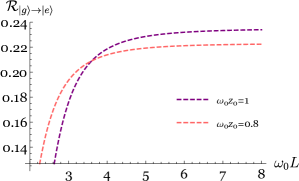
Figure 2: Transition rate from $|g\rangle\rightarrow|e\rangle$ (per unit $\frac{\lambda^{2}\omega_{0}}{2\pi}$) versus separation between the two boundaries, $\alpha/\omega_{0}=4$.

Figure 2 shows the variation of the transition rate from $|g\rangle\rightarrow|e\rangle$ (per unit $\frac{\lambda^{2}\omega_{0}}{2\pi}$) with respect to the length of the cavity (separation between the two boundaries) for different values of distance of the atom from one boundary. From the plots, it can be seen that for a fixed value of the initial atomic distance $z_{0}$ from one boundary, the transition rate get enhanced when the cavity length increases and attains a maximum value for large values of $L$ ($\omega_{0}L>>\omega_{0}z_{0}$). This is expected since more number of field modes take part in the interaction between the scalar field and the atom after increasing the cavity length, which in turn increases the transition rate. When $\omega_{0}L>>\omega_{0}z_{0}$, the cavity scenario reduces to the case of a single boundary, and hence, the upward transition rate reaches a constant value. It is also observed that the upper value of the rate is more for a larger value of $\omega_{0}z_{0}$.

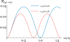
Figure 3: Transition rate from $|g\rangle\rightarrow|e\rangle$ (per unit $\frac{\lambda^{2}\omega_{0}}{2\pi}$) versus distance of the atom from one boundary, $\alpha/\omega_{0}=4$.

Figure 3 shows the variation of the transition rate from $|g\rangle\rightarrow|e\rangle$ (per unit $\frac{\lambda^{2}\omega_{0}}{2\pi}$) with respect to the distance of the atom from one boundary for different values of the length of the cavity, for a fixed value of acceleration. From the plots, it is observed that for a fixed value of the length of the cavity $L$, when we increase the atomic distance from one boundary, transition rate shows an oscillatory behaviour and vanishes if either the atom touches any one of the boundaries or if the atom is equidistant from both boundaries. It can also be observed (as we have seen earlier in Fig 2) that with increase in the length of the cavity ($L$), the rate of upward transition increases.

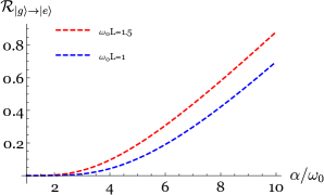
Figure 4: Transition rate from $|g\rangle\rightarrow|e\rangle$ (per unit $\frac{\lambda^{2}\omega_{0}}{2\pi}$) versus acceleration, $\omega_{0}z_{0}=0.3$.

Figure 4 shows the variation of the transition rate from $|g\rangle\rightarrow|e\rangle$ (per unit $\frac{\lambda^{2}\omega_{0}}{2\pi}$) with respect to the acceleration of the atom for different values of the length of the cavity and distance of the atom from one boundary. From the plots, it is observed that for a fixed value of the length of the cavity $L$ and the atomic distance $z_{0}$ from one boundary, the transition rate increases when the acceleration of the atom is increased. Once again we find that the transition rate is more for a larger value of the cavity length which is consistent with our earlier observations.

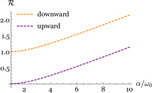
(a) In free space

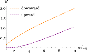
(b) Inside the cavity for a fixed value of $\omega_{0}L=3,\,\omega_{0}z_{0}=0.6$

Figure 5: Transition rate (per unit $\frac{\lambda^{2}\omega_{0}}{2\pi}$) versus acceleration.

In Figure 5, we compare the upward and the downward transition rates with respect to the atomic acceleration for two cases, namely, atom in free space (Figure 5), atom confined to a cavity (Figure 5). From the above plots, it is seen that both the transition rates get affected due to the presence of the cavity. As noted earlier, in presence of the cavity the upward and the downward transition rates decrease with decrease in the cavity length. Here it is seen that when $\omega_{0}L\sim\omega_{0}z_{0}$, the cavity effect is strong enough to reduce sharply the downward transition rate.

At this point, it might be interesting to make a quantitative estimation of the transition rate for the case when a single atom is placed inside a cavity. Following [73], we choose the length of the cavity in the order of $100nm$, distance between the atom and the nearest boundary in the order of $20nm$, and the acceleration in the order of $10^{17}m/s^{2}$. The energy gap between the ground and excited state of a single Rubidium atom $Rb^{87}$ is of the order of $0.25eV$ [88]. Now using eq.(27) with $\lambda=0.1$, and the above values, the upward transition rate of the single atom inside a cavity turns out to be $3.38\times 10^{-12}eV=5.12\times 10^{3}s^{-1}$. This tells us that in order to observe a transition to the excited state from the ground state in $1ns$, one would need to perform an experiment with a collection of $10^{6}$ atoms.

4 Transition rates of a single atom from the viewpoint of a coaccelerated observer

In this section, the transitions of a uniformly accelerated atom is analysed from the perspective of a coaccelerated observer. The coaccelerated observer will perceive the atom as being static. Hence, the observer will see no Unruh acceleration radiation as there is no relative acceleration between the observer and the atom. However, for the observer to detect acceleration radiation, the field is assumed to be at an arbitrary temperature $T$. To calculate the transition rates and see the boundary effects on the transitions of the uniformly accelerated atom, we consider that the coordinates of the coaccelerated frame are the Rindler coordinates $(\tau,\,\eta,\,y,\,z)$ with the following relation with those of the laboratory coordinates ($t,\,x,\,y,\,z$)

$$t(\tau,\eta)=\frac{1}{\alpha}e^{\alpha\eta}\sinh(\alpha\tau),\,\,\,x(\tau,\eta)=\frac{1}{\alpha}e^{\alpha\eta}\cosh(\alpha\tau)\,.$$ (31)

In the coaccelerated frame, the field operator $\phi(x(\tau))$ is replaced by its Rindler counterpart $\bar{\phi}(x(\tau))$ [81] and it takes the form [38]

$$\bar{\phi}(\tau,\mathbf{x}))=\int_{0}^{\infty}d\omega\int_{-\infty}^{\infty}dk_{y}\int_{-\infty}^{\infty}dk_{z}\left[b_{\omega,k_{y},k_{z}}\mathcal{V}_{\omega,k_{y},k_{z}}(\tau,\mathbf{x})+b^{\dagger}_{\omega,k_{y},k_{z}}\mathcal{V}^{\star}_{\omega,k_{y},k_{z}}(\tau,\mathbf{x})\right]$$ (32)

with

$$\mathcal{V}_{\omega,k_{y},k_{z}}(\tau,\mathbf{x})=\sqrt{\frac{\sinh(\pi\omega/\alpha)}{4\pi^{4}\alpha}}\mathcal{K}_{i\frac{\omega}{\alpha}}\left(\frac{k_{\perp}}{\alpha}e^{\alpha\eta}\right)e^{-i\omega\tau+ik_{y}y+ik_{z}z}$$ (33)

being the positive frequency orthonormal mode solution, $\mathcal{K}_{\nu}(x)$ is the Bessel function of imaginary argument and $k_{\perp}\equiv|\mathbf{k}_{\perp}|=\sqrt{k_{y}^{2}+k_{z}^{2}}$. The interaction between the atom and the scalar field in this case can be written as [81]

$$H=\lambda m(\tau)\bar{\phi}(x(\tau))\,.$$ (34)

As mentioned earlier, in order to determine the transition rate in the coaccelerated frame, we consider that the field is at an arbitrary temperature $T$. As the thermal state is a mixed state, therefore to calculate the response of a single atom coupled to the massless scalar field, it is further assumed that the field state can be represented by a pure state $|\sigma_{\omega,k_{y},k_{z}}\rangle$ with a probability factor $p_{\sigma}(\omega)=e^{-\beta\omega\sigma}/N(\omega)$ with $\beta=1/T$ and $N(\omega)=\displaystyle\sum_{\sigma=0}^{\infty}e^{-\beta\omega\sigma}$. In this case, $|\psi_{\pm},\,\sigma_{\omega,k_{y},k_{z}}\rangle$ and $|E_{n},\,\gamma_{\omega^{\prime},k^{\prime}_{y},k^{\prime}_{z}}\rangle$ can be used to represent respectively, the initial and the final state of the atom-field system.

Now, following the procedure described in the previous section, the transition probability of the atom-field system from the initial state $|i\rangle$ to final state $|f\rangle$ is given by

$$\mathcal{P}^{\beta}_{|i\rangle\rightarrow|f\rangle}=\lambda^{2}|m_{fi}|^{2}F^{\beta}(\Delta E)\,,$$ (35)

where the response function $F^{\beta}(\Delta E)$ is defined as

$$F^{\beta}(\Delta E)=\int_{-\infty}^{+\infty}d\tau\int_{-\infty}^{+\infty}d\tau^{\prime}\,e^{-i\Delta E(\tau-\tau^{\prime})}\,G_{\beta}^{+}(x(\tau),x(\tau^{\prime}))$$ (36)

and

$$G^{+}_{\beta}(x(\tau),x(\tau^{\prime}))=\frac{tr[\rho^{\prime}\phi(x(\tau))\phi(x(\tau^{\prime})]}{tr[\rho^{\prime}]}$$

$$=N^{-1}(\omega)\displaystyle\sum_{\sigma=0}^{\infty}\int_{0}^{\infty}d\omega\int_{-\infty}^{\infty}dk_{y}\int_{-\infty}^{\infty}dk_{z}e^{-\beta\omega\sigma}\langle\sigma_{\omega,k_{y},k_{z}}|\bar{\phi}(x(\tau))\bar{\phi}(x(\tau^{\prime}))|\sigma_{\omega,k_{y},k_{z}}\rangle$$ (37)

is the positive frequency Wightman function of the scalar field in a thermal state at an arbitrary temperature $T$ in the coaccelerated frame. Exploiting the time translational invariance property of the positive frequency Wightman function, the response function per unit proper time can be written as

$$\mathcal{F}^{\beta}(\Delta E)=\int_{-\infty}^{+\infty}d(\Delta\tau)\,e^{-i\Delta E\Delta\tau}\,G^{+}_{\beta}(x(\tau),x(\tau^{\prime}))\,.$$ (38)

Therefore, the transition probability per unit proper time of the atom from the initial state $|i\rangle$ to the final state $|f\rangle$ turns out to be

$$\mathcal{R}^{\beta}_{|i\rangle\rightarrow|f\rangle}=\lambda^{2}|m_{fi}|^{2}\mathcal{F}^{\beta}(\Delta E)\,.$$ (39)

4.1 Transition rates in empty space with respect to a coaccelerated observer

Using eq.(32) in eq.(37), the thermal Wightman function takes the following form for an arbitrary temperature $T$,

$$G^{+}_{\beta}(x(\tau),x(\tau^{\prime}))$$

$$=\int_{0}^{\infty}d\omega\int_{-\infty}^{\infty}dk_{y}\int_{-\infty}^{\infty}dk_{z}\bigg{[}\displaystyle\sum_{\sigma=0}^{\infty}(\sigma+1)e^{-\beta\omega\sigma}\mathcal{V}_{\omega,k_{y},k_{z}}(\tau,\mathbf{x})\mathcal{V}^{\star}_{\omega,k_{y},k_{z}}(\tau^{\prime},\mathbf{x}^{\prime})\bigg{.}$$

$$+\bigg{.}\displaystyle\sum_{\sigma=1}^{\infty}\sigma e^{-\beta\omega\sigma}\mathcal{V}^{\star}_{\omega,k_{y},k_{z}}(\tau,\mathbf{x})\mathcal{V}_{\omega,k_{y},k_{z}}(\tau^{\prime},\mathbf{x}^{\prime})\bigg{]}\bigg{/}\displaystyle\sum_{\sigma=0}^{\infty}e^{-\beta\omega\sigma}$$

$$=\int_{0}^{\infty}d\omega\int_{-\infty}^{\infty}dk_{y}\int_{-\infty}^{\infty}dk_{z}\bigg{[}\frac{e^{\omega/T}}{e^{\omega/T}-1}\mathcal{V}_{\omega,k_{y},k_{z}}(\tau,\mathbf{x})\mathcal{V}^{\star}_{\omega,k_{y},k_{z}}(\tau^{\prime},\mathbf{x}^{\prime})\bigg{.}$$

$$+\bigg{.}\frac{1}{e^{\omega/T}-1}\mathcal{V}^{\star}_{\omega,k_{y},k_{z}}(\tau,\mathbf{x})\mathcal{V}_{\omega,k_{y},k_{z}}(\tau^{\prime},\mathbf{x}^{\prime})\bigg{]}\,.$$ (40)

In the Rindler coordinates, the trajectory of the atom can be described by

$$t=\tau,\,\,\,\eta=y=z=0\,.$$ (41)

Using eq.(s)(33, 41) in eq.(40), the thermal Wightman function takes the form

$$G^{+}_{\beta}(x(\tau),x(\tau^{\prime}))$$

$$=\frac{1}{4\pi^{4}\alpha}\int_{0}^{\infty}d\omega\int_{-\infty}^{\infty}dk_{y}\int_{-\infty}^{\infty}dk_{z}\sinh\left(\frac{\pi\omega}{\alpha}\right)\mathcal{K}_{i\omega/\alpha}^{2}\left(\frac{k_{\perp}}{\alpha}\right)\bigg{[}\frac{e^{\omega/T}}{e^{\omega/T}-1}e^{-i\omega(\tau-\tau^{\prime})}\bigg{.}$$

$$+\bigg{.}\frac{1}{e^{\omega/T}-1}e^{i\omega(\tau-\tau^{\prime})}\bigg{]}$$ (42)

$$=\frac{1}{4\pi^{2}}\int_{0}^{\infty}d\omega\,\omega\bigg{[}\frac{e^{\omega/T}}{e^{\omega/T}-1}e^{-i\omega(\tau-\tau^{\prime})}+\bigg{.}\frac{1}{e^{\omega/T}-1}e^{i\omega(\tau-\tau^{\prime})}\bigg{]}$$

$$=-\frac{1}{4\pi^{2}}\displaystyle\sum_{s=-\infty}^{\infty}\frac{1}{(\Delta\tau-is\beta-i\varepsilon)^{2}}$$ (43)

where in the second line, we have used the integral

$$\int_{-\infty}^{\infty}dk_{y}\int_{-\infty}^{\infty}dk_{z}\mathcal{K}_{i\omega/\alpha}^{2}\left(\frac{k_{\perp}}{\alpha}\right)=\frac{\alpha\pi^{2}\omega}{\sinh(\pi\omega/\alpha)}\,.$$ (44)

By inserting the above Wightman function into eq.(s)(38, 39), and performing integrations using the contour integration method, the upward and downward transition rates of a single atom submerged in the thermal bath turn out to be, respectively

$$\mathcal{R}^{\beta}_{|g\rangle\rightarrow|e\rangle}=\frac{\lambda^{2}\omega_{0}}{2\pi}\left(\frac{1}{\exp(\omega_{0}/T)-1}\right)$$ (45)

$$\mathcal{R}^{\beta}_{|e\rangle\rightarrow|g\rangle}=\frac{\lambda^{2}\omega_{0}}{2\pi}\left(1+\frac{1}{\exp(\omega_{0}/T)-1}\right)\,.$$ (46)

The above equations suggest that in the coaccelerated frame both the upward and the downward transition can occur for an atom immersed in the thermal bath which is very similar to the transitions observed by an instantaneous inertial observer. Taking the limit $T\rightarrow 0$, we can see that the upward transition rate vanishes and this is consistent with the fact that there should be no transition if the observer is static with respect to the atom. Eq.(s)(16, 17, 45, 46) clearly indicate that the transition rates of an uniformly accelerated atom seen by an instantaneously inertial observer and by a coaccelerated observer are identical only when if we take the thermal bath temperature in the coaccelerated frame to be $T=\alpha/2\pi$.

4.2 Transition rates in a cavity from the viewpoint of a coaccelerated observer

In this subsection, we consider a uniformly accelerated atom interacting with a vacuum massless scalar field confined to a cavity of length $L$ from the perspective of a coaccelerated observer. We assume that perfectly reflecting boundaries are placed at $z=0$ and $z=L$. In a coaccelerated frame, this scenario will be depicted as a static atom interacting with a massless scalar field in a thermal state at an arbitrary temperature $T$ inside a cavity of length $L$.

In case of a single reflecting boundary, the scalar field obeys the Dirichlet boundary condition $\phi|_{z=0}=0$. The positive frequency Rindler mode function for the massless scalar field takes the form

$$\mathcal{V}_{\omega,k_{y},k_{z}}(\tau,\mathbf{x})=\sqrt{\frac{\sinh(\pi\omega/\alpha)}{2\pi^{4}\alpha}}\mathcal{K}_{i\frac{\omega}{\alpha}}\left(\frac{k_{\perp}}{\alpha}e^{\alpha\eta}\right)\sin(k_{z}z)e^{-i\omega\tau+ik_{y}y}\,.$$ (47)

Inserting eq.(47) in eq.(40), the thermal Wightman function takes the form

$$G^{+}_{\beta}(x(\tau),x(\tau^{\prime}))$$

$$=\frac{1}{4\pi^{4}\alpha}\int_{0}^{\infty}d\omega\int_{-\infty}^{\infty}dk_{y}\int_{-\infty}^{\infty}dk_{z}\sinh\left(\frac{\pi\omega}{\alpha}\right)\mathcal{K}_{i\omega/\alpha}\left(\frac{k_{\perp}}{\alpha}e^{\alpha\eta}\right)\mathcal{K}_{i\omega/\alpha}\left(\frac{k_{\perp}}{\alpha}e^{\alpha\eta^{\prime}}\right)\bigg{\{}\cos\big{[}k_{z}(z-z^{\prime})\big{]}\bigg{.}$$

$$-\bigg{.}\cos\big{[}k_{z}(z+z^{\prime})\big{]}\bigg{\}}\times\bigg{[}\frac{e^{\omega/T}}{e^{\omega/T}-1}e^{-i\omega(\tau-\tau^{\prime})+ik_{y}(y-y^{\prime})}+\frac{1}{e^{\omega/T}-1}e^{i\omega(\tau-\tau^{\prime})-ik_{y}(y-y^{\prime})}\bigg{]}\,.$$ (48)

Now for the cavity scenario, the Dirichlet boundary condition obeyed by the scalar field is $\phi|_{z=0}=\phi|_{z=L}=0$. Using the above boundary condition (eq.(48)) and by using the method of images, the thermal Wightman function of the massless scalar field confined to the cavity turns out to be

$$G^{+}_{\beta}(x(\tau),x(\tau^{\prime}))$$

$$=\frac{1}{4\pi^{4}\alpha}\displaystyle\sum_{n=-\infty}^{\infty}\int_{0}^{\infty}d\omega\int_{-\infty}^{\infty}dk_{y}\int_{-\infty}^{\infty}dk_{z}\sinh\left(\frac{\pi\omega}{\alpha}\right)\mathcal{K}_{i\omega/\alpha}\left(\frac{k_{\perp}}{\alpha}e^{\alpha\eta}\right)\mathcal{K}_{i\omega/\alpha}\left(\frac{k_{\perp}}{\alpha}e^{\alpha\eta^{\prime}}\right)$$

$$\times\bigg{\{}\cos\big{[}k_{z}(z-z^{\prime}-nL)\big{]}-\cos\big{[}k_{z}(z+z^{\prime}-nL)\big{]}\bigg{\}}\bigg{[}\frac{e^{\omega/T}}{e^{\omega/T}-1}e^{-i\omega(\tau-\tau^{\prime})+ik_{y}(y-y^{\prime})}\bigg{.}$$

$$+\bigg{.}\frac{1}{e^{\omega/T}-1}e^{i\omega(\tau-\tau^{\prime})-ik_{y}(y-y^{\prime})}\bigg{]}\,.$$ (49)

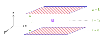
Figure 6: Static atom confined to a cavity.

Inside the cavity, the atomic trajectory becomes

$$t=\tau,\,\,\,\eta=y=0,\,\,z=z_{0}\,.$$ (50)

Inserting the above trajectory in eq.(49), using the result [38]

$$\int_{-\infty}^{\infty}dk_{y}\int_{-\infty}^{\infty}dk_{z}\mathcal{K}_{i\omega/\alpha}^{2}\left(\frac{k_{\perp}}{\alpha}\right)\cos\left[2k_{z}\frac{d}{2}\right]=\frac{\alpha\pi^{2}}{\sinh(\pi\omega/\alpha)}\frac{\sin\left(\frac{2\omega}{\alpha}\sinh^{-1}\left(\frac{d\alpha}{2}\right)\right)}{d\sqrt{1+\frac{1}{4}\alpha^{2}d^{2}}}$$ (51)

and following the procedure mentioned in the previous subsection, the thermal Wightman function becomes

$$G^{+}_{\beta}(x(\tau),x(\tau^{\prime}))=-\frac{1}{4\pi^{2}}\displaystyle\sum_{n=-\infty}^{\infty}\displaystyle\sum_{s=-\infty}^{\infty}\left[\frac{\mathcal{B}_{1}}{\mathcal{C}_{1}}\frac{1}{(\Delta\tau-is\beta-i\varepsilon)^{2}-\mathcal{B}_{1}^{2}}-\frac{\mathcal{B}_{2}}{\mathcal{C}_{2}}\frac{1}{(\Delta\tau-is\beta-i\varepsilon)^{2}-\mathcal{B}_{2}^{2}}\right]$$ (52)

with

$$\mathcal{B}_{1} =\frac{2}{\alpha}\sinh^{-1}\left(\frac{nL\alpha}{2}\right)$$

$$\mathcal{C}_{1} =nL\sqrt{1+\frac{1}{4}\alpha^{2}n^{2}L^{2}}$$

$$\mathcal{B}_{2} =\frac{2}{\alpha}\sinh^{-1}\left(\alpha\left(z_{0}-\frac{nL}{2}\right)\right)$$

$$\mathcal{C}_{2} =(2z_{0}-nL)\sqrt{1+\frac{1}{4}\alpha^{2}(2z_{0}-nL)^{2}}\,.$$

Putting the above Wightman function in eq.(s)(38, 39), and performing the integrations using the contour integration technique, the downward and upward transition rates of the single atom system submerged in the thermal bath read, respectively

$$\mathcal{R}_{|g\rangle\rightarrow|e\rangle}=\lambda^{2}\left[\left\{\frac{\omega_{0}}{2\pi}+\mathfrak{f}\left(\omega_{0},\,\alpha,\,\frac{L}{2}\right)-\mathfrak{h}\left(\omega_{0},\,\alpha,\,z_{0},\frac{L}{2}\right)\right\}\left(\frac{1}{\exp(\omega_{0}/T)-1}\right)\right]$$ (53)

$$\mathcal{R}_{|e\rangle\rightarrow|g\rangle}=\lambda^{2}\left[\left\{\frac{\omega_{0}}{2\pi}+\mathfrak{f}\left(\omega_{0},\,\alpha,\,\frac{L}{2}\right)-\mathfrak{h}\left(\omega_{0},\,\alpha,\,z_{0},\frac{L}{2}\right)\right\}\left(1+\frac{1}{\exp(\omega_{0}/T)-1}\right)\right]\,.$$ (54)

Next, taking the limit $L\rightarrow\infty$, the upward and the downward transition rate in the presence of a single reflecting boundary turn out respectively to be

$$\mathcal{R}_{|g\rangle\rightarrow|e\rangle}=\lambda^{2}\left[\left\{\frac{\omega_{0}}{2\pi}-\mathfrak{g}\left(\omega_{0},\,\alpha,\,z_{0}\right)\right\}\left(\frac{1}{\exp{\omega_{0}/T}-1}\right)\right]$$ (55)

$$\mathcal{R}_{|e\rangle\rightarrow|g\rangle}=\lambda^{2}\left[\left\{\frac{\omega_{0}}{2\pi}-\mathfrak{g}\left(\omega_{0},\,\alpha,\,z_{0}\right)\right\}\left(1+\frac{1}{\exp{\omega_{0}/T}-1}\right)\right]$$ (56)

with $\mathfrak{f}\left(\omega_{0},\,\alpha,\,\frac{L}{2}\right)$, $\mathfrak{h}\left(\omega_{0},\,\alpha,\,z_{0},\,\frac{L}{2}\right)$ and $\mathfrak{g}\left(\omega_{0},\,\alpha,\,z_{0}\right)$ being the same as in eq.(s)(24, 25) and eq.(26).

The above analysis clearly displays the similarity between the transitions observed by an instantaneously inertial observer and a coaccelerated observer in a thermal bath for both the upward and the downward transition rates when the atom is confined in a cavity. Here too we notice that taking the thermal bath temperature in the coaccelerated frame $T=\alpha/2\pi$, eq.(s)(53, 54, 27, 28) indicate that the transition rates of a uniformly accelerated atom seen by a coaccelerated observer in a thermal bath and by an instantaneously inertial observer are identical inside the cavity.

5 Coupling of the two-atom system with a massless scalar field

We consider two identical atoms $A$ and $B$ and assume that they are travelling along synchronous trajectories in a vacuum with massless scalar field fluctuations, the interatomic distance is assumed to be constant and the proper times of the two atoms can be described by the same time $\tau$ [80]. In the laboratory frame, trajectories of the two atoms can be represented through $x_{A}(\tau)$ and $x_{B}(\tau)$. Here we consider each atom as a two level system having energy levels $-\omega_{0}/2$ and $+\omega_{0}/2$. Therefore, the entire two-atom system can be described by the three energy levels with energies $-\omega_{0},\,0\,\,\text{and}\,\,\omega_{0}$ [89]. We designate them by $E_{n}$ with $n=1,2,3$. The low and high energy levels associated with eigenstates are $|E_{1}\rangle=|g_{A},g_{B}\rangle$ and $|E_{3}\rangle=|e_{A},e_{B}\rangle$ where $|g\rangle$ and $|e\rangle$ represent the ground state and the excited state of a single atom respectively. The energy level $E_{2}$ is degenerate corresponding to the eigenstates $|g_{A},e_{B}\rangle$ and $|e_{A},g_{B}\rangle$.

In the instantaneously inertial frame, the Hamiltonian describing the atom-field interaction is given by

$$H=\lambda\Big{[}m_{A}(\tau)\phi(x_{A}(\tau))+m_{B}(\tau)\phi(x_{B}(\tau))\Big{]}\,,$$ (57)

where $\lambda$ is the atom-field coupling constant assumed to be very small. The forms of $\phi(x(\tau))$ and $m(\tau)$ are the same as given in eq.(s)(2, 3). As a result of the atom-field interaction, transitions also occur for the two-atom system. According to the time-dependent perturbation theory in the first-order approximation, the transition amplitude for the atom-field system to transit from the initial state $|\chi,0_{M}\rangle$ to the final state $|\chi^{\prime},\phi_{f}\rangle$ is given by

$$\mathcal{A}_{|\chi,0_{M}\rangle\rightarrow|\chi^{\prime},\phi_{f}\rangle}=i\lambda\langle\chi^{\prime},\phi_{f}|\int_{-\infty}^{+\infty}m_{A}(\tau)\phi(x_{A}(\tau))|\chi,0_{M}\rangle+A\rightleftharpoons B\,\text{term}\,.$$ (58)

Squaring the above transition amplitude and summing over all possible field states, the transition probability from the initial state $|\chi\rangle$ to the final state $|\chi^{\prime}\rangle$ can be written as

$$\mathcal{P}_{|\chi\rangle\rightarrow|\chi^{\prime}\rangle}=\lambda^{2}\Big{[}|m^{(A)}_{\chi^{\prime}\chi}|^{2}F_{AA}(\Delta E)+m^{(B)}_{\chi^{\prime}\chi}\,m^{(A)\,*}_{\chi^{\prime}\chi}F_{AB}(\Delta E)\Big{]}+A\rightleftharpoons B\,\text{terms}\,,$$ (59)

where $m^{(A)}_{\chi^{\prime}\chi}=\langle\chi^{\prime}|m(0)\otimes\mathds{1}_{B}|\chi\rangle$, and $m^{(B)}_{\chi^{\prime}\chi}=\langle\chi^{\prime}|\mathds{1}_{A}\otimes m(0)|\chi\rangle$. The response function $F_{\xi\xi^{\prime}}(\Delta E)$ is defined as

$$F_{\xi\xi^{\prime}}(\Delta E)=\int_{-\infty}^{+\infty}d\tau\int_{-\infty}^{+\infty}d\tau^{\prime}\,e^{-i\Delta E(\tau-\tau^{\prime})}\,G^{+}(x_{\xi}(\tau),x_{\xi^{\prime}}(\tau^{\prime}))$$ (60)

with $\xi,\xi^{\prime}$ can be labeled by $A$ or $B$, and

$$G^{+}(x_{\xi}(\tau),x_{\xi^{\prime}}(\tau^{\prime}))=\langle 0_{M}|\phi(x_{\xi}(\tau))\phi(x_{\xi^{\prime}}(\tau^{\prime}))|0_{M}\rangle$$ (61)

is the Wightman function of the massless scalar field. From equation (59) it is seen that for the two-atom system, the transition probability carries two terms one of them of which is associated with only one of the atoms and other one associated with both the atoms.

Exploiting the time translational invariance property of the Wightman function, the response function per unit proper time can be written as

$$\mathcal{F}_{\xi\xi^{\prime}}(\Delta E)=\int_{-\infty}^{+\infty}d(\Delta\tau)\,e^{-i\Delta E\Delta\tau}\,G^{+}(x_{\xi}(\tau),x_{\xi^{\prime}}(\tau^{\prime}))$$ (62)

where $\Delta\tau=\tau-\tau^{\prime}$. Therefore, the transition probability per unit proper time of the two-atom system from the initial state $|\chi\rangle$ to the final state $|\chi^{\prime}\rangle$ turns out to be

$$\mathcal{R}_{|\chi\rangle\rightarrow|\chi^{\prime}\rangle}=\lambda^{2}\Big{[}|m^{(A)}_{\chi^{\prime}\chi}|^{2}\mathcal{F}_{AA}(\Delta E)+m^{(B)}_{\chi^{\prime}\chi}\,m^{(A)\,*}_{\chi^{\prime}\chi}\mathcal{F}_{AB}(\Delta E)\Big{]}+A\rightleftharpoons B\,\text{terms}\,.$$ (63)

The existence of the cross terms in the above equation indicates that the rate of transition between the two neighbouring energy levels is not only related to the sum of the rates of transition of the two atoms, but also to their cross-correlation.

In the following section, this formalism is used to examine the rate of transitions of a two-atom system under various conditions of uniform acceleration and contact with the vacuum massless scalar field. The correlation between two atoms can be considered as a factor which can affect the transition rate of a two-atom system. In practice, entanglement is not always maintained during experimental conditions, and non-maximally entangled states are frequently used as resources or probes. This motivates us to consider non-maximally entangled states, as well, in our analysis. The general pure quantum state of the two-atom system is given by [73]

$$|\psi\rangle=\sin\theta|g_{A},e_{B}\rangle+\cos\theta|e_{A},g_{B}\rangle$$ (64)

where the entanglement parameter $\theta$ lies in the range $0\leq\theta\leq\pi$. The above quantum state becomes a separable state for the values of $\theta=0,\pi/2,\pi$ and represents the maximally entangled state for the value $\theta=\pi/4$ (superradiant state), and $\theta=3\pi/4$ (subradiant state). Considering the above generic entangled quantum state as the initial state in the following section, we explore how the non-inertial motion of the atoms, nature of the observer, type of the background field and the presence of the boundaries affect the rate of transition of the two-atom system.

6 Transition rates of the two-atom system from the viewpoint of a local inertial observer

In this part, we analyse the transitions of a uniformly accelerated two-atom system prepared in any generic entangled state $|\psi\rangle$ that interacts with the vacuum massless scalar field from the perspective of a locally inertial observer. To see the boundary effects on the transitions of the uniformly accelerated two-atom system in this scenario, several cases have been studied in the following subsections.

6.1 Transition rates for entangled atoms in empty space with respect to a local inertial observer

Here we evaluate the transition rates of a two-atom system that is uniformly accelerating while interacting with a vacuum massless scalar field in the absence of any perfectly reflecting boundary. In the laboratory frame, trajectories of both the atoms read

$$t_{A}(\tau)=t_{B}(\tau)=\frac{1}{\alpha}\sinh(\alpha\tau),\,\,\,x_{A}(\tau)=x_{B}(\tau)=\frac{1}{\alpha}\cosh(\alpha\tau),\,\,\,y_{B}=y_{A}+d,\,\,\,z_{A}=z_{B}=0\,,$$ (65)

where $d$, $\alpha$ and $\tau$ denote the constant interatomic distance, proper acceleration and the proper time of the two-atom system.

Using the scalar field operator eq.(2) in eq.(61), the Wightman function becomes [80]

$$G^{+}(x_{\xi}(\tau),x_{\xi^{\prime}}(\tau^{\prime}))$$

$$= -\frac{1}{4\pi^{2}}\frac{1}{(t_{\xi}(\tau)-t_{\xi^{\prime}}(\tau^{\prime})-i\varepsilon)^{2}-(x_{\xi}(\tau)-x_{\xi^{\prime}}(\tau^{\prime}))^{2}-(y_{\xi}(\tau)-y_{\xi^{\prime}}(\tau^{\prime}))^{2}-(z_{\xi}(\tau)-z_{\xi^{\prime}}(\tau^{\prime}))^{2}}\,.$$ (66)

Substituting the trajectories (eq.(65)) in eq.(66), the Wightman function turns out to be

$$G^{+}(x_{\xi}(\tau),x_{\xi^{\prime}}(\tau^{\prime}))=-\frac{\alpha^{2}}{16\pi^{2}}\frac{1}{\sinh^{2}\left[\frac{1}{2}(\alpha\Delta\tau-i\varepsilon)\right]}$$ (67)

with $\Delta\tau=\tau-\tau^{\prime}$ for $\xi=\xi^{\prime}$, and

$$G^{+}(x_{\xi}(\tau),x_{\xi^{\prime}}(\tau^{\prime}))=-\frac{\alpha^{2}}{16\pi^{2}}\frac{1}{\sinh^{2}\left[\frac{1}{2}(\alpha\Delta\tau-i\varepsilon)\right]-\frac{1}{4}d^{2}\alpha^{2}}$$ (68)

for $\xi\neq\xi^{\prime}$. Substituting the Wightman functions (eq.(s)(67, 68)) into eq.(60) and eq.(63), the transition rate of the two-atom system from the initial state $|\psi\rangle$ to the final state $|E_{n}\rangle$ can be expressed as

$$\mathcal{R}_{|\psi\rangle\rightarrow|E_{n}\rangle}=\lambda^{2}\Big{[} |m^{(A)}_{E_{n}\psi}|^{2}\mathcal{F}_{AA}(\Delta E)+|m^{(B)}_{E_{n}\psi}|^{2}\mathcal{F}_{BB}(\Delta E)+m^{(B)}_{E_{n}\psi}\,m^{(A)\,*}_{E_{n}\psi}\mathcal{F}_{AB}(\Delta E)$$

$$+m^{(A)}_{E_{n}\psi}\,m^{(B)\,*}_{E_{n}\psi}\mathcal{F}_{BA}(\Delta E)\Big{]}$$ (69)

with

$$\mathcal{F}_{\xi\xi^{\prime}}(\Delta E)=-\frac{\alpha^{2}}{16\pi^{2}}\int_{-\infty}^{+\infty}d(\Delta\tau)\,e^{-i\Delta E\Delta\tau}\frac{1}{\sinh^{2}\left[\frac{1}{2}(\alpha\Delta\tau-i\varepsilon)\right]}$$ (70)

for $\xi=\xi^{\prime}$ and

$$\mathcal{F}_{\xi\xi^{\prime}}(\Delta E)=-\frac{\alpha^{2}}{16\pi^{2}}\int_{-\infty}^{+\infty}d(\Delta\tau)\,e^{-i\Delta E\Delta\tau}\frac{1}{\sinh^{2}\left[\frac{1}{2}(\alpha\Delta\tau-i\varepsilon)\right]-\frac{1}{4}d^{2}\alpha^{2}}$$ (71)

for $\xi\neq\xi^{\prime}$. We simplify the transition rate (eq.(69)) by performing contour integration, leading to

$$\mathcal{R}_{|\psi\rangle\rightarrow|E_{n}\rangle}= \lambda^{2}\left\{\theta\,(-\Delta E)\left(\frac{|\Delta E|}{2\pi}+\frac{\sin 2\theta\sin(\frac{2|\Delta E|}{\alpha}\sinh^{-1}(\frac{1}{2}\alpha d))}{2\pi d\sqrt{1+\frac{1}{4}d^{2}\alpha^{2}}}\right)\left(1+\frac{1}{e^{2\pi|\Delta E|/\alpha}-1}\right)\right.$$

$$+\left.\theta\,(\Delta E)\left(\frac{\Delta E}{2\pi}+\frac{\sin 2\theta\sin(\frac{2\Delta E}{\alpha}\sinh^{-1}(\frac{1}{2}\alpha d))}{2\pi d\sqrt{1+\frac{1}{4}d^{2}\alpha^{2}}}\right)\left(\frac{1}{e^{2\pi\Delta E/\alpha}-1}\right)\right\}$$ (72)

where $\theta(\Delta E)$ is the Heaviside step function defined as

$$\theta(\Delta E)=\begin{cases}1,\,\,\,\Delta E>0,\\ 0,\,\,\,\Delta E<0.\end{cases}$$ (73)

It follows that the two transition processes, namely, the upward and downward transition can take place for the two-atom system under uniform acceleration with the upward transition rate given by

$$\mathcal{R}_{|\psi\rangle\rightarrow|e_{A}e_{B}\rangle}=\lambda^{2}\left\{\left(\frac{\omega_{0}}{2\pi}+\frac{\sin 2\theta\sin(\frac{2\omega_{0}}{\alpha}\sinh^{-1}(\frac{1}{2}\alpha d))}{2\pi d\sqrt{1+\frac{1}{4}d^{2}\alpha^{2}}}\right)\left(\frac{1}{\exp{2\pi\omega_{0}/\alpha}-1}\right)\right\}\,,$$ (74)

and the downward transition rate given by

$$\mathcal{R}_{|\psi\rangle\rightarrow|g_{A}g_{B}\rangle}=\lambda^{2}\left\{\left(\frac{\omega_{0}}{2\pi}+\frac{\sin 2\theta\sin(\frac{2\omega_{0}}{\alpha}\sinh^{-1}(\frac{1}{2}\alpha d))}{2\pi d\sqrt{1+\frac{1}{4}d^{2}\alpha^{2}}}\right)\left(1+\frac{1}{\exp{2\pi\omega_{0}/\alpha}-1}\right)\right\}\,.$$ (75)

Interestingly, the ratio of the upward and the downward transition rates for the two-atom case is identical with that of the single atom case (eq.(18)).

6.2 Transition rates for entangled atoms in a cavity with respect to a local inertial observer

Here we consider that a uniformly accelerated two-atom system interacts with a vacuum massless scalar field confined in a cavity having length $L$. Assuming that the two atoms are moving parallel to the boundary (see Fig. 7) with their proper acceleration similar to the previous case, we investigate the effect of the cavity on the transition rates.

Assuming the scalar field obeys the Dirichlet boundary condition $\phi|_{z=0}=\phi|_{z=L}=0$, and using the method of images, the Wightman function of the massless scalar field confined to the cavity of length $L$ takes the form

$$G^{+}(x_{\xi}(\tau),x_{\xi^{\prime}}(\tau^{\prime}))$$

$$= -\frac{1}{4\pi^{2}}\displaystyle\sum_{n=-\infty}^{\infty}\left[\frac{1}{(t_{\xi}(\tau)-t_{\xi^{\prime}}(\tau^{\prime})-i\varepsilon)^{2}-(x_{\xi}(\tau)-x_{\xi^{\prime}}(\tau^{\prime}))^{2}-(y_{\xi}(\tau)-y_{\xi^{\prime}}(\tau^{\prime}))^{2}-(z_{\xi}(\tau)-z_{\xi^{\prime}}(\tau^{\prime})-nL)^{2}}\right.$$

$$\left.-\frac{1}{(t_{\xi}(\tau)-t_{\xi^{\prime}}(\tau^{\prime})-i\varepsilon)^{2}-(x_{\xi}(\tau)-x_{\xi^{\prime}}(\tau^{\prime}))^{2}-(y_{\xi}(\tau)-y_{\xi^{\prime}}(\tau^{\prime}))^{2}-(z_{\xi}(\tau)+z_{\xi^{\prime}}(\tau^{\prime})-nL)^{2}}\right]$$ (76)

To represent the atomic trajectories in terms of the atomic proper time $\tau$, we choose the Cartesian coordinates in the laboratory frame so that boundaries are fixed at $z=0$ and $z=L$.

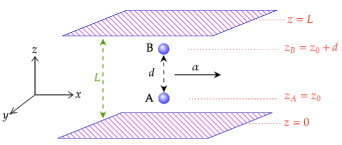
Figure 7: Uniformly accelerated two-atom confined in a cavity.

Considering that the inter-atomic distance $d$ remains perpendicular while two atoms are moving parallel to the boundary with their proper acceleration, the atomic trajectories are given by

$$t_{A/B}(\tau)=\frac{1}{\alpha}\sinh(\alpha\tau),\,\,\,x_{A/B}(\tau)=\frac{1}{\alpha}\cosh(\alpha\tau),\,\,\,y_{A/B}=y_{0},\,\,z_{A}=z_{0},\,\,z_{B}=z_{0}+d\,.$$ (77)

Using the above trajectories in eq.(76), the Wightman function becomes

$$G^{+}(x_{\xi}(\tau),x_{\xi^{\prime}}(\tau^{\prime}))=-\frac{\alpha^{2}}{16\pi^{2}}\displaystyle\sum_{n=-\infty}^{\infty}\left[\frac{1}{\sinh^{2}\left[\frac{1}{2}(\alpha\Delta\tau-i\varepsilon)\right]-\frac{1}{4}d_{1}^{2}\alpha^{2}}-\frac{1}{\sinh^{2}\left[\frac{1}{2}(\alpha\Delta\tau-i\varepsilon)\right]-\frac{1}{4}d_{2}^{2}\alpha^{2}}\right]$$ (78)

for $\xi=\xi^{\prime}$, with $d_{1}=nL,\,d_{2}=2z_{\xi}-nL$ and

$$G^{+}(x_{\xi}(\tau),x_{\xi^{\prime}}(\tau^{\prime}))=-\frac{\alpha^{2}}{16\pi^{2}}\displaystyle\sum_{n=-\infty}^{\infty}\left[\frac{1}{\sinh^{2}\left[\frac{1}{2}(\alpha\Delta\tau-i\varepsilon)\right]-\frac{1}{4}d_{3}^{2}\alpha^{2}}-\frac{1}{\sinh^{2}\left[\frac{1}{2}(\alpha\Delta\tau-i\varepsilon)\right]-\frac{1}{4}d_{4}^{2}\alpha^{2}}\right]$$ (79)

for $\xi\neq\xi^{\prime}$, with $d_{3}=-d-nL$ (for $\xi=A,\xi^{\prime}=B$); $d_{3}=d-nL$ (for $\xi=B,\xi^{\prime}=A$) and $d_{4}=2z_{0}+d-nL$.

Using the above Wightman functions, the rate of transition from the initial state $|\psi\rangle$ to the final state $|E_{n}\rangle$ can be written as

$$\mathcal{R}_{|\psi\rangle\rightarrow|E_{n}\rangle}=\lambda^{2}\displaystyle\sum_{n=-\infty}^{\infty}\Big{[} |m^{(A)}_{E_{n}\psi}|^{2}\mathcal{F}_{AA}(\Delta E)+|m^{(B)}_{E_{n}\psi}|^{2}\mathcal{F}_{BB}(\Delta E)+m^{(B)}_{E_{n}\psi}\,m^{(A)\,*}_{E_{n}\psi}\mathcal{F}_{AB}(\Delta E)$$

$$+m^{(A)}_{E_{n}\psi}\,m^{(B)\,*}_{E_{n}\psi}\mathcal{F}_{BA}(\Delta E)\Big{]}$$ (80)

with

$$\mathcal{F}_{\xi\xi^{\prime}}(\Delta E)=-\frac{\alpha^{2}}{16\pi^{2}}\int_{-\infty}^{+\infty}d(\Delta\tau)\,e^{-i\Delta E\Delta\tau}\left[\frac{1}{\sinh^{2}\left[\frac{1}{2}(\alpha\Delta\tau-i\varepsilon)\right]-\frac{1}{4}d_{1}^{2}\alpha^{2}}-\frac{1}{\sinh^{2}\left[\frac{1}{2}(\alpha\Delta\tau-i\varepsilon)\right]-\frac{1}{4}d_{2}^{2}\alpha^{2}}\right]$$ (81)

for $\xi=\xi^{\prime}$ and

$$\mathcal{F}_{\xi\xi^{\prime}}(\Delta E)=-\frac{\alpha^{2}}{16\pi^{2}}\int_{-\infty}^{+\infty}d(\Delta\tau)\,e^{-i\Delta E\Delta\tau}\left[\frac{1}{\sinh^{2}\left[\frac{1}{2}(\alpha\Delta\tau-i\varepsilon)\right]-\frac{1}{4}d_{3}^{2}\alpha^{2}}-\frac{1}{\sinh^{2}\left[\frac{1}{2}(\alpha\Delta\tau-i\varepsilon)\right]-\frac{1}{4}d_{4}^{2}\alpha^{2}}\right]$$ (82)

for $\xi\neq\xi^{\prime}$. Eq.(80) can be further simplified by performing contour integration to obtain

$$\mathcal{R}_{|\psi\rangle\rightarrow|E_{n}\rangle}= \lambda^{2}\left\{\theta\,(-\Delta E)\left(\frac{|\Delta E|}{2\pi}+\mathfrak{f}\left(|\Delta E|,\,\alpha,\,\frac{L}{2}\right)-\cos^{2}\theta\,\mathfrak{h}\left(|\Delta E|,\,\alpha,\,z_{0},\,\frac{L}{2}\right)-\sin^{2}\theta\,\right.\right.$$

$$\times\left.\mathfrak{m}\left(|\Delta E|,\,\alpha,\,z_{0},\,d,\,\frac{L}{2}\right)+\sin 2\theta\,\mathfrak{n}\left(|\Delta E|,\,\alpha,\,\frac{d}{2},\,\frac{L}{2}\right)-\sin 2\theta\right.$$

$$\times\left.\mathfrak{m}\left(|\Delta E|,\,\alpha,\,z_{0},\,\frac{d}{2},\,\frac{L}{2}\right)\right)\left(1+\frac{1}{\exp{2\pi|\Delta E|/\alpha}-1}\right)$$

$$+\theta\,(\Delta E)\left(\frac{\Delta E}{2\pi}+\mathfrak{f}\left(\Delta E,\,\alpha,\,\frac{L}{2}\right)-\cos^{2}\theta\,\mathfrak{h}\left(\Delta E,\,\alpha,\,z_{0},\,\frac{L}{2}\right)-\sin^{2}\theta\,\right.$$

$$\times\left.\mathfrak{m}\left(\Delta E,\,\alpha,\,z_{0},\,d,\,\frac{L}{2}\right)+\sin 2\theta\,\mathfrak{n}\left(\Delta E,\,\alpha,\,\frac{d}{2},\,\frac{L}{2}\right)-\sin 2\theta\right.$$

$$\times\left.\left.\mathfrak{m}\left(\Delta E,\,\alpha,\,z_{0},\,\frac{d}{2},\,\frac{L}{2}\right)\right)\left(\frac{1}{\exp{2\pi\Delta E/\alpha}-1}\right)\right\}$$ (83)

where we have defined

$$\mathfrak{f}\left(\Delta E,\,\alpha,\,\frac{L}{2}\right) =2\displaystyle\sum_{n=1}^{\infty}\mathfrak{g}\left(\Delta E,\,\alpha,\,\frac{nL}{2}\right)\,$$ (84)

$$\mathfrak{h}\left(\Delta E,\,\alpha,\,z_{0}\,,\frac{L}{2}\right) =\displaystyle\sum_{n=-\infty}^{\infty}\mathfrak{g}\left(\Delta E,\,\alpha,\,z_{0}-\frac{nL}{2}\right)\,$$ (85)

$$\mathfrak{m}\left(\Delta E,\,\alpha,\,z_{0}\,,d,\,\frac{L}{2}\right) =\displaystyle\sum_{n=-\infty}^{\infty}\mathfrak{g}\left(\Delta E,\,\alpha,\,z_{0}+d-\frac{nL}{2}\right)\,$$ (86)

$$\mathfrak{n}\left(\Delta E,\,\alpha,\,\frac{d}{2},\,\frac{L}{2}\right) =\displaystyle\sum_{n=-\infty}^{\infty}\mathfrak{g}\left(\Delta E,\,\alpha,\,\frac{d-nL}{2}\right)\,$$ (87)

and $\mathfrak{g}\left(\Delta E,\,\alpha,\,z_{0}\right)$ is defined as

$$\mathfrak{g}\left(\Delta E,\,\alpha,\,z_{0}\right)=\frac{\sin(\frac{2\Delta E}{\alpha}\sinh^{-1}(\alpha z_{0}))}{4\pi z_{0}\sqrt{1+\alpha^{2}z_{0}^{2}}}\,.$$ (88)

From the above equation it follows that the two transition processes can take place for the two-atom system in the presence of a reflecting boundary with the upward transition rate given by

$$\mathcal{R}_{|\psi\rangle\rightarrow|e_{A}e_{B}\rangle}= \lambda^{2}\left\{\left(\frac{\omega_{0}}{2\pi}+\mathfrak{f}\left(\omega_{0},\,\alpha,\,\frac{L}{2}\right)-\cos^{2}\theta\,\mathfrak{h}\left(\omega_{0},\,\alpha,\,z_{0},\frac{L}{2}\right)-\sin^{2}\theta\,\right.\right.$$

$$\times\left.\mathfrak{m}(\omega_{0},\,\alpha,\,z_{0},\,d,\,\frac{L}{2})+\sin 2\theta\,\mathfrak{n}\left(\omega_{0},\,\alpha,\,\frac{d}{2},\,\frac{L}{2}\right)-\sin 2\theta\right.$$

$$\times\left.\left.\mathfrak{m}\left(\omega_{0},\,\alpha,\,z_{0},\,\frac{d}{2},\,\frac{L}{2}\right)\right)\left(\frac{1}{\exp{2\pi\omega_{0}/\alpha}-1}\right)\right\}$$ (89)

and the downward transition rate given by

$$\mathcal{R}_{|\psi\rangle\rightarrow|g_{A}g_{B}\rangle}= \lambda^{2}\left\{\left(\frac{\omega_{0}}{2\pi}+\mathfrak{f}\left(\omega_{0},\,\alpha,\,\frac{L}{2}\right)-\cos^{2}\theta\,\mathfrak{h}\left(\omega_{0},\,\alpha,\,z_{0},\frac{L}{2}\right)-\sin^{2}\theta\,\right.\right.$$

$$\times\left.\mathfrak{m}(\omega_{0},\,\alpha,\,z_{0},\,d,\,\frac{L}{2})+\sin 2\theta\,\mathfrak{n}\left(\omega_{0},\,\alpha,\,\frac{d}{2},\,\frac{L}{2}\right)-\sin 2\theta\right.$$

$$\times\left.\left.\mathfrak{m}\left(\omega_{0},\,\alpha,\,z_{0},\,\frac{d}{2},\,\frac{L}{2}\right)\right)\left(1+\frac{1}{\exp{2\pi\omega_{0}/\alpha}-1}\right)\right\}\,.$$ (90)

In order to obtain the single mirror and free space scenarios, we now take the limiting cases of these expressions. Taking the limit $L\rightarrow\infty$, we find that eq.(s)(6.2, 6.2) reduce to the expression for the upward and the downward transition rate in the presence of a single reflecting boundary

$$\mathcal{R}_{|\psi\rangle\rightarrow|e_{A}e_{B}\rangle}= \lambda^{2}\Bigg{\{}\left(\frac{\omega_{0}}{2\pi}-\cos^{2}\theta\,\mathfrak{g}(\omega_{0},\,\alpha,\,z_{0})-\sin^{2}\theta\,\mathfrak{g}(\omega_{0},\,\alpha,\,(z_{0}+d))\right.\Bigg{.}$$

$$+\left.\left.\sin 2\theta\left(\mathfrak{g}\left(\omega_{0},\,\alpha,\,\frac{d}{2}\right)-\mathfrak{g}\left(\omega_{0},\,\alpha,\,z_{0}+\frac{d}{2}\right)\right)\right)\left(\frac{1}{\exp{2\pi\omega_{0}/\alpha}-1}\right)\right\}$$ (91)

$$\mathcal{R}_{|\psi\rangle\rightarrow|g_{A}g_{B}\rangle}= \lambda^{2}\Bigg{\{}\left(\frac{\omega_{0}}{2\pi}-\cos^{2}\theta\,\mathfrak{g}(\omega_{0},\,\alpha,\,z_{0})-\sin^{2}\theta\,\mathfrak{g}(\omega_{0},\,\alpha,\,(z_{0}+d))\right.\Bigg{.}$$

$$+\left.\left.\sin 2\theta\left(\mathfrak{g}\left(\omega_{0},\,\alpha,\,\frac{d}{2}\right)-\mathfrak{g}\left(\omega_{0},\,\alpha,\,z_{0}+\frac{d}{2}\right)\right)\right)\left(1+\frac{1}{\exp{2\pi\omega_{0}/\alpha}-1}\right)\right\}$$ (92)

It may be noted that the above relations resemble those of the single boundary results given in [80] but they are not identical as in our case the interatomic distance is perpendicular to the reflecting boundary whereas in [80] the interatomic distance is parallel to the reflecting boundary. Similarly, taking the limits $L\rightarrow\infty$ and $z_{0}\rightarrow\infty$, eq.(s)(6.2, 6.2) lead to the expressions for the upward and the downward transition rate in free space given by eq.(s)(74, 75).

We now study the variation of the transition rate of an entangled two atom system from an initial entangled state $|\psi\rangle$ to a product state with higher energy value $|e_{A}e_{B}\rangle$ confined to a cavity with the atomic acceleration ($\alpha$), length of the cavity ($L$), distance of any one atom from one boundary ($z_{0}$), entanglement parameter ($\theta$), and the interatomic distance ($d$). The findings are plotted below, where all physical quantities are expressed in dimensionless units. Since cavity effects are significant when the length scales are comparable [90], hence we choose a similar order of magnitude for $\omega_{0}L,\,\omega_{0}z_{0}\,\text{and}\,\omega_{0}d$. In Figure 8, we show the behaviour of the transition rate with respect to the entanglement parameter for the cases where the atoms are in free space, in the vicinity of a single boundary and inside a cavity.

(a) Upward transition rate

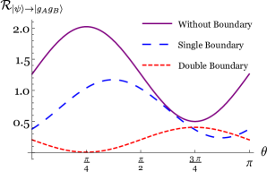
(b) Downward transition rate

Figure 8: Transition rate (per unit $\frac{\lambda^{2}\omega_{0}}{2\pi}$) versus entanglement parameter for a fixed value of $\alpha/\omega_{0}=4,\,\omega_{0}d=0.5,\,\omega_{0}L=1.2,\,\omega_{0}z_{0}=0.2$.

From the above Figure, it can be seen that the transition rate $|\psi\rangle\rightarrow|e_{A}e_{B}\rangle$ (per unit $\frac{\lambda^{2}\omega_{0}}{2\pi}$) varies sinusoidally with the entanglement parameter $\theta$. In free space, the transition rate increases (from the case corresponding to the zero entanglement product state) with increase in the entanglement parameter and it becomes maximum when the initial state is maximally entangled ($\theta=\pi/4$ super-radiant state). Further increment of the entanglement parameter decreases the transition rate and it becomes minimum at $\theta=3\pi/4$ (sub-radiant state). In the vicinity of a single boundary, behaviour of the transition rate is quite similar to the free space scenario, with a slight shifting of the extremum points). Surprisingly, inside the cavity, the behaviour of the transition rate is opposite to the free space scenario. The transition rate decreases with the increase in entanglement parameter and it vanishes at $\theta=\pi/4$. Thus, the $\theta=\pi/4$ state exhibits a subradiant behaviour for the cavity set up. Further increment of entanglement parameter increases the transition rate and it becomes maximum at $\theta=3\pi/4$. Note also, that around $\theta=3\pi/4$, the values of the transition rate corresponding to cases of empty space, single boundary, and two boundaries, are nearly the same.

Figure 8 for the downward transition rates shows a similar behaviour with respect to the entanglement parameter. The only difference is that the magnitude of the downward transition rate is greater than the upward transition rate. From both the Figures, it is observed that when the initial entangled state is the super-radiant maximally entangled state ($\theta=\pi/4$), then there is no upward or downward transition inside a cavity. Therefore, this observation indicates that for this value of the entanglement parameter, the entanglement of the initial state is preserved.

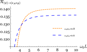
Figure 9: Transition rate from $|\psi\rangle\rightarrow|e_{A}e_{B}\rangle$ (per unit $\frac{\lambda^{2}\omega_{0}}{2\pi}$) versus separation between two boundaries, $\alpha/\omega_{0}=4$.

Figure 9 shows the variation of the transition rate from $|\psi\rangle\rightarrow|e_{A}e_{B}\rangle$ (per unit $\frac{\lambda^{2}\omega_{0}}{2\pi}$) with respect to the length of the cavity for different values of distance of any one atom from one boundary. From the plots, it can be seen that for a fixed value of the initial atomic distance $z_{0}$ of any one atom from the nearest boundary, the transition rate get enhanced when the cavity length increases and attains a maximum value for large values of $L$ ($\omega_{0}L>>\omega_{0}z_{0}$). This behaviour is similar to that of the single atom case, as mentioned earlier. As more number of field modes take part in the interaction between the scalar field and the atoms due to the increased cavity length, the transition rate increases. When $\omega_{0}L>>\omega_{0}z_{0}$, the cavity scenario reduces to a single boundary set up and hence the upward transition rate takes a constant value. It is also observed that the saturation value of the transition rate is more for a larger value of $\omega_{0}z_{0}$.

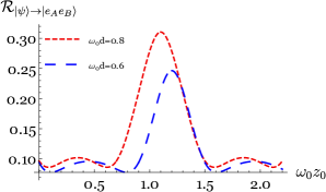
Figure 10: Transition rate from $|\psi\rangle\rightarrow|e_{A}e_{B}\rangle$ (per unit $\frac{\lambda^{2}\omega_{0}}{2\pi}$) versus distance of any one atom from one boundary, $\alpha/\omega_{0}=4,\,\omega_{0}L=3$.

Figure 10 shows the variation of the transition rate from $|\psi\rangle\rightarrow|e_{A}e_{B}\rangle$ (per unit $\frac{\lambda^{2}\omega_{0}}{2\pi}$) with respect to the distance of any one atom from one boundary $\omega_{0}z_{0}$ for different interatomic distances $\omega_{0}d$. From the plots, it is observed that for a fixed value of the interatomic distance and cavity length, the transition rate is much smaller when the atoms are close to the any one of the boundaries. Thereafter, with increase of the atomic distance from one boundary, the transition rate rises sharply and reaches maximum when the distance of both atoms to their nearest boundaries are equal. The importance of boundary effects are thereby clearly exhibited. From the plot, it is also seen that increasing the interatomic distance increases the upward transition rate for a fixed cavity length.

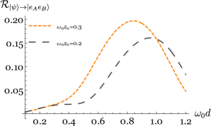
Figure 11: Transition rate from $|\psi\rangle\rightarrow|e_{A}e_{B}\rangle$ (per unit $\frac{\lambda^{2}\omega_{0}}{2\pi}$) versus interatomic distance, $\alpha/\omega_{0}=4,\,\omega_{0}L=1.5$.

Figure 11 shows the variation of the transition rate from $|\psi\rangle\rightarrow|e_{A}e_{B}\rangle$ (per unit $\frac{\lambda^{2}\omega_{0}}{2\pi}$) with respect to the interatomic distance for different values of distance of any one atom from one boundary. From the plots, we see that for a fixed atomic distance from one boundary and cavity length, transition rate initially increases when the interatomic distance increases. After a certain value of interatomic distance, increasing the distance between the two atoms further make them move closer to the boundary and hence due to boundary effects, the transition rate falls down.

Figure 12: Transition rate from $|\psi\rangle\rightarrow|e_{A}e_{B}\rangle$ (per unit $\frac{\lambda^{2}\omega_{0}}{2\pi}$) versus acceleration, $\omega_{0}d=0.5,\,\omega_{0}z_{0}=0.3$.

Figure 12 shows the variation of the transition rate from $|\psi\rangle\rightarrow|e_{A}e_{B}\rangle$ (per unit $\frac{\lambda^{2}\omega_{0}}{2\pi}$) with respect to the atomic acceleration for different values of cavity length. Similar to the single atom case, it is seen that when the atomic acceleration is increased, the transition rate also increases and the rate of transition depends on the cavity length. This is expected since acceleration radiation should increase with increase in acceleration.

(a) In free space

(b) Inside the cavity for a fixed value of $\omega_{0}L=4,\,\omega_{0}z_{0}=1$

Figure 13: Transition rate (per unit $\frac{\lambda^{2}\omega_{0}}{2\pi}$) versus acceleration for a fixed value of $\theta=3\pi/4,\,\omega_{0}d=0.5$.

In Figure 13, we have plotted the upward and the downward transition rates with respect to the atomic acceleration for two cases, namely, two atoms are in free space (Figure 13), two atoms are confined to a cavity (Figure 13). A comparison of the two plots reveals that the downward transition rate can get diminished for a suitable choice of parameters when the atoms are inside the cavity. The upward transitions in both cases are driven by the acceleration, as is clear from the corresponding expresions, as well.

Before going to the next section, we present a quantitative estimation of the upward transition rate for the two-atom system, composed of two Rubidium atoms $Rb^{87}$ placed inside a cavity. Following [73], we choose the length of the cavity in the order of $100nm$, distance between any one atom and the nearest boundary in the order of $20nm$, interatomic distance in the order of $30nm$, energy gap between the most generic entangled state and excited state of the two-atom system is of the order of $0.5eV$, and the acceleration in the order of $10^{17}m/s^{2}$. Using eq.(6.2) with the coupling constant $\lambda=0.1$, taking the entanglement parameter $\theta=3\pi/4$ for the maximally entangled state, and the above values, the upward transition rate of the uniformly accelerated two-atom system inside a cavity becomes $3.75\times 10^{-12}eV=5.68\times 10^{3}s^{-1}$.

7 Transition rates of the two-atom system from the viewpoint of a coaccelerated observer

In this section, the transitions of a uniformly accelerated two-atom system prepared in any generic entangled state $|\psi\rangle$ that interacts with a massless scalar field is analysed from the perspective of a coaccelerated observer. To see the boundary effects on the transitions of the uniformly accelerated two-atom system in this scenario, we consider that the coordinate of the coaccelerated frame will be the Rindler coordinate $(\tau,\,\eta,\,y,\,z)$ with the relation with those of the laboratory coordinates ($t,\,x,\,y,\,z$) being given by

$$t(\tau,\eta)=\frac{1}{\alpha}e^{\alpha\eta}\sinh(\alpha\tau),\,\,\,x(\tau,\eta)=\frac{1}{\alpha}e^{\alpha\eta}\cosh(\alpha\tau)\,.$$ (93)

In the coaccelerated frame, the field operator $\phi(x(\tau))$ is replaced by its Rindler counterpart $\bar{\phi}(x(\tau))$ and takes the form

$$\bar{\phi}(\tau,\mathbf{x}))=\int_{0}^{\infty}d\omega\int_{-\infty}^{\infty}dk_{y}\int_{-\infty}^{\infty}dk_{z}\left[b_{\omega,k_{y},k_{z}}\mathcal{V}_{\omega,k_{y},k_{z}}(\tau,\mathbf{x})+b^{\dagger}_{\omega,k_{y},k_{z}}\mathcal{V}^{\star}_{\omega,k_{y},k_{z}}(\tau,\mathbf{x})\right]$$ (94)

with

$$\mathcal{V}_{\omega,k_{y},k_{z}}(\tau,\mathbf{x})=\sqrt{\frac{\sinh(\pi\omega/\alpha)}{4\pi^{4}\alpha}}\mathcal{K}_{i\frac{\omega}{\alpha}}\left(\frac{k_{\perp}}{\alpha}e^{\alpha\eta}\right)e^{-i\omega\tau+ik_{y}y+ik_{z}z}$$ (95)

being the positive frequency orthonormal mode solution, $\mathcal{K}_{\nu}(x)$ is the Bessel function of imaginary argument and $k_{\perp}\equiv|\mathbf{k}_{\perp}|=\sqrt{k_{y}^{2}+k_{z}^{2}}$. The interaction between the atoms and the scalar field is given by [81]

$$H=\lambda\Big{[}m_{A}(\tau)\bar{\phi}(x_{A}(\tau))+m_{B}(\tau)\bar{\phi}(x_{B}(\tau))\Big{]}\,.$$ (96)

To determine the transition rate of the two-atom system in the coaccelerated frame, we a thermal field at an arbitrary temperature $T$. As the thermal state is a mixed state, in order to calculate the response of the two atoms coupled to the massless scalar field, additionally it is assumed that the field state can be represented by a pure state $|\sigma_{\omega,k_{y},k_{z}}\rangle$ with a probability factor $p_{\sigma}(\omega)=e^{-\beta\omega\sigma}/N(\omega)$ with $\beta=1/T$ and $N(\omega)=\displaystyle\sum_{\sigma=0}^{\infty}e^{-\beta\omega\sigma}$. In this case, $|\psi,\,\sigma_{\omega,k_{y},k_{z}}\rangle$ and $|E_{n},\,\gamma_{\omega^{\prime},k^{\prime}_{y},k^{\prime}_{z}}\rangle$ can be used to represent the initial and the final state of the atom-field system.

Following the procedure described in the previous sections, the probability that the atom-field system will transit from initial state $|\psi\rangle$ to final state $|E_{n}\rangle$ is then given by

$$\mathcal{P}_{|\psi_{\pm}\rangle\rightarrow|E_{n}\rangle}=\lambda^{2}\Big{[}|m^{(A)}_{E_{n}\psi_{\pm}}|^{2}F^{\beta}_{AA}(\Delta E)+m^{(B)}_{E_{n}\psi_{\pm}}\,m^{(A)\,*}_{E_{n}\psi_{\pm}}F^{\beta}_{AB}(\Delta E)\Big{]}+A\rightleftharpoons B\,\text{terms}\,.$$ (97)

The response function $F^{\beta}_{\xi\xi^{\prime}}(\Delta E)$ is defined as

$$F^{\beta}_{\xi\xi^{\prime}}(\Delta E)=\int_{-\infty}^{+\infty}d\tau\int_{-\infty}^{+\infty}d\tau^{\prime}\,e^{-i\Delta E(\tau-\tau^{\prime})}\,G^{+}_{\beta}(x_{\xi}(\tau),x_{\xi^{\prime}}(\tau^{\prime}))$$ (98)

with $\xi,\xi^{\prime}$ labeled by $A$ or $B$, and

$$G^{+}_{\beta}(x_{\xi}(\tau),x_{\xi^{\prime}}(\tau^{\prime}))=\frac{tr[\rho^{\prime}\phi(x_{\xi}(\tau))\phi(x_{\xi^{\prime}}(\tau^{\prime})]}{tr[\rho^{\prime}]}$$

$$=N^{-1}(\omega)\displaystyle\sum_{\sigma=0}^{\infty}\int_{0}^{\infty}d\omega\int_{-\infty}^{\infty}dk_{y}\int_{-\infty}^{\infty}dk_{z}e^{-\beta\omega\sigma}\langle\sigma_{\omega,k_{y},k_{z}}|\bar{\phi}(x_{\xi}(\tau))\bar{\phi}(x_{\xi^{\prime}}(\tau^{\prime}))|\sigma_{\omega,k_{y},k_{z}}\rangle$$ (99)

is the positive frequency Wightman function of the scalar field in a thermal state at an arbitrary temperature $T$ in the coaccelerated frame. Exploiting the time translational invariance property of the Wightman function, the response function per unit proper time can be written as

$$\mathcal{F}^{\beta}_{\xi\xi^{\prime}}(\Delta E)=\int_{-\infty}^{+\infty}d(\Delta\tau)\,e^{-i\Delta E\Delta\tau}\,G^{+}_{\beta}(x_{\xi}(\tau),x_{\xi^{\prime}}(\tau^{\prime}))\,.$$ (100)

Therefore, the transition probability per unit proper time of the two-atom system from the initial state $|\chi\rangle$ to the final state $|\chi^{\prime}\rangle$ turns out to be

$$\mathcal{R}^{\beta}_{|\chi\rangle\rightarrow|\chi^{\prime}\rangle}=\lambda^{2}\Big{[}|m^{(A)}_{\chi^{\prime}\chi}|^{2}\mathcal{F}^{\beta}_{AA}(\Delta E)+m^{(B)}_{\chi^{\prime}\chi}\,m^{(A)\,*}_{\chi^{\prime}\chi}\mathcal{F}^{\beta}_{AB}(\Delta E)\Big{]}+A\rightleftharpoons B\,\text{terms}\,.$$ (101)

7.1 Transition rates for entangled atoms in empty space with respect to a coaccelerated observer

Substituting eq.(94) into eq.(99), the thermal Wightman function takes the following form for an arbitrary temperature $T$:

$$G^{+}_{\beta}(x_{\xi}(\tau),x_{\xi^{\prime}}(\tau^{\prime}))$$

$$=\int_{0}^{\infty}d\omega\int_{-\infty}^{\infty}dk_{y}\int_{-\infty}^{\infty}dk_{z}\bigg{[}\displaystyle\sum_{\sigma=0}^{\infty}(\sigma+1)e^{-\beta\omega\sigma}\mathcal{V}_{\omega,k_{y},k_{z}}(\tau_{\xi},\mathbf{x}_{\xi})\mathcal{V}^{\star}_{\omega,k_{y},k_{z}}(\tau^{\prime}_{\xi^{\prime}},\mathbf{x}^{\prime}_{\xi^{\prime}})\bigg{.}$$

$$+\bigg{.}\displaystyle\sum_{\sigma=1}^{\infty}\sigma e^{-\beta\omega\sigma}\mathcal{V}^{\star}_{\omega,k_{y},k_{z}}(\tau_{\xi},\mathbf{x}_{\xi})\mathcal{V}_{\omega,k_{y},k_{z}}(\tau^{\prime}_{\xi},\mathbf{x}^{\prime}_{\xi^{\prime}})\bigg{]}\bigg{/}\displaystyle\sum_{\sigma=0}^{\infty}e^{-\beta\omega\sigma}$$

$$=\int_{0}^{\infty}d\omega\int_{-\infty}^{\infty}dk_{y}\int_{-\infty}^{\infty}dk_{z}\bigg{[}\frac{e^{\omega/T}}{e^{\omega/T}-1}\mathcal{V}_{\omega,k_{y},k_{z}}(\tau_{\xi},\mathbf{x}_{\xi})\mathcal{V}^{\star}_{\omega,k_{y},k_{z}}(\tau^{\prime}_{\xi^{\prime}},\mathbf{x}^{\prime}_{\xi^{\prime}})\bigg{.}$$

$$+\bigg{.}\frac{1}{e^{\omega/T}-1}\mathcal{V}^{\star}_{\omega,k_{y},k_{z}}(\tau_{\xi},\mathbf{x}_{\xi})\mathcal{V}_{\omega,k_{y},k_{z}}(\tau^{\prime}_{\xi},\mathbf{x}^{\prime}_{\xi^{\prime}})\bigg{]}$$ (102)

In the Rindler coordinates, the trajectories of both the atoms are given by

$$t_{A/B}=\tau,\,\,\,\eta_{A/B}=0,\,\,\,y_{A/B}=0,\,\,z_{A}=0\,\,z_{B}=d\,.$$ (103)

Substituting eq.(s)(95, 103) into eq.(102), the thermal Wightman function takes the form

$$G^{+}_{\beta}(x_{\xi}(\tau),x_{\xi^{\prime}}(\tau^{\prime}))$$

$$=\frac{1}{4\pi^{4}\alpha}\int_{0}^{\infty}d\omega\int_{-\infty}^{\infty}dk_{y}\int_{-\infty}^{\infty}dk_{z}\sinh\left(\frac{\pi\omega}{\alpha}\right)\mathcal{K}_{i\omega/\alpha}^{2}\left(\frac{k_{\perp}}{\alpha}\right)\bigg{[}\frac{e^{\omega/T}}{e^{\omega/T}-1}e^{-i\omega(\tau-\tau^{\prime})}\bigg{.}$$

$$+\bigg{.}\frac{1}{e^{\omega/T}-1}e^{i\omega(\tau-\tau^{\prime})}\bigg{]}\,.$$ (104)

Now, using following integrals

$$\int_{-\infty}^{\infty}dk_{y}\int_{-\infty}^{\infty}dk_{z}\mathcal{K}_{i\omega/\alpha}^{2}\left(\frac{k_{\perp}}{\alpha}\right)=\frac{\alpha\pi^{2}\omega}{\sinh(\pi\omega/\alpha)}$$ (105)

and

$$\int_{-\infty}^{\infty}dk_{y}\int_{-\infty}^{\infty}dk_{z}\mathcal{K}_{i\omega/\alpha}^{2}\left(\frac{k_{\perp}}{\alpha}\right)e^{-ik_{z}d}=\frac{\alpha\pi^{2}}{\sinh(\pi\omega/\alpha)}\frac{\sin\left(\frac{2\omega}{\alpha}\sinh^{-1}\left(\frac{d\alpha}{2}\right)\right)}{d\sqrt{1+\frac{1}{4}\alpha^{2}d^{2}}}$$ (106)

the thermal Wightman function takes the form

$$G^{+}_{\beta}(x_{\xi}(\tau),x_{\xi^{\prime}}(\tau^{\prime}))=-\frac{1}{4\pi^{2}}\displaystyle\sum_{s=-\infty}^{\infty}\frac{1}{(\Delta\tau-is\beta-i\varepsilon)^{2}}$$ (107)

for $\xi=\xi^{\prime}$, and

$$G^{+}_{\beta}(x_{\xi}(\tau),x_{\xi^{\prime}}(\tau^{\prime}))=-\frac{\mathcal{B}}{4\pi^{2}\mathcal{C}}\displaystyle\sum_{s=-\infty}^{\infty}\frac{1}{(\Delta\tau-is\beta-i\varepsilon)^{2}-\mathcal{B}^{2}}$$ (108)

with $\mathcal{B}=\frac{2}{\alpha}\sinh^{-1}\left(\frac{d\alpha}{2}\right)$ and $\mathcal{C}=d\sqrt{1+\frac{1}{4}\alpha^{2}d^{2}}$, for $\xi\neq\xi^{\prime}$. By inserting the aforementioned Wightman functions into eq.(s)(100, 101), and performing the integrations using contour integration, the upward and downward transition rates of the two-atom system submerged in the thermal bath turn out to be

$$\mathcal{R}^{\beta}_{|\psi\rangle\rightarrow|e_{A}e_{B}\rangle}=\lambda^{2}\left\{\left(\frac{\omega_{0}}{2\pi}+\frac{\sin 2\theta\sin(\frac{2\omega_{0}}{\alpha}\sinh^{-1}(\frac{1}{2}\alpha d))}{2\pi d\sqrt{1+\frac{1}{4}d^{2}\alpha^{2}}}\right)\left(\frac{1}{\exp{\omega_{0}/T}-1}\right)\right\}$$ (109)

$$\mathcal{R}^{\beta}_{|\psi\rangle\rightarrow|g_{A}g_{B}\rangle}=\lambda^{2}\left\{\left(\frac{\omega_{0}}{2\pi}+\frac{\sin 2\theta\sin(\frac{2\omega_{0}}{\alpha}\sinh^{-1}(\frac{1}{2}\alpha d))}{2\pi d\sqrt{1+\frac{1}{4}d^{2}\alpha^{2}}}\right)\left(1+\frac{1}{\exp{\omega_{0}/T}-1}\right)\right\}\,.$$ (110)

From the above equations it follows that in the coaccelerated frame both the upward and the downward transitions can occur for the two-atom system immersed in the thermal bath which is very similar to the transitions observed by an instantaneously inertial observer. Taking the limiting value of the temperature of the coaacelerated frame $T\rightarrow 0$, here also we can see that the upward transition rate vanishes, which is consistent with that in the Minkowski vacuum (eq.(74)). Eq.(s)(74, 75, 109, 110) indicate that the transition rates of the uniformly accelerated two-atom system in the generic entangled state seen by an instantaneously inertial observer and by a coaccelerated observer are identical only if the thermal bath temperature in the coaccelerated frame is equal to the FDU temperature $T=\alpha/2\pi$.

7.2 Transition rates for entangled atoms in a cavity with respect to a coaccelerated observer

Here we consider that a uniformly accelerated two-atom system interacts with a massless scalar field confined to a cavity of length $L$ from the perspective of a coaccelerated observer. We assume that two perfectly reflecting boundaries are placed at $z=0$ and $z=L$. As in the case of the single atom, the scenario here too depicts a static two-atom system interacting with a massless scalar field in a thermal state at an arbitrary temperature $T$ inside a cavity of length $L$.

Considering that the scalar field obeys the Dirichlet boundary condition $\phi|_{z=0}=\phi|_{z=L}=0$, and by following a similar method we have used for the single atom case, the positive frequency thermal Wightmann function of the massless scalar field confined in the cavity turns out to be

$$G^{+}_{\beta}(x_{\xi}(\tau),x_{\xi^{\prime}}(\tau^{\prime}))$$

$$=\frac{1}{4\pi^{4}\alpha}\displaystyle\sum_{n=-\infty}^{\infty}\int_{0}^{\infty}d\omega\int_{-\infty}^{\infty}dk_{y}\int_{-\infty}^{\infty}dk_{z}\sinh\left(\frac{\pi\omega}{\alpha}\right)\mathcal{K}_{i\omega/\alpha}\left(\frac{k_{\perp}}{\alpha}e^{\alpha\eta_{\xi}}\right)\mathcal{K}_{i\omega/\alpha}\left(\frac{k_{\perp}}{\alpha}e^{\alpha\eta^{\prime}_{\xi^{\prime}}}\right)$$

$$\times\bigg{\{}\cos\big{[}k_{z}(z_{\xi}-z^{\prime}_{\xi^{\prime}}-nL)\big{]}-\cos\big{[}k_{z}(z_{\xi}+z^{\prime}_{\xi^{\prime}}-nL)\big{]}\bigg{\}}\bigg{[}\frac{e^{\omega/T}}{e^{\omega/T}-1}e^{-i\omega(\tau_{\xi}-\tau^{\prime}_{\xi^{\prime}})+ik_{y}(y_{\xi}-y^{\prime}_{\xi^{\prime}})}\bigg{.}$$

$$+\bigg{.}\frac{1}{e^{\omega/T}-1}e^{i\omega(\tau_{\xi}-\tau^{\prime}_{\xi^{\prime}})-ik_{y}(y_{\xi}-y^{\prime}_{\xi^{\prime}})}\bigg{]}\,.$$ (111)

Figure 14: Static two-atom confined in a cavity.

Considering the inter-atomic distance $d$ to remain perpendicular while the two atoms are moving parallel to the boundaries with their proper acceleration, the atomic trajectories are given by

$$t_{A/B}=\tau,\,\,\,\eta_{A/B}=0,\,\,\,y_{A/B}=0,\,\,z_{A}=z_{0}\,\,z_{B}=z_{0}+d\,.$$ (112)

Inserting the above trajectories in eq.(7.2) and following the procedure mentioned in the previous subsection, the thermal Wightman function becomes

$$G^{+}_{\beta}(x_{\xi}(\tau),x_{\xi^{\prime}}(\tau^{\prime}))=-\frac{1}{4\pi^{2}}\displaystyle\sum_{n=-\infty}^{\infty}\displaystyle\sum_{s=-\infty}^{\infty}\left[\frac{\mathcal{B}_{1}}{\mathcal{C}_{1}}\frac{1}{(\Delta\tau-is\beta-i\varepsilon)^{2}-\mathcal{B}_{1}^{2}}-\frac{\mathcal{B}_{2}}{\mathcal{C}_{2}}\frac{1}{(\Delta\tau-is\beta-i\varepsilon)^{2}-\mathcal{B}_{2}^{2}}\right]$$ (113)

for $\xi=\xi^{\prime}$ with $\mathcal{B}_{1}=\frac{2}{\alpha}\sinh^{-1}\left(\frac{nL\alpha}{2}\right),\,\mathcal{C}_{1}=nL\sqrt{1+\frac{1}{4}\alpha^{2}n^{2}L^{2}},\,\mathcal{B}_{2}=\frac{2}{\alpha}\sinh^{-1}\left(\alpha\left(z_{\xi}-\frac{nL}{2}\right)\right),\,\mathcal{C}_{2}=(2z_{\xi}-nL)\sqrt{1+\frac{1}{4}\alpha^{2}(2z_{\xi}-nL)^{2}}$
and

$$G^{+}_{\beta}(x_{\xi}(\tau),x_{\xi^{\prime}}(\tau^{\prime}))=-\frac{1}{4\pi^{2}}\displaystyle\sum_{n=-\infty}^{\infty}\displaystyle\sum_{s=-\infty}^{\infty}\left[\frac{\mathcal{B}_{3}}{\mathcal{C}_{3}}\frac{1}{(\Delta\tau-is\beta-i\varepsilon)^{2}-\mathcal{B}_{3}^{2}}-\frac{\mathcal{B}_{4}}{\mathcal{C}_{4}}\frac{1}{(\Delta\tau-is\beta-i\varepsilon)^{2}-\mathcal{B}_{4}^{2}}\right]$$ (114)

for $\xi\neq\xi^{\prime}$ with $\left\{\mathcal{B}_{3}=-\frac{2}{\alpha}\sinh^{-1}\left(\frac{(d+nL)\alpha}{2}\right),\,\mathcal{C}_{3}=-(d+nL)\sqrt{1+\frac{1}{4}\alpha^{2}(d+nL)^{2}}\right\}\,(\text{for}\,\xi=A,\,\xi^{\prime}=B),\,\left\{\mathcal{B}_{3}=\frac{2}{\alpha}\sinh^{-1}\left(\frac{(d-nL)\alpha}{2}\right),\,\mathcal{C}_{3}=(d-nL)\sqrt{1+\frac{1}{4}\alpha^{2}(d-nL)^{2}}\right\}\,(\text{for}\,\xi=B,\,\xi^{\prime}=A),\,\,\mathcal{B}_{4}=\frac{2}{\alpha}\times\\ \sinh^{-1}\left(\alpha\left(z_{0}+\frac{d-nL}{2}\right)\right)$ and $\mathcal{C}_{4}=(2z_{0}+d-nL)\sqrt{1+\frac{1}{4}\alpha^{2}(2z_{0}+d-nL)^{2}}$.

Inserting the above Wightman functions into eq.(s)(100, 101), and performing the integrations using the contour integration technique, the upward and downward transition rates of the two-atom system submerged in the thermal bath read

$$\mathcal{R}^{\beta}_{|\psi\rangle\rightarrow|e_{A}e_{B}\rangle}= \lambda^{2}\left\{\left(\frac{\omega_{0}}{2\pi}+\mathfrak{f}\left(\omega_{0},\,\alpha,\,\frac{L}{2}\right)-\cos^{2}\theta\,\mathfrak{h}\left(\omega_{0},\,\alpha,\,z_{0},\frac{L}{2}\right)-\sin^{2}\theta\,\right.\right.$$

$$\times\left.\mathfrak{m}(\omega_{0},\,\alpha,\,z_{0},\,d,\,\frac{L}{2})+\sin 2\theta\,\mathfrak{n}\left(\omega_{0},\,\alpha,\,\frac{d}{2},\,\frac{L}{2}\right)-\sin 2\theta\right.$$

$$\times\left.\left.\mathfrak{m}\left(\omega_{0},\,\alpha,\,z_{0},\,\frac{d}{2},\,\frac{L}{2}\right)\right)\left(\frac{1}{\exp{\omega_{0}/T}-1}\right)\right\}$$ (115)

$$\mathcal{R}^{\beta}_{|\psi\rangle\rightarrow|g_{A}g_{B}\rangle}= \lambda^{2}\left\{\left(\frac{\omega_{0}}{2\pi}+\mathfrak{f}\left(\omega_{0},\,\alpha,\,\frac{L}{2}\right)-\cos^{2}\theta\,\mathfrak{h}\left(\omega_{0},\,\alpha,\,z_{0},\frac{L}{2}\right)-\sin^{2}\theta\,\right.\right.$$

$$\times\left.\mathfrak{m}(\omega_{0},\,\alpha,\,z_{0},\,d,\,\frac{L}{2})+\sin 2\theta\,\mathfrak{n}\left(\omega_{0},\,\alpha,\,\frac{d}{2},\,\frac{L}{2}\right)-\sin 2\theta\right.$$

$$\times\left.\left.\mathfrak{m}\left(\omega_{0},\,\alpha,\,z_{0},\,\frac{d}{2},\,\frac{L}{2}\right)\right)\left(1+\frac{1}{\exp{\omega_{0}/T}-1}\right)\right\}$$ (116)

where

$$\mathfrak{f}\left(\Delta E,\,\alpha,\,\frac{L}{2}\right) =2\displaystyle\sum_{n=1}^{\infty}\mathfrak{g}\left(\Delta E,\,\alpha,\,\frac{nL}{2}\right)\,$$ (117)

$$\mathfrak{h}\left(\Delta E,\,\alpha,\,z_{0}\,,\frac{L}{2}\right) =\displaystyle\sum_{n=-\infty}^{\infty}\mathfrak{g}\left(\Delta E,\,\alpha,\,z_{0}-\frac{nL}{2}\right)\,$$ (118)

$$\mathfrak{m}\left(\Delta E,\,\alpha,\,z_{0}\,,d,\,\frac{L}{2}\right) =\displaystyle\sum_{n=-\infty}^{\infty}\mathfrak{g}\left(\Delta E,\,\alpha,\,z_{0}+d-\frac{nL}{2}\right)\,$$ (119)

$$\mathfrak{n}\left(\Delta E,\,\alpha,\,\frac{d}{2},\,\frac{L}{2}\right) =\displaystyle\sum_{n=-\infty}^{\infty}\mathfrak{g}\left(\Delta E,\,\alpha,\,\frac{d-nL}{2}\right)\,$$ (120)

where $\mathfrak{g}\left(\Delta E,\,\alpha,\,z_{0}\right)$ is defined as

$$\mathfrak{g}\left(\Delta E,\,\alpha,\,z_{0}\right)=\frac{\sin(\frac{2\Delta E}{\alpha}\sinh^{-1}(\alpha z_{0}))}{4\pi z_{0}\sqrt{1+\alpha^{2}z_{0}^{2}}}\,.$$ (121)

By taking the limiting cases of the expressions eq.(s)(7.2, 7.2), one can obtain the results of single mirror and free space scenarios. Taking the limit $L\rightarrow\infty$, eq.(s)(7.2, 7.2) reduce to the expression for the upward and the downward transition rates in the presence of a single reflecting boundary, respectively given by

$$\mathcal{R}^{\beta}_{|\psi\rangle\rightarrow|e_{A}e_{B}\rangle}= \lambda^{2}\Bigg{\{}\left(\frac{\omega_{0}}{2\pi}-\cos^{2}\theta\,\mathfrak{g}(\omega_{0},\,\alpha,\,z_{0})-\sin^{2}\theta\,\mathfrak{g}(\omega_{0},\,\alpha,\,(z_{0}+d))\right.\Bigg{.}$$

$$+\left.\left.\sin 2\theta\left(\mathfrak{g}\left(\omega_{0},\,\alpha,\,\frac{d}{2}\right)-\mathfrak{g}\left(\omega_{0},\,\alpha,\,z_{0}+\frac{d}{2}\right)\right)\right)\left(\frac{1}{\exp{\omega_{0}/T}-1}\right)\right\}$$ (122)

$$\mathcal{R}^{\beta}_{|\psi\rangle\rightarrow|g_{A}g_{B}\rangle}= \lambda^{2}\Bigg{\{}\left(\frac{\omega_{0}}{2\pi}-\cos^{2}\theta\,\mathfrak{g}(\omega_{0},\,\alpha,\,z_{0})-\sin^{2}\theta\,\mathfrak{g}(\omega_{0},\,\alpha,\,(z_{0}+d))\right.\Bigg{.}$$

$$+\left.\left.\sin 2\theta\left(\mathfrak{g}\left(\omega_{0},\,\alpha,\,\frac{d}{2}\right)-\mathfrak{g}\left(\omega_{0},\,\alpha,\,z_{0}+\frac{d}{2}\right)\right)\right)\left(1+\frac{1}{\exp{\omega_{0}/T}-1}\right)\right\}\,.$$ (123)

On the other hand, taking the limits $L\rightarrow\infty$ and $z_{0}\rightarrow\infty$ simultaneously, eq.(s)(7.2, 7.2) lead to the expression for the upward and the downward transition rates in free space given by eq.(s)(109, 110).

From the above analysis of the two-atom system confined to a cavity, we find a similarity between an instantaneously inertial observer and a coaccelerated observer in a thermal bath for both the upward and the downward transition rates. Here too it may be noted that upon taking the thermal bath temperature in the coaccelerated frame $T=\alpha/2\pi$, from eq.(s)(7.2, 7.2, 6.2, 6.2) it follows that the transition rates of the uniformly accelerated two-atom system in the generic entangled state seen by a coaccelerated observer and by an instantaneously inertial observer are identical inside the cavity.

8 Conclusions

In this study, we have investigated the transition rates of uniformly accelerated single and entangled two-atom systems. The two-atom system is assumed to be prepared in the most generic pure entangled state. Both systems interact with the massless scalar field from the perspective of an instantaneously inertial observer and a coaccelerated observer, respectively. We have studied the interaction between the accelerated atomic systems and the massless scalar field in two scenarios, namely, free space and inside a cavity. We have presented two examples of the computation of the actual values of the transition rates using realistic system and cavity parameters.

Considering that the scalar field with which the atoms interact in the inertial frame and the coaccelerated frame, are in the vacuum state and a thermal state, respectively, it is seen that in all the above cases, both the upward and the downward transitions take place for the single as well as the entangled two-atom system. The upward transition is non-trivial, and from the view point of an inertial observer, takes place only due to the acceleration of the atomic systems. Our study shows we that the transition rate depends on the cavity parameters, such as the length of the cavity ($L$), distance of an atom from one boundary ($z_{0}$), as well as other system parameters, such as the atomic acceleration ($\alpha$), the interatomic distance ($d$), and the magnitude of initial atomic entanglement ($\theta$).

From the analysis, it is observed that for a single atom, the upward transition rate increases with the increment of atomic acceleration and cavity length. The transition rate exhibits an oscillatory behaviour with respect to the distance between the atom and the reflecting boundary. In case of the two-atom system, the transition rates shows some interesting features. In this scenario, the entanglement parameter and the interatomic distance play important roles. The transition rate shows oscillatory behaviour in the full range of the entanglement parameter. However, considering a small magnitude of initial entanglement, we find that in the free space, increasing the entanglement parameter enhances the upward transition and downward transition rates, whereas, in the presence of cavity it shows a completely opposite behaviour, and both transition rates get suppressed due to the increase of the entanglement parameter. In the case when the entanglement parameter has the value $\theta=\pi/4$, we observe that both the transition rates vanish, indicating that no transition there occurs from the maximally entangled initial state to any higher or lower energetic product state. Hence, the entanglement of the initial state can be preserved. From a quantum information theoretic viewpoint, this result is of significance, since preservation of entanglement enables its use as resource for performing various tasks.

Our study further reveals that the upward transition rate diminishes beyond a certain level of increase of the interatomic distance. From a physical perspective, one may view this result to originate from the fact that the cooperative effects of the two atoms mediated by the field become more and more subdued as the interatomic distance increases beyond a point. On the other hand, the efect due to the distance of an atom from the boundary has a more subtle manifestation. We find that the upward transition rate increases when we increase the distance between any one of the atoms and one boundary, and takes the maximum value when the distance between both atoms to their closest boundaries are equal. Apart from this, the behaviour of the transition rate with respect to atomic acceleration and the cavity length is quite similar to the single atom case.

From our extensive study of the transition rates of the single and two-atom systems in an inertial and a coaccelerated frame, we observe that if the temperature of the thermal bath in the coaccelerated frame is taken to be the same as the Unruh temperature, then the transition rates for the upward and the downward transitions in the two frames coincide exactly with each other even inside the cavity, making it completely consistent with the Fulling-Davies-Unruh effect. Therefore, from the present study, the equivalence between the effect of uniform acceleration and the effect of thermal bath is clearly manifested for the single as well as the entangled two-atom cases in free space and in the presence of reflecting boundaries, as well. The finding is intriguing for the cavity case since the physics changes quite a bit inside a cavity, and moreover such a set-up is experimentally implementable [82, 83, 55, 56].

Appendix A Calculation of some useful integrals used in the text

In this Appendix, for the sake of completeness, we provide a detailed calculation of the following integrals

$$\mathcal{I}_{1} =-\frac{\alpha^{2}}{16\pi^{2}}\int_{-\infty}^{+\infty}d(\Delta\tau)\,e^{-i\Delta E\Delta\tau}\frac{1}{\sinh^{2}\left[\frac{1}{2}(\alpha\Delta\tau-i\varepsilon)\right]}$$ (124)

$$\mathcal{I}_{2} =-\frac{\alpha^{2}}{16\pi^{2}}\int_{-\infty}^{+\infty}d(\Delta\tau)\,e^{-i\Delta E\Delta\tau}\frac{1}{\sinh^{2}\left[\frac{1}{2}(\alpha\Delta\tau-i\varepsilon)\right]-d^{2}\alpha^{2}}\,.$$ (125)

To solve the integral given in eq.(124), we first consider some dimensionless parameters such as $\alpha\Delta\tau=\sigma,\,\Delta E/\alpha=\xi$, and use the series representation [91]

$$\operatorname{csch}^{2}\left[\frac{1}{2}\left(\sigma-i\varepsilon\right)\right]=\displaystyle\sum_{k=-\infty}^{\infty}\frac{4}{(\sigma-i\varepsilon-2i\pi k)^{2}}\,.$$ (126)

Eq.(124) now becomes

$$\mathcal{I}_{1}=-\frac{\alpha}{4\pi^{2}}\displaystyle\sum_{k=-\infty}^{\infty}\int_{-\infty}^{+\infty}d\sigma\frac{e^{-i\xi\sigma}}{(\sigma-i\varepsilon-2i\pi k)^{2}}=-\frac{\alpha}{4\pi^{2}}\Bigg{[}\mathcal{I}_{0}+\displaystyle\sum_{k=1}^{\infty}\mathcal{I}_{k}\Bigg{]}$$ (127)

where $\mathcal{I}_{0}$ and $\mathcal{I}_{k}$ are given by the integrals

$$\mathcal{I}_{0} =\int_{-\infty}^{+\infty}d\sigma\,\frac{e^{-i\xi\sigma}}{(\sigma-i\varepsilon)^{2}}$$ (128)

$$\mathcal{I}_{k} =\int_{-\infty}^{+\infty}d\sigma\,e^{-i\xi\sigma}\left\{\frac{1}{(\sigma-2i\pi k)^{2}}+\frac{1}{(\sigma+2i\pi k)^{2}}\right\}\,\,.$$ (129)

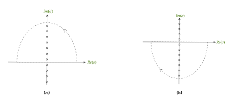
Figure 15: The contour of the integral (124)for (a) $\Delta E<0$ and (b) $\Delta E>0$.

Considering the analytic continuation of the above integrands in the complex plane of $\sigma$, for eq.(128) we get a second order pole at $\sigma=i\varepsilon$ and for eq.(129) we find a set of second order poles at $\sigma=-2i\pi k$ with $k=\pm 1,\pm 2,\ldots$, lying on the imaginary axis of $\sigma$. For $\xi<0$ or $\Delta E<0$, we close the contour in the upper half complex plane in Figure 15. Using Jordon’s lemma, we observe that the integration along the half circle is zero. Therefore, applying the Cauchy residue theorem in the integrals (128) and (129) and using it in eq.(127), we get

$$\mathcal{I}_{1}(\Delta E<0)=-\frac{\alpha}{4\pi^{2}}\Bigg{[}2\pi\xi+2\pi\xi\displaystyle\sum_{k=1}^{\infty}e^{2\pi k\xi}\Bigg{]}=\frac{\alpha|\xi|}{2\pi}\left[1+\frac{1}{e^{2\pi|\xi|}-1}\right]=\frac{|\Delta E|}{2\pi}\left[1+\frac{1}{e^{2\pi|\Delta E|/\alpha}-1}\right]\,.$$ (130)

Similarly, for $\Delta E>0$, closing the contour in the lower half complex plane and following the previous steps, we get

$$\mathcal{I}_{1}(\Delta E>0)=\frac{\Delta E}{2\pi}\frac{1}{e^{2\pi\Delta E/\alpha}-1}\,.$$ (131)

Therefore, combining the above results (130) and (131), we get

$$\mathcal{I}_{1}=\theta\,(-\Delta E)\frac{|\Delta E|}{2\pi}\left(1+\frac{1}{\exp(2\pi|\Delta E|/\alpha)-1}\right)+\theta\,(\Delta E)\frac{\Delta E}{2\pi}\left(\frac{1}{\exp(2\pi\Delta E/\alpha)-1}\right)$$ (132)

where $\theta(\Delta E)$ is the Heaviside step function.

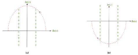
Figure 16: The contour of the integral (125) for (a) $\Delta E<0$ and (b) $\Delta E>0$.

To evaluate the integral in eq.(125), first we consider the analytic continuation of the integrand in the complex plane $\sigma$. Eq.(125) then becomes

$$\mathcal{I}_{2}=-\frac{\alpha}{16\pi^{2}}\oint_{C}d\sigma\,e^{-i\xi\sigma}\frac{1}{\sinh^{2}\left[\frac{1}{2}(\sigma-i\varepsilon)\right]-d^{2}\alpha^{2}}$$ (133)

where $C$ is the contour in Figure 16. From the integrand we find that there exists two types of first order poles $\sigma^{+}=i\varepsilon+2in\pi+2\sinh^{-1}(d\alpha)$ and $\sigma^{-}=i\varepsilon+2in\pi-2\sinh^{-1}(d\alpha)$ where $n=0,\pm 1,\pm 2,\ldots$, lying in the upper and lower half of the complex plane. Therefore, closing the contour in the upper half complex plane for $\Delta E<0$, we find that both the poles will contribute for all positive integer values of $n$ including $n=0$.
Now applying the residue theorem and taking the limit $\varepsilon\rightarrow 0$, the residues become

$$R_{1}(n)=\frac{\exp{-i\frac{\Delta E}{\alpha}(2in\pi+2\sinh^{-1}(d\alpha))}}{\alpha d\sqrt{1+d^{2}\alpha^{2}}}$$ (134)

and

$$R_{2}(n)=-\frac{\exp{-i\frac{\Delta E}{\alpha}(2in\pi-2\sinh^{-1}(d\alpha))}}{\alpha d\sqrt{1+d^{2}\alpha^{2}}}\,.$$ (135)

Applying Jordon’s lemma, we already observe that the integration along the half circle is zero, therefore we get

$$\mathcal{I}_{2}(\Delta E<0) =-\frac{\alpha}{16\pi^{2}}\displaystyle\sum_{n=0}^{\infty}2\pi i\Big{[}R_{1}(n)+R_{2}(n)\Big{]}$$

$$=\frac{\sin(\frac{2|\Delta E|}{\alpha}\sinh^{-1}(d\alpha))}{4\pi d\sqrt{1+d^{2}\alpha^{2}}}\left(1+\frac{1}{e^{2\pi|\Delta E|/\alpha}-1}\right)\,.$$ (136)

Similarly, for $\Delta E>0$, closing the contour in the lower half complex plane we find that both the poles will contribute for all negative integer values of $n$.
Now following the steps of the case $\Delta E<0$, we get

$$\mathcal{I}_{2}(\Delta E>0)=\frac{\sin(\frac{2\Delta E}{\alpha}\sinh^{-1}(d\alpha))}{4\pi d\sqrt{1+d^{2}\alpha^{2}}}\left(\frac{1}{e^{2\pi\Delta E/\alpha}-1}\right)\,.$$ (137)

Therefore, combining the above results (A) and (137), we get

$$\mathcal{I}_{2}=\theta(-\Delta E)\frac{\sin(\frac{2|\Delta E|}{\alpha}\sinh^{-1}(d\alpha))}{4\pi d\sqrt{1+d^{2}\alpha^{2}}}\left(1+\frac{1}{e^{2\pi|\Delta E|/\alpha}-1}\right)+\theta(\Delta E)\frac{\sin(\frac{2\Delta E}{\alpha}\sinh^{-1}(d\alpha))}{4\pi d\sqrt{1+d^{2}\alpha^{2}}}\left(\frac{1}{e^{2\pi\Delta E/\alpha}-1}\right)\,.$$ (138)

References

- [1] I. Fuentes-Schuller and R. B. Mann, “Alice Falls into a Black Hole: Entanglement in Noninertial Frames”, Phys. Rev. Lett. 95 (2005) 120404.
- [2] B. Richter and Y. Omar, “Degradation of entanglement between two accelerated parties: Bell states under the Unruh effect”, Phys. Rev. A 92 (2015) 022334.
- [3] P. M. Alsing, I. Fuentes-Schuller, R. B. Mann and T. E. Tessier, “Entanglement of Dirac fields in noninertial frames”, Phys. Rev. A 74 (2006) 032326.
- [4] A. Bermudez and M. A. Martin-Delgado, “Hyper-entanglement in a relativistic two-body system”, Journal of Physics A: Mathematical and Theoretical 41[48] (2008) 485302.
- [5] M.-R. Hwang, E. Jung and D. Park, “Three-tangle in non-inertial frame”, Classical and Quantum Gravity 29[22] (2012) 224004.
- [6] M.-R. Hwang, D. Park and E. Jung, “Tripartite entanglement in a noninertial frame”, Phys. Rev. A 83 (2011) 012111.
- [7] E. Hagley, X. Maître, G. Nogues, C. Wunderlich, M. Brune, J. M. Raimond and S. Haroche, “Generation of Einstein-Podolsky-Rosen Pairs of Atoms”, Phys. Rev. Lett. 79 (1997) 1.
- [8] M. B. Plenio, S. F. Huelga, A. Beige and P. L. Knight, “Cavity-loss-induced generation of entangled atoms”, Phys. Rev. A 59 (1999) 2468.
- [9] L. Amico, R. Fazio, A. Osterloh and V. Vedral, “Entanglement in many-body systems”, Rev. Mod. Phys. 80 (2008) 517.
- [10] G. S. Agarwal, “Quantum-entanglement-initiated super Raman scattering”, Phys. Rev. A 83 (2011) 023802.
- [11] B. Reznik, “Entanglement from the Vacuum”, Foundations of Physics 33[1] (2003) 167.
- [12] B. Reznik, A. Retzker and J. Silman, “Violating Bell’s inequalities in vacuum”, Phys. Rev. A 71 (2005) 042104.
- [13] D. Braun, “Entanglement from thermal blackbody radiation”, Phys. Rev. A 72 (2005) 062324.
- [14] S. Massar and P. Spindel, “Einstein-Podolsky-Rosen correlations between two uniformly accelerated oscillators”, Phys. Rev. D 74 (2006) 085031.
- [15] J. Franson, “Generation of entanglement outside of the light cone”, Journal of Modern Optics 55[13] (2008) 2117, arXiv:https://doi.org/10.1080/09500340801983129.
- [16] S.-Y. Lin and B. L. Hu, “Temporal and spatial dependence of quantum entanglement from a field theory perspective”, Phys. Rev. D 79 (2009) 085020.
- [17] S.-Y. Lin and B. L. Hu, “Entanglement creation between two causally disconnected objects”, Phys. Rev. D 81 (2010) 045019.
- [18] G. Menezes, “Radiative processes of two entangled atoms outside a Schwarzschild black hole”, Phys. Rev. D 94 (2016) 105008.
- [19] S. Sen, R. Mandal and S. Gangopadhyay, “Equivalence principle and HBAR entropy of an atom falling into a quantum corrected black hole”, Phys. Rev. D 105 (2022) 085007.
- [20] S. Sen, R. Mandal and S. Gangopadhyay, “Near horizon aspects of acceleration radiation of an atom falling into a class of static spherically symmetric black hole geometries”, Phys. Rev. D 106 (2022) 025004.
- [21] S. Sen, R. Mandal and S. Gangopadhyay, “Near horizon approximation and beyond for a two-level atom falling into a Kerr-Newman black hole”, arXiv:2301.04834 [gr-qc].
- [22] S. A. Fulling, “Nonuniqueness of Canonical Field Quantization in Riemannian Space-Time”, Phys. Rev. D 7 (1973) 2850.
- [23] P. C. W. Davies, “Scalar production in Schwarzschild and Rindler metrics”, Journal of Physics A: Mathematical and General 8[4] (1975) 609.
- [24] W. G. Unruh, “Experimental Black-Hole Evaporation?”, Phys. Rev. Lett. 46 (1981) 1351.
- [25] N. D. Birrell and P. Davies, Quantum fields in curved space, Cambridge university press 1984, URL.
- [26] V. Frolov and V. Ginzburg, “Excitation and radiation of an accelerated detector and anomalous doppler effect”, Physics Letters A 116[9] (1986) 423, URL.
- [27] A. Higuchi and G. E. A. Matsas, “Fulling-Davies-Unruh effect in classical field theory”, Phys. Rev. D 48 (1993) 689.
- [28] O. Levin, Y. Peleg and A. Peres, “Quantum detector in an accelerated cavity”, Journal of Physics A: Mathematical and General 25[23] (1992) 6471.
- [29] J. Audretsch and R. Müller, “Spontaneous excitation of an accelerated atom: The contributions of vacuum fluctuations and radiation reaction”, Phys. Rev. A 50 (1994) 1755.
- [30] J. Audretsch and R. Müller, “Radiative energy shifts of an accelerated two-level system”, Phys. Rev. A 52 (1995) 629.
- [31] R. Passante, “Radiative level shifts of an accelerated hydrogen atom and the Unruh effect in quantum electrodynamics”, Phys. Rev. A 57 (1998) 1590.
- [32] D. A. T. Vanzella and G. E. A. Matsas, “Decay of Accelerated Protons and the Existence of the Fulling-Davies-Unruh Effect”, Phys. Rev. Lett. 87 (2001) 151301.
- [33] D. T. Alves and L. C. B. Crispino, “Response rate of a uniformly accelerated source in the presence of boundaries”, Phys. Rev. D 70 (2004) 107703.
- [34] H. Yu and S. Lu, “Spontaneous excitation of an accelerated atom in a spacetime with a reflecting plane boundary”, Phys. Rev. D 72 (2005) 064022.
- [35] Z. Zhu, H. Yu and S. Lu, “Spontaneous excitation of an accelerated hydrogen atom coupled with electromagnetic vacuum fluctuations”, Phys. Rev. D 73 (2006) 107501.
- [36] H. Yu and Z. Zhu, “Spontaneous absorption of an accelerated hydrogen atom near a conducting plane in vacuum”, Phys. Rev. D 74 (2006) 044032.
- [37] S.-Y. Lin and B. L. Hu, “Accelerated detector-quantum field correlations: From vacuum fluctuations to radiation flux”, Phys. Rev. D 73 (2006) 124018.
- [38] Z. Zhu and H. Yu, “Fulling–Davies–Unruh effect and spontaneous excitation of an accelerated atom interacting with a quantum scalar field”, Physics Letters B 645[5] (2007) 459, URL.
- [39] W. Zhou and H. Yu, “Spontaneous excitation of a uniformly accelerated atom coupled to vacuum Dirac field fluctuations”, Phys. Rev. A 86 (2012) 033841.
- [40] Z. Zhi-Ying and Y. Hong-Wei, “Accelerated Multi-Level Atoms in an Electromagnetic Vacuum and Fulling–Davies–Unruh Effect”, Chinese Physics Letters 25[5] (2008) 1575.
- [41] L. C. B. Crispino, A. Higuchi and G. E. A. Matsas, “Interaction of Hawking radiation and a static electric charge”, Phys. Rev. D 58 (1998) 084027.
- [42] D. Marolf, D. Minic and S. F. Ross, “Notes on spacetime thermodynamics and the observer dependence of entropy”, Phys. Rev. D 69 (2004) 064006.
- [43] G. E. A. Matsas and A. R. R. da Silva, “New thought experiment to test the generalized second law of thermodynamics”, Phys. Rev. D 71 (2005) 107501.
- [44] A. Noto and R. Passante, “van der Waals interaction energy between two atoms moving with uniform acceleration”, Phys. Rev. D 88 (2013) 025041.
- [45] J. Marino, A. Noto and R. Passante, “Thermal and Nonthermal Signatures of the Unruh Effect in Casimir-Polder Forces”, Phys. Rev. Lett. 113 (2014) 020403.
- [46] L. Rizzuto, M. Lattuca, J. Marino, A. Noto, S. Spagnolo, W. Zhou and R. Passante, “Nonthermal effects of acceleration in the resonance interaction between two uniformly accelerated atoms”, Phys. Rev. A 94 (2016) 012121.
- [47] W. Zhou, R. Passante and L. Rizzuto, “Resonance interaction energy between two accelerated identical atoms in a coaccelerated frame and the Unruh effect”, Phys. Rev. D 94 (2016) 105025.
- [48] G. Fiscelli, L. Rizzuto and R. Passante, “Resonance energy transfer between two atoms in a conducting cylindrical waveguide”, Phys. Rev. A 98 (2018) 013849.
- [49] G. Menezes and N. F. Svaiter, “Radiative processes of uniformly accelerated entangled atoms”, Phys. Rev. A 93 (2016) 052117.
- [50] M. S. Soares, N. F. Svaiter, C. A. D. Zarro and G. Menezes, “Uniformly accelerated quantum counting detector in Minkowski and Fulling vacuum states”, Phys. Rev. A 103 (2021) 042225.
- [51] W. Zhou, L. Rizzuto and R. Passante, “Vacuum fluctuations and radiation reaction contributions to the resonance dipole-dipole interaction between two atoms near a reflecting boundary”, Phys. Rev. A 97 (2018) 042503.
- [52] C. A. U. Lima, F. Brito, J. A. Hoyos and D. A. T. Vanzella, “Probing the Unruh effect with an accelerated extended system”, Nature Communications 10[1] (2019) 3030.
- [53] J. D. Thompson, T. G. Tiecke, N. P. de Leon, J. Feist, A. V. Akimov, M. Gullans, A. S. Zibrov, V. Vuletić and M. D. Lukin, “Coupling a Single Trapped Atom to a Nanoscale Optical Cavity”, Science 340[6137] (2013) 1202.
- [54] P. Solano, J. A. Grover, J. E. Hoffman, S. Ravets, F. K. Fatemi, L. A. Orozco and S. L. Rolston, “Chapter Seven - Optical Nanofibers: A New Platform for Quantum Optics”, p. 439–505, Academic Press 2017, URL.
- [55] E. Vetsch, D. Reitz, G. Sagué, R. Schmidt, S. T. Dawkins and A. Rauschenbeutel, “Optical Interface Created by Laser-Cooled Atoms Trapped in the Evanescent Field Surrounding an Optical Nanofiber”, Phys. Rev. Lett. 104 (2010) 203603.
- [56] A. Goban, K. S. Choi, D. J. Alton, D. Ding, C. Lacroûte, M. Pototschnig, T. Thiele, N. P. Stern and H. J. Kimble, “Demonstration of a State-Insensitive, Compensated Nanofiber Trap”, Phys. Rev. Lett. 109 (2012) 033603.
- [57] N. V. Corzo, J. Raskop, A. Chandra, A. S. Sheremet, B. Gouraud and J. Laurat, “Waveguide-coupled single collective excitation of atomic arrays”, Nature 566[7744] (2019) 359, URL.
- [58] D. E. Chang, J. S. Douglas, A. González-Tudela, C.-L. Hung and H. J. Kimble, “Colloquium: Quantum matter built from nanoscopic lattices of atoms and photons”, Rev. Mod. Phys. 90 (2018) 031002.
- [59] N. Friis, A. R. Lee, K. Truong, C. Sabín, E. Solano, G. Johansson and I. Fuentes, “Relativistic Quantum Teleportation with Superconducting Circuits”, Phys. Rev. Lett. 110 (2013) 113602.
- [60] S. Felicetti, C. Sabín, I. Fuentes, L. Lamata, G. Romero and E. Solano, “Relativistic motion with superconducting qubits”, Phys. Rev. B 92 (2015) 064501.
- [61] Z. Huang and H. Situ, “Protection of quantum dialogue affected by quantum field”, Quantum Information Processing 18[1].
- [62] Z. Huang and Z. He, “Deterministic secure quantum communication under vacuum fluctuation”, The European Physical Journal D 74[9].
- [63] M. R. R. Good, A. Lapponi, O. Luongo and S. Mancini, “Quantum communication through a partially reflecting accelerating mirror”, Phys. Rev. D 104 (2021) 105020.
- [64] J. Åberg, S. Hengl and R. Renner, “Directed quantum communication”, New Journal of Physics 15[3] (2013) 033025.
- [65] J. Zhang and H. Yu, “Unruh effect and entanglement generation for accelerated atoms near a reflecting boundary”, Phys. Rev. D 75 (2007) 104014.
- [66] R. Zhou, R. O. Behunin, S.-Y. Lin and B. Hu, “Boundary effects on quantum entanglement and its dynamics in a detector-field system”, Journal of High Energy Physics 2013[8].
- [67] S. Cheng, H. Yu and J. Hu, “Entanglement dynamics for uniformly accelerated two-level atoms in the presence of a reflecting boundary”, Phys. Rev. D 98 (2018) 025001.
- [68] Z. Liu, J. Zhang and H. Yu, “Entanglement harvesting in the presence of a reflecting boundary”, Journal of High Energy Physics 2021[8].
- [69] I. Akal, Y. Kusuki, N. Shiba, T. Takayanagi and Z. Wei, “Holographic moving mirrors”, Classical and Quantum Gravity 38[22] (2021) 224001.
- [70] R. Chatterjee, S. Gangopadhyay and A. S. Majumdar, “Resonance interaction of two entangled atoms accelerating between two mirrors”, Eur. Phys. J. D 75[6] (2021) 179.
- [71] A. Mukherjee, S. Gangopadhyay and A. S. Majumdar, “Unruh quantum Otto engine in the presence of a reflecting boundary”, Journal of High Energy Physics 2022[9] (2022) 105.
- [72] S. Haroche and J.-M. Raimond, Exploring the quantum: atoms, cavities, and photons, Oxford university press 2006, URL.
- [73] R. Chatterjee, S. Gangopadhyay and A. S. Majumdar, “Violation of equivalence in an accelerating atom-mirror system in the generalized uncertainty principle framework”, Phys. Rev. D 104 (2021) 124001.
- [74] M. O. Scully, V. V. Kocharovsky, A. Belyanin, E. Fry and F. Capasso, “Enhancing Acceleration Radiation from Ground-State Atoms via Cavity Quantum Electrodynamics”, Phys. Rev. Lett. 91 (2003) 243004.
- [75] A. Belyanin, V. V. Kocharovsky, F. Capasso, E. Fry, M. S. Zubairy and M. O. Scully, “Quantum electrodynamics of accelerated atoms in free space and in cavities”, Phys. Rev. A 74 (2006) 023807.
- [76] G. A. Mourou, T. Tajima and S. V. Bulanov, “Optics in the relativistic regime”, Rev. Mod. Phys. 78 (2006) 309.
- [77] U. Eichmann, T. Nubbemeyer, H. Rottke and W. Sandner, “Acceleration of neutral atoms in strong short-pulse laser fields”, Nature 461[7268] (2009) 1261.
- [78] C. Maher-McWilliams, P. Douglas and P. F. Barker, “Laser-driven acceleration of neutral particles”, Nature Photonics 6[6] (2012) 386.
- [79] E. Arias, J. Dueñas, G. Menezes and N. Svaiter, “Boundary effects on radiative processes of two entangled atoms”, Journal of High Energy Physics 2016[7].
- [80] C. Zhang and W. Zhou, “Radiative Processes of Two Accelerated Entangled Atoms Near Boundaries”, Symmetry 11[12], URL.
- [81] W. Zhou and H. Yu, “Collective transitions of two entangled atoms and the Fulling-Davies-Unruh effect”, Phys. Rev. D 101 (2020) 085009.
- [82] K. Lochan, H. Ulbricht, A. Vinante and S. K. Goyal, “Detecting Acceleration-Enhanced Vacuum Fluctuations with Atoms Inside a Cavity”, Phys. Rev. Lett. 125 (2020) 241301.
- [83] D. J. Stargen and K. Lochan, “Cavity Optimization for Unruh Effect at Small Accelerations”, Phys. Rev. Lett. 129 (2022) 111303.
- [84] N. Arya, V. Mittal, K. Lochan and S. K. Goyal, “Geometric phase assisted observation of noninertial cavity-QED effects”, Phys. Rev. D 106 (2022) 045011.
- [85] B. F. Svaiter and N. F. Svaiter, “Inertial and noninertial particle detectors and vacuum fluctuations”, Phys. Rev. D 46 (1992) 5267.
- [86] M. E. Peskin, An introduction to quantum field theory, CRC press 2018.
- [87] E. Freitag and R. Busam, Complex Analysis, Universitext, Springer Berlin Heidelberg 2009.
- [88] J. E. Sansonetti, “Wavelengths, Transition Probabilities, and Energy Levels for the Spectra of Rubidium”, Journal of Physical and Chemical Reference Data 35[1] (2006) 301.
- [89] C. Rodríguez-Camargo, G. Menezes and N. Svaiter, “Finite-time response function of uniformly accelerated entangled atoms”, Annals of Physics 396 (2018) 266, URL.
- [90] M. Donaire, J. M. Muñoz Castañeda and L. M. Nieto, “Dipole-dipole interaction in cavity QED: The weak-coupling, nondegenerate regime”, Phys. Rev. A 96 (2017) 042714.
- [91] I. S. Gradshteyn, I. M. Ryzhik, D. Zwillinger and V. Moll, Table of integrals, series, and products; 8th ed., Academic Press, Amsterdam 2014, URL.