Exact Spatio-Temporal Dynamics of Lattice Random Walks in Hexagonal and Honeycomb Domains

Abstract

A variety of transport processes in natural and man-made systems are intrinsically random. To model their stochasticity, lattice random walks have been employed for a long time, mainly by considering Cartesian lattices. However, in many applications in bounded space the geometry of the domain may have profound effects on the dynamics and ought to be accounted for. We consider here the cases of the six-neighbour (hexagonal) and three-neighbour (honeycomb) lattice, which are utilised in models ranging from adatoms diffusing in metals and excitations diffusing on single-walled carbon nanotubes to animal foraging strategy and the formation of territories in scent-marking organisms. In these and other examples, the main theoretical tool to study the dynamics of lattice random walks in hexagonal geometries has been via simulations. Analytic representations have in most cases been inaccessible, in particular in bounded hexagons, given the complicated ‘zig-zag’ boundary conditions that a walker is subject to. Here we generalise the method of images to hexagonal geometries and obtain closed-form expressions for the occupation probability, the so-called propagator, for lattice random walks both on hexagonal and honeycomb lattices with periodic, reflective and absorbing boundary conditions. In the periodic case, we identify two possible choices of image placement and their corresponding propagators. Using them, we construct the exact propagators for the other boundary conditions, and we derive transport related statistical quantities such as first passage probabilities to one or multiple targets and their means, elucidating the effect of the boundary condition on transport properties.

I Introduction

Popularised in the 1920s by Pólya [1], lattice random walks (LRW) are widely used in the mathematics [2] and physics [3, 4, 5] literature. Owing to their versatility as a special class of Markov chains, one finds applications of LRW across a multitude of disciplines including animal ecology [6, 7], cell biology [8], actuarial science [9] and social sciences [10]. While analytic representations of the dynamics of LRW has been studied for a long time, recent advances in the exact description of their dynamics in finite $d$-dimensional hypercubic lattices [11, 12, 13, 14] have brought renewed interest. Following these advances, many computationally challenging problems such as transmission and encounter dynamics between LRW pairs [15] and the dynamics of interactions with inert spatial heterogeneities can now be tackled analytically [16].

These developments are, however, limited to Cartesian lattices with little attention given to other geometries. In $d=2$ dimensions, two such important cases are the hexagonal and the honeycomb lattices, often found to be used interchangeably in the literature [17, 18, 19]. To avoid any confusion, in the present work we refer to a hexagonal lattice when each site has six nearest-neigbours and to a honeycomb lattice when each site has three nearest-neighbours.

Random walks on both lattices have been employed to study many stochastic processes. The hexagonal lattice has been used to represent adatom diffusion in metals [20], space usage and foraging of animals [21], territory formation in scent-marking organisms [22, 23], and substrate diffusion across artificial tissue [24], while the honeycomb LRW has been utilised for particle movement in ice and graphite [25] and the diffusion of excitons on a single-walled carbon nanotube (SWCN) [26, 27]. Both lattices are also of interest in the context of self-avoiding walks [28, 29].

For both lattices, when unbounded, the walk statistics have been studied by mapping the dynamics onto a square lattice. To model a hexagonal walk, two of the eight permissible movement directions in a next nearest-neighbour walk are removed [19, 30], while a brick-like structure of positive and negative sites is created to represent the honeycomb LRW [4, 31]. Another approach, applicable to the honeycomb lattice, models the domain as a bipartite network allowing the construction of the propagator generating function for an unbounded walker that always moves [18].

For many of the applications stated earlier, the movement statistics are heavily affected by the size of the underlying spatial domain. In the literature, analytical attempts to take into consideration the finiteness of the space have been rare, largely due to the non-orthogonal configuration of lattice sites, which leads to complex ‘zig-zag’ boundaries. One example, which aims to account for the dynamics at the boundary, considers a four walled domain with two opposing walls made up of absorbing sites and the other two walls representing a periodic domain. Via the use of a technique to solve inhomogenous linear partial difference equations [32], analytic expressions for the expectation value that the walk reaches a lattice site before getting absorbed have been obtained [33].

To represent faithfully the finiteness of the hexagonal space, we introduce here a framework for the analytic representation of the spatio-temporal dynamics of LRW in hexagonal geometries with true ‘zig-zag’ boundaries. We utilise a non-orthogonal hexagonal coordinate system [34, 35] for both lattices and model the honeycomb lattice via the inclusion of internal states [36, 4]. By deriving an extension of the method of images [37] to hexagonal space we find closed-form expressions for the propagator, in periodically bounded random walks. We generalise the defect technique [38, 15, 16] to hexagonal space and random walks with internal states and obtain analytically the propagator generating function for both LRW with absorbing and reflecting boundary conditions. Various transport properties in both lattices are also analysed.

The outline of the paper is as follows. In Sec. II we introduce the coordinate system used to parameterise the lattices. Section III is devoted to the analysis of the unbounded lattice Green’s function or propagator for both the hexagonal and honeycomb random walk. In Sec. IV, closed-form expressions for the propagator, in two representations of periodically bounded domains are obtained. In Secs. V and VI, we derive the propagators for absorbing and reflecting domains, respectively. Transport properties are studied in Sec. VII where we present the analytic representation of the first passage probability, or first-hitting time, to a target, while in Sec. VIII we derive closed-from expressions for the mean first passage time to one target and employ it to study the mean first passage to multiple targets.

II Hexagonal Coordinate System

A convenient coordinate system for hexagonal lattices, designed for application in computer graphics [34, 35], is given by three linearly dependent integer coordinates $(n_{1},n_{2},n_{3})$ such that $n_{1}+n_{2}+n_{3}=0$. One can represent these coordinates on two different axis sets: an oblique plane in $\mathbb{R}^{3}$ or three axes lying 60 degrees apart in $\mathbb{R}^{2}$. We take the latter, whose visual representation can be found in Fig. 1(a), and we refer to the coordinate system as hexagonal cubic coordinates (HCC). The HCC system is related to $\mathbb{R}^{2}$ Cartesian coordinates $(x_{1},x_{2})$ via the transformation [39]

$$n_{1}=-\frac{x_{2}}{2}+\frac{\sqrt{3}x_{1}}{2};\;\>\;n_{2}=x_{2};\;\>\;n_{3}=-\frac{x_{2}}{2}-\frac{\sqrt{3}x_{1}}{2},$$ (1)

where $n_{1},n_{2},n_{3}\in\mathbb{Z}$ and $x_{1},x_{2}\in\mathbb{R}$, which enables convenient plotting.

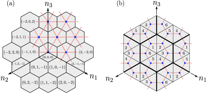
Figure 1: (Colour online). A schematic representation of the hexagonal lattice, panel (a), and the honeycomb lattice, panel (b). In (a), we show the HCC in $\mathbb{R}^{2}$ with three non-orthogonal axes. Coordinate labels are shown on some lattice sites, while permissible movement directions for the hexagonal lattice are shown on others with dotted lines. For clarity, we omit arrows depicting the option of staying on lattice sites. In (b) we show the honeycomb lattice. Here we show the $(0,0,0)$ Wigner-Seitz cell, half of its six neighbours and their labelled internal states. Permissible movement directions are again shown through dotted lines and similarly to panel (a), arrows representing the option of remaining on any site are removed. The boundaries of the hexagonal Wigner-Seitz cell are shown in bolder lines.

II.1 Finite Hexagonal Lattice

We model permissible jumps to neighbouring sites taking place between the centroid of the so-called Wigner-Seitz cell (WS) and its six neighbours, shown in Fig. 1(a), giving a coordination number $Z=6$. We also allow for the option of remaining on the lattice site at each timestep. The size of the finite domain is controlled by the single parameter $R$, the circumradius of the hexagon. The corners lie at $(n_{1},n_{2},n_{3})=(\pm R,0,\mp R)$, $(n_{1},n_{2},n_{3})=(\pm R,\mp R,0)$, and $(n_{1},n_{2},n_{3})=(0,\pm R,\mp R)$.

II.2 Finite Honeycomb Lattice

The honeycomb lattice has a coordination number $Z=3$ and each lattice site can be thought of as a vertex of the hexagonal WS cell, making the honeycomb lattice the dual of the hexagonal lattice [40]. We model this lattice as a tessellation of even ($\rhd$) and odd ($\lhd$) triangles by utilising the HCC and including internal states. To avoid confusion, we refer to the hexagonal WS cell, with coordinates $(n_{1},n_{2},n_{3})$ as a lattice site, which contains six internal states labelled $m_{i}$, $i=\{1,...6\}$ starting from the top left triangle and going clockwise round the unit cell, shown in Fig. 1(b). At each timestep the walker has four permissible actions: to remain on the same lattice site and state, to move to either of two adjacent states in the same site or to move to an adjacent state in an adjacent site. The number of locations the walker can reach in the honeycomb lattice is six times bigger than in the hexagonal lattice with the same circumradius.

III Dynamics in Unbounded Space

With later sections exploiting the analytic representation of the occupation probability for the infinite lattice to construct bounded propagators, we show here the procedure to obtain the unbounded case.

III.1 Hexagonal Lattice

The Master equation governing the evolution of the site occupation probability, $Q(n_{1},n_{2},n_{3},t)$, for the unbounded hexagonal lattice is represented by

$$Q( n_{1},n_{2},n_{3},t+1)=\frac{q}{6}\bigg{[}Q(n_{1}-1,n_{2},n_{3}+1,t)+Q(n_{1},n_{2}-1,n_{3}+1,t)+Q(n_{1}+1,n_{2}-1,n_{3},t)$$ (2)

$$+Q(n_{1}+1,n_{2},n_{3}-1,t)+Q(n_{1},n_{2}+1,n_{3}-1,t)+Q(n_{1}-1,n_{2}+1,n_{3},t)\bigg{]}+(1-q)Q(n_{1},n_{2},n_{3},t),$$

where $q$ ($0<q\leq 1$), determines the probability of movement, that is $q=1$ represents a walker changing lattice site at every timestep. Eq. (2) is subject to the initial condition $Q(n_{1},n_{2},n_{3},0)=\delta_{n_{{}_{1}}n_{0_{1}}}\delta_{n_{{}_{2}}n_{0_{2}}}\delta_{n_{{}_{3}}n_{0_{3}}}$, where $\delta_{ij}$ is the Kronecker delta and $n_{0_{1}}+n_{0_{2}}+n_{0_{3}}=0$.

While Eq. (2) is well suited for the infinite lattice, in the bounded cases the linear relationship between the coordinates, $n_{3}=-n_{1}-n_{2}$, makes it necessary (see Appendix B) to drop the $n_{3}$ dependence and re-write the Master equation with a two coordinate representation given by

$$Q( n_{1},n_{2},t+1)=\frac{q}{6}\bigg{[}Q(n_{1}-1,n_{2},t)+Q(n_{1},n_{2}-1,t)+Q(n_{1}+1,n_{2}-1,t)+$$ (3)

$$Q(n_{1}+1,n_{2},t)+Q(n_{1},n_{2}+1,t)+Q(n_{1}-1,n_{2}+1,t)\bigg{]}+(1-q)Q(n_{1},n_{2},t).$$

After applying the discrete Fourier transform $\widehat{f}(k)=\sum_{n=-\infty}^{\infty}e^{-ikn}f(n)$ and the unilateral $z$-transform $\widetilde{f}(z)=\sum_{t=0}^{\infty}z^{t}f(t)$, we solve Eq. (3) to obtain the hexagonal lattice Green’s function as a double integral

$$\widetilde{Q}_{\bm{n}_{0}}(n_{1},n_{2},z)=\frac{1}{(2\pi)^{2}}\int_{-\pi}^{\pi}\int_{-\pi}^{\pi}\frac{e^{i[(\bm{n}-\bm{n}_{0})\cdot\bm{k}]}}{1-z\mu(k_{1},k_{2})}dk_{1}dk_{2},$$ (4)

where $\bm{k}=(k_{1},k_{2})^{\intercal}$ and $\bm{n}-\bm{n}_{0}=(n_{{}_{1}}-n_{0_{1}},n_{{}_{2}}-n_{0_{2}})$ and $\mu(k_{1},k_{2})=1-q+\frac{q}{3}\left[\cos(k_{1}-k_{2})+\cos(k_{1})+\cos(k_{2})\right]$ is the so-called structure function, or discrete Fourier transform of the individual step probabilities [3]. Equation (4) reduces to known results when $q=1$ [19].

III.2 Honeycomb Lattice

The general form of the Master equation for a LRW with internal states has the vectorial form [41, 4]

$$\bm{\mathcal{Q}}(\bm{n},t+1)=\sum_{\bm{n}^{\prime}}\mathbb{W}(\bm{n},\bm{n}^{\prime})\bm{\mathcal{Q}(\bm{n}^{\prime}},t),$$ (5)

where $\mathbb{W}(\bm{n},\bm{n}^{\prime})$ represents all possible movement from $\bm{n}^{\prime}$ to site $\bm{n}$ at each moment in time and $\bm{\mathcal{Q}(\bm{n}^{\prime}},t)$ is a column vector representing the occupation probability of each internal state in site $\bm{n}^{\prime}$ at time $t$. For the honeycomb lattice, Eq. (5) reduces to

$$\bm{\mathcal{Q}}( n_{1},n_{2},t+1)=\frac{q}{3}\bigg{[}\mathbb{A}_{1,4}\cdot\bm{\mathcal{Q}}(n_{1}-1,n_{2},t)+\mathbb{A}_{2,5}\cdot\bm{\mathcal{Q}}(n_{1},n_{2}-1,t)+\mathbb{A}_{3,6}\cdot\bm{\mathcal{Q}}(n_{1}+1,n_{2}-1,t)+$$ (6)

$$\mathbb{A}_{4,1}\cdot\bm{\mathcal{Q}}(n_{1}+1,n_{2},t)+\mathbb{A}_{5,2}\cdot\bm{\mathcal{Q}}(n_{1},n_{2}+1,t)+\mathbb{A}_{6,3}\cdot\bm{\mathcal{Q}}(n_{1}-1,n_{2}+1,t)\bigg{]}+\mathbb{B}\cdot\bm{\mathcal{Q}}(n_{1},n_{2},t),$$

where $\mathbb{A}_{i,j}$ is a $6\times 6$ matrix with value one at index $i,j$ that represents the movement from state $i$ in one WS cell to state $j$ in a new WS cell, as depicted in Fig. 1(b). $\mathbb{B}$, which represents the movement within one WS cell, is a tridiagonal Toeplitz matrix with perturbed corners where $\mathbb{B}_{i,i}=1-q$ with $i\leq 1\leq 6$, $\mathbb{B}_{i+1,i}=\mathbb{B}_{i,i+1}=\frac{q}{3}$ with $1\leq i\leq 5$, $\mathbb{B}_{1,6}=\mathbb{B}_{6,1}=\frac{q}{3}$ and zero elsewhere.

Taking the localised initial condition $\bm{\mathcal{Q}}(n_{1},n_{2},t=0)=\delta_{\bm{n}\bm{n}_{0}}\bm{U}_{m_{0}}$, where $\bm{U}_{m_{0}}$ is a $6\times 1$ column vector with element $m_{0}$ exactly one and the rest exactly zero, and following standard techniques for random walks with internal states (see e.g. [4]), we obtain the generating function of the unbounded propagator

$$\widetilde{\bm{\mathcal{Q}}}_{\bm{n}_{0},m_{0}}(n_{1},n_{2},z)=\frac{1}{(2\pi)^{2}}\int_{-\pi}^{\pi}\int_{-\pi}^{\pi}e^{i[(\bm{n}-\bm{n}_{0})\cdot\bm{k}]}\left[\mathbb{I}-z\bm{\mu}(k_{1},k_{2})\right]^{-1}\cdot\bm{U}_{m_{0}}dk_{1}dk_{2},$$ (7)

where $\mathbb{I}$ is the $6\times 6$ identity matrix and the structure function

$$\bm{\mu}(k_{1},k_{2})=$$ (8)

$$\begin{bmatrix}1-q&\frac{q}{3}&0&\frac{q}{3}e^{-ik_{1}}&0&\frac{q}{3}\\ \frac{q}{3}&1-q&\frac{q}{3}&0&\frac{q}{3}e^{-ik_{2}}&0\\ 0&\frac{q}{3}&1-q&\frac{q}{3}&0&\frac{q}{3}e^{i(k_{1}-k_{2})}\\ \frac{q}{3}e^{ik_{1}}&0&\frac{q}{3}&1-q&\frac{q}{3}&0\\ 0&\frac{q}{3}e^{ik_{2}}&0&\frac{q}{3}&1-q&\frac{q}{3}\\ \frac{q}{3}&0&\frac{q}{3}e^{-i(k_{1}-k_{2})}&0&\frac{q}{3}&1-q\\ \end{bmatrix}.$$

To access the probability at a unique state $m$ one simply takes the scalar dot product $\widetilde{\mathcal{Q}}_{\bm{n}_{0},m_{0}}(n_{1},n_{2},m,z)=\bm{U}_{m}^{\intercal}\cdot\widetilde{\bm{\mathcal{Q}}}_{\bm{n}_{0},m_{0}}(n_{1},n_{2},z)$.

IV Periodic Boundary Conditions

To impose periodic boundary conditions, we generalise the method of images [37] to hexagonal domains. The technique represents a convenient way to impose boundary conditions on Green’s functions. To implement the technique for fully bounded domains, one considers an infinite set of initial conditions, tessellated across the space, which act concurrently by mirroring the walker’s movement. To tessellate hexagonal lattices in 2-dimensional space, there are two choices for the placement of the neighbouring domains due to the ‘zig-zag’ nature of the boundaries, which differ depending on whether the images are located with a so-called left or right shift in relation to one of the axes. To illustrate, let us consider the hexagon directly above the chosen finite domain. If the bottom right corner of the neighbouring domain is to the right of the top right corner of the modelled domain, it is referred to as the right shift tessellation, otherwise, it is to the left, and is referred to as the left shift tessellation (see Appendix A for a pictorial representation).

Using either tessellation, we construct an infinite number of images of the initial condition and obtain the bounded periodic propagator

$$\widetilde{P}^{(p)}_{\bm{n}_{0}}(n_{1},n_{2},z)=\sum_{m_{1}=-\infty}^{\infty}\sum_{m_{2}=-\infty}^{\infty}\widetilde{Q}_{\bm{n}_{0}}(n_{1}+\hat{n}_{1},n_{2}+\hat{n}_{2},z),$$ (9)

built by considering the appropriate coordinate transform from a location in the finite hexagonal domain to the equivalent location in any of the infinite neighbouring domains. For the right shift we find

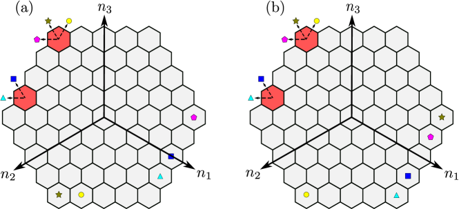
Figure 2: (Colour online). A schematic showing the difference in boundary dynamics for two specific lattice sites between the left shift, panel (a), and the right shift, panel (b). The dashed arrows show permissible directions of movement at the two chosen boundary sites and the shape at the end of the arrow corresponds with the shape indicating where this direction of travel would lead to.

$$\begin{bmatrix}\widehat{n}_{1}\\ \widehat{n}_{2}\end{bmatrix}=\begin{bmatrix}-Rm_{1}+(2R+1)m_{2}\\ -(R+1)m_{1}-Rm_{2}\end{bmatrix},$$ (10)

and for the left shift

$$\begin{bmatrix}\widehat{n}_{1}\\ \widehat{n}_{2}\end{bmatrix}=\begin{bmatrix}(2R+1)m_{1}-Rm_{2}\\ -(R+1)m_{1}+(2R+1)m_{2}\end{bmatrix},$$ (11)

where $m_{1},m_{2}\in\mathbb{Z}$.

IV.1 Hexagonal Lattice

Applying Eq. (4) in Eq. (9) and interchanging the order of integration and summation, as is permissible in generalised function theory [4], one solves (see Appendix B) for the periodic propagator

$$P_{\bm{n}_{0}}^{(p)_{[i]}}(n_{1},n_{2}, t)=\frac{1}{\Omega}+\frac{2}{\Omega}\sum_{r=0}^{R-1}\sum_{s=0}^{3r+2}\cos\left(\frac{2\pi\left[k_{1}^{[i]}(r,s)\left(n_{1}-n_{0_{1}}\right)+k_{2}^{[i]}(r,s)\left(n_{2}-n_{0_{2}}\right)\right]}{\Omega}\right)$$ (12)

$$\times\left(1-q+\frac{q}{3}\left[\cos\left(\frac{2\pi\left(k_{1}^{[i]}(r,s)-k_{2}^{[i]}(r,s)\right)}{\Omega}\right)+\cos\left(\frac{2\pi k_{1}^{[i]}(r,s)}{\Omega}\right)+\cos\left(\frac{2\pi k_{2}^{[i]}(r,s)}{\Omega}\right)\right]\right)^{t},$$

with $i\in\{\rho,\lambda\}$ indicating the right and left shift respectively. $\Omega$ is the number of lattice sites in the finite domain, namely $\Omega=3R^{2}+3R+1$, and

$$k^{[\rho]}_{1}(r,s) =k^{[\lambda]}_{2}(r,s)=R(s+1)+s-r,$$ (13)

$$k^{[\rho]}_{2}(r,s) =k^{[\lambda]}_{1}(r,s)=R(2-s+3r)+r+1.$$

We note here that as $k_{1}(r,s)$ and $k_{2}(r,s)$ are interchanged under the transition between $\rho$ and $\lambda$, the structure function is not dependent on this choice. We further note that one can also find $\Omega$ using the so-called centered hexagonal number [42, 22].

While the dynamics in the bulk are identical, the walker acts differently at the boundaries depending on the chosen shift (see Fig. 2). As we will see in Secs. VII and VIII, it may lead to marked differences in the first passage probability and mean first passage (MFPT) time.

We note that Eq. (12) is still valid for the trivial $R=0$ case where the domain reduces to a single point at the origin. Here, the two summations disappear and the solution reduces to $P_{\bm{n}_{0}}^{(p)_{[i]}}(n_{1},n_{2},t)=\frac{1}{\Omega}=1$, irrespective of the shift, as expected.

IV.2 Honeycomb Lattice

Since the honeycomb lattice is created by considering the hexagonal lattice with internal states, the set of images used to construct the finite hexagonal propagator in Sec. IV can also be applied to the honeycomb case. Using Eq. (7) in the $6\times 1$ column vectorial equivalent of Eq. (9), the periodically bounded honeycomb LRW propagator is given by (Appendix C)

$$\bm{\mathcal{P}}^{(p)_{[i]}}_{\bm{n}_{0},m_{0}}(n_{1},n_{2},t)=\frac{\bm{\mu}(0,0)^{t}\cdot\bm{U}_{m_{0}}}{\Omega} +\frac{1}{\Omega}\sum_{r=0}^{R-1}\sum_{s=0}^{3r+2}\Bigg{\{}e^{\frac{2\pi i(\bm{n}-\bm{n}_{0})\cdot\bm{k}^{[i]}(r,s)}{\Omega}}\bm{\mu}\left(\frac{2\pi k_{1}^{[i]}(r,s)}{\Omega},\frac{2\pi k_{2}^{[i]}(r,s)}{\Omega}\right)^{t}$$ (14)

$$+e^{\frac{-2\pi i(\bm{n}-\bm{n}_{0})\cdot\bm{k}^{[i]}(r,s)}{\Omega}}\bm{\mu}\left(\frac{-2\pi k_{1}^{[i]}(r,s)}{\Omega},\frac{-2\pi k_{2}^{[i]}(r,s)}{\Omega}\right)^{t}\Bigg{\}}\cdot\bm{U}_{m_{0}},$$

where $k^{[i]}_{1}(r,s),k^{[i]}_{2}(r,s)$ are defined in Eq. (13). To lighten the notation, from here onwards we drop the explicit $(r,s)$ dependence on $k^{[i]}_{1}(r,s),k^{[i]}_{2}(r,s)$.

To obtain $\mathcal{P}^{(p)_{[i]}}_{\bm{n}_{0},m_{0}}(n_{1},n_{2},m,t)$ a scalar dot product is taken, i.e. $\mathcal{P}^{(p)_{[i]}}_{\bm{n}_{0},m_{0}}(n_{1},n_{2},m,t)=\bm{U}_{m}^{\intercal}\cdot\bm{\mathcal{P}}^{(p)_{[i]}}_{\bm{n}_{0},m_{0}}(n_{1},n_{2},t)$. When $R=0$, one is left with six internal states at the origin and Eq. (14) reduces to the dynamics dictated by its first term.

For $0<q<1$, as $t\to\infty$, $\bm{\mu}\left(\frac{2\pi k_{1}^{[i]}}{\Omega},\frac{2\pi k_{2}^{[i]}}{\Omega}\right)^{t}$, $\bm{\mu}\left(\frac{-2\pi k_{1}^{[i]}}{\Omega},\frac{-2\pi k_{2}^{[i]}}{\Omega}\right)^{t}\to\bm{0}$, while $\bm{\mu}\left(0,0\right)^{t}\to\frac{1}{6}\mathbb{J}$, where $\mathbb{J}$ is an all-ones matrix (see Appendix C.1), leaving the steady state probability as $\mathcal{P}_{\bm{n}_{0},m_{0}}^{(p)_{[i]}}(n_{1},n_{2},m,t=\infty)=\frac{1}{6\Omega}$. Note that due to the odd coordination number, parity issues appear when $q=1$. That is, if the walker starts on an even (odd) site number, for large even $t$ the steady state probability on odd (even) sites $\mathcal{P}_{\bm{n}_{0},m_{0}}^{(p)_{[i]}}(n_{1},n_{2},m,t=\infty)=0$, while on even (odd) sites, $\mathcal{P}_{\bm{n}_{0},m_{0}}^{(p)_{[i]}}(n_{1},n_{2},m,t=\infty)=\frac{1}{3\Omega}$. This can again be seen by studying $\bm{\mu}\left(0,0\right)$ (Appendix C.1).

Note also that the term inside the double summation of Eq. (14) is the addition between a matrix and its Hermitian transpose, which ensures the propagator gives real values. We illustrate this by plotting, from Eq. (14), the occupation probability after two separate timesteps in Fig. 3.

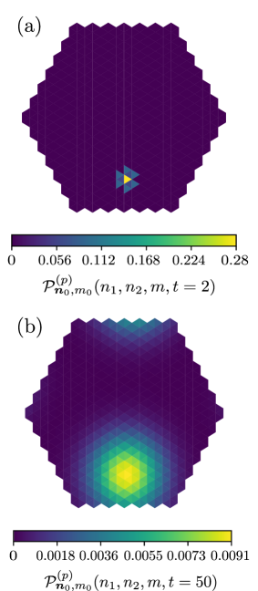
Figure 3: (Colour online). The occupation probability of the right shift bounded periodic honeycomb LRW at $t=2$ in (a) and $t=50$ in (b) from Eq. (14). In both cases, $q=0.9$, $R=6$ and the initial condition is at $(n_{0_{1}},n_{0_{2}},n_{0_{3}}),m=(2,2,-4),4$.

V Absorbing Boundary Conditions

To obtain closed-form solutions with absorbing boundaries we employ the so-called defect technique [37, 43, 15], placing absorbing defects along boundary sites (or states for the honeycomb lattice). This technique can be applied directly to the hexagonal lattice, while for the honeycomb lattice, we extend it to random walks with internal states.

To do this we go beyond the standard way defects are introduced into internal states Master equations. Placing a single defect across the entire WS cell and modifying the transition probability matrix accordingly in the Master equation [44] is a valid approach but only if the unbounded propagator is chosen as the defect-free one. Here, we allow any known internal states propagator to be the non-defective solution of the Master equation and place defects on specific internal states.

For either lattice, we consider the periodic propagator as the defect-free propagator. Since we take the defective points as fully absorbing, the walker gets taken out of the system upon reaching any boundary point. The absence of any dynamics in that situation makes the choice of left or right periodic propagator irrelevant. As such, we drop the $\rho,\lambda$ superscript.

To obtain temporal dynamics from generating functions, here and elsewhere below, we exploit the convenience of the numerical inverse $z$-transform [45].

V.1 Hexagonal Lattice

We denote the set of boundary points, i.e. the lattice sites with one or more coordinates equal to $\pm R$, $B^{(a)}=\{\bm{b}_{1},\bm{b}_{2},...,\bm{b}_{N}\}$ where $N=6R$. One finds the generating function of the absorbing propagator as [15]

$$\widetilde{P}_{\bm{n}_{0}}^{(a)}(\bm{n},z) =\widetilde{P}_{\bm{n}_{0}}^{(p)}(\bm{n},z)-\sum_{j=1}^{N}\widetilde{P}_{\bm{b}_{j}}^{(p)}(\bm{n},z)\frac{\det({\mathbb{G}^{(j)}(\bm{n}_{0},z)})}{\det{(\mathbb{G}(z)})},$$ (15)

where $\mathbb{G}(z)_{i,k}=\widetilde{P}_{\bm{b}_{k}}^{(p)}(\bm{b}_{i},z)$, a $6R\times 6R$ matrix, is built by considering the defect-free dynamics from one defect to every other defect and $\mathbb{G}^{(j)}(\bm{n}_{0},z)$ the same as $\mathbb{G}$ but with the $j^{\mathrm{th}}$ column replaced with the transpose of the vector $\left[\widetilde{P}_{\bm{n}_{0}}^{(p)}(\bm{b}_{1},z),\widetilde{P}_{\bm{n}_{0}}^{(p)}(\bm{b}_{2},z),\dots,\widetilde{P}_{\bm{n}_{0}}^{(p)}(\bm{b}_{M},z)\right]$.

V.2 Honeycomb Lattice

We define defective states along the boundary of the honeycomb lattice $\mathcal{B}^{(a)}=\{(\bm{b}_{1},m_{\bm{b}_{1}}),(\bm{b}_{2},m_{\bm{b}_{2}}),...,(\bm{b}_{\mathcal{N}},m_{\bm{b}_{\mathcal{N}}})\}$. The sites in which these defects are placed are equivalent to the hexagonal case. However, with the inclusion of internal states, the number of defective states is $\mathcal{N}=6(2R+1)$, that is two on each standard boundary site, and three on each corner.

The absorbing propagator for the honeycomb lattice is given as (Appendix D)

$$\widetilde{\mathcal{P}}_{(\bm{n}_{0},m)}^{(a)} (\bm{n},m,z)=\widetilde{\mathcal{P}}_{\bm{n}_{0},m_{0}}^{(p)}(\bm{n},m,z)-$$ (16)

$$\sum_{j=1}^{\mathcal{N}}\widetilde{\mathcal{P}}_{(\bm{b}_{j},m_{j})}^{(p)}(\bm{n},m,z)\frac{\det({\mathbb{H}^{(j)}(\bm{n}_{0},m_{0},z)})}{\det{(\mathbb{H}(z)})},$$

where $\mathbb{H}(z)_{i,k}=\widetilde{\mathcal{P}}_{(\bm{b}_{k},m_{\bm{b}_{k}})}^{(p)}(\bm{b}_{i},m_{\bm{b}_{i}},z)$ and $\mathbb{H}^{(j)}(\bm{n}_{0},m_{0},z)$ is the same as $\mathbb{H}(z)$, but with the $j^{\mathrm{th}}$ column replaced with the transpose of the vector $\big{[}\widetilde{\mathcal{P}}_{\bm{n}_{0},m_{0}}^{(p)}(\bm{b}_{1},m_{1},z),\dots,\widetilde{\mathcal{P}}_{\bm{n}_{0},m_{0}}^{(p)}(\bm{b}_{M},m_{M},z)\big{]}$.

VI Reflecting Boundary Conditions

We now place defects between boundary sites (or states). Taking the periodic propagator as the defect-free solution, we reduce the number of reflective barriers required to make a fully reflective domain compared to, say, the unbounded propagator. The general formalism derived in [16] can be used in the hexagonal lattice with careful consideration of the placement of reflective barriers (see Fig. 4(a)) and we also make it applicable to random walks with internal states for the honeycomb lattice (see Appendix E for derivation).

Defects between boundary sites (states) are placed by modifying the outgoing connections from boundary site (state) $\bm{u}$ to boundary site (state) $\bm{v}$ via the parameter $\eta_{\bm{u},\bm{v}}$, where $0<\eta_{\bm{u},\bm{v}}\leq\frac{q}{Z}$. While it is possible for $\eta_{\bm{u},\bm{v}}\neq\eta_{\bm{v},\bm{u}}$ (representing one way or partial reflection) [16], we take them as equivalent with perfect, bi-directional reflection, i.e. $\eta_{\bm{u},\bm{v}}=\eta_{\bm{v},\bm{u}}=\frac{q}{Z}$ for all boundary interaction in either lattice.

Despite the ‘zig-zag’ boundaries, the movement directions can be thought of as if the walker tries to jump over one of the boundaries, it gets pushed back in (see Fig. 4(b) for the hexagonal case) meaning that reflective dynamics are modelled as if the walker attempts to escape, it remains at the site (or state) it came from. To find connected boundary sites, one imagines a walker one jump outside the bounded domain and simply subtracts the coordinate of the centroid of the nearest image to this point. While the following equations do depend on whether the left or right shift periodic propagator is taken, it is simply a matter of considering the appropriate set of defective sites (states) for the propagator chosen. Therefore, for ease of notation we drop the $\rho$, $\lambda$ superscripts.

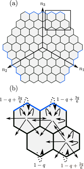
Figure 4: (Colour online). A schematic representation of the reflective hexagonal domain. Panel (a) depicts the required barriers to turn a right shift periodic domain into a fully reflective domain. Panel (b) shows the four full WS cells inside the rectangle in panel (a). In panel (b) we show how the walker tries to escape and is reflected onto the corresponding WS cell. The dotted arrows represent the modified probability of remaining on that lattice site and it depends on $q$, as indicated. Note that the probability of remaining on a corner site is $\frac{q}{6}$ greater than other boundary sites.

VI.1 Hexagonal Lattice

We consider the set of defective paired sites $B^{(r)}=\{\{\bm{b}_{1},\bm{b}^{\prime}_{1}\},\{\bm{b}_{2},\bm{b}^{\prime}_{2}\},...,\{\bm{b}_{N_{1}},\bm{b}^{\prime}_{N_{1}}\}\}$ where $N_{1}=6R+3$. Following [16], and taking $\eta_{\bm{b}_{i},\bm{b}^{\prime}_{i}}=\eta_{\bm{b}^{\prime}_{i},\bm{b}_{i}}=\frac{q}{6}$ for all $i$, the generating function of the propagator is given by

$$\widetilde{P}_{\bm{n}_{0}}^{(r)}(\bm{n},z) =\widetilde{P}_{\bm{n}_{0}}^{(p)}(\bm{n},z)-1+\frac{\det({\mathbb{K}(\bm{n},\bm{n}_{0},z)})}{\det{(\mathbb{K}(z)})},$$ (17)

where $\mathbb{K}(z)$ and $\mathbb{K}(\bm{n},\bm{n}_{0},z)$ are $(6R+3)\times(6R+3)$ matrices with elements

$$\mathbb{K}(z)_{i,k} =\frac{q}{6}\left[\widetilde{P}_{\langle\bm{b}^{\phantom{\prime}}_{k}-\bm{b}^{\prime}_{k}\rangle}^{(p)}(\bm{b}_{i},z)-\widetilde{P}_{\langle\bm{b}^{\phantom{\prime}}_{k}-\bm{b}^{\prime}_{k}\rangle}^{(p)}(\bm{b}^{\prime}_{i},z)\right]-\frac{\delta_{ik}}{z},$$ (18)

$$\mathbb{K}(\bm{n},\bm{n}_{0},z)_{i,k} =\mathbb{K}(z)_{i,k}-\frac{q}{6}\bigg{(}\widetilde{P}_{\langle\bm{b}^{\phantom{\prime}}_{k}-\bm{b}^{\prime}_{k}\rangle}^{(p)}(\bm{n},z)$$ (19)

$$\times\left[\widetilde{P}_{\bm{n}_{0}}^{(p)}(\bm{b}^{\phantom{\prime}}_{i},z)-\widetilde{P}_{\bm{n}_{0}}^{(p)}(\bm{b}^{\prime}_{i},z,)\right]\bigg{)},$$

respectively, with the notation $f_{\langle\bm{b}-\bm{b}^{\prime}\rangle}(\cdot)=f_{\bm{b}}(\cdot)-f_{\bm{b}^{\prime}}(\cdot)$.

VI.2 Honeycomb Lattice

The set of pairs of defective states is $\mathcal{B}^{(r)}=\{\{(\bm{b}^{\phantom{\prime}}_{1},m_{\bm{b}^{\phantom{\prime}}_{1}}),(\bm{b}^{\prime}_{1},m_{\bm{b}^{\prime}_{1}})\},...,\{(\bm{b}^{\phantom{\prime}}_{\mathcal{N}_{1}},m_{\bm{b}^{\phantom{\prime}}_{\mathcal{N}_{1}}}),(\bm{b}^{\prime}_{\mathcal{N}_{1}},m_{\bm{b}^{\prime}_{\mathcal{N}_{1}}})\}\}$ where the sites $(\bm{b}^{\phantom{\prime}}_{1},\bm{b}^{\phantom{\prime}}_{2}...,\bm{b}^{\phantom{\prime}}_{\mathcal{N}_{1}})$ correspond to the defective pairs required for corresponding shift in the hexagonal case making $\mathcal{N}_{1}=N_{1}$. We adjust the outgoing connections by setting $\eta_{m_{\bm{b}^{\phantom{\prime}}_{i}},m_{\bm{b}^{\prime}_{i}}}=\eta_{m_{\bm{b}^{\prime}_{i}},m_{\bm{b}_{i}}}=\frac{q}{3}$.

The generating function of the propagator is given as (see Appendix E)

$$\widetilde{\mathcal{P}}_{\bm{n}_{0},m_{0}}^{(r)}(\bm{n},m,z) =\widetilde{\mathcal{P}}_{\bm{n}_{0},m_{0}}^{(p)}(\bm{n},m,z)-1$$ (20)

$$+\frac{\det({\mathbb{L}(\bm{n},m,\bm{n}_{0},m_{0},z)})}{\det{(\mathbb{L}(z)})},$$

where $\mathbb{L}(z)$ and $\mathbb{L}(\bm{n},m,\bm{n}_{0},m_{0},z)$ are $(6R+3)\times(6R+3)$ matrices with elements

$$\mathbb{L}(z)_{i,k} =\frac{q}{3}\bigg{[}\widetilde{\mathcal{P}}_{\langle\bm{b}_{k},m_{\bm{b}_{k}}-\bm{b}^{\prime}_{k},m_{\bm{b}^{\prime}_{k}}\rangle}^{(p)}(\bm{b}_{i},m_{\bm{b}_{i}},z)-$$ (21)

$$\widetilde{\mathcal{P}}_{\langle\bm{b}_{k},m_{\bm{b}_{k}}-\bm{b}^{\prime}_{k},m_{\bm{b}^{\prime}_{k}}\rangle}^{(p)}(\bm{b}^{\prime}_{i},m_{\bm{b}^{\prime}_{i}},z)\bigg{]}-\frac{\delta_{ik}}{z},$$

and

$$\mathbb{L} (\bm{n},m,\bm{n}_{0},m_{0},z)_{i,k}=-\frac{q}{3}\widetilde{\mathcal{P}}_{\langle\bm{b}_{k},m_{\bm{b}_{k}}-\bm{b}^{\prime}_{k},m_{\bm{b}^{\prime}_{k}}\rangle}^{(p)}(\bm{n},m,z)$$ (22)

$$\times\left[\widetilde{\mathcal{P}}_{\bm{n}_{0},m_{0}}^{(p)}(\bm{b}^{\phantom{{}^{\prime}}}_{i},m_{\bm{b}^{\phantom{{}^{\prime}}}_{i}},z)-\widetilde{\mathcal{P}}_{\bm{n}_{0},m_{0}}^{(p)}(\bm{b}^{{}^{\prime}}_{i},m_{\bm{b}^{\prime}_{i}},z)\right]+\mathbb{L}(z)_{i,k},$$

respectively.

VII First-Passage Probability in Periodic Domains

Two important quantities in the dynamics of stochastic systems are the first-passage, or first hitting, probability $F_{\bm{n}_{0}}(\bm{n},t)$, and the return probability $R_{\bm{n}}(t)$. $F_{\bm{n}_{0}}(\bm{n},t)$ represents the time dependence of the probability to reach a target $\bm{n}$ from the initial condition $\bm{n}_{0}$, while $R_{\bm{n}}(t)$ represents the first time the walker returns to $\bm{n}=\bm{n}_{0}$. The generating function of these quantities are obtained via the well-known renewal equation [3], which is valid in arbitrary dimensions. The generalisation to random walks with internal states is straightforward leading to, in the $z$-domain, $\widetilde{\mathcal{F}}_{\bm{n}_{0},m_{0}}(\bm{n},m,z)=\widetilde{\mathcal{P}}_{\bm{n}_{0},m_{0}}(\bm{n},m,z)/\widetilde{\mathcal{P}}_{\bm{n},m}(\bm{n},m,z)$ and $\widetilde{\mathcal{R}}_{\bm{n},m}(z)=1-1/\widetilde{\mathcal{P}}_{\bm{n},m}(\bm{n},m,z)$ [19]. In this section, we study the differences between the first-passage temporal dependence of the left and right shift in periodically bounded domains in the presence of a single target.

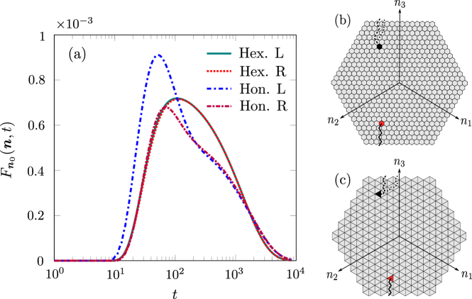
Figure 5: (Colour online). Time dependent first passage probability in periodic hexagonal and honeycomb domains. In panel (a) we present the temporal probability for both shifts in both lattices, for the initial condition and placement of the targets and initial conditions are presented in panels (b) and (c). The hexagonal lattice, panel (b), is $R=13$ (547 lattice sites) and the honeycomb lattice, panel (c), is $R=5$ (546 lattice states). In both cases, the initial condition is placed near the bottom left corner, that is $\bm{n}_{0}=(1,8,-9)$ in the hexagonal lattice, and $\bm{n}_{0},m_{0}=(1,3,-4),3$ in the honeycomb lattice, while the targets are placed across the periodic boundary near the top left corner, at $\bm{n}=(-8,0,8)$ in the hexagonal lattice and $\bm{n},m=(-4,0,4),3$ in the honeycomb lattice. This ensures that in the hexagonal shift, there is a ballistic trajectory of 10 steps for both shifts, while in the honeycomb the left shift has a ballistic trajectory of 10 steps and the right shift has a ballistic trajectory of 12 steps. We show one of these trajectories using a solid line before the walker crosses the boundary and a dashed line for the left shift and dotted line for the right shift after the walker crosses the boundary. For all curves we take $q=0.85$.

It is well known that the direct trajectories, those that travel in a more direct path from the initial condition to the target, influence the location and the mode of the first-passage probability [46]. As the chosen shift impacts the dynamics at the boundary, if the initial condition and the target are placed across the boundary from one another, the direct trajectories differ between the two shifts. This difference is greater the smaller the number of ways to reach the target (or variance in the direct trajectories), which occurs when the locations of the initial condition and the target lie only a few jumps across a boundary from one another. In this setting, by considering all the ballistic trajectories, one may expect disparities between the modes of the two shifts’ probability as even if there is an equal number of jumps to reach the target in both cases, one shift may provide more ballistic options than the other.

In Fig. 5, we show one such case by placing the walkers with identical initial conditions, near the bottom left of the domains, and placing the targets across the boundary near the top left corner (see Fig. 5 panels (b), (c)). In this setting, the lower coordination number for the honeycomb lattice ensures a lower variance in the direct trajectories. In turn, this causes the trajectories that differ between the shifts to have a greater effect on the modes of the distribution. While the difference in first-hitting dynamics is evident for the honeycomb case, to observe similar disparities for the hexagonal lattice one needs to move the initial condition and target closer to the boundary.

Despite the mode dynamics being considerably different in the honeycomb lattice, the tails of the distribution are very similar as the tail is heavily dependent on the indirect trajectories [46], i.e. the paths where the walker meanders around the domain and does not hit the target for extended periods of time. In the honeycomb case we see clearly when the indirect trajectories become dominant as it corresponds to the kinks in the temporal dependence at around $t\approx 110$.

Analytic knowledge of the propagators also allows us to readily calculate the first passage to a set of $\mathcal{M}$ targets $\{S\}=\{\bm{s}_{1},...,\bm{s}_{\mathcal{M}}\}$. This is done by considering the splitting probabilities, that is the probability of reaching one target $\bm{s}_{j}$ in $\{S\}$ before reaching any other, which is given by [15]

$$\widetilde{T}_{\bm{n}_{0}\to(\bm{s}_{j}|\{S\}-\bm{s}_{j})}(z)=\frac{\det(\mathbb{F}^{(j)}(\bm{n}_{0},z))}{\det(\mathbb{F}(z))},$$ (23)

where $\mathbb{F}(z)_{k,k}=1$, $\mathbb{F}(z)_{i,k}=\widetilde{F}_{\bm{s}_{k}}(\bm{s}_{i},z)$ and $\mathbb{F}^{(j)}(\bm{n}_{0},z)$ is the same as $\mathbb{F}(z)$ but with the $j^{\text{th}}$ column replaced with $\left[\widetilde{F}_{\bm{n}_{0}}(\bm{s}_{1},z),\widetilde{F}_{\bm{n}_{0}}(\bm{s}_{2},z),\dots,\widetilde{F}_{\bm{n}_{0}}(\bm{s}_{\mathcal{M}},z)\right]^{\intercal}$. Since the splitting probabilities represent mutually exclusive trajectories, to obtain the generating function for the first-passage to any target, one simply sums them, i.e. $\widetilde{T}_{\bm{n}_{0}\to\{S\}}=\sum_{j=1}^{\mathcal{M}}\widetilde{T}_{\bm{n}_{0}\to(\bm{s}_{j}|\{S\}-\bm{s}_{j})}(z)$. For all known internal states propagators with localised initial conditions, the analogous quantities to those in Eq. (23) are easily found, ensuring a trivial extension to the honeycomb lattice.

VIII Mean First Passage Time

Analytic knowledge of the generating functions of the first-passage and return probabilities allow us to obtain closed-form representation of their first moments ($\mathdutchcal{F}_{\bm{n}_{0}\to\bm{n}}$ and $\mathdutchcal{R}_{\bm{n}_{0}}$) in the hexagonal and honeycomb lattices found by evaluating the first derivative, with respect to $z$, of the respective probability generating function at $z=1$ [3]. The MFPT to multiple targets is also accessible via

$$\mathdutchcal{T}_{\bm{n}_{0}\to\{S\}}=\frac{\det(\mathbb{T}_{0})}{\det(\mathbb{T}_{1})-\det(\mathbb{T})},$$ (24)

a general result derived more recently in [15], where $\mathbb{T}_{ii}=0$, $\mathbb{T}_{ij}=\mathdutchcal{F}_{\bm{s}_{j}\to\bm{s}_{i}}$, $\mathbb{T}_{0_{ij}}=\mathbb{T}_{ij}-\mathdutchcal{F}_{\bm{n}_{0}\to\bm{s}_{i}}$ and $\mathbb{T}_{1_{ij}}=\mathbb{T}_{ij}-1$.

VIII.1 Hexagonal Lattice

For the hexagonal lattice, the MFPT is given by

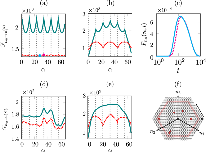
Figure 6: (Colour online). Panels (a), (b), (d) and (e) represent the MFPT in periodic (dashed lines) and reflective (solid lines) with $R=13$ hexagonal lattices. In (a) and (d), $\bm{n}_{0}=(0,0,0)$, while in (b) and (e) $\bm{n}_{0}=(13,-13,0)$. The upper two panels correspond to a single target system $\bm{s}^{(\alpha)}_{1}$, i.e. we use Eqs. (25) and (26), while for the bottom two panels, we have a system with seven targets, i.e. we use Eq. (24), retaining $\bm{s}^{(\alpha)}_{1}$ and introducing six other targets at $\bm{s}_{\{2,..7\}}=\{(-10,10,0),(0,9,-9),(0,8,-8),(7,-7,0),(0,-5,5),(-4,0,4)\}$ giving the set $\{S\}$ targets. In both cases, we move $\bm{s}^{(\alpha)}_{1}$ anti-clockwise around the $R=11$ ring of coordinates where $\bm{s}^{(1)}_{1}=(11,-11,0)$, the right most point of the ring, $\bm{s}^{(2)}_{1}=(10,-11,1)$ and so on until $\bm{s}^{(65)}_{1}=(11,-10,-1)$. Thus, in total $s^{(\alpha)}_{1}$ moved through 65 locations. We show, in panel (f), the placement of these six additional targets (dark red), the ring (light red) with the change in the placement of the target on the ring shown by the arrow and the two initial conditions (black). The vertical grey lines in panels (a), (b), (d) and (e) denote the corner points of this ring. In panel (c), we show the temporal first-passage dependence in a right shift periodic domain from $\bm{n}_{0}=(0,0,0)$ to $\bm{s}^{(28)}_{1}=(-11,11,0)$ (left dot in panel (a)) and $\bm{s}^{(34)}_{1}=(-11,5,6)$ (right dot in panel (a)), shown in, respectively, dashed and solid lines. For all plots we take $q=6/7$.

$$\mathdutchcal{F}_{\bm{n}_{0}\to\bm{n}}^{(p)_{[i]}}=\frac{2}{q}\sum_{r=0}^{R-1} \sum_{s=0}^{3r+2}\left\{\cos\left(\frac{2\pi k^{[i]}_{1}(n_{1}-n_{0_{1}})+2\pi k^{[i]}_{2}(n_{2}-n_{0_{2}})}{\Omega}\right)-1\right\}$$ (25)

$$\times\left\{\frac{1}{3}\left[\cos\left(\frac{2\pi(k_{1}^{[i]}-k_{2}^{[i]})}{\Omega}\right)+\cos\left(\frac{2\pi k_{1}^{[i]}}{\Omega}\right)+\cos\left(\frac{2\pi k_{2}^{[i]}}{\Omega}\right)\right]-1\right\}^{-1},$$

while for the MRT we confirm Kac’s lemma [47], for which, regardless of the shift, $\mathdutchcal{R}^{(p)}_{\bm{n}}=\Omega=3R^{2}+3R+1$, the inverse of the steady state probability.

Knowledge of the generating function of the reflective propagator allows us to study the same statistics in reflective domains [16]. The MFPT is given by

$$\mathdutchcal{F}^{(r)}_{\bm{n}_{0}\to\bm{n}}=\mathdutchcal{F}^{(p)}_{\bm{n}_{0}\to\bm{n}}-1+\frac{\det(\mathbb{F}-\mathbb{F}^{(1)})}{\det(\mathbb{F})},$$ (26)

where

$$\mathbb{F}_{ij}=\frac{q}{6\Omega}\left[\mathdutchcal{F}^{(p)}_{\langle\bm{b}_{j}-\bm{b}^{\prime}_{j}\rangle\to\bm{b}_{i}}-\mathdutchcal{F}^{(p)}_{\langle\bm{b}_{j}-\bm{b}^{\prime}_{j}\rangle\to\bm{b}^{\prime}_{i}}\right]+\delta_{ij},$$ (27)

and

$$\mathbb{F}^{(1)}_{ij}=\frac{q\mathdutchcal{F}^{(p)}_{\langle\bm{b}_{j}-\bm{b}^{\prime}_{j}\rangle\to\bm{n}}}{6\Omega}\left[\mathdutchcal{F}^{(p)}_{\langle\bm{n}_{0}-\bm{n}\rangle\to\bm{b}_{i}}-\mathdutchcal{F}^{(p)}_{\langle\bm{n}_{0}-\bm{n}\rangle\to\bm{b}^{\prime}_{i}}\right],$$ (28)

while the MRT is $\mathdutchcal{R}^{(r)}_{\bm{n}}=\mathdutchcal{R}^{(p)}_{\bm{n}}$, as expected.

In Fig. 6 we plot the MFPT as a function of the target location for two different initial conditions $\bm{n}_{0}=(0,0,0)$ (panels (a) and (d)) and $\bm{n}_{0}=(13,-13,0)$, the far right corner, (panels (b) and (e)). The target, $\bm{s}^{(\alpha)}_{1}$, is placed sequentially in a ring-like manner anti-clockwise around the $R=11$ circumradius of the hexagon. For the case where $\bm{n}_{0}=(0,0,0)$, although the initial displacement between the initial condition and any target is constant, rich dynamics appear the target is moved around the ring.

Owing to the symmetry of the system, in both domains, we see oscillations occurring with a wavelength of 11, the length of a side of the ring the target is moving around. Peaks are located at the corners of the $R=11$ circumradius, while the troughs correspond to the centre of the ring. At short times, it is easier for a walker to hit a target in the centre of the ring than the corner as the number of direct trajectories is greater for the centre target, seen in the modes of Fig. 6(c). Owing to the probability conserving property, the tail of $F_{\bm{n}_{0}}(\bm{n},t)$ is then slightly lower, giving a smaller MFPT. Furthermore, the MFPT in the reflective cases is roughly twice that of the corresponding periodic case. This can be understood by thinking that the periodic boundary conditions effectively double the trajectories with which the walker can reach a target compared to the reflective case.

In panel (b) there is a marked difference between the dynamics in the reflective and periodic domains. As $\bm{n}_{0}$ is the far right point of the domain, the displacement between the initial condition and a target at, for example, $\bm{s}^{(23)}_{1}=(-11,0,11)$ is much greater in the reflective domain than in the periodic domain. In the reflective case, we see a linear increase (decrease) as we move the target further away from (closer to) the initial condition. The linear increase is seen until the target moves around the first corner. We then see small oscillations where, again, targets at the centre of the ring produce a local minimum and the peaks are located at the corners. The highest peak corresponds to the target at $\bm{s}^{(34)}_{1}=(-11,11,0)$, the target furthest from the initial condition.

We now introduce six other static targets $\{\bm{s}_{2},...,\bm{s}_{6}\}$ placed at other locations within the $R=11$ ring (given explicitly in the caption of Fig. 6) and move $\bm{s}^{(\alpha)}_{1}$ sequently as before. For the $\bm{n}_{0}=(0,0,0)$ case, the introduction of more targets minimises the differences between the two boundaries compared to the one target set-up. This is likely due to the targets being placed across the whole domain meaning for many realisations, the walker will hit a target before any boundary interaction. In contrast, for $\bm{n}_{0}=(13,-13,0)$, we see similar behaviour to the one target case as in the reflective case, the initial condition renders targets on the opposite side of the domain nearly redundant as many other targets lie between them and the initial condition.

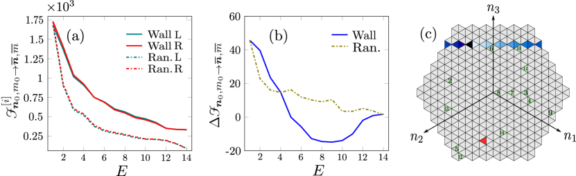
Figure 7: (Colour Online). The MFPT in the left and right shift periodic honeycomb domains as a function of the number of targets, $E$, for a randomly placed set of targets (dotted lines) and a wall of targets (solid line). Panel (a) represents the MFPT to $E$ targets, $\mathdutchcal{F}^{[i]}_{\bm{n}_{0},m_{0}\to\overline{\bm{n}},\overline{m}}$, with the bar notation denoting the option of multiple targets. Panel (b) shows the difference, $\Delta\mathdutchcal{F}_{\bm{n}_{0},m_{0}\to\overline{\bm{n}},\overline{m}}=\mathdutchcal{F}^{[\rho]}_{\bm{n}_{0},m_{0}\to\overline{\bm{n}},\overline{m}}-\mathdutchcal{F}^{[\lambda]}_{\bm{n}_{0},m_{0}\to\overline{\bm{n}},\overline{m}}$, between the two shifts. We show the order and placement of the the targets in panel (c). The first target at $\bm{n},m=(-4,0,4),3$, is shared by both set-ups and we denote its place in black. The other targets are added sequentially, which we show via the blue colour gradient from light to dark in the wall case and numerically for the random case, with targets shown in green. The initial condition at $\bm{n}_{0},m_{0}=(1,3,-4),3$ is shown in red and $q=0.85$.

For both initial conditions, we again see a maxima at $\alpha=34$, the location where $\bm{s}^{(34)}_{1}$ is located next to $\bm{s}_{2}$. As such, it renders one of these targets near redundant as if the walker is to find one of the targets, it is likely he will find both. In contrast, the shortest MFPT is when $\bm{s}^{(\alpha)}_{1}$ is dependent on the initial condition. For the case with the origin at the initial condition, the minima for both reflective and periodic is located near the centre of the bottom right side of the domain. This placement of $\bm{s}^{(\alpha)}_{1}$ fills the space and creates the most widely spread arrangement of targets meaning that a walker exploring any section of the domain is always in close proximity to a target. For $\bm{n}_{0}=(13,-13,0)$, the effect of the boundary conditions are still visible with multiple targets. In both domains, the minima naturally lie where the moving target is only a few jumps from the initial condition.

VIII.2 Honeycomb Lattice

For the honeycomb lattice, we find the MFPT as

$$\mathdutchcal{F}^{(p)_{[i]}}_{\bm{n}_{0},m_{0}\to\bm{n},m}=\bm{U}_{m}^{\intercal}\cdot\mathbb{C}\cdot\bm{U}_{m_{0}}-\bm{U}_{m}^{\intercal}\cdot\mathbb{C}\cdot\bm{U}_{m}+$$ (29)

$$\bm{U}^{\intercal}_{m}\cdot\Bigg{[}6\sum_{r=0}^{R-1}\sum_{s=0}^{3r+2}\Bigg{\{}e^{\frac{2\pi i(\bm{n}-\bm{n}_{0})\cdot\bm{k}^{[i]}}{\Omega}}\left[\bm{\mu}\left(\frac{2\pi k_{1}^{[i]}}{\Omega},\frac{2\pi k_{2}^{[i]}}{\Omega}\right)-\mathbb{I}\right]^{-1}+e^{\frac{-2\pi i(\bm{n}-\bm{n}_{0})\cdot\bm{k}^{[i]}}{\Omega}}\left[\bm{\mu}\left(\frac{-2\pi k_{1}^{[i]}}{\Omega},\frac{-2\pi k_{2}^{[i]}}{\Omega}\right)-\mathbb{I}\right]^{-1}\Bigg{\}}\Bigg{]}\cdot\bm{U}_{m_{0}}$$

$$-\bm{U}^{\intercal}_{m}\cdot\bigg{[}6\sum_{r=0}^{R-1}\sum_{s=0}^{3r+2}\Bigg{\{}\left[\bm{\mu}\left(\frac{2\pi k_{1}^{[i]}}{\Omega},\frac{2\pi k_{2}^{[i]}}{\Omega}\right)-\mathbb{I}\right]^{-1}+\left[\bm{\mu}\left(\frac{-2\pi k_{1}^{[i]}}{\Omega},\frac{-2\pi k_{2}^{[i]}}{\Omega}\right)-\mathbb{I}\right]^{-1}\Bigg{\}}\Bigg{]}\cdot\bm{U}_{m}$$

where $\mathbb{C}$ is a $6\times 6$ symmetric circulant matrix with the first row $c=\left[5-\frac{9}{q},5-\frac{4}{q},5-\frac{3}{q},5-\frac{4}{q},5-\frac{3}{q},5-\frac{4}{q}\right]$ such that $\mathbb{C}_{ij}=c_{j-i\ (\mathrm{mod}\ 6)}$. The term $\bm{U}_{m}^{\intercal}\cdot\mathbb{C}\cdot\bm{U}_{m_{0}}-\bm{U}_{m}^{\intercal}\cdot\mathbb{C}\cdot\bm{U}_{m}$ is independent of the choice of shift and governs the MFPT in the degenerate $R=0$ case, which is periodic in $|m-m_{0}|$ and given explicitly in Eq. (56). It gives the MFPT for any $m,m_{0}$ pairs that are either one jump away or those that are two jumps away from one another (see Fig. 1b when R=0 for visual understanding). We again confirm Kac’s lemma as the MRT is found to be $\mathdutchcal{R}^{(p)}_{\bm{n}_{0},m_{0}}=6\Omega$, the number of states in the lattice. For the reflective case, one obtains similar expressions to the hexagonal lattice with reflecting boundaries (see Appendix F.2).

Using Eq. (29) we study the differences between the MFPT of the two shifts as a function of the number of targets. We sequentially introduce targets in two ways, either building a ‘wall’ of targets along the top of the domain or placing targets at random locations, with both set-ups shown pictorially in panel (c) of Fig. 7. In both the random and the ‘wall’ placement of targets, the initial condition and the location of the first target correspond to the set-up used to obtain the full FP probability given in Fig. 5.

As Fig. 7, Panel (a) shows, for both target set-ups, adding targets lowers the MFPT, as expected. In the randomly placed target case, an increase in the number $E$ of targets reduces the differences between the MFPTs, if the added target is placed in the bulk of the domain, seen in Fig. 7, Panel (b). This reduction is due to the increasing likelihood that the walker reaches the target before any boundary interactions occur. If, on the other hand, the new target is placed on, or very closed to, the boundary ($E=5$, $E=9$ and $E=12$) slight increases are seen in $\Delta\mathdutchcal{F}_{\bm{n}_{0},m_{0}\to\bm{n},m}$ further emphasising the importance of boundary interactions in the periodic propagators.

In the case of the ‘wall’, we add the targets to the right of the initial target until we reach it again from the left. In this case we see a dramatic convergence between the two shifts before the mean of the right shift becomes lower. With a wall of targets placed near the top of the domain, the easiest route for the walker to complete its search is the few steps across the boundary. As exemplified by the higher first-passage probability mode of the left shift honeycomb walker (Fig. 5), when there are few targets, the searcher benefits from the left shift boundary condition since the distance to the target is smaller. However, as we build the wall to the right, this advantage lessens until sufficient targets are added such that it is more beneficial to utilise the right shift walker. Finally, when the wall is complete ($E=14$) we see negligible differences between the two shifts.

IX Conclusions

The implementation of the method of images to obtain periodically bounded LRW in square geometries has been known for some time [4, 37]. Somewhat surprisingly, the same could not be said about hexagonal lattices. Here, we have constructed the image set for a lattice in HCC and derived the exact spatio-temporal dynamics for a LRW on a periodic hexagonal and honeycomb lattice. By generalising the defect technique to hexagonal geometries we have found the absorbing and reflecting propagators for both lattices. We have then utilised these propagators to obtain expressions such as the return and first-passage probabilities and their means.

We note that while we limit ourselves to deploying the defect technique for the dynamics in hexagonally constrained spatial domains, it is possible to place both absorbing or reflecting sites in such a way as to confine the domain to other shapes, for example, a triangle. Moreover, the formalism may be applied to other periodic propagators in hexagonal geometries, for example, a biased LRW [11], a resetting random walker [13] or when the space is composed of different media [14]. Dynamics on other lattice geometries are also available through our internal states procedure. For example, by placing three internal states in a triangular structure, one can create the so-called tri-hexagonal lattice [48] or with four internal states, one can achieve a square-octagon tessellation seen in the theorised T-graphene structure [49]. Other potential directions include finding continuum limits of the periodic propagator and placing both absorbing defects [38] or reflecting defects [50] to obtain diffusive dynamics in hexagonally shaped domains, avoiding the need to solve the diffusion equation numerically in these geometries. We conclude by noting other potential applications of our work. These include modelling neutron diffusion in a nuclear reactor core [51, 52], the transmission of an infectious pathogen in a population of territorial animals [22, 7, 53, 23], diffusion on a SWCN with topological defects such as dislocations [54], and amoeboid migration in Petri dishes with hexagonally placed micropillars [55].

Appendix A Placement of Images

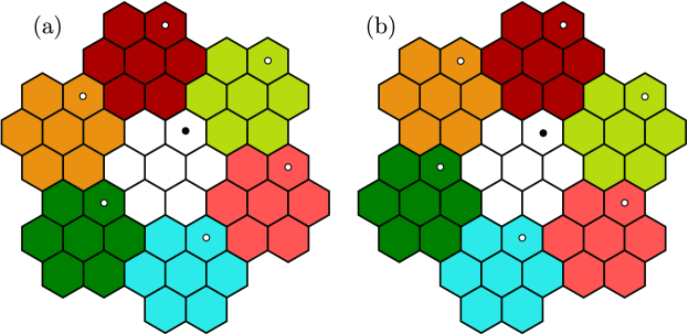
Figure 8: (Colour online). A schematic representation of the nearest-neighbour images for panel (a), the left shift, and panel (b), the right shift, in an $R=1$ domain. In this case, we show in the central domain, the LRW starting location as a filled circle while the first ring of images has open circles. For ease of visual comparison between the left and right shift, each hexagon in the nearest-neighbour image ring is coloured differently.

Figure 8 shows the first ring of the infinite images for an $R=1$ domain as per discussion in Sec. IV. We refer to the shift with respect to the location of the top red image, that is whether it is to the left or the right of the main domain.

Appendix B Derivation of the Periodic Hexagonal Propagator

Using the periodic image set, Eqs. (10) and (11), in the unbounded Green’s lattice function, Eq. (4) in the main text, and isolating the image contribution in the exponential, we obtain

$$\widetilde{P}^{[i]}_{\bm{n}_{0}}(n_{1},n_{2},z)=\frac{1}{(2\pi)^{2}}\int_{-\pi}^{\pi}\int_{-\pi}^{\pi}\sum_{m_{1}=-\infty}^{\infty}\sum_{m_{2}=-\infty}^{\infty}\frac{e^{i[(\bm{n}-\bm{n}_{0})\cdot\bm{k}]}e^{i[\bm{m}\cdot\mathbb{D}_{[i]}\cdot\bm{k}]}}{1-z\mu(k_{1},k_{2})}dk_{1}k_{2},$$ (30)

where $\bm{m}=(m_{1},m_{2})$, and for the right shift

$$\mathbb{D}_{[\rho]}=\begin{bmatrix}-R&-R-1\\ 2R+1&-R\end{bmatrix},$$ (31)

while for the left shift

$$\mathbb{D}_{[\lambda]}=\begin{bmatrix}2R+1&-R-1\\ -R&2R+1\end{bmatrix}.$$ (32)

Equations (30), (31), and (32) allow us to connect with literature on Fourier analysis in hexagonal domains [56, 39] and utilise the distributional form of the Poisson summation formula associated with the hexagonal lattice

$$\sum_{m_{1}=-\infty}^{\infty}\sum_{m_{2}=-\infty}^{\infty}e^{i[\bm{m}\cdot\mathbb{D}_{[i]}\cdot\bm{k}]}=\frac{(2\pi)^{2}}{\Omega}\sum_{m_{1}=-\infty}^{\infty}\sum_{m_{2}=-\infty}^{\infty}\delta(\bm{k}-2\pi\mathbb{D}_{[i]}^{-1}\cdot\bm{m}^{\intercal}),$$ (33)

where $\Omega=3R^{2}+3R+1$, the number of sites in the hexagonal lattice. The equivalent result for the square lattice can be found in [57]. We note here the importance of dropping the $n_{3}$ dependence from Eq. (2). If the full three co-ordinate representation of HCC was chosen, $\mathbb{D}_{[\rho,\lambda]}$ would be a $3\times 3$ matrix, with three linearly dependent rows making $\mathbb{D}_{[i]}$ singular matrices.

Applying Eq. (33) on Eq. (30) and shifting the integral limits, due to the periodicity of the integrand, we obtain

$$\widetilde{P}^{[i]}_{\bm{n}_{0}}(n_{1},n_{2},z)=\int_{-\varepsilon}^{2\pi-\varepsilon}\int_{-\varepsilon}^{2\pi-\varepsilon}\sum_{m_{1}=-\infty}^{\infty}\sum_{m_{2}=-\infty}^{\infty}\frac{e^{i[(\bm{n}-\bm{n}_{0})\cdot\bm{k}]}\delta(\bm{k}-2\pi\mathbb{D}_{[i]}^{-1}\cdot\bm{m}^{\intercal})}{\Omega\left[1-z\mu(k_{1},k_{2})\right]}dk_{1}dk_{2},$$ (34)

where the parameter $0<\varepsilon\leq\frac{2\pi}{\Omega}$, avoids having a singularity of the Dirac delta on the integral bound. The values where the Dirac delta is non-zero are given by

$$k^{[\rho]}_{1} =\frac{2\pi}{\Omega}[-Rm_{1}+(R+1)m_{2}],$$ (35)

$$k^{[\rho]}_{2} =\frac{-2\pi}{\Omega}[(2R+1)m_{1}+Rm_{2}],$$

for the right shift and

$$k^{[\lambda]}_{1} =\frac{2\pi}{\Omega}[(2R+1)m_{1}+(R+1)m_{2}],$$ (36)

$$k^{[\lambda]}_{2} =\frac{2\pi}{\Omega}[Rm_{1}+(2R+1)m_{2}],$$

for the left shift.

To proceed, one finds the values of $m_{1}$ and $m_{2}$, which lead to singularities that lie within the integral bounds where each $(m_{1},m_{2})$ corresponds to a unique point in the finite domain. However, due to the non-orthogonality of the coordinate points, one cannot independently sum $m_{1}$ and $m_{2}$ along the length of each axis, as one does for the square lattice. To overcome this, we parameterise $k^{[i]}_{1},k^{[i]}_{2}$ via Eq. (13), alongside their corresponding negative value, and create the nested summation in Eq. (12) in the main text. Figure 9 shows the validity of this parameterisation for the left (panel (a)) and right (panel (b)) shift. Upon substituting these parameterised values into Eq. (34) and simplifying the complex exponential, one obtains the exact periodic propagator Eq. (12).

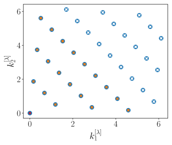
(a)

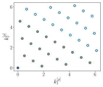
(b)

Figure 9: The $k_{1}^{[i]}$, $k_{2}^{[i]}$ value that give a singularity of the Dirac delta in Eq. (34) for an $R=3$ domain for (a) the left shift and (b) the right shift. The large circles represent $k_{1}^{[i]}$, $k_{2}^{[i]}$ found numerically by summing over $m_{1}$, $m_{2}$. The corresponding parameterised values, Eq. (13) are represented by crosses. The first three ($R$) diagonal rows correspond to the positive $k_{1}^{[i]}$, $k_{2}^{[i]}$ values, while the remaining three are the negative ones, where for ease of visualisation, we have added a $2\pi$ phase to the negative terms. The term corresponding to the steady state is shown at $(0,0)$. Note that in this case, there are $\Omega=37$ points that need to be paramaterised.

Appendix C Derivation of the Periodic Honeycomb Propagator

Starting from Eq. (7) in the main text and applying the images defined in Sec. IV leads to

$$\widetilde{\bm{\mathcal{P}}}^{(p)_{[i]}}_{\bm{n}_{0},m_{0}}(n_{1},n_{2},z)=\frac{1}{\Omega}\int_{-\pi}^{\pi}\int_{-\pi}^{\pi}\sum_{m_{1}=-\infty}^{\infty}\sum_{m_{2}=-\infty}^{\infty}\delta(\bm{k}-2\pi\mathbb{D}_{[i]}^{-1}\cdot\bm{m}^{\intercal})e^{i[(\bm{n}-\bm{n}_{0})\cdot\bm{k}]}\left[\mathbb{I}-z\bm{\mu}(k_{1},k_{2})\right]^{-1}\cdot\bm{U}_{m_{0}}dk_{1}dk_{2}.$$ (37)

Expanding $\left[\mathbb{I}-z\bm{\mu}(k_{1},k_{2})\right]^{-1}$ in powers of $z$, $\left[\mathbb{I}-z\bm{\mu}(k_{1},k_{2})\right]^{-1}=\sum_{t=0}^{\infty}\left[z\bm{\mu}(k_{1},k_{2})\right]^{t}$ and shifting the integral limits one has

$$\bm{\mathcal{P}}^{(p)_{[i]}}_{\bm{n}_{0},m_{0}}(n_{1},n_{2},t)=\frac{1}{\Omega}\int_{-\varepsilon}^{2\pi-\varepsilon}\int_{-\varepsilon}^{2\pi-\varepsilon}\sum_{m_{1}=-\infty}^{\infty}\sum_{m_{2}=-\infty}^{\infty}\delta(\bm{k}-2\pi\mathbb{D}_{[i]}^{-1}\cdot\bm{m}^{\intercal})e^{i[(\bm{n}-\bm{n}_{0})\cdot\bm{k}]}\bm{\mu}(k_{1},k_{2})^{t}\cdot\bm{U}_{m_{0}}dk_{1}dk_{2}.$$ (38)

Using the known parametrisation of the Dirac delta (see Appendix B), one finds the closed-form solution for the honeycomb lattice, shown in Eq. (14) of the main text.

C.1 Steady state behaviour in the honeycomb lattice

Since the eigenvalues and eigenvectors of $\bm{\mu}\left(0,0\right)$ are readily available, one can diagonalise the symmetric matrix $\bm{\mu}\left(0,0\right)=\mathbb{P}\mathbb{E}\mathbb{P}^{-1}$ where $\mathbb{E}_{1,1}=1$, $\mathbb{E}_{i,i}=1-q$, $2\leq i\leq 5$, $\mathbb{E}_{6,6}=1-2q$, $\mathbb{E}_{i,j}=0$ otherwise, and

$$\mathbb{P}=\frac{1}{\sqrt{6}}\begin{bmatrix}-1&1&0&-\sqrt{3}&0&-1\\ 1&1&-\sqrt{3}&0&-1&0\\ -1&1&0&0&0&2\\ 1&1&0&0&2&0\\ -1&1&0&\sqrt{3}&0&-1\\ 1&1&\sqrt{3}&0&-1&0\\ \end{bmatrix}.$$ (39)

For $0<q<1$, $\mathbb{P}\mathbb{E}^{t}\mathbb{P}^{-1}\to\mathbb{P}\overline{\mathbb{E}}\mathbb{P}^{-1}$ as $t\to\infty$, where $\overline{\mathbb{E}}_{1,1}=1$ and $\overline{\mathbb{E}}_{i,j}=0$ otherwise. Evaluating $\mathbb{P}\overline{\mathbb{E}}\mathbb{P}^{-1}$, it is straightfoward to find $\bm{\mu}(0,0)^{t}=\frac{1}{6}\mathbb{J}$ as $t\to\infty$.

For the $q=1$ case one has to be more careful as $\lim_{t\to\infty}\mathbb{E}_{6,6}=\lim_{t\to\infty}(-1)^{t}$. Here, $\bm{\mu}(0,0)$ is a hollow Toeplitz matrix with alternating bands of 0 and $\frac{1}{3}$. By inspecting this matrix, it is clear that all odd powers of $t$ revert $\bm{\mu}(0,0)$ onto itself, while even powers of $t$ ‘swap’ the bands, giving rise to the alternating steady state probabilities in this case.

Appendix D Propagator with Absorbing Defects with Internal States

Here we outline the generalisation of the defect technique on the lattice to random walks with internal states. It follows closely to, and generalises, the derivation in Sec. 2.1 of [15].

We begin with the general Master equation governing the dynamics of the occupation probability of a random walker in a lattice with defective internal states $(\bm{b},m_{\bm{b}})$ in the set $\mathcal{B}$ with $\mathcal{N}$ defects

$$\mathcal{P}(\bm{n},m,t+1) =\sum_{\bm{n^{\prime}}}\sum_{m^{\prime}}A(\bm{n},m,\bm{n^{\prime}},m^{\prime})\mathcal{P}(\bm{n^{\prime}},m^{\prime},t),\;\;\;\bm{n},m\notin\mathcal{B}$$ (40)

$$\mathcal{P}(\bm{b}_{i},m_{\bm{b}_{i}},t+1) =(1-\rho_{\bm{b}_{i},m_{\bm{b}_{i}}})\sum_{\bm{n^{\prime}}}\sum_{m^{\prime}}A(\bm{b}_{i},m_{\bm{b}_{i}},\bm{n^{\prime}},m^{\prime})\mathcal{P}(\bm{n^{\prime}},m^{\prime},t),\;\;\;\bm{b}_{i},m_{\bm{b}_{i}}\in\mathcal{B},$$

i.e. $i\in\{1,...,|\mathcal{B}|\}$, $A(\bm{n},m,\bm{n^{\prime}},m^{\prime})$ is the transition probability tensor from state $\bm{n},m$ to state $\bm{n}^{\prime},m^{\prime}$, and where $\rho_{\bm{b}_{i},m_{\bm{b}_{i}}}$ $(0\leq\rho_{\bm{b}_{i},m_{\bm{b}_{i}}}\leq 1)$ governs the probability of getting absorbed at defect $\bm{b}_{i},m_{\bm{b}_{i}}$ where $\rho_{\bm{b}_{i},m_{\bm{b}_{i}}}=1$ represents perfect trapping efficiency at that site. To proceed, one first considers $\rho_{\bm{b}_{i},m_{\bm{b}_{i}}}\neq 1$ case.

For convenience, we combine Eq. (40) into one equation

$$\mathcal{P}(\bm{n},m,t+1)=\sum_{\bm{n^{\prime}}}\sum_{m^{\prime}}\bigg{[}A(\bm{n},m,\bm{n^{\prime}},m^{\prime})\mathcal{P}(\bm{n^{\prime}},m^{\prime},t)-\sideset{}{{}^{\prime}}{\sum}_{\bm{b}}\sum_{m_{\bm{b}}}\rho_{\bm{b},m_{\bm{b}}}\delta_{\bm{n}\bm{b}}\delta_{mm_{\bm{b}}}A(\bm{b},m_{\bm{b}},\bm{n^{\prime}},m^{\prime})\mathcal{P}(\bm{n}^{\prime},m^{\prime},t)\bigg{]},$$ (41)

where the primed summation is over all defective sites containing a defective state, and the following summation is over all the states $m_{\bm{b}}$ in that site. The formal solution is simply the propagator of the defect free problem plus the propagator convoluted in time and space with the known, defect-free term [15]. Calling $\Psi_{\bm{n}_{0},m_{0}}(\bm{n},m,t)$ the defect-free propagator (the periodic propagator in this case) and applying the localised initial condition $\mathcal{P}(\bm{n},m,0)=\delta_{\bm{n}\bm{n}_{0}}\delta_{mm_{0}}\left[(1-\rho_{\bm{n}_{0}m_{0}})\delta_{\bm{n}_{0}m_{0}\in\mathcal{B}}+\delta_{\bm{n}_{0}m_{0}\notin\mathcal{B}}\right]$ one obtains, in $z$-domain,

$$\widetilde{\mathcal{P}}_{\bm{n}_{0},m_{0}}(\bm{n},m,z)=\widetilde{\Psi}_{\bm{n}_{0},m_{0}}(\bm{n},m,z)-\sideset{}{{}^{\prime}}{\sum}_{\bm{b}}\sum_{m_{\bm{b}}}\frac{\rho_{\bm{b},m_{\bm{b}}}}{1-\rho_{\bm{b},m_{\bm{b}}}}\widetilde{\Psi}_{\bm{b},m_{\bm{b}}}(\bm{n},m,z)\widetilde{\mathcal{P}}_{\bm{n}_{0},m_{0}}(\bm{b},m_{\bm{b}},z).$$ (42)

After setting $\bm{n},m$ to all absorbing sites $\bm{b},m_{\bm{b}}$, Eq. (42) can be solved via Cramer’s rule giving

$$\widetilde{\mathcal{P}}_{\bm{n}_{0},m_{0}}(\bm{b}_{j},m_{\bm{b}_{j}},z)=(1-\rho_{\bm{b}_{j},m_{\bm{b}_{j}}})\frac{\det(\mathbb{H}^{(j)}(\bm{\rho},\bm{n}_{0},m_{0},z))}{\det(\mathbb{H}(\bm{\rho},z))}.$$ (43)

Equation (43) represents the generating function of the probability of being at defective site $\bm{b}_{j}$, $m_{\bm{b}_{j}}$ at time $t$ and not having been absorbed in any of the other sites in the set $\mathcal{B}$.

The elements in the matrix $\mathbb{H}(\bm{\rho},z)$ are given as $\mathbb{H}_{k,k}(\bm{\rho},z)=1+\rho_{\bm{b}_{k},m_{\bm{b}_{k}}}+\rho_{\bm{b}_{k},m_{\bm{b}_{k}}}\widetilde{\Psi}_{\bm{b}_{k},m_{\bm{b}_{k}}}(\bm{b}_{k},m_{\bm{b}_{k}},z)$ and $\mathbb{H}_{i,k}(\bm{\rho},z)=\rho_{\bm{b}_{k},m_{\bm{b}_{k}}}\widetilde{\Psi}_{\bm{b}_{k},m_{\bm{b}_{k}}}(\bm{b}_{i},m_{\bm{b}_{i}},z)$ and $\mathbb{H}^{(j)}(\bm{\rho},\bm{n}_{0},m_{0},z)$ is the same as $\mathbb{H}(\rho,z)$ but with the $j^{\text{th}}$ column replaced with $\left(\widetilde{\Psi}_{\bm{n}_{0},m_{0}}(\bm{b}_{1},m_{\bm{b}_{1}},z),...,\widetilde{\Psi}_{\bm{n}_{0},m_{0}}(\bm{b}_{\mathcal{N}},m_{\bm{b}_{\mathcal{N}}},z)\right)^{\intercal}$.

Substituting Eq. (43) into Eq. (42) and taking the limit $\rho_{\bm{b}_{i},m_{\bm{b}_{i}}}\to 1$ gives us the defective propagator given in Eq. (16) of the main text, where we have taken $\rho_{\bm{b}_{k},m_{\bm{b}_{k}}}=1$, for all $k$, to model the fully absorbing boundary. As such, in Eq. (16), we have dropped the $\rho$ dependence in $\mathbb{H}$.

Appendix E Propagator with Inert Spatial Heterogeneities with Internal States

Here we outline the derivation of the defect technique to account for inert spatial heterogeneities in random walks with internal states. It follows closely to and generalises [16] (see Section I of the Supplementary Material). In this case, the defects appear in pairs $\mathcal{B}=\{\{(\bm{b}_{1},m_{\bm{b}_{1}}),(\bm{b}^{\prime}_{1},m_{\bm{b}^{\prime}_{1}})\},...,\{(\bm{b}_{\mathcal{N}},m_{\bm{b}_{\mathcal{N}}}),(\bm{b}^{\prime}_{\mathcal{N}},m_{\bm{b}^{\prime}_{\mathcal{N}}})\}\}$, that is, in the case of the reflective propagator, the boundary states and their respective neighbour across the periodic boundary.

The dynamics are given by

$$\mathcal{P}(\bm{n},m,t+1)=\sum_{\bm{n^{\prime}}}\sum_{m^{\prime}}A(\bm{n},m,\bm{n^{\prime}},m^{\prime})\mathcal{P}(\bm{n^{\prime}},m^{\prime},t),$$ (44)

when the walker is not on a defective site. Instead, when the walker is on any defective site we have

$$\mathcal{P}(\bm{b}_{i},m_{\bm{b}_{i}},t+1)=\sum_{\bm{n^{\prime}}}\sum_{m^{\prime}}A(\bm{b}_{i},m_{\bm{b}_{i}},\bm{n^{\prime}},m^{\prime})\mathcal{P}(\bm{n^{\prime}},m^{\prime},t)+\eta_{m_{\bm{b}^{\prime}_{i}},m_{\bm{b}_{i}}}\mathcal{P}(\bm{b}_{i},m_{\bm{b}_{i}},t)-\eta_{m_{\bm{b}_{i}},m_{\bm{b}^{\prime}_{i}}}\mathcal{P}(\bm{b}^{\prime}_{i},m_{\bm{b}^{\prime}_{i}},t),$$ (45)

$$\mathcal{P}(\bm{b}^{\prime}_{i},m_{\bm{b}^{\prime}_{i}},t+1)=\sum_{\bm{n^{\prime}}}\sum_{m^{\prime}}A(\bm{b}_{i},m_{\bm{b}_{i}},\bm{n^{\prime}},m^{\prime})\mathcal{P}(\bm{n^{\prime}},m^{\prime},t)+\eta_{m_{\bm{b}_{i}},m_{\bm{b}^{\prime}_{i}}}\mathcal{P}(\bm{b}^{\prime}_{i},m_{\bm{b}^{\prime}_{i}},t)-\eta_{m_{\bm{b}^{\prime}_{i}},m_{\bm{b}_{i}}}\mathcal{P}(\bm{b}_{i},m_{\bm{b}_{i}},t).$$ (46)

Once again, combining Eqs. (45) and (46) into one equation and taking the $z$-transform, one obtains

$$\widetilde{\mathcal{P}}(\bm{n},m,z)-\mathcal{P}(\bm{n},m,0)=\sum_{\bm{n^{\prime}}}\sum_{m^{\prime}}A(\bm{n},m,\bm{n^{\prime}},m^{\prime}) \widetilde{\mathcal{P}}(\bm{n^{\prime}},m^{\prime},z)+z\sum_{i=1}^{\mathcal{N}}\Big{\{}\delta_{\bm{b}_{i}\bm{n}}\delta_{m_{\bm{b}_{i}}m}-\delta_{\bm{b}^{\prime}_{i}\bm{n}}\delta_{m_{\bm{b}^{\prime}_{i}}m}\Big{\}}$$ (47)

$$\times\left[\eta_{m_{\bm{b}_{i}},m_{\bm{b}^{\prime}_{i}}}\widetilde{\mathcal{P}}(\bm{b}^{\prime}_{i},m_{\bm{b}^{\prime}_{i}},z)-\eta_{m_{\bm{b}^{\prime}_{i}},m_{\bm{b}_{i}}}\widetilde{\mathcal{P}}(\bm{b}_{i},m_{\bm{b}_{i}},z)\right],$$

with the parameters $\eta_{\bm{u},\bm{v}}$ defined in the main text. Assuming the defect-free solution $\widetilde{\Psi}_{\bm{n}_{0},m_{0}}(\bm{n},m,z)$ is known, i.e. the propagator of Eq. (44), which in our case we again take as the periodic propagator, the general solution of Eq. (47) for a localised initial condition $\mathcal{P}(\bm{n},m,0)=\delta_{\bm{n}\bm{n}_{0}}\delta_{mm_{0}}$ is

$$\widetilde{\mathcal{P}}_{\bm{n}_{0},m_{0}}(\bm{n},m,z) =\widetilde{\Psi}_{\bm{n}_{0},m_{0}}(\bm{n},m,z)+z\sum_{j=1}^{\mathcal{N}}\widetilde{\Psi}_{\langle\bm{b}_{j},m_{\bm{b}_{j}}-\bm{b}^{\prime}_{j},m_{\bm{b}^{\prime}_{j}}\rangle}(\bm{n},m,z)$$ (48)

$$\times\left[\eta_{m_{\bm{b}_{j}},m_{\bm{b}^{\prime}_{j}}}\widetilde{\mathcal{P}}(\bm{b}^{\prime}_{j},m_{\bm{b}^{\prime}_{j}},z)-\eta_{m_{\bm{b}^{\prime}_{j}},m_{\bm{b}_{j}}}\widetilde{\mathcal{P}}(\bm{b}_{i},m_{\bm{b}_{i}},z)\right].$$

We again solve by creating $\mathcal{N}$ simultaneous equations (for each defect pair). Using Cramer’s rule we obtain the propagator,

$$\widetilde{\mathcal{P}}_{\bm{n}_{0},m_{0}}(\bm{n},m,z)=\widetilde{\Psi}_{\bm{n}_{0},m_{0}}(\bm{n},m,z)-\sum_{j=1}^{\mathcal{N}}\widetilde{\Psi}_{\langle\bm{b}_{j},m_{\bm{b}_{j}}-\bm{b}^{\prime}_{j},m_{\bm{b}^{\prime}_{j}}\rangle}(\bm{n},m,z)\frac{\det(\mathbb{S}(\bm{n}_{0},m_{0},z))}{\det(\mathbb{S}(z))},$$ (49)

where

$$\mathbb{S}(z)_{i,k}=\eta_{\bm{b}^{\prime}_{i},\bm{b}_{i}}\widetilde{\Psi}_{\langle\bm{b}_{k},m_{\bm{b}_{k}}-\bm{b}^{\prime}_{k},m_{\bm{b}^{\prime}_{k}}\rangle}(\bm{b}_{i},m_{\bm{b}_{i}},z)-\eta_{\bm{b}_{i},\bm{b}^{\prime}_{i}}\widetilde{\Psi}_{\langle\bm{b}_{k},m_{\bm{b}_{k}}-\bm{b}^{\prime}_{k},m_{\bm{b}^{\prime}_{k}}\rangle}(\bm{b}^{\prime}_{i},m_{\bm{b}^{\prime}_{i}},z)-\frac{\delta_{ik}}{z},$$ (50)

and $\mathbb{S}(\bm{n}_{0},m_{0},z)$ the same as $\mathbb{S}(z)$ but with the $j^{\text{th}}$ column replaced with

$$\Big{[}(\eta_{m_{\bm{b}^{\prime}_{1}},m_{\bm{b}_{1}}}\widetilde{\Psi}_{\bm{n}_{0},m_{0}}(\bm{b}_{1},m_{\bm{b}^{\prime}_{1}},z)-\eta_{m_{\bm{b}_{1}},m_{\bm{b}^{\prime}_{1}}}\widetilde{\Psi}_{\bm{n}_{0},m_{0}}(\bm{b}^{\prime}_{1},m_{\bm{b}^{\prime}_{1}},z),...,$$ (51)

$$\eta_{m_{\bm{b}^{\prime}_{\mathcal{N}}},m_{\bm{b}_{\mathcal{N}}}}\widetilde{\Psi}_{\bm{n}_{0},m_{0}}(\bm{b}_{\mathcal{N}},m_{\bm{b}_{\mathcal{N}}},z)-\eta_{m_{\bm{b}_{\mathcal{N}}},m_{\bm{b}^{\prime}_{\mathcal{N}}}}\widetilde{\Psi}_{\bm{n}_{0},m_{0}}(\bm{b}^{\prime}_{\mathcal{N}},m_{\bm{b}^{\prime}_{\mathcal{N}}},z)\Big{]}^{{}^{\intercal}}.$$

Evaluating the sum in Eq. (49) explicitly and taking $\eta_{m_{\bm{b}_{i}},m_{\bm{b}^{\prime}_{i}}}=\eta_{m_{\bm{b}^{\prime}_{i}},m_{\bm{b}_{i}}}=\frac{q}{3}$, i.e. the outgoing probability from each site in the defect-free honeycomb lattice, one finds the honeycomb reflective propagator as shown in Eq. (20) in the main text.

Appendix F Honeycomb MFPT and MRT

F.1 Periodic Boundary Conditions

Using the $z$-transform Eq. (14), one finds the return probability as

$$\mathcal{R}^{(p)_{[i]}}_{\bm{n}_{0},m_{0}}(z)=1-$$ (52)

$$\frac{\Omega}{\bm{U}^{\intercal}_{m_{0}}\cdot\left[[\mathbb{I}-z\bm{\mu}(0,0)]^{-1}+\sum_{r=0}^{R-1}\sum_{s=0}^{3r+2}\Bigg{\{}\left[\mathbb{I}-z\bm{\mu}\left(\frac{2\pi k_{1}^{[i]}}{\Omega},\frac{2\pi k_{2}^{[i]}}{\Omega}\right)\right]^{-1}+\left[\mathbb{I}-z\bm{\mu}\left(\frac{-2\pi k_{1}^{[i]}}{\Omega},\frac{-2\pi k_{2}^{[i]}}{\Omega}\right)\right]^{-1}\Bigg{\}}\right]\cdot\bm{U}_{m_{0}}}.$$

Owing to the recurrence of the random walk, the matrix $[\mathbb{I}-z\bm{\mu}(0,0)]$ is singular at $z=1$. Denoting the summand in Eq. (52) as $\mathbb{M}^{[i]}(r,s)$ and multiplying the top and bottom of the fraction by $\det([\mathbb{I}-z\bm{\mu}(0,0)])$, we find

$$\mathcal{R}^{(p)_{[i]}}_{\bm{n}_{0},m_{0}}(z)=1-\frac{\Omega\det([\mathbb{I}-z\bm{\mu}(0,0)])}{\bm{U}^{\intercal}_{m_{0}}\cdot\left[\text{Inv}\left([\mathbb{I}-z\bm{\mu}(0,0)]\right)+\det([\mathbb{I}-z\bm{\mu}(0,0)])\sum_{r=0}^{R-1}\sum_{s=0}^{3r+2}\mathbb{M}^{[i]}(r,s)\right]\cdot\bm{U}_{m_{0}}},$$ (53)

where the notation $\text{Inv}(\cdot)$ denotes the inverse matrix multiplied by its determinant. Evaluating $\frac{\partial\mathcal{R}^{[i]}_{\bm{n}_{0},m_{0}}}{\partial z}\Bigr{|}_{z=1}$, and utilising the property $\det([\mathbb{I}-z\bm{\mu}(0,0)])\Bigr{|}_{z=1}=0$, we obtain for either shift,

$$\mathdutchcal{R}^{(p)}_{\bm{n}_{0},m_{0}}=-\frac{\Omega\left(\frac{\partial\det([\mathbb{I}-z\bm{\mu}(0,0)])}{\partial z}\Bigr{|}_{z=1}\right)}{\bm{U}^{\intercal}_{m_{0}}\cdot\text{Inv}(\mathbb{I}-\bm{\mu}(0,0))\cdot\bm{U}_{m_{0}}}.$$ (54)

Upon inspection of the $6\times 6$ matrix, one finds $\frac{\partial\det([\mathbb{I}-z\bm{\mu}(0,0)])}{\partial z}\Bigr{|}_{z=1}=-2q^{5}$ and $\text{Inv}(\mathbb{I}-\bm{\mu}(0,0))=\frac{q^{5}}{3}\mathbb{J}$, where $\mathbb{J}$ again denotes an all ones matrix. Using these values in Eq. (54), we confirm Kac’s lemma obtaining $\mathdutchcal{R}_{\bm{n}_{0},m_{0}}=6\Omega$, the number of states in the domain.

Following the same procedure on the honeycomb first passage probability, one obtains Eq. (29) of the main text. When $R=0$, the periodic honeycomb MFPT, Eq. (29), reduces to

$$\mathdutchcal{F}^{(p)}_{m_{0}\to m}=\sum_{i=1}^{6}\lambda_{i}\left(\bm{U}_{m}^{\intercal}\cdot\bm{u}_{i}\cdot\bm{u}_{i}^{\intercal}\cdot\bm{U}_{m_{0}}-\bm{U}_{m}^{\intercal}\cdot\bm{u}_{i}\cdot\bm{u}_{i}^{\intercal}\cdot\bm{U}_{m}\right),$$ (55)

where $\bm{u}_{i}$ are an orthonormal basis formed of the right eigenvectors associated with the eigenvalues of $\mathbb{C}$, $\lambda_{k}=\sum_{l=0}^{5}c_{l}e^{\frac{2\pi i(k-1)l}{6}}$, $k\in\{1,6\}$. Evaluating Eq. (55), one finds

$$\mathdutchcal{F}^{(p)}_{m_{0}\to m}=\frac{5}{q}\left(\delta_{|m-m_{0}|,1}+\delta_{|m-m_{0}|,3}+\delta_{|m-m_{0}|,5}\right)+\frac{6}{q}\left(\delta_{|m-m_{0}|,2}+\delta_{|m-m_{0}|,4}\right).$$ (56)

As expected due to the periodicity of the internal states, Eq. (56) is symmetric around $m_{0},m$ and equals zero when $m_{0}=m$.

F.2 Reflective Boundary Conditions

In the reflective honeycomb domain, implementing Appendix II of [16] to random walks with internal states, one obtains

$$\mathdutchcal{F}^{(r)}_{\bm{n}_{0},m_{0}\to\bm{n},m}=\mathdutchcal{F}^{(p)}_{\bm{n}_{0},m_{0}\to\bm{n},m}-1+\frac{\det(\mathbb{F}-\mathbb{F}^{(1)})}{\det(\mathbb{F})},$$ (57)

where

$$\mathbb{F}_{ij}=\frac{q}{18\Omega}\left[\mathdutchcal{F}^{(p)}_{\langle\bm{b}_{j},m_{\bm{b}_{j}}-\bm{b}^{\prime}_{j},m_{\bm{b}^{\prime}_{j}}\rangle\to\bm{b}_{i},m_{\bm{b}_{i}}}-\mathdutchcal{F}^{(p)}_{\langle\bm{b}_{j},m_{\bm{b}_{j}}-\bm{b}^{\prime}_{j},m_{\bm{b}^{\prime}_{j}}\rangle\to\bm{b}^{\prime}_{i},m_{\bm{b}^{\prime}_{i}}}\right]+\delta_{ij},$$ (58)

and

$$\mathbb{F}^{(1)}_{ij}=\frac{q\mathdutchcal{F}^{(p)}_{\langle\bm{b}_{j},m_{\bm{b}_{j}}-\bm{b}^{\prime}_{j},m_{\bm{b}^{\prime}_{j}}\rangle\to\bm{n},m}}{18\Omega}\left[\mathdutchcal{F}^{(p)}_{\langle\bm{n}_{0},m_{0}-\bm{n},m\rangle\to\bm{b}_{i},m_{\bm{b}}}-\mathdutchcal{F}^{(p)}_{\langle\bm{n}_{0}-\bm{n}\rangle\to\bm{b}^{\prime}_{i},m_{\bm{b}^{\prime}_{i}}}\right],$$ (59)

for the MFPT, while for the MRT we have $\mathdutchcal{R}^{(r)}_{\bm{n},m}=\mathdutchcal{R}^{(p)}_{\bm{n},m}$, as expected. The factor $\frac{q}{18\Omega}$ in Eqs. (58) and (59) is obtained via the simple multiplication of the periodic return probability and the probability of movement, $\frac{q}{3}$.

Appendix G Efficiency of Computational Procedures

To obtain propagators in the absorbing and reflective cases, e.g. evaluating Eqs. (15)-(20), or to obtain the splitting probabilities in Eq. (23), one undertakes the numerical inverse $z$-transform [45], which consists of evaluating

$$f(t)=\frac{1}{2\pi i}\oint\limits_{|z|<1}\frac{\widetilde{f}(z)}{z^{t+1}}dz\simeq\frac{1}{tr^{t}}\sum_{k=1}^{t-1}(-1)^{k}\mbox{Re}\left[\widetilde{f}\left(re^{\frac{ik\pi}{t}}\right)\right]+\frac{1}{2tr^{t}}\left[\widetilde{f}\left(r\right)+(-1)^{t}\widetilde{f}\left(-r\right)\right],$$ (60)

which has an error $e_{r}$ given by $e_{r}\leq r^{2t}/\left(1-r^{2t}\right)^{-1}$. The computational cost of this procedure scales as a function of the number of lattice sites in the domain multiplied by the number of defective sites squared, multiplied by the time $t$. To illustrate let us consider the hexagonal absorbing propagator. The nested double summation to obtain the periodic propagator scales with the size of the domain, $\Omega\sim R^{2}$. With $6R$ defects on the boundary, the time complexity of the numerical inverse scheme scales quartically in $R$, i.e. $36R^{2}\Omega t\sim R^{4}t$.

The computation required for the honeycomb lattice is very similar but with the slight additional burden of computing the inverse of the $6\times 6$ matrix in Eq. (7), which increases the computation time by a scale factor of $c$ ($6^{2.37}\lesssim c\leq 6^{3}$) depending on which numerical scheme is used [58].

To obtain the first passage to multiple targets, one must populate the matrix in Eq. (23) creating a computational cost that scales as $E^{2}R^{4}t$, where $E$ is the number of targets. This scaling should be compared to an alternate procedure to calculate the FP to multiple sites, which consists of iteratively solving a Master equation [59]. Convenient implementation of such procedure in hexagonal geometry would require utilising the relationship between HCC and $3$-dimensional Cartesian coordinates i.e. Eq. (2) modified appropriately to account for the chosen boundary conditions. One would then be required to iteratively solve a sixth-order sparse tensor and extract information from $E$ targets at each time iteration and then set those values to zero, which would scale as $ER^{6}t$.

A further advantage of our approach comes when extracting the means of random walk statistics. To obtain MFPTs, by setting $z=1$, one bypasses the need to compute an inverse $z$-transform. As such, for the hexagonal lattice, the complexity for the reflective MFPT scales as $E^{2}R^{4}$, where $E$ is the number of targets. If, on the other hand, one were to compute this via an iterative method, an entire transmission probability would need to be obtained, which is far more computationally expensive and introduces the uncertainty of a stopping criterion to approximate long time indirect trajectories.

Note that performing stochastic simulations instead of the analytic techniques developed is also disadvantageous. The main reason stems from the impossibility to reduce systematically the error in the simulation output as one increases the size of the ensemble. One is then forced to run a large, time expensive, ensemble, which limits the ability to explore the parameter space.

References

- [1] G. Pólya. Über eine aufgabe der wahrscheinlichkeitsrechnung betreffend die irrfahrt im straßennetz. Math. Ann., 84(1):149–160, 1921.
- [2] W. Feller. An Introduction to Probability Theory and its Applications, volume 2. Wiley, New York, 1971.
- [3] E. W. Montroll and G. H. Weiss. Random walks on lattices. II. J. Math. Phys., 6(2):167–181, 1965.
- [4] B. D. Hughes. Random walks and random environments Volume 1: Random Walks. Clarendon Press Oxford ; New York, 1995.
- [5] G. H. Weiss. Aspects and applications of the random walk. Elsevier Science & Technology, 1994.
- [6] A. Okubo and S. A Levin. Diffusion and ecological problems: modern perspectives, volume 14. Springer, 2001.
- [7] L. Giuggioli and V. M. Kenkre. Consequences of animal interactions on their dynamics: emergence of home ranges and territoriality. Move. Ecol., 2(1):1–22, 2014.
- [8] P. H. Wu, A. Giri, and D. Wirtz. Statistical analysis of cell migration in 3d using the anisotropic persistent random walk model. Nat. Protoc., 10(3):517–527, 2015.
- [9] F. Avram and M. Vidmar. First passage problems for upwards skip-free random walks via the scale functions paradigm. Adv. in Appl. Probab., 51(2):408–424, 2019.
- [10] M. E. J. Newman. A measure of betweenness centrality based on random walks. Soc. Networks, 27(1):39–54, 2005.
- [11] S. Sarvaharman and L. Giuggioli. Closed-form solutions to the dynamics of confined biased lattice random walks in arbitrary dimensions. Phys. Rev. E, 102(6):062124, 2020.
- [12] L. Giuggioli. Exact spatiotemporal dynamics of confined lattice random walks in arbitrary dimensions: A century after Smoluchowski and Pólya. Phys. Rev. X, 10:021045, May 2020.
- [13] D. Das and L. Giuggioli. Discrete space-time resetting model: application to first-passage and transmission statistics. J. Phys. A, 55(42):424004, 2022.
- [14] D. Das and L. Giuggioli. Dynamics of lattice random walk within regions composed of different media and interfaces. Journal of Statistical Mechanics: Theory and Experiment, 2023(1):013201, 2023.
- [15] L. Giuggioli and S. Sarvaharman. Spatio-temporal dynamics of random transmission events: from information sharing to epidemic spread. J. Phys. A: Math. Theor., 55(37):375005, 2022.
- [16] S. Sarvaharman and L. Giuggioli. Particle-environment interactions in arbitrary dimensions: A unifying analytic framework to model diffusion with inert spatial heterogeneities. arXiv preprint arXiv:2209.09014, 2022.
- [17] M. T. Batchelor and B. I. Henry. Exact solution for random walks on the triangular lattice with absorbing boundaries. J. Phys. A , 35(29):5951, 2002.
- [18] A. Di Crescenzo, C. Macci, B. Martinucci, and S. Spina. Analysis of random walks on a hexagonal lattice. IMA J. Appl. Math., 84(6):1061–1081, 11 2019.
- [19] E. W. Montroll. Random walks on lattices. III. Calculation of first-passage times with application to exciton trapping on photosynthetic units. J. Math. Phys., 10(4):753–765, 1969.
- [20] M. A. Załuska-Kotur, S. Krukowski, and Ł. A. Turski. Collective diffusion on hexagonal lattices–repulsive interactions. Surf. Sci., 441(2-3):320–328, 1999.
- [21] B. R. Guru Prasad and R. M. Borges. Searching on patch networks using correlated random walks: Space usage and optimal foraging predictions using markov chain models. J. Theoret. Biol., 240(2):241–249, 2006.
- [22] A. H. Robles and L. Giuggioli. Phase transitions in stigmergic territorial systems. Phys. Rev. E, 98(4):042115, 2018.
- [23] V. M. Kenkre and L. Giuggioli. Theory of the spread of epidemics and movement ecology of animals: an interdisciplinary approach using methodologies of physics and mathematics. Cambridge University Press, 2021.
- [24] J. C. Astor and C. Adami. A developmental model for the evolution of artificial neural networks. Artif. Life, 6(3):189–218, 2000.
- [25] B. Bercu and F. Montégut. Asymptotic analysis of random walks on ice and graphite. J. Math. Phys., 62(10):103303, 2021.
- [26] N. Cotfas. Random walks on carbon nanotubes and quasicrystals. J. Phys. A, 33(15):2917, 2000.
- [27] N. Cotfas. An alternate mathematical model for single-wall carbon nanotubes. J. Geom. Phys., 55(1):123–134, 2005.
- [28] A. J. Guttmann. On two-dimensional self-avoiding random walks. J. Phys. A-Math. Gen., 17(2):455, 1984.
- [29] H. Duminil-Copin and S. Smirnov. The connective constant of the honeycomb lattice equals . Ann. Math., 175(3):1653–1665, 2012.
- [30] A. J. Guttmann. Lattice green’s functions in all dimensions. J. Phys. A: Math. Theor., 43(30):305205, 2010.
- [31] P. H. de Forcrand, F. Koukiou, and D. Petritis. Self-avoiding random walks on the hexagonal lattice. J. Stat. Phys., 45(3):459–470, 1986.
- [32] W. H. McCrea and F. J. W. Whipple. XXII. — Random paths in two and three dimensions. Proc. Roy. Soc. Edinburgh, 60(3):281–298, 1940.
- [33] B. I. Henry and M. T. Batchelor. Random walks on finite lattice tubes. Phys. Rev. E, 68(1):016112, 2003.
- [34] I. Her. Geometric transformations on the hexagonal grid. IEEE Trans. Imag. Process., 4(9):1213–1222, 1995.
- [35] I. Her and C. T. Yuan. Resampling on a pseudohexagonal grid. CVGIP-Graph Model Im., 56(4):336–347, 1994.
- [36] G. H. Weiss and R. J. Rubin. Random walks: theory and selected applications. Adv. Chem. Phys., 52:363–505, 1983.
- [37] E. W. Montroll and B. J. West. On an enriched collection of stochastic processes. Fluct. Phenomena, 66:61, 1979.
- [38] V. M. Kenkre. Memory functions, projection operators, and the defect technique: some tools of the trade for the condensed matter physicist, volume 982. Springer Nature, 2021.
- [39] Y. Xu. Fourier series and approximation on hexagonal and triangular domains. Constr. Approx., 31(1):115–138, 2010.
- [40] B. Nagy. Cellular topology and topological coordinate systems on the hexagonal and on the triangular grids. Ann. Math. Artif. Intel., 75(1):117–134, 2015.
- [41] J. B. T. M. Roerdink and K. E. Shuler. Asymptotic properties of multistate random walks. I. theory. J. Stat. Phys., 40, 1985.
- [42] B. K. Teo and N. J. A Sloane. Magic numbers in polygonal and polyhedral clusters. Inorg. Chem., 24(26):4545–4558, 1985.
- [43] E. W. Montroll and R. B. Potts. Effect of defects on lattice vibrations. Phys. Rev., 100(2):525, 1955.
- [44] B. D. Hughes, M. Sahimi, and H. T. Davis. Random walks on pseudo-lattices. Phys. A, 120(3):515–536, 1983.
- [45] J. Abate and W. Whitt. Numerical inversion of probability generating functions. Oper. Res. Lett., 12(4):245–251, 1992.
- [46] A. Godec and R. Metzler. Universal proximity effect in target search kinetics in the few-encounter limit. Phys. Rev. X, 6(4):041037, 2016.
- [47] M. Kac. On the notion of recurrence in discrete stochastic processes. Bull. Amer. Math. Soc., 53(10):1002–1010, 1947.
- [48] B. Nagy and K. Abuhmaidan. A continuous coordinate system for the plane by triangular symmetry. Symmetry, 11(2):191, 2019.
- [49] Y. Liu, Q. Wang, G.and Huang, L. Guo, and X. Chen. Structural and electronic properties of T graphene: a two-dimensional carbon allotrope with tetrarings. Phys. Rev. Lett., 108(22):225505, 2012.
- [50] T. Kay and L. Giuggioli. Diffusion through permeable interfaces: Fundamental equations and their application to first-passage and local time statistics. Phys. Rev. Res., 4(3):L032039, 2022.
- [51] S. González-Pintor, D. Ginestar, and G. Verdú. Time integration of the neutron diffusion equation on hexagonal geometries. Math. Comput. Model., 52(7-8):1203–1210, 2010.
- [52] A. Hébert. A Raviart–Thomas–Schneider solution of the diffusion equation in hexagonal geometry. Ann. Nucl. Energy, 35(3):363–376, 2008.
- [53] S. Sarvaharman, A. Heiblum Robles, and L. Giuggioli. From micro-to-macro: how the movement statistics of individual walkers affect the formation of segregated territories in the territorial random walk model. Front. Phys., 7:129, 2019.
- [54] J. C. Charlier. Defects in carbon nanotubes. Accounts Chem. Res., 35(12):1063–1069, 2002.
- [55] M. Gorelashvili, M. Emmert, K. F. Hodeck, and D. Heinrich. Amoeboid migration mode adaption in quasi-3d spatial density gradients of varying lattice geometry. New J. Phys, 16(7):075012, 2014.
- [56] H. Li, J. Sun, and Y. Xu. Discrete Fourier analysis, cubature, and interpolation on a hexagon and a triangle. SIAM J. Numer. Anal. , 46(4):1653–1681, 2008.
- [57] M. J. Lighthill. An Introduction to Fourier Analysis and Generalised Functions. Cambridge Monographs on Mechanics. Cambridge University Press, 1958.
- [58] V. V. Williams. Multiplying matrices faster than Coppersmith-Winograd. In Proceedings of the forty-fourth annual ACM symposium on Theory of computing, pages 887–898, 2012.
- [59] S. Condamin, O. Bénichou, and M. Moreau. First-passage times for random walks in bounded domains. Phys. Rev. Lett., 95:260601, Dec 2005.