Systematic Approach for Tuning Flux-driven Josephson Parametric Amplifiers for Stochastic Small Signals

Abstract

Many experiments operating at millikelvin temperatures with signal frequencies in the microwave regime are beginning to incorporate Josephson Parametric Amplifiers (JPA) as their first amplification stage. While there are implementations for a wideband frequency response with a minimal need for tuning, designs using resonant structures with small numbers of Josephson elements still achieve the best noise performance. In a typical measurement scheme involving a JPA, one needs to control the resonance frequency, pump frequency and pump power to achieve the desired amplification and noise properties. In this work, we propose a straightforward approach for operating JPAs with the help of a look-up table (LUT) and online fine-tuning. Using the proposed approach, we demonstrate the operation of a flux-driven JPA with 20 dB gain around 5.9 GHz, covering approximately 100 MHz with 20 kHz tuning steps. The proposed methodology was successfully used in the context of a haloscope axion experiment.

1 Introduction

Quantum mechanics imposes a minimum uncertainty constraint in all measurement systems. This property manifests itself in the context of microwave detection chains as the quantum limit on added noise and given by $T_{Q}=\frac{hf}{2k_{B}}$ [1]. While there have been demonstrations of techniques evading this limit[2] (e.g.. squeezing), they typically require the phase of the expected signal to be known[3]. Therefore, such techniques are not directly applicable to measurements of signals with a stochastic phase component. Experiments looking for signatures from axion-like particles as components for the unknown matter in our galaxy involve such measurements[4, 5, 6, 7].

By convention, the noise characteristics of detection chains are quantified using their so-called noise temperature $T_{n}$, which is defined using the measured power within a bandwidth $B$ given as $P=G(P_{\mathrm{src}}+k_{B}BT_{n})$, where $G$ is the power gain of the whole chain, $P_{\mathrm{src}}$ is the source signal with its accompanying noise and $k_{B}$ is Boltzmann constant. Currently, the lowest noise temperatures in the microwave regime are achieved using Josephson parametric amplifiers (JPA) as the first stage in the detection chain. Since the noise temperature of a JPA depends on its input noise[8], such systems typically operate in the millikelvin regime to reduce the thermal background. While there are many competing JPA designs, this work focuses on a flux-driven JPA design[9] comprising a $\lambda/4$ resonator terminated with a superconducting quantum interference device (SQUID). The DC component of the magnetic flux through the SQUID loop controls the resonance frequency ($f_{r}$) while the AC component provides the inductance modulation necessary to achieve parametric amplification. The design incorporates a second transmission line that inductively couples to the SQUID loop. This path, referred to as the pump line, provides the AC component of the magnetic flux. An external coil provides the static magnetic field in the experimental fixture. In order to operate the JPA with the desired amplification and noise properties one needs to tune the coil current ($i_{b}$), pump frequency ($f_{p}$), and pump power ($P_{p}$). This work demonstrates a method for controlling these parameters to achieve the minimum noise temperature for a particular gain requirement. The proposed method is implemented in an experiment searching for a hypothetical particle, the axion, expected to comprise the unknown matter content in the milky way galaxy.

2 Methodology

When the JPA is operated in the three-wave mixing mode, the relation $f_{p}=f_{s}+f_{i}$ will be satisfied where $f_{s}$ is the signal frequency and the $f_{i}$ is the idler frequency[10]. Throughout this work, the output is always measured at the signal frequency. The JPA gain is a function of frequency typically with a peak occuring at $f_{sc}=f_{p}/2$. Using $G_{J}$ to denote the peak gain value, the tuning is done by following the steps below :

1. Tune $i_{b}$ such that $f_{r}$ is equal to the desired $f_{sc}$.

2. Set $f_{p}$ to $2f_{sc}$.

3. Increase $P_{p}$ until the desired gain is obtained.

4. Repeat step 2 and 3 for small deviations from $f_{r}$ by changing $i_{b}$.

5. Pick a set of $i_{b},f_{p},P_{p}$ that has the lowest $P_{p}$ for the desired gain at $f_{sc}$.

While the optimization protocol described above is straightforward, it requires $f_{sc}$ to be known ahead of time. Since for many experiments $f_{sc}$ is decided during the experiment, this is not very practical. In order to avoid spending time on optimization during the experiment, we generate a look-up table (LUT) for JPA state parameters using $f_{sc}$ and $G_{J}$ as indexing pairs. Introducing the detuning variable as $\delta=f_{p}/2-f_{r}$, we first do a set of characterization measurements with the following steps :

1. With the pump off, measure $f_{r}$ as a function of $i_{b}$.

2. Given the frequency range of interest [$f_{\mathrm{min}}$, $f_{\mathrm{max}}$], measure $G_{J}$ at $i_{b}(f_{r}=f_{\mathrm{min}})$ and $i_{b}(f_{r}=f_{\mathrm{max}})$ as a function of $P_{p}$ and $\delta$. From these measurements, define a rectangular sweeping region for $\delta$ and $P_{p}$ where $G_{J}\geq$0\text{\,}\mathrm{dB}$$.

3. Perform a detailed $G_{J}$ measurement by sweeping $\delta$ and $P_{p}$ at a set of $i_{b}$ covering [$f_{\mathrm{min}}$, $f_{\mathrm{max}}$]. This step yields the complete $G_{J}$ dataset for $(i_{b},f_{p},P_{p})\rightarrow(f_{sc},G_{J})$.

In order to investigate the noise behavior with respect to $i_{b}$, $f_{p}$, $P_{p}$, and $G_{J}$ we have measured $T_{n}$ as a function of $f_{p}$ and $P_{p}$ for a small set of $i_{b}$. These measurements reveal that for a particular $G_{J}$, $T_{n}$ is minimized when $P_{p}$ is minimized (see Fig. 1). Using this as a constraint we construct the LUT using the following algorithm :

1. Upsample the $G_{J}$ dataset in $\delta$, $P_{p}$ and $i_{b}$ using linear interpolation.

2. Using $f_{sc}=f_{p}/2$, group data points in intervals with lengths $f_{step}$ in the range [$f_{\mathrm{min}}$, $f_{\mathrm{max}}$].

3. For each frequency interval, group measurements by their gains with the bin edges given by the set $S_{G}=\{G_{1},G_{2},\dots,G_{N}\}$.

4. Construct the LUT by picking the $\{i_{b},f_{p},P_{p}\}$ with the smallest $P_{p}$ for each gain group within each frequency interval.

5. If the table is not densely populated enough, repeat from step 1 with higher upsampling factors.

The end product of this process is a LUT providing a mapping of the form $(f_{sc},G_{J})\rightarrow(i_{b},f_{p},P_{p})$. With access to this table, an index look-up operation is sufficient to find the noise-optimal operation point for a desired $G_{J}$. The benefit to this approach, as opposed to selecting the desired working point from the full $G_{J}$ dataset during experiment is the reduced computational complexity.

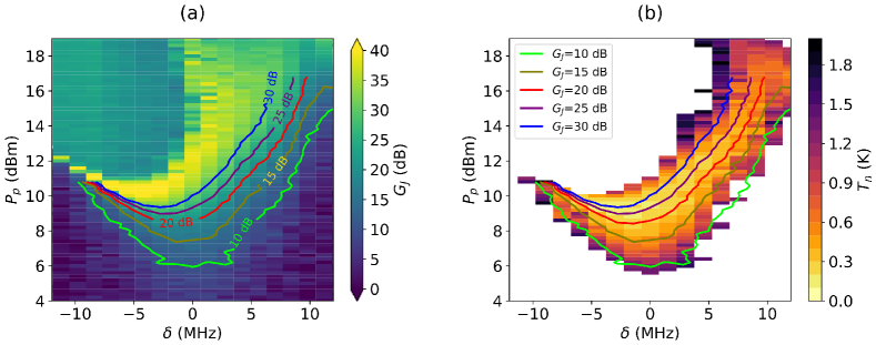
Figure 1: Measurements performed on a test bench setup. (a) $G_{J}$ as a function of $\delta$ and $P_{p}$. The overlaid lines correspond to contours calculated from the same data with the upper sections avoided for clarity. (b) $T_{n}$ as a function of $\delta$ and $P_{p}$. The gain contours shown in (a) are overlaid for comparison. It can be seen that noise temperatures along a particular equigain curve are minimal at the lowest $P_{p}$.

Table 1: A small section from a LUT constructed with the method described in this work. The colored rows correspond to points contributed from measurements shown in Fig. 2.

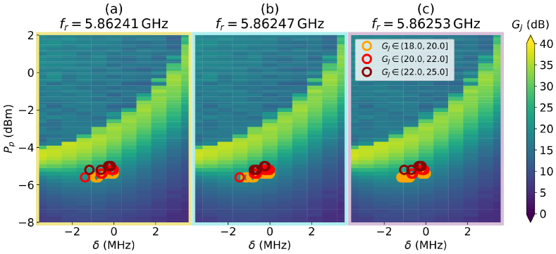
Figure 2: $G_{J}$ as a function of $\delta=f_{p}/2-f_{r}$ and $P_{p}$ performed at three example $i_{b}$ corresponding to $f_{r}=$5.862\,41\text{\,}\mathrm{GHz}$$ (a), $f_{r}=$5.862\,47\text{\,}\mathrm{GHz}$$ (b) and $f_{r}=$5.862\,53\text{\,}\mathrm{GHz}$$ (c). In a typical dataset there are a total of 341 such measurements. The circles correspond to the points chosen by the algorithm for inclusion in the LUT.

3 Application

The described procedure is implemented as part of an axion haloscope in the Center for Axion and Precision Physics Research (CAPP). The haloscope consists of a microwave cavity, an $8\text{\,}\mathrm{T}$ superconducting magnet surrounding it, and a receiver chain to transfer the signal into the spectrum analyzer. The experiment is housed in a Bluefors LD400 dilution refrigerator with the cavity and the JPA installed at the mixing-chamber (MC) plate. The MC temperature was kept at $40\text{\,}\mathrm{mK}$ during all of the experiments.

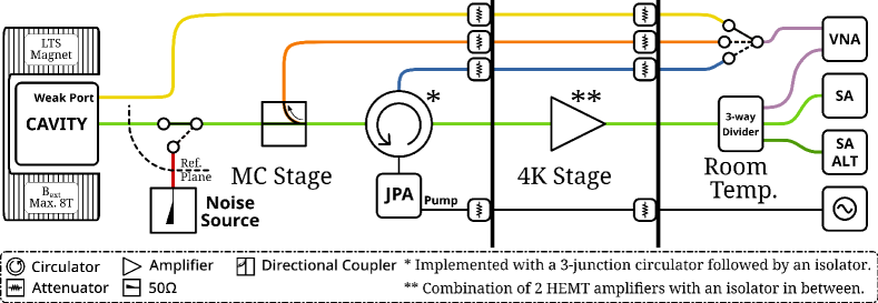
Figure 3: Simplified diagram for an axion haloscope. The colors are used to highlight several experimentally relevant signal paths. The JPA characterization measurements are performed with the room temperature switch pointing at the path shown in orange.

The $G_{J}$ is estimated by measuring $s_{21}$ at a single frequency $f=f_{sc}+$1\text{\,}\mathrm{kHz}$$ using a vector network analyzer (see Fig. 3). First, a baseline measurement ($s_{\mathrm{off}}$) is performed after tuning $f_{r}$ away from the frequency region of interest. Then the JPA is tuned to the desired working point, and a subsequent s-parameter measurement ($s_{\mathrm{off}}$) is performed. From these two measurements, the power gain is estimated via $G_{J}=10\log_{10}\left|{s_{\mathrm{on}}}/{s_{\mathrm{off}}}\right|^{2}$. Following the procedure described in the previous section, the swept data set for $G_{J}$ is obtained for $f_{r}$ in the range $5.85.96\text{\,}\mathrm{GHz}$. The LUT is generated using this data set with $f_{step}=$10\text{\,}\mathrm{kHz}$$ and $S_{G}=\{18,20,22,25\}$. The JPA tuning is then performed as part of the haloscope experiment following the steps below at each iteration: :

1. Tune the cavity to target frequency $f_{cav}$.

2. Let $f_{sc}$ to be $f_{cav}$.

3. Search the LUT for an entry corresponding to the chosen $f_{sc}$ and $G_{J}=$20\text{\,}\mathrm{dB}$$. If there is an entry, use the corresponding $(i_{b},f_{p},P_{p})$ to set the working point. If there is no entry, abort the procedure.

4. The impedance seen by the JPA will be slightly different depending on the cryogenic switch position. Since the LUT is generated with the switch pointing at the noise source, the $G_{J}$ measured at this step will usually be off by about $12\text{\,}\mathrm{dB}$. To compensate, fine-tune $P_{p}$ until $G_{J}$ is $20\pm 0.4\text{\,}\mathrm{dB}$. This will also correct for the small drifts in the pump signal power.

5. Measure the noise temperature.

6. Integrate axion-sensitive spectra.

In addition to in-situ measurements, noise temperatures of selected points from the LUT were also measured with the cryogenic switch pointing at the noise source (see Fig. 4).

4 Conclusion

For a JPA based detection chain, the $T_{n}$ and $G_{J}$ depend on the control parameters in a non-trivial manner. While it is possible to minimize $T_{n}$ at a given $G_{J}$ by adjusting the JPA control parameters during the experiment, this is time-consuming and tedious when the number of working points required is large. In this work, we proposed a look-up table based method for optimizing the noise temperature of a JPA at a given gain and operating frequency. In order to generate a viable LUT, a straightforward characterization protocol for gain measurements was used. The construction of the LUT relies on the knowledge that the $T_{n}$ is minimized with $P_{p}$ which was confirmed by separate measurements. The proposed approach was applied successfully in the context of an axion haloscope experiment around $5.9\text{\,}\mathrm{GHz}$. The LUT generation protocol was fully automated with a typical measurement time of about 12 hours for $120\text{\,}\mathrm{MHz}$ of coverage. The produced LUT is then viable for the whole duration of a cooldown which typically lasted more than a month. During the axion experiment, the JPA center frequency was tuned from $5.835.94\text{\,}\mathrm{GHz}$ using $20\text{\,}\mathrm{kHz}$ steps while maintaining minimal noise temperature. The tuning times were nominally less than $2\text{\,}\mathrm{s}$ with the limiting factor being the time cost of measurements during online gain correction. Moreover, it was observed that LUTs constructed on separate cooldowns of the cryostat yielded nearly identical results in noise temperature. Currently, this method is employed in all experiments involving a JPA in CAPP.

5 Acknowledgement

This work is supported in part by the Institute for Basic Science (IBS-R017-D1) and JST ERATO (Grant No. JPMJER1601). Arjan F. van Loo was supported by a JSPS postdoctoral fellowship.

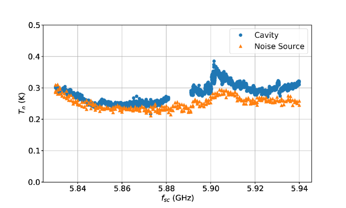
Figure 4: $T_{n}$ versus operating frequency ($f_{sc}$) for the detection chain in the axion experiment. Blue data points correspond to combined results of in-situ measurements during data taking runs spanning 6 months. The orange data set was measured within a day while the cryogenic switch is pointing at a $50\text{\,}\mathrm{\SIUnitSymbolOhm}$ resistor at $40\text{\,}\mathrm{mK}$ (noise source). The major source of difference between the two measurements is related to the non-ideal behavior of circulators leading to complex interactions between the cavity and the JPA. The noise temperature being higher than the quantum limit of $140\text{\,}\mathrm{mK}$ is attributed to the accumulated loss and reflection effects of the components before the JPA with the approximate contribution of $2026\text{\,}\mathrm{mK}$ from the later amplification stages.

References

- [1] C. Caves, Phys. Rev. D 26, 1817 (1982)
- [2] L. Zhong, E. Menzel, R. Di Candia, et al., New Journal Of Physics 15, 125013 (2013)
- [3] A. Clerk, M. Devoret, S. Girvin, et al., Rev. Mod. Phys. 82, 1155 (2010)
- [4] B. Brubaker, L. Zhong, Y. Gurevich, et al., Phys. Rev. Lett. 118, 061302 (2017)
- [5] S. Lee, S. Ahn, J. Choi, et al., Phys. Rev. Lett. 124, 101802 (2020)
- [6] J. Jeong, S. Youn, S. Bae, et al., Phys. Rev. Lett. 125, 221302 (2020)
- [7] O. Kwon, D. Lee, W. Chung, et al., Phys. Rev. Lett. 126, 191802 (2021)
- [8] Ç. Kutlu, A. F. van Loo, S. V. Uchaikin, et al., Supercond. Sci. Technol. 34, 085013 (2021).
- [9] T. Yamamoto, K. Inomata, M. Watanabe, et al., Appl. Phys. Lett. 93, 042510 (2008)
- [10] A. Roy, M. Devoret, Comptes Rendus Physique 17, 740 (2016)