Slow Kill for Big Data Learning

Abstract

Big-data applications often involve a vast number of observations and features, creating new challenges for variable selection and parameter estimation. This paper presents a novel technique called “slow kill,” which utilizes nonconvex constrained optimization, adaptive $\ell_{2}$-shrinkage, and increasing learning rates. The fact that the problem size can decrease during the slow kill iterations makes it particularly effective for large-scale variable screening. The interaction between statistics and optimization provides valuable insights into controlling quantiles, stepsize, and shrinkage parameters in order to relax the regularity conditions required to achieve the desired level of statistical accuracy. Experimental results on real and synthetic data show that slow kill outperforms state-of-the-art algorithms in various situations while being computationally efficient for large-scale data.

I Introduction

This paper studies how to build a parsimonious and predictive model in big data applications, where both the number of predictors and the number of observations can be extremely large. Let $y\in\mathbb{R}^{n}$ be a response vector with $n$ samples and $X=[x_{1},\ldots,x_{p}]\in\mathbb{R}^{n\times p}$ be a design matrix consisting of $p$ features or predictors. Consider a general learning problem with loss $l_{0}(X\beta;y)$ to measure the discrepancy between $X\beta$ and $y$. As $p$ can be much larger than $n$, a sparsity-promoting regularizer is often used to capture model parsimony

$$\min_{\beta\in\mathbb{R}^{p}}l_{0}(X\beta;y)+P(\beta;\lambda),$$ (1)

where $\lambda$ is a regularization parameter. There are numerous options for $l_{0}$ and $P$, neither of which are necessarily convex. In many cases, $l_{0}$ may be a negative log-likelihood function, but we will consider a more general setup that may not be based on likelihood.

Over the past decade, there have been significant advancements in statistical theory for the minimizers of the penalized problem (1). However, modern scientists often encounter challenges with big data, making it impractical to obtain globally optimal estimators even when convexity is present. This paper aims to incorporate computational considerations into statistical modeling, resulting in a new big-data learning framework with theoretical guarantees. When tackling these challenges in large-scale variable selection, the desired algorithms should possess the following traits:

(a) Ease in tuning. It is common in practice to seek a solution with a prescribed cardinality (or a specific number of variable, denoted by $q$). However, using an algorithm designed for the penalized problem (1) may require excessive computation, and the regularization parameter $\lambda$ may not be as intuitive when attempting to achieve this objective. Many practitioners perform a grid search for $\lambda$. However, when dealing with big data, the grid must be fine enough to encompass potentially useful candidate models, resulting in a substantial computational burden.

(b) Scalability. In addition to being efficient, an ideal algorithm should be easy to implement. Since ad-hoc procedures can be unreliable, it is preferable to employ an algorithm based on optimization rather than relying on heuristics. It would also be advantageous if the algorithm could adapt its parameters according to the available computational resources, which necessitates an understanding of the algorithm’s iteration complexity and per-iteration cost.

(c) Statistical guarantee. It is widely recognized that the lasso is effective for variable selection when the design matrix exhibits low coherence and the signal is sufficiently strong [1, 2]. Some simpler and faster methods, such as those for variable screening [3], are based on the assumption of independent (or only mildly correlated) features. While these weak-correlation assumptions allow for aggressive feature elimination, they are often restrictive for real-world high-dimensional data. Evaluating a globally optimal solution to (1) with an $\ell_{0}$-type penalty [4] does have a statistically sound guarantee regardless of coherence, but is only computationally feasible for small datasets. Therefore, a more pressing challenge is to design an iterative process that can relax the stringent regularity conditions required for attaining optimal statistical accuracy.

This work proposes a new approach called slow kill to tackle the aforementioned challenges. The main features of the algorithm are as follows.

• Interestingly, slow kill works in the opposite direction of forward pathwise methods and boosting algorithms, which all build up a model from the null [5, 6, 7, 8, 9].

• Slow kill incorporates adaptive $\ell_{2}$-shrinkage and growing learning rates to handle coherent designs and reduce computational burden. Its roots in optimization make it computationally scalable and easy to tune parameters.

• Theoretically, slow kill enjoys rigorous, provable guarantees of accuracy and linear convergence in a statistical sense. In particular, our theory supports backward quantile control and fast learning.

The rest of the paper is organized as follows. Section II investigates a hybrid regularized estimation in the regression setting to motivate some basic elements of slow kill and compares it to related works. Section III introduces the general slow kill procedure for a differentiable loss function and analyzes how the statistical error changes as the cycles progress. Section IV performs extensive simulations and real data experiments to compare slow kill to some state-of-the-art methods in terms of both efficiency and accuracy. We summarize our findings in Section V. More technical details are provided in the appendix.

Notations and symbols. The following notations and symbols will be used. Let $[n]=\{1,\ldots,n\}$ and $\lfloor x\rfloor$ be the largest integer smaller than or equal to $x$. Define $a\vee b=\max(a,b)$ and $a\wedge b=\min(a,b)$. We use $a\lesssim b$ to denote $a\leq cb$ for some positive constant $c$, and the constants denoted by $c$ or $C$ may not be the same at each occurrence. Given any $\beta\in\mathbb{R}^{p}$, we use $\mathcal{J}(\beta)\subset[p]$ to denote its support, i.e., $\mathcal{J}(\beta)=\{j:\beta_{j}\neq 0\}$, and $J(\beta)=|\mathcal{J}(\beta)|=\|\beta\|_{0}=\sum_{j=1}^{p}1_{\beta_{j}\neq 0}$. Given $I\subset[p]$, we use $X_{I}$ to denote the sub-matrix of $X$ formed with the columns in $I$, and $\beta_{I}$ the subvector associated with $I$. In particular, $x_{j}$ denotes the $j$th column of $X$ for any $j\in[p]$. When $A$ is a symmetric matrix, we use $A_{I}$ to denote the sub-matrix of $A$ formed with the columns and rows indexed by $I$, and $\lambda_{\max}(A)$, $\lambda_{\min}(A)$ to denote its largest and smallest eigenvalues, respectively.

Given $X\in\mathbb{R}^{n\times p}$, the restricted isometry numbers $\rho_{+}(s)$, $\rho_{-}(s)$ [10] are the smallest and largest numbers, respectively, that satisfy

$$\rho_{-}(s)\|\beta\|_{2}^{2}\leq\|X\beta\|_{2}^{2}\leq\rho_{+}(s)\|\beta\|_{2}^{2},\ \forall\beta\in\mathbb{R}^{p}:\|\beta\|_{0}\leq s,$$ (2)

and their dependence on $X$ is omitted. Obviously, $0\leq\rho_{-}(s)\leq\rho_{+}(s)\leq\rho_{+}(p)=\|X\|_{2}^{2}$, where $\|X\|_{2}$ denotes the spectral norm of $X$.

For ease of presentation, we introduce a quantile-thresholding operator $\Theta^{\#}$ which performs simultaneous thresholding and $\ell_{2}$-shrinkage [11]. Given any $s=[s_{1},\ldots,s_{p}]^{T}\in\mathbb{R}^{p}$, $\Theta^{\#}(s;q,\eta)=[t_{1},\ldots,t_{p}]^{T}$ satisfying $t_{(j)}=s_{(j)}/(1+\eta)\mbox{ if }1\leq j\leq q\mbox{, and }0\mbox{ otherwise,}$ where $s_{(1)},\ldots,s_{(p)}$ are the order statistics of $s_{1},\ldots,s_{p}$ satisfying $|s_{(1)}|\geq\cdots\geq|s_{(p)}|$, and $t_{(1)},\ldots,t_{(p)}$ are defined similarly. To avoid ambiguity, we make a $\Theta^{\#}$-uniqueness assumption in performing $\Theta^{\#}(s;q,\eta)$ throughout the paper: either $|s_{(q)}|>|s_{(q+1)}|$ or $s_{(q)}=s_{(q+1)}=0$ occurs. The multivariate quantile thresholding function $\vec{\Theta}^{\#}(S;{q},\eta)$ for any $S=[s_{1},\ldots,s_{p}]^{T}\in\mathbb{R}^{p\times m}$ is defined as a $p\times m$ matrix ${T}=[{t}_{1},\ldots,{t}_{p}]^{T}$ with ${{t}}_{j}=s_{j}/(1+\eta)$ if $\|s_{j}\|_{2}$ is among the ${q}$ largest elements in $\{\|s_{j}\|_{2}:1\leq s\leq p\}$, and ${0}$ otherwise.

II Why Backward Selection?

This section is to motivate a “top-down” algorithm design in the fundamental regression setting. The quadratic loss is an important case of strongly convex losses and examining this case will provide a foundation for more general studies under restricted strong convexity.

Assume $y=X\beta^{*}+\epsilon$, where $\beta^{*}\in\mathbb{R}^{p}$, $\|\beta^{*}\|_{0}\leq s$ with $s\leq p\wedge n$. To begin with, we consider an $\ell_{0}$-constrained, $\ell_{2}$-penalized optimization problem to estimate the coefficient vector in high dimensions,

$$\min_{\beta}\frac{1}{2}\|y-X\beta\|_{2}^{2}+\frac{\eta_{0}}{2}\|\beta\|_{2}^{2}\equiv f(\beta)\mbox{\; s.t. }\|\beta\|_{0}\leq q.$$ (3)

When $X,y$ are not centered, an intercept term ${1}\alpha$ should be added in the loss, and $\alpha$ is subject to no regularization. The hybrid regularization in (1) differs from the commonly used linear combination of $\ell_{1}$ and $\ell_{2}$ penalties in the elastic net [12]. Compared to the regular $\ell_{1}$ penalty and other nonconvex penalties, $\|\cdot\|_{0}$ is arguably an ideal choice for enforcing sparsity and does not incur any unwanted bias. The constraint parameter $q\,(\leq p)$ directly controls the number of variables in the resulting model, making it more convenient to use than a penalty parameter $\lambda$. The simultaneous $\ell_{2}$-penalty is to compensate for collinearity and large noise, and is later used to overcome some obstacles in backward elimination. The associated regularization parameter $\eta_{0}$ can be easily tuned and is not highly sensitive in experiments. Our theoretical analysis will reveal the benefits of a carefully designed shrinkage sequence for both numerical stability and statistical accuracy.

Problem (3) is nonconvex and includes a discrete constraint. While it can be challenging to computationally solve problems of this nature, it is possible to find a local minimum using a scalable iterative optimization algorithm. Moreover, in the era of big data, it may not be necessary to fully solve (3) in order to achieve good statistical performance for “regular” problems and analyzing algorithm-driven non-global estimators is crucial to discovering new and cost-effective methods for improving the statistical performance of nonconvex optimization. Concretely, to introduce a prototype algorithm, we first construct a surrogate function $g(\beta,\beta^{-})$ for (3),

$$\begin{split}g(\beta,\beta^{-})=\frac{1}{2}\lVert y-X\beta^{-}\rVert_{2}^{2}+\langle X^{T}(X\beta^{-}-y),\beta-\beta^{-}\rangle+\frac{\rho}{2}\lVert\beta-\beta^{-}\rVert_{2}^{2}+\frac{\eta_{0}}{2}\lVert\beta\rVert_{2}^{2},\end{split}$$

with $\rho>0$ to be chosen later, and then define a sequence of iterates by

$$\beta^{(t+1)}=\arg\min_{\beta:\|\beta\|_{0}\leq q}g(\beta,\beta^{(t)}).$$ (4)

Recall the quantile-thresholding operator $\Theta^{\#}$ defined at the end of Section I. With some simple algebra (details omitted), we obtain an iterative quantile-thresholding algorithm

$$\beta^{(t+1)}=\Theta^{\#}\Big{\{}\beta^{(t)}-\frac{1}{\rho}X^{T}(X\beta^{(t)}-y);q,\frac{\eta_{0}}{\rho}\Big{\}}.$$ (5)

The first step amounts to the sure independence screening [3] when $\beta^{(0)}={0}$. However, (5) iterates to lessen greediness with a low per-iteration cost.

The update rule in (5) possesses some desirable computational properties. For instance, if $\rho$ is large enough (more specifically, $\rho\geq\rho_{+}(2q)$ with $\rho_{+}(\cdot)$ defined in (2)), then the algorithm shows a worst-case sublinear convergence rate, regardless of the problem’s dimensions, coherence, and signal strength. The obtained solutions (though not necessarily optimal) can be characterized as fixed points of the algorithm mapping defined in (4). For more results and technical details, please refer to Theorem A.1.

This class of procedures has been used in signal and information processing [11, 13], and in the special case of $\eta_{0}=0$, the plain update rule of (5) falls under the category of iterative hard-thresholding (IHT) algorithms [14, 15] which only exhibit mediocre performance (cf. Remark 3 and Section IV). In fact, there is much potential for improvement by adaptively adjusting the three key parameters $\rho,\eta_{0},q$ in (5), which has not been systematically explored in the literature.

II-A Statistical error analysis: power and limitations

While optimization error is important for analyzing an algorithm, our main focus is on statistical error. This subsection investigates the prototype algorithm (5) to motivate new techniques in later sections. In order to obtain sharp nonasymptotic results for this algorithm, it is important to note that the thresholds vary from iteration to iteration and the final estimator may not be globally optimal.

Recall $y=X\beta^{*}+\epsilon$ with $\|\beta^{*}\|_{0}\leq s$. Let

$$\vartheta:=q/s$$

with $\vartheta>1$ throughout the paper. A fixed point $\hat{\beta}$ associated with (5) that satisfies the following equation is called a $\Theta^{\#}$-estimator,

$$\hat{\beta}=\Theta^{\#}\big{\{}\hat{\beta}-\frac{1}{\rho}X^{T}(X\hat{\beta}-y);q,\bar{\eta}_{0}\big{\}},\ \mbox{with}\ \bar{\eta}_{0}=\eta_{0}/\rho.$$ (6)

Theorem 1 studies the statistical accuracy of these estimators.

Theorem 1.

Assume that $\epsilon$ is a sub-Gaussian random vector with mean zero and scale bounded by $\sigma$ (cf. Definition A.1 in the appendix). Let $\hat{\beta}$ be any estimator satisfying (6) for some $\eta_{0}\geq 0$ with $\|\hat{\beta}\|_{0}=q$, and $\rho>0$ be chosen such that

$$\begin{split}\frac{\rho-\{(2-\varepsilon)\sqrt{\vartheta}-1\}\eta_{0}}{\sqrt{\vartheta}}\|\beta\|_{2}^{2}\leq(2-\delta)\|X\beta\|_{2}^{2}\quad\forall\beta:\|\beta\|_{0}\leq(1+\vartheta)s\end{split}$$ (7)

for some $\varepsilon,\delta>0$. Then with probability at least $1-Cp^{-c},$

$$\|X(\hat{\beta}-\beta^{*})\|_{2}^{2}\vee\frac{\eta_{0}\varepsilon}{\delta}\|\hat{\beta}-\beta^{*}\|_{2}^{2}\lesssim\frac{1}{\delta^{2}}\sigma^{2}\vartheta s\log{\frac{ep}{\vartheta s}}+\frac{\eta_{0}}{\delta\varepsilon}\|\beta^{*}\|_{2}^{2},$$ (8)

where $C,c>0$ are constants.

From the error bound, (5) can achieve the minimax optimal error rate of $\mathcal{O}(\sigma^{2}s\log(ep/s))$ [16], under the assumption of (7) and when $\vartheta,\delta,\varepsilon$ are treated as constants. The result does not need $\eta_{0}$ to be exactly zero. In fact, a positive $\eta_{0}$ can actually be beneficial in satisfying the condition of (7) (e.g., $\rho=(1.9\sqrt{\vartheta}-1)\eta_{0}+1.9\sqrt{\vartheta}\rho_{-}(q+s)$ and $\varepsilon=\delta=0.1$, applicable to $q>n$). Another interesting observation is that $\rho$ should be chosen to be properly small to achieve good statistical accuracy, which is in contrasts to the bound $\rho\geq\rho_{+}(2q)$ mentioned earlier for numerical convergence. The remarks below make some further extensions and comparisons.

Remark 1 (Estimation error bounds and faithful variable selection).

The $\ell_{2}$-recovery result of Theorem 1 is fundamental, and can be used to derive estimation error bounds in other norms under proper regularity conditions.

Theorem 2.

In the setup of Theorem 1, suppose the regularity condition (7) is replaced by

$$\begin{split}\big{\{}\frac{\rho-(2\sqrt{\vartheta}-1)\eta_{0}}{\sqrt{\vartheta}}+\delta\rho_{+}((1+\vartheta)s)\big{\}}\|\beta\|_{2}^{2}\leq 2\|X\beta\|_{2}^{2},\ \forall\beta:\|\beta\|_{0}\leq(1+\vartheta)s\end{split}$$ (9)

for some $\delta>0$. Then

$$\|\hat{\beta}-\beta^{*}\|_{2}^{2}\lesssim\frac{1}{\delta^{2}\rho_{+}((1+\vartheta)s)}\sigma^{2}\vartheta s\log{\frac{ep}{\vartheta s}}+\frac{\eta_{0}^{2}}{\delta^{2}\rho_{+}((1+\vartheta)s)}\|\beta^{*}\|_{2}^{2}$$ (10)

holds with probability at least $1-Cp^{-c}$, for some $C,c>0$. Moreover, under

$$\nu\|\beta\|_{\infty}\leq\|(X^{T}X+\eta_{0}I)\beta\|_{\infty}/n,\ \ \beta:\|\beta\|_{0}\leq(1+\vartheta)s$$ (11)

for some $\nu>0$, any fixed-point $\hat{\beta}$ satisfies

$$\|\hat{\beta}-\beta^{*}\|_{\infty}\leq\frac{(\rho+\eta_{0})}{n\nu\sqrt{\vartheta-1}}\frac{\|\hat{\beta}-\beta^{*}\|_{2}}{\sqrt{s}}+\frac{\|X^{T}\epsilon\|_{\infty}}{n\nu}+\frac{\eta_{0}}{n\nu}\|\beta^{*}\|_{\infty,}$$ (12)

and

$$\|(\hat{\beta}-\beta^{*})_{\mathcal{J}^{*}}\|_{\infty}+(1-\frac{\rho+\eta_{0}}{n\nu})\|(\hat{\beta}-\beta^{*})_{\hat{\mathcal{J}}\setminus\mathcal{J}^{*}}\|_{\infty}\leq\frac{\|X^{T}\epsilon\|_{\infty}}{n\nu}+\frac{\eta_{0}}{n\nu}\|\beta^{*}\|_{\infty},$$ (13)

where $\mathcal{J}^{*}=\mathcal{J}(\beta^{*})$, $\hat{\mathcal{J}}=\mathcal{J}(\hat{\beta})$.

Compared with (7), the condition of (9) replaces $\delta\|X\beta\|_{2}^{2}$ by $\delta\rho_{+}((1+\vartheta)s)\|\beta\|_{2}^{2}$. When $q$ and $s$ are small, $\rho_{+}((1+\vartheta)s)$ is of the order $\mathcal{O}(n)$. Therefore, (10) becomes $\|\hat{\beta}-\beta^{*}\|_{2}^{2}\lesssim\{\sigma^{2}s\log(ep/s)\}/{n},$ assuming $\delta,\vartheta$ are constants and $\eta_{0}$ is properly small.

Moreover, the element-wise error bound (12) implies faithful variable selection under regularity condition (11) (which, like previous regularity conditions, favors low coherence, i.e., the off-diagonal entries of $X^{T}X/n$ should be relatively small in magnitude). Specifically, assuming $\vartheta,\nu,\delta$ are constants, $\|x_{j}\|_{2}\lesssim\sqrt{n}$, $\rho+\eta_{0}\lesssim n$ and the beta-min condition $\min_{j\in\mathcal{J}^{*}}|\beta^{*}_{j}|>c\sigma\{\log(ep)/{n}\}^{1/2}$ with a sufficient large constant $c$, (12) indicates that the $s$ largest elements in $|\hat{\beta}_{j}|$ correspond to $\mathcal{J}^{*}=\{j:\beta^{*}_{j}\neq 0\}$ with high probability.

Remark 2 (Fixed points vs. globally optimal solutions).

The statistical accuracy results (8), (10), and (12) are proved for all nonglobal fixed-point estimators defined by (6). Our proof can be slightly modified to show that if a globally optimal solution can be computed, the statistical error rate remains unchanged but the left-hand side of (7) becomes 0, indicating that the regularity condition always holds for any $\delta\leq 2$. However, relying on multiple starting points to obtain a globally optimal solution and thus improve statistical performance can be inefficient for large datasets.

Remark 3 (Comparison with some theoretical works).

The aforementioned class of IHT algorithms may refer to the use of hard-thresholding $\Theta_{H}({s};\lambda)=[s_{i}1_{|s_{i}|\geq\lambda}]$ with a fixed threshold $\lambda$, or a varying threshold as the $q/p$-th quantile of $|s_{i}|$ ($1\leq i\leq p$) by fixing $q$ [14, 15]. In comparison, the $\ell_{2}$ component in (5) should not be ignored, and it may result in a different sparsity pattern in the presence of high coherence and large $p$. Fairly speaking, the performance of IHT is not on par with some standard statistical methods and packages (such as the lasso). This is why we performed theoretical analysis in the hopes of discovering and developing new techniques.

In a theoretical study, [17] obtained a convergence result in terms of function value under

$$\vartheta>\rho_{+}^{2}(2q)/\rho_{-}^{2}(2q),$$

which improves the condition in [18]

$$\vartheta>32\rho_{+}^{2}(2q)/\rho_{-}^{2}(2q).$$

Our condition in Theorem 1 is even less restrictive. For example, a sufficient condition for (7) is

$$\vartheta>\{\rho_{+}(2q)+\eta_{0}\}^{2}/[4\{\rho_{-}(q+s)+\eta_{0}\}^{2}],$$

or

$$\vartheta>\{\rho_{+}(2q)+\eta_{0}\}^{2}/[4\{\rho_{-}(2q)+\eta_{0}\}^{2})]$$

since $\rho_{-}(q+s)\geq\rho_{-}(2q)$, which becomes $\vartheta>\rho_{+}^{2}(2q)/\{4\rho_{-}^{2}(2q)\}$ in the worst case of $\eta_{0}=0$. In conclusion, $32\rho_{+}^{2}(2q)/\rho_{-}^{2}(2q)\geq\rho_{+}^{2}(2q)/\rho_{-}^{2}(2q)\geq\rho_{+}^{2}(2q)/\{4\rho_{-}^{2}(2q)\}\geq\rho_{+}^{2}(2q)/[4\{\rho_{-}(q+s)\}^{2}]\geq\{\rho_{+}(2q)+\eta_{0}\}^{2}/[4\{\rho_{-}(q+s)+\eta_{0}\}^{2}]$, and our obtained error rate of $\sigma^{2}s\log(ep/s)$ is minimax optimal.

Interested readers may also refer to [19, 20, 21, 9, 17, 22], for example, for the analyses of various penalties and mixed thresholding rules, with an error rate of $\sigma^{2}s\log(ep)$. Since our purpose is to design a new backward selection algorithm for problems with a predetermined number of features, we will not discuss their technical assumptions. The experiments in Section IV make a comprehensive comparison of different methods in various scenarios.

II-B New means of improvement for large-scale data

Providing provable guarantees for prediction, estimation, and variable selection is reassuring. But the real challenge lies in finding innovative techniques that can relax the required regularity conditions to ensure good statistical accuracy, while being more cost-effective than using multiple random starts. To gain further insights, we can use the restricted isometry numbers (as defined in (2)) to provide a sufficient condition for (7):

$$\rho<2\sqrt{\vartheta}\rho_{-}(q+s)+(2\sqrt{\vartheta}-1)\eta_{0}\mbox{\ \ or \ }4\vartheta>\frac{(\rho+\eta_{0})^{2}}{(\rho_{-}(q+s)+\eta_{0})^{2}}.$$ (14)

II-B1 “Fast” learning

One key takeaway from the results presented in Section II-A is the importance of the inverse learning rate, $\rho$. In the field of machine learning, it is commonly advised to use a “slow” learning rate when training a nonconvex model. This can ensure good computational performance, as evidenced by the lower bound of $\rho$ in Theorem A.1. However, it is important to note that according to (14), using an excessively large value for $\rho$ may compromise the statistical guarantee of the model.

In fact, (7) suggests that smaller values of $\rho$ are preferred, and combining statistical and numerical analysis leads to the following range for $\rho$:

$$\rho_{+}(2q)\leq\rho\leq 2\sqrt{\vartheta}\rho_{-}(q+s)+(2\sqrt{\vartheta}-1)\eta_{0}.$$ (15)

In convex programming, the choice of stepsize does not affect the optimality of the solution as long as the algorithm converges. However, in our case of nonconvex constrained optimization, it is important to choose a large enough value for $1/\rho$ not only to gain fast convergence, but also to ensure statistical accuracy. To the best of our knowledge, this is a novel finding. Since it may not be easy to determine the theoretical restricted isometry numbers in practice, a routine line search for the step size can be used. Specifically, according to the proof in Appendix A-A, one can use the majorization condition $f(\beta^{(t+1)})\leq g(\beta^{(t+1)},\beta^{(t)})\mbox{ or }\|X(\beta^{(t+1)}-\beta^{(t)})\|_{2}^{2}\leq\rho\|\beta^{(t+1)}-\beta^{(t)}\|_{2}^{2}$ to prevent $\rho$ from becoming too large while still preserving the convergence properties stated in Theorem A.1. The concept of using an iteration-varying sequence $\rho_{t}$ will be important in the next section.

II-B2 “Backward” selection

Another important discovery is the influence of cardinality control. If we use a conservative inverse learning rate of $\rho=\rho_{+}(2q)$, then (14) imposes a limit on the restricted condition number of the design matrix:

$$\vartheta>[\rho_{+}(2q)+\eta_{0}]^{2}/\{4[\rho_{-}(q+s)+\eta_{0}]^{2})\}.$$ (16)

This suggests a promising approach to relax the regularity condition by increasing the value of $\vartheta$.

Figure 1 confirms the point assuming random designs: the larger the value of $q$ is, the more likely it is for (14) to hold on large-scale data. Random matrix theory also supports this idea.

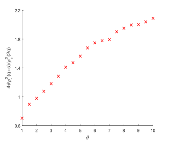
Figure 1: An illustration of how $4\vartheta\rho_{-}^{2}(q+s)/\rho_{+}^{2}(2q)$ varies as $\vartheta$ increases. Here, the rows of $X$ are independently drawn from a multivariate Gaussian distribution with zero mean and the covariance $\Sigma=[0.5^{|i-j|}]$, $n=2\mbox{,}000,p=4\mbox{,}000,s=4$. To determine $\rho_{\pm}$ for a given matrix $X$, we perform a random sampling. The results are averaged over 100 independent $X$’s that are generated from the same distribution.

Theorem 3.

Assume that the rows of the random matrix $X\in\mathbb{R}^{n\times p}$ are independent and identically distributed as $N({0},\Sigma)$, where $\Sigma_{ii}\leq 1$. Let $\lambda^{(2q)}_{\max}$ be the largest eigenvalue of $\Sigma_{I}$ for all $I\subset[p]$ with $|I|\leq 2q$, and $\lambda^{(q+s)}_{\min}$ be the smallest eigenvalue of $\Sigma_{I}$ for all $I\subset[p]$ with $|I|\leq q+s$. Then for any $0<c<1$,

$$\frac{\rho_{+}(2q)}{\rho_{-}(q+s)}\leq\left\{\frac{(1+c)\sqrt{\lambda^{(2q)}_{\max}}+\sqrt{\{2\lambda^{(2q)}_{\max}q\log(ep/q)\}/n}+\sqrt{2q/n}}{(1-c)\sqrt{\lambda^{(q+s)}_{\min}}-\sqrt{\{\lambda^{(q+s)}_{\min}(q+s)\log(ep/q)\}/n}-\sqrt{(q+s)/n}}\right\}^{2}$$ (17)

with probability at least $1-2\exp(-nc^{2}/2)$, assuming $n\geq\{2(q+s)/(1-c)^{2}\}\{1/\lambda^{(q+s)}_{\min}+\log(ep/q)\}$.

The results can be extended to sub-Gaussian designs (by using, for example, Theorem 6.2 of [23] and Weyl’s theorem). Let us consider the Toeplitz design $\Sigma=[\tau^{|i-j|}]$ with $0\leq\tau<1$. By the interlacing theorem,

$$\begin{split}(1-\tau)/(1+\tau)=\lambda_{\min}(\Sigma)\leq\lambda^{(q+s)}_{\min}\leq\lambda^{(2q)}_{\max}\leq\lambda_{\max}(\Sigma)=(1+\tau)/(1-\tau),\end{split}$$

and so the right-hand side of (17) is bounded by a constant with high probability as $n\gg q\log{(ep/q)}$. Accordingly, the regularity condition can be satisfied with a properly large $\vartheta$.

Of course, the error bound in (8) also increases with larger values of $q$. To address this issue, we propose employing a decreasing sequence of $q_{t}$ to progressively tighten the cardinality constraint. Based on previous discussions, it is thus advisable to use increasing learning rates $1/\rho_{t}$ (such as $1/\rho_{+}(2q_{t})$) in the iterative process. It may also be beneficial to adjust the shrinkage parameter to a sequence $\eta_{t}$, particularly when $q_{t}>n$. This resulting algorithm, which combines progressive quantiles, $\ell_{2}$-shrinkage, and learning rates, will be referred to as “slow kill.” It differs from the pure optimization algorithm (5) with a fixed $q$ and from various bottom-up boosting and greedy algorithms that are commonly used in the literature.

The purpose of this section is to provide a compelling rationale for certain aspects of slow kill techniques. We will present results in a more general setting, including fast convergence of the iterates and how slow kill improves the quality of the initial estimate as $q_{t}$ approaches $q$, further relaxing the regularity conditions.

III Adaptive Control of Quantiles, Learning Rates, and $\ell_{2}$-shrinkage

Given a general loss, based on the discussions in the last section, we pursue sparsity in $\beta$ via

$$\min_{\beta\in\mathbb{R}^{p}}l_{0}(X\beta;y)+\frac{\eta_{0}}{2}\|\beta\|_{2}^{2}\,\equiv l(\beta)+\frac{\eta_{0}}{2}\|\beta\|_{2}^{2}\equiv f(\beta)\mbox{ s.t. }\lVert\beta\lVert_{0}\leq q,$$ (18)

where for notational ease, $l_{0}(X\beta;y)$ is often abbreviated as $l(\beta)$. Again, the use of hybrid regularization is intended to address collinearity and large $p$. We assume that the regularization parameters $q,\eta_{0}$ are given in the algorithm design and theoretical analysis. (Of course, given $q$, one can easily tune the value of $\eta_{0}$ using methods such as AIC; as for the selection of $q$, an information criterion is provided in the Appendix A-H.) The generalized Bregman function for a differentiable $l$ is one of the main tools we use to handle a variety of losses:

$${\mathbf{\Delta}}_{l}(\beta_{1},\beta_{2}):=l(\beta_{1})-l(\beta_{2})-\langle\nabla l(\beta_{2}),\beta_{1}-\beta_{2}\rangle,$$ (19)

where the differentiability can be replaced by directional differentiability to analyze a wide range of algorithms in statistical computation [22]. If $l$ is also strictly convex, ${\mathbf{\Delta}}_{l}$ becomes the standard Bregman divergence [24, 25]. When $l(\cdot)=\|\cdot\|_{2}^{2}/2$, ${\mathbf{\Delta}}_{l}(\beta_{1},\beta_{2})=\|\beta_{1}-\beta_{2}\|_{2}^{2}/2$, which is symmetric, and we abbreviate it to ${\mathbf{D}}_{2}(\beta_{1},\beta_{2})$. Define the symmetrized version of ${\mathbf{\Delta}}_{l}(\beta_{1},\beta_{2})$ by $\bar{\mathbf{\Delta}}_{l}(\beta_{1},\beta_{2}):=\{{\mathbf{\Delta}}_{l}(\beta_{1},\beta_{2})+\mathrel{\mathop{{\mathbf{\Delta}}}\limits^{\vbox to0.0pt{\kern-2.0pt\hbox{$\scriptstyle\smallsetminus$}\vss}}}_{l}(\beta_{1},\beta_{2})\}/2,$ where $\mathrel{\mathop{{\mathbf{\Delta}}}\limits^{\vbox to0.0pt{\kern-2.0pt\hbox{$\scriptstyle\smallsetminus$}\vss}}}_{l}(\beta_{1},\beta_{2})={\mathbf{\Delta}}_{l}(\beta_{2},\beta_{1})$. As an extension of (2), we introduce two generalized restricted isometry numbers $\rho_{+}^{l}(s_{1},s_{2})$, $\rho_{-}^{l}(s_{1},s_{2})$ that satisfy

$${\mathbf{\Delta}}_{l}(\beta_{1},\beta_{2})\leq\rho_{+}^{l}(s_{1},s_{2}){\mathbf{D}}_{2}(\beta_{1},\beta_{2}),\ \forall\beta_{i}:\|\beta_{i}\|_{0}\leq s_{i},i=1,2$$ (20)

$${\mathbf{\Delta}}_{l}(\beta_{1},\beta_{2})\geq\rho_{-}^{l}(s_{1},s_{2}){\mathbf{D}}_{2}(\beta_{1},\beta_{2}),\ \forall\beta_{i}:\|\beta_{i}\|_{0}\leq s_{i},i=1,2.$$ (21)

We differentiate $s_{1},s_{2}$ because ${\mathbf{\Delta}}_{l}$ may not be symmetric. These numbers will be convenient and useful for theoretical purposes; for example, Theorem 4 and Theorem 5 will use positive $\rho_{+}^{l}(q,q)$ and $\rho_{+}^{l}(q,s)$, respectively, while Theorem 6 will use nonnegative $\rho_{-}^{l}$. When $l(\beta)=\|X\beta-y\|_{2}^{2}/2$, ${\mathbf{\Delta}}_{l}(\beta_{1},\beta_{2})=\|X\beta_{1}-X\beta_{2}\|_{2}^{2}/2$ and $\rho^{l}_{+}(s_{1},s_{2})=\rho_{+}(s_{1}+s_{2})$. More generally, if the gradient of $l_{0}(\cdot;y)$ is $L$-Lipschitz continuous, as is the case in regression or logistic regression,

$$\|\nabla l_{0}(\xi_{1};y)-\nabla l_{0}(\xi_{2};y)\|_{2}\leq L\|\xi_{1}-\xi_{2}\|_{2},$$ (22)

for all $\xi_{1},\xi_{2}\in\mathbb{R}^{n}$, then it is easy to show that

$$\rho_{+}^{l}(s_{1},s_{2})\leq L\rho_{+}(s_{1}+s_{2})\ (\leq L\|X\|_{2}^{2}).$$ (23)

III-A Numerical convergence and statistical accuracy for the general optimization algorithm

First, we extend the previous iterative quantile-thresholding algorithm to handle losses that may not be quadratic. Construct the following surrogate function

$$g(\beta,\beta^{-})=l_{0}(X\beta;y)+\frac{\eta_{0}}{2}\|\beta\|_{2}^{2}+(\rho{\mathbf{D}}_{2}-{\mathbf{\Delta}}_{l})(\beta,\beta^{-}),$$ (24)

which is by linearizing the loss (only). Then, similar to the derivation in Section II, (24) leads to an algorithm

$$\beta^{(t+1)}=\Theta^{\#}\Big{\{}\beta^{(t)}-\frac{1}{\rho}X^{T}\nabla l_{0}(X\beta^{(t)};y);q,\frac{\eta_{0}}{\rho}\Big{\}}.$$ (25)

Some basic numerical properties are summarized as follows.

Theorem 4.

Assume that $\inf_{\xi,y}l_{0}(\xi;y)>-\infty$. Consider (25) starting from an arbitrary feasible $\beta^{(0)}$. Then $\rho\geq\rho_{+}^{l}(q,q)$ guarantees that for all $t\geq 0$, $f(\beta^{(t+1)})\leq g(\beta^{(t+1)},\beta^{(t)})$ and $(\rho-\rho_{+}^{l}(q,q)){\mathbf{D}}_{2}(\beta^{(t+1)},\beta^{(t)})\leq f(\beta^{(t)})-f(\beta^{(t+1)}),$ and so the objective function values converge as $t\to\infty$. Assume $\rho>\rho_{+}^{l}(q,q)$, $\eta_{0}>0$ and $\nabla l_{0}$ is continuous. Then every accumulation point $\hat{\beta}$ of $\beta^{(t)}$ satisfies the fixed-point equation

$$\hat{\beta}=\Theta^{\#}\{\hat{\beta}-X^{T}\nabla l_{0}(X\hat{\beta};y)/\rho;q,\eta_{0}/\rho\}.$$ (26)

Furthermore, if $l_{0}(\cdot;y)$ is convex, $\lim_{t\to\infty}\beta^{(t)}=\hat{\beta}$, and under $\|\hat{\beta}\|_{0}=q$, $\hat{\beta}$ is a local minimizer to problem (18) and the support of $\beta^{(t)}$ stabilizes in finitely many iterations.

Next, we turn to the statistical accuracy of the estimators that are defined by (26). To overcome the obstacle that the loss is not necessarily associated with a probability density function, we define the concept of effective noise with respect to the statistical truth $\beta^{*}$ as

$$\epsilon=-\nabla l_{0}(X\beta^{*};y),$$ (27)

where we treat $X$ as fixed and $y$ as random in this section. The definition of effective noise in (27) does not depend on the regularizer. In the special case of a generalized linear model with cumulant function $b$ and canonical link function $g=(b^{\prime})^{-1}$, the loss is $l(\beta)=l_{0}(X\beta;y)=-\langle y,X\beta\rangle+\langle 1,b(X\beta)\rangle$, and so $\epsilon=y-g^{-1}(X\beta^{*})=y-\,\mathbb{E}y$. For regression, the effective noise term $\epsilon$ is equivalent to the raw noise, which is usually assumed to be Gaussian. In the case of classification using the logistic deviance, $\epsilon$ is bounded, making it sub-Gaussian. In fact, any loss function with a bounded derivative, such as Huber’s loss, Hampel’s loss, or the hinge loss, will always result in a sub-Gaussian $\epsilon$, regardless of the distribution of $y$. In this section, we assume that the effective noise is a sub-Gaussian random vector with mean zero and scale bounded by $\sigma$. However, our proof techniques can be applied more generally. The following theorem provides a risk bound for the estimators obtained by (25), and also demonstrates the impact of the quality of the starting point on the regularity condition.

Theorem 5.

Let $\hat{\beta}:\|\hat{\beta}\|_{0}=q$ be an estimate obtained from (25) with a feasible starting point $\beta^{(0)}$, namely, $\hat{\beta}\in\min_{\|\beta\|_{0}\leq q}g(\beta,\hat{\beta})$ and $f(\hat{\beta})\leq f(\beta^{(0)})$ with $\|\beta^{(0)}\|_{0}\leq q$. Define

$${P_{o}(q)=q\log(ep/q).}$$ (28)

Suppose that $\beta^{(0)}$ satisfies

$$\begin{split}\,\mathbb{E}{\mathbf{D}}_{2}(\beta^{(0)},\beta^{*})=\mathcal{O}(M)\frac{\sigma^{2}P_{o}(q)+\sigma^{2}}{n}\mbox{ for some}\ \,M:1\leq M\leq+\infty.\end{split}$$ (29)

Let $Q=\{\rho_{+}(q+s)M/n\}^{1/2}+\{\rho_{+}^{l}(q,s)+\eta_{0}\}M/n$. Assume for some $\delta>0,0<\varepsilon\leq 1$ and large $K\geq 0$,

$$\begin{split}&K\sigma^{2}P_{o}(\vartheta s)+\Big{\{}2(1-\frac{1}{M})\bar{\mathbf{\Delta}}_{l_{0}}+\frac{C}{M(Q\delta\vee 1)}{\mathbf{\Delta}}_{l_{0}}-\delta{\mathbf{D}}_{2}\Big{\}}(X\beta,X\beta^{\prime})\\ &\,\geq\frac{1-1/M}{\sqrt{\vartheta}}\big{[}\rho-\{(2-\varepsilon)\sqrt{\vartheta}-1\}\eta_{0}\big{]}{\mathbf{D}}_{2}(\beta,\beta^{\prime}),\forall\beta,\beta^{\prime}:\|\beta\|_{0}\leq\vartheta s,\|\beta^{\prime}\|_{0}\leq s,\end{split}$$ (30)

where $C$ is some positive constant. Then

$$\begin{split}\,\mathbb{E}\big{\{}{\mathbf{D}}_{2}(X\hat{\beta},X\beta^{*})\vee\frac{\eta_{0}\varepsilon}{\delta}{\mathbf{D}}_{2}(\hat{\beta},\beta^{*})\big{\}}\lesssim\frac{K\delta\vee 1}{\delta^{2}}\Big{\{}\sigma^{2}\vartheta s\log\big{(}\frac{ep}{\vartheta s}\big{)}+\sigma^{2}\Big{\}}+\frac{\eta_{0}}{\delta\varepsilon}\|{\beta}^{*}\|_{2}^{2}.\end{split}$$ (31)

Therefore, we can achieve the desired level of statistical accuracy as long as $K,\delta,\vartheta$ are constants and $\eta_{0}$ is not excessively large. When $M=+\infty$ (no requirement on $\beta^{(0)}$), the regularity condition (30) becomes

$$\begin{split}\frac{\rho-\{(2-\varepsilon)\sqrt{\vartheta}-1\}\eta_{0}}{\sqrt{\vartheta}}{\mathbf{D}}_{2}(\beta,\beta^{\prime})\leq\big{(}2\bar{\mathbf{\Delta}}_{l_{0}}-\delta{\mathbf{D}}_{2}\big{)}(X\beta,X\beta^{\prime})+K\sigma^{2}P_{o}(\vartheta s),\forall\beta,\beta^{\prime}:\|\beta\|_{0}\leq\vartheta s,\|\beta^{\prime}\|_{0}\leq s,\end{split}$$

which includes (7) as a special case. But when one uses a decent starting point, (30) is much more relaxed. In the extreme case where $M=1$, the right-hand side of (30) becomes $0$, and so with $\mu$-restricted strong convexity $(\bar{\mathbf{\Delta}}_{l_{0}}-\mu{\mathbf{D}}_{2})(X\beta,X\beta^{\prime})\geq 0$ for $\|\beta\|_{0}\leq\vartheta s,\|\beta^{\prime}\|_{0}\leq s$, (30) is always satisfied.

III-B Slow kill: algorithm design & sequential analysis

Using a multi-start strategy to select a high-quality initial value for $\beta^{(0)}$ may be computationally infeasible for large-scale data. Fortunately, we will see that designing iteration-varying thresholding and shrinkage can effectively relax the statistical regularity conditions and improve the statistical accuracy of the sequence of iterates.

More concretely, slow kill modifies the optimization algorithm (25) by introducing three auxiliary sequences $\rho_{t+1},q_{t+1},\eta_{t+1}$

$$\beta^{(t+1)}=\Theta^{\#}\Big{\{}\beta^{(t)}-\rho_{t+1}^{-1}X^{T}\nabla l_{0}(X\beta^{(t)};y);q_{t+1},\bar{\eta}_{t+1}\Big{\}},\mbox{ with }\bar{\eta}_{t+1}=\eta_{t+1}/\rho_{t+1}$$ (32)

where $q_{t}\to q$, $\eta_{t}\to\eta_{0}$. The scaled shrinkage sequence $\bar{\eta}_{t}$ will be more convenient to use than the raw sequence $\eta_{t}$ in later analysis. We want to understand whether adapting the inverse learning rate, cardinality, and $\ell_{2}$-shrinkage parameters during the iteration can lead to improved performance. Specifically, we aim to investigate how the statistical accuracy of $\beta^{(t)}$ changes as $t$ increases, and under what conditions the statistical error converges geometrically fast. The focus of Theorem 6 is on the statistical error of $\beta^{(t)}$ with respect to the statistical truth $\beta^{*}$, rather than on their optimization errors relative to a specific minimizer $\beta^{o}$. We will see that in principle, slow kill benefits from decreasing $q_{t}$ and $\rho_{t}$. It is also worth noting that the error bound in (6) places no requirements on $\vartheta_{t},\rho_{t},\eta_{t}$.

Theorem 6.

Let the sequence of iterates $\beta^{(t)}:\|\beta^{(t)}\|_{0}=q_{t}$ be generated from (32) with a feasible $\beta^{(0)}$. Given any $t\geq 1$, define

$$h_{t}^{-1} =(1-1/\sqrt{\vartheta_{t}})(\rho_{t}+\eta_{t})+(1-\varepsilon)(\rho_{-}^{l}(q_{t},s)+\eta_{t}),$$ (33)

$$\kappa_{t} =(\rho_{t}-\rho^{l}_{-}(s,q_{t}))h_{t},$$ (34)

where $\varepsilon$ is an arbitrary number in $(0,1]$. Then the following recursive statistical error bound

$$\qquad{\mathbf{D}}_{2}(\beta^{*},\beta^{(T+1)})+\sum_{t=0}^{T}\big{(}\Pi_{\tau=t}^{T}h_{\tau+1}\big{)}(\rho_{t+1}{\mathbf{D}}_{2}-{\mathbf{\Delta}}_{l})(\beta^{(t+1)},\beta^{(t)})$$

$$\ \leq\sum_{t=0}^{T}\big{(}\kappa_{t+1}\cdots\kappa_{T+1}\big{)}\bigg{\{}\frac{A\sigma^{2}}{\varepsilon}\frac{\rho_{+}(q_{t+1}+s)}{\big{(}\frac{\rho_{-}^{l}(q_{t+1},s)}{\rho_{t+1}}\vee\bar{\eta}_{t+1}\big{)}\big{(}1-\frac{\rho^{l}_{-}(s,q_{t+1})}{\rho_{t+1}}\big{)}\rho_{t+1}^{2}}\cdot\vartheta_{t+1}s\log\big{(}\frac{ep}{\vartheta_{t+1}s}\big{)}$$

$$\qquad\qquad\qquad\qquad\quad\quad+\frac{\bar{\eta}_{t+1}}{\big{(}1-\frac{\rho^{l}_{-}(s,q_{t+1})}{\rho_{t+1}}\big{)}\varepsilon}\|\beta^{*}\|_{2}^{2}\bigg{\}}+\bigg{(}\Pi_{t=0}^{T}\kappa_{t+1}\bigg{)}{\mathbf{D}}_{2}(\beta^{*},\beta^{(0)}).$$ (35)

holds for all $T\geq 0$, with probability at least $1-Cp^{-cA}$, where $C,c$ are positive constants.

The corollary below showcases the usefulness of the theorem on algorithm configuration.

Corollary 1.

In the setup of Theorem 6, given any $\varepsilon\in(0,1]$, if $\rho_{t}$ and $\eta_{t}$ are chosen to satisfy

$$\qquad\qquad\qquad\rho_{t+1}\geq\rho^{l}_{+}(q_{t+1},q_{t})$$ (36)

$$\bar{\eta}_{t}\geq 0\vee\frac{(1/\sqrt{\vartheta_{t}}+\varepsilon)-2(\rho^{l}_{-}(s,q_{t})\wedge\rho^{l}_{-}(q_{t},s))/\rho_{t}}{2-1/\sqrt{\vartheta_{t}}-\varepsilon}$$ (37)

so that ($\rho_{t+1}{\mathbf{D}}_{2}-{\mathbf{\Delta}}_{l})(\beta^{(t+1)},\beta^{(t)})\geq 0$ and $\kappa_{t}\leq(1+\varepsilon)^{-1}$, then with probability at least $1-Cp^{-cA}$ the statistical error of $\{\beta^{(t)}\}$ decays geometrically fast,

$$\begin{split}{\mathbf{D}}_{2}(\beta^{*},\beta^{(T+1)})\leq\left(\frac{1}{1+\varepsilon}\right)^{T+1}{\mathbf{D}}_{2}(\beta^{*},\beta^{(0)})+\frac{1}{\varepsilon}\sum_{t=0}^{T}\left(\frac{1}{1+\varepsilon}\right)^{T-t+1}E_{t+1}\end{split}$$ (38)

for all $T\geq 0$, where

$$\begin{split}E_{t+1}=\big{\{}1-\frac{\rho^{l}_{-}(s,q_{t+1})}{\rho^{l}_{+}(q_{t+1},q_{t})}\big{\}}^{-1}\bigg{\{}\frac{A\sigma^{2}}{\frac{\rho_{-}^{l}(q_{t+1},s)}{\rho^{l}_{+}(q_{t+1},q_{t})}\vee\bar{\eta}_{t+1}}\frac{\rho_{+}(q_{t+1}+s)}{(\rho^{l}_{+}(q_{t+1},q_{t}))^{2}}\vartheta_{t+1}s\log\big{(}\frac{ep}{\vartheta_{t+1}s}\big{)}+\bar{\eta}_{t+1}\|\beta^{*}\|_{2}^{2}\bigg{\}}.\end{split}$$ (39)

The theoretical results provide valuable insights into the design of the three main elements of slow kill. Let’s first apply Theorem 6 to analyze the basic optimization algorithm with fixed quantiles $q_{t}\equiv q$ and universal values $\rho_{t}\equiv\rho,\bar{\eta}_{t}\equiv\bar{\eta}$. (38) then shows linear convergence of the statistical error, with the first term on the right-hand side indicating the impact of the initial point. Because $\Sigma_{t=0}^{T}\{1/(1+\varepsilon)\}^{T-t+1}\leq 1/\varepsilon$, the final error is of the order

$$\frac{\rho_{+}(q+s)}{(\rho^{l}_{+}(q,q))^{2}}\,\sigma^{2}\vartheta s\log\big{(}\frac{ep}{\vartheta s}\big{)}+\bar{\eta}\|\beta^{*}\|_{2}^{2},$$ (40)

where the restricted condition number $\rho^{l}_{+}(q,q)/\{\rho^{l}_{-}(s,q)\wedge\rho^{l}_{-}(q,s)\}$ and $\varepsilon$ are assumed to be constants. The lower bound derived in (37) can help reduce the bias, and suggests the benefit of using a large quantile in this regard.

On the other hand, large quantiles can lead to an inflated variance term $\vartheta_{t+1}s\allowbreak\log\{{ep}/({\vartheta_{t+1}s})\}$ in (39), which motivates the use of decreasing quantiles, the most distinctive feature of slow kill. Indeed, a more careful examination of (38) shows that the factor ${1}/({1+\varepsilon})^{T-t+1}$ allows for much larger $q_{t}$ to be used in earlier iteration steps. This is because for small $t$, the associated error $E_{t+1}$ will be more heavily shrunk in the final bound. Although it can be difficult to theoretically derive the optimal cooling scheme for the sequence ${q_{t}}$, various schemes seem to perform well in practice, such as $q_{t+1}=\lfloor q+(T-t)/(aTt+bT)\rfloor$ (inverse) or $\lfloor q+(p-q)/{1+a\exp(bt/T)}^{c}\rfloor$ (sigmoidal), among others.

After $q_{t}$ is given, the choice of $\rho_{t+1}$ can be determined theoretically using (36): $\rho_{t+1}\geq\rho_{+}^{l}(q_{t+1},q_{t})$, which gives an upper bound of the stepsize to prevent slow kill from diverging. In implementation, $\rho_{+}^{l}(q_{t+1},q_{t})$ is often unknown. With regular design matrices (such as Toeplitz), a constant multiple of $L\{n+q_{t+1}\log(ep/q_{t+1})\}$ can be employed based on (A.17) in the proof of Appendix A-D, assuming that $\nabla l_{0}$ is $L$-Lipschitz continuous. More generally, seen from the second term on the left-hand side of (6), we can use a line search with criterion

$$(\rho_{t+1}{\mathbf{D}}_{2}-{\mathbf{\Delta}}_{l})(\beta^{(t+1)},\beta^{(t)})\geq 0.$$ (41)

See Appendix A-I for some implementation details of the line search. (41) enforces the majorization condition at $(\beta^{(t+1)}$, $\beta^{(t)})$, and so the resulting $\rho_{t+1}$ can be even smaller than $\rho^{l}_{+}(q_{t+1},q_{t})$. The importance of limiting the size of $\rho_{t}$ was previously discussed in Section II-B for $\ell_{0}$-constrained regression. Similarly, having a smaller $\rho_{t+1}$ can help achieve a larger $\varepsilon$, which in turn leads to faster convergence and smaller error, as demonstrated in (33) and (37).

The lower bound for the scaled $\ell_{2}$-shrinkage sequence $\bar{\eta}_{t}$ in Corollary 1 can be rewritten as

$$2\sqrt{\vartheta}_{t}>\frac{\rho_{t+1}+\bar{\eta}_{t}\rho_{t}}{\rho^{l}_{-}(s,q_{t})\wedge\rho^{l}_{-}(q_{t},s)+\bar{\eta}_{t}\rho_{t}}.$$ (42)

It is similar to a restricted condition number condition, and extends (16) to a general loss. Specifically, when $2q_{t}>n$, (37) implies $\bar{\eta}_{t}>(1/\sqrt{\vartheta_{t}})/(2-1/\sqrt{\vartheta_{t}})={1}/({2\sqrt{\vartheta_{t}}-1})$, and as a result, we recommend using a scaled shrinkage sequence defined by

$$\bar{\eta}_{t}=1/(2\sqrt{q_{t}/\bar{s}}-1),$$ (43)

where $\bar{s}=q\wedge nL^{2}/\log(ep)$ (a surrogate for $s$, according to Appendix A-F) and $L$ is the Lipschitz parameter of $\nabla l_{0}$. (43) plays an important role in early slow kill iterations and is independent of the learning rate.

Our analyses support the use of the $\ell_{2}$-assisted backward quantile control to gradually tighten the constraint. The update formula (32) used in slow kill has a strong foundation in optimization, which gives it an advantage over heuristics based multi-stage procedures. The fast geometric convergence established in Theorem 6, together with a strong signal strength, indicates that the zeros in $\beta^{(t)}$ represent irrelevant predictors with high probability (cf. Remark 1 and Appendix A-G). This allows us to occasionally squeeze the design matrix using ${\mathcal{J}(\beta^{(t+1)})}$ (e.g., when $q_{t+1}$ reaches $p/2^{k}$) to reduce the problem size (Appendix A-I). The apparent junk features are thus removed at an early stage, saving computational cost, while the more difficult to identify irrelevant features are addressed only when we are close to finding an optimal solution. This trait makes slow kill particularly well-suited for big data learning. Slow kill offers similar advantages in group variable selection [11] and low-rank matrix estimation [26].

In contrast, forward pathwise and boosting algorithms [5, 27, 6, 7, 8, 19, 9] grow a model from the null in a bottom-up fashion. Such algorithms must consider almost all features at each iteration, making them computationally intensive, as they often require hundreds or thousands of boosting iterations. Motivated by the $\ell_{0}$-optimization perspective, we can also investigate a class of “steady grow” procedures in which $q_{t}$ increases from $0$ to $q$ in (32). Compared with boosting, the update and selection would incorporate the effect of the previous estimate in addition to the gradient. A retaining option can be introduced in steady grow that works in the opposite way to the squeezing operation in slow kill. The investigation of retaining and squeezing, as well as a combination of slow kill and steady grow, is left for future research.

Finally, how to obtain a sparse model with a prescribed cardinality is the problem of interest throughout the paper. But if one wants to determine the best value for $q$, we suggest using a predictive information criterion [28] that can guarantee the optimal prediction error rate in a nonasymptotic sense (which is presented in Appendix A-H).

IV Experiments

IV-A Simulations

In this part, we conduct simulation studies to compare the performance of slow kill (abbreviated as SK in tables and figures below) with some popular sparse learning methods in terms of prediction accuracy, selection consistency, and computational efficiency. Unless otherwise mentioned, the rows $\tilde{x}_{i}^{T}$ of the predictor matrix $X=[\tilde{x}_{1},\dots,\tilde{x}_{n}]^{T}\in\mathbb{R}^{n\times p}$ are independently generated from a multivariate normal distribution with covariance matrix $\Sigma$, where $\Sigma$ either has a Toeplitz structure $[\tau^{|i-j|}]$ or has equal correlations $[\tau 1_{i\neq j}]$. High correlation strengths such as $\tau=0.9$ will be included in our experiments. We consider both regression and classification with a sparse $\beta^{*}$: $\beta^{*}_{j}=1,$ if $j=10k+1,0\leq k<s$ and so $s=\|\beta^{*}\|_{0}$. In the regression experiments, $y=X\beta^{*}+\epsilon$ with $\epsilon_{i}\sim N(0,1)$, and for the classification experiments, $y_{i}=1$ if $\tilde{x}^{T}_{i}\beta^{*}>0$ and 0 otherwise.

In addition to slow kill, the following methods are included for comparison: lasso [29], elastic net (ENET) [12], MCP [4], SCAD [30], and IHT and NIHT ([15, 31], for regression only). (We also evaluated the performance of picasso [9] in simulations as an improved version of [19]. However, its pathwise computation resulted in worse error rates and missing rates than standard nonconvex optimization on the synthetic data. Therefore, we did not present the results. We will include the algorithm in our experiments with real data in later sections.) The quadratic loss is used in regression and the logistic deviance is used in classification. For slow kill, we take a simple single starting point $\beta^{(0)}=0$ and $\eta_{0}=50$; an inverse cooling schedule $q_{t+1}=\lfloor q+(T-t)/\{tT/(p-q)+2T/(p-2q)\}\rfloor\ (0\leq t\leq T)$ is used so that $q_{T}=q$ and $q_{1}=p/2$, and we set $T=100$ in all experiments for convenience and efficiency. We use the R package glmnet to implement lasso and elastic net, the package ncpen [32] for the aforementioned nonconvex penalties, and the package sparsify for IHT methods. (The core of glmnet is implemented using Fortran subroutines, while ncpen is mainly based on C++. Our implementation of slow kill could potentially be made more efficient and require less memory by using C or Fortran, but it already performs comparably or better than the other methods, as shown in later tables and figures.) To ensure a fair comparison and eliminate the influence of different parameter tuning schemes, we select the estimate with 1.5s nonzeros for each method. To calibrate the bias, we refit each obtained model using only the selected variables. All other algorithmic parameters are set to their default values.

Given each simulation setup, we repeat the experiment for 50 times and evaluate the performance of each algorithm according to the measures defined below: the missing rate $\times 100\%$ and the prediction error. Concretely, the missing rate is the fraction of undetected true variables, and in regression, the prediction error is calculated by $10$ times $(\hat{\beta}-\beta^{*})^{T}\Sigma(\hat{\beta}-\beta^{*})$ using the true signal, while in classification, it refers to the misclassification error rate $\times 100\%$ on a separate test set containing the same number of observations as the training dataset. The total computational time (in seconds) is also included to describe the computational cost. Since the implementation of a penalized method often uses warm starts, we terminate the algorithm once it reaches an estimate with the prescribed cardinality.

Table I shows some experiment results in the regression setup. Figure 2 plots more results of some representative methods when varying the sparsity level $s$ and the correlation strength $\tau$ (excluding elastic net and IHT, because their performance is similar to that of lasso and poor, respectively). It can be seen that slow kill outperforms the other methods in terms of both statistical accuracy and computational time, particularly in more challenging situations with more relevant features and coherent designs.

TABLE I: Regression: performance comparison in terms of prediction error, missing rate and computational time with different correlation structures. In more details, $p=5\mbox{,}000,n=150,s=10$ and $\Sigma=[\tau^{|i-j|}]$ or $[\tau 1_{i\neq j}]$ with $\tau=0.9$

	Toeplitz structure				Equal correlation
	Error	Miss	Time		Error	Miss	Time
LASSO	16	32	5		15	83	13
ENET	16	31	13		14	82	34
IHT	85	68	55		16	88	57
NIHT	12	22	4		17	80	18
MCP	12	23	34		18	78	24
SCAD	12	23	13		16	85	6
SK	2	2	1		12	50	1

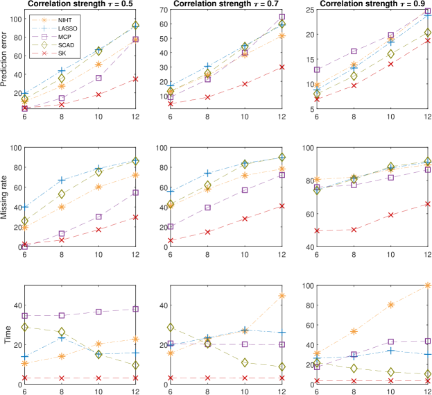
Figure 2: Regression: performance comparison in terms of prediction error, missing rate and computational time when varying the sparsity and the correlation strength of the model. In more details, $p=10\mbox{,}000,n=150,s=6,8,10,12$ and $\Sigma=[\tau 1_{i\neq j}]$ with $\tau=0.5,0.7,0.9$.

For classification, Table II and Figure 3 make a comparison between different methods with various correlation structures and problem dimensions, and similar conclusions can be drawn. It is important to note that the excellent statistical accuracy of slow kill is not accompanied by a sacrifice in computational time compared to other methods. In fact, as seen in Figure 3, slow kill offers substantial time savings especially when $n$ is large, while being very successful at selection and prediction.

TABLE II: Classification: performance comparison in terms of prediction error, missing rate and computational time with different correlation structures. In more details, $p=2\mbox{,}000,n=500,s=10$ and $\Sigma=[\tau^{|i-j|}]$ or $[\tau 1_{i\neq j}]$ with $\tau=0.9$

	Toeplitz structure				Equal correlation
	Error	Miss	Time		Error	Miss	Time
LASSO	8.0	24	10		5.1	95	49
ENET	8.0	25	31		4.7	95	135
MCP	6.9	23	15		5.0	93	20
SCAD	7.0	22	22		5.1	94	16
SK	2.2	2	4		3.9	78	4

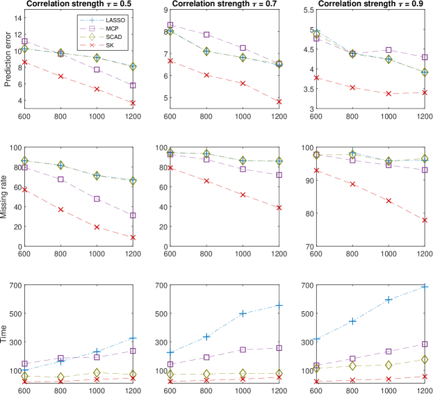
Figure 3: Classification: performance comparison in terms of prediction error, missing rate and computational time with different correlation structures and sample sizes. In more details, $p=10\mbox{,}000,n=600,800,1000,1200,s=15$ and $[\tau 1_{i\neq j}]$ with $\tau=0.5,0.7,0.9$.

Next, we present some experiments in which the signal strength is varied. Recall that in the regression setup, we set $\beta_{j}^{*}=1$ for $j\in\mathcal{J}(\beta^{*})$. For $n=100,p=5000,\sigma=1$, the minimax optimal rate is approximately $\sigma\sqrt{(\log p)/n}(\approx 0.292)$ (ignoring the constant factor for which a sharp value may be difficult to derive). We conducted additional experiments by setting $\beta_{j}^{*}=0.8,0.6,0.4,0.2$. The comparison results for different methods are demonstrated in Figure 4. As the signal strength was low (e.g., $\beta_{j}^{*}=0.2,0.4$), all methods performed poorly. For higher values, slow kill outperformed the other methods by a large margin.

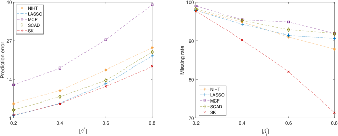
Figure 4: Comparison of prediction errors (left) and missing rates (right) of different methods under different signal strengths. The details of the regression setup are given in Section IV-A, and we set $p=5\mbox{,}000,n=100,s=10$, $\tau=0.8$, and $\beta_{j}^{*}=0.2,0.4,0.6,0.8$ for $j\in\mathcal{J}(\beta^{*})$.

We conducted another experiment to explore larger values of $\|\beta^{*}\|_{2}^{2}$. (As a reminder, in the previous setting where $s=10$ and $\beta_{j}^{*}=1$, $\forall j\in\mathcal{J}(\beta^{*})$, we had $\|\beta^{*}\|_{2}^{2}=10$.) We tested $\|\beta^{*}\|_{2}^{2}=50,100,150,200$ by scaling up each $\beta_{j}^{*}$ by a corresponding factor. The results of this experiment are shown in Figure 5. As $\|\beta^{*}\|_{2}^{2}$ increases, NIHT, MCP, and slow kill exhibit clear advantages, with the latter two showing similar prediction errors and missing rates.

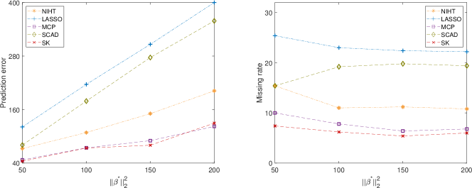
Figure 5: Comparison of prediction errors (left) and missing rates (right) of different methods for large signals. The details of the regression setup are given in Section IV-A, and we set $p=5\mbox{,}000,n=100,s=10$, $\tau=0.8$, and $\|\beta^{*}\|_{2}^{2}=50,100,150,200$ (by scaling up each $\beta_{j}^{*}$).

IV-B Handwritten digits classification

The Gisette dataset [33] was created to classify the highly confusing digits 4 and 9 for handwritten digit recognition. There are 5,000 predictors, including various pixel constructed features as well as some ‘probes’ with little predictive power. Because the exact number of relevant features is unknown, we assess the performance of different methods given the same model cardinality to make a fair comparison. We randomly split the 7,000 samples into a training subset with 3,000 samples and a test subset with 4,000 samples for 20 times to report the average misclassification error rate and total computational time.

Due to the relatively large size of the data, computational efficiency is a major concern. Many statistical packages were unable to deliver meaningful results in a reasonable amount of time. Here, we compare the glmnet [34], logitboost [35, 36], picasso with the MCP option [37], and slow kill with different numbers of selected features.

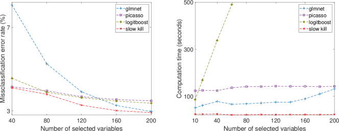
Figure 6: Gisette data. Left panel: mean misclassification error rate, right panel: total computational time, with different numbers of selected features. Picasso is too costly compared with the other methods and only part of its cost curve is shown.

According to Figure 6, logitboost and picasso achieved better misclassification error rates on the dataset than glmnet, but slow kill consistently performed the best. In terms of computational cost, glmnet and slow kill were extremely scalable; logitboost was quite expensive even for just $q=40$, and picasso suffered a similar issue when $q\geq 60$.

IV-C Breast cancer microarray data

The breast-cancer microarray dataset [38] from the Curated Microarray Database contains 35,981 gene expression levels of 143 tumor samples of patients with breast cancer and 146 paired adjacent normal breast tissue samples. The goal is to identify some differentially expressed genes to help the classification of normal and tumor tissues. We randomly split the dataset into a training subset (60%) and a test subset (40%) for 20 times and report the misclassification error rates and total computational time of different methods in Table III.

TABLE III: Breast cancer microarray data: misclassification error rate ($\times 100\%$) and total computational time (in seconds)

	$q=60$		$q=80$		$q=100$		$q=120$		$q=140$
	Error	Time	Error	Time	Error	Time	Error	Time	Error	Time
GLMNET	10.9	19	10.7	19	10.5	50	10.2	50	10.2	50
PICASSO	11.4	43	11.3	43	11.1	48	11.3	48	11.2	42
LogitBoost	11.2	500	11.2	680	10.9	860	10.6	1080	10.8	1220
SK	10.8	10	10.2	11	10.2	11	10.1	11	9.8	11

According to Tables III, logitboost has the highest computational complexity, and picasso shows the worst overall classification performance on this dataset. In contrast, glmnet and slow kill can achieve lower misclassification error rates, and the latter is much more cost-effective according to our experiments.

IV-D Sub-Nyquist spectrum sensing and learning

Sub-Nyquist sampling-based wideband spectrum sensing for millimeter wave is an important topic for next-generation wireless communication systems. With a multi-coset sampler [39], a multiple-measurement-vector model in signal processing can be formulated as $Y=XB^{*}+\mathcal{E}$, where the goal is to exploit the joint (row-wise) weak sparsity of $B^{*}$ to reconstruct the spectrum. Here, all the matrices are complex (e.g., $Y\in\mathbb{C}^{n\times m}$, $X\in\mathbb{C}^{n\times p}$), and the size of the predictor matrix $X$ is determined by the number of cosets and the number of channels; interested reader may refer to [40] for more detail. Nicely, with the Hermitian inner product $\langle A,B\rangle\triangleq\mbox{tr}\{A^{\mbox{\tiny H}}B\}$ in place of the real inner product, and the generalized Bregman function redefined as ${\mathbf{\Delta}}_{l}(B_{1},B_{2})=l(B_{1})-l(B_{2})-\langle\nabla l(B_{2}),B_{1}-B_{2}\rangle/2-\langle B_{1}-B_{2},\nabla l(B_{2})\rangle/2$, all of our theorems and algorithms can be extended to the complex group sparsity pursuit.

We compared our method with two popular methods, SOMP [41] and JB-HTP [42], on a benchmark time-domain dataset in [43]. Table IV shows the normalized mean square error $\|\hat{B}-B^{*}\|_{F}/\|B^{*}\|_{F}$ of each method as we vary $q$ (the number of selected channels). A demonstration of spectral recovery is plotted in Figure 7, where the predictive information criterion in Appendix A-H was used for model selection in slow kill.

TABLE IV: Spectrum reconstruction error in terms of normalized mean square error

	$q=3$	$q=4$	$q=5$	$q=6$	$q=7$	$q=8$
SOMP	0.83	0.93	0.82	0.91	0.92	0.94
JB-HTP	0.94	1.00	0.99	0.95	1.07	0.96
SK	0.74	0.65	0.53	0.38	0.42	0.50

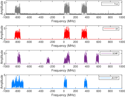
Figure 7: Spectrum sensing results by different methods.

V Summary

This paper proposed a new slow kill method for large-scale variable selection. It is a scalable optimization-based algorithm that uses three carefully designed and theoretically justified sequences of thresholds, shrinkage, and learning rates.

Intuitively, slow kill uses a novel backward quantile control with adaptive $\ell_{2}$ shrinkage and increasing learning rates to relax regularity conditions and overcome obstacles in backward elimination. This method is significantly different from boosting and many forward stagewise procedures in the existing literature. Our theoretical studies led to insights on how to design a progressive hybrid regularization to achieve the optimal error rate and fast convergence. The technique is applicable to a general loss that is not necessarily a negative log-likelihood function, and its ability to reduce the problem size throughout the iteration makes it attractive for big data.

Appendix A Proofs

The definition of a sub-Gaussian random variable or a sub-Gaussian random vector is standard in the literature.

Definition A.1.

We call $\xi$ a sub-Gaussian random variable if it has mean zero and the scale ($\psi_{2}$-norm) for $\xi$, defined as $\inf\{\sigma>0:\,\mathbb{E}[\exp(\xi^{2}/\sigma^{2})]\leq 2\}$, is finite. We call $\xi\in\mathbb{R}^{p}$ a sub-Gaussian random vector with scale bounded by $\sigma$ if all one-dimensional marginals $\langle\xi,\alpha\rangle$ are sub-Gaussian satisfying $\|\langle\xi,\alpha\rangle\|_{\psi_{2}}\leq\sigma\|\alpha\|_{2}$, $\mbox{for any}\ \alpha\in\mathbb{R}^{p}$. Similarly, a random matrix $\xi$ is called sub-Gaussian if $\operatorname{\mbox{vec}\,}(\xi)$ is sub-Gaussian.

A-A Theorem A.1 and Theorem 4

First, for the algorithm (5) defined in the setup of Section II, we have the following numerical properties.

Theorem A.1.

Given any $X,y$ and $\beta^{(0)}$, the sequence of iterates $\beta^{(t)}$ generated by (5) satisfies $f(\beta^{(t)})-f(\beta^{(t+1)})\geq{\rho}\|\beta^{(t+1)}-\beta^{(t)}\|_{2}^{2}/2-\|X(\beta^{(t+1)}-\beta^{(t)})\|_{2}^{2}/2,\ \forall t\geq 0$ and so when $\rho\geq\rho_{+}(2q)$, $f(\beta^{(t)})$ converges, and $\beta^{(t)}$ satisfies

$$\min_{0\leq t\leq T}\|\beta^{(t+1)}-\beta^{(t)}\|_{2}^{2}\leq\frac{1}{T+1}\frac{2f(\beta^{(0)})}{\rho-\rho_{+}(2q)}.$$

Moreover, as long as $\rho>\rho_{+}(2q)$ and $\eta_{0}>0$, $\beta^{(t)}$ has a unique limit point $\hat{\beta}$ that satisfies the “fixed-point” equation

$$\beta=\Theta^{\#}\{\beta-X^{T}(X\beta-y)/{\rho};q,\eta_{0}/\rho\},$$

and when $\|\hat{\beta}\|_{0}=q$, $\hat{\beta}$ is also a local minimizer of problem (3).

To prove the first conclusion in Theorem A.1, notice that in the regression setting,

$$g(\beta^{(t+1)},\beta^{(t)})-f(\beta^{(t+1)})=\rho\|\beta^{(t+1)}-\beta^{(t)}\|_{2}^{2}/2-\|X(\beta^{(t+1)}-\beta^{(t)})\|_{2}^{2}/2,$$

and thus

$$f(\beta^{(t)})-f(\beta^{(t+1)})\geq\frac{\rho}{2}\|\beta^{(t+1)}-\beta^{(t)}\|_{2}^{2}-\frac{1}{2}\|X(\beta^{(t+1)}-\beta^{(t)})\|_{2}^{2},\ \ \forall t\geq 0.$$

Taking the summation from $t=0$ to $t=T$ and using the fact that $\|X(\beta^{(t+1)}-\beta^{(t)})\|_{2}^{2}\leq\rho_{+}(2q)\|\beta^{(t+1)}-\beta^{(t)}\|_{2}^{2},$ we have

$$\frac{(\rho-\rho_{+}(2q))}{2}\sum_{t=0}^{T}\|\beta^{(t+1)}-\beta^{(t)}\|_{2}^{2}\leq f(\beta^{(0)})-f(\beta^{(T+1)}),$$

which leads to

$$\min_{0\leq t\leq T}\|\beta^{(t+1)}-\beta^{(t)}\|_{2}^{2}\leq\frac{2}{(T+1)(\rho-\rho_{+}(2q))}f(\beta^{(0)}).$$

Next, we consider the general problem and prove Theorem 4, which implies the second part of Theorem A.1. From $\inf_{\xi,y}l_{0}(\xi;y)>-\infty$, we assume without loss of generality that $l_{0}(\xi;y)\geq 0$. Recall $l_{0}(X\beta;y)$ is abbreviated as $l(\beta)$ and thus $\nabla l(\beta)=X^{T}\nabla l_{0}(X\beta)$ by the chain rule.

From the construction $g(\beta,\beta^{(t)})=f(\beta)+(\rho{\mathbf{D}}_{2}-{\mathbf{\Delta}}_{l_{0}})(\beta,\beta^{(t)})$, we get

$$(\rho{\mathbf{D}}_{2}-{\mathbf{\Delta}}_{l_{0}})(\beta^{(t+1)},\beta^{(t)})+f(\beta^{(t+1)})\leq g(\beta^{(t)},\beta^{(t)})=f(\beta^{(t)}).$$

When $\rho\geq\rho^{l}_{+}(q,q)$, $(\rho{\mathbf{D}}_{2}-{\mathbf{\Delta}}_{l_{0}})(\beta^{(t+1)},\beta^{(t)})\geq 0$, from which it follows that the sequence of $f(\beta^{(t)})$ is non-increasing and convergent. In fact, one just needs

$$f(\beta^{(t+1)})\leq g(\beta^{(t+1)},\beta^{(t)})$$ (A.1)

to enjoy the function value convergence, which can be used for line search.

In addition, we obtain

$$(\rho-\rho_{+}^{l}(q,q)){\mathbf{D}}_{2}(\beta^{(t+1)},\beta^{(t)})\leq f(\beta^{(t)})-f(\beta^{(t+1)}).$$

Finally, let us study the limit points of the sequence of iterates. We first notice that $\{\beta^{(t)}\}^{\infty}_{t=0}$ is uniformly bounded under $\eta_{0}>0$, since

$$\eta_{0}\|\beta^{(t)}\|_{2}^{2}/2\leq f(\beta^{(t)})\leq f(\beta^{(0)}).$$

From $\lim_{t\to\infty}\{f(\beta^{(t)})-f(\beta^{(t+1)})\}=0$, $\lim_{t\to\infty}(\rho{\mathbf{D}}_{2}-{\mathbf{\Delta}}_{l_{0}})(\beta^{(t+1)},\beta^{(t)})=0$, and because $\rho>\rho^{l}_{+}(q,q)$,

$$\lim_{t\to\infty}(\beta^{(t+1)}-\beta^{(t)})=0.$$

Let $\hat{\beta}$ be any limit point of $\beta^{(t)}$ satisfying $\hat{\beta}=\lim_{k\to\infty}\beta^{(j_{k})}$ for some sequence $j_{k}$. Then

$$0=\lim_{k\to\infty}(\beta^{(j_{k}+1)}-\beta^{(j_{k})}) =\lim_{k\to\infty}\Theta^{\#}\{\beta^{(j_{k})}-\nabla l(\beta^{(j_{k})})/\rho;q,\eta_{0}/\rho\}-\hat{\beta}$$

$$=\Theta^{\#}\{\hat{\beta}-\nabla l(\hat{\beta})/\rho;q,\eta_{0}/\rho\}-\hat{\beta},$$

where the second equality is due to the continuity of $\nabla l(\beta)$ and the $\Theta^{\#}$-uniqueness assumption.

Define ${\hat{\mathcal{J}}}=\{j:\hat{\beta}_{j}\neq 0\}$. Then we get

$$\hat{\beta}_{\hat{\mathcal{J}}}=\hat{\beta}_{\hat{\mathcal{J}}}/(1+\eta_{0}/\rho)-X_{\hat{\mathcal{J}}}^{T}\nabla l_{0}(X_{\hat{\mathcal{J}}}\hat{\beta}_{\hat{\mathcal{J}}};y)/(\rho+\eta_{0}),$$

or equivalently,

$$\eta_{0}\hat{\beta}_{\hat{\mathcal{J}}}+X_{\hat{\mathcal{J}}}^{T}\nabla l_{0}(X_{\hat{\mathcal{J}}}\hat{\beta}_{\hat{\mathcal{J}}};y)=0.$$

Therefore, given $\hat{\mathcal{J}}$, $\hat{\beta}_{\hat{\mathcal{J}}}$ is a stationary point of

$$\min_{\gamma}l_{0}(X_{\hat{\mathcal{J}}}\gamma;y)+\eta_{0}\|\gamma\|_{2}^{2}/2.$$ (A.2)

When $l_{0}(\cdot;y)$ is convex and $\eta_{0}>0$, (A.2) is strongly convex and thus $\hat{\beta}_{\hat{\mathcal{J}}}$ is the unique minimizer.

By Ostrowski’s convergence theorem, the set of limit points of $\beta^{(t)}$ must be connected. On the other hand, the set of all restricted optimal solutions $\{\hat{\beta}_{\hat{\mathcal{J}}}\}$ is finite, and so

$$\lim_{t\to\infty}\beta^{(t)}=\hat{\beta}.$$

Under $\|\hat{\mathcal{J}}\|_{0}=q$, it is easy to see that the neighborhood $\{\beta:\|\beta-\hat{\beta}\|_{\infty}<\epsilon,\;J(\beta)\leq q\}$ with $0<\epsilon<\min_{j\in\hat{\mathcal{J}}}\lvert\hat{\beta}_{j}\lvert$ is just $\{\beta:\mathcal{J}(\beta)=\hat{\mathcal{J}},|\beta_{j}-\hat{\beta}_{j}|<\epsilon,\forall j\in\hat{\mathcal{J}}\}$. The local optimality of $\hat{\beta}$ and support stability of $\beta^{(t)}$ thus follow.

A-B Proof of Theorem 1

We first introduce some lemmas that are helpful in proving the theorem. The first is a generalization of Lemma 9 in [44].

Lemma A.1.

Let $\mathcal{J}(B)$ denote the row support of matrix $B$ and define $J(B)=\|B\|_{2,0}=|\mathcal{J}(B)|$. Consider the following problem with $0\leq q\leq p,\eta\geq 0$:

$$\min_{B\in\mathbb{R}^{p\times m}}\frac{1}{2}\|Y-B\|_{F}^{2}+\frac{\eta}{2}\|B\|_{F}^{2}=l(B)\quad\mbox{subject to}\ \|B\|_{2,0}\leq q.$$

Then $\hat{B}=\vec{\Theta}^{\#}(Y;q,\eta)$ (recall $\vec{\Theta}^{\#}$ defined in Section I) gives a globally optimal solution, and for any $B$ satisfying $J(B)\leq s$, we have

$$l(B)-l(\hat{B})\geq(1-\mathcal{L}(\mathcal{J},\hat{\mathcal{J}}))(1+\eta)\frac{\|\hat{B}-B\|_{F}^{2}}{2}$$ (A.3)

where $\mathcal{J}=\mathcal{J}(B)$, $\hat{\mathcal{J}}=\mathcal{J}(\hat{B})$, and $\mathcal{L}(\mathcal{J},\hat{\mathcal{J}})=\sqrt{|\mathcal{J}\setminus\hat{\mathcal{J}}|/|\hat{\mathcal{J}}\setminus\mathcal{J}|}$. When $J(\hat{B})=q$ with $\vartheta(\equiv q/s)\geq 1$, $\mathcal{L}(\mathcal{J},\hat{\mathcal{J}})\leq\sqrt{|\mathcal{J}|/|\hat{\mathcal{J}}|}\leq 1/\sqrt{\vartheta}$. In the above statement, $0/0$ is understood as $1$.

Lemma A.2.

There exist universal constants $A,C,c>0$ such that for any $a>0$, the following event

$$\sup_{\beta_{1},\beta_{2}}\langle\epsilon,X(\beta_{1}-\beta_{2})\rangle-\frac{1}{2a}\|X(\beta_{1}-\beta_{2})\|_{2}^{2}-\frac{a}{2}A\sigma^{2}\{J(\beta_{1})\vee J(\beta_{2})\}\log\Big{\{}\frac{ep}{J(\beta_{1})\vee J(\beta_{2})}\Big{\}}\geq\frac{a}{2}\sigma^{2}t$$ (A.4)

occurs with probability at most $C\exp{(-ct)}p^{-{c}A}$, where $t\geq 0$.

First, by definition, it is easy to show that $\hat{\beta}$ satisfies

$$\hat{\beta}\in\operatorname*{argmin}_{\beta}g(\beta,\hat{\beta}),$$

where $g(\beta,\beta^{-})=\lVert y-X\beta^{-}\rVert_{2}^{2}/2+\langle X^{T}(X\beta^{-}-y),\beta-\beta^{-}\rangle+{\rho}\lVert\beta-\beta^{-}\rVert_{2}^{2}/2+\eta_{0}\|\beta\|_{2}^{2}/2$. By $g(\hat{\beta},\hat{\beta})\leq g(\beta^{*},\hat{\beta})$ and Lemma A.1,

$$\begin{split}\frac{1}{2}\|\beta^{*}-\hat{\beta}+\frac{1}{\rho}X^{T}(X\hat{\beta}-y)\|_{2}^{2}-\frac{1}{2}\|\frac{1}{\rho}X^{T}(X\hat{\beta}-y)\|_{2}^{2}+\frac{\eta_{0}}{2\rho}\|\beta^{*}\|_{2}^{2}-\frac{\eta_{0}}{2\rho}\|\hat{\beta}\|_{2}^{2}\\ \geq(1+\frac{\eta_{0}}{\rho})\frac{1-\mathcal{L}(\mathcal{J}^{*},\mathcal{\hat{J}})}{2}\|\hat{\beta}-\beta^{*}\|_{2}^{2},\end{split}$$

where $\mathcal{J}^{*}=\mathcal{J}(\beta^{*})$, $\mathcal{\hat{J}}=\mathcal{J}(\hat{\beta})$, and $\mathcal{L}(\mathcal{J}^{*},\mathcal{\hat{J}})\leq 1/\sqrt{\vartheta}$.

It follows from the model $y=X\beta^{*}+\epsilon$ that

$$\|X\hat{\beta}-X\beta^{*}\|_{2}^{2}+\frac{\eta_{0}}{2}\|\hat{\beta}\|_{2}^{2}\leq\frac{\rho-(\sqrt{\vartheta}-1)\eta_{0}}{2\sqrt{\vartheta}}\|\hat{\beta}-\beta^{*}\|_{2}^{2}+\frac{\eta_{0}}{2}\|\beta^{*}\|_{2}^{2}+\langle X\hat{\beta}-X\beta^{*},\epsilon\rangle,$$

which gives

$$\|X\hat{\beta}-X\beta^{*}\|_{2}^{2}+\frac{\eta_{0}}{2}\|\hat{\beta}-\beta^{*}\|_{2}^{2}$$

$$\leq \frac{\rho-(\sqrt{\vartheta}-1)\eta_{0}}{2\sqrt{\vartheta}}\|\hat{\beta}-\beta^{*}\|_{2}^{2}+\eta_{0}\langle\hat{\beta}-\beta^{*},-\beta^{*}\rangle+\langle X\hat{\beta}-X\beta^{*},\epsilon\rangle$$

$$\leq \frac{\rho-(\sqrt{\vartheta}-1)\eta_{0}}{2\sqrt{\vartheta}}\|\hat{\beta}-\beta^{*}\|_{2}^{2}+\frac{b\eta_{0}}{2}\|\hat{\beta}-\beta^{*}\|_{2}^{2}+\frac{\eta_{0}}{2b}\|\beta^{*}\|_{2}^{2}+\langle X\hat{\beta}-X\beta^{*},\epsilon\rangle$$ (A.5)

for any $b>0$. Applying Lemma A.2 with $t=0$, we can show that for any $a>0$, the following event

$$\langle X\hat{\beta}-X\beta^{*},\epsilon\rangle\leq\frac{1}{2a}\|X\hat{\beta}-X\beta^{*}\|_{2}^{2}+\frac{a}{2}A\sigma^{2}\vartheta s\log{\frac{ep}{\vartheta s}}$$ (A.6)

occurs with probability at least $1-Cp^{-c}$, where $A,C,c>0$ are some universal constants.

Combining (A.5), (A.6) and the regularity condition (7) yields

$$\frac{\eta_{0}(\varepsilon-b)}{2}\|\hat{\beta}-\beta^{*}\|_{2}^{2}+\Big{(}\frac{\delta}{2}-\frac{1}{2a}\Big{)}\|X\hat{\beta}-X\beta^{*}\|_{2}^{2}\leq\frac{\eta_{0}}{2b}\|\beta^{*}\|_{2}^{2}+\frac{a}{2}A\sigma^{2}\vartheta s\log{\frac{ep}{\vartheta s}}$$

with probability at least $1-Cp^{-c}$. By choosing $a=2/\delta$ and $b=\varepsilon/2$, we have the bound for the prediction error as

$$\|X\hat{\beta}-X\beta^{*}\|_{2}^{2}+\frac{\eta_{0}\varepsilon}{\delta}\|\hat{\beta}-\beta^{*}\|_{2}^{2} \leq\frac{4\eta_{0}}{\delta\varepsilon}\|\beta^{*}\|_{2}^{2}+\frac{4}{\delta^{2}}A\sigma^{2}\vartheta s\log{\frac{ep}{\vartheta s}}$$

$$\lesssim\frac{\eta_{0}}{\delta\varepsilon}\|\beta^{*}\|_{2}^{2}+\frac{1}{\delta^{2}}\sigma^{2}\vartheta s\log{\frac{ep}{\vartheta s}},$$

which holds with probability at least $1-Cp^{-c}$.

Proof of Lemma A.1 In this proof, given a matrix $B\in\mathbb{R}^{p\times m}$ and an index set $\mathcal{I}\subset[p]$, we use $B_{\mathcal{I}}$ to denote the submatrix of $B$ by extracting its rows indexed by $\mathcal{I}$. Let $\mathcal{J}_{1}=\mathcal{J}\cap\hat{\mathcal{J}}$, $\mathcal{J}_{2}=\hat{\mathcal{J}}\setminus\mathcal{J}$ and $\mathcal{J}_{3}=\mathcal{J}\setminus\hat{\mathcal{J}}$. Then $\mathcal{J}=\mathcal{J}_{1}\cup\mathcal{J}_{3}$ and $\hat{\mathcal{J}}=\mathcal{J}_{1}\cup\mathcal{J}_{2}$.

It can be easily shown that $\hat{B}_{\mathcal{J}_{1}}=Y_{{\mathcal{J}}_{1}}/(1+\eta)$ and $\hat{B}_{\mathcal{J}_{2}}=Y_{{\mathcal{J}}_{2}}/(1+\eta)$. By writing $B_{\mathcal{J}_{1}}=Y_{{\mathcal{J}}_{1}}/(1+\eta)+\Delta_{{\mathcal{J}}_{1}}$ and $B_{\mathcal{J}_{3}}=Y_{{\mathcal{J}}_{3}}/(1+\eta)+\Delta_{{\mathcal{J}}_{3}}$, we have

$$l(B)-l(\hat{B}) =\frac{1+\eta}{2}\|\Delta_{{\mathcal{J}}_{1}}\|_{F}^{2}+\frac{1}{2(1+\eta)}\|Y_{{\mathcal{J}}_{2}}\|_{F}^{2}+\frac{1+\eta}{2}\|\Delta_{{\mathcal{J}}_{3}}\|_{F}^{2}-\frac{1}{2(1+\eta)}\|Y_{{\mathcal{J}}_{3}}\|_{F}^{2},$$

$$\frac{1+\eta}{2}\|\hat{B}-B\|_{F}^{2} =\frac{1+\eta}{2}\|\Delta_{{\mathcal{J}}_{1}}\|_{F}^{2}+\frac{1}{2(1+\eta)}\|Y_{{\mathcal{J}}_{2}}\|_{F}^{2}+\frac{1+\eta}{2}\|\frac{1}{1+\eta}Y_{{\mathcal{J}}_{3}}+\Delta_{{\mathcal{J}}_{3}}\|_{F}^{2}.$$

Let $K\leq 1$ satisfy

$$l(B)-l(\hat{B})\geq\frac{K}{2}(1+\eta)\|\hat{B}-B\|_{F}^{2},$$

which is implied by

$$\begin{split}&\frac{1}{2(1+\eta)}\|Y_{{\mathcal{J}}_{2}}\|_{F}^{2}+\frac{1+\eta}{2}\|\Delta_{{\mathcal{J}}_{3}}\|_{F}^{2}-\frac{1}{2(1+\eta)}\|Y_{{\mathcal{J}}_{3}}\|_{F}^{2}\\ \geq\ &\frac{K}{2(1+\eta)}\|Y_{{\mathcal{J}}_{2}}\|_{F}^{2}+\frac{K(1+\eta)}{2}\|\frac{1}{1+\eta}Y_{{\mathcal{J}}_{3}}+\Delta_{{\mathcal{J}}_{3}}\|_{F}^{2}.\end{split}$$ (A.7)

(A.7) is equivalent to

$$\begin{split}&(1-K)\|Y_{{\mathcal{J}}_{2}}\|_{F}^{2}+(1+\eta)^{2}\|\Delta_{{\mathcal{J}}_{3}}\|_{F}^{2}\geq(1+\eta)^{2}K\|\frac{1}{1+\eta}Y_{{\mathcal{J}}_{3}}+\Delta_{{\mathcal{J}}_{3}}\|_{F}^{2}+\|Y_{{\mathcal{J}}_{3}}\|_{F}^{2}.\end{split}$$ (A.8)

By construction, $\|y_{i}\|_{2}\geq\|y_{j}\|_{2}$ for any $i\in{\mathcal{J}}_{2}$ and $j\in{\mathcal{J}}_{3}$. Thus $\|Y_{{\mathcal{J}}_{2}}\|_{F}^{2}\geq J_{2}\|Y_{{\mathcal{J}}_{3}}\|_{F}^{2}/J_{3}$, from which it follows that (A.8) is implied by

$$\{(1-K)({J_{2}}/{J_{3}})-(1+K)\}\|Y_{{\mathcal{J}}_{3}}\|_{F}^{2}+(1-K)(1+\eta)^{2}\|\Delta_{{\mathcal{J}}_{3}}\|_{F}^{2}\geq 2K(1+\eta)\langle Y_{{\mathcal{J}}_{3}},\Delta_{{\mathcal{J}}_{3}}\rangle.$$

Therefore, restricting $K$ to $(1+K)/(1-K)\leq{J_{2}}/{J_{3}}$ or $K\leq(J_{2}-J_{3})/(J_{2}+J_{3})\leq 1$, the largest possible $K$ should satisfy

$$\{(1-K)({J_{2}}/{J_{3}})-(1+K)\}\cdot({1-K})=|K|^{2}$$

or $(1-K)^{2}=J_{3}/J_{2}$, or $K=1-\sqrt{J_{3}/J_{2}}(\leq(J_{2}-J_{3})/(J_{2}+J_{3}))$. This gives

$$\mathcal{L}=1-K=({{J_{3}}/{J_{2}}})^{1/2}.$$

Note that when $\mathcal{J}_{2}=\emptyset$, $K$ can take $-\infty$ for $\mathcal{J}_{3}\neq\emptyset$ and $0$ for $\mathcal{J}_{3}=\emptyset$ to ensure (A.8).

Now assume $J(\hat{B})=q$ with $\vartheta\geq 1$. If $\mathcal{J}_{2}\neq\emptyset$, $\mathcal{L}\leq\sqrt{({J_{3}+J_{1}})/({J_{2}+J_{1}})}=\sqrt{{J}/{\hat{J}}}\leq 1/\sqrt{\vartheta}$. Otherwise, we must have $\mathcal{J}_{3}=\emptyset$, $\mathcal{J}=\hat{\mathcal{J}}$ and $\vartheta=1$. The proof is complete.

The lemma can be used in the analysis of $\ell_{0}$-constrained (elementwise) sparsity pursuit, as well as group variable selection (cf. Section IV-D).

Proof of Lemma A.2 Given a matrix $A$, denote by $\mathcal{P}_{A}$ the orthogonal projection onto its range, and $\mathcal{P}_{A}^{\perp}$ its orthogonal complement. In the proof, $\mathcal{P}_{\mathcal{J}}$ is used as a short notation for $\mathcal{P}_{X_{\mathcal{J}}}$ in the proof for any $J\subset[p]$. Let $\mathcal{J}_{1}=\mathcal{J}(\beta_{1}),\mathcal{J}_{2}=\mathcal{J}(\beta_{2}),J_{1}=|\mathcal{J}_{1}|,J_{2}=|\mathcal{J}_{2}|$.

First, note that the term $\{J(\beta_{1})\vee J(\beta_{2})\}\log[ep/\{J(\beta_{1})\vee J(\beta_{2})\}]$ is used in (A.4), instead of $J(\beta_{1}-\beta_{2})\log\{ep/J(\beta_{1}\allowbreak-\beta_{2})\}$, and although $J(\beta_{1}-\beta_{2})\leq J(\beta_{1})+J(\beta_{2})$, $J(\beta_{1})+J(\beta_{2})$ can be larger than $p$. To tackle the issue, we employ a decomposition trick

$$X\beta_{1}-X\beta_{2} =\mathcal{P}_{\mathcal{J}_{1}}X(\beta_{1}-\beta_{2})+\mathcal{P}_{\mathcal{J}_{1}}^{\perp}X(\beta_{1}-\beta_{2})$$

$$=\mathcal{P}_{\mathcal{J}_{1}}X(\beta_{1}-\beta_{2})+\mathcal{P}_{\mathcal{J}_{1}}^{\perp}\mathcal{P}_{\mathcal{J}_{2}}X(\beta_{1}-\beta_{2}).$$

Let $\Delta=\beta_{1}-\beta_{2}$. Then

$$\langle\epsilon,X\Delta\rangle=\langle\epsilon,P_{\mathcal{J}_{1}}X\Delta\rangle+\langle\epsilon,\mathcal{P}_{\mathcal{J}_{1}}^{\perp}\mathcal{P}_{\mathcal{J}_{2}}X\Delta\rangle.$$ (A.9)

Let us bound the first term on the right-hand side of (A.9). Define $P_{o}(J)=\sigma^{2}J\log(ep/J)$ for $0\leq J\leq p$, which is an increasing function, and $\Gamma_{J}=\{\alpha\in\mathbb{R}^{p}:\|\alpha\|_{2}\leq 1,\alpha\in\mathcal{P}_{\mathcal{J}}\ \mbox{for some}\ \mathcal{J}\subset[p],|\mathcal{J}|\leq J\}$. Then for any $a,b>0$

$$\langle\epsilon,\mathcal{P}_{\mathcal{J}_{1}}X\Delta\rangle-\frac{1}{a}\|\mathcal{P}_{\mathcal{J}_{1}}X\Delta\|_{2}^{2}-bLP_{o}(J_{1})$$

$$\leq\, \|\mathcal{P}_{\mathcal{J}_{1}}X\Delta\|_{2}\langle\epsilon,\frac{\mathcal{P}_{\mathcal{J}_{1}}X\Delta}{\|\mathcal{P}_{\mathcal{J}_{1}}X\Delta\|_{2}}\rangle-2\|\mathcal{P}_{\mathcal{J}_{1}}X\Delta\|_{2}\sqrt{\frac{b}{a}LP_{o}({J_{1}})}$$

$$\leq\, \frac{1}{a}\|\mathcal{P}_{\mathcal{J}_{1}}X\Delta\|^{2}_{2}+\frac{a}{4}\sup_{J_{1}\leq p}\sup_{\Delta\in\Gamma_{J_{1}}}\big{\{}\langle\epsilon,\Delta\rangle-2\sqrt{({b}/{a})LP_{o}(J_{1})}\big{\}}_{+}^{2}$$

$$\equiv\, \frac{1}{a}\|\mathcal{P}_{\mathcal{J}_{1}}X\Delta\|^{2}_{2}+\frac{a}{4}\sup_{J_{1}\leq p}R_{J_{1}}^{2},$$

where $R_{J_{1}}:=\sup_{\Delta\in\Gamma_{J_{1}}}\big{\{}\langle\epsilon,\Delta\rangle-2\sqrt{({b}/{a})LP_{o}(J_{1})}\big{\}}_{+}$ with $L$ a sufficiently large constant. When $J_{1}=0$, $R_{J_{1}}=0$. When $J_{1}\geq 1$, for any $t\geq 0$, if $4b/a$ is a constant greater than $1$, we have

$$\begin{split}&\mathbb{P}(\sup_{1\leq J_{1}\leq p}R_{J_{1}}\geq t\sigma)\\ \leq\,&\sum_{J_{1}=1}^{p}\mathbb{P}\bigg{(}\sup_{\Delta\in\Gamma_{J_{1}}}\langle\epsilon,\Delta\rangle-\sqrt{LP_{o}(J_{1})}\geq t\sigma+2\sqrt{\frac{b}{a}LP_{o}(J_{1})}-\sqrt{LP_{o}(J_{1})}\bigg{)}\\ \leq\,&C\exp(-ct^{2})\sum_{J_{1}=1}^{p}\exp[-c(2\sqrt{b/a}-1)^{2}LP_{o}(J_{1})/\sigma^{2}]\\ \leq\,&C\exp(-ct^{2})\exp(-cL\log p)\sum_{J_{1}=1}^{p}\exp(-cLJ_{1})\\ \leq\,&C\exp(-ct^{2})p^{-cL}.\end{split}$$ (A.10)

The second inequality is due to Lemma 6 of [21], and we used $J\log(ep/J)\geq J+\log p$ for any $J\in[p]$ in the third inequality. Therefore, for any $a,b>0,$ $4b>a$ and $t\geq 0$, we have

$$\,\mathbb{P}\Big{\{}\langle\epsilon,\mathcal{P}_{\mathcal{J}_{1}}X\Delta\rangle-\frac{2}{a}\|\mathcal{P}_{\mathcal{J}_{1}}X\Delta\|_{2}^{2}-bLP_{o}(J_{1})\geq\frac{a}{4}t\sigma^{2}\Big{\}}\leq C\exp(-ct)p^{-Lc}.$$ (A.11)

Similarly, for the second term in (A.9), we can use Lemma 7 of [13] to prove that for any $t\geq 0$,

$$\,\mathbb{P}\Big{[}\langle\epsilon,\mathcal{P}_{\mathcal{J}_{1}}^{\perp}\mathcal{P}_{\mathcal{J}_{2}}X\Delta\rangle-\frac{2}{a}\|\mathcal{P}_{\mathcal{J}_{1}}^{\perp}\mathcal{P}_{\mathcal{J}_{2}}X\Delta\|_{2}^{2}-bL\{P_{o}(J_{1})+P_{o}(J_{2})\}\geq\frac{a}{4}t\sigma^{2}\Big{]}\leq C\exp(-ct)p^{-Lc}.$$ (A.12)

Combining (A.11), (A.12) and using the fact that $\|\mathcal{P}_{\mathcal{J}_{1}}X\Delta\|_{2}^{2}+\|\mathcal{P}_{\mathcal{J}_{1}}^{\perp}\mathcal{\mathcal{missing}}{P}_{\mathcal{J}_{2}}X\Delta\|_{2}^{2}=\|X\Delta\|_{2}^{2},$ we get for any $a,b>0,$ $4b>a$ and $t\geq 0$,

$$\,\mathbb{P}\Big{[}\langle\epsilon,X\Delta\rangle-\frac{4}{a}\|X\Delta\|_{2}^{2}-3bL\{P_{o}(J_{1})\vee P_{o}(J_{2})\}\geq\frac{a}{2}t\sigma^{2}\Big{]}\leq C\exp(-ct)p^{-Lc}.$$ (A.13)

Finally, using the increasing property of $P_{o}(J)$ for $J\in[0,p]$, we have $P_{o}(J_{1})\vee P_{o}(J_{2})\leq(J_{1}\vee J_{2})\log\{ep/(J_{1}\vee J_{2})\}$. A reparameterization of (A.13) gives the conclusion.

A-C Proof of Theorem 2

From the proof of Theorem 1, we get with probability $1-Cp^{-c}$,

$$\|X\hat{\beta}-X\beta^{*}\|_{2}^{2}+\frac{\eta_{0}(1-b)}{2}\|\hat{\beta}-\beta^{*}\|_{2}^{2}\leq\, \frac{\rho-(\sqrt{\vartheta}-1)\eta_{0}}{2\sqrt{\vartheta}}\|\hat{\beta}-\beta^{*}\|_{2}^{2}+\frac{\eta_{0}}{2b}\|\beta^{*}\|_{2}^{2}+$$

$$\frac{1}{2a}\|X\hat{\beta}-X\beta^{*}\|_{2}^{2}+\frac{a}{2}A\sigma^{2}\vartheta s\log{\frac{ep}{\vartheta s}},$$

which gives

$$\|X\hat{\beta}-X\beta^{*}\|_{2}^{2}-\frac{\eta_{0}b}{2}\|\hat{\beta}-\beta^{*}\|_{2}^{2}\leq\, \frac{\rho-(2\sqrt{\vartheta}-1)\eta_{0}}{2\sqrt{\vartheta}}\|\hat{\beta}-\beta^{*}\|_{2}^{2}+\frac{\eta_{0}}{2b}\|\beta^{*}\|_{2}^{2}+$$

$$\frac{\rho_{+}((1+\vartheta)s)}{2a}\|\hat{\beta}-\beta^{*}\|_{2}^{2}+\frac{a}{2}A\sigma^{2}\vartheta s\log{\frac{ep}{\vartheta s}}.$$

Under the regularity condition (9), choosing $a=2/\delta$ and $b=\delta\rho_{+}((1+\vartheta)s)/(4\eta_{0})$ give (10). (The result applies to $\eta_{0}=0$ as well.)

To show the second result, note that from Theorem 1, the fixed-point solution $\hat{\beta}$ must satisfy $\hat{\beta}=\Theta^{\#}\{\hat{\beta}-X^{T}\nabla l_{0}(X\hat{\beta};y)/\rho;q,\eta_{0}/\rho\}$, which means

$$\Big{\|}\hat{\beta}(1+\eta_{0}/\rho)-\hat{\beta}+\frac{1}{\rho}X^{T}\nabla l_{0}(X\hat{\beta})\Big{\|}_{\infty}\leq(1+\eta_{0}/\rho)\min_{j\in\hat{\mathcal{J}}}|\hat{\beta}_{j}|$$

$$\implies \Big{\|}\eta_{0}\hat{\beta}+X^{T}(\nabla l_{0}(X\hat{\beta})-\nabla l_{0}(X\beta^{*}))-X^{T}\epsilon\Big{\|}_{\infty}\leq(\rho+\eta_{0})\min_{j\in\hat{\mathcal{J}}}|\hat{\beta}_{j}|$$

$$\implies \left\|X^{T}(\nabla l_{0}(X\hat{\beta})-\nabla l_{0}(X\beta^{*}))+\eta_{0}(\hat{\beta}-\beta^{*})\right\|_{\infty}\leq\|X^{T}\epsilon\|_{\infty}+\eta_{0}\|\beta^{*}\|_{\infty}+(\rho+\eta_{0})\min_{j\in\hat{\mathcal{J}}}|\hat{\beta}_{j}|.$$

Next, we introduce a lemma.

Lemma A.3.

Let $\tilde{\beta},\beta\in\mathbb{R}^{p}$ satisfying $\|\tilde{\beta}\|_{0}=q>s\geq\|\beta\|_{0}$, and for short, denote $\mathcal{J}(\tilde{\beta})$ and $\mathcal{J}(\tilde{\beta})$ by $\tilde{\mathcal{J}}$ and $\mathcal{J}$, respectively. Then

$$\min_{j\in\tilde{\mathcal{J}}}|\tilde{\beta}_{j}|\leq\min_{j\in\tilde{\mathcal{J}}\setminus\mathcal{J}}|\tilde{\beta}_{j}|\leq\frac{\|(\tilde{\beta}-\beta)_{\tilde{\mathcal{J}}\setminus\mathcal{J}}\|_{2}}{\sqrt{|\tilde{\mathcal{J}}\setminus\mathcal{J}|}}\leq\frac{\|(\tilde{\beta}-\beta)_{\tilde{\mathcal{J}}\setminus\mathcal{J}}\|_{2}}{\sqrt{q-s}}\leq\frac{\|\tilde{\beta}-\beta\|_{2}}{\sqrt{q-s}}$$ (A.14)

$$\min_{j\in\tilde{\mathcal{J}}}|\tilde{\beta}_{j}|\leq\max_{j\in\tilde{\mathcal{J}}\setminus\mathcal{J}}|\tilde{\beta}_{j}|=\|(\tilde{\beta}-\beta)_{\tilde{\mathcal{J}}\setminus\mathcal{J}}\|_{\infty}\leq\|\tilde{\beta}-\beta\|_{\infty.}$$ (A.15)

The proof is simple and omitted. Now, combining the regularity condition (11) and (A.14) or (A.15) gives the desired result.

A-D Proof of Theorem 3

By definition, we have

$$\rho_{+}(2q)=\sup_{I\in[p]:|I|=2q}\lambda_{\max}(X_{I}^{T}X_{I}),$$

and under $q+s\leq n,$

$$\rho_{-}(q+s)=\inf_{I\in[p]:|I|=q+s}\lambda_{\min}(X_{I}^{T}X_{I}).$$

By Theorem of 6.1 of [23], we have

$$\mathbb{P}\left\{\sqrt{\frac{\lambda_{\max}(X_{I}^{T}X_{I})}{n}}\geq(1+c_{0})\sqrt{\lambda_{\max}(\Sigma_{I})}+\sqrt{\frac{\operatorname{tr}(\Sigma_{I})}{n}}\right\}\leq\exp(-nc_{0}^{2}/2),\ \ \forall I:|I|=2q$$

and

$$\mathbb{P}\left\{\sqrt{\frac{\lambda_{\min}(X_{I}^{T}X_{I})}{n}}\leq(1-c_{0})\sqrt{\lambda_{\min}(\Sigma_{I})}-\sqrt{\frac{\operatorname{tr}(\Sigma_{I})}{n}}\right\}\leq\exp(-nc_{0}^{2}/2),\ \ \forall I:|I|=q+s$$

for all $c_{0}>0$. Applying the union bound gives

$$\mathbb{P}\left\{\sqrt{\frac{\rho_{+}(2q)}{n}}\geq(1+c_{0})\sqrt{\lambda^{(2q)}_{\max}}+\sqrt{\frac{2q}{n}}\right\}\leq\binom{p}{2q}\exp(-nc_{0}^{2}/2).$$ (A.16)

Let $nc^{2}=nc_{0}^{2}-\log\binom{p}{2q}.$ Then using $\log\binom{p}{2q}\leq 2q\log{(ep/q)}$, $c_{0}\leq c+\sqrt{2q\log(ep/q)/n}$. Therefore for any $c>0$,

$$\,\mathbb{P}\left\{\sqrt{\frac{\rho_{+}(2q)}{n}}\geq(1+c)\sqrt{\lambda^{(2q)}_{\max}}+\sqrt{\frac{2q\log(ep/q)}{n}}\sqrt{\lambda^{(2q)}_{\max}}+\sqrt{\frac{2q}{n}}\right\}\leq\exp(-nc^{2}/2).$$ (A.17)

Similarly,

$$\,\mathbb{P}\left\{\sqrt{\frac{\rho_{-}(q+s)}{n}}\leq(1-c)\sqrt{\lambda^{(q+s)}_{\min}}-\sqrt{\frac{(q+s)\log(ep/q)}{n}}\sqrt{\lambda^{(q+s)}_{\min}}-\sqrt{\frac{q+s}{n}}\right\}\leq\exp(-nc^{2}/2).$$

Let $c\in(0,1)$ and assume $n\geq\{2(q+s)/(1-c)^{2}\}\{1/\lambda^{(q+s)}_{\min}+\log(ep/q)\}.$ Then

$$\frac{\rho_{+}(2q)}{\rho_{-}(q+s)}\leq\left\{\frac{(1+c)\sqrt{\lambda^{(2q)}_{\max}}+\sqrt{\{2\lambda^{(2q)}_{\max}q\log(ep/q)\}/n}+\sqrt{2q/n}}{(1-c)\sqrt{\lambda^{(q+s)}_{\min}}-\sqrt{\{\lambda^{(q+s)}_{\min}(q+s)\log(ep/q)\}/n}-\sqrt{(q+s)/n}}\right\}^{2}$$

holds with probability at least $1-2\exp(-nc^{2}/2)$.

A-E Proof of Theorem 5

Let $E:=\sigma^{2}P_{o}(q)+\sigma^{2}$. Similar to the proof of Theorem 1, from the construction of $g$ and Lemma A.1, we have

$$\rho(1-1/\sqrt{\vartheta})(1+\eta_{0}/\rho){\mathbf{D}}_{2}(\beta^{*},\hat{\beta})+g(\hat{\beta},\hat{\beta})\leq g(\beta^{*},\hat{\beta}),$$

and thus

$$2\bar{\mathbf{\Delta}}_{l_{0}}(X\hat{\beta},X\beta^{*})+\frac{\eta_{0}}{2}\|\hat{\beta}\|_{2}^{2}\leq\frac{\rho-(\sqrt{\vartheta}-1)\eta_{0}}{\sqrt{\vartheta}}{\mathbf{D}}_{2}(\hat{\beta},\beta^{*})+\frac{\eta_{0}}{2}\|{\beta}^{*}\|_{2}^{2}+\langle\epsilon,X\hat{\beta}-X\beta^{*}\rangle.$$ (A.18)

Applying Lemma A.2 gives

$$\begin{split}\langle\epsilon,X\hat{\beta}-X\beta^{*}\rangle\leq\delta{\mathbf{D}}_{2}(X\hat{\beta},X\beta^{*})+\frac{1}{\delta}A\sigma^{2}P_{o}(q)+R\end{split}$$ (A.19)

for any $\delta>0$, where $R:=\sup_{\beta_{1},\beta_{2}}\{\langle\epsilon,X\beta_{1}-X\beta_{2}\rangle-\delta{\mathbf{D}}_{2}(X\beta_{1},X\beta_{2})-A\sigma^{2}P_{o}(q)/\delta\}_{+}$ and

$$\,\mathbb{P}(\delta R>\sigma^{2}t)\leq C\exp(-ct)p^{-cA},$$

where $A,C,c>0$ are some constants. Therefore,

$$\,\mathbb{E}\langle\epsilon,X\hat{\beta}-X\beta^{*}\rangle\leq\,\mathbb{E}\{\delta{\mathbf{D}}_{2}(X\hat{\beta},X\beta^{*})\}+\frac{C}{\delta}(\sigma^{2}P_{o}(q)+\sigma^{2}).$$ (A.20)

Combining (A.18) and (A.20) gives

$$\begin{split}&\,\mathbb{E}\{(2\bar{{\mathbf{\Delta}}}_{l_{0}}-\delta{\mathbf{D}}_{2})(X\hat{\beta},X\beta^{*})+\eta_{0}{\mathbf{D}}_{2}(\hat{\beta},\beta^{*})\}\\ \leq&\,\mathbb{E}\Big{\{}\frac{\rho-(\sqrt{\vartheta}-1)\eta_{0}}{\sqrt{\vartheta}}\ {\mathbf{D}}_{2}(\hat{\beta},\beta^{*})+\eta_{0}\langle-\beta^{*},\hat{\beta}-\beta^{*}\rangle\Big{\}}+\frac{C}{\delta}E,\end{split}$$ (A.21)

and so

$$\,\mathbb{E}\Big{[}(2\bar{{\mathbf{\Delta}}}_{l_{0}}-\delta{\mathbf{D}}_{2})(X\hat{\beta},X\beta^{*})-\frac{\rho-\{(2-\varepsilon)\sqrt{\vartheta}-1\}\eta_{0}}{\sqrt{\vartheta}}\ {\mathbf{D}}_{2}(\hat{\beta},\beta^{*})\Big{]}\\ \leq\frac{C}{\delta}E+\frac{\eta_{0}}{2\varepsilon}\|\beta^{*}\|_{2}^{2}$$ (A.22)

for any $\varepsilon,\delta>0$.

Next, from $l_{0}(X\hat{\beta})+\eta_{0}\|\hat{\beta}\|_{2}^{2}/2\leq l_{0}(X\beta^{(0)})+\eta_{0}\|{\beta}^{(0)}\|_{2}^{2}/2$, we have

$$\begin{split}&{\mathbf{\Delta}}_{l_{0}}(X\hat{\beta},X\beta^{*})+\eta_{0}{\mathbf{D}}_{2}(\hat{\beta},\beta^{*})\\ \leq&\,{\mathbf{\Delta}}_{l_{0}}(X\beta^{(0)},X\beta^{*})+\eta_{0}{\mathbf{D}}_{2}(\beta^{(0)},\beta^{*})+\eta_{0}\langle-\beta^{*},\hat{\beta}-\beta^{*}\rangle-\eta_{0}\langle-\beta^{*},\beta^{(0)}-\beta^{*}\rangle\\ &+\langle\epsilon,X\hat{\beta}-X\beta^{*}\rangle-\langle\epsilon,X{\beta}^{(0)}-X\beta^{*}\rangle.\end{split}$$ (A.23)

Therefore, for any $\delta^{\prime},\delta^{\prime\prime},\varepsilon^{\prime}>0$

$$\,\mathbb{E}\{({{\mathbf{\Delta}}}_{l_{0}}-\delta^{\prime}{\mathbf{D}}_{2})(X\hat{\beta},X\beta^{*})+\eta_{0}{\mathbf{D}}_{2}(\hat{\beta},\beta^{*})\}$$

$$\leq \,\mathbb{E}\big{\{}({\mathbf{\Delta}}_{l_{0}}+\delta^{\prime\prime}{\mathbf{D}}_{2})(X\beta^{(0)},X\beta^{*})+\eta_{0}{\mathbf{D}}_{2}(\beta^{(0)},\beta^{*})+\frac{\eta_{0}}{2\varepsilon}\|\beta^{*}\|_{2}^{2}+\eta_{0}\varepsilon{\mathbf{D}}_{2}(\hat{\beta},\beta^{*})$$

$$+\frac{\eta_{0}}{2\varepsilon^{\prime}}\|\beta^{*}\|_{2}^{2}+\eta_{0}\varepsilon^{\prime}{\mathbf{D}}_{2}(\beta^{(0)},\beta^{*})\big{\}}+CE\big{(}\frac{1}{\delta^{\prime}}+\frac{1}{\delta^{\prime\prime}}\big{)}.$$

By the assumption of the starting point $\,\mathbb{E}\{{\mathbf{D}}_{2}(\beta^{(0)},\beta^{*})\}\leq CME/n,$ we have

$$\,\mathbb{E}\{{\mathbf{D}}_{2}(X\beta^{(0)},X\beta^{*})\}\leq C\rho_{+}(q+s)ME/n,\,\mathbb{E}\{{\mathbf{\Delta}}_{l_{0}}(X\beta^{(0)},X\beta^{*})\}\leq C\rho^{l}_{+}(q,s)ME/n.$$

Taking $1/\delta^{\prime\prime}=\sqrt{\rho_{+}(q+s)M/n}$, we obtain

$$\,\mathbb{E}\{({{\mathbf{\Delta}}}_{l_{0}}-\delta^{\prime}{\mathbf{D}}_{2})(X\hat{\beta},X\beta^{*})+\eta_{0}(1-\varepsilon){\mathbf{D}}_{2}(\hat{\beta},\beta^{*})\}$$

$$\leq \,CE\big{(}\frac{1}{\delta^{\prime}}+\sqrt{\frac{\rho_{+}(q+s)M}{n}}+\frac{\rho_{+}^{l}(q,s)}{n}M+\frac{\eta_{0}(1+\varepsilon^{\prime})}{n}M\big{)}+\eta_{0}\big{(}\frac{1}{\varepsilon}+\frac{1}{\varepsilon^{\prime}}\big{)}\frac{\|\beta^{*}\|_{2}^{2}}{2}.$$

Let $Q_{0}:=\sqrt{\rho_{+}(q+s)M/n}+\rho_{+}^{l}(q,s)M/n+\eta_{0}(1+\varepsilon^{\prime})M/n$. Then

$$CE\big{(}\frac{1}{\delta^{\prime}}+Q_{0}\big{)}\leq\frac{C}{c_{1}\wedge c_{2}}E\big{(}\frac{c_{1}}{\delta^{\prime}}+c_{2}Q_{0}\big{)}$$

for any $c_{1},c_{2}>0$. Taking $\delta^{\prime}:\delta^{2}=\delta^{\prime 2}/(c_{1}+c_{2}Q_{0}\delta^{\prime})$ and $\varepsilon^{\prime}:1/\varepsilon+1/\varepsilon^{\prime}=(1/\delta^{\prime}+Q_{0})c_{3}\delta/\varepsilon$ for some large constant $c_{3}>0$, we get

$$\begin{split}\,\mathbb{E}\{(\frac{\delta}{\delta^{\prime}}{{\mathbf{\Delta}}}_{l_{0}}-\delta{\mathbf{D}}_{2})(X\hat{\beta},X\beta^{*})+\frac{\delta}{\delta^{\prime}}\eta_{0}(1-\varepsilon){\mathbf{D}}_{2}(\hat{\beta},\beta^{*})\}\leq\frac{CE}{c_{1}\wedge c_{2}}\frac{1}{\delta}+c_{3}\frac{\eta_{0}}{2\varepsilon}\|\beta^{*}\|_{2}^{2}.\end{split}$$ (A.24)

Multiplying (A.22) by $(1-1/M)$ and (A.24) by $1/M$ and adding the two inequalities yield

$$\begin{split}&\,\mathbb{E}\Big{[}(1-\frac{1}{M})\big{\{}2\bar{{\mathbf{\Delta}}}_{l_{0}}(X\hat{\beta},X\beta^{*})-\frac{\rho-\{(2-\varepsilon)\sqrt{\vartheta}-1\}\eta_{0}}{\sqrt{\vartheta}}{\mathbf{D}}_{2}(\hat{\beta},\beta^{*})\big{\}}\\ &+(\frac{\delta}{M\delta^{\prime}}{{\mathbf{\Delta}}}_{l_{0}}-\delta{\mathbf{D}}_{2})(X\hat{\beta},X\beta^{*})+\frac{\delta}{M\delta^{\prime}}\eta_{0}(1-\varepsilon){\mathbf{D}}_{2}(\hat{\beta},\beta^{*})\Big{]}\\ \leq&\,C\big{(}\frac{E}{\delta}+\frac{\eta_{0}}{\varepsilon}\|\beta^{*}\|_{2}^{2}\big{)}.\end{split}$$ (A.25)

Simple calculation shows

$$\frac{\delta^{\prime}}{\delta}=\frac{c_{2}Q_{0}\delta+\sqrt{c_{2}^{2}Q_{0}^{2}\delta^{2}+4c_{1}}}{2}\leq\frac{\sqrt{2}+1}{2}\{c_{2}Q_{0}\delta\vee\sqrt{4c_{1}}\}\leq C(Q_{0}\delta\vee 1).$$

It follows that

$$\varepsilon^{\prime}\leq\frac{\varepsilon}{C(Q_{0}\delta\vee 1)+\delta Q_{0}-1}\leq C\frac{\varepsilon}{Q_{0}\delta\vee 1}\leq C\varepsilon$$

for some large constant $C$, and so $Q_{0}\lesssim Q$. Under the condition that

$$\begin{split}&K\sigma^{2}P_{o}(\vartheta s)+\Big{\{}2(1-\frac{1}{M})\bar{\mathbf{\Delta}}_{l_{0}}+\frac{C}{M(Q\delta\vee 1)}{\mathbf{\Delta}}_{l_{0}}-2\delta{\mathbf{D}}_{2}\Big{\}}(X\hat{\beta},X\beta^{*})\\ \geq&\frac{1-1/M}{\sqrt{\vartheta}}\big{[}\rho-\{(2-\varepsilon)\sqrt{\vartheta}-1\}\eta_{0}\big{]}{\mathbf{D}}_{2}(\hat{\beta},\beta^{*})-\frac{C}{M(Q\delta\vee 1)}\eta_{0}(1-\varepsilon){\mathbf{D}}_{2}(\hat{\beta},\beta^{*}),\end{split}$$ (A.26)

(A.25) yields

$$\begin{split}\,\mathbb{E}[{\mathbf{D}}_{2}(X\hat{\beta},X\beta^{*})]\leq&\frac{K}{\delta}\sigma^{2}P_{o}(\vartheta s)+\frac{CE}{\delta^{2}}+C\frac{\eta_{0}}{\varepsilon}\|\beta^{*}\|_{2}^{2}\\ \lesssim&\frac{K\delta\vee 1}{\delta^{2}}E+\frac{\eta_{0}}{\delta\varepsilon}\|{\beta}^{*}\|_{2}^{2}.\end{split}$$ (A.27)

With a reparameterization, the regularity condition (30) implies (A.26).

A-F Proof of Theorem 6

For convenience, denote ${\mathbf{D}}_{2}(X\beta,X\beta^{\prime})$ by ${\mathbf{D}}_{2,X}(\beta,\beta^{\prime})$. From Lemma A.1, we have

$$g(\beta^{*},\beta^{(t)})-g(\beta^{(t+1)};\beta^{(t)})\geq\rho_{t+1}(1-\mathcal{L}_{t+1})(1+\bar{\eta}_{t+1}){\mathbf{D}}_{2}(\beta^{(t+1)},\beta^{*}),$$ (A.28)

where $\mathcal{L}_{t+1}=\mathcal{L}(\mathcal{J}(\beta^{*}),\mathcal{J}(\beta^{(t+1)}))\leq 1/\sqrt{\vartheta_{t+1}}$. (Recall $\vartheta_{t+1}=q_{t+1}/s>1$, and $s\geq\|\beta^{*}\|_{0}.$)

Substituting $g(\beta,\beta^{(t)})=l(\beta)+\eta_{t+1}{\mathbf{D}}_{2}(\beta,{0})+(\rho_{t+1}{\mathbf{D}}_{2}-{\mathbf{\Delta}}_{l})(\beta,\beta^{(t)})$ and $l(\beta^{*})-l(\beta^{(t+1)})=\langle\epsilon,X\beta^{(t+1)}-X\beta^{*}\rangle-\mathrel{\mathop{{\mathbf{\Delta}}}\limits^{\vbox to0.0pt{\kern-2.0pt\hbox{$\scriptstyle\smallsetminus$}\vss}}}_{l}(\beta^{*},\beta^{(t+1)})$ into (A.28) gives

$$\{\rho_{t+1}(1-\mathcal{L}_{t+1})(1+\bar{\eta}_{t+1}){\mathbf{D}}_{2}+\mathrel{\mathop{{\mathbf{\Delta}}}\limits^{\vbox to0.0pt{\kern-2.0pt\hbox{$\scriptstyle\smallsetminus$}\vss}}}_{l}\}(\beta^{*},\beta^{(t+1)})+\eta_{t+1}{\mathbf{D}}_{2}(\beta^{*},\beta^{(t+1)})$$ (A.29)

$$+(\rho_{t+1}{\mathbf{D}}_{2}-{\mathbf{\Delta}}_{l})(\beta^{(t+1)},\beta^{(t)})$$

$$\leq (\rho_{t+1}{\mathbf{D}}_{2}-{\mathbf{\Delta}}_{l})(\beta^{*},\beta^{(t)})+\langle\epsilon,X\beta^{(t+1)}-X\beta^{*}\rangle+\eta_{t+1}\langle-\beta^{*},\beta^{(t+1)}-\beta^{*}\rangle.$$

From Lemma A.2, with probability at least $1-Cp^{-cA}$

$$\langle\epsilon,X\beta^{(t+1)}-X\beta^{*}\rangle\leq\delta_{t+1}{\mathbf{D}}_{2,X}(\beta^{*},\beta^{(t+1)})+\delta_{t+1}^{-1}A\sigma^{2}P_{o}(q_{t+1}),\ \mbox{for all}\ t\geq 0$$ (A.30)

given any $\delta_{t+1}>0$, where $A$ is a constant. Moreover, for any $\varepsilon_{t+1}>0$,

$$\langle-\beta^{*},\beta^{(t+1)}-\beta^{*}\rangle\leq\varepsilon_{t+1}{\mathbf{D}}_{2}(\beta^{*},\beta^{(t+1)})+\varepsilon_{t+1}^{-1}{\mathbf{D}}_{2}(\beta^{*},{0}).$$ (A.31)

Plugging these bounds into (A.29) gives

$$\big{\{}\rho_{t+1}(1-\mathcal{L}_{t+1})(1+\bar{\eta}_{t+1}){\mathbf{D}}_{2}+\mathrel{\mathop{{\mathbf{\Delta}}}\limits^{\vbox to0.0pt{\kern-2.0pt\hbox{$\scriptstyle\smallsetminus$}\vss}}}_{l}+(1-\varepsilon_{t+1})\eta_{t+1}{\mathbf{D}}_{2}-\delta_{t+1}{\mathbf{D}}_{2,X}\big{\}}(\beta^{*},\beta^{(t+1)})$$

$$\,+(\rho_{t+1}{\mathbf{D}}_{2}-{\mathbf{\Delta}}_{l})(\beta^{(t+1)},\beta^{(t)})$$

$$\leq\, (\rho_{t+1}{\mathbf{D}}_{2}-{\mathbf{\Delta}}_{l})(\beta^{*},\beta^{(t)})+\delta_{t+1}^{-1}A\sigma^{2}P_{o}(q_{t+1})+\varepsilon_{t+1}^{-1}\eta_{t+1}{\mathbf{D}}_{2}(\beta^{*},{0}).$$ (A.32)

By the definition of (generalized) isometry numbers and using $\mathcal{L}_{t+1}\leq 1/\sqrt{\vartheta_{t+1}}$, we have

$$\Big{\{}\rho_{t+1}\big{(}1-\frac{1}{\sqrt{\vartheta_{t+1}}}\big{)}(1+\bar{\eta}_{t+1})+\rho_{-}^{l}(q_{t+1},s)+(1-\varepsilon_{t+1})\eta_{t+1}-\delta_{t+1}\rho_{+}(q_{t+1}+s)\Big{\}}{\mathbf{D}}_{2}(\beta^{*},\beta^{(t+1)})$$

$$\,+(\rho_{t+1}{\mathbf{D}}_{2}-{\mathbf{\Delta}}_{l})(\beta^{(t+1)},\beta^{(t)})$$

$$\leq\, \big{\{}\rho_{t+1}-\rho^{l}_{-}(s,q_{t+1})\big{\}}{\mathbf{D}}_{2}(\beta^{*},\beta^{(t)})+\delta_{t+1}^{-1}A\sigma^{2}P_{o}(q_{t+1})+\varepsilon_{t+1}^{-1}\eta_{t+1}{\mathbf{D}}_{2}(\beta^{*},{0}).$$ (A.33)

Let $\varepsilon_{0}$ be any number $\in(0,1]$. Taking $\varepsilon_{t+1}=\varepsilon_{0}/2,\delta_{t+1}=(\varepsilon_{0}\rho_{-}^{l}(q_{t+1},s)+\varepsilon_{0}\eta_{t+1}/2)/\rho_{+}(q_{t+1}+s)$, we have

$$(1-1/\sqrt{\vartheta_{t+1}})(1+\bar{\eta}_{t+1})\rho_{t+1}+\rho_{-}^{l}(q_{t+1},s)+(1-\varepsilon_{t+1})\eta_{t+1}-\delta_{t+1}\rho_{+}(q_{t+1}+s)$$

$$=\, (1-1/\sqrt{\vartheta_{t+1}})(1+\bar{\eta}_{t+1})\rho_{t+1}+(1-\varepsilon_{0})\rho_{-}^{l}(q_{t+1},s)+(1-\varepsilon_{0})\eta_{t+1}.$$

Let

$$E_{t+1}= \,\frac{1}{\rho_{t+1}-\rho^{l}_{-}(s,q_{t+1})}\Big{\{}\frac{A\sigma^{2}}{\varepsilon_{0}}\frac{\rho_{+}(q_{t+1}+s)}{\rho_{-}^{l}(q_{t+1},s)+\eta_{t+1}/2}P_{o}(q_{t+1})+\frac{\eta_{t+1}}{\varepsilon_{0}}\|\beta^{*}\|_{2}^{2}\Big{\}}$$

$$\leq \,\frac{A\sigma^{2}}{\varepsilon_{0}}\frac{\rho_{+}(q_{t+1}+s)}{(\rho_{-}^{l}(q_{t+1},s)/\rho_{t+1}\vee\bar{\eta}_{t+1})(1-\rho^{l}_{-}(s,q_{t+1})/\rho_{t+1})\rho_{t+1}^{2}}P_{o}(q_{t+1})$$

$$\,+\frac{\bar{\eta}_{t+1}}{\varepsilon_{0}(1-\rho^{l}_{-}(s,q_{t+1})/\rho_{t+1})}\|\beta^{*}\|_{2}^{2}$$

for any $t\geq 0$. By the definitions of $\kappa_{t},h_{t}$, we can obtain

$${\mathbf{D}}_{2}(\beta^{*},\beta^{(t+1)})+h_{t+1}(\rho_{t+1}{\mathbf{D}}_{2}-{\mathbf{\Delta}}_{l})(\beta^{(t+1)},\beta^{(t)})\leq\kappa_{t+1}{\mathbf{D}}_{2}(\beta^{*},\beta^{(t)})+\kappa_{t+1}E_{t+1}.$$ (A.34)

Applying a recursive argument with $t=T,\dots,0$ gives

$${\mathbf{D}}_{2}(\beta^{*},\beta^{(T+1)})+\sum_{t=0}^{T}\big{(}\Pi_{\tau=t}^{T}h_{\tau+1}\big{)}(\rho_{t+1}{\mathbf{D}}_{2}-{\mathbf{\Delta}}_{l})(\beta^{(t+1)},\beta^{(t)})$$

$$\leq \,\bigg{(}\Pi_{t=0}^{T}\kappa_{t+1}\bigg{)}{\mathbf{D}}_{2}(\beta^{*},\beta^{(0)})+\sum_{t=0}^{T}\Big{(}\Pi_{\tau=t}^{T}\kappa_{\tau+1}\Big{)}E_{t+1},$$

and thus the bound (6) follows.

To ensure

$$\frac{\rho_{t}-\rho^{l}_{-}(s,q_{t})}{(1-1/\sqrt{\vartheta_{t}})(1+\bar{\eta}_{t})\rho_{t}+(1-\varepsilon)(\rho_{-}^{l}(q_{t},s)+\eta_{t})}\leq\frac{1}{1+\alpha}$$ (A.35)

for some $\alpha>0$, we need

$$\bar{\eta}_{t}\geq\frac{(\alpha+1/\sqrt{\vartheta_{t}})-(2+\alpha-\varepsilon)\{\rho^{l}_{-}(s,q_{t})\wedge\rho^{l}_{-}(q_{t},s)\}/\rho_{t}}{2-1/\sqrt{\vartheta_{t}}-\varepsilon}.$$ (A.36)

The result in the corollary follows by taking $\alpha=\varepsilon$ and noticing that $\rho_{t+1}\geq\rho^{l}_{+}(q_{t+1},q_{t})$ implies $(\rho_{t+1}{\mathbf{D}}_{2}-{\mathbf{\Delta}}_{l})(\beta^{t+1},\beta^{t})\geq 0$.

A-G A recursive coordinatewise error bound under restricted isometry

Recall the general procedure defined in (32),

$$\beta^{(t+1)}=\Theta^{\#}\Big{\{}\beta^{(t)}-\rho_{t+1}^{-1}X^{T}\nabla l_{0}(X\beta^{(t)};y);q_{t+1},\bar{\eta}_{t+1}\Big{\}},\mbox{ with }\bar{\eta}_{t+1}=\eta_{t+1}/\rho_{t+1}.$$ (A.37)

Following a similar approach to Theorem 2 for the set of fixed points, an error bound for $\beta^{(t+1)}$ in the $\infty$-norm can be established under appropriate regularity conditions.

To facilitate the proof, we first recall the definition of $\rho_{-}^{l}(s_{1},s_{2})$ as given in (21). In particular, in the regression setup, $\rho_{-}(s_{1},s_{2})$ satisfies

$$\|X(\beta_{1}-\beta_{2})\|_{2}^{2}\geq\rho_{-}(s_{1},s_{2})\|\beta_{1}-\beta_{2}\|_{2}^{2},\forall\beta_{i}:\|\beta_{i}\|_{0}\leq s_{i}$$

$$\Longleftrightarrow\quad (\beta_{1}-\beta_{2})^{T}(\rho I-X^{T}X)(\beta_{1}-\beta_{2})\leq(\rho-\rho_{-}(s_{1},s_{2}))\|\beta_{1}-\beta_{2}\|_{2}^{2},\forall\beta_{i}:\|\beta_{i}\|_{0}\leq s_{i}.$$

The presence of positive restricted eigenvalues in the Gram matrix $X^{T}X$ implies the existence of proper upper bounds on the restricted eigenvalues of the matrix $\rho I-X^{T}X$. So when considering the $\infty$-norm error for $\beta^{(t+1)}$, it appears more manageable to work with the matrix $\rho I-X^{T}X$ than with $X^{T}X$.

Motivated by this, given $l$, $X$, and $s_{i}$, we introduce a generalized restricted isometry number $\upsilon(s_{1},s_{2})$ that satisfies

$$\|\rho(\beta_{1}-\beta_{2})-X^{T}\{\nabla l_{0}(X\beta_{1})-\nabla l_{0}(X\beta_{2})\}\|_{\infty}\leq(\rho-\upsilon)\|\beta_{1}-\beta_{2}\|_{\infty},\mbox{ for all }\beta_{i}:\|\beta_{i}\|_{0}\leq s_{i},\rho\geq\upsilon.$$ (A.38)

In the case where $l_{0}(X\beta)=\|X\beta-y\|_{2}^{2}/2$, we have $\nabla l_{0}(X\beta_{1})-\nabla l_{0}(X\beta_{2})=X(\beta_{1}-\beta_{2})$ and $\rho(\beta_{1}-\beta_{2})-X^{T}(\nabla l_{0}(X\beta_{1})-\nabla l_{0}(X\beta_{2}))=(\rho I-X^{T}X)(\beta_{1}-\beta_{2})$. Therefore, (A.38) can be understood as a variant of low coherence for the design matrix in the context of the $\infty$-norm.

Theorem A.2.

For the sequence of iterates generated by procedure (A.37) and $\upsilon_{t}$ denoting $\upsilon(q_{t},s)$ as defined by (A.38), the following recursive coordinatewise error bound on $\beta^{(t+1)}$ holds for any $t\geq 0$:

$$\|\beta^{(t+1)}-\beta^{*}\|_{\infty}\leq\ (1-\frac{\upsilon_{t}+\eta_{t+1}}{\rho_{t+1}+\eta_{t+1}})\|\beta^{(t)}-\beta^{*}\|_{\infty}+\frac{\|X^{T}\epsilon\|_{\infty}}{\rho_{t+1}+\eta_{t+1}}+\frac{\eta_{t+1}\|\beta^{*}\|_{\infty}}{\ \rho_{t+1}+\eta_{t+1}}+\frac{1}{\sqrt{\vartheta_{t+1}-1}}\frac{\|\beta^{(t+1)}-\beta^{*}\|_{2}}{\sqrt{s}}.$$

Proof.

The proof follows similar lines of the proof of Theorem 2. First, by the definition of $\Theta^{\#}$,

$$\Big{\|}(1+\bar{\eta}_{t+1})\beta^{(t+1)}-\beta^{(t)}+\frac{1}{\rho_{t+1}}X^{T}\nabla l_{0}(X\beta^{(t)})\Big{\|}_{\infty}\leq(1+\bar{\eta}_{t+1})\min_{j\in{\mathcal{J}(\beta_{j}^{(t+1)})}}|\beta_{j}^{(t+1)}|$$

and so

$$\|(\rho_{t+1}+\eta_{t+1})\beta^{(t+1)}-\rho_{t+1}\beta^{(t)}+X^{T}(\nabla l_{0}(X\beta^{(t)})-\nabla l_{0}(X\beta^{*}))-X^{T}\epsilon\|_{\infty}$$

$$\leq(\rho_{t+1}+\eta_{t+1})\min_{j\in{\mathcal{J}(\beta_{j}^{(t+1)})}}|\beta_{j}^{(t+1)}|.$$

Writing

$$(\rho_{t+1}+\eta_{t+1})\beta^{(t+1)}-\rho_{t+1}\beta^{(t)}=(\rho_{t+1}+\eta_{t+1})(\beta^{(t+1)}-\beta^{*})-\rho_{t+1}(\beta^{(t)}-\beta^{*})+\eta_{t+1}\beta^{*}$$

and using the sub-additivity of the $\infty$-norm, we get

$$(\rho_{t+1}+\eta_{t+1})\|\beta^{(t+1)}-\beta^{*}\|_{\infty}\leq\ \|\rho_{t+1}(\beta^{(t)}-\beta^{*})-X^{T}(\nabla l_{0}(X\beta^{(t)})-\nabla l_{0}(X\beta^{*}))\|_{\infty}$$

$$+\|X^{T}\epsilon\|_{\infty}+\eta_{t+1}\|\beta^{*}\|_{\infty}+(\rho_{t+1}+\eta_{t+1})\min_{j\in{\mathcal{J}(\beta_{j}^{(t+1)})}}|\beta_{j}^{(t+1)}|.$$

By (A.14) of Lemma A.3 and the definition of $\upsilon_{t}$, we get

$$(\rho_{t+1}+\eta_{t+1})\|\beta^{(t+1)}-\beta^{*}\|_{\infty}\leq\ (\rho_{t+1}-\upsilon_{t})\|\beta^{(t)}-\beta^{*}\|_{\infty}$$

$$+\|X^{T}\epsilon\|_{\infty}+\eta_{t+1}\|\beta^{*}\|_{\infty}+(\rho_{t+1}+\eta_{t+1})\frac{\|\beta^{(t+1)}-\beta^{*}\|_{2}}{\sqrt{q_{t+1}-s}}.$$

Additionally, we can obtain $(\rho_{t+1}+\eta_{t+1})\|(\beta^{(t+1)}-\beta^{*})_{\mathcal{J}^{*}}\|_{\infty}\leq(\rho_{t+1}-\upsilon_{t})\|\beta^{(t)}-\beta^{*}\|_{\infty}+\|X^{T}\epsilon\|_{\infty}+\eta_{t+1}\|\beta^{*}\|_{\infty}$ or

$$\|(\beta^{(t+1)}-\beta^{*})_{\mathcal{J}^{*}}\|_{\infty}\leq\ (1-\frac{\upsilon_{t}+\eta_{t+1}}{\rho_{t+1}+\eta_{t+1}})\|\beta^{(t)}-\beta^{*}\|_{\infty}+\frac{\|X^{T}\epsilon\|_{\infty}}{\rho_{t+1}+\eta_{t+1}}+\frac{\eta_{t+1}\|\beta^{*}\|_{\infty}}{\ \rho_{t+1}+\eta_{t+1}},$$

by applying (A.15). ∎

A-H Model selection by predictive information criterion

Although parameter $q$ as an upper bound of the true model support size can often be directly specified based on domain knowledge, this section develops a new information criterion for the tuning of $q$ to achieve the best prediction performance in finite samples. We assume multiple responses to cover the application in Section IV-D. Let $Y\in\mathbb{R}^{n\times m}$, $X\in\mathbb{R}^{n\times p}$ be the response matrix and predictor matrix, respectively, and $l_{0}(XB;Y)$ be the given loss. We use $\mathcal{J}(B)$ to denote the row support of $B$ and define $J(B)=|\mathcal{J}(B)|$. Assume the true $B^{*}\in\mathbb{R}^{p\times m}$ is row-sparse and let $s^{*}=J(B^{*})$. The problem considered in the main sections corresponds to the special case $m=1$. To choose the best (row) support size, we advocate the following complexity penalty to be added to the loss in the predictive information criterion:

$$P(B)=J(B)m+J(B)\log\{ep/J(B)\}.$$ (A.39)

Recall ${\mathbf{D}}_{2}(A_{1},A_{2})=\|A_{1}-A_{2}\|_{F}^{2}/2$ in the matrix context.

Theorem A.3.

Let the effective noise $E=-\nabla l_{0}(XB^{*})$ be sub-Gaussian with mean zero and scale bounded by a constant and $B^{*}\in\mathcal{M}$ and $B^{*}\neq 0$. Assume that there exist constants $\delta>0$ and $A_{0}\geq 0$ such that $({\mathbf{\Delta}}_{l_{0}}-\delta{\mathbf{D}}_{2})(XB,XB^{\prime})+A_{0}(P(B)+P(B^{\prime}))\geq 0$, for all $B,B^{\prime}\in\mathcal{M}$. Then for a sufficiently large constant $A$, any $\hat{B}$ that minimizes

$$l_{0}(XB;Y)+AP(B)$$ (A.40)

subject to $B\in\mathcal{M}$ must satisfy

$$\,\mathbb{E}\{\|X\hat{B}-XB^{*}\|_{F}^{2}\vee P(\hat{B})\}\lesssim ms^{*}+s^{*}\log(ep/s^{*}).$$ (A.41)

Theorem A.3 does not involve any regularization parameters (like $q,\lambda$), but it achieves the minimax optimal error rate (A.41). Moreover, the justification of (A.40) does not require an infinite-sample-size, design coherence or signal-to-noise ratio conditions.

When the noise distribution has a dispersion parameter $\sigma^{2}$, Theorem A.3 still applies, but the penalty in (A.40) becomes $A\sigma^{2}P(B)$ with an unknown factor. A preliminary scale estimate can be possibly used. But an appealing result for regression is that the estimation of $\sigma$ can be bypassed. We give a scale-free form of predictive information criterion by

$$mn\log\{\|Y-XB\|_{F}^{2}\}+AP(B),$$ (A.42)

where $A$ is an absolute constant.

Theorem A.4.

Let $Y=XB^{*}+\mathcal{E}$, where $E=[\epsilon_{i,k}]$ has independent centered sub-Gaussian$(\sigma^{2})$ entries and $\,\mathbb{E}\epsilon_{i,k}^{2}\gtrsim\sigma^{2}$ with $\sigma^{2}$ unknown. Define $l_{0}(XB;Y)=\|XB-Y\|_{F}^{2}$. Assume the true model is not over-complex in the sense that $P(B^{*})\leq mn/A_{0}$ for some constant $A_{0}>0$. Let $\delta(B)=AP(B)/(mn)$, where $A$ is a positive constant satisfying $A<A_{0}$, and so $\delta(B^{*})<1$. Then, for sufficiently large values of $A_{0}$ and $A$, any $\hat{B}$ that minimizes $\log l_{0}(XB;Y)+\delta(B)$ subject to $\delta(B)<1$ must satisfy ${\mathbf{D}}_{2}(X\hat{B},XB^{*})\lesssim\sigma^{2}\{s^{*}m+s^{*}\log(ep/s^{*})\}$ with probability at least $1-Cp^{-c}\exp\{-cm\}-C\exp(-cmn)$ for some constants $C,c>0$.

A more general form of $AP(B)$ can be expressed as “$\alpha_{1}\times\text{degrees-of-freedom}+\alpha_{2}\times\text{inflation}$” with $\alpha_{1},\alpha_{2}$ as absolute constants. The two theorems can proved based on modifying the proofs of Theorems 2 and 3 in [28]. For completeness, we present some details below. Note that although the logarithmic form of the scale-free predictive information criterion is widely used, other non-asymptotic forms exist [28]. In fact, a key trick in the proof is to convert these forms into a fractional scale-free predictive information criterion, which is essential for establishing the desired properties.

Proof.

We first prove Theorem A.3 under the assumption that $\operatorname{\mbox{vec}\,}(\mathcal{E})$ is subGaussian with mean 0 and scale $\sigma$. From the definition of $\hat{B}$, ${\mathbf{\Delta}}_{l_{0}}(X\hat{B},XB^{*})+A\sigma^{2}P(\hat{B})\leq A\sigma^{2}P(B^{*})+\langle\mathcal{E},X\hat{B}-XB^{*}\rangle$. Similar to the proof of Lemma A.2, we can show that for any $a,b,a^{\prime}>0$, $4b>a$, and $t>0$,

$$\langle\mathcal{E},XB-XB^{*}\rangle\leq(\frac{2}{a}+\frac{2}{a^{\prime}}){\mathbf{D}}_{2}(XB,XB^{*})+a^{\prime}\sigma^{2}t+4bL\sigma^{2}\{P(B^{*})+P(B)\},\forall B\in\mathbb{R}^{p\times m}$$ (A.43)

occurs with probability at least $1-Cp^{-c}\exp(-cm)\exp(-ct)$, where $L,c,C$ are positive constants. (The probability bound can be derived by setting $L$ to a sufficiently large constant and observing that $Jm+J\log(ep/J)\geq m+\log(ep)$ holds for $J\geq 1$, and the union bound calculation, as in (A.10), does not need to cover the case $J=0$.)

Now, substituting $\hat{B}$ for $B$ in (A.43) and taking the expectation, we have for any $a,b,a^{\prime}>0$, $4b>a$,

$$\,\mathbb{E}\{{\mathbf{\Delta}}_{l_{0}}(X\hat{B},XB^{*})+A\sigma^{2}P(\hat{B})\}$$

$$\leq \,\mathbb{E}\Big{\{}A\sigma^{2}P(B^{*})+(\frac{2}{a}+\frac{2}{a^{\prime}}){\mathbf{D}}_{2}(X\hat{B},XB^{*})+ca^{\prime}\sigma^{2}+4bL\sigma^{2}[P(B^{*})+P(\hat{B})]\Big{\}}.$$

Combining it with the regularity condition gives

$$\,\mathbb{E}\big{\{}(\delta-\frac{2}{a}-\frac{2}{a^{\prime}}){\mathbf{D}}_{2}(X\hat{B},XB^{*})+(A-4bL-C)P(\hat{B})\big{\}}\leq(A+4bL+C)\sigma^{2}P(B^{*})+ca^{\prime}\sigma^{2}.$$

Since $P(B^{*})\geq c>0$, choosing the constants satisfying $({1}/{a}+{1}/{a^{\prime}})(1+{1}/{b^{\prime}})<{\delta}/{2}$, $4b>a$, and $A>4bL+C$ yields the conclusion.

Next, we prove Theorem A.4. We begin with a proof for $\hat{B}$ selected by a fractional form of scale-free form of predictive information criterion: $l_{0}(XB;Y)/(1-\delta(B))$ subject to $\delta(B)\leq 1$. Let $h(B;A)=1/\{mn-AP(B)\}$. From the optimality of $\hat{B}$, $l_{0}(X\hat{B};Y)h(\hat{B};A)\leq l_{0}(XB^{*};Y)h(B^{*};A)$ or

$$l_{0}(X\hat{B};Y)-l_{0}(XB^{*};Y)\leq l_{0}(XB^{*};Y)\Big{(}\frac{h(B^{*};A)}{h(\hat{B};A)}-1\Big{)},$$

where we used $h(\hat{B};A)>0$. Using the Bregman divergence for the quadratic function, we get

$${\mathbf{D}}_{2}(X\hat{B},XB^{*})\leq l_{0}(XB^{*};Y)\Big{(}\frac{h(B^{*};A)}{h(\hat{B};A)}-1\Big{)}+\langle\mathcal{E},X\hat{B}-XB^{*}\rangle.$$ (A.44)

From the definition of $h$ and the model parsimony assumption, (A.44) becomes

$${\mathbf{D}}_{2}(X\hat{B},XB^{*})$$

$$\leq\ l_{0}(XB^{*};Y)\ \frac{AP(B^{*})-AP(\hat{B})}{mn-AP(B^{*})}+\langle\mathcal{E},X\hat{B}-XB^{*}\rangle$$

$$=\ \frac{1}{2}\frac{A\|\mathcal{E}\|_{F}^{2}}{mn\sigma^{2}-A\sigma^{2}P(B^{*})}\sigma^{2}P(B^{*})-\frac{1}{2}\frac{A\|\mathcal{E}\|_{F}^{2}}{mn-AP(B^{*})}\sigma^{2}P(\hat{B})+\langle\mathcal{E},X\hat{B}-XB^{*}\rangle$$

$$\leq\ \frac{1}{2}\frac{A\|\mathcal{E}\|_{F}^{2}}{(1-A/A_{0})mn\sigma^{2}}\sigma^{2}P(B^{*})-\frac{1}{2}\frac{A\|\mathcal{E}\|_{F}^{2}}{mn\sigma^{2}}\sigma^{2}P(\hat{B})+\langle\mathcal{E},X\hat{B}-XB^{*}\rangle.$$ (A.45)

The stochastic term $\langle\mathcal{E},X\hat{B}-XB^{*}\rangle$ can be bounded similarly by (A.43): for any $a_{1},b_{1},a_{2}>0$ satisfying $4b_{1}>a_{1}$,

$$\langle\mathcal{E},X\hat{B}-XB^{*}\rangle\leq 2({1}/{a_{1}}+{1}/{a_{2}}){\mathbf{D}}_{2}(X\hat{B},XB^{*})+(b_{1})L_{1}\sigma^{2}\{P(\hat{B})+P(B^{*})\},$$

with probability at least $1-Cp^{-c}\exp\{-cm\}$ for some $c,C,L_{1}>0$. Plugging it into (A.45) gives

$$\big{(}1-\frac{2}{a_{1}}-\frac{2}{a_{2}}\big{)}{\mathbf{D}}_{2}(X\hat{B},XB^{*})$$

$$\leq\; \frac{1}{2}\Big{\{}\frac{A\|\mathcal{E}\|_{F}^{2}}{(1-A/A_{0})mn\sigma^{2}}+2b_{1}L_{1}\Big{\}}\sigma^{2}P(B^{*})-\frac{1}{2}\Big{\{}\frac{A\|\mathcal{E}\|_{F}^{2}}{mn\sigma^{2}}-{2b_{1}L_{1}}\Big{\}}\sigma^{2}P(\hat{B}).$$

Since $\epsilon_{i,k}$ are independent and non-degenerate, $c_{1}mn\sigma^{2}\leq\,\mathbb{E}\|\mathcal{E}\|_{F}^{2}\leq c_{2}mn\sigma^{2}$ for some constants $c_{1},c_{2}>0$. Let $\gamma$ be some constant satisfying $0<\gamma<1$. On $\mathcal{E}=\{c_{1}(1-\gamma){mn\sigma^{2}}\leq\|\mathcal{E}\|_{F}^{2}\leq c_{2}(1+\gamma){mn\sigma^{2}}\}$, we have

$$\frac{A\|\mathcal{E}\|_{F}^{2}}{(1-A/A_{0})mn\sigma^{2}}\leq\frac{c_{2}(1+\gamma)A_{0}A}{A_{0}-A}\ \mbox{ and }\ \frac{A\|\mathcal{E}\|_{F}^{2}}{mn\sigma^{2}}\geq{c_{1}(1-\gamma)A}.$$

Regarding the probability of the event, we write $\|\mathcal{E}\|_{F}^{2}=\operatorname{\mbox{vec}\,}(\mathcal{E})A\operatorname{\mbox{vec}\,}(\mathcal{E})^{T}$ with $A=I\in\mathbb{R}^{nm\times nm}$ and bound it with the Hanson-Wright inequality. In fact, from $\mbox{Tr}(A)=mn,\|A\|_{2}=1,\|A\|_{F}=\sqrt{mn}$, the complement of $\mathcal{E}$ occurs with probability at most $C^{\prime}\exp\{-c^{\prime}mn\}$.

Now, with $A_{0},A,a_{1},a_{2},b_{1}$ large enough such that $({1}/{a_{1}}+{1}/{a_{2}})<{1}/{2}$, $4b_{1}>a_{1}$, $A>2b_{1}L_{1}/\{c_{1}(1-\gamma)\}\$ and $A_{0}>A$, we can obtain the desired prediction error rate for the fractional form. Finally, based on the fact that $1/(1-\delta)\geq\exp(\delta)\geq 1/(1-\delta/2)$ for any $0\leq\delta<1$, the same error rate holds for the logarithmic form (see [28] for more details). ∎

A-I More implementation details

Slow kill is extremely simple to implement and a summary is given below. For ease of presentation, we define an $\bar{\eta}$ function based on Theorem 6 and its discussions,

$$\bar{\eta}(q_{+},\rho_{+})=\begin{cases}\frac{1}{2\sqrt{q_{+}/\bar{s}}-1},&\mbox{if}\ q_{+}>2q\ \mbox{and}\ q\geq n/2\\ \frac{\eta_{0}}{\rho_{+}},&\mbox{if}\ q_{+}\leq 2q,\\ \frac{\eta_{0}}{\rho_{+}}\wedge\frac{1}{2\sqrt{q_{+}/\bar{s}}-1},&\mbox{otherwise},\end{cases}$$ (A.46)

where $\bar{s}=q\wedge nL^{2}/\log(ep)\geq s$ with $L$ the Lipschitz parameter of $\nabla l_{0}$ and $\eta_{0}$ is a user defined parameter. (Like $q$, $\eta_{0}$ is a regularization parameter customizable by the user.) We also define a $\beta$ function

$$\beta(q_{+},\rho_{+},\beta^{-})=\Theta^{\#}\Big{\{}\beta^{-}-\rho_{+}^{-1}X^{T}\nabla l_{0}(X\beta^{-};y);q_{+},\bar{\eta}(q_{+},\rho_{+})\Big{\}},$$ (A.47)

based on (32). (Often, an intercept should be included (say $\beta_{1}$) that is subject to no regularization. We can add a column of ones in the design matrix and redefine the $\Theta^{\#}$ in (A.47) to keep the first entry and perform quantile-thresholding on the remaining subvector.)

Recall the line search criterion for a trial $\rho$:

$$\begin{split}(\rho{\mathbf{D}}_{2}-{\mathbf{\Delta}}_{l})(\beta(q_{t+1},\rho,\beta^{(t)}),\beta^{(t)})\geq 0\end{split}$$ (A.48)

or

$$\frac{\rho}{2}\|\beta(q_{t+1},\rho,\beta^{(t)})-\beta^{(t)}\|_{2}^{2}\geq\, l_{0}(X\beta(q_{t+1},\rho,\beta^{(t)}))-l_{0}(X\beta^{(t)})$$

$$-\langle\nabla l_{0}(X\beta^{(t)}),X\beta(q_{t+1},\rho,\beta^{(t)})-X\beta^{(t)}\rangle.$$

Then the algorithm can be summarized as follows.

Input: $X,y$, a quantile parameter sequence $q_{t}\to q\in[p]$, a target $\ell_{2}$-shrinkage $\eta_{0}\geq 0$.

Initialization: $\beta^{(0)},\rho_{0}$ (say ${0}$ and $L\|X\|_{2}^{2}$, respectively).

For each $q_{t+1}$ ($t\geq 0$), perform the following

• Find $\rho_{t+1}$ by line search with the criterion (A.48).

• Perform $\beta^{(t+1)}\leftarrow\beta(q_{t+1},\rho_{t+1},\beta^{(t)})$ according to (A.47).
  

We can also add a squeezing operation as step c): $X\leftarrow X_{\mathcal{J}(\beta^{(t+1)})}$ from time to time (say when $q_{t+1}$ reaches $p/2^{k}$ for $k$ greater than some $k_{0}$). In addition, after $q_{t+1}$ reaches $q$ and when the sparsity pattern of $\beta^{(t+1)}$ stabilizes, one can use a classical optimization method to solve a smooth problem to get the nonzero entries of the final estimate. As for step a), many standard line search methods can be used, e.g., backtracking [45]. We use an adaptive search with warm starts. Concretely, given $\alpha\in(0,1)$, we begin with $\rho\leftarrow\rho_{t}$, and set $\rho\leftarrow\alpha\rho$ if (A.48) is satisfied for $\beta(q_{t+1},\rho,\beta^{(t)})$ and $\rho\leftarrow\rho/\alpha$ otherwise, until a small enough $\rho_{t+1}$ makes (A.48) hold while $\alpha\rho_{t+1}$ does not. In practice, it is wise to limit the number ($M$) of searches. We use $\alpha=0.5,M=5$ for implementation.

References

• Bickel et al. [2009] P. J. Bickel, Y. Ritov, and A. B. Tsybakov, “Simultaneous analysis of Lasso and Dantzig selector,” The Annals of Statistics, vol. 37, no. 4, pp. 1705–1732, 08 2009.
• Bellec et al. [2018] P. C. Bellec, G. Lecué, and A. B. Tsybakov, “Slope meets lasso: improved oracle bounds and optimality,” The Annals of Statistics, vol. 46, no. 6B, pp. 3603–3642, 2018.
• Fan and Lv [2008] J. Fan and J. Lv, “Sure independence screening for ultrahigh dimensional feature space,” Journal of the Royal Statistical Society: Series B (Statistical Methodology), vol. 70, no. 5, pp. 849–911, 2008.
• Zhang [2010] C.-H. Zhang, “Nearly unbiased variable selection under minimax concave penalty,” The Annals of Statistics, vol. 38, no. 2, pp. 894–942, 04 2010.
• Bühlmann and Yu [2003] P. Bühlmann and B. Yu, “Boosting with the $L_{2}$ loss: regression and classification,” Journal of the American Statistical Association, vol. 98, no. 462, pp. 324–339, 2003.
• Needell and Tropp [2009] D. Needell and J. A. Tropp, “CoSaMP: Iterative signal recovery from incomplete and inaccurate samples,” Applied and Computational Harmonic Analysis, vol. 26, no. 3, pp. 301–321, 2009.
• Zhang [2011] T. Zhang, “Sparse recovery with orthogonal matching pursuit under RIP,” IEEE Transactions on Information Theory, vol. 57, no. 9, pp. 6215–6221, 2011.
• Zhang [2013] ——, “Multi-stage convex relaxation for feature selection,” Bernoulli, vol. 19, no. 5B, pp. 2277–2293, 2013.
• Zhao et al. [2018] T. Zhao, H. Liu, and T. Zhang, “Pathwise coordinate optimization for sparse learning: Algorithm and theory,” The Annals of Statistics, vol. 46, no. 1, pp. 180–218, 2018.
• Candes and Tao [2005] E. J. Candes and T. Tao, “Decoding by linear programming,” IEEE Transactions on Information Theory, vol. 51, no. 12, pp. 4203–4215, 2005.
• She et al. [2013] Y. She, J. Wang, H. Li, and D. Wu, “Group iterative spectrum thresholding for super-resolution sparse spectral selection,” IEEE Transactions on signal Processing, vol. 61, no. 24, pp. 6371–6386, 2013.
• Zou and Hastie [2005] H. Zou and T. Hastie, “Regularization and variable selection via the elastic net,” Journal of the Royal Statistical Society: Series B (Statistical Methodology), vol. 67, no. 2, pp. 301–320, 2005.
• She et al. [2022] Y. She, Z. Wang, and J. Shen, “Gaining Outlier Resistance with Progressive Quantiles: Fast Algorithms and Theoretical Studies,” Journal of the American Statistical Association, vol. 117, pp. 1282–1295, 2022.
• Blumensath and Davies [2008] T. Blumensath and M. E. Davies, “Iterative thresholding for sparse approximations,” Journal of Fourier analysis and Applications, vol. 14, no. 5-6, pp. 629–654, 2008.
• Blumensath and Davies [2009] ——, “Iterative hard thresholding for compressed sensing,” Applied and Computational Harmonic Analysis, vol. 27, no. 3, pp. 265–274, 2009.
• Raskutti et al. [2011] G. Raskutti, M. J. Wainwright, and B. Yu, “Minimax rates of estimation for high-dimensional linear regression over $\ell_{q}$-balls,” IEEE Transactions on Information Theory, vol. 57, no. 10, pp. 6976–6994, 2011.
• Liu and Barber [2020] H. Liu and R. F. Barber, “Between hard and soft thresholding: optimal iterative thresholding algorithms,” Information and Inference: A Journal of the IMA, vol. 9, no. 4, pp. 899–933, 2020.
• Jain et al. [2014] P. Jain, A. Tewari, and P. Kar, “On iterative hard thresholding methods for high-dimensional m-estimation,” In Proceedings of the 28th Annual Conference on Neural Information Processing Systems (NIPS), 2014.
• Wang et al. [2014] Z. Wang, H. Liu, and T. Zhang, “Optimal computational and statistical rates of convergence for sparse nonconvex learning problems,” Annals of statistics, vol. 42, no. 6, p. 2164, 2014.
• Loh and Wainwright [2015] P.-L. Loh and M. J. Wainwright, “Regularized M-estimators with nonconvexity: Statistical and algorithmic theory for local optima,” The Journal of Machine Learning Research, vol. 16, no. 1, pp. 559–616, 2015.
• She [2016] Y. She, “On the finite-sample analysis of $\Theta$-estimators,” Electronic Journal of Statistics, vol. 10, no. 2, pp. 1874–1895, 2016.
• She et al. [2021] Y. She, Z. Wang, and J. Jin, “Analysis of generalized Bregman surrogate algorithms for nonsmooth nonconvex statistical learning,” The Annals of Statistics, vol. 49, no. 6, pp. 3434–3459, 2021.
• Wainwright [2019] M. Wainwright, High-Dimensional Statistics: A Non-Asymptotic Viewpoint.   Cambridge University Press, 2019.
• Bregman [1967] L. M. Bregman, “The relaxation method of finding the common point of convex sets and its application to the solution of problems in convex programming,” USSR Computational Mathematics and Mathematical Physics, vol. 7, pp. 200–217, 1967.
• Zhang et al. [2010] C. Zhang, Y. Jiang, and Y. Chai, “Penalized Bregman divergence for large-dimensional regression and classification,” Biometrika, vol. 97, no. 3, pp. 551–566, 2010.
• She [2013] Y. She, “Reduced rank vector generalized linear models for feature extraction,” Statistics and Its Interface, vol. 6, pp. 197–209, 2013.
• Efron et al. [2004] B. Efron, T. Hastie, I. Johnstone, and R. Tibshirani, “Least angle regression,” The Annals of statistics, vol. 32, no. 2, pp. 407–499, 2004.
• She and Tran [2019] Y. She and H. Tran, “On cross-validation for sparse reduced rank regression,” Journal of the Royal Statistical Society: Series B, vol. 81, pp. 145–161, 2019.
• Tibshirani [1996] R. Tibshirani, “Regression shrinkage and selection via the lasso,” Journal of the Royal Statistical Society: Series B (Statistical Methodology), pp. 267–288, 1996.
• Fan and Li [2001] J. Fan and R. Li, “Variable selection via nonconcave penalized likelihood and its oracle properties,” Journal of the American Statistical Association, vol. 96, no. 456, pp. 1348–1360, 2001.
• Blumensath and Davies [2010] T. Blumensath and M. E. Davies, “Normalized iterative hard thresholding: Guaranteed stability and performance,” IEEE Journal of Selected Topics in Signal Processing, vol. 4, no. 2, pp. 298–309, 2010.
• Kim et al. [2018] D. Kim, S. Lee, and S. Kwon, “A unified algorithm for the non-convex penalized estimation: The ncpen package,” arXiv preprint arXiv:1811.05061, 2018.
• Guyon et al. [2005] Guyon, Isabelle, G. Steve, B.-H. Asa, and G. Dror, “Result analysis of the NIPS 2003 feature selection challenge,” In Advances in Neural Information Processing Systems, pp. 545–552, 2005.
• Friedman et al. [2010] J. Friedman, T. Hastie, and R. Tibshirani, “Regularization paths for generalized linear models via coordinate descent,” Journal of Statistical Software, vol. 33, no. 1, pp. 1–22, 2010.
• Friedman et al. [2000] ——, “Additive logistic regression: a statistical view of boosting (with discussion and a rejoinder by the authors),” The annals of statistics, vol. 28, no. 2, pp. 337–407, 2000.
• Pedregosa et al. [2011] F. Pedregosa, G. Varoquaux, A. Gramfort, V. Michel, B. Thirion, O. Grisel, M. Blondel, P. Prettenhofer, R. Weiss, V. Dubourg, J. Vanderplas, A. Passos, D. Cournapeau, M. Brucher, M. Perrot, and E. Duchesnay, “Scikit-learn: Machine learning in Python,” Journal of Machine Learning Research, vol. 12, pp. 2825–2830, 2011.
• Ge et al. [2019] J. Ge, X. Li, H. Jiang, H. Liu, T. Zhang, M. Wang, and T. Zhao, “Picasso: A sparse learning library for high dimensional data analysis in R and Python.” Journal of Machine Learning Research, vol. 20, pp. 44–1, 2019.
• Feltes et al. [2019] B. C. Feltes, E. B. Chandelier, B. I. Grisci, and M. Dorn, “CuMiDa: An extensively curated microarray database for benchmarking and testing of machine learning approaches in cancer research,” Journal of Computational Biology, vol. 26, no. 4, pp. 376–386, 2019.
• Mishali and Eldar [2009] M. Mishali and Y. C. Eldar, “Blind multiband signal reconstruction: Compressed sensing for analog signals,” IEEE Transactions on Signal Processing, vol. 57, no. 3, pp. 993–1009, 2009.
• Song et al. [2019] Z. Song, H. Qi, and Y. Gao, “Real-time multi-gigahertz sub-Nyquist spectrum sensing system for mmwave,” in Proceedings of the 3rd ACM Workshop on Millimeter-wave Networks and Sensing Systems, 2019, pp. 33–38.
• Tropp et al. [2005] J. A. Tropp, A. C. Gilbert, and M. J. Strauss, “Simultaneous sparse approximation via greedy pursuit,” in Proceedings.(ICASSP’05). IEEE International Conference on Acoustics, Speech, and Signal Processing, 2005., vol. 5.   IEEE, 2005, pp. v–721.
• Qi et al. [2019] H. Qi, X. Zhang, and Y. Gao, “Low-complexity subspace-aided compressive spectrum sensing over wideband whitespace,” IEEE Transactions on Vehicular Technology, vol. 68, no. 12, pp. 11 762–11 777, 2019.
• Gao et al. [2021] Y. Gao, Z. Song, H. Zhang, S. Fuller, A. Lambert, Z. Ying, P. Mähönen, Y. Eldar, S. Cui, M. D. Plumbley et al., “Sub-Nyquist spectrum sensing and learning challenge,” Frontiers of Computer Science, vol. 15, no. 4, pp. 1–5, 2021.
• She and Chen [2017] Y. She and K. Chen, “Robust reduced-rank regression,” Biometrika, vol. 104, no. 3, pp. 633–647, 2017.
• Boyd and Vandenberghe [2004] S. Boyd and L. Vandenberghe, Convex Optimization.   Cambridge: Cambridge University Press, 2004.