Elasticity in the Projective Plane and Induced Transformations of Membrane Shells

Abstract

The paper gives a projective geometric treatment of planar elasticity problems. The transformation rules of stress and strain tensors are given and it is shown that these transformations preserve static equilibrium and kinematic compatibility. Generalized conic sections are introduced corresponding to the tensors, showing the absence of normal stresses and normal strains to be projective invariants. The transformation of the Airy stress function is given in a projective three dimensional setting as well as the connection with the transformation of membrane shells.

1 Introduction

Statics and instantaneous kinematics lend themselves naturally to a projective geometric treatment. This is known since Plücker, who, after introducing the projective line coordinates named after him [1] gave the connection of mechanics with what he called right lines [2]. This connection is actively used in fields where one has to deal with spatial kinematics [3, 4], also relying on the work and terminology of [5]. This is not the case in civil engineering, at the time of writing this paper this geometric approach seems to have mostly died out from the common knowledge of civil engineers, in spite of attempts [6] to revitalize it. This work argues for the projective treatment by extending the description from statics and rigid-body kinematics to elasticity. As in elasticity finding an analytical solution is not at all as simple as in statics, we expect the projective treatment to be even more useful. This is due to the hierarchy of transformations (projective being more general then affine) and an old idea to analyse structures through transformations [7]. The affine case has been since worked out in detail both for planar elasticity [8] and membrane shells [9], the description given here will contain these as special cases.

The stress and strain tensors are introduced in matrix form compatible with the matrix description of projective transformations. The transformation rules of the stress and strain tensors are given and it is shown that these transformations preserve static equilibrium and kinematic compatibility.

Generalized conic sections are introduced corresponding to the tensors, showing that the absence of normal stresses and normal strains are incidence conditions and thus are projective invariants. That is to say if given point $p$ and line $e$ going through it no normal strain occurs at point $p$ in the chord in the direction of $e$, then subjecting the system to a projective transformation no normal strain will occur at the transformed point $p^{\prime}$ in the direction determined by the transformed line $e^{\prime}$. These observations will be useful in that the transformations will naturally keep the boundary conditions of the free edges in elasticity problems. Unfortunately the material properties can not be represented through the duality present in projective geometry (at least not directly), as such only a calculation method is presented for linear elastic materials.

The transformation of the Airy stress function is given in a point-wise projective three dimensional way, allowing for the description of transformations of membrane shells where the transformation is determined by what happens in the floor-plan of the shell. This allows the mechanical behaviour of some skewed membrane shells to be reduced to a known analytical solution. (Skewed: there exists a non-horizontal and non-vertical symmetry-axis while the load is vertical.)

2 Projective coordinates, forces and rotations

The coordinate description [10] of the projective plane identifies points with projecting rays in three dimensions, with the centre of projection being the origin of a three dimensional coordinate system. Formally points are the equivalence classes of $\mathbb{R}^{3}\setminus\{0_{3}\}$ according to equivalence relation $v_{1}\sim v_{2}\iff v_{1}=\lambda v_{2}$ where $\lambda\in\mathbb{R}\setminus\{0\}$ and $v_{1},v_{2}\in\mathbb{R}^{3}\setminus\{0_{3}\}$ and $0_{3}$ denotes the $3$ dimensional zero vector. We will denote these equivalence classes with $v_{\sim}$. Consequently a line of the projective plane is a plane (collection of projecting rays) in $\mathbb{R}^{3}$, that may be represented by the normal vector of the plane. In order to embed an actual picture in the projective plane we have to choose an image plane in $\mathbb{R}^{3}$ not containing the origin. We will label the planar problem with the usual $x,y$ coordinates while having a three dimensional coordinate system spanned by unit vectors $u_{0},u_{1},u_{2}$. The image plane will consist of points $v$ satisfying $\langle u_{0},v\rangle=1$ (the usual Euclidean scalar product). This way vector $v$ represents a point in the Euclidean part of the projective plane if $v=\lambda(1,x,y)^{T}$ and an ideal point (at infinity) if $v=\lambda(0,x,y)^{T}$, for some $x,y\in\mathbb{R}$ and $\lambda\in\mathbb{R}\setminus\{0\}$. At the same time $v$ can also be thought of as a normal vector of a three dimensional projecting plane, containing the points having representants orthogonal to the normal vector. Formally, given $v,w\in\mathbb{R}^{3}\setminus\{0_{3}\}$; expression $\langle v,w\rangle=0$ means the line represented by $v$ contains the point represented by $w$. Since the scalar product is symmetric there is a line represented by $w$ that contains the point represented by $v$. This allows for systematic interchange of points and lines, known as correlations (dual-transformations).

As projective points and lines are linear subspaces of $\mathbb{R}^{3}$, transformations may be described with equivalence classes of invertible, real valued matrices. (The equivalence classes are again under relation $\sim$.) We will deal with two types of transformations, collineations and correlations. Collineations map points to points and lines to lines preserving all incidence relations. Given invertible $3\times 3$ matrix $T$ the collineation it represents may be given on the equivalence classes as

$$\text{point }v_{\sim}\mapsto\text{point }(Tv)_{\sim}\quad\text{and}\quad\text{line }v_{\sim}\mapsto\text{line }(T^{-T}v)_{\sim}.$$ (1)

Correlations map points to lines and lines to points, preserving all incidence relations (interchanging "contains" and "is contained in" relations). They may be described similarly, with the addition that the role of points and lines are swapped:

$$\text{point }v_{\sim}\mapsto\text{line }(Tv)_{\sim}\quad\text{and}\quad\text{line }v_{\sim}\mapsto\text{point }(T^{-T}v)_{\sim}.$$ (2)

Forces and small angle rotations can be thought of as carefully chosen representants from equivalence classes of lines and points respectively [11, 12]. Given force $F=(0,F_{x},F_{y})^{T}$ acting at point $q=(1,q_{x},q_{y})^{T}$ of the projective plane we may create $f=q\times F$ as a line representant. Given $p=(1,x,y)^{T}$ the scalar product $\langle p,f\rangle$ is the moment with respect to point $p$ that is zero exactly if the point lies on the line of action of the force. Given a small angle rotation with angle $\phi$ around point $(1,r_{x},r_{y})^{T}$ the vector $r=\phi(1,r_{x},r_{y})^{T}$ represents it such that the work of force $f$ on this rotation is the scalar product $\langle r,f\rangle$.

As these scalar products suggest, we will need to be more specific in the choice of point and line representants when transforming the problem, we cannot chose anything from the equivalence classes of Equations (1) and (2). Most of the time we will be interested an image $p^{\prime}$ of point $p$ such that neither $p$ nor $p^{\prime}$ are points at infinity. In this case we can have

$$p\mapsto p^{\prime}=\frac{1}{\lambda_{p}}Tp\quad\lambda_{p}=\langle u_{0},Tp\rangle$$ (3)

that satisfies $(1,x,y)^{T}\mapsto(1,x^{\prime},y^{\prime})^{T}$.

In transforming forces and displacements we also have to account for the fact that multiplying a force-system with non-zero scalar $\lambda_{F}$ or the displacement system with non-zero $\lambda_{R}$ does not change the geometry of the problem. Thus under collineations rotations and forces will transform as

$$r\mapsto\lambda_{R}Tr\quad\text{and}\quad f\mapsto\lambda_{F}\text{det}(T)T^{-T}f$$ (4)

respectively. Here we treated $F$ as a point at infinity and used the identity $Tu\times Tv=\text{det}(T)T^{-T}(u\times v)$. One can always chose $T$ such that $\text{det}(T)=1$ or have its effect captured in $\lambda_{F}$, we leave it in this form for the sake of generality.

Under correlations one would have

$$r\mapsto f=\lambda_{1}Tr\quad\text{and}\quad f\mapsto r=\lambda_{2}\text{det}(T)T^{-T}f$$ (5)

interchanging the role of forces and rotations. From the mechanical viewpoint collineations will make sense if no part of the structure is mapped into a point at infinity. Correlations on the other hand are not necessary easy to make mechanical sense of, the static equilibrium of a chain may be mapped into the compatibility of a kinematic chain, but we know of no general rule for applicability.

3 Stresses

Since we embedded the Euclidean part of the projective plane in the $\langle u_{0},v\rangle=1$ plane of $\mathbb{R}^{3}$, we will similarly describe planar continua as a thin piece of three dimensional material between planes $\langle u_{0},v\rangle=1$ and $\langle u_{0},v\rangle=1+dt$. The stress state of the material may be described with the $3\times 3$ symmetric Cauchy stress tensor (in matrix form) $[\sigma]$, such that $[\sigma]u_{0}=0$ and no component of the matrix depends on $u_{0}$. Stresses at point $p$ are usually defined by cutting the material in half, considering a small patch of the cut surface around $p$ and the resultant of the force system acting on that patch. We have to do this in a way that is compatible with what the observer sees as a planar problem, looking at it from the origin in $\mathbb{R}^{3}$ as drawn in Figure 1. Let us consider a curve in the projective plane separating the material in two and points $p=(1,x,y)^{T}$ and $q=(1,x+dx,y+dy)^{T}$ close to each other on this separating curve. The three dimensional patch that the observer sees as the line segment $\overline{pq}$ is a trapezoid with corners $p$, $(1+dt)p$, $(1+dt)q$ and $q$. Denoting the area of the trapezoid with $A_{t}$ and the area of the parallelogram having sides $q-p$ and $dt\cdot p$ with $A_{p}$, we may write $\lim_{q\to p}(A_{t}-A_{p})=0$. Let us observe that $e=dt(q\times p)$ is a line representant of the line spanned by $q$ and $p$, furthermore $e$ is a normal vector of the patch and $\left\lVert e\right\rVert=A_{p}$. As such, if $[\sigma]$ is the stress matrix at point $p$ and $dF$ the horizontal contact force on the patch we have

$$lim_{q\to p}\frac{dF}{A_{t}}=\frac{1}{\left\lVert e\right\rVert}[\sigma]e$$ (6)

or in other words if $q$ is sufficiently close to $p$ then $dF\approx[\sigma]e$ is a good approximation. Turning the force into projective line coordinates, since the resultant acts in the midpoint of the line segment one has $df=(p+(0,dx,dy)^{T}/2)\times dF$. The terms satisfy

$$lim_{q\to p}\frac{\left\lVert(0,dx,dy)^{T}/2)\times dF\right\rVert}{\left\lVert p\times dF\right\rVert}=0$$ (7)

implying $lim_{q\to p}df=p\times dF$. We may represent this single vector product as a matrix multiplication using the unique cross product matrix $[p_{\times}]$ satisfying $p\times v=[p_{\times}]v$ for all $v\in\mathbb{R}^{3}$. Thus we define

$$S:=[p_{\times}][\sigma]$$ (8)

as the projective stress matrix, satisfying $df\approx Se$. This represents a map that takes appropriately chosen line coordinates as input and returns appropriately chosen line coordinates as output, thus we can describe how it transforms under collineations.

On the output side we already know $df$ should transform according to Equation (4). We also know point representants transform according to Equation (3). The transformed line representant $e^{\prime}$ may be expressed as

$$e^{\prime}=dt(q^{\prime}\times p^{\prime})=\frac{\text{det}(T)}{\lambda_{p}\lambda_{q}}T^{-T}e.$$ (9)

We require the multiplication with the stress matrix to commute with the effect of the projective transformation, the transformed stress tensor $S^{\prime}$ is required to satisfy

$$df^{\prime}\approx\lambda_{F}\text{det}(T)T^{-T}Se=\frac{\text{det}(T)}{\lambda_{p}\lambda_{q}}S^{\prime}T^{-T}e.$$ (10)

Here $S^{\prime}$ depends on $q$ but we are looking for the transformed stress matrix in the limit $q\to p$. Thus we may use $\lim_{q\to p}\lambda_{q}=\lambda_{p}$ and have the transformation rule as

$$S^{\prime}=\lambda_{F}\lambda^{2}_{p}T^{-T}ST^{T}$$ (11)

which will satisfy Equation (10) in the limit $q\to p$.

We may note that $S$ is not symmetric and does not transform like symmetric matrices / usual stress matrices. There exists a symmetric formulation, which we give here and will be useful later. We may note that the direction of the normal vector was determined by $q$ and we can build a map that takes point representant $q$ as input as

$$C:=dtS[p_{\times}]^{T}=dt[p_{\times}][\sigma][p_{\times}]^{T}$$ (12)

resulting in a symmetric matrix satisfying $df\approx Cq$. Doing a computation similar to the one above, the effect of a collineation on $C$ is given by the transformation law

$$C^{\prime}=\lambda_{F}\lambda_{p}\text{det}(T)T^{-T}CT^{-1}.$$ (13)

The scaling factor is $\lambda_{p}^{2}$ in the transformation of $S$ because $S$ represents a surface integral, its components may be thought of as components of a differential two-form. On the other hand $C$ represents a line-integral, its components correspond to that of a differential one-form, hence the linear term $\lambda_{p}$ in the transformation law. The term $dt$ is left in the definition of $C$ to show this transition, for practical problems $dt=1$ may be used. With this established we can show the following:

Proposition 1.

The proposed projective transformation of stresses preserves static equilibrium.

Proof.

Matrices $S$ and $C$ differ in whether they act on carefully selected point or line coordinates, it is enough to show that static equilibrium is preserved using one of the descriptions. Consider a planar problem and closed curve running entirely in the material, or on the boundary where stresses coincide with the loads on the boundary. Let us have $n$ points $p_{j}$ distributed uniformly on the curve according to arclength, label the points cyclically ($p_{0}=p_{n}$) and denote the arclength between them with $ds$. Let us label the resultant acting on segment $\overline{p_{j}p_{j+1}}$ with $df_{j}$ and similarly with $df^{\prime}_{j}$ on the transformed system. Since the projective transformation corresponds to a linear map as

$$\sum_{j=0}^{n-1}df^{\prime}_{j}=\lambda_{F}\text{det}(T)T^{-T}\sum_{j=0}^{n-1}df_{j}=0_{3}.$$ (14)

the static equilibria of the original and transformed system are equivalent. We may approximate the resultants with $df_{j}\approx C_{j}p_{j+1}$ and $df^{\prime}_{j}\approx C^{\prime}_{j}p^{\prime}_{j+1}$, where $C_{j}$ and $C^{\prime}_{j}$ are the strain matrices corresponding to points $p_{j}$ and $p^{\prime}_{j}$ respectively. We may observe the transformation rule introduced in Equation (13) and Equation (14) and note this approximation preserves the equivalence of the two equilibria. As $ds\to 0$ the error of the approximation vanishes while maintaining equilibrium, showing that static equilibrium of stresses is preserved under projective transformations. ∎

Figure 1: What appears as a small part of a curve in a planar problem is a small trapezoid patch in the spatial problem of the $dt$ thick plate.

4 Strains

Similarly to the introduction of the projective stress-matrices, we will start by considering the $\langle u_{0},v\rangle=1$ image plane in an affine three dimensional setting. Let points $p=(1,x,y)^{T}$ and $q=(1,x+dx,y+dy)^{T}$ be close to each other in the image plane. Let $[\epsilon]$ denote the strain tensor (in matrix form) at point $p$ satisfying $[\epsilon]u_{0}=0$ since we have a planar problem. If point $q$ is close enough to $p$, the displacement of point $q$ relative to $p$ may be approximated as $[\epsilon](q-p)$.

We wish to turn this into a projective representation where the relative displacement is caused by a relative rotation around a point in the projective plane. Traditionally planar translations $(\Delta_{x},\Delta_{y})^{T}$ are represented as $(0,-\Delta_{y},\Delta_{x})^{T}$, interpreted as rotation around a point at infinity (lying on the ideal line $l_{i}$). We can make the observation $e=dt(q\times p)=dt((q-p)\times p)$, introduce permutation matrix

$$P:=\begin{bmatrix}0&0&0\\ 0&0&-1\\ 0&1&0\end{bmatrix}$$ (15)

and have $-(q-p)=(1/dt)P^{T}e$. With this we define the projective strain matrix as

$$E^{(l_{i})}:=\frac{1}{dt}P[\epsilon]P^{T}$$ (16)

which maps line coordinates passing through $p$ to points at the ideal line, representing the corresponding relative translation. For motions of rigid bodies, translations do indeed need to correspond to representants of points lying on the ideal line. Since we only wish to keep track of the displacements of the endpoints of chord $\overline{pq}$ and orientations of the points are not defined, we will have additional freedom. There are multiple relative rotations $dr$ that cause the desired translational relative displacement of points $p$ and $q$. This requirement may expressed as

$$\epsilon_{x}dx+\frac{1}{2}\gamma_{xy}dy=\langle(q\times u_{1}),dr\rangle=\langle(p\times u_{1}),dr\rangle+\langle((0,dx,dy)^{T}\times u_{1}),dr\rangle$$ (17)

$$\frac{1}{2}\gamma_{xy}dx+\epsilon_{y}dy=\langle(q\times u_{2}),dr\rangle=\langle(p\times u_{2}),dr\rangle+\langle((0,dx,dy)^{T}\times u_{2}),dr\rangle$$ (18)

where $\gamma_{xy}$ denotes the angular distortion and

$$\lim_{p\to q}\frac{\langle((0,dx,dy)^{T}\times u_{i}),dr\rangle}{\langle(p\times u_{i}),dr\rangle}=0\quad i\in\{1,2\}$$ (19)

holds. Thus we will neglect the parts forming the enumerator. As Equations (17) and (18) are two scalar conditions and $dr\in\mathbb{R}^{3}$ we may chose a line representant $l\in\mathbb{R}^{3}$ such that $\langle p,l\rangle\neq 0$ and require the incidence condition $\langle dr,l\rangle=0$ to also hold. If $l=l_{i}$ is the ideal line, we get the representation in Equation (16).

If instead we chose some finite line $l_{f}=(1,lx,ly)^{T}$ where at least one of $l_{x}$ or $l_{y}$ is non-zero, we can transform the above representation into it with a linear map $L:dr_{i}\mapsto dr_{f}$ where we adopted the notation: $dr_{i}:\langle dr_{i},l_{i}\rangle=0$ and $dr_{f}:\langle dr_{f},l_{f}\rangle=0$. To find $L$ we can make the following observations (see Figure 2).

1. The collineation $L$ represents maps line $f_{i}$ to $f_{f}$.

2. The collineation has to be a central-axial collineation with center $p$, since all possible $dr_{i}$ and $dr_{f}$ pairs have to lie on a line passing through $p$ in order to preserve the directions of the displacements.

3. Vector $m_{i}=l_{i}\times l_{f}$ representing point $l_{i}\cap l_{f}$ has to satisfy $Lm_{i}=m_{i}$. This implies the axis of the collineation ($x$) is passing through $m_{i}$.

4. As we have to map points of $l_{i}$ to points of $l_{f}$ in a bijective way, the only fix-point on either $l_{i}$ or $l_{f}$ is $m_{i}$. This means the axis of the collineation is spanned by $p$ and $m_{i}$, thus $Lp=p$.

5. For any point representant $dr_{i}$ and line representant $e$ satisfying $\langle p,e\rangle=0$, equation $\langle e,dr_{i}\rangle=\langle e,Ldr_{i}\rangle$ must hold.

These observations can be turned into a system of linear equations and solved using the symbolic toolbox of MatLAB. The solution is:

$$L=\frac{1}{\langle l_{f},p\rangle}\begin{bmatrix}2l_{x}x+2l_{y}y+1&-l_{x}&-l_{y}\\ x(l_{x}x+l_{y}y)&l_{y}y+1&-l_{y}x\\ y(l_{x}x+l_{y}y)&-l_{x}y&l_{x}x+1\end{bmatrix}$$ (20)

with which we can have $E^{(l_{f})}:=LE^{(l_{i})}L^{T}$ representing the strains using points on line $l_{f}$. This works because $L^{T}e=e$ for all line representants $e$ satisfying $\langle p,e\rangle=0$.

Figure 2: Interpretation of the displacements, if the reference line is not the line at infinity. Rotations $dr_{i}$ and $dr_{f}$ have the same effect on $p$, the connection between the corresponding points is a central-axial collineation with centre $p$ and axis $x$.

With this in place we may calculate the transformation rule of the strain matrix similarly to the calculation shown for the stress matrix. If the starting matrix represents strains on line $l$ we have

$$E^{\prime(l^{\prime})}=\frac{\lambda_{R}\lambda_{p}^{2}}{\text{det}(T)}TE^{(l)}T^{T}$$ (21)

where the transformed matrix represents strains on line $l^{\prime}\sim T^{-T}l$. Now we can show the following:

Proposition 2.

The proposed projective transformation of strains preserves kinematic compatibility.

Proof.

We return to the setting introduced when we shown the invariance of static equilibrium under projective transformations. We have $n$ points $p_{j}$ distributed uniformly according to arclength on a closed curve in the material. Recall how we labelled the points cyclically ($p_{0}=p_{n}$) and denoted the arclength between them with $ds$. As a start let us choose the ideal line $l_{i}$ to represent displacements on. We may denote the displacement of point $p_{j+1}$ relative to $p_{j}$ with $dr_{j}$ ($\langle dr_{j},l_{i}\rangle=0$ holds). The compatibility of the displacements means the curve remains closed under deformation, which may be expressed in terms of $x$ and $y$ directional displacements as

$$\sum_{j=0}^{n-1}\langle-u_{2},dr_{j}\rangle=0\quad\text{and}\quad\sum_{j=0}^{n-1}\langle u_{1},dr_{j}\rangle=0.$$ (22)

We also have the incidence condition $\langle dr_{j},l_{i}\rangle=0\Leftrightarrow\langle u_{3},dr_{j}\rangle=0\quad\forall j$ leading to

$$\sum_{j=0}^{n-1}dr_{j}=0_{3}\Leftrightarrow\sum_{j=0}^{n-1}dr^{\prime}_{j}=\lambda_{R}T\sum_{j=0}^{n-1}dr_{j}=0_{3}.$$ (23)

The mechanical meaning of the expression right of the arrow is that the curve remains closed. Let us introduce line coordinates $e_{j}=dt(p_{j+1}\times p_{j})$. We may approximate the displacements with $dr_{j}\approx-E_{j}^{(l)}e_{j}$ and $dr^{\prime}_{j}\approx-E^{\prime(l^{\prime})}_{j}e^{\prime}_{j}$ where $E^{(l)}_{j}$ and $E^{\prime(l^{\prime})}_{j}$ are the strain matrices corresponding to points $p_{j}$ and $p^{\prime}_{j}$ respectively. We may observe that the transformation rule introduced in Equation (21) means this approximation preserves the equivalence in Equation (23). As $ds\to 0$ the error of the approximation vanishes while maintaining compatibility, showing that compatibility of strains is preserved under projective transformations. If we used two non-ideal lines as $l$ and $l^{\prime}$ we can decompose the projective transformation into two parts to go through $l_{i}$ as $l\mapsto l_{i}\mapsto l^{\prime}$ and apply the above argument twice. ∎

5 Work

At any given point $p$ the work of the stresses on the strains (assuming they are independent) may be calculated through the Hilbert-Schmidt scalar product as

$$W=\epsilon_{x}\sigma_{x}+\epsilon_{y}\sigma_{y}+\gamma_{xy}\tau_{xy}=\text{trace}(E^{T}C)$$ (24)

which was checked with the symbolic toolbox of MatLab ($\tau_{xy}$ denotes the shear-stress and $\gamma_{xy}$ the angular distortion). The upper index of the reference line of $E$ has been omitted due to $\text{trace}\left(\left(E^{(l_{i})}\right)^{T}C\right)=\text{trace}\left(\left(E^{(l_{f})}\right)^{T}C\right)$ for all $l_{f}$, which was again checked with MatLab. Using the property $\text{trace}(TE^{T}CT^{-1})=\text{trace}(E^{T}C)$ the effect of the projective transformation can be expressed on the work directly, as

$$W^{\prime}=\text{trace}(E^{\prime T}C^{\prime})=\lambda_{R}\lambda_{F}\lambda_{p}^{3}W.$$ (25)

For affine transformations it is possible to chose $T$ such that $\lambda_{p}=1$ for all $p$ and if $\lambda_{F}\lambda_{R}=1$ then the (point-wise) work is invariant, returning the result of [8].

6 Generalized conic sections

Let us introduce notation $\rho=lim_{q\to p}\frac{df}{ds}$ and $\delta=lim_{q\to p}\frac{dr}{ds}$. As these are line and point coordinates respectively, we can talk about stresses at point $p$ having a line of action (naturally passing through $p$) and strains having a point of action $\delta$ on line $l$. We are interested in the geometry of these, depending on the direction of the cut (in the case of stresses) and the direction along which we imagine a fibre (in the case of strains).

As both $C$ and $E$ are symmetric and transform as matrices representing conic sections transform [13], we may associate a generalized conic section to the stress and strain state of each point in the material. The conic section corresponding to the stress state is a primal conic $\mathcal{C}$, that is the set of points whose coordinates satisfy $\langle q,Cq\rangle=0$. This may happen in two ways, either $\rho=0=Cq$ or $\rho\neq 0$ and $q$ lies on the line of action of $\rho$. Both mean that there is no normal stress on the cut determined by $q$ (see Figure 3, left). We may go over the relevant possible cases for the conics [13] and attach the mechanical behaviour.

• The conic is a single point. This happens if the principal stresses are non-zero and have the same sign since in this case there are always normal stresses. The point is $p$ as $Cp=0$.

• The conic is a pair of intersecting lines. This happens if the principal stresses are non-zero and differ in sign, allowing for directions with no normal stresses. The lines intersect at point $p$.

• The conic is a single line. This happens if exactly one of the principal stresses is zero, there is only one direction in which no normal stresses occur.

Similarly, $E$ represents degenerate dual conic $\mathcal{E}$, corresponding to a set of lines with coordinates satisfying $\langle e,Ee\rangle=0$. In case of non-degenerate dual conics these lines would be tangents of a regular conic. Unfortunately the degenerate case is a bit less straightforward, but the possibilities are also known [13]. The expression can hold either if $\delta=0=Ee$ or if $\delta\neq 0$ but the point represented by $\delta$ lies on the line $e$. The common in these cases is that there is no normal-strain along direction $e$ (see Figure 3, right).

Based on the literature on dual conics the relevant possibilities of the dual conic are:

• A real double line. This happens if the principal strains are non-zero and have the same sign. The line is the reference line $l$.

• Two real points and a real double line on them. This happens if the principal strains are non-zero and differ in sign. The line is again $l$, the two points correspond to the two directions where the normal strain is $0$.

• A real double line and a real double point through it. This happens if exactly one of the principal strains is zero. The line is again the one represented by $l$, the point is $\delta$ corresponding to the direction in which the normal strain is zero.

We can have two corollaries. The first one is by noting that incidences underpinning the generalized conics are projective invariants and have:

Corollary 1.

Trajectories along which normal stresses / strains are zero are projective invariants.

The second one is achieved by noting that if one of the principal stresses / strains is zero we are transforming the null-space of the matrix, implying

Corollary 2.

Trajectories along which no stresses / strains occur are projective invariants.

Figure 3: Left: If the stress matrix corresponds to a real conic, it consists of lines tangent to cut directions where no normal stresses occur. Right: If the strain matrix corresponds a dual conic having real points they line on the tangents where no normal strain occurs. The deformation of point $p$ relative to its neighbouring points on the curve appears normal to the curve.

7 Material law

By giving transformation rules for stresses and strains, we have implicitly given a transformation rule for the material-law as well. It maps linear elastic materials into linear elastic materials and in this case it can be described as follows. Let $M$ denote the $3\times 3$ matrix satisfying $(\sigma_{x},\sigma_{y},\tau_{xy})^{T}=M(\epsilon_{x},\epsilon_{y},\gamma_{xy})^{T}$. Denoting the transformed quantities with a prime, we wish to find $M^{\prime}$ satisfying $(\sigma^{\prime}_{x},\sigma^{\prime}_{y},\tau^{\prime}_{xy})^{T}=M^{\prime}(\epsilon^{\prime}_{x},\epsilon^{\prime}_{y},\gamma^{\prime}_{xy})^{T}$. We will use matrices $A$ and $B$ satisfying $(\sigma^{\prime}_{x},\sigma^{\prime}_{y},\tau^{\prime}_{xy})^{T}=A(\sigma_{x},\sigma_{y},\tau_{xy})^{T}$ and $(\epsilon^{\prime}_{x},\epsilon^{\prime}_{y},\gamma^{\prime}_{xy})^{T}=B(\epsilon_{x},\epsilon_{y},\gamma_{xy})^{T}$. In the transformed configuration the defining equations of the projective stress and strain matrices must hold, implying

$$\sigma^{\prime}_{x}=\langle u_{2},C^{\prime}u_{2}\rangle\quad\sigma^{\prime}_{y}=\langle u_{1},C^{\prime}u_{1}\rangle\quad\tau^{\prime}_{xy}=-\langle u_{1},C^{\prime}u_{2}\rangle$$ (26)

$$\epsilon^{\prime}_{x}=\langle e^{\prime}_{1},E^{\prime}e^{\prime}_{1}\rangle\quad\epsilon^{\prime}_{y}=\langle e^{\prime}_{2},E^{\prime}e^{\prime}_{2}\rangle\quad\gamma^{\prime}_{xy}=2\langle e^{\prime}_{1},E^{\prime}e^{\prime}_{2}\rangle$$ (27)

where $e_{1}^{\prime}=p^{\prime}\times u_{1}$ and $e_{2}^{\prime}=p^{\prime}\times u_{2}$. Components of $A$ may be determined by systematically setting $\sigma_{x},\sigma_{y}$ and $\tau_{xy}$ to be $0$ and $1$ in the equations of (26) and $B$ comes similarly from the equations in (27). Finally, we have $M^{\prime}=AMB^{-1}$. The symmetry of $M^{\prime}$ was checked with the symbolic toolbox of MatLab and the symmetry is preserved (although $B^{T}\neq A^{-1}$ may be the case).

This cumbersome method was presented due to the material law not being representable with a correlation; even in the linear, homogeneous, isotropic case. To see this consider point $p$ having stress state $\tau_{xy}=1$ with $\sigma_{x}=\sigma_{y}=0$. The strain-state is $\gamma_{xy}=2(1+\nu)/Y$ with $\epsilon_{x}=\epsilon_{y}=0$ where $\nu$ denotes Poisson’s ratio and $Y$ Young’s modulus. The stress conic is the pair of lines in the $x$ and $y$ direction, going through $p$, represented by vectors $e_{1}=p\times u_{1}$ and $e_{2}=p\times u_{2}$. The strain conic will be the reference line $l$ and the two intersection points represented by vectors $\delta_{1}=l\times e_{1}$ and $\delta_{2}=l\times e_{2}$. If there exists a correlation describing the behaviour it needs to map the two lines $e_{1},e_{2}$ to the two points $\delta_{1},\delta_{2}$ (in some pairing). Now consider the stress state $\sigma_{x}=1$ with $\sigma_{y}=0=\tau_{xy}$. The strain state is $\epsilon_{x}=1/Y$, $\epsilon_{y}=-\nu/Y$ with $\gamma_{xy}=0$. The stress-conic is the line $e_{2}$. If there exists a correlation representing the material-law, the strain-conic needs to be either $\delta_{1}$ or $\delta_{2}$. As $\epsilon_{x}\neq 0$ and $\epsilon_{y}\neq 0$, neither is a good choice, meaning we can not represent the material law as a correlation.

8 Example

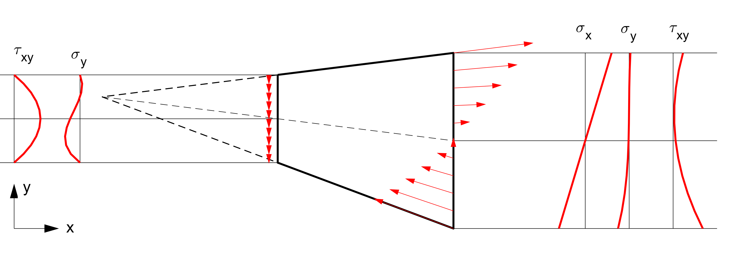
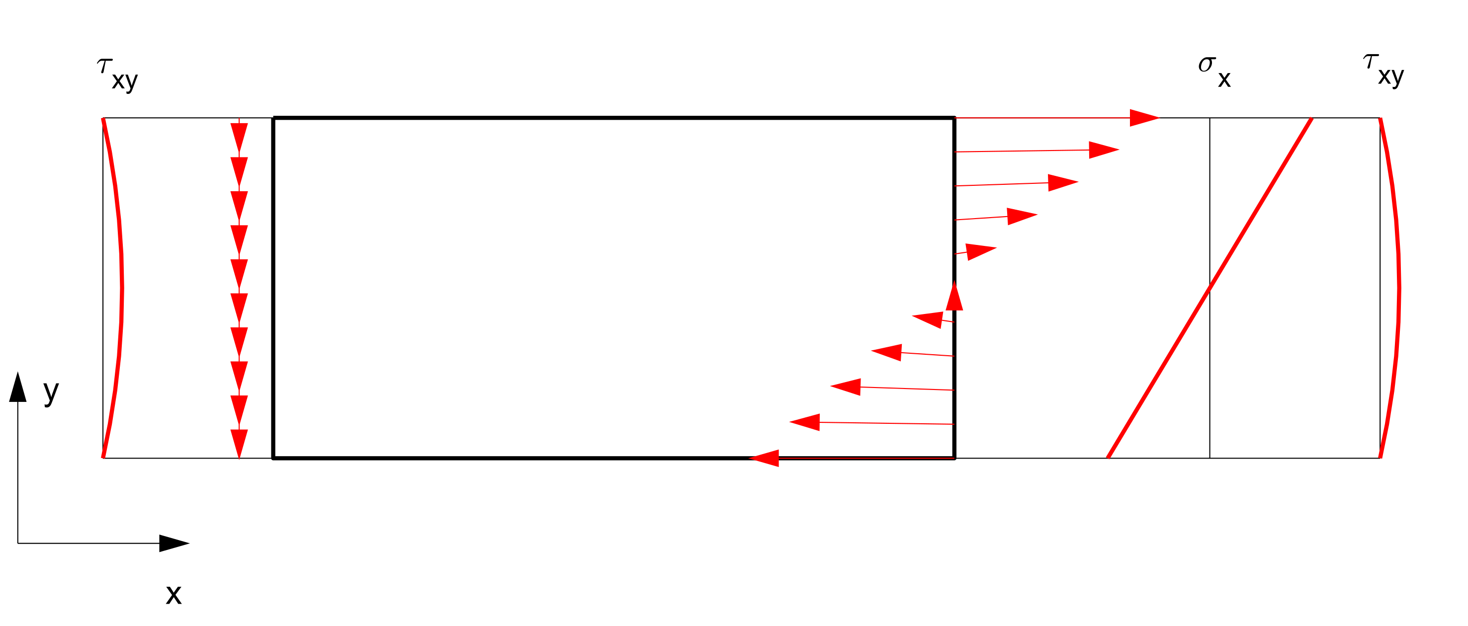
Figure 4: Reducing the problem of a trapezoidal plate to a rectangular one, to which a closed form solution exits.

As a practical example consider a trapezoidal plate acting as a cantilever, loaded on one the end with a vertical force and fully supported on the other end (see top of Figure 4). The load is applied along the vertical side as a distributed load with its intensity governed by a second order polynomial. This setting is similar to how rectangular cantilevers are modelled as shown in the bottom of Figure 4, to which closed-form solutions exist in the literature [14]. Since we may map the two problems into each other through a projective transformation we can transform the exiting solution of the rectangular case to the trapezoidal one, which is the way the solution shown for the trapezoidal case was found. Corollary 2 guarantees that the unsupported and unloaded edges are mapped to unsupported and unloaded edges. The shear directionality of the load is preserved due to Corollary 1. In order to keep the parabolic intensity function of the load we used a collineation that has the line containing the loaded edge as its axis. The deformations of the trapezoidal plate may be calculated from the stress-field and the material properties.

Apart from mapping rectangular problems into trapezoidal ones, another broad set of solved problems that one can rely upon is problems having circular geometry, usually solved with the polar-coordinate form of stress functions. While previous affine transformations could map problems with circular geometry into problems with elliptic geometry, the method presented here can map circles into hyperbolas and parabolas as well, broadening the set of known theoretical solutions even further.

9 Transforming the Airy stress function

The Airy stress function is known [15] to correspond to moments as follows: Let us denote the stress function with $\Psi(p)$ and consider a planar curve $p(s)$ running in the material. Denoting the resultant collected from $s=0$ acting on the material on the left side of the curve (according to the direction given by the parametrization $s$) with $f(s)$, the value of the Airy stress function is the moment value of the resultant with respect to the point on the curve, that is:

$$\Psi(p(s))=\langle p(s),f(s)\rangle$$ (28)

for all $s$. Since we already know how representants of $p$ and $f$ transform, we have

$$\Psi^{\prime}(p^{\prime}(s))=\langle p^{\prime}(s),f^{\prime}(s)\rangle=\frac{\lambda_{F}\text{det}(T)}{\lambda_{p}}\langle Tp(s),T^{-T}f(s)\rangle$$ (29)

$$\Psi^{\prime}(p^{\prime}(s))=\frac{\lambda_{F}\text{det}(T)}{\lambda_{p}}\Psi(p(s)).$$ (30)

Interestingly, this transformation rule may be captured by a three dimensional projective transformation, if we embed the problem into projective three dimensions. We will do this by embedding our $\mathbb{R}^{3}$ based description into $\mathbb{R}^{4}$, the usual $z$ direction of the Euclidean coordinate system corresponding to the point at infinity $u_{3}=(0,0,0,1)^{T}$. For any projective planar transformation represented by matrix $T$ and scalar $\lambda_{F}$ we define an induced projective three dimensional transformation represented by matrix

$$T^{I}:=\begin{bmatrix}T&0_{3}\\ 0_{3}^{T}&\lambda_{F}\text{det}(T)\end{bmatrix}$$ (31)

where $0_{3}$ denotes the $3$ dimensional zero column-vector. If we draw the graph of the Airy stress function, the surface we will constitute of points with representants $\psi(p)=(1,\langle u_{1},p\rangle,\langle u_{2},p\rangle,\Psi(p))^{T}$. Simple calculation shows that

$$T^{I}\psi(p)=(\lambda_{p},\langle u_{1},Tp\rangle,\langle u_{2},Tp\rangle,\lambda_{F}\text{det}(T)\Psi(p))^{T}\sim(1,\langle u_{1},p^{\prime}\rangle,\langle u_{2},p^{\prime}\rangle,\Psi^{\prime}(p^{\prime}))^{T}=\psi^{\prime}(p^{\prime})$$ (32)

meaning the induced map $T^{I}$ represents the transformation rule given in Equation (30).

Figure 5: Left: two surfaces mapped into each other by a projective transformation induced from the horizontal plane. Right: the planar transformation maps the circle to the hyperbola. Where finite points are mapped to finite points the transformation of the mechanical behaviour also makes sense, shown by the two patches and their stresses.

10 Membrane shells

The stress distribution of membrane shells subjected to uniform vertical loading may be thought of as a pair of planar problems connected by Puchers’ equation [9], as follows. Consider a membrane shell corresponding to the surface $H(x,y)$, subjected to uniform vertical loading with intensity $c$; as well as the horizontal projection of the membrane stresses as a planar continuum problem corresponding to the Airy stress function $\Psi(x,y)$. The non-horizontal components of the membrane-equilibrium are equivalent with

$$\frac{\partial^{2}H(x,y)}{\partial x^{2}}\frac{\partial^{2}\Psi(x,y)}{\partial y^{2}}-2\frac{\partial^{2}H(x,y)}{\partial x\partial y}\frac{\partial^{2}\Psi(x,y)}{\partial x\partial y}+\frac{\partial^{2}H(x,y)}{\partial y^{2}}\frac{\partial^{2}\Psi(x,y)}{\partial x^{2}}=-c$$ (33)

which is symmetric in $H$ and $\Psi$, implying the interchangeability of the role of the surfaces. Due to the way the induced maps $T^{I}$ are defined, we have:

Proposition 3.

The Pucher-correspondence of surfaces $H$ and $\Psi$ is invariant under the point-wise effect of the induced maps $T^{I}$.

Proof.

We have to show that for any force present in the three dimensional membrane problem the effect of the induced transformation and the projection to the horizontal plane commute. Consider force $\boldsymbol{F}$ acting at point $\boldsymbol{p}=(x,y,z)$ (Euclidean coordinates). Turning them into projective coordinates $F=(0,\boldsymbol{F})^{T}$ and $p=(1,\boldsymbol{p})^{T}$ the projective line going through them has coordinates [10]

$$p\wedge F=(\langle u_{0},p\rangle\boldsymbol{F}-\langle u_{0},F\rangle\boldsymbol{p},\boldsymbol{p}\times\boldsymbol{F})^{T}$$ (34)

where the first $3$ coordinates are force-components while the second $3$ are moment-components. Denoting the element in the $i$-th row and $j$-th column of $T$ with $T_{ij}$ we may calculate

$$T^{I}p\wedge T^{I}F=\begin{pmatrix}(T_{00}+T_{01}x+T_{02}y)(T_{11}F_{x}+T_{12}F_{y})-(T_{10}+T_{11}x+T_{12}y)(T_{01}F_{x}+T_{02}F_{y})\\ (T_{00}+T_{01}x+T_{02}y)(T_{21}F_{x}+T_{22}F_{y})-(T_{20}+T_{21}x+T_{22}y)(T_{01}F_{x}+T_{02}F_{y})\\ \lambda_{F}\text{det}(T)((T_{00}+T_{01}x+T_{02}y)F_{z}-z(T_{01}F_{x}+T_{02}F_{y}))\\ (T_{10}+T_{11}x+T_{12}y)(T_{21}F_{x}+T_{22}F_{y})-(T_{20}+T_{21}x+T_{22}y)(T_{11}F_{x}+T_{12}F_{y})\\ \lambda_{F}\text{det}(T)((T_{10}+T_{11}x+T_{12}y)F_{z}-z(T_{11}F_{x}+T_{12}F_{y}))\\ \lambda_{F}\text{det}(T)((T_{20}+T_{21}x+T_{22}y)F_{z}-z(T_{21}F_{x}+T_{22}F_{y}))\end{pmatrix}.$$ (35)

Applying $T^{I}$ first then taking the projection means setting the third, fifth and sixth coordinates of the vector on the right hand side to $0$. Projecting first then applying $T^{I}$ means setting $z=0=F_{z}$ on the right hand side. As the two give the same result, we have shown the proposition. ∎

The previously solved affine transformations [9] are naturally contained in this description and form a special case where same planar transformation occurs in every horizontal plane. In general if we slice up a shell with horizontal planes the effect of the transformation might be different in each slice and as such a vertical symmetry axis of the surface is not always preserved under these maps. As we typically have analytical solutions for cases with the vertical axis only, this considerably broadens the set of problems we can describe.

As an example in Figure 5 we show a shell in the shape of a paraboloid of revolution and its image. The planar map maps the base-circle of the paraboloid shell to to a hyperbola, the induced map sends the highest point of the paraboloid to infinity and the image of the paraboloid surface will be a hyperboloid of two sheets. At the same time at points where the image is a finite point the mechanical behaviour of the two shells is also mapped into each other, notably both shell-surfaces coinciding with their stress functions.

References

- [1] J. Plücker. Neue Geometrie des Raumes: gegründet auf die Betrachtungen der geraden Linie als Raumelement. Neue Geometrie des Raumes: gegründet auf die Betrachtung der geraden Linie als Raumelement : zwei Abtheilungen in einem Bande. Teubner, 1868.
- [2] J. Plucker. Fundamental views regarding mechanics. Philosophical Transactions of the Royal Society of London, 156:361–380, 1866.
- [3] J.K. Davidson and K.H. Hunt. Robots and Screw Theory: Applications of Kinematics and Statics to Robotics. Oxford University Press, 2004.
- [4] J. Gallardo-Alvarado. Kinematic Analysis of Parallel Manipulators by Algebraic Screw Theory. Springer International Publishing, 2016.
- [5] R.S. Ball. A Treatise on the Theory of Screws. Cambridge Mathematical Library. Cambridge University Press, 1900.
- [6] Henry Crapo and Walter Whiteley. Statics of frameworks and motions of panel structures: a projective geometric introduction. Structural Topology, 1982, num. 6, 1982.
- [7] William John Macquorn Rankine. Ii. on the mathematical theory of the stability of earth-work and masonry. Proceedings of the Royal Society of London, 8:60–61, 1857.
- [8] N. I. Ostrosablin. Affine transformations of the equations of the linear theory of elasticity. Journal of Applied Mechanics and Technical Physics, 47:564–572, 2006.
- [9] Pál Csonka. Theory and practice of membrane shells. Düsseldorf:VDI Verlag, 1987.
- [10] H. Pottmann and J. Wallner. Computational Line Geometry. Mathematics and Visualization. Springer Berlin Heidelberg, 2001.
- [11] Walter Whiteley. Introduction to structural topology i: Infinitesimal motions and infinitesimal rigidity, 1977.
- [12] Walter Whiteley. Introduction to structural topology ii: Statics and stresses, 1978.
- [13] J. Richter-Gebert. Perspectives on Projective Geometry: A Guided Tour Through Real and Complex Geometry. Springer Berlin Heidelberg, 2011.
- [14] Martin H. Sadd. Elasticity. Academic Press, 2004.
- [15] H. B. Phillips. Stress functions. Journal of Mathematics and Physics, 13(1-4):421–425, 1934.