Neutron decay into a Dark Sector via Leptoquarks

Abstract

In this paper, we extend the Standard Model (SM) scalar sector with scalar leptoquarks (LQ) as a portal to the dark sector to resolve some observational anomalies simultaneously. We introduce LQ coupling to scalar dark matter (DM) to suggest an exotic decay channel for the neutron into scalar DM and an SM anti-neutrino. If the branching ratio of this new neutron decay channel is $1\%$, a long-standing discrepancy in the measured neutron lifetime between two different experimental methods, bottle and beam experiments, can be solved. The mass of the scalar DM produced from neutron decay should be in a narrow range and as a result, its production in the early universe is challenging. We discuss that the freeze-in mechanism can produce this scalar DM in the early universe with the correct relic abundance. Then we show that the model can explain other SM anomalies like the muon $(g-2)$, and $R_{D^{(*)}}$ anomaly simultaneously.

I Introduction

The Standard Model (SM) of particle physics is one of the most successful theories and almost all of its predictions are consistent with experimental results. However, there are some observations that the SM failed to explain. One of the intriguing challenges in particle physics is the neutron lifetime anomaly. It is well-known that the neutron dominantly decays to a proton, an electron, and an anti-electron-neutrino ($\beta$ decay) in the SM framework. The neutron lifetime has been measured by two different methods in experiment, bottle and beam experiments. In the bottle experiment, the ultra-cold neutrons are kept in a container for a time longer than the neutron lifetime, then the remaining neutrons are counted and the neutron lifetime is extracted. The average neutron lifetime from five bottle experiments is Mampe:1993an ; Serebrov:2004zf ; Pichlmaier:2010zz ; Steyerl:2012zz ; Arzumanov:2015tea ,

$$\tau_{n}^{\text{bottle }}=879.6\pm 0.6\mathrm{\leavevmode\nobreak\ s}.$$ (1)

In the second method, the beam experiment, the numbers of the produced protons from the neutron decay are counted and then the neutron lifetime is measured. The average neutron lifetime from two beam experiments is longer than those from the previous method Byrne:1996zz ; Yue:2013qrc ,

$$\tau_{n}^{\text{beam }}=888.0\pm 2.0\mathrm{\leavevmode\nobreak\ s}.$$ (2)

There is a $4\sigma$ discrepancy in neutron lifetime measurements. This discrepancy can be solved if the neutron partially decays to the invisible, for instance, particles in the dark sector (with a branching ratio around $1\%$) Fornal:2018eol ; Davoudiasl:2014gfa ; Barducci:2018rlx ; Ivanov:2018uuk ; Cline:2018ami ; Elahi:2020urr .

On the other hand, numerous observations from galactic to cosmic scales indicate the existence of dark matter (DM) that corresponds to approximately $25\%$ of the energy budget of the Universe. Understanding the nature of DM is one of the longstanding problems in particle physics. Although lots of efforts have been down to unveil the DM nature, its properties are still unknown. For example, we don’t know if the DM is a fermion or a boson, how it interacts (non-gravitationally) with the SM particles, how it was produced in the early universe and the DM mass value (since the wide range of mass is still valid for the DM particle).

It is well-known that the leptoquark (LQ) models are the economical method to address most of the SM anomalies. The LQs can be a scalar or vector and can simultaneously couple to a quark and a lepton. In this paper, the scalar sector of the SM is extended by two scalar LQs ($S^{\alpha}_{1}$ and $S^{\beta}_{1}$) where both have the same quantum number under the SM gauge group but have different baryon and lepton numbers. Also, we add a dark scalar ($\phi$) which is a singlet under the SM. It is shown that by introducing a new coupling between the LQs and the dark scalar, which is a portal between the SM and the dark sectors, the neutron can decay to a dark scalar and an SM anti-neutrino through the scalar LQ mediators. Then it is indicated that the neutron lifetime anomaly can be evaded in a suitable parameter space region.

Since there are severe constraints on the baryon number violation process, we consider the new exotic neutron decay channel with respect to the baryon number Super-Kamiokande:2016exg ; Phillips:2014fgb ; LHCb:2017vth ; SNO:2017pha . So, the new dark scalar carries the baryon and lepton numbers. Furthermore, we show that the dark scalar can be a good DM candidate since it is the lightest particle with the baryon number in the model. On the other hand, the exotic neutron decay channel should be kinematically allowed and at the same time the proton decay should be prevented, so the mass of the scalar DM should be in the narrow range. As a result, the production of such a scalar DM is challenging. However, we show that through the freeze-in scenario, it can be produced in the early universe and its relic density is compatible with the observed abundance of the DM.

In the rest of the paper, we examine other SM anomalies that can be addressed by our model. One of the established anomalies in the SM is related to the high-precision measurement of the magnetic moment of the muon. The SM prediction for the magnetic moment of the muon has around $5.1\sigma$ deviation from the combined result measurement from Brookhaven National Laboratory (BNL) and Fermi National Accelerator Laboratory (FNAL) Aoyama:2020ynm ; Muong-2:2006rrc ; Muong-2:2021ojo ; Muong-2:2021vma ; Muong-2:2023cdq . To alleviate this problem we need new physics with extra particles. Furthermore, the semi-leptonic decays of B-mesons are sensitive to new physics. For example, the BaBar BaBar:2012obs ; BaBar:2013mob , Belle Belle:2015qfa ; Belle:2016dyj ; Belle:2017ilt ; Belle:2019rba , and LHCb LHCb:2015gmp ; LHCb:2017smo ; LHCb:2017rln experiments have measured the $R_{D}$ and $R_{D^{*}}$ observables where they have shown that their result has a deviation from the SM prediction. Although the current uncertainties should be understood better, one can study the new physics effects on these anomalies. Then, we show that our model can solve these SM anomalies simultaneously. It is worth noting that our paper differs from previous studies in the following ways:

• In previous papers, the DM candidate was a fermion particle, but in this paper, the neutron decays to scalar DM.

• We utilized LQ particles as mediator particles due to their intriguing phenomenology and ability to explain multiple anomalies at once.

• We employed the Freeze-in production mechanism during the early universe to account for the DM relic density.

• In this proposed final state of neutron exotic decay, a SM neutrino is produced. Despite their weak interactions, the existence of the neutrinos in the final state could yield a distinct signature compared to previous proposals.

The organization of the paper is as follows. In Section II, we explain the model in detail. In section III the different phenomenological aspects of the model are discussed. Finally, section IV summarises the paper.

II The Model

We extend the SM scalar sector by three new particles. The $S^{\alpha}_{1}$ and $S^{\beta}_{1}$ are the LQ scalars and have the same quantum number under the SM gauge group $(\overline{\mathbf{3}},\mathbf{1},1/3)$, however, they have different baryon and lepton numbers. The third scalar $\phi$ is singlet under the SM gauge symmetries but it carries the baryon and lepton numbers. Table 1 represents all the new scalars with their quantum numbers.

Particles		B		L		$SU(3)_{C}\times SU(2)_{{}_{L}}\times U(1)_{Y}$
$S^{\alpha}_{1}$		$-1/3$		$-1$		($\overline{\mathbf{3}}$     ,   1   ,     1/3)
$S^{\beta}_{1}$		$2/3$		$0$		($\overline{\mathbf{3}}$     ,   1   ,     1/3)
$\phi$		$1$		$1$		(1     ,   1    ,     0)

Table 1: The quantum numbers of the new scalars. The second and third columns show the baryon and lepton numbers, respectively. The last column presents the quantum numbers under the SM gauge groups.

The Lagrangian of the model contains all the particle interactions, and can be written as follows,

$$\mathcal{L}=\mathcal{L}_{{}_{\text{SM}}}+\mathcal{L}_{{}_{\text{LQ, int}}}+\mathcal{L}_{{}_{\text{Scalars}}},$$ (3)

where $\mathcal{L}_{{}_{\rm{SM}}}$ is the SM Lagrangian and $\mathcal{L}_{{}_{\rm{Scalars}}}$ contains all kinetic, mass and interaction terms for scalars. $\mathcal{L}_{{}_{\rm{LQ,int}}}$ indicates the scalar LQ interactions with the SM fermion fields and has the following form Dorsner:2016wpm ,

$$\mathcal{L}_{{}_{\text{LQ, int}}}=y_{ij}^{LL}\bar{Q}_{L}^{Ci,a}S^{\alpha}_{1}\epsilon^{ab}L_{L}^{j,b}+z_{ij}^{LL}\bar{Q}_{L}^{Ci,a}{S^{\beta}_{1}}^{*}\epsilon^{ab}Q_{L}^{j,b}+y_{ij}^{RR}\bar{u}_{R}^{Ci}S^{\alpha}_{1}e_{R}^{j}+\text{ h.c. },$$ (4)

where $Q_{L}\leavevmode\nobreak\ (L_{L})$ indicate the left-handed quark (lepton) doublet and $u_{R}\leavevmode\nobreak\ (e_{R})$ show the right-handed up-type quark (charged lepton). The flavor $(SU(2))$ indices are shown by $i,j=1,2,3\leavevmode\nobreak\ (a,b=1,2)$, and $\epsilon^{ab}=(i\sigma^{2})^{ab}$ that $\sigma^{2}$ is the second Pauli matrix. For the fermion $\psi$, we use the following notation, $\bar{\psi}=\psi^{\dagger}\gamma^{0}$ and $\psi^{C}=C\bar{\psi}^{T}$, where $C=i\gamma^{2}\gamma^{0}$ is the charge conjugation operator. The $y^{LL}$ and $y^{RR}$ are completely arbitrary $3\times 3$ matrices but $z^{LL}$ is a symmetric matrix in flavor space $(z_{ij}^{LL}=z_{ji}^{LL})$. After the contraction in the $SU(2)$ space, we have the following interaction terms for the LQ scalars with the SM fermions,

$$\mathcal{L}_{{}_{\text{LQ, int}}}= - \left(y^{LL}U\right)_{ij}\bar{d}_{L}^{Ci}S^{\alpha}_{1}\nu_{L}^{j}+\left(V^{T}y^{LL}\right)_{ij}\bar{u}_{L}^{Ci}S^{\alpha}_{1}e_{L}^{j}+\left(V^{T}z^{LL}\right)_{ij}\bar{u}_{L}^{Ci}{S^{\beta}_{1}}^{*}d_{L}^{j}$$ (5)

$$- \left(z^{LL}V^{\dagger}\right)_{ij}\bar{d}_{L}^{Ci}{S^{\beta}_{1}}^{*}u_{L}^{j}+y_{ij}^{RR}\bar{u}_{R}^{Ci}S^{\alpha}_{1}e_{R}^{j}+\text{ h.c.}\leavevmode\nobreak\ ,$$

where $U$ is a Pontecorvo-Maki-Nakagawa-Sakata (PMNS) unitary mixing matrix and $V$ is a Cabibbo-Kobayashi-Maskawa (CKM) mixing matrix. All fields in the above equation are in the mass eigenstate basis. Moreover, The scalar Lagrangian for a SM singlet scalar $\phi$ and two other scalars $S^{\alpha}_{1}$ and $S^{\alpha}_{2}$ is given by,

$$\mathcal{L}_{{}_{\text{Scalars}}} = \left|D_{\mu}\phi\right|^{2}-m_{{}_{\phi}}^{2}\left|\phi\right|^{2}+\left|D_{\mu}S^{\alpha}_{1}\right|^{2}-m_{{}_{S^{\alpha}_{1}}}^{2}\left|S^{\alpha}_{1}\right|^{2}+\left|D_{\mu}S^{\beta}_{1}\right|^{2}-m_{{}_{S^{\beta}_{1}}}^{2}\left|S^{\beta}_{1}\right|^{2}-\lambda_{1}\left|S^{\alpha}_{1}\right|^{4}-\lambda_{2}\left|S^{\beta}_{1}\right|^{4}$$

$$- \lambda_{3}\left|\phi\right|^{4}-\lambda_{4}|H|^{2}\left|S^{\alpha}_{1}\right|^{2}-\lambda_{5}|H|^{2}\left|S^{\beta}_{1}\right|^{2}-\lambda_{6}|H|^{2}\left|\phi\right|^{2}-(\mu\leavevmode\nobreak\ S^{\alpha}_{1}({S^{\beta}_{1}})^{*}\phi+\text{ h.c.}),$$

where $H$ is the SM Higgs doublet. The $\lambda_{i}$s are the dimensionless couplings whereas the $\mu$ has a dimension of mass. The last term in the above Lagrangian plays a crucial role in the model because it is a portal between the SM and the dark sectors. As we will explain in the next section the $\phi$ is the lightest particle with the baryon number in our model, as a result, it is stable and can be a good DM candidate.

It is worth mentioning that, in the rest of the paper, for sake of simplicity and in order to resolve some anomalies simultaneously, we consider the following economical flavor ansatz,

$$y_{12}^{LL}\neq 0,\leavevmode\nobreak\ \leavevmode\nobreak\ \leavevmode\nobreak\ \leavevmode\nobreak\ \leavevmode\nobreak\ \leavevmode\nobreak\ y_{33}^{LL}\neq 0,\leavevmode\nobreak\ \leavevmode\nobreak\ \leavevmode\nobreak\ \leavevmode\nobreak\ \leavevmode\nobreak\ \leavevmode\nobreak\ y_{32}^{LL}\neq 0,\leavevmode\nobreak\ \leavevmode\nobreak\ \leavevmode\nobreak\ \leavevmode\nobreak\ \leavevmode\nobreak\ \leavevmode\nobreak\ y_{23}^{LL}\neq 0,\leavevmode\nobreak\ \leavevmode\nobreak\ \leavevmode\nobreak\ \leavevmode\nobreak\ \leavevmode\nobreak\ \leavevmode\nobreak\ y_{32}^{RR}\neq 0,\leavevmode\nobreak\ \leavevmode\nobreak\ \leavevmode\nobreak\ \leavevmode\nobreak\ \leavevmode\nobreak\ \leavevmode\nobreak\ z_{11}^{LL}\neq 0,$$ (6)

and other couplings in the LQ Lagrangian (Eq. 5) are considered to be zero.

III Phenomenology

In this section, we study different phenomenological aspects of our model. In the first subsection III.1, we show how the neutron can decay to a scalar DM and an anti-neutrino via the scalar LQs. We find an appropriate benchmark in our model in which the neutron decay anomaly resolve. The DM production in the early universe and calculating DM relic abundance are presented in the subsection III.2. Then in the subsection III.3, we explain how our setup can eliminate the muon anomalous magnetic moment. In subsection III.4, we indicate that the $R_{D^{(*)}}$ anomaly can be alleviated through our model with the proper parameter space.

III.1 Neutron Decay Anomaly

As we mentioned before, one of the intriguing challenges in particle physics is the neutron lifetime anomaly. In order to evade such an impasse the neutron can partially decay into the dark sector. In our model, the neutron can decay into a scalar DM and an SM anti-neutrino ($n\rightarrow\phi\bar{\nu}$). According to the Lagrangian in Eq. 3 and considering the flavor ansatz in Eq. 6, the following terms have contribution to the exotic neutron decay,

$$\mathcal{L}_{n\rightarrow\phi\bar{\nu}^{i}}=-y_{12}^{LL}U_{2i}\bar{d}_{L}^{C}\nu^{i}_{L}S^{\alpha}_{1}+z_{11}^{LL}V_{11}\bar{u}_{L}^{C}d_{L}(S^{\beta}_{1})^{*}-\mu\leavevmode\nobreak\ S^{\alpha}_{1}({S^{\beta}_{1}})^{*}\phi+\text{h.c.},$$ (7)

where $\nu^{i}_{L}$ can be any mass eigenstate of the SM neutrino. The corresponding Feynman diagram for neutron decay to a scalar DM and an anti-neutrino is shown in Fig. 1(a).

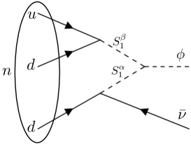
(a) Neutron decay $n\rightarrow\phi\bar{\nu}$

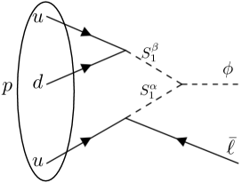
(b) Proton decay $p\rightarrow\phi\bar{\ell}$

Figure 1: The Feynman diagrams contributing to neutron and proton decay.

It is worth mentioning that, there are some constraints on the scalar DM mass $(m_{{}_{\phi}})$. First, for the exotic neutron decay channel to be kinematically allowed, the $\phi$ should be lighter than the neutron. The other bound comes from proton decay. In our model, the proton also can decay to a scalar DM and an anti-muon (according to our flavor ansatz). The Feynman diagram for proton decay is illustrated in Fig. 1(b), and the following Lagrangian terms give rise to proton decays,

$$\mathcal{L}_{p\rightarrow\phi\bar{\mu}}=+y_{12}^{LL}V_{11}\bar{u}_{L}^{C}\mu_{L}S^{\alpha}_{1}+z_{11}^{LL}V_{11}\bar{u}_{L}^{C}d_{L}(S^{\beta}_{1})^{*}-\mu\leavevmode\nobreak\ S^{\alpha}_{1}({S^{\beta}_{1}})^{*}\phi+\text{h.c.}.$$ (8)

To prevent proton decay, the scalar DM mass should be in the following range,

$$m_{p}-m_{\mu}<m_{\phi}<m_{n}\leavevmode\nobreak\ \leavevmode\nobreak\ \leavevmode\nobreak\ \leavevmode\nobreak\ \leavevmode\nobreak\ \leavevmode\nobreak\ \leavevmode\nobreak\ \rightarrow\leavevmode\nobreak\ \leavevmode\nobreak\ \leavevmode\nobreak\ \leavevmode\nobreak\ \leavevmode\nobreak\ \leavevmode\nobreak\ \leavevmode\nobreak\ 832.71\leavevmode\nobreak\ \text{MeV}<m_{\phi}<939.565\leavevmode\nobreak\ \text{MeV}.$$

Moreover, nuclear physics puts other bounds on the $m_{{}_{\phi}}$. The most stringent constraint is required to prevent nuclear decay of ${{}^{9}}\rm{Be}$ Fornal:2018eol ,

$$937.900\leavevmode\nobreak\ \text{MeV}<m_{\phi}<939.565\leavevmode\nobreak\ \text{MeV}.$$

According to the aforementioned limits, we chose $m_{\phi}=938$ MeV as our benchmark. As a result, the $\phi$ is stable since it is the lightest particle with baryon number.

There are some constraints on the (first and second generation) scalar LQs mass from the CMS experiment, where they searched for the single and pair production of scalar LQ. The current bounds require that the mass of the scalar LQ should be larger than 1.36 TeV CMS:2018ncu ; CMS:2018lab ; CMS:2015xzc . So, the scalar LQs are heavier than other particles in the model and they can be integrated out from the Lagrangian. As a result, the effective Lagrangian contributing to the exotic neutron decay is given by,

$$\mathcal{L}_{n\rightarrow\phi\bar{\nu}^{i}}^{\mathrm{eff}}=\kappa^{i}\bar{n}^{C}_{L}\nu^{i}_{L}\phi^{*}+\text{h.c.},$$ (9)

where

$$\kappa_{i}=\frac{\mu\leavevmode\nobreak\ \beta(y_{12}^{LL}U_{2i})(z_{11}^{LL}V_{11})}{m_{{}_{S^{\alpha}_{1}}}^{2}m_{{}_{S^{\beta}_{1}}}^{2}},$$ (10)

that $\beta\cong 0.014\leavevmode\nobreak\ \mathrm{GeV}^{3}$ form lattice QCD Aoki:2017puj . According to the above effective Lagrangian, the exotic neutron decay width to a scalar DM and an anti-neutrino can be calculated as follows,

$$\Delta\Gamma(n\rightarrow\phi\bar{\nu})=\sum_{i}|{\kappa_{i}}|^{2}\frac{1}{16\pi m_{n}^{3}}(m_{n}^{2}-m_{{}_{\phi}}^{2})^{2},$$ (11)

where

$$\sum_{i}|{\kappa_{i}}|^{2}=|\frac{\mu\leavevmode\nobreak\ \beta(y_{12}^{LL})(z_{11}^{LL}V_{11})}{m_{{}_{S^{\alpha}_{1}}}^{2}m_{{}_{S^{\beta}_{1}}}^{2}}|^{2},$$ (12)

and the unitary condition of the PMNS matrix $(\sum_{i}|U_{2i}|^{2}=1)$ is used. To resolve the neutron decay anomaly, the exotic decay width should have the following value Fornal:2018eol ,

$$\Delta\Gamma(n\rightarrow\phi\bar{\nu})=\Gamma_{n}^{\text{bottle }}-\Gamma_{n}^{\text{beam }}\simeq 7.1\times 10^{-30}\leavevmode\nobreak\ \mathrm{GeV}.$$ (13)

Therefore, the following limit is imposed on the combination of the model parameters,

$$|\frac{\mu\leavevmode\nobreak\ y_{12}^{LL}z_{11}^{LL}}{m_{{}_{S^{\alpha}_{1}}}^{2}m_{{}_{S^{\beta}_{1}}}^{2}}|^{2}\simeq 1.8\times 10^{-19}\leavevmode\nobreak\ \rm{GeV}^{-6}.$$ (14)

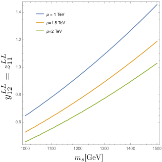
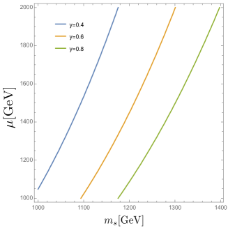
Figure 2: The left panel shows the LQ coupling as a function of the LQ mass for $\mu=$ 1,1.5, and 2 TeV. The right panel shows the $\mu$ coupling as a function of the LQ mass for $y_{12}^{LL}=z_{11}^{LL}=$ 0.4,0.6, and 0.8.

In Fig. 2, we show the accepted values for the LQ mass and LQ coupling with the SM fermion according to the above limit. For simplicity, we assume that $m_{{}_{S^{\alpha}_{1}}}=m_{{}_{S^{\beta}_{1}}}$ and $y_{12}^{LL}=z_{11}^{LL}$. The Left panel shows the LQ coupling as a function of the LQ mass for different values of $\mu$, and the right panel shows the dimensionful coupling $\mu$ as a function of the LQ mass for different values of LQ coupling. According to the figures, the LQ mass around 1.36 TeV and $y_{12}^{LL}=z_{11}^{LL}=$ 0.8 are allowed with dimensionful coupling $\mu$ around the TeV scale. We chose these values as our benchmark.

It is worth mentioning that the neutron star (NS) can put constraints on the models that suggest a new neutron decay channel. The Tolman-Oppenheimer-Volko (TOV) equations determine the NS structure Tolman:1939jz ; Oppenheimer:1939ne . If we integrate the TOV equations from the center of the NS, where the pressure is a constant, to the radius of the NS with zero pressure, we can find the mass of NS as a function of its radius. Also, we can predict the maximum possible mass of the NS. However, to do the above procedure we need to have the Equation of State (EOS) of the NS. The EOS gives the relation between the energy density and the pressure for the NS. The new neutron dark decay channel causes the DM to be thermalized inside the NS and as a result, the EOS would be changed. Ref. McKeen:2018xwc showed that for a non-interacting DM with mass below the neutron mass (to have a kinematically allowed neutron decay channel), the DM produces more energy than the pressure and the EOS of the NS becomes softer. As a result, these models predict maximum mass for neutron stars below $0.7M_{\odot}\$, which is in contradiction with observation. According to the data the current maximum mass for the NS is about $2M_{\odot}\$ Demorest:2010bx ; Antoniadis:2013pzd .

However, Ref. McKeen:2018xwc ; Ellis:2018bkr showed that the DM model with mass greater than $1.2$ GeV or the repulsive self-interacting DM model can escape from these constraints. For instance, if the DM is charged under a new gauge symmetry (U(1) or SU(2)), NS limits can be evaded for a suitable value of dark gauge mediator mass and gauge coupling Cline:2018ami ; Elahi:2020urr . In our model, the neutron decays to a dark scalar and an anti-neutrino $(n\rightarrow\phi\bar{\nu})$. According to the Lagrangian in Eq. II, the scalar DM $(\phi)$ has a repulsive self-interaction term $\lambda_{3}\left|\phi\right|^{4}$ for the $\lambda_{3}>0$. As a result, we can evade NS constraints.

III.2 DM Production

In our model, the DM can be produced through the freeze-in mechanism in early universe Hall:2009bx ; Elahi:2014fsa . In this mechanism, the DM has negligible abundance at the early time, however, some interaction with bath particles can produce the DM. In our case, after the QCD phase transition, the neutron and anti-neutron can decay into $\phi$ and contribute to the DM relic density. Although this contribution is negligible since the obtained relic density for $\phi$ from the neutron decay is four orders of magnitude less than the observed cosmological DM relic Strumia:2021ybk . Another type of interaction that can contribute to $\phi$ relic abundance is $n\pi^{0}\rightarrow\phi\bar{\nu}$ scattering. The number density of the DM ($n_{\phi}$) can be calculated by the Boltzmann equation in the freeze-in scenario,

$$\dot{n}_{\phi}+3n_{\phi}H\approx\int d\Pi_{n}d\Pi_{\pi}d\Pi_{\bar{\nu}}d\Pi_{\phi}(2\pi)^{4}\delta^{4}\left(p_{n}+p_{\pi}-p_{\bar{\nu}}-p_{\phi}\right)|M|_{n\pi\rightarrow\bar{\nu}{\phi}}^{2}f_{n}f_{\pi},$$ (15)

where the $H$ is the Hubble parameter, $d\Pi_{i}=d^{3}p_{i}/(2\pi)^{3}2E_{i}$ are phase space elements and $f_{i}=\left(e^{E_{i}/T}\pm 1\right)^{-1}$ are phase space densities. Assuming the initial particles are in thermal equilibrium we can consider $f_{i}\approx e^{-E_{i}/T}$, and the Boltzmann equation can have the following form Edsjo:1997bg ,

$$\dot{n}_{\phi}+3n_{\phi}H\approx\frac{T}{512\pi^{6}}\int_{(m_{n}+m_{\pi})^{2}}^{\infty}ds\leavevmode\nobreak\ d\Omega\leavevmode\nobreak\ P_{B_{1}B_{2}}\leavevmode\nobreak\ P_{B_{3}{\phi}}\leavevmode\nobreak\ |M|_{n\pi\rightarrow\bar{\nu}{\phi}}^{2}K_{1}(\sqrt{s}/T)/\sqrt{s},$$ (16)

where the $s$ and $T$ are the center of mass energy of the interaction and temperature, respectively. The $K_{1}$ is the first modified Bessel Function of the 2nd kind, and

$$P_{ij}\equiv\frac{\left[s-\left(m_{i}+m_{j}\right)^{2}\right]^{1/2}\left[s-\left(m_{i}-m_{j}\right)^{2}\right]^{1/2}}{2\sqrt{s}}.$$ (17)

The angular integration over the squared amplitude for $n\pi\rightarrow\bar{\nu}\phi$ interaction is as follows,

$$\int d\Omega\leavevmode\nobreak\ |M|_{n\pi\rightarrow\bar{\nu}{\phi}}^{2}=4\pi\lambda^{2}\frac{(s-m^{2}_{\phi})(s+m^{2}_{n}-m^{2}_{\pi})}{2s},$$ (18)

where $\lambda^{2}=|\frac{\mu\leavevmode\nobreak\ \beta\leavevmode\nobreak\ y_{12}^{LL}z_{11}^{LL}g^{2}_{s}}{m_{{}_{S^{\alpha}_{1}}}^{2}m_{{}_{S^{\beta}_{1}}}^{2}}|^{2}$ is the effective coupling and $g_{s}$ is the strong coupling constant. If we use the yield definition, $Y_{\phi}\equiv n_{\phi}/S$ where $S$ is the entropy density, and consider $\dot{T}=-HT$ the left part of Eq. 16 becomes,

$$\dot{n}_{\phi}+3n_{\phi}H=-SHT\frac{dY_{\phi}}{dT},$$ (19)

where $S=2\pi^{2}g_{*}^{S}T^{3}/45$, $H=1.66\sqrt{g_{*}^{\rho}}T^{2}/M_{Pl}$, and $M_{Pl}$ is the non-reduced Planck mass. The $g_{*}^{S,\rho}$ are the effective numbers of degrees of freedom in the bath at the freeze-in temperature for the entropy and energy density, respectively. And finally, the variation of yield is given by,

$$\frac{dY_{\phi}}{dT}\approx\frac{-1}{SHT}\frac{4\pi\lambda^{2}T}{512\pi^{6}}\int_{(m_{n}+m_{\pi})^{2}}^{\infty}\frac{\sqrt{s-(m_{n}+m_{\pi})^{2}}}{2\sqrt{s}}\frac{s-m^{2}_{\phi}}{2\sqrt{s}}\frac{(s-m^{2}_{\phi})(s+m^{2}_{n}-m^{2}_{\pi})}{2s}\frac{K_{1}(\sqrt{s}/T)}{\sqrt{s}}\leavevmode\nobreak\ ds.$$ (20)

By doing the temperature integral with $T_{\rm{min}}=T_{\rm{BBN}}=1\leavevmode\nobreak\ \rm{MeV}$ and $T_{\rm{max}}=\Lambda_{\rm{QCD}}=180\leavevmode\nobreak\ \rm{MeV}$, we can obtain the yield of the DM at present $(Y^{0}_{\phi})$. In this temperature range, the $g_{*}^{S,\rho}$ is $17.25$. Then the DM relic density can be calculated by the following formula,

$$\Omega_{\phi}h^{2}=\frac{m_{\phi}Y^{0}_{\phi}S_{0}}{\rho_{c}/h^{2}},$$ (21)

where $S_{0}=2890/\mathrm{cm}^{3}$ is the entropy density at the present time and $\rho_{c}/h^{2}=1.05\times 10^{-5}\rm{GeV}/\rm{cm}^{3}$ that $\rho_{c}$ is the critical density. As we mentioned before, the model parameters are constrained by the neutron lifetime anomaly (Eq. 14), so the value for $\lambda^{2}=|\frac{\mu\leavevmode\nobreak\ \beta\leavevmode\nobreak\ y_{12}^{LL}z_{11}^{LL}g^{2}_{s}}{m_{{}_{S^{\alpha}_{1}}}^{2}m_{{}_{S^{\beta}_{1}}}^{2}}|^{2}$ is fixed. Therefore, the DM relic density in the model is given by,

$$\Omega_{\phi}h^{2}\approx 0.12(\frac{\lambda}{7.38\times 10^{-11}})^{2},$$ (22)

which is consistent with the Planck collaboration report ($\Omega_{\rm{DM}}h^{2}=0.12$) Planck:2018vyg . It is also noteworthy to mention that, we do a naive calculation here. For more accuracy, someone should consider the following points:

• Some other similar processes can contribute to the $\phi$ relic density such as $p\pi^{0}\rightarrow\phi\bar{\mu}$. However, their contributions to the DM abundance should be in the same order as the $n\pi^{0}\rightarrow\phi\bar{\nu}$ process.

• As reviewed above, the DM yield is strongly dependent on the QCD confinement scale $(T_{\rm{max}}=\Lambda_{\rm{QCD}})$ and the value of the strong coupling constant ($g_{s}$). Since there is a wide range for $\Lambda_{\rm{QCD}}$ from 100 MeV to 1 GeV, the value of the $Y^{0}_{\phi}$ is changing dramatically in this range.

• The effect of the pion structure should also be considered in the effective coupling mentioned above ($\lambda$). Therefore, an extra factor (for example, the pion form factor) should multiply in the $\lambda$, which can reduce the value of the effective coupling by one or two orders of magnitude and change the DM relic density.

However, by considering all of the above-mentioned points, in the worst-case scenario, the $\phi$ scalar can at least contribute to the $10\%$ of the total DM abundance.

III.3 Muon $g-2$

Another long-standing challenge in particle physics is the muon’s anomalous magnetic moment. The updated new world average from Brookhaven National Laboratory Muong-2:2006rrc and Fermi National Accelerator Laboratory Muong-2:2021ojo ; Muong-2:2021vma ; Muong-2:2023cdq for $a_{\mu}=(g-2)_{\mu}/2$ has $5.1\sigma$ deviation from its SM prediction Aoyama:2020ynm ,

$$\delta a_{\mu}=a_{\mu}^{\mathrm{Exp}}-a_{\mu}^{\mathrm{SM}}=(249\pm 48)\times 10^{-11}.$$ (23)

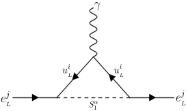
Figure 3: The Feynman diagram contributes to the anomalous magnetic moment of the muon.

It is well-known that the scalar LQ can explain this anomaly Dorsner:2016wpm ; Djouadi:1989md ; Dorsner:2019itg ; Crivellin:2017zlb ; Choi:2018stw ; Cheung:2001ip ; ColuccioLeskow:2016dox ; Crivellin:2020tsz ; Queiroz:2014pra . In our setup, the scalar $S_{1}^{\alpha}$ can contribute to the magnetic moment of the muon and the relevant Feynman diagram is shown in Fig. 3. The related terms from the Lagrangian Eq. 5 are as follows,

$$\mathcal{L}\supset\left(V^{T}y^{LL}\right)_{ij}\bar{u}_{L}^{Ci}S^{\alpha}_{1}e_{L}^{j}+y_{ij}^{RR}\bar{u}_{R}^{Ci}S^{\alpha}_{1}e_{R}^{j}+\text{h.c.},$$ (24)

where the $u^{i}$ is the up-type quark ($u,c,t$) and $e^{j}$ is the charged lepton. According to our economical ansatz (Eq. 6) and because of the large mass of the top quark the following terms involving the top quark and muon have important effects on the $a_{\mu}$,

$$\mathcal{L}\supset y_{32}^{LL}V_{33}\bar{t}_{L}^{C}\mu_{L}S^{\alpha}_{1}+y_{32}^{RR}\bar{t}_{R}^{C}\mu_{R}S^{\alpha}_{1}+\text{h.c.}.$$ (25)

The contribution of the above terms to the anomalous magnetic moment of the muon is given by Djouadi:1989md ,

$$\delta a_{\mu}=-\frac{N_{c}m_{\mu}}{8\pi^{2}m_{{}_{S^{\alpha}_{1}}}^{2}}[m_{\mu}(|y_{32}^{LL}V_{33}|^{2}+|y_{32}^{RR}|^{2})\mathcal{F}(x_{t})+m_{t}\operatorname{Re}[(y_{32}^{RR})^{*}(y_{32}^{LL}V_{33})]\mathcal{G}(x_{t})],$$ (26)

where $m_{\mu}$ and $m_{t}$ indicate the muon and top quark masses, respectively, $x_{t}=m_{t}^{2}/m_{{}_{S^{\alpha}_{1}}}^{2}$, and $N_{c}=3$ is the number of the QCD colors. The definition of $\mathcal{F}(x)$ and $\mathcal{G}(x)$ functions are,

$$\mathcal{F}(x)=\frac{1}{3}f_{S}(x)-f_{F}(x,)$$

$$\mathcal{G}(x)=\frac{1}{3}g_{S}(x)-g_{F}(x),$$ (27)

where

$$f_{S}(x)=\frac{x+1}{4(1-x)^{2}}+\frac{x\log x}{2(1-x)^{3}},\leavevmode\nobreak\ \leavevmode\nobreak\ \leavevmode\nobreak\ \leavevmode\nobreak\ \leavevmode\nobreak\ g_{S}(x)=\frac{1}{x-1}-\frac{\log x}{(x-1)^{2}},$$

$$f_{F}(x)=\frac{x^{2}-5x-2}{12(x-1)^{3}}+\frac{x\log x}{2(x-1)^{4}},\leavevmode\nobreak\ \leavevmode\nobreak\ \leavevmode\nobreak\ \leavevmode\nobreak\ \leavevmode\nobreak\ g_{F}(x)=\frac{x-3}{2(x-1)^{2}}+\frac{\log x}{(x-1)^{3}}.$$

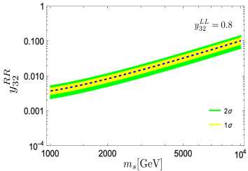
Figure 4: The parameter space of the model ($y_{32}^{RR}$ coupling as a function of LQ’s mass) explains the anomalous magnetic moment of the muon. The yellow and green regions indicate the 1$\sigma$ and 2$\sigma$ levels, respectively. The $y_{32}^{LL}$ value is fixed at 0.8.

As we can see, the first term in Eq. 26 is suppressed by muon mass. The scalar LQ $(S_{1}^{\alpha})$ should have both left-handed and right-handed couplings to generate the second term, which is proportional to top quark mass. As a result of this chirality-enhanced effect and top quark mass, the significant contribution to the $a_{\mu}$ is as follows Crivellin:2017zlb ,

$$\delta a_{\mu}\approx-\frac{N_{c}}{48\pi^{2}m_{{}_{S^{\alpha}_{1}}}^{2}}m_{\mu}m_{t}\operatorname{Re}\left[(y_{32}^{RR})^{*}(y_{32}^{LL}V_{33})\right]\left(7+4\log\left(\frac{m_{t}^{2}}{m_{{}_{S^{\alpha}_{1}}}^{2}}\right)\right).$$ (28)

Fig. 4 displays the parameter space ($y_{32}^{RR}$ coupling as a function of LQ’s mass) where the model can account for the muon $g-2$ anomaly. In this plot, $y_{32}^{LL}$ is fixed at 0.8, based on our benchmark from the neutron lifetime anomaly.

III.4 $R_{D^{(*)}}$ Anomaly

The semi-leptonic decays of B-mesons are sensitive to new physics. The BaBar BaBar:2012obs ; BaBar:2013mob , Belle Belle:2015qfa ; Belle:2016dyj ; Belle:2017ilt ; Belle:2019rba , and LHCb LHCb:2015gmp ; LHCb:2017smo ; LHCb:2017rln experiments have measured the $R_{D}$ and $R_{D^{*}}$ observables where they have shown that their result has a deviation from the SM prediction. Although the current uncertainties should be understood better, one can study the new physics effects on these anomalies. The definition of two anomalous observables are as follows,

$$R_{D} = \frac{\rm{BR}(B\rightarrow D\tau\bar{\nu})}{\rm{BR}(B\rightarrow D\ell\bar{\nu})},$$

$$R_{D^{*}} = \frac{\rm{BR}(B\rightarrow D^{*}\tau\bar{\nu})}{\rm{BR}(B\rightarrow D^{*}\ell\bar{\nu})},$$ (29)

where $\ell=e,\mu$ for BaBar and Bell and $\ell=\mu$ for LHCb. The experimental world averages reporting by Heavy Flavor Averaging Group are HFLAV:2022pwe ,

$$R^{\rm{exp}}_{D} = 0.356\pm 0.029,$$

$$R^{\rm{exp}}_{D^{*}} = 0.284\pm 0.013.$$ (30)

While the SM predictions for these observables are HFLAV:2019otj ,

$$R^{\rm{SM}}_{D} = 0.298\pm 0.004,$$

$$R^{\rm{SM}}_{D^{*}} = 0.254\pm 0.005.$$ (31)

The combination of the experimental result for $R_{D}$ and $R_{D^{*}}$ has a deviation from the SM prediction by about $3\sigma$ WinNT . The effective Lagrangian for $b\rightarrow c\tau\nu^{i}$ is as follows,

$$\mathcal{L}^{\rm{eff}}_{b\rightarrow c\tau\nu^{i}}=-\frac{4G_{F}}{\sqrt{2}}V_{cb}C_{cb}[(\bar{c}_{L}\gamma^{\mu}b_{L})(\bar{\tau}_{L}\gamma_{\mu}\nu^{i}_{L})]+\text{h.c.},$$ (32)

where $G_{F}$ is the Fermi constant and $C_{cb}=1$ in the SM. The new physics can contribute in the above effective operator.

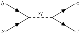
Figure 5: The Feynman diagram contributing to the $b\rightarrow c\tau\nu^{i}$ process and the $R_{D^{(*)}}$ Anomaly.

The LQs are good candidates in order to explain this anomaly. In literature, the different effects of LQs on the B-meson anomalies have been studied extensively Choi:2018stw ; Cheung:2001ip ; Crivellin:2017zlb ; Hiller:2017bzc ; Buttazzo:2017ixm ; Bauer:2015knc ; Chen:2017hir ; Kumar:2018kmr ; Crivellin:2019dwb ; Crivellin:2022mff ; Cai:2017wry . From the Lagrangian in Eq. 5, the terms relevant to the $R_{D^{(*)}}$ anomaly are,

$$\mathcal{L}\supset-\left(y^{LL}U\right)_{ij}\bar{d}_{L}^{Ci}S^{\alpha}_{1}\nu_{L}^{j}+\left(V^{T}y^{LL}\right)_{ij}\bar{u}_{L}^{Ci}S^{\alpha}_{1}e_{L}^{j}+\text{h.c.},$$ (33)

that the $S^{\alpha}_{1}$ LQ can contribute to the $b\rightarrow c\tau\nu^{i}$ process. The relevant Feynman diagram is shown in Fig. 5. According to the economical flavor ansatz (Eq. 6) and after integrating out the scalar LQ, the effective Lagrangian relevant for $b\rightarrow c\tau\nu^{i}$ is given by Dorsner:2016wpm ,

$$\mathcal{L}^{\rm{eff}}_{b\rightarrow c\tau\nu^{i}}=-\frac{4G_{F}}{\sqrt{2}}C^{{}^{\rm{BSM}}}_{cb}[(\bar{c}_{L}\gamma^{\mu}b_{L})(\bar{\tau}_{L}\gamma_{\mu}\nu^{\tau}_{L})]+\text{h.c.},$$ (34)

where $C^{{}^{\rm{BSM}}}_{cb}=\frac{v^{2}(y^{LL}_{33}U_{33})(V^{T}_{22}y^{LL}_{23})^{*}}{4\leavevmode\nobreak\ m_{{}_{S^{\alpha}_{1}}}^{2}}$ that $v$ is the SM Higgs vacuum expectation value. Fig. 6 illustrates the parameter space of the model ($y_{33}^{LL}$ coupling as a function of LQ’s mass) where can explain the $R_{D^{(*)}}$ anomaly. According to our benchmark, the value of the $y_{23}^{LL}$ is fixed at 0.8. This region of parameter space is consistent with the current LHC bound on the LQ mass from $S^{\alpha}_{1}\rightarrow\bar{c}\bar{\tau}$ and $S^{\alpha}_{1}\rightarrow\bar{b}\nu_{\tau}$ decay channels CMS:2017kil .

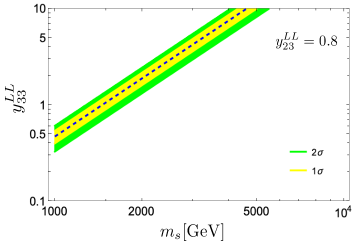
Figure 6: The parameter space of the model ($y_{33}^{LL}$ coupling as a function of LQ’s mass) explains $R_{D^{(*)}}$ anomaly. The yellow and green regions indicate the 1$\sigma$ and 2$\sigma$ levels, respectively. The $y_{23}^{LL}$ value is fixed at 0.8.

IV Summary

In this paper, we introduce a new portal between the standard model (SM) and the dark sectors by scalar leptoquarks (LQ) to resolve some long-standing anomalies simultaneously. The SM predicts the branching ratio of the neutron decay to proton, electron, and anti-electron-neutrino is $100\%$, however, there is an anomaly in the neutron decay width measurements. In the bottle experiments, where the number of the remaining neutrons is counted, the measured neutron lifetime is shorter than the one measured in beam experiments, where the number of the produced protons is counted. This anomaly can be solved, if the neutron decays to invisible (for example, particles in the dark sector) with a branching ratio around $1\%$. We suggest that the neutron decays into a dark scalar ($\phi$) and an SM anti-neutrino by these scalar LQ mediators. The dark scalar is singlet under the SM gauge symmetries but it carries the baryon and lepton numbers since there are severe constraints on the baryon and lepton numbers violation processes. The mass of the $\phi$ should be in the narrow range between 937.9 and 939.565 to satisfy all the current bounds.

The $\phi$ with the aforementioned properties can be a good dark matter (DM) candidate. We showed that the freeze-in mechanism can produce the dark scalar in the early universe and its relic abundance is compatible with the DM relic density measured by the Planck collaboration. Furthermore, we discussed that this model in good parameter space region can explain other SM observational anomalies simultaneously. For instance, the anomalous magnetic moment of the muon, and the $R_{D^{(*)}}$ anomaly can be explained through our model at the same time.

References

- (1) W. Mampe, L. N. Bondarenko, V. I. Morozov, Y. N. Panin, and A. I. Fomin, Measuring neutron lifetime by storing ultracold neutrons and detecting inelastically scattered neutrons, JETP Lett. 57 (1993) 82–87.
- (2) A. Serebrov et. al., Measurement of the neutron lifetime using a gravitational trap and a low-temperature Fomblin coating, Phys. Lett. B 605 (2005) 72–78, [nucl-ex/0408009].
- (3) A. Pichlmaier, V. Varlamov, K. Schreckenbach, and P. Geltenbort, Neutron lifetime measurement with the UCN trap-in-trap MAMBO II, Phys. Lett. B 693 (2010) 221–226.
- (4) A. Steyerl, J. M. Pendlebury, C. Kaufman, S. S. Malik, and A. M. Desai, Quasielastic scattering in the interaction of ultracold neutrons with a liquid wall and application in a reanalysis of the Mambo I neutron-lifetime experiment, Phys. Rev. C 85 (2012) 065503.
- (5) S. Arzumanov, L. Bondarenko, S. Chernyavsky, P. Geltenbort, V. Morozov, V. V. Nesvizhevsky, Y. Panin, and A. Strepetov, A measurement of the neutron lifetime using the method of storage of ultracold neutrons and detection of inelastically up-scattered neutrons, Phys. Lett. B 745 (2015) 79–89.
- (6) J. Byrne and P. G. Dawber, A Revised Value for the Neutron Lifetime Measured Using a Penning Trap, EPL 33 (1996) 187.
- (7) A. T. Yue, M. S. Dewey, D. M. Gilliam, G. L. Greene, A. B. Laptev, J. S. Nico, W. M. Snow, and F. E. Wietfeldt, Improved Determination of the Neutron Lifetime, Phys. Rev. Lett. 111 (2013), no. 22 222501, [1309.2623].
- (8) B. Fornal and B. Grinstein, Dark Matter Interpretation of the Neutron Decay Anomaly, Phys. Rev. Lett. 120 (2018), no. 19 191801, [1801.01124]. [Erratum: Phys.Rev.Lett. 124, 219901 (2020)].
- (9) H. Davoudiasl, Nucleon Decay into a Dark Sector, Phys. Rev. Lett. 114 (2015), no. 5 051802, [1409.4823].
- (10) D. Barducci, M. Fabbrichesi, and E. Gabrielli, Neutral Hadrons Disappearing into the Darkness, Phys. Rev. D 98 (2018), no. 3 035049, [1806.05678].
- (11) A. N. Ivanov, R. Höllwieser, N. I. Troitskaya, M. Wellenzohn, and Y. A. Berdnikov, Neutron dark matter decays and correlation coefficients of neutron -decays, Nucl. Phys. B 938 (2019) 114–130, [1808.09805].
- (12) J. M. Cline and J. M. Cornell, Dark decay of the neutron, JHEP 07 (2018) 081, [1803.04961].
- (13) F. Elahi and M. Mohammadi Najafabadi, Neutron Decay to a Non-Abelian Dark Sector, Phys. Rev. D 102 (2020), no. 3 035011, [2005.00714].
- (14) Super-Kamiokande Collaboration, K. Abe et. al., Search for proton decay via and in 0.31 megaton·years exposure of the Super-Kamiokande water Cherenkov detector, Phys. Rev. D 95 (2017), no. 1 012004, [1610.03597].
- (15) D. G. Phillips, II et. al., Neutron-Antineutron Oscillations: Theoretical Status and Experimental Prospects, Phys. Rept. 612 (2016) 1–45, [1410.1100].
- (16) LHCb Collaboration, R. Aaij et. al., Search for Baryon-Number Violating Oscillations, Phys. Rev. Lett. 119 (2017), no. 18 181807, [1708.05808].
- (17) SNO Collaboration, B. Aharmim et. al., Search for neutron-antineutron oscillations at the Sudbury Neutrino Observatory, Phys. Rev. D 96 (2017), no. 9 092005, [1705.00696].
- (18) T. Aoyama et. al., The anomalous magnetic moment of the muon in the Standard Model, Phys. Rept. 887 (2020) 1–166, [2006.04822].
- (19) Muon g-2 Collaboration, G. W. Bennett et. al., Final Report of the Muon E821 Anomalous Magnetic Moment Measurement at BNL, Phys. Rev. D 73 (2006) 072003, [hep-ex/0602035].
- (20) Muon g-2 Collaboration, B. Abi et. al., Measurement of the Positive Muon Anomalous Magnetic Moment to 0.46 ppm, Phys. Rev. Lett. 126 (2021), no. 14 141801, [2104.03281].
- (21) Muon g-2 Collaboration, T. Albahri et. al., Measurement of the anomalous precession frequency of the muon in the Fermilab Muon g Experiment, Phys. Rev. D 103 (2021), no. 7 072002, [2104.03247].
- (22) Muon g-2 Collaboration, D. P. Aguillard et. al., Measurement of the Positive Muon Anomalous Magnetic Moment to 0.20 ppm, 2308.06230.
- (23) BaBar Collaboration, J. P. Lees et. al., Evidence for an excess of decays, Phys. Rev. Lett. 109 (2012) 101802, [1205.5442].
- (24) BaBar Collaboration, J. P. Lees et. al., Measurement of an Excess of Decays and Implications for Charged Higgs Bosons, Phys. Rev. D 88 (2013), no. 7 072012, [1303.0571].
- (25) Belle Collaboration, M. Huschle et. al., Measurement of the branching ratio of relative to decays with hadronic tagging at Belle, Phys. Rev. D 92 (2015), no. 7 072014, [1507.03233].
- (26) Belle Collaboration, S. Hirose et. al., Measurement of the lepton polarization and in the decay , Phys. Rev. Lett. 118 (2017), no. 21 211801, [1612.00529].
- (27) Belle Collaboration, S. Hirose et. al., Measurement of the lepton polarization and in the decay with one-prong hadronic decays at Belle, Phys. Rev. D 97 (2018), no. 1 012004, [1709.00129].
- (28) Belle Collaboration, G. Caria et. al., Measurement of and with a semileptonic tagging method, Phys. Rev. Lett. 124 (2020), no. 16 161803, [1910.05864].
- (29) LHCb Collaboration, R. Aaij et. al., Measurement of the ratio of branching fractions , Phys. Rev. Lett. 115 (2015), no. 11 111803, [1506.08614]. [Erratum: Phys.Rev.Lett. 115, 159901 (2015)].
- (30) LHCb Collaboration, R. Aaij et. al., Measurement of the ratio of the and branching fractions using three-prong -lepton decays, Phys. Rev. Lett. 120 (2018), no. 17 171802, [1708.08856].
- (31) LHCb Collaboration, R. Aaij et. al., Test of Lepton Flavor Universality by the measurement of the branching fraction using three-prong decays, Phys. Rev. D 97 (2018), no. 7 072013, [1711.02505].
- (32) I. Doršner, S. Fajfer, A. Greljo, J. F. Kamenik, and N. Košnik, Physics of leptoquarks in precision experiments and at particle colliders, Phys. Rept. 641 (2016) 1–68, [1603.04993].
- (33) CMS Collaboration, A. M. Sirunyan et. al., Search for pair production of first-generation scalar leptoquarks at 13 TeV, Phys. Rev. D 99 (2019), no. 5 052002, [1811.01197].
- (34) CMS Collaboration, A. M. Sirunyan et. al., Search for pair production of second-generation leptoquarks at 13 TeV, Phys. Rev. D 99 (2019), no. 3 032014, [1808.05082].
- (35) CMS Collaboration, V. Khachatryan et. al., Search for single production of scalar leptoquarks in proton-proton collisions at , Phys. Rev. D 93 (2016), no. 3 032005, [1509.03750]. [Erratum: Phys.Rev.D 95, 039906 (2017)].
- (36) Y. Aoki, T. Izubuchi, E. Shintani, and A. Soni, Improved lattice computation of proton decay matrix elements, Phys. Rev. D 96 (2017), no. 1 014506, [1705.01338].
- (37) P. D. Group, Workman, and Others, Review of Particle Physics, Progress of Theoretical and Experimental Physics 2022 (08, 2022) 083C01.
- (38) R. C. Tolman, Static solutions of Einstein’s field equations for spheres of fluid, Phys. Rev. 55 (1939) 364–373.
- (39) J. R. Oppenheimer and G. M. Volkoff, On massive neutron cores, Phys. Rev. 55 (1939) 374–381.
- (40) D. McKeen, A. E. Nelson, S. Reddy, and D. Zhou, Neutron stars exclude light dark baryons, Phys. Rev. Lett. 121 (2018), no. 6 061802, [1802.08244].
- (41) P. Demorest, T. Pennucci, S. Ransom, M. Roberts, and J. Hessels, Shapiro Delay Measurement of A Two Solar Mass Neutron Star, Nature 467 (2010) 1081–1083, [1010.5788].
- (42) J. Antoniadis et. al., A Massive Pulsar in a Compact Relativistic Binary, Science 340 (2013) 6131, [1304.6875].
- (43) J. Ellis, G. Hütsi, K. Kannike, L. Marzola, M. Raidal, and V. Vaskonen, Dark Matter Effects On Neutron Star Properties, Phys. Rev. D 97 (2018), no. 12 123007, [1804.01418].
- (44) L. J. Hall, K. Jedamzik, J. March-Russell, and S. M. West, Freeze-In Production of FIMP Dark Matter, JHEP 03 (2010) 080, [0911.1120].
- (45) F. Elahi, C. Kolda, and J. Unwin, UltraViolet Freeze-in, JHEP 03 (2015) 048, [1410.6157].
- (46) A. Strumia, Dark Matter interpretation of the neutron decay anomaly, JHEP 02 (2022) 067, [2112.09111].
- (47) J. Edsjo and P. Gondolo, Neutralino relic density including coannihilations, Phys. Rev. D 56 (1997) 1879–1894, [hep-ph/9704361].
- (48) Planck Collaboration, N. Aghanim et. al., Planck 2018 results. VI. Cosmological parameters, Astron. Astrophys. 641 (2020) A6, [1807.06209]. [Erratum: Astron.Astrophys. 652, C4 (2021)].
- (49) A. Djouadi, T. Kohler, M. Spira, and J. Tutas, (e b), (e t) TYPE LEPTOQUARKS AT e p COLLIDERS, Z. Phys. C 46 (1990) 679–686.
- (50) I. Doršner, S. Fajfer, and O. Sumensari, Muon and scalar leptoquark mixing, JHEP 06 (2020) 089, [1910.03877].
- (51) A. Crivellin, D. Müller, and T. Ota, Simultaneous explanation of and : the last scalar leptoquarks standing, JHEP 09 (2017) 040, [1703.09226].
- (52) S.-M. Choi, Y.-J. Kang, H. M. Lee, and T.-G. Ro, Lepto-Quark Portal Dark Matter, JHEP 10 (2018) 104, [1807.06547].
- (53) K.-m. Cheung, Muon anomalous magnetic moment and leptoquark solutions, Phys. Rev. D 64 (2001) 033001, [hep-ph/0102238].
- (54) E. Coluccio Leskow, G. D’Ambrosio, A. Crivellin, and D. Müller, , lepton flavor violation, and decays with leptoquarks: Correlations and future prospects, Phys. Rev. D 95 (2017), no. 5 055018, [1612.06858].
- (55) A. Crivellin, D. Mueller, and F. Saturnino, Correlating h→+- to the Anomalous Magnetic Moment of the Muon via Leptoquarks, Phys. Rev. Lett. 127 (2021), no. 2 021801, [2008.02643].
- (56) F. S. Queiroz, K. Sinha, and A. Strumia, Leptoquarks, Dark Matter, and Anomalous LHC Events, Phys. Rev. D 91 (2015), no. 3 035006, [1409.6301].
- (57) HFLAV Collaboration, Y. Amhis et. al., Averages of -hadron, -hadron, and -lepton properties as of 2021, 2206.07501.
- (58) HFLAV Collaboration, Y. S. Amhis et. al., Averages of b-hadron, c-hadron, and -lepton properties as of 2018, Eur. Phys. J. C 81 (2021), no. 3 226, [1909.12524].
- (59) https://hflav-eos.web.cern.ch/hflav-eos/semi/winter23_prel/html/RDsDsstar/RDRDs.html.
- (60) G. Hiller and I. Nisandzic, and beyond the standard model, Phys. Rev. D 96 (2017), no. 3 035003, [1704.05444].
- (61) D. Buttazzo, A. Greljo, G. Isidori, and D. Marzocca, B-physics anomalies: a guide to combined explanations, JHEP 11 (2017) 044, [1706.07808].
- (62) M. Bauer and M. Neubert, Minimal Leptoquark Explanation for the , , and Anomalies, Phys. Rev. Lett. 116 (2016), no. 14 141802, [1511.01900].
- (63) C.-H. Chen, T. Nomura, and H. Okada, Excesses of muon , , and in a leptoquark model, Phys. Lett. B 774 (2017) 456–464, [1703.03251].
- (64) J. Kumar, D. London, and R. Watanabe, Combined Explanations of the and Anomalies: a General Model Analysis, Phys. Rev. D 99 (2019), no. 1 015007, [1806.07403].
- (65) A. Crivellin, D. Müller, and F. Saturnino, Flavor Phenomenology of the Leptoquark Singlet-Triplet Model, JHEP 06 (2020) 020, [1912.04224].
- (66) A. Crivellin, B. Fuks, and L. Schnell, Explaining the hints for lepton flavour universality violation with three S2 leptoquark generations, JHEP 06 (2022) 169, [2203.10111].
- (67) Y. Cai, J. Gargalionis, M. A. Schmidt, and R. R. Volkas, Reconsidering the One Leptoquark solution: flavor anomalies and neutrino mass, JHEP 10 (2017) 047, [1704.05849].
- (68) CMS Collaboration, A. M. Sirunyan et. al., Search for the pair production of third-generation squarks with two-body decays to a bottom or charm quark and a neutralino in proton–proton collisions at = 13 TeV, Phys. Lett. B 778 (2018) 263–291, [1707.07274].