Secret Key Generation for IRS-Assisted Multi-Antenna Systems: A Machine Learning-Based Approach

Abstract

Physical-layer key generation (PKG) based on wireless channels is a lightweight technique to establish secure keys between legitimate communication nodes. Recently, intelligent reflecting surfaces (IRSs) have been leveraged to enhance the performance of PKG in terms of secret key rate (SKR), as it can reconfigure the wireless propagation environment and introduce more channel randomness. In this paper, we investigate an IRS-assisted PKG system, taking into account the channel spatial correlation at both the base station (BS) and the IRS. Based on the considered system model, the closed-form expression of SKR is derived analytically considering correlated eavesdropping channels. Aiming to maximize the SKR, a joint design problem of the BS’s precoding matrix and the IRS’s phase shift vector is formulated. To address this high-dimensional non-convex optimization problem, we propose a novel unsupervised deep neural network (DNN)-based algorithm with a simple structure. Different from most previous works that adopt iterative optimization to solve the problem, the proposed DNN-based algorithm directly obtains the BS precoding and IRS phase shifts as the output of the DNN. Simulation results reveal that the proposed DNN-based algorithm outperforms the benchmark methods with regard to SKR.

I Introduction

Along with the surge in data traffic envisioned by sixth generation (6G) communication, data security risks emerge due to the broadcast nature of wireless transmissions [2, 3]. Conventional cryptographic approaches rely on either asymmetric or symmetric encryption for achieving data confidentiality. Asymmetric cryptography, also known as public key cryptography (PKC), can be used for data encryption and key distribution. The latter can share keys for symmetric encryption, e.g., advanced encryption standard (AES). However, PKC is computationally complicated and requires public key infrastructure for the distribution of keys. Therefore, conventional cryptographic approaches are challenging to be applied to mobile communication networks and resource-constrained Internet of Things (IoT).

In this context, physical-layer key generation (PKG) has been proposed as a lightweight technique that does not rely on conventional cryptographic schemes and is information-theoretically secure [4]. PKG utilizes the reciprocity of wireless channels during the channel coherent time to generate symmetric keys from bidirectional channel probings. The spatial decorrelation and channel randomness ensure the security of the generated keys. More specifically, spatial decorrelation ensures that eavesdroppers cannot generate the same keys as legitimate communicating nodes, and channel randomness prevents the generated keys from dictionary attacks.

Although the effectiveness of PKG has been demonstrated both theoretically and experimentally [5, 6, 7, 8, 9], PKG may face serious challenges in harsh propagation environments. The transmission link between two legitimate nodes may experience non-line-of-sight (NLoS) propagation conditions due to the effects of blockages. In this case, the channel estimation will suffer from a low signal-to-noise ratio (SNR), resulting in a high bit disagreement rate (BDR) and low secret key rate (SKR). Besides, in a quasi-static environment that lacks randomness, the achievable SKR is limited due to low channel entropy [4, 10].

To address these challenges, a new paradigm, called intelligent reflecting surface (IRS), offers attractive solutions. IRS consists of low-cost passive reflecting elements that can dynamically adjust their amplitudes and/or phases to reconfigure the wireless propagation environments in an energy-efficient manner [11, 12]. The reflection channels provided by IRS are capable of enhancing the received signals at legitimate users and introducing rich channel randomness. There have been several works exploring the application of IRS in PKG [13, 14, 15, 16]. The work in [13] improved the SKR of an IRS-aided single-antenna system by randomly configuring the IRS’s phase shifts, in which closed-form expressions of the lower and upper bounds of the SKR were provided. In [14], a practical prototype of IRS-assisted PKG system was implemented using commodity Wi-Fi transceivers, which demonstrated that the randomly configured IRS can boost the key generation rate while ensuring the randomness of the generated keys. To further improve the SKR, some works developed optimization algorithms to configure the IRS’s phase shifts. In [15], the IRS phase shifts were optimized to maximize the minimum achievable SKR. Successive convex approximation was adopted to address the non-convex optimization objective. In [16], the authors considered a multi-user scenario and designed IRS phase shifts to maximize the sum SKR. Nevertheless, these works only considered the optimization of IRS phase shifts in a single-antenna scenario, and thus cannot be applied to multi-antenna systems that require a joint design of multi-antenna precoding and IRS phase shifts.

Multi-antenna technique has been a key enabler of fifth generation (5G) and beyond wireless communication networks [17, 18]. Therefore, securing IRS-assisted multi-antenna transmissions using PKG becomes an important topic. Compared to IRS-assisted PKG efforts in single-antenna scenarios, there is limited work investigating PKG in IRS-assisted multi-antenna systems [19, 20]. In [19], the authors maximized the minimum SKR by jointly optimizing the transmit and the reflective beamforming through a block successive upper-bound minimization-based algorithm. The unit pilot length was adopted for both uplink and downlink channel probings, which simplified the analysis but limited the SKR. In [20], the BS precoding and IRS phase shift matrices were jointly designed using fine-grained channel estimation. However, the analysis of correlated eavesdropping channels was overlooked. Generally, the optimal configuration of IRS is a complex non-convex optimization problem. This problem is exacerbated in multi-antenna systems that require a joint optimization of transmit precoding and reflection beamforming. The existing works rely on iterative optimization algorithms with a high computational complexity, which is difficult to be deployed in practice.

Recently, machine learning has emerged as one of the key techniques to address mathematically intractable non-convex optimization problems [21, 22]. There have been research efforts [23, 24, 25, 26] leveraging machine learning to optimize IRS reflecting beamforming with the aim of maximizing downlink transmission rates. A recent work [27] proposed a machine learning-based adaptive quantization method to balance key generation rate and BDR in an IRS-aided single-antenna system, where the IRS phase shifts were configured using iterative optimization. Up to now, the employment of machine learning to optimize IRS phase shifts in an IRS-aided PKG system has not been investigated.

To the best of our knowledge, this is the first attempt to exploit machine learning in jointly optimizing the transmit precoding and IRS reflection beamforming for maximizing the SKR in an IRS-assisted multi-antenna system. Our major contributions are summarized as follows:

• We propose a new PKG framework for an IRS-assisted multi-antenna system and derive the closed-form expression of SKR considering correlated eavesdropping channels and spatial correlation among BS antennas and IRS elements.

• We formulate the optimization problems of SKR maximization in the absence and presence of eavesdropper channel statistics, respectively. Then water-filling algorithm-based baseline solutions are developed to jointly design the BS’s precoding matrix and the IRS’s phase shift vector.

• We novelly propose to obtain the optimal configuration of BS precoding and IRS phase shifts by using unsupervised deep neural networks (DNNs), referred to as “PKG-Net”. The proposed PKG-Net can deal with different transmit power levels and channel statistics parameters. Simulations demonstrate that the proposed PKG-Net can achieve a higher SKR than other benchmark methods. Compared with the water-filling algorithm-based baseline solution, the proposed PKG-Net has a significantly lower computational complexity.

Different from our previous work [1], where the eavesdropping channels are assumed to be uncorrelated with the legitimate channels, in this paper, we considerably extend the system to a more general scenario in the presence of correlated eavesdropping channels. Moreover, the DNN developed in [1] only has generalization ability to different user locations. In this paper, we further extend the generalization ability of PKG-Net to different transmission powers and channel statistics.

The rest of this paper is organized as follows. In Section II, we present the system model. In Section III, we derive the expression of SKR. The problem formulation is presented in Section IV. Then we propose a water-filling algorithm-based baseline solution in Section V. A machine-learning-based method is developed in Section VI. Our simulation results and analysis are given in Section VII. Finally, Section VIII concludes this paper.

Notations: In this paper, scalars are represented by italic letters, vectors by boldface lower-case letters, and matrices by boldface uppercase letters. $\mathbf{V}^{T}$, $\mathbf{V}^{H}$ and $\mathbf{V}^{*}$ are the transpose, conjugate transpose and conjugate of a matrix $\mathbf{V}$, respectively. $\mathbb{E}\{\cdot\}$ is the statistical expectation. $\mod(\cdot)$ and $\lfloor\cdot\rfloor$ denote modulus operator and floor function, respectively. $[\mathbf{V}]_{i,j}$ denotes the $(i,j)$-th element of a matrix $\mathbf{V}$. $\mathcal{CN}(\mu,\sigma^{2})$ represents a circularly symmetric complex Gaussian distribution with mean $\mu$ and variance $\sigma^{2}$. $\text{diag}(\mathbf{v})$ is a diagonal matrix with the entries of $\mathbf{v}$ on its main diagonal and $\text{vec}(\mathbf{V})$ is the vectorization of a matrix $\mathbf{V}$. $\mathbb{C}^{A\times B}$ represents the sapce of a complex matrix with size $A\times B$. $||\cdot||_{F}$ denotes the Frobenius norm. $\odot$ and $\otimes$ are the Hadamard product and Kronecker product, respectively.

II System Model

II-A System Overview

We consider an IRS-assisted multi-antenna system as shown in Fig. 1, which contains a multi-antenna BS, Alice, a single-antenna user equipment (UE), Bob, a single-antenna eavesdropper, Eve, and an IRS. We assume that the BS is a uniform linear array with $M$ antennas, and the IRS is a uniform planar array, which consists of $L=L_{\mathrm{H}}\times L_{\mathrm{V}}$ passive reflecting elements with $L_{\mathrm{H}}$ elements per row and $L_{\mathrm{V}}$ elements per column. To secure the communication, Alice and Bob perform PKG with the assistance of the IRS.

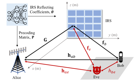
Figure 1: System model.

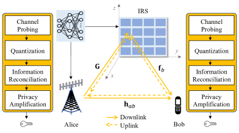
Figure 2: PKG protocol.

As shown in Fig. 2, the PKG protocol consists of four phases: channel probing, quantization, information reconciliation and privacy amplification. During the channel probing phase, Alice and Bob perform bidirectional channel measurements by transmitting pilot signals to each other. We assume a time-division duplexing (TDD) protocol, and thus Alice and Bob can observe reciprocal channel information. During the quantization phase, Alice and Bob quantize the channel observations into binary key bits. Then the disagreed key bits are corrected by information reconciliation and the leaked information is eliminated by privacy amplification [4]. In this paper, we focus on the channel probing phase, because the channel measurements with IRS and multi-antenna configuration need to be optimized.

II-B Channel Model

We denote the Alice-IRS, IRS-Bob (IRS-Eve), Alice-Bob (Alice-Eve) and Bob-Eve channels by $\mathbf{G}\in\mathbb{C}^{M\times L}$, $\mathbf{f}_{b}~{}(\mathbf{f}_{e})\in\mathbb{C}^{L\times 1}$, $\mathbf{h}_{ab}~{}(\mathbf{h}_{ae})\in\mathbb{C}^{M\times 1}$ and $h_{be}\in\mathbb{C}^{1\times 1}$, respectively. All the channels are modelled as spatially correlated Rician fading channels. To be specific, we have

$$\mathbf{G} =\mathbf{G}^{\mathrm{L}}+\mathbf{G}^{\mathrm{NL}},$$ (1)

$$\mathbf{f}_{i} =\mathbf{f}_{i}^{\mathrm{L}}+\mathbf{f}_{i}^{\mathrm{NL}},i\in\{b,e\},$$ (2)

$$\mathbf{h}_{ai} =\mathbf{h}_{ai}^{\mathrm{L}}+\mathbf{h}_{ai}^{\mathrm{NL}},i\in\{b,e\},$$ (3)

$$h_{be} =h_{be}^{\mathrm{L}}+h_{be}^{\mathrm{NL}},$$ (4)

where $\mathbf{G}^{\mathrm{L}}$, $\mathbf{f}_{i}^{\mathrm{L}}$, $\mathbf{h}_{ai}^{\mathrm{L}}$ and $h_{be}^{\mathrm{L}}$ are the line-of-sight (LoS) components of ${\mathbf{G}}$, ${\mathbf{f}_{i}}$, ${\mathbf{h}}_{ai}$ and $h_{be}$, respectively, and $\mathbf{G}^{\mathrm{NL}}$, $\mathbf{f}_{i}^{\mathrm{NL}}$, $\mathbf{h}_{ai}^{\mathrm{NL}}$ and $h_{be}^{\mathrm{NL}}$ are the non-line-of-sight (NLoS) components of ${\mathbf{G}}$, ${\mathbf{f}_{i}}$, ${\mathbf{h}}_{ai}$ and $h_{be}$, respectively. The LoS components are deterministic channels that depend on the locations of Alice, Bob and Eve, while the NLoS components are modelled as spatially correlated Rayleigh fading channels. The NLoS components are further defined as

$$\mathbf{G}^{\mathrm{NL}} =\mathbf{R}_{\mathrm{B}}^{\frac{1}{2}}\widetilde{\mathbf{G}}\mathbf{R}_{\mathrm{I}}^{\frac{1}{2}},$$ (5)

$$\mathbf{f}_{i}^{\mathrm{NL}} =\mathbf{R}_{\mathrm{I}}^{\frac{1}{2}}\widetilde{\mathbf{f}}_{i},i\in\{b,e\},$$ (6)

$$\mathbf{h}_{ai}^{\mathrm{NL}} =\mathbf{R}_{\mathrm{B}}^{\frac{1}{2}}\widetilde{\mathbf{h}}_{ai},i\in\{b,e\},$$ (7)

where $\mathbf{R}_{\mathrm{B}}\in\mathbb{R}^{M\times M}$ and $\mathbf{R}_{\mathrm{I}}\in\mathbb{R}^{L\times L}$ are the spatial correlation matrices at the BS and IRS, respectively, $\widetilde{\mathbf{G}}\in\mathbb{C}^{M\times L}$, $\widetilde{\mathbf{f}}_{i}\in\mathbb{C}^{L\times 1}$ and $\widetilde{\mathbf{h}}_{ai}\in\mathbb{C}^{M\times 1}$ have i.i.d. entries $\mathcal{CN}\left(0,\frac{\beta_{\mathrm{G}}}{1+\kappa_{\mathrm{G}}}\right)$, $\mathcal{CN}\left(0,\frac{\beta_{\mathrm{f}_{i}}}{1+\kappa_{\mathrm{f}_{i}}}\right)$ and $\mathcal{CN}\left(0,\frac{\beta_{\mathrm{h}_{ai}}}{1+\kappa_{\mathrm{h}_{ai}}}\right)$, respectively, in which $\beta_{\mathrm{G}}$, $\beta_{\mathrm{f}_{i}}$ and $\beta_{\mathrm{h}_{ai}}$ are the path loss of ${\mathbf{G}}$, ${\mathbf{f}_{i}}$ and ${\mathbf{h}}_{ai}$, respectively, and $\kappa_{\mathrm{G}}$, $\kappa_{\mathrm{f}_{i}}$ and $\kappa_{\mathrm{h}_{ai}}$ are the Rician factors of ${\mathbf{G}}$, ${\mathbf{f}_{i}}$ and ${\mathbf{h}}_{ai}$, respectively. Moreover, $h_{be}^{\mathrm{NL}}\sim\mathcal{CN}\left(0,\frac{\beta_{\mathrm{h}_{be}}}{1+\kappa_{\mathrm{h}_{be}}}\right)$, where $\beta_{\mathrm{h}_{be}}$ and $\kappa_{\mathrm{h}_{be}}$ are the path loss and Rician factor of $\mathrm{h}_{be}$, respectively. Without loss of generality, we assume that the direct channels are in NLOS conditions, i.e., $\kappa_{\mathrm{h}_{ai}}=0$, and that $\kappa_{\mathrm{G}}=\kappa_{\mathrm{f}_{i}}=\kappa$.

In practice, there exist spatial correlations among BS antennas and IRS elements. For simplicity, we adopt the spatial correlation model in isotropic scattering environments, where the ($n,m$)-th element of the spatial correlation matrix at the IRS is given by [28]

$$[\mathbf{R}_{\mathrm{I}}]_{n,m}=\frac{\sin(\frac{2\pi}{\lambda}||\mathbf{u}_{n}-\mathbf{u}_{m}||_{2})}{\frac{2\pi}{\lambda}||\mathbf{u}_{n}-\mathbf{u}_{m}||_{2}},~{}n,m=1,\dots,L,$$ (8)

where $\lambda$ is the wavelength, and $\mathbf{u}_{n}$ denotes the location of the $n$-th element and is computed as $\mathbf{u}_{n}=\left[0,y_{n}\Delta,z_{n}\Delta\right]^{T}$, in which $y_{n}=\mod(n-1,L_{\mathrm{H}})$ and $z_{n}=\left\lfloor(n-1)/L_{\mathrm{H}}\right\rfloor$ are the horizontal and vertical indices of the $n$-th element, respectively, and $\Delta$ is the element spacing. The spatial correlation matrix at the BS is represented by $\mathbf{R}_{\mathrm{B}}$ with the ($n,m$)-th element given by

$$[\mathbf{R}_{\mathrm{B}}]_{m,n}=\eta^{|m-n|},$$ (9)

where $\eta$ is the correlation coefficient among BS antennas [29].

II-C IRS Assisted Channel Probing

The channel probing is composed of bidirectional measurements, i.e., uplink and downlink probings. We assume a passive Eve who intends to eavesdrop on the information transmitted through legitimate channels.

II-C1 Uplink Channel Probing

During the uplink phase, Bob transmits a pilot signal $s_{u}\in\mathbb{C}^{1\times 1}$ to Alice. The received signals at Alice and Eve are given by

$$\mathbf{y}_{a} =\sqrt{P_{b}}\left(\mathbf{h}_{ab}+\mathbf{G}\mathbf{\Theta}\mathbf{f}_{b}\right)s_{u}+\mathbf{n}_{a},$$ (10)

$$y_{be} =\sqrt{P_{b}}\left(h_{be}+\mathbf{f}_{e}^{T}\mathbf{\Theta}\mathbf{f}_{b}\right)s_{u}+n_{e}^{u},$$ (11)

respectively, where $\mathbf{y}_{a}\in\mathbb{C}^{M\times 1}$, $P_{b}$ is the transmit power of Bob, $\mathbf{\Theta}=\text{diag}\left(e^{j\theta_{1}},e^{j\theta_{2}},\dots,e^{j\theta_{L}}\right)$ denotes the IRS phase shift matrix with $\theta_{l}\in[0,2\pi)$ for the $l$-th element, $\mathbf{n}_{a}\in\mathbb{C}^{M\times 1}$ is the complex Gaussian noise vector at Alice and $n_{e}^{u}$ is the complex Gaussian noise at Eve. Then Alice applies the precoding matrix $\mathbf{P}\in\mathbb{C}^{M\times N}$, where $N$ is the pilot length, to $\mathbf{y}_{a}$ and obtains

$$\bar{\mathbf{y}}_{a}=\sqrt{P_{b}}\mathbf{P}^{T}\left(\mathbf{h}_{ab}+\mathbf{G}\mathbf{\Theta}\mathbf{f}_{b}\right)s_{u}+\mathbf{P}^{T}\mathbf{n}_{a}.$$ (12)

After the least square (LS) channel estimation, the uplink channels at Alice and Eve are estimated as

$$\widehat{\mathbf{y}}_{a} =\sqrt{P_{b}}\mathbf{P}^{T}\left(\mathbf{h}_{ab}+\mathbf{G}\mathbf{\Theta}\mathbf{f}_{b}\right)+\mathbf{P}^{T}\mathbf{n}_{a}s_{u}^{*},$$ (13)

$$\widehat{y}_{be} =\sqrt{P_{b}}\left(h_{be}+\mathbf{f}_{e}^{T}\mathbf{\Theta}\mathbf{f}_{b}\right)+n_{e}^{u}s_{u}^{*}.$$ (14)

II-C2 Downlink Channel Probing

During the downlink phase, Alice transmits a pilot signal of length $N$, $\mathbf{S}_{d}\in\mathbb{C}^{N\times N}$, with $\mathbf{S}_{d}^{H}\mathbf{S}_{d}=\mathbf{I}_{N}$ to Bob. The received signals at Bob and Eve are given by

$$\mathbf{y}_{b} =\left(\mathbf{h}_{ab}+\mathbf{G}\mathbf{\Theta}\mathbf{f}_{b}\right)^{T}\mathbf{P}\mathbf{S}_{d}^{H}+\mathbf{n}_{b},$$ (15)

$$\mathbf{y}_{ae} =\left(\mathbf{h}_{ae}+\mathbf{G}\mathbf{\Theta}\mathbf{f}_{e}\right)^{T}\mathbf{P}\mathbf{S}_{d}^{H}+\mathbf{n}_{e}^{d},$$ (16)

respectively, where $\mathbf{y}_{b},\mathbf{y}_{ae}\in\mathbb{C}^{1\times N}$, $\mathbf{n}_{b}\in\mathbb{C}^{1\times N}$ is the complex Gaussian noise vector at Bob and $\mathbf{n}_{e}^{d}\in\mathbb{C}^{1\times N}$ is the complex Gaussian noise vector at Eve. After LS channel estimation, the downlink channels at Bob and Eve are estimated as

$$\widehat{\mathbf{y}}_{b} ={\mathbf{y}}_{b}\mathbf{S}_{d}\left(\mathbf{S}_{d}^{H}\mathbf{S}_{d}\right)^{-1}=\left(\mathbf{h}_{ab}+\mathbf{G}\mathbf{\Theta}\mathbf{f}_{b}\right)^{T}\mathbf{P}+\mathbf{n}_{b}\mathbf{S}_{d},$$ (17)

$$\widehat{\mathbf{y}}_{ae} ={\mathbf{y}}_{ae}\mathbf{S}_{d}\left(\mathbf{S}_{d}^{H}\mathbf{S}_{d}\right)^{-1}=\left(\mathbf{h}_{ae}+\mathbf{G}\mathbf{\Theta}\mathbf{f}_{e}\right)^{T}\mathbf{P}+\mathbf{n}_{e}^{d}\mathbf{S}_{d}.$$ (18)

Then Bob and Eve transpose $\widehat{\mathbf{y}}_{b}$ and $\widehat{\mathbf{y}}_{ae}$, respectively, and obtain

$$\widehat{\mathbf{y}}_{b}^{T} =\mathbf{P}^{T}\left(\mathbf{h}_{ab}+\mathbf{G}\mathbf{\Theta}\mathbf{f}_{b}\right)+\mathbf{S}_{d}^{T}\mathbf{n}_{b}^{T},$$ (19)

$$\widehat{\mathbf{y}}_{ae}^{T} =\mathbf{P}^{T}\left(\mathbf{h}_{ae}+\mathbf{G}\mathbf{\Theta}\mathbf{f}_{e}\right)+\mathbf{S}_{d}^{T}\left(\mathbf{n}_{e}^{d}\right)^{T}.$$ (20)

To fully extract the randomness from BS antennas, we set $N=M$ in this paper.

PKG relies on the randomness of channels, and thus the deterministic LOS components do not contribute to the SKR [30]. After estimating and removing the LOS components, the uplink channel observations are expressed as

$$\widetilde{\mathbf{y}}_{a} =\sqrt{P_{b}}\mathbf{P}^{T}\left(\mathbf{h}_{ab}^{\mathrm{NL}}+\mathbf{G}^{\mathrm{NL}}\mathbf{\Theta}\mathbf{f}_{b}^{\mathrm{NL}}\right)+\mathbf{P}^{T}\mathbf{n}_{a}s_{u}^{*},$$ (21)

$$\widetilde{y}_{be} =\sqrt{P_{b}}\left(h_{be}^{\mathrm{NL}}+\left(\mathbf{f}_{e}^{\mathrm{NL}}\right)^{T}\mathbf{\Theta}\mathbf{f}_{b}^{\mathrm{NL}}\right)+n_{e}^{u}s_{u}^{*},$$ (22)

and the downlink channel observations are expressed as

$$\widetilde{\mathbf{y}}_{b}^{T} =\mathbf{P}^{T}\left(\mathbf{h}_{ab}^{\mathrm{NL}}+\mathbf{G}^{\mathrm{NL}}\mathbf{\Theta}\mathbf{f}_{b}^{\mathrm{NL}}\right)+\mathbf{S}_{d}^{T}\mathbf{n}_{b}^{T},$$ (23)

$$\widetilde{\mathbf{y}}_{ae}^{T} =\mathbf{P}^{T}\left(\mathbf{h}_{ae}^{\mathrm{NL}}+\mathbf{G}^{\mathrm{NL}}\mathbf{\Theta}\mathbf{f}_{e}^{\mathrm{NL}}\right)+\mathbf{S}_{d}^{T}\left(\mathbf{n}_{e}^{d}\right)^{T}.$$ (24)

III Secret Key Rate

SKR is defined as the maximum number of secret key bits that can be extracted from a channel observation. The exact expression of SKR given the correlated eavesdropping channel is still an open problem. In this section, we derive a closed-form expression for the lower bound of SKR in the IRS-assisted multi-antenna system. According to [31], the lower bound of SKR is expressed as follows:

$$R_{\mathrm{sk}}\left(\widetilde{\mathbf{y}}_{a},\widetilde{\mathbf{y}}_{b},\widetilde{\mathbf{y}}_{ae},\widetilde{y}_{be}\right)\!=\!\mathrm{max}\big{\{} I\left(\widetilde{\mathbf{y}}_{a};\widetilde{\mathbf{y}}_{b}^{T}\right)\!-\!I\left(\widetilde{\mathbf{y}}_{a};\widetilde{\mathbf{y}}_{ae}^{T},\widetilde{y}_{be}\right),$$

$$I\left(\widetilde{\mathbf{y}}_{a};\widetilde{\mathbf{y}}_{b}^{T}\right)\!-\!I\left(\widetilde{\mathbf{y}}_{b};\widetilde{\mathbf{y}}_{ae}^{T},\widetilde{y}_{be}\right)\big{\}},$$ (25)

where $I(X;Y)$ denotes the mutual information between random variables $X$ and $Y$. We assume that Eve gets as close as possible to Bob to maximize the correlation between his channel observation $\widetilde{\mathbf{y}}_{ae}^{T}$ and the legitimate channels. As such, $\widetilde{y}_{be}$ can be considered uncorrelated with the legitimate channels. For clarity, we denote $\widetilde{\mathbf{y}}_{ae}$ by $\widetilde{\mathbf{y}}_{e}$ hereinafter. The lower bound of SKR in (III) can therefore be simplified as

$$R_{\mathrm{sk}}\left(\widetilde{\mathbf{y}}_{a},\widetilde{\mathbf{y}}_{b},\widetilde{\mathbf{y}}_{e}\right)=\mathrm{max}\big{\{} I\left(\widetilde{\mathbf{y}}_{a};\widetilde{\mathbf{y}}_{b}^{T}\right)-I\left(\widetilde{\mathbf{y}}_{a};\widetilde{\mathbf{y}}_{e}^{T}\right),$$

$$I\left(\widetilde{\mathbf{y}}_{a};\widetilde{\mathbf{y}}_{b}^{T}\right)-I\left(\widetilde{\mathbf{y}}_{b};\widetilde{\mathbf{y}}_{e}^{T}\right)\big{\}}.$$ (26)

To facilitate further derivations, we introduce the cascaded channel $\mathbf{h}^{ai}_{\mathrm{c}}\in\mathbb{C}^{M(L+1)\times 1}$, which is given by

$$\mathbf{h}^{ai}_{\mathrm{c}}=\text{vec}([\mathbf{h}_{ai}^{\mathrm{NL}}~{}\mathbf{G}^{\mathrm{NL}}\text{diag}(\mathbf{f}_{i}^{\mathrm{NL}})]),i\in\{b,e\}.$$ (27)

Then the combined channel can be expressed in a compact form:

$$\mathbf{h}_{ai}^{\mathrm{NL}}+\mathbf{G}^{\mathrm{NL}}\mathbf{\Theta}\mathbf{f}_{i}^{\mathrm{NL}} \overset{(a)}{=}\begin{bmatrix}\mathbf{h}_{ai}^{\mathrm{NL}}~{}\mathbf{G}^{\mathrm{NL}}\text{diag}(\mathbf{f}_{i}^{\mathrm{NL}})\end{bmatrix}\begin{bmatrix}1\\ \bm{\theta}\end{bmatrix}$$

$$\overset{(b)}{=}(\widetilde{\bm{\theta}}^{T}\otimes\mathbf{I}_{M})\mathbf{h}^{ai}_{\mathrm{c}},i\in\{b,e\},$$ (28)

where $\bm{\theta}=\left[[\mathbf{\Theta}]_{1,1},[\mathbf{\Theta}]_{2,2},\cdots,[\mathbf{\Theta}]_{L,L}\right]^{T}$, $\widetilde{\bm{\theta}}=[1,\bm{\theta}^{T}]^{T}$, $(a)$ holds because $\text{diag}(\mathbf{\bm{\theta}})\mathbf{f}_{i}=\text{diag}(\mathbf{f}_{i})\bm{\theta}$ and $(b)$ holds because $\text{vec}(\mathbf{X}\mathbf{Y}\mathbf{Z})=(\mathbf{Z}^{T}\otimes\mathbf{X})\text{vec}(\mathbf{Y})$. Plugging (III) into (21), (23) and (24), we have

$$\widetilde{\mathbf{y}}_{a} =\sqrt{P_{b}}\left(\widetilde{\bm{\theta}}^{T}\otimes\mathbf{P}^{T}\right)\mathbf{h}^{ab}_{\mathrm{c}}+\mathbf{P}^{T}\mathbf{n}_{a}s_{u}^{*}$$

$$=\sqrt{P_{b}}\left(\widetilde{\bm{\theta}}\otimes\mathbf{P}\right)^{T}\mathbf{h}^{ab}_{\mathrm{c}}+\mathbf{P}^{T}\mathbf{n}_{a}s_{u}^{*},$$ (29)

$$\widetilde{\mathbf{y}}_{b}^{T} =\left(\widetilde{\bm{\theta}}\otimes\mathbf{P}\right)^{T}\mathbf{h}^{ab}_{\mathrm{c}}+\mathbf{S}_{d}^{T}\mathbf{n}_{b}^{T},$$ (30)

$$\widetilde{\mathbf{y}}_{e}^{T} =\left(\widetilde{\bm{\theta}}\otimes\mathbf{P}\right)^{T}\mathbf{h}^{ae}_{\mathrm{c}}+\mathbf{S}_{d}^{T}\left(\mathbf{n}_{e}^{d}\right)^{T}.$$ (31)

Theorem 1.

The SKR of the IRS-assisted multi-antenna system is lower-bounded by

$$R_{\mathrm{sk}}\left(\widetilde{\mathbf{y}}_{a},\widetilde{\mathbf{y}}_{b},\widetilde{\mathbf{y}}_{e}\right)=\mathrm{max}\big{\{}R_{\mathrm{sk}}^{1}\left(\widetilde{\mathbf{y}}_{a},\widetilde{\mathbf{y}}_{b},\widetilde{\mathbf{y}}_{e}\right),R_{\mathrm{sk}}^{2}\left(\widetilde{\mathbf{y}}_{a},\widetilde{\mathbf{y}}_{b},\widetilde{\mathbf{y}}_{e}\right)\big{\}},$$ (32)

in which $R_{\mathrm{sk}}^{1}\left(\widetilde{\mathbf{y}}_{a},\widetilde{\mathbf{y}}_{b},\widetilde{\mathbf{y}}_{e}\right)$ and $R_{\mathrm{sk}}^{2}\left(\widetilde{\mathbf{y}}_{a},\widetilde{\mathbf{y}}_{b},\widetilde{\mathbf{y}}_{e}\right)$ are given in (33) and (34) shown at the top of the next page, where $\delta^{2}$ is the Gaussian noise power, ${\mathbf{R}_{\mathrm{Z}}^{\mathrm{U}}}=\left(\widetilde{\bm{\theta}}\otimes\mathbf{P}\right)^{T}\mathbf{R}_{\mathrm{c}}^{\mathrm{U}}\left(\widetilde{\bm{\theta}}\otimes\mathbf{P}\right)^{*}$, $\mathbf{R}_{\mathrm{Z}}^{\mathrm{E}}=\left(\widetilde{\bm{\theta}}\otimes\mathbf{P}\right)^{T}\mathbf{R}_{\mathrm{c}}^{\mathrm{E}}\left(\widetilde{\bm{\theta}}\otimes\mathbf{P}\right)^{*}$ and $\mathbf{R}_{\mathrm{Z}}^{\mathrm{U},\mathrm{E}}=\left(\widetilde{\bm{\theta}}\otimes\mathbf{P}\right)^{T}\mathbf{R}_{\mathrm{c}}^{\mathrm{U},\mathrm{E}}\left(\widetilde{\bm{\theta}}\otimes\mathbf{P}\right)^{*}$ with

$$R_{\mathrm{sk}}^{1}\left(\widetilde{\mathbf{y}}_{a},\widetilde{\mathbf{y}}_{b},\widetilde{\mathbf{y}}_{e}\right)=\log_{2}\left(\frac{\left|\mathbf{R}_{\mathrm{Z}}^{\mathrm{U}}+\delta^{2}\mathbf{I}_{M}\right|\left|\left(P_{b}\mathbf{R}_{\mathrm{Z}}^{\mathrm{U}}+\delta^{2}\mathbf{P}^{T}\mathbf{P}^{*}\right)\left(\mathbf{R}_{\mathrm{Z}}^{\mathrm{E}}+\delta^{2}\mathbf{I}_{M}\right)-P_{b}\left(\mathbf{R}_{\mathrm{Z}}^{\mathrm{U,E}}\right)^{2}\right|}{\left|\mathbf{R}_{\mathrm{Z}}^{\mathrm{E}}+\delta^{2}\mathbf{I}_{M}\right|\left|P_{b}\delta^{2}\mathbf{R}_{\mathrm{Z}}^{\mathrm{U}}+\delta^{2}\mathbf{P}^{T}\mathbf{P}^{*}\left(\mathbf{R}_{\mathrm{Z}}^{\mathrm{U}}+\delta^{2}\mathbf{I}_{M}\right)\right|}\right),$$ (33)

$$R_{\mathrm{sk}}^{2}\left(\widetilde{\mathbf{y}}_{a},\widetilde{\mathbf{y}}_{b},\widetilde{\mathbf{y}}_{e}\right)=\log_{2}\left(\frac{\left|P_{b}\mathbf{R}_{\mathrm{Z}}^{\mathrm{U}}+\delta^{2}\mathbf{P}^{T}\mathbf{P}^{*}\right|\left|\left(\mathbf{R}_{\mathrm{Z}}^{\mathrm{U}}+\delta^{2}\mathbf{I}_{M}\right)\left(\mathbf{R}_{\mathrm{Z}}^{\mathrm{E}}+\delta^{2}\mathbf{I}_{M}\right)-\left(\mathbf{R}_{\mathrm{Z}}^{\mathrm{U,E}}\right)^{2}\right|}{\left|\mathbf{R}_{\mathrm{Z}}^{\mathrm{E}}+\delta^{2}\mathbf{I}_{M}\right|\left|P_{b}\delta^{2}\mathbf{R}_{\mathrm{Z}}^{\mathrm{U}}+\delta^{2}\mathbf{P}^{T}\mathbf{P}^{*}\left(\mathbf{R}_{\mathrm{Z}}^{\mathrm{U}}+\delta^{2}\mathbf{I}_{M}\right)\right|}\right),$$ (34)

$${\mathbf{R}_{\mathrm{c}}^{\mathrm{U}}}=\begin{bmatrix}\beta_{\mathrm{h}_{ab}}\mathbf{R}_{\mathrm{B}}&\mathbf{0}^{T}\\ \mathbf{0}&\frac{\beta_{\mathrm{G}}\beta_{\mathrm{f}_{b}}}{\left({1+\kappa}\right)\left({1+\kappa}\right)}\mathbf{R}_{\mathrm{I}}\odot\mathbf{R}_{\mathrm{I}}\otimes\mathbf{R}_{\mathrm{B}}\end{bmatrix},$$ (35)

$${\mathbf{R}_{\mathrm{c}}^{\mathrm{E}}}=\begin{bmatrix}\beta_{\mathrm{h}_{ae}}\mathbf{R}_{\mathrm{B}}&\mathbf{0}^{T}\\ \mathbf{0}&\frac{\beta_{\mathrm{G}}\beta_{\mathrm{f}_{e}}}{\left({1+\kappa}\right)\left({1+\kappa}\right)}\mathbf{R}_{\mathrm{I}}\odot\mathbf{R}_{\mathrm{I}}\otimes\mathbf{R}_{\mathrm{B}}\end{bmatrix},$$ (36)

$${\mathbf{R}_{\mathrm{c}}^{\mathrm{U,E}}}=$$

$$\begin{bmatrix}\rho\sqrt{\beta_{\mathrm{h}_{ab}}\beta_{\mathrm{h}_{ae}}}\mathbf{R}_{\mathrm{B}}\!&\!\!\mathbf{0}^{T}\!\\ \mathbf{0}\!&\!\!\frac{\rho\beta_{\mathrm{G}}}{1+\kappa}\sqrt{\frac{\beta_{\mathrm{f}_{b}}\beta_{\mathrm{f}_{e}}}{({1+\kappa})({1+\kappa})}}\mathbf{R}_{\mathrm{I}}\odot\mathbf{R}_{\mathrm{I}}\otimes\mathbf{R}_{\mathrm{B}}\end{bmatrix},$$ (37)

where $\rho$ is the channel correlation coefficient between Bob and Eve. For the considered Rayleigh fading channels, $\rho=J_{0}\left(\frac{2\pi d}{\lambda}\right)$, where $J_{0}(\cdot)$ is the zeroth order Bessel function of the first kind, $\lambda$ is the wavelength and $d$ is the distance between Eve and Bob [32].

Proof:

See Appendix A. ∎

IV Problem Formulation

In this paper, we aim to maximize the SKR by jointly optimizing the BS’s precoding matrix of $\mathbf{P}$ and the IRS’s phase shift vector of $\bm{\theta}$. The channel statistics of legitimate channels are assumed to be known by the BS [33]. In reality, it is difficult to obtain the channel statistics of Eve. We first formulate the optimization problem for the practical case where the channel statistics of Eve are unknown (Case 1). We then formulate another optimization problem in the presence of Eve’s channel statistics (Case 2) for comparison.

IV-A Case 1: The Channel Statistics of Eve is Unknown

In the absence of Eve’s channel statistics, we aim to maximize the mutual information between the channel observations of Alice and Bob, which is expressed as

$$I\left(\widetilde{\mathbf{y}}_{a};\widetilde{\mathbf{y}}_{b}^{T}\right)=\log_{2}\left(\frac{\left|P_{b}\mathbf{R}_{\mathrm{Z}}^{\mathrm{U}}+\delta^{2}\mathbf{P}^{T}\mathbf{P}^{*}\right|\left|\mathbf{R}_{\mathrm{Z}}^{\mathrm{U}}+\delta^{2}\mathbf{I}_{M}\right|}{\left|P_{b}\delta^{2}\mathbf{R}_{\mathrm{Z}}^{\mathrm{U}}+\delta^{2}\mathbf{P}^{T}\mathbf{P}^{*}\left(\mathbf{R}_{\mathrm{Z}}^{\mathrm{U}}+\delta^{2}\mathbf{I}_{M}\right)\right|}\right),$$ (38)

where $\mathbf{R}_{\mathrm{Z}}^{\mathrm{U}}$ has been given in Theorem 1.

Accordingly, the optimization problem is formulated as

$$(\mathcal{P}1)~{}\mathop{\max_{\mathbf{P},\bm{\theta}}}~{} I\left(\widetilde{\mathbf{y}}_{a};\widetilde{\mathbf{y}}_{b}^{T}\right)$$ (39)

$$s.t.~{} \text{Tr}\left(\mathbf{P}\mathbf{P}^{H}\right)=P_{\text{max}},$$ (40a)

$$\left|\bm{\theta}_{l}\right|=1,l=1,2,\cdots,L,$$ (40b)

where $P_{\text{max}}$ is the total transmit power constraint of Alice.

IV-B Case 2: The Channel Statistics of Eve is Known

With the channel statistics of Eve, Alice can calculate the SKR using the expression derived in (32). Hence, the optimization problem is formulated as

$$(\mathcal{P}2)~{}\mathop{\max_{\mathbf{P},\bm{\theta}}}~{} R_{\mathrm{sk}}\left(\widetilde{\mathbf{y}}_{a},\widetilde{\mathbf{y}}_{b},\widetilde{\mathbf{y}}_{e}\right)$$ (40)

$$s.t.~{} \text{Tr}\left(\mathbf{P}\mathbf{P}^{H}\right)=P_{\text{max}},$$ (40a)

$$\left|\bm{\theta}_{l}\right|=1,l=1,2,\cdots,L.$$ (40b)

V Baseline Solutions

In this section, we develop water-filling algorithm-based baseline solutions for both optimization problems formulated in the last section.

V-A Case 1: The Channel Statistics of Eve is Unknown

The original optimization problem ($\mathcal{P}1$) is a high-dimensional non-convex problem, which is difficult to solve directly with conventional optimization methods. For ease of further simplification, we re-derive $I\left(\widetilde{\mathbf{y}}_{a};\widetilde{\mathbf{y}}_{b}^{T}\right)$ in the following lemma.

Lemma 1.

$I\left(\widetilde{\mathbf{y}}_{a};\widetilde{\mathbf{y}}_{b}^{T}\right)$ can be rewritten as

$$I\left(\widetilde{\mathbf{y}}_{a};\widetilde{\mathbf{y}}_{b}^{T}\right)=$$

$$\log_{2}\left(\frac{\left|P_{b}\delta_{\mathrm{U}}^{2}\mathbf{P}^{T}\mathbf{R}_{\mathrm{B}}\mathbf{P}^{*}\!+\!\delta^{2}\mathbf{P}^{T}\mathbf{P}^{*}\right|\left|\delta_{\mathrm{U}}^{2}\mathbf{P}^{T}\mathbf{R}_{\mathrm{B}}\mathbf{P}^{*}\!+\!\delta^{2}\mathbf{I}_{M}\right|}{\left|P_{b}\delta^{2}\delta_{\mathrm{U}}^{2}\mathbf{P}^{T}\mathbf{R}_{\mathrm{B}}\mathbf{P}^{*}\!+\!\delta^{2}\mathbf{P}^{T}\mathbf{P}^{*}\left(\delta_{\mathrm{U}}^{2}\mathbf{P}^{T}\mathbf{R}_{\mathrm{B}}\mathbf{P}^{*}\!+\!\delta^{2}\mathbf{I}_{M}\right)\right|}\right),$$ (41)

where $\delta_{\mathrm{U}}^{2}=\beta_{\mathrm{h}_{ab}}+\frac{\beta_{\mathrm{G}}\beta_{\mathrm{f}_{b}}}{\left({1+\kappa}\right)\left({1+\kappa}\right)}\bm{\theta}^{H}(\mathbf{R}_{\mathrm{I}}\odot\mathbf{R}_{\mathrm{I}})\bm{\theta}$.

Proof:

See Appendix B. ∎

We further rewrite $\mathbf{P}$ as $\mathbf{P}=\sqrt{\frac{P_{\text{max}}}{M}}\mathbf{P}_{\mathrm{e}}$, where $\mathbf{P}_{\mathrm{e}}$ is a normalized matrix with $\text{Tr}\left(\mathbf{P}_{\mathrm{e}}\mathbf{P}_{\mathrm{e}}^{H}\right)=M$. Defining $P_{a}=\frac{P_{\text{max}}}{M}$, $I\left(\widetilde{\mathbf{y}}_{a};\widetilde{\mathbf{y}}_{b}^{T}\right)$ can be derived as

$${I}\left(\widetilde{\mathbf{y}}_{a};\widetilde{\mathbf{y}}_{b}^{T}\right)=$$

$$\log_{2}\left(\frac{\left|P_{b}P_{a}\delta_{\mathrm{U}}^{2}\widehat{\mathbf{R}}_{\mathrm{Z}}+\delta^{2}P_{a}\mathbf{P_{\mathrm{e}}}^{T}\mathbf{P}_{\mathrm{e}}^{*}\right|\left|P_{a}\delta_{\mathrm{U}}^{2}\widehat{\mathbf{R}}_{\mathrm{Z}}+\delta^{2}\mathbf{I}_{M}\right|}{\left|\delta^{2}P_{b}P_{a}\delta_{\mathrm{U}}^{2}\widehat{\mathbf{R}}_{\mathrm{Z}}+\delta^{2}P_{a}\mathbf{P_{\mathrm{e}}}^{T}\mathbf{P}_{\mathrm{e}}^{*}\left(P_{a}\delta_{\mathrm{U}}^{2}\widehat{\mathbf{R}}_{\mathrm{Z}}+\delta^{2}\mathbf{I}_{M}\right)\right|}\right),$$ (42)

where $\widehat{\mathbf{R}}_{\mathrm{Z}}=\mathbf{P_{\mathrm{e}}}^{T}\mathbf{R}_{\mathrm{B}}\mathbf{P}_{\mathrm{e}}^{*}$. To facilitate further optimization, we approximate $\mathbf{P_{\mathrm{e}}}^{T}\mathbf{P_{\mathrm{e}}}^{*}$ as $\mathbf{I}_{M}$ in the noise term. Accordingly, ${I}\left(\widetilde{\mathbf{y}}_{a};\widetilde{\mathbf{y}}_{b}^{T}\right)$ is approximated as

$$\widehat{I}\left(\widetilde{\mathbf{y}}_{a};\widetilde{\mathbf{y}}_{b}^{T}\right)=$$

$$\log_{2}\left(\frac{\left|P_{b}P_{a}\delta_{\mathrm{U}}^{2}\widehat{\mathbf{R}}_{\mathrm{Z}}+\delta^{2}P_{a}\mathbf{I}_{M}\right|\left|P_{a}\delta_{\mathrm{U}}^{2}\widehat{\mathbf{R}}_{\mathrm{Z}}+\delta^{2}\mathbf{I}_{M}\right|}{\left|\delta^{2}P_{b}P_{a}\delta_{\mathrm{U}}^{2}\widehat{\mathbf{R}}_{\mathrm{Z}}+\delta^{2}P_{a}\left(P_{a}\delta_{\mathrm{U}}^{2}\widehat{\mathbf{R}}_{\mathrm{Z}}+\delta^{2}\mathbf{I}_{M}\right)\right|}\right).$$ (43)

After Cholesky factorization, we have

$$\widehat{\mathbf{R}}_{\mathrm{Z}}=\mathbf{P}_{\mathrm{e}}^{T}\mathbf{R}_{\mathrm{B}}^{\frac{1}{2}}\mathbf{R}_{\mathrm{B}}^{\frac{H}{2}}\mathbf{P}_{\mathrm{e}}^{*}=\left(\mathbf{R}_{\mathrm{B}}^{\frac{H}{2}}\mathbf{P}_{\mathrm{e}}^{*}\right)^{H}\left(\mathbf{R}_{\mathrm{B}}^{\frac{H}{2}}\mathbf{P}_{\mathrm{e}}^{*}\right).$$ (44)

Then we perform the following eigenvalue decomposition:

$$\mathbf{R}_{\mathrm{B}}^{\frac{H}{2}}\mathbf{P}_{\mathrm{e}}^{*}=\mathbf{U}\mathbf{\Lambda}\mathbf{U}^{H},$$ (45)

where $\mathbf{\Lambda}=\text{diag}(p_{1},p_{2},\dots,p_{M})$ with the eigenvalues sorted in descending order. Substituting (44) and (45) into (V-A), $\widehat{I}\left(\widetilde{\mathbf{y}}_{a};\widetilde{\mathbf{y}}_{b}^{T}\right)$ can be rewritten as (46), which is shown at the top of the next page.

$$\widehat{I}\left(\widetilde{\mathbf{y}}_{a};\widetilde{\mathbf{y}}_{b}^{T}\right)=\log_{2}\left(\frac{\left|P_{b}P_{a}\delta_{\mathrm{U}}^{2}\mathbf{U}\mathbf{\Lambda}^{T}\mathbf{\Lambda}\mathbf{U}^{H}\!+\!\delta^{2}P_{a}\mathbf{I}_{M}\right|\left|P_{a}\delta_{\mathrm{U}}^{2}\mathbf{U}\mathbf{\Lambda}^{T}\mathbf{\Lambda}\mathbf{U}^{H}\!+\!\delta^{2}\mathbf{I}_{M}\right|}{\left|\delta^{2}P_{b}P_{a}\delta_{\mathrm{U}}^{2}\mathbf{U}\mathbf{\Lambda}^{T}\mathbf{\Lambda}\mathbf{U}^{H}\!+\!\delta^{2}P_{a}\left(P_{a}\delta_{\mathrm{U}}^{2}\mathbf{U}\mathbf{\Lambda}^{T}\mathbf{\Lambda}\mathbf{U}^{H}\!+\!\delta^{2}\mathbf{I}_{M}\right)\right|}\right) =\sum_{i=1}^{M}\log_{2}\left(\frac{(P_{b}\delta_{\mathrm{U}}^{2}p_{i}^{2}\!+\!\delta^{2})\left(P_{a}\delta_{\mathrm{U}}^{2}p_{i}^{2}\!+\!\delta^{2}\right)}{\delta^{2}P_{b}\delta_{\mathrm{U}}^{2}p_{i}^{2}\!+\!\delta^{2}P_{a}\delta_{\mathrm{U}}^{2}p_{i}^{2}\!+\!\delta^{4}}\right),$$ (46)

Corollary 1.

$\widehat{I}\left(\widetilde{\mathbf{y}}_{a};\widetilde{\mathbf{y}}_{b}^{T}\right)$ is maximized when all the IRS reflecting elements have the same phase configuration, i.e., $\theta_{i}=\theta_{j},\forall i\neq j$.

Proof:

See Appendix C. ∎

Following Corollary 1, we set $\theta_{i}=\theta_{j},\forall i\neq j$ and have $\delta_{\mathrm{U}}^{2}=\beta_{\mathrm{h}_{ab}}+\frac{\beta_{\mathrm{G}}\beta_{\mathrm{f}_{b}}}{\left({1+\kappa}\right)\left({1+\kappa}\right)}\sum_{i=1}^{L}\sum_{j=1}^{L}\left[\mathbf{R}_{\mathrm{I}}\odot\mathbf{R}_{\mathrm{I}}\right]_{i,j}$. We further perform eigenvalue decomposition on $\mathbf{R}_{\mathrm{B}}$ and obtain

$$\mathbf{R}_{\mathrm{B}}=\mathbf{U}_{\mathrm{B}}\mathbf{\Lambda}_{\mathrm{B}}\mathbf{U}_{\mathrm{B}}^{H},$$ (47)

where $\mathbf{\Lambda}_{\mathrm{B}}=\text{diag}\left(p_{\mathrm{B},1},p_{\mathrm{B},2},\dots,p_{\mathrm{B},M}\right)$ with the eigenvalues sorted in descending order. The optimal $\mathbf{\Lambda}$ can be obtained by solving the following optimization problem:

$$(\mathcal{P}1.1)~{} \mathop{\max_{p_{i}}}~{}\widehat{I}\left(\widetilde{\mathbf{y}}_{a};\widetilde{\mathbf{y}}_{b}^{T}\right)$$ (48)

$$s.t.~{}\sum_{i=1}^{M}\frac{p_{i}^{2}}{p_{\mathrm{B},i}}=M,$$ (48a)

where (48a) comes from the constraint $\text{Tr}\left(\mathbf{P}_{\mathrm{e}}\mathbf{P}_{\mathrm{e}}^{H}\right)=\text{Tr}(\mathbf{\Lambda}_{\mathrm{B}}^{-1}\mathbf{\Lambda}^{2})=M$. ($\mathcal{P}1.1$) can be solved by using water-filling algorithm [34]. Denoting the optimal $\mathbf{\Lambda}$ obtained from ($\mathcal{P}1.1$) by $\mathbf{\Lambda}^{\mathrm{opt}}$, the corresponding $\mathbf{P}_{\mathrm{e}}$ can be computed from (45) and expressed as $\mathbf{P}_{\mathrm{e}}^{\mathrm{opt}}=\left(\mathbf{R}_{\mathrm{B}}^{-\frac{1}{2}}\mathbf{U}\mathbf{\Lambda}^{\mathrm{opt}}\mathbf{U}^{H}\right)^{*}$. Note that $\mathbf{P}_{\mathrm{e}}^{\mathrm{opt}}$ is suboptimal to the original optimization problem ($\mathcal{P}1$) due to the approximation in (V-A).

V-B Case 2: The Channel Statistics of Eve is Known

With the channel statistics of Eve, $R_{\mathrm{sk}}\left(\widetilde{\mathbf{y}}_{a},\widetilde{\mathbf{y}}_{b},\widetilde{\mathbf{y}}_{e}\right)$ is the maximum between $R_{\mathrm{sk}}^{1}\left(\widetilde{\mathbf{y}}_{a},\widetilde{\mathbf{y}}_{b},\widetilde{\mathbf{y}}_{e}\right)$ and $R_{\mathrm{sk}}^{2}\left(\widetilde{\mathbf{y}}_{a},\widetilde{\mathbf{y}}_{b},\widetilde{\mathbf{y}}_{e}\right)$. To maximize $R_{\mathrm{sk}}\left(\widetilde{\mathbf{y}}_{a},\widetilde{\mathbf{y}}_{b},\widetilde{\mathbf{y}}_{e}\right)$, we first obtain the optimal $R_{\mathrm{sk}}^{1}\left(\widetilde{\mathbf{y}}_{a},\widetilde{\mathbf{y}}_{b},\widetilde{\mathbf{y}}_{e}\right)$ and $R_{\mathrm{sk}}^{2}\left(\widetilde{\mathbf{y}}_{a},\widetilde{\mathbf{y}}_{b},\widetilde{\mathbf{y}}_{e}\right)$, denoted by $R_{\mathrm{sk}}^{1,\text{max}}\left(\widetilde{\mathbf{y}}_{a},\widetilde{\mathbf{y}}_{b},\widetilde{\mathbf{y}}_{e}\right)$ and $R_{\mathrm{sk}}^{2,\text{max}}\left(\widetilde{\mathbf{y}}_{a},\widetilde{\mathbf{y}}_{b},\widetilde{\mathbf{y}}_{e}\right)$, respectively. Then the optimal $R_{\mathrm{sk}}\left(\widetilde{\mathbf{y}}_{a},\widetilde{\mathbf{y}}_{b},\widetilde{\mathbf{y}}_{e}\right)$, denoted by $R_{\mathrm{sk}}^{\text{max}}\left(\widetilde{\mathbf{y}}_{a},\widetilde{\mathbf{y}}_{b},\widetilde{\mathbf{y}}_{e}\right)$, is the maximum between $R_{\mathrm{sk}}^{1,\text{max}}\left(\widetilde{\mathbf{y}}_{a},\widetilde{\mathbf{y}}_{b},\widetilde{\mathbf{y}}_{e}\right)$ and $R_{\mathrm{sk}}^{2,\text{max}}\left(\widetilde{\mathbf{y}}_{a},\widetilde{\mathbf{y}}_{b},\widetilde{\mathbf{y}}_{e}\right)$. Following similar steps in the last subsection, we approximate (33) and (34) as (V-B) and (V-B), respectively,

$$\widehat{R}_{\mathrm{sk}}^{1}\left(\widetilde{\mathbf{y}}_{a},\widetilde{\mathbf{y}}_{b},\widetilde{\mathbf{y}}_{e}\right) =\log_{2}\left(\frac{\left|P_{a}\delta_{\mathrm{U}}^{2}\widehat{\mathbf{R}}_{\mathrm{Z}}+\delta^{2}\mathbf{I}_{M}\right|\left|\left(P_{b}P_{a}\delta_{\mathrm{U}}^{2}\widehat{\mathbf{R}}_{\mathrm{Z}}+\delta^{2}P_{a}\mathbf{I}_{M}\right)\left(P_{a}\delta_{\mathrm{E}}^{2}\widehat{\mathbf{R}}_{\mathrm{Z}}+\delta^{2}\mathbf{I}_{M}\right)-P_{b}\left(P_{a}\delta_{\mathrm{U,E}}^{2}\widehat{\mathbf{R}}_{\mathrm{Z}}\right)^{2}\right|}{\left|P_{a}\delta_{\mathrm{E}}^{2}\widehat{\mathbf{R}}_{\mathrm{Z}}+\delta^{2}\mathbf{I}_{M}\right|\left|\delta^{2}P_{b}P_{a}\delta_{\mathrm{U}}^{2}\widehat{\mathbf{R}}_{\mathrm{Z}}+\delta^{2}P_{a}\left(P_{a}\delta_{\mathrm{U}}^{2}\widehat{\mathbf{R}}_{\mathrm{Z}}+\delta^{2}\mathbf{I}_{M}\right)\right|}\right)$$

$$=\sum_{i=1}^{M}\log_{2}\left(\frac{\left(P_{a}\delta_{\mathrm{U}}^{2}p_{i}^{2}+\delta^{2}\right)\left(P_{b}\delta_{\mathrm{U}}^{2}p_{i}^{2}+\delta^{2}-\frac{P_{b}P_{a}\delta_{\mathrm{U,E}}^{4}p_{i}^{4}}{P_{a}\delta_{\mathrm{E}}^{2}p_{i}^{2}+\delta^{2}}\right)}{\delta^{2}P_{b}\delta_{\mathrm{U}}^{2}p_{i}^{2}+\delta^{2}P_{a}\delta_{\mathrm{U}}^{2}p_{i}^{2}+\delta^{4}}\right),$$ (49)

$$\widehat{R}_{\mathrm{sk}}^{2}\left(\widetilde{\mathbf{y}}_{a},\widetilde{\mathbf{y}}_{b},\widetilde{\mathbf{y}}_{e}\right) =\log_{2}\left(\frac{|P_{b}P_{a}\delta_{\mathrm{U}}^{2}\widehat{\mathbf{R}}_{\mathrm{Z}}+\delta^{2}P_{a}\mathbf{I}_{M}|\left|\left(P_{a}\delta_{\mathrm{U}}^{2}\widehat{\mathbf{R}}_{\mathrm{Z}}+\delta^{2}\mathbf{I}_{M}\right)\left(P_{a}\delta_{\mathrm{E}}^{2}\widehat{\mathbf{R}}_{\mathrm{Z}}+\delta^{2}\mathbf{I}_{M}\right)-\left(P_{a}\delta_{\mathrm{U,E}}^{2}\widehat{\mathbf{R}}_{\mathrm{Z}}\right)^{2}\right|}{|P_{a}\delta_{\mathrm{E}}^{2}\widehat{\mathbf{R}}_{\mathrm{Z}}+\delta^{2}\mathbf{I}_{M}|\left|\delta^{2}P_{b}P_{a}\delta_{\mathrm{U}}^{2}\widehat{\mathbf{R}}_{\mathrm{Z}}+\delta^{2}P_{a}\left(P_{a}\delta_{\mathrm{U}}^{2}\widehat{\mathbf{R}}_{\mathrm{Z}}+\delta^{2}\mathbf{I}_{M}\right)\right|}\right)$$

$$=\sum_{i=1}^{M}\log_{2}\left(\frac{(P_{b}\delta_{\mathrm{U}}^{2}p_{i}^{2}+\delta^{2})\left(P_{a}\delta_{\mathrm{U}}^{2}p_{i}^{2}+\delta^{2}-\frac{P_{a}^{2}\delta_{\mathrm{U,E}}^{4}p_{i}^{4}}{P_{a}\delta_{\mathrm{E}}^{2}p_{i}^{2}+\delta^{2}}\right)}{\delta^{2}P_{b}\delta_{\mathrm{U}}^{2}p_{i}^{2}+\delta^{2}P_{a}\delta_{\mathrm{U}}^{2}p_{i}^{2}+\delta^{4}}\right),$$ (50)

where $\delta_{\mathrm{E}}^{2}=\beta_{\mathrm{h}_{ae}}+\frac{\beta_{\mathrm{G}}\beta_{\mathrm{f}_{e}}}{\left({1+\kappa}\right)\left({1+\kappa}\right)}\sum_{i=1}^{L}\sum_{j=1}^{L}\left[\mathbf{R}_{\mathrm{I}}\odot\mathbf{R}_{\mathrm{I}}\right]_{i,j}$ and $\delta_{\mathrm{U,E}}^{2}=\rho\sqrt{\beta_{\mathrm{h}_{ab}}\beta_{\mathrm{h}_{ae}}}+\frac{\rho\beta_{\mathrm{G}}}{1+\kappa}\sqrt{\frac{\beta_{\mathrm{f}_{b}}\beta_{\mathrm{f}_{e}}}{({1+\kappa})({1+\kappa})}}\sum_{i=1}^{L}\sum_{j=1}^{L}\left[\mathbf{R}_{\mathrm{I}}\odot\mathbf{R}_{\mathrm{I}}\right]_{i,j}$. Then we formulate the following two optimization problems:

$$(\mathcal{P}2.1)~{} \mathop{\max_{p_{i}}}~{}\widehat{R}_{\mathrm{sk}}^{1}\left(\widetilde{\mathbf{y}}_{a},\widetilde{\mathbf{y}}_{b},\widetilde{\mathbf{y}}_{e}\right)$$ (51)

$$s.t.~{}\sum_{i=1}^{M}\frac{p_{i}^{2}}{p_{\mathrm{B},i}}=M,$$ (51a)

$$(\mathcal{P}2.2)~{} \mathop{\max_{p_{i}}}~{}\widehat{R}_{\mathrm{sk}}^{2}\left(\widetilde{\mathbf{y}}_{a},\widetilde{\mathbf{y}}_{b},\widetilde{\mathbf{y}}_{e}\right)$$ (52)

$$s.t.~{}\sum_{i=1}^{M}\frac{p_{i}^{2}}{p_{\mathrm{B},i}}=M,$$ (52a)

which can be solved by using water-filling algorithm. Let $\mathbf{\Lambda}^{\mathrm{opt},1}$ and $\mathbf{\Lambda}^{\mathrm{opt},2}$ denote the optimal $\mathbf{\Lambda}$ obtained from ($\mathcal{P}2.1$) and ($\mathcal{P}2.2$), respectively. Accordingly, the optimal $\mathbf{P}_{\mathrm{e}}$ for ($\mathcal{P}2.1$) and ($\mathcal{P}2.2$) is computed by $\mathbf{P}_{\mathrm{e}}^{\mathrm{opt},1}=\left(\mathbf{R}_{\mathrm{B}}^{-\frac{1}{2}}\mathbf{U}\mathbf{\Lambda}^{\mathrm{opt},1}\mathbf{U}^{H}\right)^{*}$ and $\mathbf{P}_{\mathrm{e}}^{\mathrm{opt},2}=\left(\mathbf{R}_{\mathrm{B}}^{-\frac{1}{2}}\mathbf{U}\mathbf{\Lambda}^{\mathrm{opt},2}\mathbf{U}^{H}\right)^{*}$, respectively. $R_{\mathrm{sk}}^{1,\text{max}}\left(\widetilde{\mathbf{y}}_{a},\widetilde{\mathbf{y}}_{b},\widetilde{\mathbf{y}}_{e}\right)$ and $R_{\mathrm{sk}}^{2,\text{max}}\left(\widetilde{\mathbf{y}}_{a},\widetilde{\mathbf{y}}_{b},\widetilde{\mathbf{y}}_{e}\right)$ are obtained by substituting $\mathbf{P}_{\mathrm{e}}^{\mathrm{opt},1}$ and $\mathbf{P}_{\mathrm{e}}^{\mathrm{opt},2}$ into (33) and (34), respectively. Finally, we have $R_{\mathrm{sk}}^{\text{max}}\left(\widetilde{\mathbf{y}}_{a},\widetilde{\mathbf{y}}_{b},\widetilde{\mathbf{y}}_{e}\right)=\text{max}\left\{R_{\mathrm{sk}}^{1,\text{max}}\left(\widetilde{\mathbf{y}}_{a},\widetilde{\mathbf{y}}_{b},\widetilde{\mathbf{y}}_{e}\right),R_{\mathrm{sk}}^{2,\text{max}}\left(\widetilde{\mathbf{y}}_{a},\widetilde{\mathbf{y}}_{b},\widetilde{\mathbf{y}}_{e}\right)\right\}$.

VI Proposed Machine Learning-Based Method

The baseline solution is an iterative algorithm with a complex structure. In this section, we propose to directly solve ($\mathcal{P}1$) using DNNs. More specifically, we aim to train a DNN to output the optimal transmit precoding matrix, $\mathbf{P}$, and the phase shift vector at the IRS, $\bm{\theta}$, that maximize the SKR based on the location information, transmit power, and channel statics.

VI-A Case 1: The Channel Statistics of Eve is Unknown

In the absence of Eve’s channel statistics, the structure of the proposed PKG-Net is shown in Fig. 3. In particular, the input consists of the location information of Bob $\left(x_{b},y_{b},z_{b}\right)$, the maximum transmit power $P_{\mathrm{max}}$, the correlation coefficient among BS antennas $\eta$ and the Rician factor $\kappa$, which is a $6\times 1$ vector. Then two fully connected (FC) layers are adopted as hidden layers for feature extraction with ReLu as the activation function. The output layer consists of two FC layers. Since neural networks only support real-valued outputs, the first $2\times M\times M$ FC layer outputs a real-valued vector $\mathbf{p}^{{}^{\prime}}\in\mathbb{R}^{2M^{2}\times 1}$ and the second $2\times L$ FC layer outputs a real-valued vector $\bm{\theta}^{{}^{\prime}}\in\mathbb{R}^{2L\times 1}$. To obtain the precoding matrix and satisfy the total power constraint, the first normalization layer converts $\mathbf{p}^{{}^{\prime}}$ to a complex-valued matrix $\mathbf{P}^{{}^{\prime\prime}}$ and performs the following normalization step:

$$\mathbf{P}=\sqrt{MP_{a}}\frac{\mathbf{P}^{{}^{\prime\prime}}}{\|\mathbf{P}^{{}^{\prime\prime}}\|_{F}^{2}}.$$ (53)

Similarly, to satisfy the unit modulus constraint, the second normalization layer performs

$$\bm{\theta}_{l}=\frac{\bm{\theta}^{{}^{\prime}}_{l}}{\sqrt{\left(\bm{\theta}^{{}^{\prime}}_{l}\right)^{2}+\left(\bm{\theta}^{{}^{\prime}}_{l+L}\right)^{2}}}+j\frac{\bm{\theta}^{{}^{\prime}}_{l+L}}{\sqrt{\left(\bm{\theta}^{{}^{\prime}}_{l}\right)^{2}+\left(\bm{\theta}^{{}^{\prime}}_{l+L}\right)^{2}}},\forall l.$$ (54)

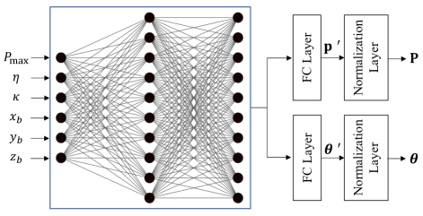
Figure 3: Structure of the proposed PKG-Net in the absence of Eve information.

During the training phase, the PKG-Net learns to update its parameters in an unsupervised manner. The goal is to maximize $I\left(\widetilde{\mathbf{y}}_{a};\widetilde{\mathbf{y}}_{b}^{T}\right)$, namely, minimize the following loss function:

$$\mathcal{L}_{\mathrm{loss}}^{1}=-\frac{1}{K}\sum_{k=1}^{K}I\left(\widetilde{\mathbf{y}}_{a,k};\widetilde{\mathbf{y}}_{b,k}^{T}\right),$$ (55)

where $K$ is the number of training samples, and $\widetilde{\mathbf{y}}_{a,k}$ and $\widetilde{\mathbf{y}}_{b,k}^{T}$ are the channel estimations in the $k$-th training. It is clear that the smaller the loss function, the higher the average SKR. Recall that $\widetilde{\mathbf{y}}_{a}$ and $\widetilde{\mathbf{y}}_{b}^{T}$ are functions of $\mathbf{P}$ and $\mathbf{\theta}$, which are the outputs of PKG-Net. During the training, PKG-Net learns to obtain the optimal $\mathbf{P}$ and $\mathbf{\theta}$ that minimizes the loss function. The training phase is performed offline, and thus the computational complexity is less of a concern.

VI-B Case 2: The Channel Statistics of Eve is Known

In the presence of Eve’s channel statistics, the structure of the proposed PKG-Net is shown in Fig. 4. Besides the location of Bob, transmit power and channel statistics, we also treat the location information of Eve, i.e., $\left(x_{e},y_{e},z_{e}\right)$, as input. The hidden layers and output layer have the same structure as the network presented in the previous subsection. During the training phase, the goal is to maximize $R_{\mathrm{sk}}\left(\widetilde{\mathbf{y}}_{a},\widetilde{\mathbf{y}}_{b},\widetilde{\mathbf{y}}_{e}\right)$, namely, minimize the following loss function:

$$\mathcal{L}_{\mathrm{loss}}^{2}=-\frac{1}{K}\sum_{k=1}^{K}R_{\mathrm{sk}}\left(\widetilde{\mathbf{y}}_{a,k},\widetilde{\mathbf{y}}_{b,k},\widetilde{\mathbf{y}}_{e,k}\right).$$ (56)

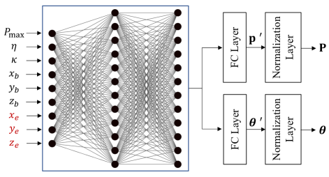
Figure 4: Structure of the proposed PKG-Net with Eve information.

In both cases, during the online inference phase, the BS directly designs the precoding matrix and the IRS phase shifts according to the output of the trained neural network as soon as it gets the input information.

VII Simulation Results

In this section, we numerically evaluate the SKR performance of the proposed PKG-Net in comparison with the benchmark methods.

VII-A Simulation Setup

The coordinates of the BS and the IRS in meters are set as (5, -30, 0) and (0, 0, 0), respectively. The large-scale path loss in dB is computed by

$$\beta_{i}=\beta_{0,i}-10\alpha_{i}\text{log}_{10}\left(d/d_{0}\right),$$ (57)

where $\beta_{0,i}$ is the path loss at the reference distance, $d_{0}=1$ m is the reference distance, $d$ is the transmission distance, and $\alpha_{i}$ is the path-loss exponent. For the direct link, i.e., $i=\mathrm{h}$, we set $\beta_{0,i}=-32.6$ dB and $\alpha_{i}=3.67$; for the reflecting links, i.e., $i=\mathrm{G}$ or $\mathrm{f}$, we set $\beta_{0,i}=-30$ dB and $\alpha_{i}=2.2$. The channel bandwidth is set to $W=20$ MHz and the noise power is computed by $\delta^{2}=-174\ \mathrm{dBm/Hz}+10\mathrm{log}10(W)+10\ \mathrm{dB}$ [35, 28]. The IRS is assumed to be a uniform square array, i.e., $L_{\mathrm{H}}=L_{\mathrm{V}}$. Unless otherwise specified, the transmit power of Bob is set to $P_{b}=10$ dBm, the default spatial correlation coefficient at the BS is set to $\eta=0.4$ and the IRS element spacing is half a wavelength, i.e., $\Delta=\frac{\lambda}{2}$.

During the training of the proposed PKG-Net in both cases, the UE location is uniformly distributed in the $xy$-plane with $x\in[5,15]$ and $y\in[5,15]$ to achieve generalization ability to various UE locations. Moreover, $P_{\mathrm{max}}$ is uniformly distributed in $[10,30]$ dBm, $\eta$ is uniformly distributed in $[0,1]$, and $\kappa$ is uniformly distributed in $[0,10]$. In particular, in case 2, the location of Eve is uniformly distributed in the $xy$-plane with $x\in[5,15]$ and $y\in[5,15]$. In both cases, each hidden layer of the PKG-Net has 100 neurons. In each training epoch, 1000 random UE locations are used as training samples with a batch size of 100. The DNN is implemented using TensorFlow and updated by Adam optimizer with a learning rate of 0.001. The training is terminated when the loss function on the verification data set does not decrease by more than 10 consecutive epochs or the number of training epochs reaches 100.

The proposed algorithms and benchmark methods are summarized as follows:

• PKG-Net w/o Eve info: Represent the PKG-Net in the absence of Eve’s channel statistics proposed in Section VI.

• PKG-Net w/ Eve info: Represent the PKG-Net with Eve information proposed in Section VI.

• Baseline solution w/o Eve info: Represent the water-filling algorithm-based solution proposed in Section V-A.

• Baseline solution w/ Eve info: Represent the water-filling algorithm-based solution proposed in Section V-B.

• Random configuration: Represent a non-optimized scheme, where both the precoding matrix $\mathbf{P}$ and the IRS phase shift vector $\bm{\theta}$ are randomly configured.

VII-B Results

In the following numerical evaluation, the UE location is set to $\left(x_{b},y_{b},z_{b}\right)=(10,10,0)$ and the Eve location is set to $\left(x_{e},y_{e},z_{e}\right)=(x_{b}-0.5\lambda,y_{b},z_{b})$ unless otherwise stated.

In Fig. 5, we show the effect of the number of antennas on the SKR. First, it is observed that the SKR increases linearly with the number of antennas, as more antennas introduce more sub-channels to extract secure keys. Second, we can see that regardless of the number of antennas, the proposed PKG-Net achieves a higher SKR than the two benchmark methods, demonstrating the effectiveness of the proposed DNN-based algorithm. The gap in terms of SKR between the proposed PKG-Net and other benchmark methods increases with the number of antennas, indicating that using more antennas requires a more sophisticated design of BS precoding.

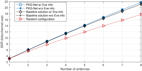
Figure 5: SKR versus $M$ with $P_{\mathrm{max}}=25$ dBm, $\kappa=1$ and $L=36$.

Fig. 6 illustrates the effect of the number of IRS elements on the SKR. As can be observed, the SKR monotonically increases with the number of IRS elements, since more IRS elements provide more reflection links that improve the received signals during channel probings. It is noticed that the SKR gain of increasing IRS elements is not as significant as that of increasing BS antennas. This is because in the proposed PKG system, the downlink pilot length is proportional to the number of antennas. It is expected to achieve a higher SKR when the entire cascaded channel is estimated with a minimum pilot length of $M(L+1)$, which requires a new design of IRS phase shifting and will be of interest in our future work.

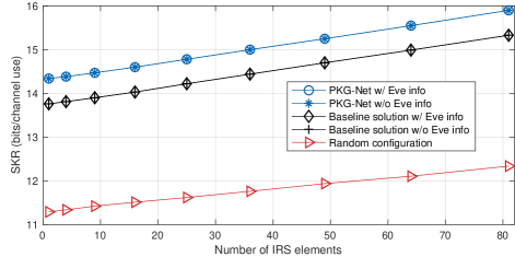
Figure 6: SKR versus $L$ with $P_{\mathrm{max}}=20$ dBm, $\kappa=0$ and $M=6$.

In Fig. 7, the SKR versus the transmit power is displayed. It is shown that the SKR monotonically increases with the transmit power for all the considered optimization methods, which is straightforward due to the fact that a higher transmit power leads to a higher SNR, thereby improving the reciprocity of channel observations at Alice and Bob.

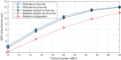
Figure 7: SKR versus $P$ with $\kappa=1$, $M=4$ and $L=36$.

Fig. 8 shows the SKR versus the spatial correlation coefficient at the BS for different UE locations. We can see that the SKR monotonically decreases with the correlation coefficient, which illustrates that the existence of spatial correlation degrades the performance of PKG in terms of SKR. In comparison with the benchmark methods, the proposed PKG-Net can effectively design the BS precoding and IRS phase shifting under different spatial correlation conditions. Interestingly, when the correlation coefficient increases, the SKR gain of the proposed PKG-Net becomes more significant compared to the baseline solution. Furthermore, the proposed PKG-Net shows good generalization to UE locations.

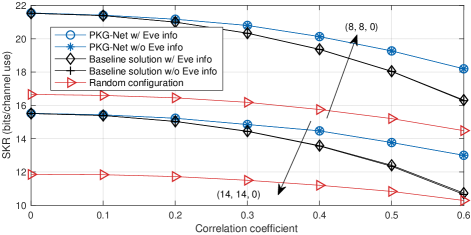
Figure 8: SKR versus $\eta$ with $P_{\mathrm{max}}=20$ dBm, $\kappa=1$, $M=8$ and $L=36$.

In Fig. 9, we present the effect of the distance between Bob and Eve on the SKR. We can observe that the SKR is inversely proportional to the absolute value of channel correlation coefficient between Bob and Eve. It is worth noting that a satisfactory SKR can be achieved when the distance between Bob and Eve is more than about 0.3 wavelength. As stated in [4], Bob can easily find Eve if Eve is within half a wavelength of Bob. Hence, the IRS-assisted multi-antenna system can achieve a good PKG performance.

It is interesting to observe that under various system parameters, almost the same SKR can be achieved regardless of whether Eve information is available, indicating that the optimization objectives in case 1 and case 2 have the same solution. Therefore, in practical implementation, we can obtain a satisfactory SKR using only Bob’s channel statistics.

In practice, the conventional optimization algorithms are more suited to run on a classic central processing unit (CPU) architecture, while the matrix multiplication of the DNNs can be efficiently accelerated by a graphics processing unit (GPU). As such, it is difficult to make a fair comparison with regard to computational time for different algorithms. However, it is still revealing to show the huge difference in computational time between PKG-Net and the baseline solution using the same hardware configuration [36]. In Table I, we present the average computational time of 100 samples for case 1, the UE locations of which are uniformly distributed in the $xy$-plane with $x\in[5,15]$ and $y\in[5,15]$. Other system parameters are set to $P_{\mathrm{max}}=25$ dBm, $\kappa=1$ and $L=36$. Both algorithms run on the same platform, a 4 core Intel Core i7 CPU with 2.2 GHz base frequency and 16GB memory. From Table I, it is clear that PKG-Net has a significantly lower computational time than the baseline solution.

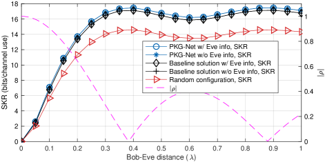
Figure 9: SKR and $|\rho|$ versus the distance between Bob and Eve with $P_{\mathrm{max}}=25$ dBm, $\kappa=1$, $M=6$ and $L=36$.

TABLE I: Comparison of Running Time for Different Schemes

Algorithm	M=2	M=4	M=8
Baseline solution	74.86 ms	106 ms	163 ms
PKG-Net	0.46 ms	0.91 ms	2.48 ms

VIII Conclusions

In this paper, we have studied the PKG in an IRS-assisted multi-antenna system. We have developed a new PKG framework and derived the closed-form expression of SKR considering correlated eavesdropping channels. To maximize the SKR, we proposed a novel DNN-based algorithm, PKG-Net, to jointly configure the precoding matrix at the BS and the phase shift vector at the IRS. The proposed PKG-Net has a good generalization ability to different transmit powers and channel statics. Simulation results show that under various system parameters, the proposed PKG-Net achieves a higher SKR than the benchmark methods. Compared with the baseline solution, PKG-Net has significantly lower computational complexity and can satisfy real-time processing constraints. Additionally, it is observed that the spatial correlation among BS antennas degrades the PKG performance in terms of SKR, and that the proposed PKG-Net can address the spatial correlation more effectively than other benchmark methods. In our future work, we will extend the proposed PKG system to a multi-user scenario and solve the multi-user precoding problem.

Appendix A Proof of Theorem 1

In (III), we further define $R_{\mathrm{sk}}^{1}=I\left(\widetilde{\mathbf{y}}_{a};\widetilde{\mathbf{y}}_{b}^{T}\right)-I\left(\widetilde{\mathbf{y}}_{a};\widetilde{\mathbf{y}}_{e}^{T}\right)$ and $R_{\mathrm{sk}}^{2}=I\left(\widetilde{\mathbf{y}}_{a};\widetilde{\mathbf{y}}_{b}^{T}\right)-I\left(\widetilde{\mathbf{y}}_{b};\widetilde{\mathbf{y}}_{e}^{T}\right)$. Following [33], we have

$$I\left(\widetilde{\mathbf{y}}_{a};\widetilde{\mathbf{y}}_{b}^{T}\right) =H\left(\widetilde{\mathbf{y}}_{a}\right)+H\left(\widetilde{\mathbf{y}}_{b}^{T}\right)-H\left(\widetilde{\mathbf{y}}_{a},\widetilde{\mathbf{y}}_{b}^{T}\right)$$

$$=\log_{2}\left(\frac{|\mathbf{R}_{a}||\mathbf{R}_{b}|}{\left|\bm{\mathcal{R}}_{a,b}\right|}\right),$$ (58)

where

$$\mathbf{R}_{a} =\mathbb{E}\left\{\widetilde{\mathbf{y}}_{a}\widetilde{\mathbf{y}}_{a}^{H}\right\}=P_{b}\left(\widetilde{\bm{\theta}}\otimes\mathbf{P}\right)^{T}\mathbf{R}_{\mathrm{c}}^{\mathrm{U}}\left(\widetilde{\bm{\theta}}\otimes\mathbf{P}\right)^{*}\!+\!\delta^{2}\mathbf{P}^{T}\mathbf{P}^{*},$$ (59)

$$\mathbf{R}_{b} =\mathbb{E}\left\{\widetilde{\mathbf{y}}_{b}^{T}\widetilde{\mathbf{y}}_{b}^{*}\right\}=\left(\widetilde{\bm{\theta}}\otimes\mathbf{P}\right)^{T}\mathbf{R}_{\mathrm{c}}^{\mathrm{U}}\left(\widetilde{\bm{\theta}}\otimes\mathbf{P}\right)^{*}+\delta^{2}\mathbf{I}_{M},$$ (60)

and

$$\bm{\mathcal{R}}_{a,b}=\begin{bmatrix}\mathbf{R}_{a}&\mathbf{R}_{a,b}\\ \mathbf{R}_{b,a}&\mathbf{R}_{b}\end{bmatrix},$$ (61)

with

$$\mathbf{R}_{\mathrm{c}}^{\mathrm{U}} =\mathbb{E}\left\{\mathbf{h}_{\mathrm{c}}^{ab}\left(\mathbf{h}_{\mathrm{c}}^{ab}\right)^{H}\right\}$$

$$=\begin{bmatrix}\beta_{\mathrm{h}_{ab}}\mathbf{R}_{\mathrm{B}}&\mathbf{0}^{T}\\ \mathbf{0}&\frac{\beta_{\mathrm{G}}\beta_{\mathrm{f}_{b}}}{\left({1+\kappa}\right)\left({1+\kappa}\right)}\mathbf{R}_{\mathrm{I}}\odot\mathbf{R}_{\mathrm{I}}\otimes\mathbf{R}_{\mathrm{B}}\end{bmatrix},$$ (62)

$$\mathbf{R}_{a,b} =\mathbf{R}_{b,a}=\mathbb{E}\left\{\widetilde{\mathbf{y}}_{a}\widetilde{\mathbf{y}}_{b}^{*}\right\}=\sqrt{P_{b}}\left(\widetilde{\bm{\theta}}\otimes\mathbf{P}\right)^{T}\mathbf{R}_{\mathrm{c}}^{\mathrm{U}}\left(\widetilde{\bm{\theta}}\otimes\mathbf{P}\right)^{*}.$$ (63)

Following the similar steps, we have

$$I\left(\widetilde{\mathbf{y}}_{a};\widetilde{\mathbf{y}}_{e}^{T}\right)=\log_{2}\left(\frac{|\mathbf{R}_{a}||\mathbf{R}_{e}|}{\left|\bm{\mathcal{R}}_{a,e}\right|}\right),$$ (64)

where

$$\mathbf{R}_{e} =\mathbb{E}\left\{\widetilde{\mathbf{y}}_{e}^{T}\widetilde{\mathbf{y}}_{e}^{*}\right\}=\left(\widetilde{\bm{\theta}}\otimes\mathbf{P}\right)^{T}\mathbf{R}_{\mathrm{c}}^{\mathrm{E}}\left(\widetilde{\bm{\theta}}\otimes\mathbf{P}\right)^{*}+\delta^{2}\mathbf{I}_{M},$$ (65)

and

$$\bm{\mathcal{R}}_{a,e}=\begin{bmatrix}\mathbf{R}_{a}&\mathbf{R}_{a,e}\\ \mathbf{R}_{e,a}&\mathbf{R}_{e}\end{bmatrix},$$ (66)

with

$$\mathbf{R}_{\mathrm{c}}^{\mathrm{E}} =\mathbb{E}\left\{\mathbf{h}_{\mathrm{c}}^{ae}\left(\mathbf{h}_{\mathrm{c}}^{ae}\right)^{H}\right\}$$

$$=\begin{bmatrix}\beta_{\mathrm{h}_{ae}}\mathbf{R}_{\mathrm{B}}&\mathbf{0}^{T}\\ \mathbf{0}&\frac{\beta_{\mathrm{G}}\beta_{\mathrm{f}_{e}}}{\left({1+\kappa}\right)\left({1+\kappa}\right)}\mathbf{R}_{\mathrm{I}}\odot\mathbf{R}_{\mathrm{I}}\otimes\mathbf{R}_{\mathrm{B}}\end{bmatrix},$$ (67)

$$\mathbf{R}_{a,e} =\mathbf{R}_{e,a}=\mathbb{E}\left\{\widetilde{\mathbf{y}}_{a}\widetilde{\mathbf{y}}_{e}^{*}\right\}=\sqrt{P_{b}}\left(\widetilde{\bm{\theta}}\otimes\mathbf{P}\right)^{T}\mathbf{R}_{\mathrm{c}}^{\mathrm{U,E}}\left(\widetilde{\bm{\theta}}\otimes\mathbf{P}\right)^{*},$$ (68)

where

$${\mathbf{R}_{\mathrm{c}}^{\mathrm{U,E}}}\!=\!\mathbb{E}\left\{\mathbf{h}_{\mathrm{c}}^{ab}\left(\mathbf{h}_{\mathrm{c}}^{ae}\right)^{H}\right\}=$$

$$\begin{bmatrix}\rho\beta_{\mathrm{h}_{ab}}\beta_{\mathrm{h}_{ae}}\mathbf{R}_{\mathrm{B}}\!&\!\!\mathbf{0}^{T}\!\\ \mathbf{0}\!&\!\!\frac{\rho\beta_{\mathrm{G}}}{1+\kappa}\sqrt{\frac{\beta_{\mathrm{f}_{b}}\beta_{\mathrm{f}_{e}}}{({1+\kappa})({1+\kappa})}}\mathbf{R}_{\mathrm{I}}\!\odot\!\mathbf{R}_{\mathrm{I}}\!\otimes\!\mathbf{R}_{\mathrm{B}}\!\end{bmatrix}\!.\!$$ (69)

Moreover,

$$I\left(\widetilde{\mathbf{y}}_{b};\widetilde{\mathbf{y}}_{e}^{T}\right)=\log_{2}\left(\frac{|\mathbf{R}_{b}||\mathbf{R}_{e}|}{\left|\bm{\mathcal{R}}_{b,e}\right|}\right),$$ (70)

where

$$\bm{\mathcal{R}}_{b,e}=\begin{bmatrix}\mathbf{R}_{b}&\mathbf{R}_{b,e}\\ \mathbf{R}_{e,b}&\mathbf{R}_{e}\end{bmatrix},$$ (71)

with

$$\mathbf{R}_{b,e}\!=\!\mathbf{R}_{e,b}\!=\!\mathbb{E}\left\{\widetilde{\mathbf{y}}_{b}\widetilde{\mathbf{y}}_{e}^{*}\right\}\!=\!\left(\widetilde{\bm{\theta}}\otimes\mathbf{P}\right)^{T}\mathbf{R}_{\mathrm{c}}^{\mathrm{U,E}}\left(\widetilde{\bm{\theta}}\otimes\mathbf{P}\right)^{*}.$$ (72)

Then we have

$$R_{\mathrm{sk}}^{1}=I\left(\widetilde{\mathbf{y}}_{a};\widetilde{\mathbf{y}}_{b}^{T}\right)-I\left(\widetilde{\mathbf{y}}_{a};\widetilde{\mathbf{y}}_{e}^{T}\right)=\log_{2}\left(\frac{|\mathbf{R}_{b}|\left|\bm{\mathcal{R}}_{a,e}\right|}{|\mathbf{R}_{e}|\left|\bm{\mathcal{R}}_{a,b}\right|}\right),$$ (73)

$$R_{\mathrm{sk}}^{2}=I\left(\widetilde{\mathbf{y}}_{a};\widetilde{\mathbf{y}}_{b}^{T}\right)-I\left(\widetilde{\mathbf{y}}_{b};\widetilde{\mathbf{y}}_{e}^{T}\right)=\log_{2}\left(\frac{|\mathbf{R}_{a}|\left|\bm{\mathcal{R}}_{b,e}\right|}{|\mathbf{R}_{e}|\left|\bm{\mathcal{R}}_{a,b}\right|}\right).$$ (74)

Define that $\mathbf{R}_{\mathrm{Z}}^{\mathrm{U}}=\left(\widetilde{\bm{\theta}}\otimes\mathbf{P}\right)^{T}\mathbf{R}_{\mathrm{c}}^{\mathrm{U}}\left(\widetilde{\bm{\theta}}\otimes\mathbf{P}\right)^{*}$, $\mathbf{R}_{\mathrm{Z}}^{\mathrm{E}}=\left(\widetilde{\bm{\theta}}\otimes\mathbf{P}\right)^{T}\mathbf{R}_{\mathrm{c}}^{\mathrm{E}}\left(\widetilde{\bm{\theta}}\otimes\mathbf{P}\right)^{*}$ and $\mathbf{R}_{\mathrm{Z}}^{\mathrm{U},\mathrm{E}}=\left(\widetilde{\bm{\theta}}\!\otimes\!\mathbf{P}\right)^{T}\mathbf{R}_{\mathrm{c}}^{\mathrm{U},\mathrm{E}}\left(\widetilde{\bm{\theta}}\!\otimes\!\mathbf{P}\right)^{*}$. (33) can be obtained by plugging (60), (63), (65) and (66) into (73), and (34) can be obtained by plugging (59), (63), (65) and (72) into (74). This completes the proof.

Appendix B Proof of Lemma 1

Plugging (21) and (23) into (A), we have

$$\mathbf{R}_{a}$$

$$\!=\!P_{b}\mathbf{P}^{T\!}\mathbb{E}\!\left\{\!\left(\mathbf{h}_{ab}^{\mathrm{NL}}\!+\!\mathbf{G}^{\mathrm{\!NL\!}}\mathbf{\Theta}\mathbf{f}_{b}^{\mathrm{NL}}\right)\left(\left(\mathbf{h}_{ab}^{\mathrm{NL}}\right)^{\!H\!}\!+\!\left(\mathbf{G}^{\mathrm{\!NL\!}}\mathbf{\Theta}\mathbf{f}_{b}^{\mathrm{NL}}\right)^{\!H\!}\right)\!\right\}\!\mathbf{P}^{*\!}$$

$$~{}~{}~{}~{}~{}~{}~{}~{}~{}~{}~{}~{}~{}~{}~{}~{}~{}~{}~{}~{}~{}~{}~{}~{}~{}~{}~{}~{}~{}~{}~{}~{}~{}~{}~{}~{}~{}~{}~{}~{}~{}~{}~{}~{}~{}~{}~{}~{}~{}~{}~{}~{}~{}~{}~{}~{}~{}+\delta^{2}\mathbf{P}^{T}\mathbf{P}^{*},$$

$$\!=\!P_{b}\mathbf{P}^{T}\Big{(}\mathbb{E}\left\{\left(\mathbf{h}_{ab}^{\mathrm{NL}}\left(\mathbf{h}_{ab}^{\mathrm{NL}}\right)^{\!H\!}\right)\right\}$$

$$~{}~{}~{}+\mathbb{E}\left\{\left(\mathbf{G}^{\mathrm{\!NL\!}}\mathbf{\Theta}\mathbf{f}_{b}^{\mathrm{NL}}\right)\left(\mathbf{G}^{\mathrm{\!NL\!}}\mathbf{\Theta}\mathbf{f}_{b}^{\mathrm{NL}}\right)^{\!H\!}\right\}\Big{)}\mathbf{P}^{*\!}+\delta^{2}\mathbf{P}^{T}\mathbf{P}^{*},$$

$$\!=\!P_{b}\mathbf{P}^{T}\Big{(}\beta_{\mathrm{h}_{ab}}\mathbf{R}_{\mathrm{B}}$$

$$~{}~{}~{}+\mathbb{E}\left\{\left(\mathbf{G}^{\mathrm{\!NL\!}}\mathbf{\Theta}\mathbf{f}_{b}^{\mathrm{NL}}\right)\left(\mathbf{G}^{\mathrm{\!NL\!}}\mathbf{\Theta}\mathbf{f}_{b}^{\mathrm{NL}}\right)^{\!H\!}\right\}\Big{)}\mathbf{P}^{*\!}+\delta^{2}\mathbf{P}^{T}\mathbf{P}^{*},$$ (75)

where

$$\mathbb{E}\left\{\left(\mathbf{G}^{\mathrm{\!NL\!}}\mathbf{\Theta}\mathbf{f}_{b}^{\mathrm{NL}}\right)\left(\mathbf{G}^{\mathrm{\!NL\!}}\mathbf{\Theta}\mathbf{f}_{b}^{\mathrm{NL}}\right)^{\!H\!}\right\}$$

$$=\mathbb{E}\left\{\mathbf{R}_{\mathrm{B}}^{\frac{1}{2}}\widetilde{\mathbf{G}}\mathbf{R}_{\mathrm{I}}^{\frac{1}{2}}\mathbf{\Theta}\mathbf{R}_{\mathrm{I}}^{\frac{1}{2}}\widetilde{\mathbf{f}}_{b}\widetilde{\mathbf{f}}_{b}^{H}\mathbf{R}_{\mathrm{I}}^{\frac{H}{2}}\mathbf{\Theta}^{*}\mathbf{R}_{\mathrm{I}}^{\frac{H}{2}}\widetilde{\mathbf{G}}^{H}\mathbf{R}_{\mathrm{B}}^{\frac{H}{2}}\right\}$$

$$\overset{(a)}{=}\mathbf{R}_{\mathrm{B}}\mathbb{E}\left\{\widetilde{\mathbf{G}}\mathbf{R}_{\mathrm{I}}^{\frac{1}{2}}\mathbf{\Theta}\mathbf{R}_{\mathrm{I}}^{\frac{1}{2}}\widetilde{\mathbf{f}}_{b}\widetilde{\mathbf{f}}_{b}^{H}\mathbf{R}_{\mathrm{I}}^{\frac{H}{2}}\mathbf{\Theta}^{*}\mathbf{R}_{\mathrm{I}}^{\frac{H}{2}}\widetilde{\mathbf{G}}^{H}\right\}$$

$$=\mathbf{R}_{\mathrm{B}}\mathbb{E}\left\{\text{vec}\left(\widetilde{\mathbf{G}}\mathbf{R}_{\mathrm{I}}^{\frac{1}{2}}\mathbf{\Theta}\mathbf{R}_{\mathrm{I}}^{\frac{1}{2}}\widetilde{\mathbf{f}}_{b}\right)\left(\text{vec}\left(\widetilde{\mathbf{G}}\mathbf{R}_{\mathrm{I}}^{\frac{1}{2}}\mathbf{\Theta}\mathbf{R}_{\mathrm{I}}^{\frac{1}{2}}\widetilde{\mathbf{f}}_{b}\right)\right)^{H}\right\}$$

$$=\mathbf{R}_{\mathrm{B}}\mathbb{E}\bigg{\{}\left(\left(\mathbf{R}_{\mathrm{I}}^{\frac{1}{2}}\mathbf{\Theta}\mathbf{R}_{\mathrm{I}}^{\frac{1}{2}}\widetilde{\mathbf{f}}_{b}\right)^{\!T\!}\!\otimes\!\mathbf{I}_{M}\right)\text{vec}\left(\widetilde{\mathbf{G}}\right)\left(\text{vec}\left(\widetilde{\mathbf{G}}\right)\right)^{H}$$

$$~{}~{}~{}~{}~{}~{}~{}~{}~{}~{}~{}~{}~{}~{}~{}~{}~{}~{}~{}~{}~{}~{}~{}~{}~{}~{}~{}~{}~{}~{}~{}~{}~{}~{}~{}~{}~{}~{}\times\left(\left(\mathbf{R}_{\mathrm{I}}^{\frac{1}{2}}\mathbf{\Theta}\mathbf{R}_{\mathrm{I}}^{\frac{1}{2}}\widetilde{\mathbf{f}}_{b}\right)^{\!*\!}\!\otimes\!\mathbf{I}_{M}\right)\bigg{\}}$$

$$=\frac{\beta_{\mathrm{G}}}{1+\kappa}\mathbf{R}_{\mathrm{B}}\mathbb{E}\bigg{\{}\left(\left(\mathbf{R}_{\mathrm{I}}^{\frac{1}{2}}\mathbf{\Theta}\mathbf{R}_{\mathrm{I}}^{\frac{1}{2}}\widetilde{\mathbf{f}}_{b}\right)^{\!T\!}\!\otimes\!\mathbf{I}_{M}\right)$$

$$~{}~{}~{}~{}~{}~{}~{}~{}~{}~{}~{}~{}~{}~{}~{}~{}~{}~{}~{}~{}~{}~{}~{}~{}~{}~{}~{}~{}~{}~{}~{}~{}~{}~{}~{}~{}~{}~{}\times\left(\left(\mathbf{R}_{\mathrm{I}}^{\frac{1}{2}}\mathbf{\Theta}\mathbf{R}_{\mathrm{I}}^{\frac{1}{2}}\widetilde{\mathbf{f}}_{b}\right)^{\!*\!}\!\otimes\!\mathbf{I}_{M}\right)\bigg{\}}$$

$$\overset{(b)}{=}\frac{\beta_{\mathrm{G}}}{1+\kappa}\mathbf{R}_{\mathrm{B}}\mathbb{E}\left\{\left(\mathbf{R}_{\mathrm{I}}^{\frac{1}{2}}\mathbf{\Theta}\mathbf{R}_{\mathrm{I}}^{\frac{1}{2}}\widetilde{\mathbf{f}}_{b}\right)^{\!T\!}\left(\mathbf{R}_{\mathrm{I}}^{\frac{1}{2}}\mathbf{\Theta}\mathbf{R}_{\mathrm{I}}^{\frac{1}{2}}\widetilde{\mathbf{f}}_{b}\right)^{\!*\!}\!\otimes\!\mathbf{I}_{M}\right\}$$

$$=\frac{\beta_{\mathrm{G}}}{1+\kappa}\mathbf{R}_{\mathrm{B}}\mathbb{E}\left\{\left(\text{vec}\left(\mathbf{R}_{\mathrm{I}}^{\frac{1}{2}}\mathbf{\Theta}\mathbf{R}_{\mathrm{I}}^{\frac{1}{2}}\widetilde{\mathbf{f}}_{b}\right)\right)^{\!T\!}\!\left(\!\text{vec}\left(\mathbf{R}_{\mathrm{I}}^{\frac{1}{2}}\mathbf{\Theta}\mathbf{R}_{\mathrm{I}}^{\frac{1}{2}}\widetilde{\mathbf{f}}_{b}\right)\right)^{\!*\!}\right\}$$

$$=\frac{\beta_{\mathrm{G}}}{1+\kappa}\mathbf{R}_{\mathrm{B}}\mathbb{E}\bigg{\{}\left(\text{vec}\left(\mathbf{R}_{\mathrm{I}}^{\frac{1}{2}}\mathbf{\Theta}\mathbf{R}_{\mathrm{I}}^{\frac{1}{2}}\right)\right)^{T}\left(\widetilde{\mathbf{f}}_{b}\otimes\mathbf{I}_{L}\right)$$

$$~{}~{}~{}~{}~{}~{}~{}~{}~{}~{}~{}~{}~{}~{}~{}~{}~{}~{}~{}~{}~{}~{}~{}~{}~{}~{}~{}~{}\times\left(\widetilde{\mathbf{f}}_{b}^{H}\otimes\mathbf{I}_{L}\right)\left(\text{vec}\left(\mathbf{R}_{\mathrm{I}}^{\frac{1}{2}}\mathbf{\Theta}\mathbf{R}_{\mathrm{I}}^{\frac{1}{2}}\right)\right)^{*}\bigg{\}}$$

$$=\frac{\beta_{\mathrm{G}}\beta_{\mathrm{f}_{b}}}{\left({1\!+\!\kappa}\right)\left({1\!+\!\kappa}\right)}\mathbf{R}_{\mathrm{B}}\left(\text{vec}\!\left(\!\mathbf{R}_{\mathrm{I}}^{\frac{1}{2}}\mathbf{\Theta}\mathbf{R}_{\mathrm{I}}^{\frac{1}{2}}\right)\right)^{\!T\!}\!\left(\!\text{vec}\left(\mathbf{R}_{\mathrm{I}}^{\frac{1}{2}}\mathbf{\Theta}\mathbf{R}_{\mathrm{I}}^{\frac{1}{2}}\right)\right)^{\!*\!}$$

$$=\frac{\beta_{\mathrm{G}}\beta_{\mathrm{f}_{b}}}{\left({1\!+\!\kappa}\right)\left({1\!+\!\kappa}\right)}\mathbf{R}_{\mathrm{B}}\bm{\theta}^{H}(\mathbf{R}_{\mathrm{I}}\odot\mathbf{R}_{\mathrm{I}})\bm{\theta},$$ (76)

where (a) comes from the commutative property of diagonal matrices, and (b) is because $(\mathbf{A}\otimes\mathbf{B})(\mathbf{C}\otimes\mathbf{D})=\mathbf{A}\mathbf{C}\otimes\mathbf{B}\mathbf{D}$. $\mathbf{R}_{b}$ and $\bm{\mathcal{R}}_{a,b}$ can be obtained following the similar steps, which concludes the proof.

Appendix C Proof of Corollary 1

$$\widehat{I}\left(\widetilde{\mathbf{y}}_{a};\widetilde{\mathbf{y}}_{b}^{T}\right) =\sum_{i=1}^{M}\log_{2}\left(\frac{(P_{b}P_{a}\delta_{\mathrm{U}}^{2}p_{i}^{2}+\delta^{2}P_{a})\left(P_{a}\delta_{\mathrm{U}}^{2}p_{i}^{2}+\delta^{2}\right)}{\delta^{2}P_{b}P_{a}\delta_{\mathrm{U}}^{2}p_{i}^{2}+\delta^{2}P_{a}^{2}\delta_{\mathrm{U}}^{2}p_{i}^{2}+\delta^{4}P_{a}}\right)$$

$$=\sum_{i=1}^{M}\log_{2}\left(1+\frac{P_{b}P_{a}\delta_{\mathrm{U}}^{4}p_{i}^{4}}{\delta^{2}P_{b}\delta_{\mathrm{U}}^{2}p_{i}^{2}+\delta^{2}P_{a}\delta_{\mathrm{U}}^{2}p_{i}^{2}+\delta^{4}}\right).$$ (77)

To find the monotonicity of $\widehat{I}\left(\widetilde{\mathbf{y}}_{a};\widetilde{\mathbf{y}}_{b}^{T}\right)$ with regard to $\delta_{\mathrm{U}}^{2}$, we define $f_{i}(x)=\frac{P_{b}P_{a}x^{2}p_{i}^{4}}{\delta^{2}P_{b}xp_{i}^{2}+\delta^{2}P_{a}xp_{i}^{2}+\delta^{4}}$. The first derivative of $f_{i}(x)$ is calculated as

$$\frac{\mathrm{d}f_{i}(x)}{\mathrm{d}x}=\frac{P_{a}P_{b}xp_{i}^{4}\left(2\delta^{4}+P_{a}\delta^{2}xp_{i}^{2}+P_{b}\delta^{2}xp_{i}^{2}\right)}{\left(\delta^{4}+P_{a}\delta^{2}xp_{i}^{2}+P_{b}\delta^{2}xp_{i}^{2}\right)^{2}}.$$ (78)

When $x>0$, we have $\frac{\mathrm{d}(f_{i}(x))}{\mathrm{d}x}>0$. Hence, $f_{i}(x)$ monotonically increases with $x$. We then rewrite (C) as

$$\widehat{I}\left(\widetilde{\mathbf{y}}_{a};\widetilde{\mathbf{y}}_{b}^{T}\right)=\sum_{i=1}^{M}\log_{2}\left(1+f_{i}(\delta_{\mathrm{U}}^{2})\right).$$ (79)

From (79), it is clear that $\widehat{I}\left(\widetilde{\mathbf{y}}_{a};\widetilde{\mathbf{y}}_{b}^{T}\right)$ monotonically increases with $\delta_{\mathrm{U}}^{2}$. Recall that

$$\delta_{\mathrm{U}}^{2} =\beta_{\mathrm{h}_{ab}}+\frac{\beta_{\mathrm{G}}\beta_{\mathrm{f}_{b}}}{\left({1+\kappa}\right)\left({1+\kappa}\right)}\bm{\theta}^{H}(\mathbf{R}_{\mathrm{I}}\odot\mathbf{R}_{\mathrm{I}})\bm{\theta}$$

$$=\beta_{\mathrm{h}_{ab}}+\frac{\beta_{\mathrm{G}}\beta_{\mathrm{f}_{b}}}{\left({1+\kappa}\right)\left({1+\kappa}\right)}\Bigg{(}\sum_{l=1}^{L}\left[\mathbf{R}_{\mathrm{I}}\odot\mathbf{R}_{\mathrm{I}}\right]_{l,l}+$$

$$~{}~{}~{}~{}~{}~{}~{}~{}~{}~{}~{}~{}~{}~{}~{}~{}\sum_{i=1}^{L}\sum_{j>i}^{L}2\left[\mathbf{R}_{\mathrm{I}}\odot\mathbf{R}_{\mathrm{I}}\right]_{i,j}\text{cos}\big{(}\theta_{i}-\theta_{j}\big{)}\Bigg{)}.$$ (80)

As such, $\delta_{\mathrm{U}}^{2}$ is maximized when $\theta_{i}=\theta_{j},\forall i\neq j$.

References

• [1] C. Chen, J. Zhang, T. Lu, M. Sandell, and L. Chen, “Machine learning-based secret key generation for IRS-assisted multi-antenna systems,” arXiv preprint arXiv:2301.08179, 2023.
• [2] A. Chorti, A. N. Barreto, S. Köpsell, M. Zoli, M. Chafii, P. Sehier, G. Fettweis, and H. V. Poor, “Context-aware security for 6g wireless: the role of physical layer security,” IEEE Commun. Stand. Mag., vol. 6, no. 1, pp. 102–108, 2022.
• [3] V.-L. Nguyen, P.-C. Lin, B.-C. Cheng, R.-H. Hwang, and Y.-D. Lin, “Security and privacy for 6G: A survey on prospective technologies and challenges,” IEEE Commun. Surv. Tutor., vol. 23, no. 4, pp. 2384–2428, 2021.
• [4] J. Zhang, G. Li, A. Marshall, A. Hu, and L. Hanzo, “A new frontier for iot security emerging from three decades of key generation relying on wireless channels,” IEEE Access, vol. 8, pp. 138 406–138 446, 2020.
• [5] M. Waqas, M. Ahmed, Y. Li, D. Jin, and S. Chen, “Social-aware secret key generation for secure device-to-device communication via trusted and non-trusted relays,” IEEE Trans. Wirel. Commun., vol. 17, no. 6, pp. 3918–3930, 2018.
• [6] S. Bakşi and D. C. Popescu, “Secret key generation with precoding and role reversal in MIMO wireless systems,” IEEE Trans. Wirel. Commun., vol. 18, no. 6, pp. 3104–3112, 2019.
• [7] S. N. Premnath et al., “Secret key extraction from wireless signal strength in real environments,” IEEE Trans. Mobile Comput., vol. 12, no. 5, pp. 917–930, 2013.
• [8] J. Zhang, A. Marshall, and L. Hanzo, “Channel-envelope differencing eliminates secret key correlation: LoRa-based key generation in low power wide area networks,” IEEE Trans. Veh. Technol., vol. 67, no. 12, pp. 12 462–12 466, 2018.
• [9] C. Chen, “Sample-grouping-based vector quantization for secret key extraction from atmospheric optical wireless channels,” IEEE Trans. Wirel. Commun., vol. 21, no. 11, pp. 8905–8918, 2022.
• [10] N. Aldaghri and H. Mahdavifar, “Physical layer secret key generation in static environments,” IEEE Trans. Inf. Forensics Secur., vol. 15, pp. 2692–2705, 2020.
• [11] E. Björnson, H. Wymeersch, B. Matthiesen, P. Popovski, L. Sanguinetti, and E. de Carvalho, “Reconfigurable intelligent surfaces: A signal processing perspective with wireless applications,” IEEE Signal Process. Mag., vol. 39, no. 2, pp. 135–158, 2022.
• [12] Q. Wu, S. Zhang, B. Zheng, C. You, and R. Zhang, “Intelligent reflecting surface-aided wireless communications: A tutorial,” IEEE Trans Commun., vol. 69, no. 5, pp. 3313–3351, 2021.
• [13] T. Lu, L. Chen, J. Zhang, K. Cao, and A. Hu, “Reconfigurable intelligent surface assisted secret key generation in quasi-static environments,” IEEE Commun. Lett., vol. 26, no. 2, pp. 244–248, Feb. 2022.
• [14] P. Staat, H. Elders-Boll, M. Heinrichs, R. Kronberger, C. Zenger, and C. Paar, “Intelligent reflecting surface-assisted wireless key generation for low-entropy environments,” in Proc. IEEE 32nd Annual Int. Symp. on Personal, Indoor and Mobile Radio Commun. (PIMRC), 2021, pp. 745–751.
• [15] Z. Ji, P. L. Yeoh, D. Zhang, G. Chen, Z. He, H. Yin, and Y. li, “Secret key generation for intelligent reflecting surface assisted wireless communication networks,” IEEE Trans. Veh. Technol., vol. 70, no. 1, pp. 1030–1034, Jan. 2021.
• [16] G. Li, C. Sun, W. Xu, M. D. Renzo, and A. Hu, “On maximizing the sum secret key rate for reconfigurable intelligent surface-assisted multiuser systems,” IEEE Trans. Inf. Forensics Security, vol. 17, pp. 211–225, Jan. 2022.
• [17] J. Zhang, E. Björnson, M. Matthaiou, D. W. K. Ng, H. Yang, and D. J. Love, “Prospective multiple antenna technologies for beyond 5G,” IEEE J. Sel. Areas Commun., vol. 38, no. 8, pp. 1637–1660, 2020.
• [18] C. Chen, J. Zhang, X. Chu, and J. Zhang, “On the deployment of small cells in 3D HetNets with multi-antenna base stations,” IEEE Trans. Wirel. Commun., vol. 21, no. 11, pp. 9761–9774, 2022.
• [19] L. Hu, G. Li, X. Qian, A. Hu, and D. W. K. Ng, “Reconfigurable intelligent surface-assisted secret key generation in spatially correlated channels,” arXiv preprint arXiv:2211.03132, 2022.
• [20] T. Lu, L. Chen, J. Zhang, C. Chen, and A. Hu, “Joint precoding and phase shift design in reconfigurable intelligent surfaces-assisted secret key generation,” IEEE Trans. Inf. Forensics Secur., early access, Apr. 20, 2023, doi: 10.1109/TIFS.2023.3268881.
• [21] J. Wang, C. Jiang, H. Zhang, Y. Ren, K.-C. Chen, and L. Hanzo, “Thirty years of machine learning: The road to pareto-optimal wireless networks,” IEEE Commun. Surv. Tutor., vol. 22, no. 3, pp. 1472–1514, 2020.
• [22] N. Kato, B. Mao, F. Tang, Y. Kawamoto, and J. Liu, “Ten challenges in advancing machine learning technologies toward 6G,” IEEE Wireless Commun., vol. 27, no. 3, pp. 96–103, 2020.
• [23] A. Taha, M. Alrabeiah, and A. Alkhateeb, “Enabling large intelligent surfaces with compressive sensing and deep learning,” IEEE Access, vol. 9, pp. 44 304–44 321, 2021.
• [24] C. Huang, R. Mo, and C. Yuen, “Reconfigurable intelligent surface assisted multiuser MISO systems exploiting deep reinforcement learning,” IEEE J. Sel. Areas Commun., vol. 38, no. 8, pp. 1839–1850, 2020.
• [25] S. Zhang, S. Zhang, F. Gao, J. Ma, and O. A. Dobre, “Deep learning optimized sparse antenna activation for reconfigurable intelligent surface assisted communication,” IEEE Trans. Commun., vol. 69, no. 10, pp. 6691–6705, 2021.
• [26] C. Chen, S. Xu, J. Zhang, and J. Zhang, “A distributed machine learning-based approach for IRS-enhanced cell-free MIMO networks,” arXiv preprint arXiv:2301.08077, 2023.
• [27] L. Jiao, G. Sun, J. Le, and K. Zeng, “Machine learning-assisted wireless phy key generation with reconfigurable intelligent surfaces,” in Proc. of the 3rd ACM Workshop on Wireless Security and Mach. Learning, 2021, pp. 61–66.
• [28] E. Björnson and L. Sanguinetti, “Rayleigh fading modeling and channel hardening for reconfigurable intelligent surfaces,” IEEE Wireless Commun. Lett., vol. 10, no. 4, pp. 830–834, Apr. 2020.
• [29] Q. Zhu and Y. Hua, “Optimal pilots for maximal capacity of secret key generation,” in Proc. IEEE GLOBECOM 2019, Hawaii, USA, Dec. 2019, pp. 0–5.
• [30] J. W. Wallace and R. K. Sharma, “Automatic secret keys from reciprocal MIMO wireless channels: Measurement and analysis,” IEEE Trans. Inf. Forensics Security, vol. 5, no. 3, pp. 381–392, 2010.
• [31] U. Maurer, “Secret key agreement by public discussion from common information,” IEEE Trans. Inf. Theory., vol. 39, no. 3, pp. 733–742, 1993.
• [32] J. Zhang, B. He, T. Q. Duong, and R. Woods, “On the key generation from correlated wireless channels,” IEEE Commun. Lett., vol. 21, no. 4, pp. 961–964, 2017.
• [33] B. T. Quist and M. A. Jensen, “Maximization of the channel-based key establishment rate in MIMO systems,” IEEE Trans. Wirel. Commun., vol. 14, no. 10, pp. 5565–5573, 2015.
• [34] C. Xing, Y. Jing, S. Wang, S. Ma, and H. V. Poor, “New viewpoint and algorithms for water-filling solutions in wireless communications,” IEEE Trans. Signal Process., vol. 68, pp. 1618–1634, Feb. 2020.
• [35] S. Buzzi, C. D’Andrea, A. Zappone, M. Fresia, Y.-P. Zhang, and S. Feng, “RIS configuration, beamformer design, and power control in single-cell and multi-cell wireless networks,” IEEE Trans. Cogn. Commun. Netw., vol. 7, no. 2, pp. 398–411, 2021.
• [36] M. Zaher, Ö. T. Demir, E. Björnson, and M. Petrova, “Learning-based downlink power allocation in cell-free massive MIMO systems,” IEEE Trans. Wirel. Commun., vol. 22, no. 1, pp. 174–188, 2022.