ViP-NeRF: Visibility Prior for Sparse Input Neural Radiance Fields

Abstract.

Neural radiance fields (NeRF) have achieved impressive performances in view synthesis by encoding neural representations of a scene. However, NeRFs require hundreds of images per scene to synthesize photo-realistic novel views. Training them on sparse input views leads to overfitting and incorrect scene depth estimation resulting in artifacts in the rendered novel views. Sparse input NeRFs were recently regularized by providing dense depth estimated from pre-trained networks as supervision, to achieve improved performance over sparse depth constraints. However, we find that such depth priors may be inaccurate due to generalization issues. Instead, we hypothesize that the visibility of pixels in different input views can be more reliably estimated to provide dense supervision. In this regard, we compute a visibility prior through the use of plane sweep volumes, which does not require any pre-training. By regularizing the NeRF training with the visibility prior, we successfully train the NeRF with few input views. We reformulate the NeRF to also directly output the visibility of a 3D point from a given viewpoint to reduce the training time with the visibility constraint. On multiple datasets, our model outperforms the competing sparse input NeRF models including those that use learned priors. The source code for our model can be found on our project page: https://nagabhushansn95.github.io/publications/2023/ViP-NeRF.html.

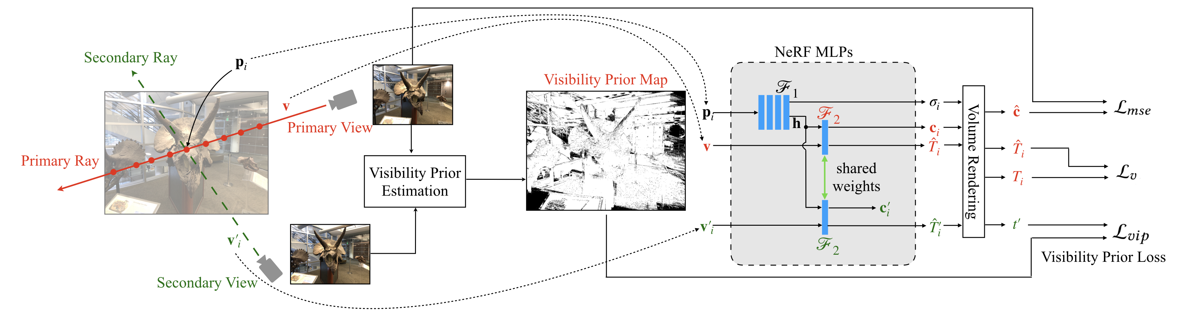
Figure 1. Overview of ViP-NeRF architecture. Given the images from primary and secondary views, we estimate a visibility prior map in the primary view and use it to supervise the visibility of pixels as predicted by the NeRF. Specifically, we cast a ray through a randomly selected pixel in the primary view and sample 3D points along the ray. For every point $\mathbf{p}_{i}$, we use the NeRF MLPs to obtain its visibility in primary and secondary views, along with volume density $\sigma_{i}$ and color $\mathbf{c}_{i}$. Volume rendering outputs visibility $t^{\prime}$ of the chosen pixel in the secondary view which is supervised by the visibility prior. $\mathcal{L}_{v}$ constrains the visibilities $\hat{T}_{i}$ output by network and $T_{i}$ computed using volume rendering to be consistent with each other.

1. Introduction

The goal of novel view synthesis is to synthesize a scene from novel viewpoints given RGB images of a few other viewpoints and their relative camera poses. By representing the scene implicitly using multi-layer perceptrons (MLP) and employing volume rendering, neural radiance fields (NeRF) (Mildenhall et al., 2020; Barron et al., 2021, 2022; Liu et al., 2022) have achieved impressive view synthesis performance. Such superior performance is usually achieved when a large number of views is input to train the NeRF. However, in multiple applications such as virtual or augmented reality, telepresence, robotics, and autonomous driving, very few input images may be available for training (Niemeyer et al., 2022). In such settings, external sensors or a pre-calibrated fixed camera array may be employed to obtain accurate camera poses. Thus, there is a need to train NeRFs with few input views referred to as the sparse input NeRF problem.

The key challenge with sparse input images is that the volume rendering equations in NeRF are under-constrained, leading to solutions that overfit the input views. This results in uncertain and inaccurate depth in the learned representation. Synthesized novel views in such cases contain extreme distortions such as blur, ghosting, and floater artifacts (Niemeyer et al., 2022; Roessle et al., 2022). Recent works have proposed different approaches to constrain the training of NeRF to output visually pleasing novel views. While a few recent works (Zhang et al., 2021; Yang et al., 2022; Zhou and Tulsiani, 2022) focus on training NeRF models on a specific category of objects such as chairs or airplanes, we focus on training category agnostic sparse input NeRF models (Niemeyer et al., 2022). Such prior work can be broadly classified into conditional NeRF models and other regularization approaches.

The conditional NeRF models employ a latent representation of the scene obtained by pre-training on a large dataset of different scenes (Yu et al., 2021; Chen et al., 2021; Wang et al., 2021; Hamdi et al., 2022; Johari et al., 2022) to condition the NeRF. The latent prior helps overcome the limitation on the number of views by enabling the NeRF model to effectively understand the scene. Such an approach is popular even when only a single image of the scene is available as input to the NeRF (Xu et al., 2022; Lin et al., 2023; Cai et al., 2022). Different from the above, MetaNeRF (Tancik et al., 2021) learns the latent information as initial weights of the NeRF MLPs by employing meta-learning. However, the pre-trained latent prior could suffer from poor generalization on a given target scene (Niemeyer et al., 2022). Thus, we believe that there is a need to study the sparse-input NeRF without conditioning the NeRF on latent representations.

On the other hand, regularization based approaches constrain the NeRF training with novel loss functions to yield better solutions. DS-NeRF (Deng et al., 2022) uses sparse depth provided by a structure from motion (SfM) model as additional supervision for the NeRF. To provide richer dense supervision, DDP-NeRF (Roessle et al., 2022) completes the sparse depth map using a pre-trained convolutional neural network (CNN). However, the requirement of pre-training on a large dataset of scenes is cumbersome and the dense depth prior may suffer from generalization errors. RegNeRF (Niemeyer et al., 2022) and InfoNeRF (Kim et al., 2022) impose constraints to promote depth smoothness and reduce depth uncertainty respectively. However, in our experiments, we observe that these methods are still inferior to DS-NeRF on popular datasets. This motivates the exploration of other reliable features for dense supervision to constrain the NeRF in addition to sparse depth supervision.

In our work, we explore the use of regularization in terms of visibility of any pixel from a pair of viewpoints. Here visibility of a pixel refers to whether the corresponding object is seen in both the viewpoints. For example, foreground objects are typically visible in multiple views whereas the background objects may be partially occluded. The visibility of a pixel in different views relies more on the relative depth of the scene objects than the absolute depth. We hypothesize that, given sparse input views, it may be easier to estimate the relative depth and visibility instead of the absolute depth. Thus, the key idea of our work is to regularize the NeRF with a dense visibility prior estimated using the given sparse input views. This allows the NeRF to learn better scene representation. We refer to our Visibility Prior regularized NeRF model as ViP-NeRF.

To obtain the visibility prior, we employ the plane sweep volumes (PSV) (Collins, 1996) that have successfully been used in depth estimation (Yang and Pollefeys, 2003; Gallup et al., 2007; Ha et al., 2016; Im et al., 2019) and view synthesis models (Zhou et al., 2018). We create the PSV by warping one of the images to the view of the other at different depths (or planes) and compare them to obtain error maps. We determine a binary visibility map for each pixel based on the corresponding errors in the PSV. We regularize the NeRF training by using such a map as supervision for every pair of input views. We use the visibility prior in conjunction with the depth prior from DS-NeRF (Deng et al., 2022), where the former provides a dense prior on relative depth while the latter provides a sparse prior on absolute depth. Note that the estimation of our visibility prior does not require any pre-training on a large dataset.

Regularizing the NeRF with a dense visibility prior is computationally intensive and can lead to impractical training times. We reformulate the NeRF to directly and additionally output visibility to impose the regularization in a computationally efficient manner. We conduct experiments on two popular datasets to demonstrate the efficacy of the visibility prior for sparse input NeRF.

The main contributions of our work are as follows.

• We introduce visibility regularization to train the NeRF with sparse input views and refer to our model as ViP-NeRF.

• We estimate the dense visibility prior reliably using plane sweep volumes.

• We reformulate the NeRF MLP to output visibility thereby significantly reducing the training time.

• We achieve the state-of-the-art performance of sparse input NeRFs on multiple datasets.

2. Related Work

Novel View Synthesis: Novel view synthesis methods typically use one or more input views to synthesize the scene from novel viewpoints. Recent pieces of work focus on obtaining volumetric 3D representations of the scene that can be computed once to render any viewpoint later. Zhou et al. (2018) propose multi-plane image (MPI) representations for view synthesis. Srinivasan et al. (2019) further extend this by infilling the occluded regions in the MPIs. Wiles et al. (2020) study an extreme case with a single input image and generate novel views by employing a monocular depth estimation network for scene reprojection. In contrast to the above explicit representations, neural radiance fields (Mildenhall et al., 2020) use an implicit representation through coordinate-based neural networks. Although NeRFs achieve excellent performance, they require dense input views for training. In this work, we focus on solving this problem, i.e. to train a NeRF given very few input views.

Sparse Input NeRF: Several recent works have studied sparse input NeRF by regularizing the NeRF with various priors. One of the early works, DietNeRF (Jain et al., 2021), hallucinates novel viewpoints during training and constrains the NeRF to generate novel views similar to the input images in the CLIP (Radford et al., 2021) representation space. DS-NeRF improves the performance by using fine-grained supervision at the pixel level using a sparse depth estimated by an SfM model (Deng et al., 2022). DDP-NeRF further completes the sparse depth using a pre-trained network to obtain dense depth along with uncertainty estimates. Uncertainty modeling allows DDP-NeRF to relax the depth supervision at locations where the dense depth estimation is not confident. However, the completed depth may contain errors that may adversely affect the performance. DiffusioNeRF (Wynn and Turmukhambetov, 2023) instead employs a pre-trained denoising diffusion model to regularize the distribution of RGB-D patches in novel viewpoints. In contrast, our work uses a more reliable visibility prior which can be estimated without the use of sophisticated CNNs and does not require pre-training on a large dataset of scenes.

Instead of depth estimates as priors, RegNeRF (Niemeyer et al., 2022) regularizes the NeRF using depth smoothness constraints on the rendered patches in the hallucinated viewpoints. Different from depth regularization models, InfoNeRF (Kim et al., 2022) tries to circumvent overfitting by encouraging concentration of volume density along a ray. In addition, it also minimizes the variation of volume density distributions along rays of two nearby viewpoints. Although these constraints are meaningful, our visibility prior imposes constraints across multiple views and can exploit the structure of the problem more effectively.

Single Image NeRF: Recently, there is increased interest in training NeRFs with a single input image (Xu et al., 2022; Lin et al., 2023). A common thread in single image NeRF models is to use an encoder to obtain a latent representation of the input image. A NeRF based decoder conditioned on the representation, outputs volume density and color at given 3D points. For example, pix2NeRF (Cai et al., 2022) combines $\pi$-GAN (Chan et al., 2021) with NeRF to render photo-realistic images of objects or human faces. Gao et al. (2020) focus on human faces alone and use a more structured approach by exploiting facial geometry. MINE (Li et al., 2021) combines NeRF with MPI by replacing the MLP based implicit representation with an MPI based explicit representation in the decoder. Lin et al. (2023) obtain a richer latent representation by fusing global and local features obtained using a vision transformer and CNN respectively. Different from the above models, Wimbauer et al. (2023) use the MLP decoder to predict volume density alone and obtain the color by directly sampling from the given images. However, a common drawback of these models is the need for pre-training. Thus the performance may be inferior when testing on a generic scene.

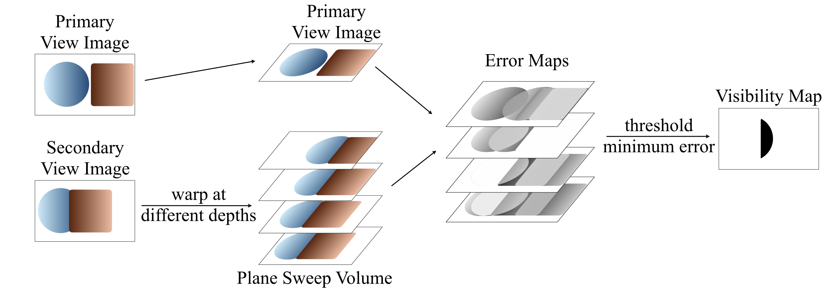
Figure 2. A toy example to illustrate the computation of visibility prior. The scene contains a blue sphere and a brown box and the relative pose between the views is a translation in $\mathbf{x}$ direction. The secondary view image is warped to the primary view at different depth planes to create a PSV and compared with the primary view image to obtain error maps. We observe that the brown square and the blue circle are matched better in the second and third planes respectively leading to lower error (denoted as white) in the respective error maps. The minimum error across all the planes is thresholded to obtain the visibility prior map corresponding to the primary view image. The right portion of the sphere which is occluded in the secondary view image is denoted in black in the visibility map.

3. NeRF Preliminaries

We first provide a brief introduction to NeRF and define the notations for subsequent use. A neural radiance field is an implicit representation of a scene using two multi-layer perceptrons (MLP). Given a set of images of a scene with corresponding camera poses, a pixel $\mathbf{q}$ is selected at random, and a ray $\mathbf{r}$ is passed from the camera center $\mathbf{o}$ through $\mathbf{q}$. Let $\mathbf{p}_{1},\mathbf{p}_{2},\ldots,\mathbf{p}_{N}$ be $N$ randomly sampled 3D points along $\mathbf{r}$. If $\mathbf{d}$ is the direction vector of $\mathbf{r}$ and $z_{i}$ is the depth of a 3D point $\mathbf{p}_{i}$, $i\in\{1,2,\ldots,N\}$, then $\mathbf{p}_{i}=\mathbf{o}+z_{i}\mathbf{d}$. An MLP $\mathcal{F}_{1}$ is trained to predict the volume density $\sigma_{i}$ at $\mathbf{p}_{i}$ as

(1) $$\sigma_{i},\mathbf{h}_{i} =\mathcal{F}_{1}(\mathbf{p}_{i}),$$

where $\mathbf{h}_{i}$ is a latent representation. A second MLP $\mathcal{F}_{2}$ then predicts the color using $\mathbf{h}_{i}$ and the viewing direction $\mathbf{v}=\mathbf{d}/\|\mathbf{d}\|$ as

(2) $$\mathbf{c}_{i} =\mathcal{F}_{2}(\mathbf{h}_{i},\mathbf{v}).$$

Let the distance between two consecutive samples $\mathbf{p}_{i}$ and $\mathbf{p}_{i+1}$ be $\delta_{i}=z_{i+1}-z_{i}$. The visibility or transmittance of $\mathbf{p}_{i}$ is then given by

(3) $$T_{i} =\exp\left(-\sum_{j=1}^{i-1}\delta_{j}\sigma_{j}\right).$$

The weight or contribution of $\mathbf{p}_{i}$ in rendering the color $\hat{\mathbf{c}}$ of pixel $\mathbf{q}$ is computed as

(4) $$w_{i}=T_{i}\left(1-\exp(-\delta_{i}\sigma_{i})\right)$$

to obtain

(5) $$\mathbf{\hat{c}} =\sum_{i=1}^{N}w_{i}\mathbf{c}_{i}.$$

The MLPs are trained using mean squared error loss with the true color $\mathbf{c}$ of $\mathbf{q}$ as

(6) $$\mathcal{L}_{mse}=\|\mathbf{c}-\mathbf{\hat{c}}\|^{2}.$$

Table 1. Quantitative results on RealEstate-10K dataset.

	learned	2 views			3 views			4 views
Model	prior	LPIPS ↓	SSIM ↑	PSNR ↑	LPIPS ↓	SSIM ↑	PSNR ↑	LPIPS ↓	SSIM ↑	PSNR ↑
InfoNeRF		0.6796	0.4653	12.30	0.6979	0.4024	11.15	0.6745	0.4298	11.52
DietNeRF	✓	0.5730	0.6131	15.90	0.5365	0.6190	16.60	0.5337	0.6282	16.89
RegNeRF		0.5307	0.5709	16.14	0.4675	0.6096	17.38	0.4831	0.6068	17.46
DS-NeRF		0.4273	0.7223	21.40	0.3930	0.7554	23.73	0.3961	0.7575	24.24
DDP-NeRF	✓	0.2527	0.7890	21.44	0.2240	0.8223	23.10	0.2190	0.8270	24.17
ViP-NeRF		0.1704	0.8087	24.48	0.1441	0.8505	27.21	0.1386	0.8588	28.13

Table 2. Quantitative results on NeRF-LLFF dataset.

	learned	2 views			3 views			4 views
Model	prior	LPIPS ↓	SSIM ↑	PSNR ↑	LPIPS ↓	SSIM ↑	PSNR ↑	LPIPS ↓	SSIM ↑	PSNR ↑
InfoNeRF		0.7561	0.2095	9.23	0.7679	0.1859	8.52	0.7701	0.2188	9.25
DietNeRF	✓	0.7265	0.3209	11.89	0.7254	0.3297	11.77	0.7396	0.3404	11.84
RegNeRF		0.4402	0.4872	16.90	0.3800	0.5600	18.62	0.3446	0.6056	19.83
DS-NeRF		0.4548	0.5068	17.06	0.4077	0.5686	19.02	0.3825	0.6016	20.11
DDP-NeRF	✓	0.4223	0.5377	17.21	0.4178	0.5610	17.90	0.3821	0.5999	19.19
ViP-NeRF		0.4017	0.5222	16.76	0.3750	0.5837	18.92	0.3593	0.6085	19.57

4. Method

We illustrate the outline of our model in Fig. 1. The core idea of our work is that when only a few multiview images are available for NeRF training, the visibility of a pixel in different views can be more reliably densely estimated as compared to its absolute depth. In this regard, we introduce visibility regularization to train the NeRF with sparse input views in Sec. 4.1. To impose the visibility regularization, we obtain a binary visibility prior map for every pair of input training images, which we explain in Sec. 4.2. Finally, to reduce the training time, we design a method to efficiently predict the visibility of a given pixel in different views in Sec. 4.3. Sec. 4.4 summarizes the various loss functions used in training our model.

4.1. Visibility Regularization

Recall from Sec. 3 that NeRF trains MLPs by picking a random pixel $\mathbf{q}$ and predicting the color of $\mathbf{q}$ using the MLPs and volume rendering. Without loss of generality, we refer to the view corresponding to the ray $\mathbf{r}$ passing through $\mathbf{q}$ as the primary view and choose any other view as a secondary view. NeRF then samples $N$ candidate 3D points, $\mathbf{p}_{1},\mathbf{p}_{2},\ldots,\mathbf{p}_{N}$, along $\mathbf{r}$. Let $T^{\prime}_{i}$ be the visibility of $\mathbf{p}_{i}$ from the secondary view, computed similar to Eq. 3. We define the visibility of pixel $\mathbf{q}$ in the secondary view, $t^{\prime}(\mathbf{q})$, as the weighted visibilities of all the candidate 3D points $\mathbf{p}_{i}$ analogous to Eq. 5 as

(7) $$t^{\prime}(\mathbf{q})=\sum_{i=1}^{N}w_{i}T^{\prime}_{i}\quad\in[0,1],$$

where $w_{i}$ are obtained through Eq. 4. We omit the dependence of $w_{i}$ and $T^{\prime}_{i}$ on $\mathbf{q}$ in the above equation for ease of reading. We obtain a prior $\tau^{\prime}(\mathbf{q})\in\{0,1\}$ on the visibility $t^{\prime}(\mathbf{q})$ as described in Sec. 4.2. We constrain the visibility $t^{\prime}(\mathbf{q})$ to match the prior $\tau^{\prime}(\mathbf{q})$. However, we find that the prior may be unreliable at pixels where $\tau^{\prime}=0$, as we describe in Sec. 4.2. Hence, we do not impose any visibility loss on such pixels and formulate our visibility prior loss as

(8) $$\mathcal{L}_{vip}(\mathbf{q})=\max(\tau^{\prime}(\mathbf{q})-t^{\prime}(\mathbf{q}),0).$$

Note that our loss function constrains the NeRF across pairs of views, unlike previous works which regularize (Roessle et al., 2022; Niemeyer et al., 2022) in a given view alone. We believe that this leads to a better regularization for synthesizing novel views.

4.2. Visibility Prior

Given primary and secondary views, our goal is to estimate whether every pixel in the primary view is also visible in the secondary view through a binary visibility prior $\tau^{\prime}(\mathbf{q})$. We employ plane sweep volumes to compute the visibility prior. We illustrate the computation of the visibility prior with a toy example in Fig. 2. Here, we warp the image in the secondary view to the primary view using the camera parameters at different depths varying between the near depth $z_{\min}$ and far depth $z_{\max}$. We sample $D$ depths uniformly in inverse depth similar to StereoMag (Zhou et al., 2018). The set of warped images is referred to as plane sweep volume (PSV) (Huang et al., 2018).

Let $I^{(1)}$ be the image in the primary view and $I_{k}^{(2)}$ be the set of $D$ warped images, where $k\in\{0,1,\ldots,D-1\}$ denotes the plane index. We then compute the error map $E_{k}$ of the warped secondary image with the primary image at each plane $k$ of the PSV as

(9) $$E_{k}=\|I^{(1)}-I_{k}^{(2)}\|_{1},$$

where the norm is computed across the color channels. We determine the visibility prior $\tau^{\prime}$ for pixel $\mathbf{q}$ by thresholding the minimum error across all the planes as

$$e(\mathbf{q}) =\min_{k}E_{k}(\mathbf{q}),$$

(10) $$\tau^{\prime}(\mathbf{q}) =\mathbbm{1}_{\{\exp{(-e(\mathbf{q})/\gamma)}>0.5\}},$$

where $\gamma$ is a hyper-parameter.

Intuitively, for a given pixel $\mathbf{q}$, a lower error in any of the planes indicates the presence of a matching pixel in the secondary view, i.e. $\mathbf{q}$ is visible in the secondary view. Note that this holds true when the intensity of pixels does not change significantly across views, which is typical for most of the objects in real-world scenes (Li et al., 2021). Consequently, the absence of a matching point across all the planes may indicate that $\mathbf{q}$ is not visible in the secondary view or $\mathbf{q}$ belongs to a highly specular object whose color varies significantly across different viewpoints. Thus, our prior is used to regularize the NeRF only in the first case above i.e. the pixels for which we find a match. Following the above procedure, we obtain the visibility prior for every pair of images obtained from the training set, by treating either image in the pair as the primary or the secondary view.

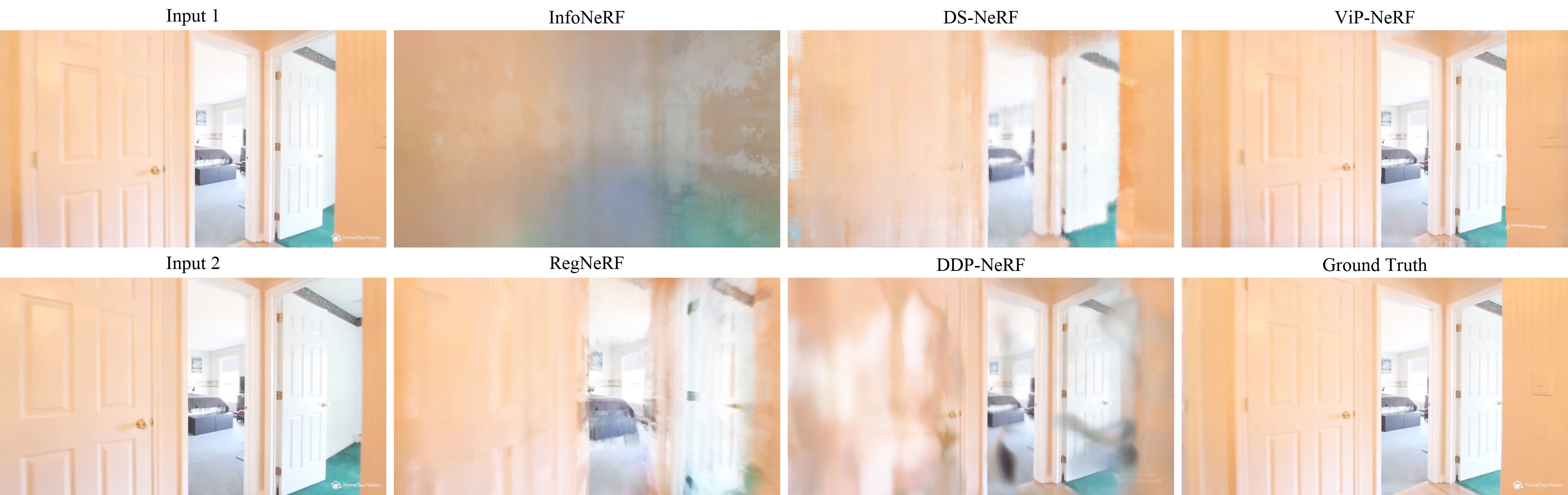
Figure 3. Qualitative examples on RealEstate-10K dataset with two input views. We observe that the predictions of ViP-NeRF are close to the ground truth, while those of other models suffer from various distortions. In particular, DDP-NeRF blurs regions of the frame near the left door and contains black floater artifacts.

4.3. Efficient Prediction of Visibility

Recall that imposing $\mathcal{L}_{vip}$ in Eq. 8 requires computing visibility $T^{\prime}_{i}$ in the secondary view for every $\mathbf{p}_{i}$. A naive approach to compute $T^{\prime}_{i}$ involves sampling up to $N$ points along a secondary ray from the secondary view camera origin to $\mathbf{p}_{i}$ and querying the NeRF MLP $\mathcal{F}_{1}$ for each of these points. Thus, obtaining $t^{\prime}(\mathbf{q})$ in Eq. 7 requires upto $N^{2}$ MLP queries, which increases the training time making it computationally prohibitive. We overcome this limitation by reformulating the NeRF MLP $\mathcal{F}_{2}$ to also output a view-dependent visibility of a given 3D point as,

(11) $$\mathbf{c}_{i},\hat{T}_{i}=\mathcal{F}_{2}(\mathbf{h}_{i},\mathbf{v});\quad\mathbf{c}^{\prime}_{i},\hat{T}^{\prime}_{i}=\mathcal{F}_{2}(\mathbf{h}_{i},\mathbf{v}^{\prime}_{i}),$$

where $\mathbf{v}^{\prime}_{i}$ is the viewing direction of the secondary ray. We use the MLP output $\hat{T}^{\prime}_{i}$ instead of $T^{\prime}_{i}$ in Eq. 7.

Note that to output $\hat{T}^{\prime}_{i}$, we need not query $\mathcal{F}_{1}$ again and can reuse $\mathbf{h}_{i}$ obtained from Eq. 1. We only need to query $\mathcal{F}_{2}$ additionally and since $\mathcal{F}_{2}$ is a single layer MLP and significantly smaller than $\mathcal{F}_{1}$, the additional computational burden is negligible. Thus, directly obtaining the secondary visibility $\hat{T}^{\prime}_{i}$ of $\mathbf{p}_{i}$ through Eq. 11 allows us to compute $t^{\prime}(\mathbf{q})$ in Eq. 7 using only $N$ queries of the MLP $\mathcal{F}_{1}$, as opposed to $N^{2}$ queries in the naive approach.

However, the use of $\hat{T}^{\prime}_{i}$ in place of $T^{\prime}_{i}$ regularizes the NeRF training only if the two quantities are close to each other. Thus, we introduce an additional loss to constrain the visibility $\hat{T}_{i}$ output by $\mathcal{F}_{2}$ to be consistent with the visibility $T_{i}$ computed using Eq. 3 as

(12) $$\mathcal{L}_{v}=\sum_{i=1}^{N}\left(\left(\text{SG}(T_{i})-\hat{T}_{i}\right)^{2}+\left(T_{i}-\text{SG}(\hat{T}_{i})\right)^{2}\right),$$

where $\text{SG}(\cdot)$ denotes the stop-gradient operation. The first term in the above loss function uses $T_{i}$ as a target and brings $\hat{T}_{i}$ closer to it. On the other hand, since $\hat{T}_{i}$ gets additionally updated directly based on the visibility prior, the second term helps transfer such updates to $\mathcal{F}_{1}$ more efficiently than backpropagation through $\mathcal{F}_{2}$.

4.4. Overall Loss

Similar to DS-NeRF (Deng et al., 2022), we also use the sparse depth given by an SfM model to supervise the NeRF as

(13) $$\mathcal{L}_{sd}=\|z-\hat{z}\|^{2},$$

where $z$ is the depth provided by the SfM model, $\hat{z}=\sum_{i}w_{i}z_{i}$ is the depth estimated by NeRF and $w_{i}$ are obtained in Eq. 4. Our overall loss for ViP-NeRF is a linear combination of the losses obtained in Eq. 6, Eq. 8, Eq. 12 and Eq. 13 as

(14) $$\mathcal{L}=\lambda_{1}\mathcal{L}_{mse}+\lambda_{2}\mathcal{L}_{sd}+\lambda_{3}\mathcal{L}_{vip}+\lambda_{4}\mathcal{L}_{v},$$

where $\lambda_{1},\lambda_{2},\lambda_{3}\text{ and }\lambda_{4}$ are hyper-parameters. We note that $\mathcal{L}_{vip}$ is always employed in conjunction with $\mathcal{L}_{v}$ to make the learning computationally tractable.

5. Experiments

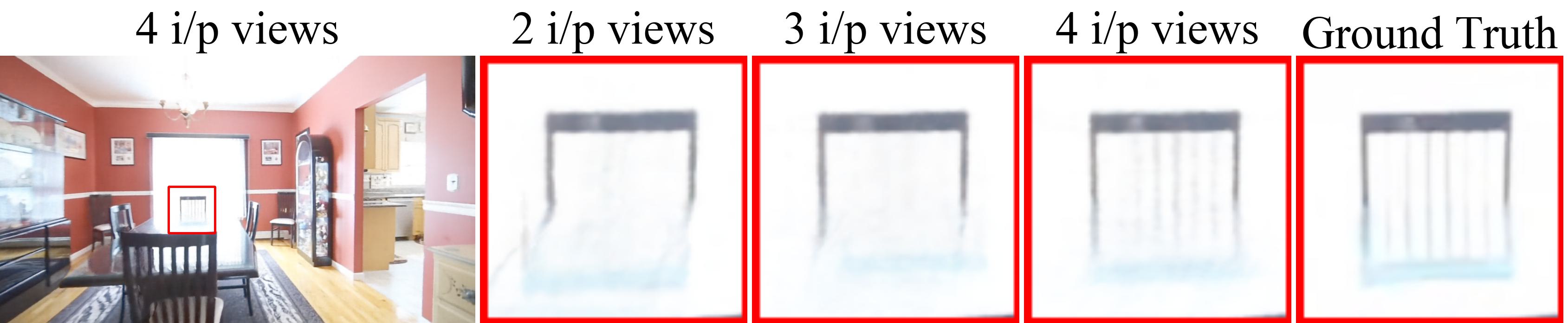
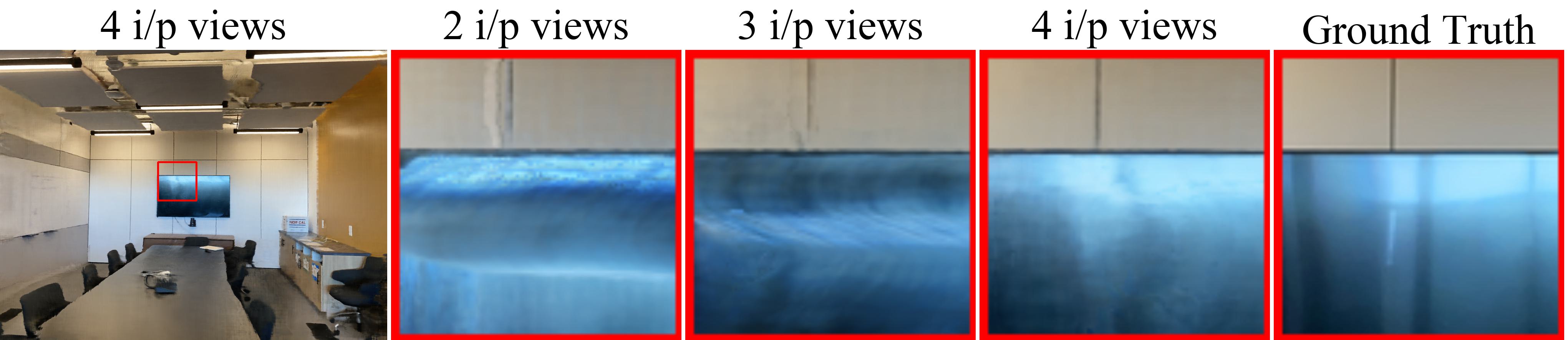
Figure 4. Qualitative examples on RealEstate-10K and NeRF-LLFF dataset with two, three, and four input views. We observe that ViP-NeRF models specular regions better as the number of input views increases. For example, in the first row, the reflection of the chair is better reconstructed as the number of views increases.

5.1. Evaluation Setup

We conduct experiments on two different datasets, namely RealEstate-10K and NeRF-LLFF. We evaluate all the models in the more challenging setup of 2, 3, or 4 input views, unlike prior work which use 9–18 input views (Jain et al., 2021; Roessle et al., 2022). The test set is retained to be the same across all different settings for both datasets.

RealEstate-10K (Zhou et al., 2018) dataset is commonly used to evaluate view synthesis models (Tucker and Snavely, 2020; Han et al., 2022) and contains videos of camera motion, both indoor and outdoor. The dataset also provides the camera intrinsics and extrinsics for all the frames. For our experiments, we choose 5 scenes from the test set, each containing 50 frames with a spatial resolution of $1024\times 576$. In each scene, we reserve every $10^{\text{th}}$ frame for training and use the remaining 45 frames for testing. Please refer to the supplementary for more details on the choice of scenes.

NeRF-LLFF (Mildenhall et al., 2019) dataset is used to evaluate the performance of various NeRF Models including sparse input NeRF models. It consists of 8 forward-facing scenes with a variable number of frames per scene at a spatial resolution of $1008\times 756$. Following RegNeRF (Niemeyer et al., 2022), we use every $8^{\text{th}}$ frame for testing. For training, we pick 2, 3 or 4 frames uniformly among the remaining frames following RegNeRF (Niemeyer et al., 2022).

Evaluation measures: We quantitatively evaluate the methods using LPIPS (Zhang et al., 2018), structural similarity (SSIM) (Wang et al., 2004), and peak signal to noise ratio (PSNR) measures. For LPIPS, we use the v0.1 release with the AlexNet (Krizhevsky et al., 2012) backbone as suggested by the authors.

Table 3. Comparison of reliability of priors used in different models. The reference visibility is obtained using NeRF trained with dense input views.

	RealEstate-10K			NeRF-LLFF
model	Prec. ↑	Rec. ↑	F1 ↑	Prec. ↑	Rec. ↑	F1 ↑
ViP-NeRF	0.97	0.83	0.89	0.82	0.85	0.83
DDP-NeRF	0.98	0.53	0.66	0.86	0.33	0.47

Table 4. Evaluation of depth estimated by different models with two input views. The reference depth is obtained using NeRF trained with dense input views. The depth RMSE on the two datasets are of different orders on account of different depth ranges.

	RealEstate-10K		NeRF-LLFF
model	RMSE ↓	SROCC ↑	RMSE ↓	SROCC ↑
ViP-NeRF	1.6411	0.7702	45.6314	0.6184
DDP-NeRF	1.7211	0.7544	46.6268	0.6136

5.2. Comparisons and Implementation Details

We compare the performance of our model with other sparse input NeRF models such as DDP-NeRF (Roessle et al., 2022) and DietNeRF (Jain et al., 2021) which use learned priors to constrain the NeRF training. We also compare with DS-NeRF (Deng et al., 2022), InfoNeRF (Kim et al., 2022), and RegNeRF (Niemeyer et al., 2022) that do not use learned priors. We train the models for 50k iterations on both datasets using the code provided by the respective authors.

For ViP-NeRF, we use Adam optimizer with a learning rate of 5e-4 that exponentially decays to 5e-6 following NeRF (Mildenhall et al., 2020). We set the loss weights such that the magnitudes of all the losses are of similar order after scaling. Specifically, we set $\lambda_{1}=1,\lambda_{2}=0.1,\lambda_{3}=0.001\text{ and }\lambda_{4}=0.1$. For visibility prior estimation, we set $D=64$ and $\gamma=10$. Since we require $\hat{T}^{\prime}_{i}$ to be close to $T^{\prime}_{i}$ while using $\hat{T}^{\prime}_{i}$ to compute $\mathcal{L}_{vip}$, we impose $\mathcal{L}_{vip}$ after 20k iterations. We train our models on a single NVIDIA RTX A4000 16GB GPU.

5.3. Results

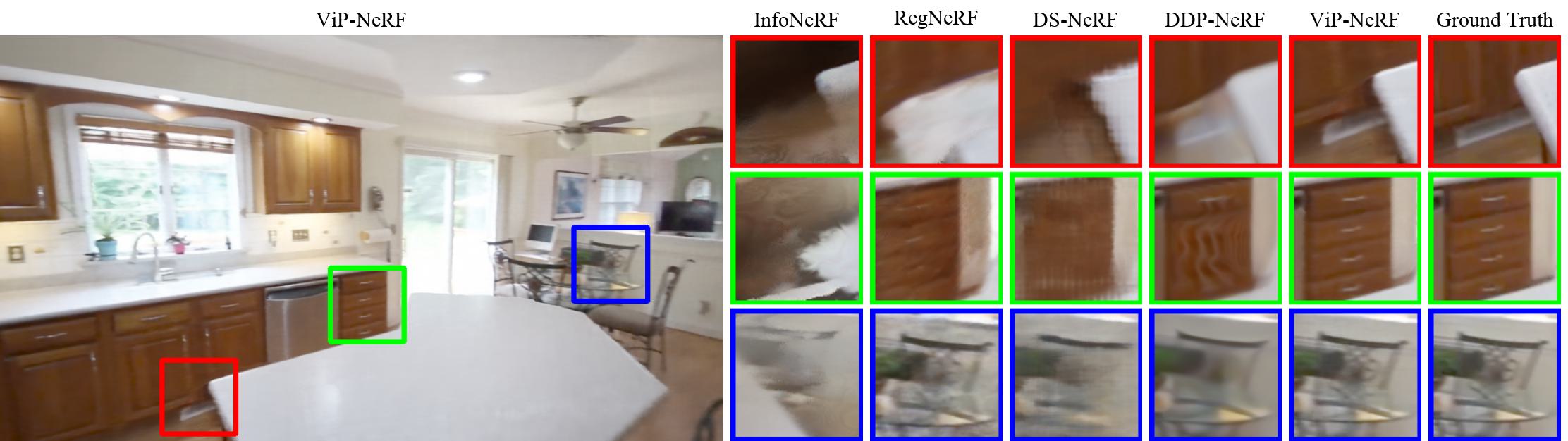
Figure 8. Qualitative examples on RealEstate-10K dataset with three input views. We find that ViP-NeRF is able to reconstruct novel views significantly better than the competing models. DDP-NeRF extends parts of the white table and fails to reconstruct the drawer handles accurately in the first and second examples. In the third example, DDP-NeRF fails to reconstruct thin objects in the chair.

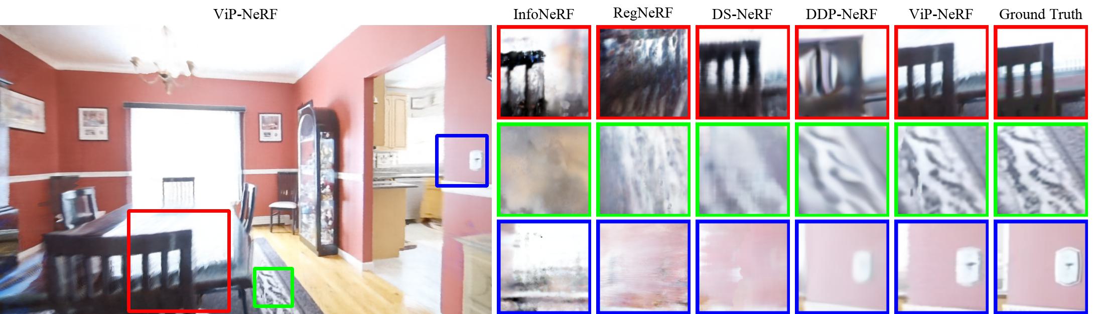
Figure 9. Qualitative examples on RealEstate-10K dataset with four input views. In the first example, DDP-NeRF fails to retain the structure of the chair while it blurs the texture of the carpet in the second example. We observe even more severe distortions among the predictions of other models.

We show the quantitative performance of ViP-NeRF and other competing models on RealEstate-10K and NeRF-LLFF datasets in Tabs. 1 and 2. Our model outperforms all the competing models, particularly in terms of the perceptual metric, LPIPS. ViP-NeRF even outperforms models such as DDP-NeRF and DietNeRF which involve pre-training on a large dataset. Fig. 3 shows qualitative comparisons on a scene from the RealEstate-10K dataset, where we observe significantly better synthesis by our model as compared to the competing models. We show more qualitative comparisons in Figs. 7, 8, 9 and 10 in the figure only pages at the end of this manuscript. In these samples, we find that ViP-NeRF removes most of the floater artifacts and successfully retains the shapes of objects.

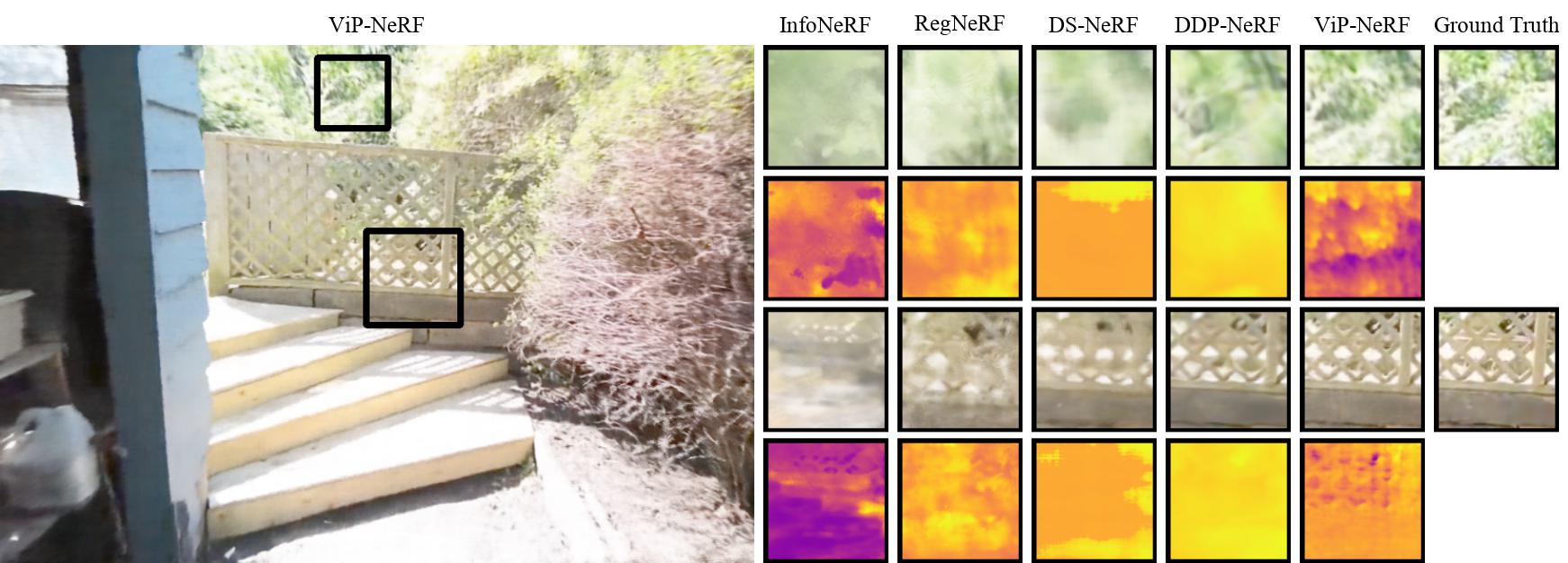
Figure 5. Estimated depth map on RealEstate-10K dataset with two input views. We find that ViP-NeRF is better in both frame synthesis and depth estimation compared to the competing models. For example, in the first row, the depth estimated by DDP-NeRF is smooth which may be leading to a loss of sharpness in synthesizing the shrubs. In contrast, ViP-NeRF predictions are sharper. For better visualization, we show inverse depth and normalize it to set the maximum value to unity.

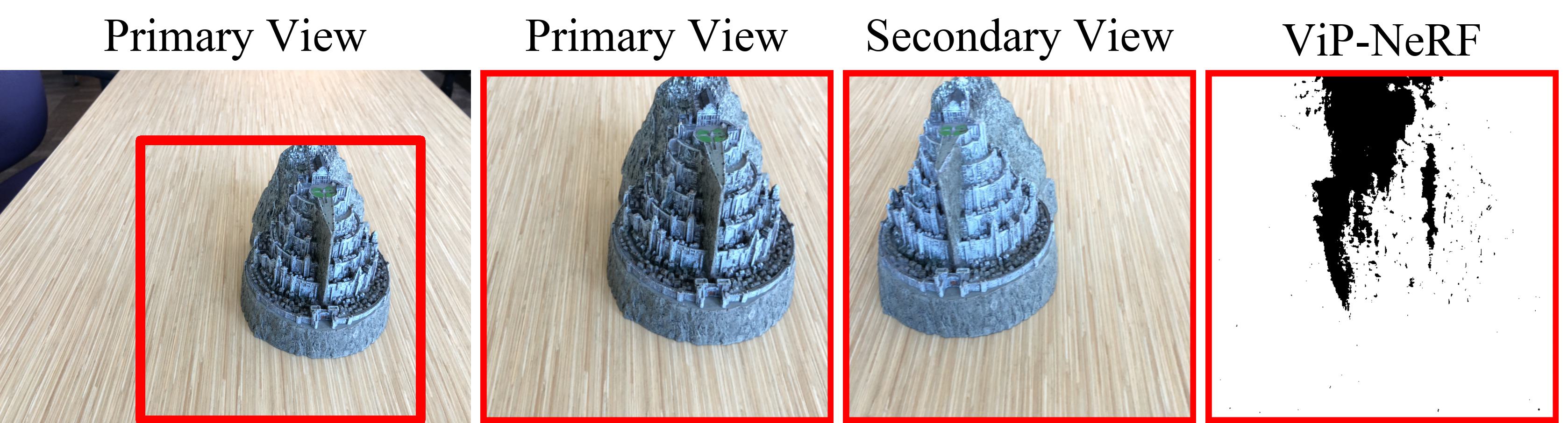
Figure 6. Visualization of the visibility map predicted by ViP-NeRF. White indicates the regions of the ‘Primary View’ which are visible in the ‘Secondary View’ and black indicates the occluded regions. From the primary and secondary views, we observe that the left part of the fortress and the neighboring portion of the wood are hidden in the secondary view. ViP-NeRF is able to reasonably determine the visible and occluded regions.

Table 5. Ablation experiments on both the datasets with two input views.

	RealEstate-10K		NeRF-LLFF
model	LPIPS ↓	SSIM ↑	LPIPS ↓	SSIM ↑
ViP-NeRF	0.1704	0.8087	0.4017	0.5222
w/o sparse depth	0.2754	0.7588	0.5056	0.4631
w/o dense visibility	0.4273	0.7223	0.4548	0.5068

In Fig. 4, we qualitatively compare the predictions of our model with different numbers of input views. We observe that ViP-NeRF estimates the geometry reasonably well with even two input views. However, with more input views, the performance of ViP-NeRF improves in reflective or specular regions. Fig. 6 visualizes the visibility map predicted by ViP-NeRF, where we observe that it is able to accurately predict the regions in the primary image which are visible and occluded in the secondary image.

Dense depth vs dense visibility: The key idea of our paper is that it may be possible to reliably estimate dense visibility than dense depth. From Tab. 1, we find that ViP-NeRF outperforms DDP-NeRF consistently, which indicates that the dense visibility prior we compute without any pre-training is superior to the learned dense depth prior used by DDP-NeRF. Further from Tab. 2, we observe that ViP-NeRF consistently improves over DS-NeRF in terms of LPIPS and SSIM, whereas DDP-NeRF does not. This may be due to the domain shift between the training dataset of DDP-NeRF and the LLFF dataset, resulting in no performance improvement over DS-NeRF. Thus, we conclude that augmenting sparse depth with dense visibility leads to better view synthesis performance than dense completion of the sparse depth. We further validate this conclusion by comparing the two priors in the following.

Validating priors: We compare the reliability of the dense visibility prior used in our model against the dense depth prior from DDP-NeRF. For this comparison, we convert the dense depth to visibility and compare it with the visibility prior of our approach. Specifically, we warp the image in the secondary view to the primary view using the dense depth prior and compute the visibility map similar to Eq. 10. We compare the visibility maps obtained using dense depth and our approach with the visibility map predicted by a NeRF model trained with dense input views. We evaluate the visibility maps in terms of precision, recall, and F1 score.

From Tab. 3, we observe that our approach significantly outperforms DDP-NeRF prior in terms of the recall and F1 score, while performing similarly in terms of precision. A high precision of our prior indicates that it makes very few mistakes when imposing $\mathcal{L}_{vip}$. On the other hand, a high recall shows that our prior is able to capture most of the visible regions where $\mathcal{L}_{vip}$ needs to be imposed. On the contrary, a low recall for the DDP-NeRF prior indicates that large regions that are actually visible in the secondary view are marked as occluded by the dense depth prior. Consequently, this indicates the presence of a large number of pixels with inaccurate depth in the prior of DDP-NeRF. Thus, we conclude that our visibility prior is more reliable than the dense depth prior from DDP-NeRF for training the NeRF.

As discussed in Sec. 1, visibility is related to relative depth, and thus a prior on visibility only constrains the relative depth ordering of the objects. On the other hand, the dense depth prior constrains the absolute depth, perhaps incorrectly. Thus the visibility prior provides more freedom to the NeRF in reconstructing the 3D geometry and is also more reliable compared to the depth prior. This may explain the superior performance of visibility regularization over dense depth regularization.

Evaluation of estimated depth: It is believed that better performance in synthesizing novel views is directly correlated with the accuracy of depth estimation (Deng et al., 2022). Thus, we compare our model with DDP-NeRF on their ability to estimate absolute depth correctly using root mean squared error (RMSE). We also evaluate the models on their ability to estimate the relative depth of the scene correctly using spearman rank-order correlation coefficient (SROCC) (Corder and Foreman, 2014), which computes the linear correlation between ranks of the estimated pixel depths with that of the ground truth depth. Due to the unavailability of ground truth depth on both the datasets, we train a NeRF model with dense input views and use its predicted depth as a pseudo ground truth. From Tab. 4, we observe that our model consistently outperforms DDP-NeRF both in terms of absolute and relative depth. Fig. 5 shows that the depth estimated by DDP-NeRF is smooth in textured regions, which may be leading to blur in the synthesized frame. In contrast, the dense visibility prior used in our model allows NeRF to predict sharp depth in such regions leading to sharper frame predictions.

Ablations: We analyze the contributions of dense visibility and sparse depth priors in ViP-NeRF, by disabling them one at a time. From Tab. 5 and Fig. 11(a), we find that removing either priors leads to a drop in performance on both the datasets. This suggests that the dense visibility prior may be providing information that is complementary to the sparse depth prior. For a more fine-grained analysis, we compare the LPIPS scores on individual scenes in Fig. 11(b). We observe that the addition of dense visibility prior over sparse depth prior leads to an improvement in the performance on all the scenes. Further, we find that our model with dense visibility prior alone is able to achieve impressive performance, especially on the RealEstate-10K dataset.

5.4. Limitations and Future Work

Our visibility prior constrains only the regions visible in at least two of the input views. As a result, we observe inaccurate depth estimation in the regions that are visible in only one of the input images. However, such regions account for a very small portion of the scene and reduce further with three or four input views. Further, ViP-NeRF may fail to synthesize disoccluded regions that can occur in sparse-input view synthesis, similar to RegNeRF. It would be interesting to explore the use of generative NeRF models such as pix2NeRF (Cai et al., 2022) to synthesize such disocclusions.

Our approach to estimating the visibility prior may not account for significant color changes that can occur when the scene contains highly specular surfaces. We do not impose any loss on such pixels. It would be interesting to analyze if pre-training a network on a large dataset to estimate visibility can provide more supervision in specular regions. Moreover, it would be interesting to see if pre-training a network to predict dense visibility generalizes better when compared to depth completion. Also, we observe in Tab. 2 that adding a new view leads to a significant improvement in performance as compared to adding new regularizations. Thus, one could explore hallucinating new views using generative models and use the hallucinated views for additional supervision.

6. Conclusion

We study the problem of training NeRFs in sparse input scenarios, where the NeRF tends to overfit the input views and learn incorrect geometry. We propose a prior on the visibility of pixels in other viewpoints to regularize the training and mitigate such errors. The visibility prior obtained using a plane sweep volume is more reliable as compared to the depth prior estimated using pre-trained networks. We reformulate the NeRF MLPs to additionally output visibility to compute the visibility prior loss in a time-efficient manner. ViP-NeRF achieves state-of-the-art performance on two commonly used datasets for novel view synthesis.

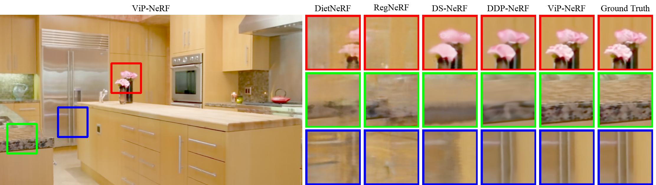
Figure 7. Qualitative examples on RealEstate-10K dataset with two input views. We observe sharp predictions by ViP-NeRF while predictions by other models suffer from blur and other artifacts. In particular, DDP-NeRF predictions contain blurred flowers (first row) and blurred tiles (second row).

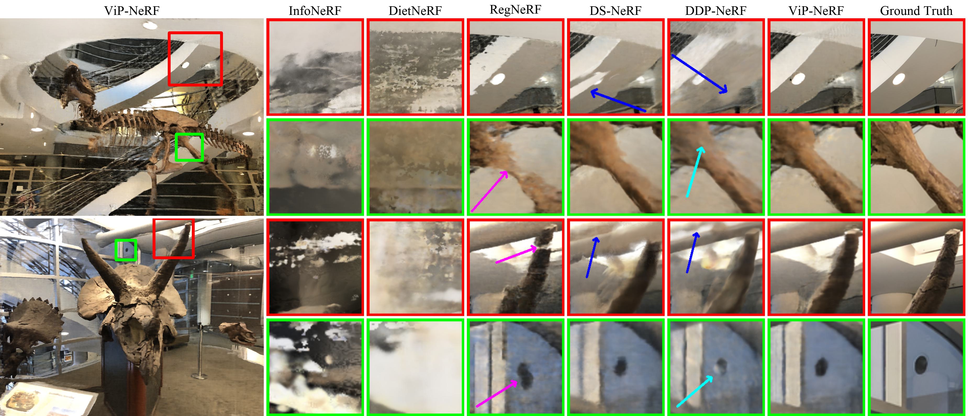
Figure 10. Qualitative examples on NeRF-LLFF dataset with two input views. In the first and third examples, we observe floater artifacts (blue arrows) in the predictions of DS-NeRF and DDP-NeRF, which are mitigated in the predictions of ViP-NeRF. We find that RegNeRF fails to capture thin t-rex bone in the second example and breaks the horn into two pieces in the third example (magenta arrows). Cyan arrows indicate color changes in the predictions of DDP-NeRF in the second and fourth examples. We note that predictions by our model do not suffer from the above described artifacts.

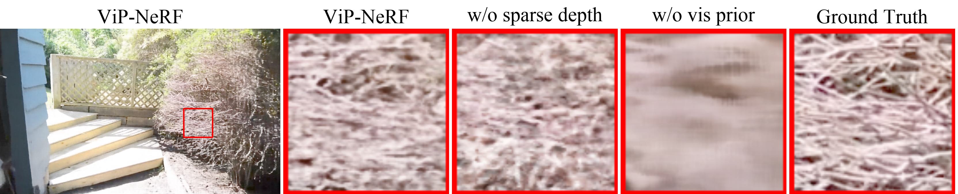
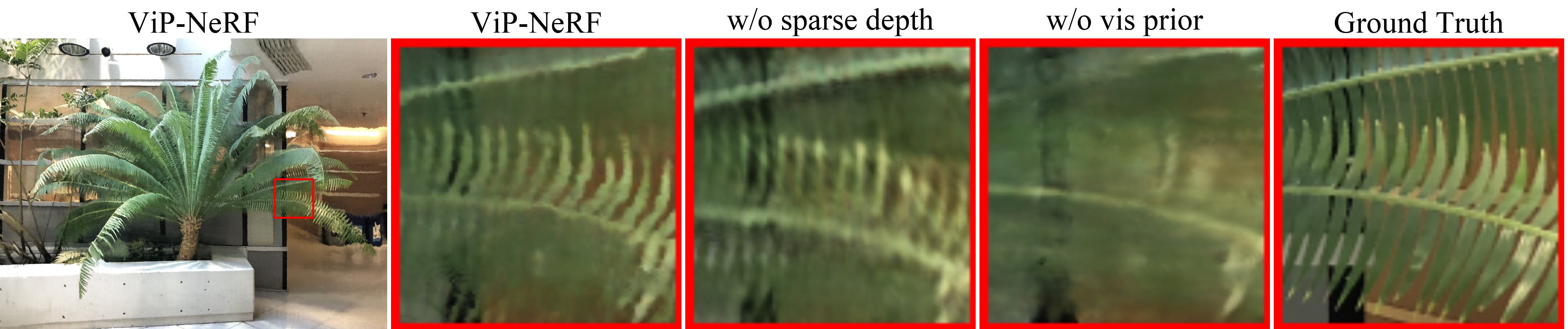
(a) Qualitative examples for ablations on RealEstate-10K and NeRF-LLFF dataset. We observe that the absence of dense visibility prior leads to significant blur in the predicted frames. While the reconstruction is reasonable without the sparse depth prior, we obtain the best reconstructions when using both the priors.

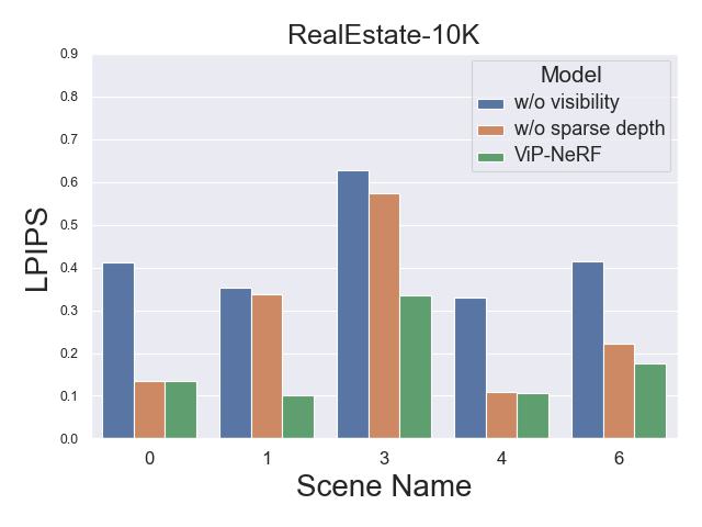
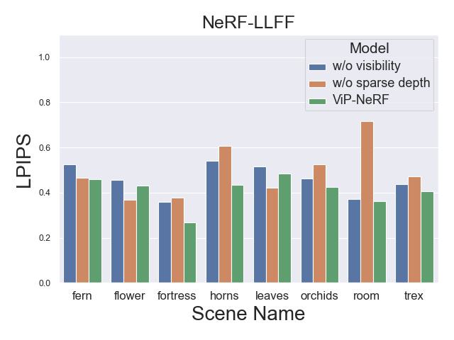
(b) Scene-wise LPIPS scores of ViP-NeRF and the ablated models. Note that lower LPIPS scores are better. ViP-NeRF performs better than both the ablated models in most cases leading to overall better performance.

Figure 11. Qualitative and quantitative comparisons of ablated models on both RealEstate-10K and NeRF-LLFF datasets.

Supplement

The contents of this supplement include

1. Details of RealEstate-10K dataset.

2. Implementation details of the competing sparse input NeRF models.

3. Comparisons on DTU dataset.

4. Video examples on RealEstate-10K and NeRF-LLFF datasets.

5. Additional comparisons between ViP-NeRF and DDP-NeRF.

6. Additional analysis.

Appendix A Dataset Details

RealEstate-10K (Zhou et al., 2018) is a large database consisting of about 80,000 video segments, each containing more than 30 frames. This dataset was proposed to train traditional deep learning models which require training on a large number of videos and hence the dataset is further divided into train and test splits. Since NeRF based models optimize the networks on individual scenes, we select five videos from the test set to evaluate the NeRF models. For easy reference, we rename the videos as scene numbers starting from zero. The dataset provides only links to the videos on YouTube and hence we discard the videos which are no longer available. Further, we also discard the videos which are less than 50 frames in length. We then select the first five videos and choose a random segment of 50 frames within the videos. In Tab. 6, we provide the mapping between the original name of the videos we selected and the updated names, along with the timestamp of the first frame in the video segment. Please refer to  Zhou et al. (2018) for more details on obtaining the data.

In each scene, we reserve 5 frames for training and use the remaining 45 frames for testing. Specifically, frames 10, 20, 30, 0 and 40 are reserved for training. For training with $n$ views, we choose the first $n$ frames from the above list.

Table 6. Original name of RealEstate-10K videos we selected for experiments and their updated names.

Original Name	Updated Name	Timestamp
000c3ab189999a83	0	53453400
000db54a47bd43fe	1	227894333
0017ce4c6a39d122	3	46012000
002ae53df0e0afe2	4	61144000
0043978734eec081	6	54387667

Appendix B Implementation Details

We use the official code releases by the respective authors and train the models on both RealEstate-10K and NeRF-LLFF datasets (Mildenhall et al., 2019). In the following, we provide details of any changes we make on top of the respective code releases.

InfoNeRF (Kim et al., 2022): The code release for InfoNeRF uses test viewpoints during training. For a fair comparison, we replace the test poses with poses interpolated from train poses.

RegNeRF (Niemeyer et al., 2022): We found an inconsistency between the description in the paper and the implementation (possibly a bug) in RegNeRF code, where they use only a single hallucinated view instead of multiple. We fix this and train the RegNeRF model.

Appendix C Comparisons on DTU Dataset

Table 7. Quantitative results on DTU dataset. RegNeRF+ uses test camera poses during training.

Model	learnt prior	LPIPS ↓	SSIM ↑	PSNR ↑
InfoNeRF		0.6649	0.2659	8.67
DietNeRF	✓	0.7686	0.2790	7.36
RegNeRF		0.7808	0.2327	7.25
RegNeRF+		0.4378	0.5310	12.73
DS-NeRF		0.5136	0.4841	11.99
DDP-NeRF	✓	0.5542	0.4544	11.40
ViP-NeRF		0.4876	0.5057	12.04

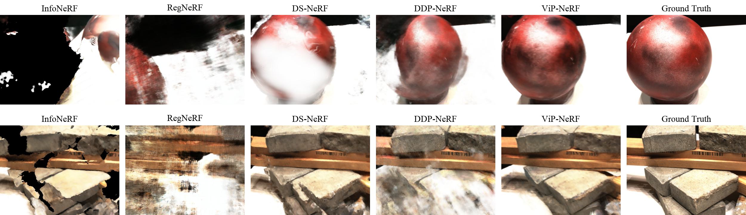
Figure 12. Qualitative examples on DTU dataset. We observe various distortions among the predictions by competing models. For example, in the second row, the DS-NeRF prediction has a ghosting artifact in one of the bricks. However, predictions by our model are significantly closer to the ground truth.

DTU (Aanæs et al., 2016) is a commonly used benchmark dataset for conditional NeRF models (Yu et al., 2021; Chen et al., 2021). Nonetheless, a few sparse input NeRF models benchmark on the DTU dataset as well. We use the train and test sets defined by pixelNeRF (Yu et al., 2021). Specifically, there are 15 scenes and around 49 frames per scene of which 40 frames are used for testing, and 9 frames are reserved for training.

We found that RegNeRF uses the test viewpoints as the hallucinated viewpoints for training on DTU scenes. However, this would be an unfair comparison since other models including ours do not use test camera poses during training. Hence we remove such viewpoints and train the RegNeRF model. Nonetheless, we report the performance of RegNeRF that uses test views during training as ‘RegNeRF+’ in Tab. 7.

We show quantitative comparisons between the competing models in Tab. 7 and qualitative comparisons in Fig. 12. ViP-NeRF outperforms all the competing models that do not use test camera poses during training, including DDP-NeRF and DietNeRF which employ pre-training. Even qualitatively, we find that the predictions of ViP-NeRF are closer to the ground truth without many artifacts seen in the predictions of the other models.

Appendix D Video Comparisons

Along with this supplementary, we attach a few videos to compare ViP-NeRF with the competing models such as DS-NeRF (Deng et al., 2022), DDP-NeRF (Roessle et al., 2022) and RegNeRF (Niemeyer et al., 2022). Kindly use the attached ‘VideoSamples.html’ file to view all the videos in a single browser window.

Appendix E Additional Comparisons

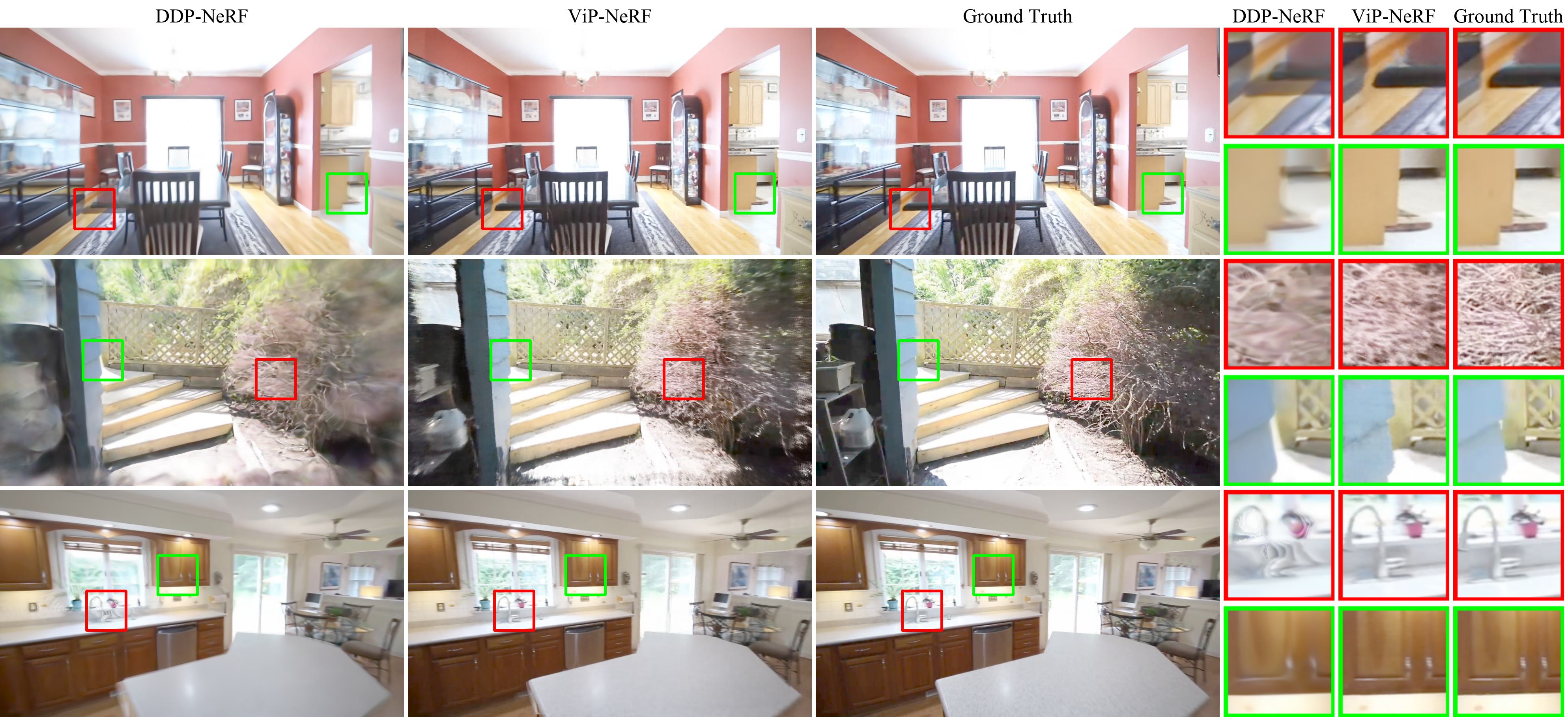
Figure 13. Qualitative examples on RealEstate-10K dataset with two input views. In the first example, we see artifacts such as ghosting and blur in the frame predicted by DDP-NeRF. In the second example, we observe that DDP-NeRF infers incorrect geometry due to which the objects are placed incorrectly in the synthesized view. However, the predictions by ViP-NeRF do not suffer from such artifacts and are significantly sharper.

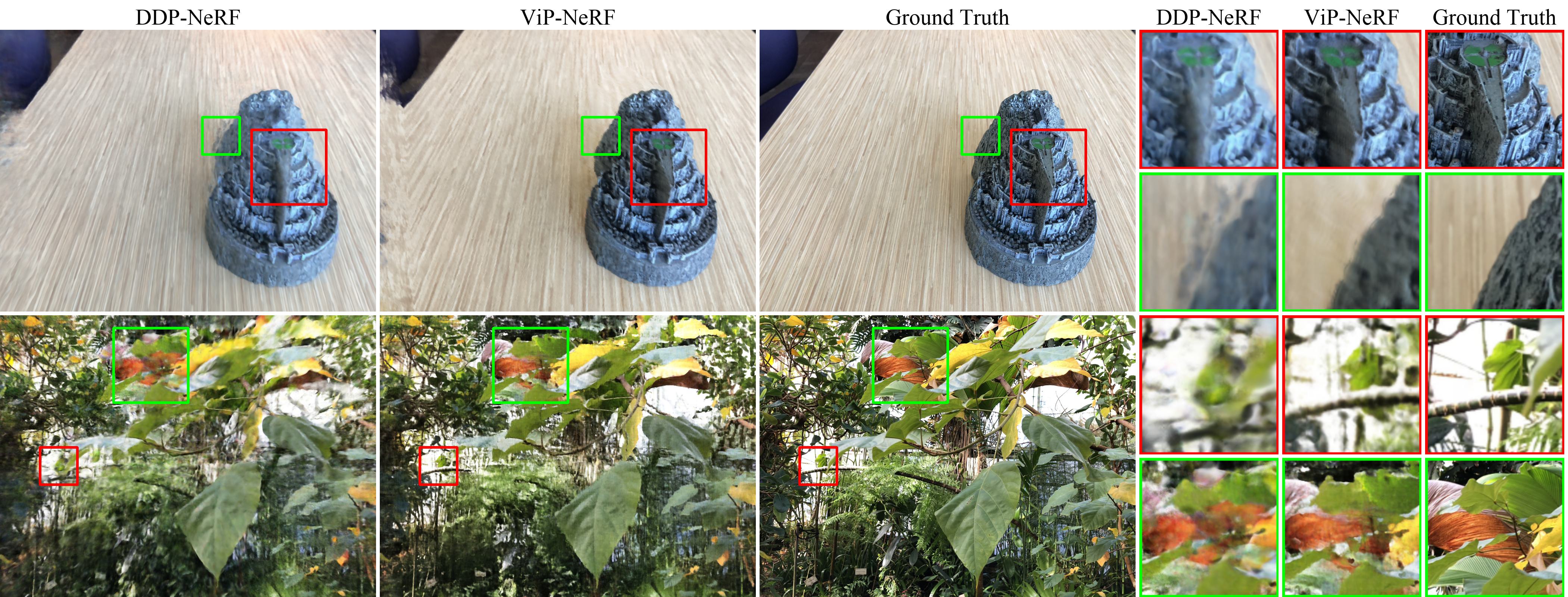
Figure 14. Qualitative examples on NeRF-LLFF dataset with three input views. In the first example, we find that DDP-NeRF prediction has a different global color than the ground truth. In addition, the angle of the sharp triangular object on the fortress is changed. We also observe floating blue clouds outside the fortress and blur in other regions. In the second example, we notice that DDP-NeRF is unable to infer the positions of the objects (horizontal stem and the orange leaf) correctly and instead places them at incorrect positions or breaks them into multiple parts. On the other hand, ViP-NeRF is able to synthesize the novel views reasonably well.

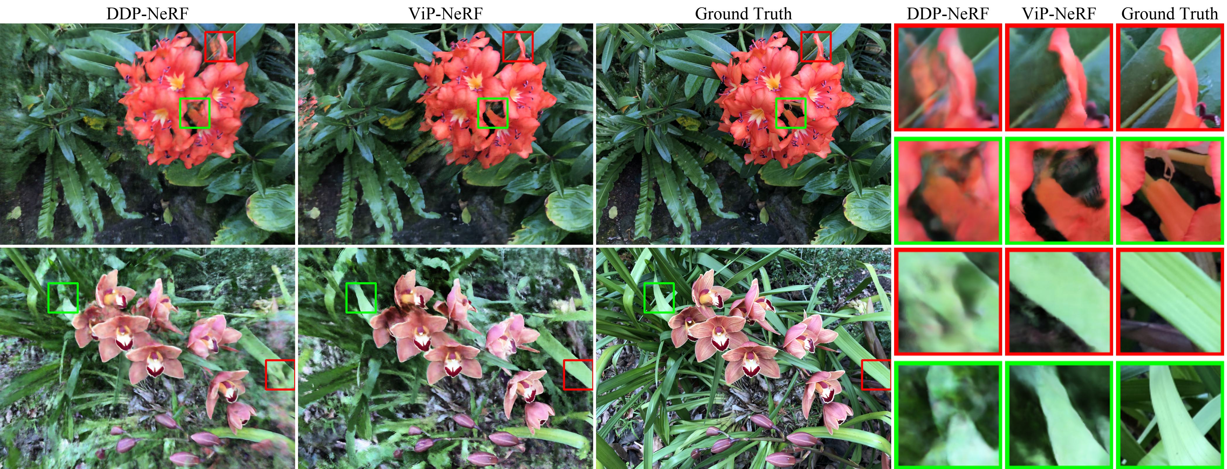
Figure 15. Qualitative examples on NeRF-LLFF dataset with four input views. We find that DDP-NeRF predictions contain floaters (orange in the first example and black in the second), whereas ViP-NeRF predictions are devoid of such artifacts. We also observe that ViP-NeRF finds difficulty in synthesizing disoccluded regions such as the flower stem in the first example. Nonetheless, ViP-NeRF predicts plausible solutions in such cases.

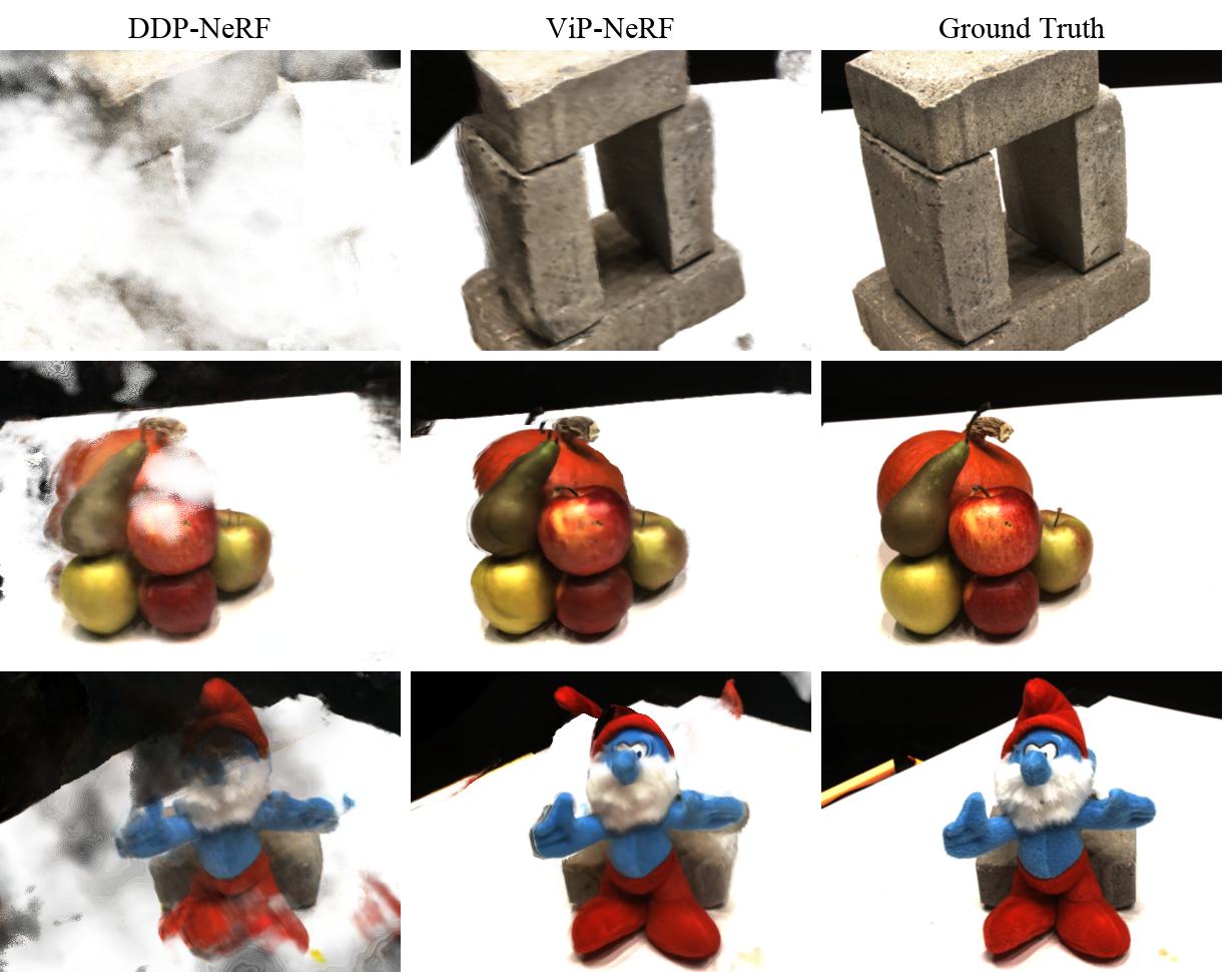
Figure 16. Qualitative examples on DTU dataset with two input views. DDP-NeRF predictions contain significant floating clouds in all three examples, whereas ViP-NeRF produces more realistic novel views.

Here, we show more comparisons with the second-best-performing model, DDP-NeRF, on both datasets. Specifically, out of 5 scenes from RealEstate-10K, Figs. 3 and 7 in the main paper show the comparisons on two of the scenes. Fig. 13 shows qualitative comparisons on the remaining three scenes. We observe that ViP-NeRF synthesizes superior quality frames compared to DDP-NeRF in all the scenes. On the NeRF-LLFF dataset, the figures in the main paper show ViP-NeRF predictions on 4 out of 8 scenes in the dataset. Figs. 14 and 15 shows ViP-NeRF predictions on the remaining four scenes in the NeRF-LLFF dataset.

Fig. 10 in the main paper shows qualitative comparisons with two input views on the NeRF-LLFF dataset. Figs. 14 and 15 show qualitative comparisons with three and four input views, respectively. From the figures, we observe that ViP-NeRF synthesizes sharper frames as compared to DDP-NeRF while maintaining better structures of the objects. Finally, Fig. 16 shows more comparisons with DDP-NeRF on the DTU dataset. We find that while ViP-NeRF synthesizes plausible frames, DDP-NeRF predictions suffer from floating white/black clouds that occlude the objects of interest.

In Tabs. 9, 10, 11, 12, 13 and 14, we provide scene-wise quantitative performance comparisons.

Appendix F Additional Analysis

F.1. PSV based Dense Depth Prior

Table 8. Comparison between NeRF models trained with visibility and depth priors obtained using plane sweep volume.

	RealEstate-10K		NeRF-LLFF
model	LPIPS ↓	SSIM ↑	LPIPS ↓	SSIM ↑
ViP-NeRF	0.1704	0.8087	0.4017	0.5222
DS-NeRF + PSV dense depth	0.7453	0.4247	0.6238	0.3878

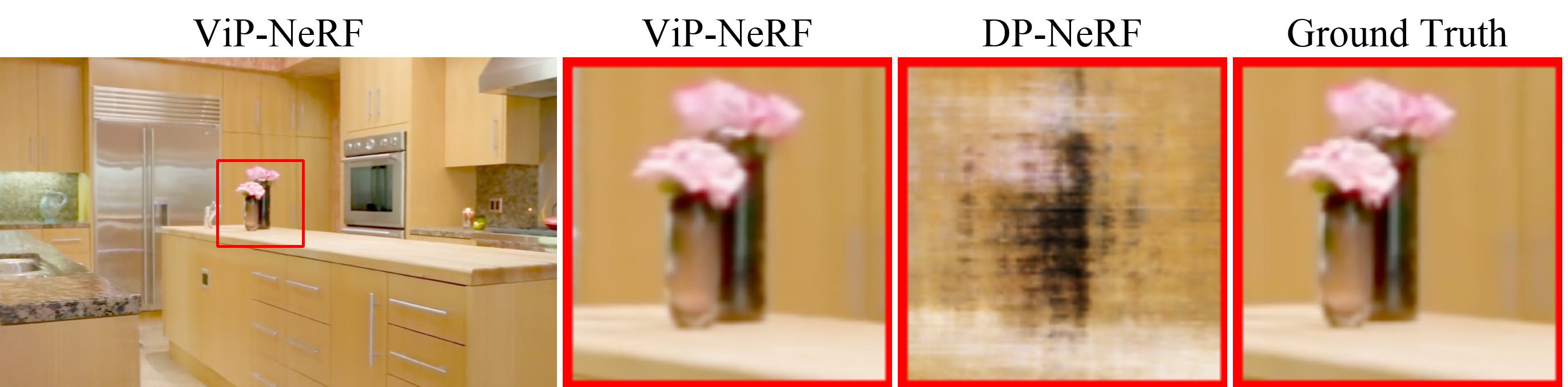
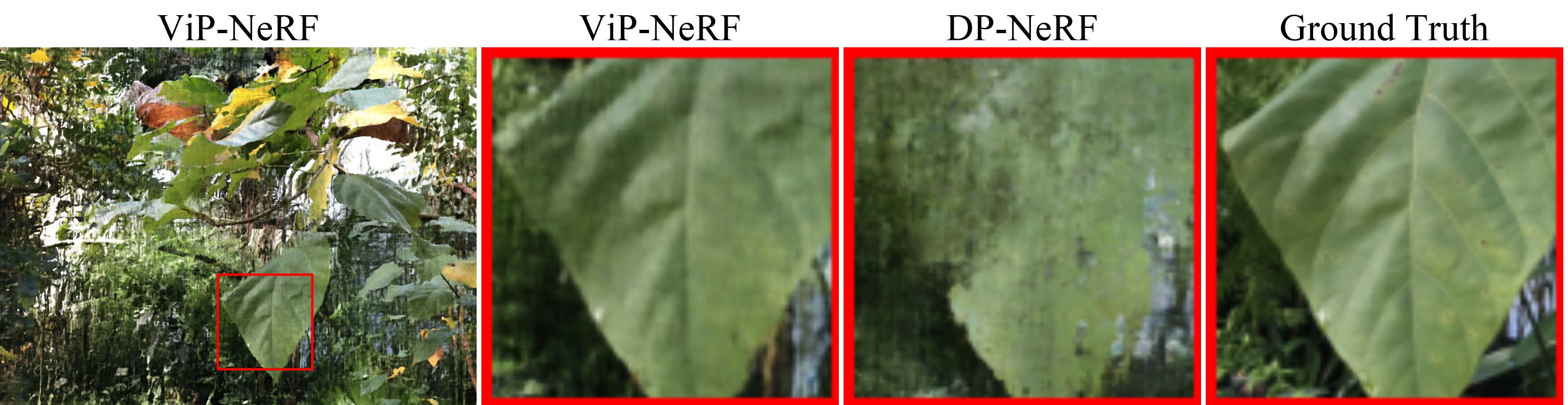
Figure 17. Qualitative examples on RealEstate-10K and NeRF-LLFF datasets with visibility and depth prior (DP-NeRF) obtained using our method. We observe significant distortions in the predictions of DP-NeRF due to unreliable depth prior.

Here, we ask whether the improvement in view synthesis performance is because the visibility prior can be reliably estimated or due to the use of plane sweep volumes. To answer this, we experiment with obtaining a dense depth prior using the plane sweep volume similar to our visibility map computation. Specifically, we estimate dense depth as $z_{p}(\mathbf{q})=\arg\min_{k}E_{k}(\mathbf{q})$ similar to Eq. 10 and use it to supervise NeRF similar to Eq. 13. We show the quantitative and qualitative performance of this model in Tab. 8 and Fig. 17, where we find that its performance significantly deteriorates. This supports our hypothesis that estimating depth accurately is a very hard problem that may require pre-training on a large dataset, but reliably estimating visibility appears to be relatively easier.

F.2. Distant Views

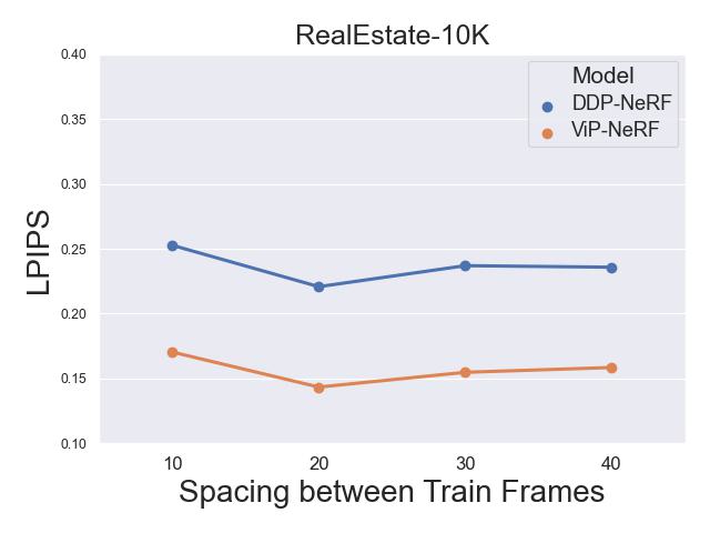
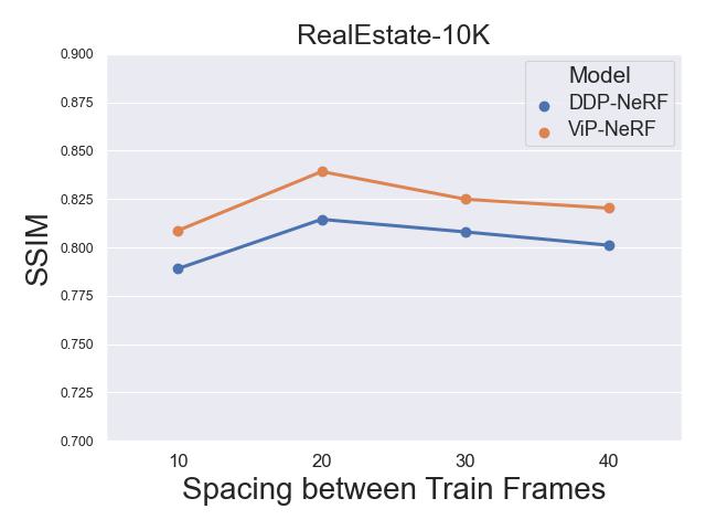
Figure 18. Quantitative comparison of the performance of DDP-NeRF and ViP-NeRF models with increasing distance between the training views. The x-axis denotes the frames skipped between the two training frames.

To understand how the performance of ViP-NeRF varies when the training images are farther apart with more occlusions, we train ViP-NeRF with 2 input views that are 10, 20, 30, and 40 frames apart on the RealEstate-10K dataset. We show the performance of ViP-NeRF in terms of LPIPS and SSIM in Fig. 18. For reference, we also conduct a similar experiment with DDP-NeRF and report its performance. We note that the performance of ViP-NeRF stays relatively stable across different settings. We observe a small improvement in performance initially, which may be due to the availability of new regions during training when the train views are spread more apart. However, the performance tends to drop in small amounts with a further increase in distance between the training views. Further, ViP-NeRF outperforms DDP-NeRF in all cases.

F.3. Accuracy of Predicted Visibility

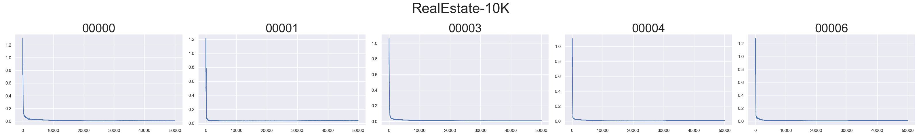
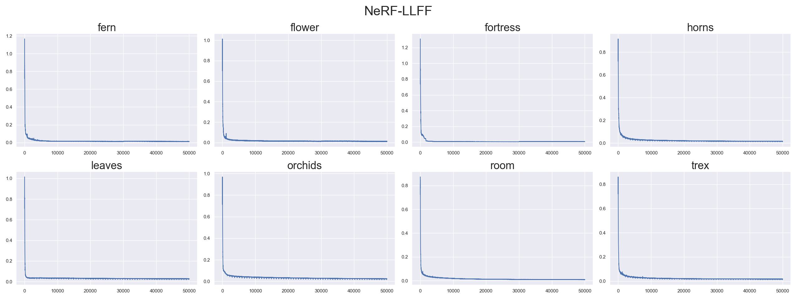
Figure 19. Loss curves of $\mathcal{L}_{v}$ during training on individual scenes of both RealEstate-10K and NeRF-LLFF datasets.

Recall that we use Eq. 12 during training to enforce the visibility $\hat{T}_{i}$ output by $\mathcal{F}_{2}$ to be consistent with the visibility $T_{i}$ computed by volume rendering. In Fig. 19, we plot $\mathcal{L}_{v}$ against the iteration number as the training progresses. We observe that the loss uniformly decreases to a very small value close to zero indicating that $\hat{T}_{i}$ and $T_{i}$ are indeed close to each other. This helps effective imposition of our visibility prior.

Appendix G Performance on Individual Scenes

In Tabs. 9, 10, 11, 12, 13 and 14, we report the performance of various models on individual scenes.

Table 9. Per-scene performance of various models with two input views on RealEstate-10K dataset. The three rows show LPIPS, SSIM, and PSNR scores, respectively.

model \ scene name	0	1	3	4	6	average
InfoNeRF	0.6545 0.4863 11.85	0.5037 0.7458 16.19	0.7386 0.3002 11.59	0.7982 0.3990 10.55	0.7033 0.3953 11.32	0.6796 0.4653 12.30
DietNeRF	0.6242 0.5743 13.16	0.4765 0.8298 18.13	0.7154 0.3065 12.11	0.5885 0.6632 16.86	0.4604 0.6919 19.22	0.5730 0.6131 15.90
RegNeRF	0.5212 0.5416 14.83	0.4305 0.8163 19.11	0.6050 0.2549 12.88	0.5427 0.6797 17.78	0.5542 0.5618 16.13	0.5307 0.5709 16.14
DS-NeRF	0.4128 0.7128 18.99	0.3535 0.8715 23.35	0.6269 0.4210 17.08	0.3298 0.8354 25.48	0.4133 0.7705 22.10	0.4273 0.7223 21.40
DDP-NeRF	0.2265 0.7985 20.79	0.2081 0.9222 22.16	0.4788 0.4663 16.89	0.1350 0.8964 24.43	0.2150 0.8615 22.91	0.2527 0.7890 21.44
ViP-NeRF w/o sparse depth	0.1358 0.8807 25.54	0.3363 0.8456 19.89	0.5723 0.3422 13.26	0.1100 0.9070 27.98	0.2225 0.8186 24.48	0.2754 0.7588 22.23
ViP-NeRF	0.1351 0.8802 25.03	0.1008 0.9425 26.81	0.3348 0.4567 17.05	0.1053 0.9085 27.91	0.1762 0.8558 25.60	0.1704 0.8087 24.48

Table 10. Per-scene performance of various models with three input views on RealEstate-10K dataset. The three rows show LPIPS, SSIM, and PSNR scores, respectively.

model \ scene name	0	1	3	4	6	average
InfoNeRF	0.7226 0.3806 10.07	0.6075 0.5669 13.06	0.6846 0.2155 10.09	0.7916 0.3991 10.82	0.6831 0.4496 11.70	0.6979 0.4024 11.15
DietNeRF	0.5565 0.5841 14.86	0.5400 0.7861 16.83	0.6475 0.3068 12.56	0.5258 0.7022 18.11	0.4126 0.7156 20.65	0.5365 0.6190 16.60
RegNeRF	0.4885 0.5625 15.16	0.3832 0.8200 20.11	0.5947 0.2852 13.41	0.5123 0.6851 18.57	0.3585 0.6951 19.67	0.4675 0.6096 17.38
DS-NeRF	0.3302 0.7772 22.09	0.3241 0.8902 26.61	0.5925 0.4540 18.30	0.3245 0.8460 26.94	0.3939 0.8096 24.70	0.3930 0.7554 23.73
DDP-NeRF	0.1868 0.8475 22.17	0.1644 0.9406 23.53	0.4665 0.5229 17.94	0.1067 0.9159 27.46	0.1955 0.8848 24.39	0.2240 0.8223 23.10
ViP-NeRF w/o sparse depth	0.1022 0.9046 27.64	0.3194 0.8284 21.04	0.3119 0.5611 18.77	0.0720 0.9277 31.61	0.1252 0.9157 29.39	0.1861 0.8275 25.69
ViP-NeRF	0.0977 0.9094 27.59	0.1302 0.9408 28.31	0.3083 0.5515 18.59	0.0682 0.9319 32.15	0.1163 0.9190 29.40	0.1441 0.8505 27.21

Table 11. Per-scene performance of various models with four input views on RealEstate-10K dataset. The three rows show LPIPS, SSIM, and PSNR scores, respectively.

model \ scene name	0	1	3	4	6	average
InfoNeRF	0.6386 0.5111 12.46	0.6315 0.4900 10.99	0.7153 0.2117 9.72	0.7993 0.3767 10.13	0.5879 0.5596 14.28	0.6745 0.4298 11.52
DietNeRF	0.5724 0.5974 14.45	0.4908 0.8224 18.75	0.6502 0.3031 12.89	0.5386 0.6964 17.85	0.4164 0.7219 20.50	0.5337 0.6282 16.89
RegNeRF	0.5054 0.5577 15.32	0.3902 0.8200 20.27	0.6256 0.2834 13.54	0.5229 0.6775 18.29	0.3711 0.6952 19.87	0.4831 0.6068 17.46
DS-NeRF	0.3657 0.7671 22.54	0.3161 0.8971 27.41	0.6193 0.4562 18.65	0.3039 0.8517 27.44	0.3755 0.8152 25.17	0.3961 0.7575 24.24
DDP-NeRF	0.1834 0.8479 22.26	0.1307 0.9490 26.08	0.4746 0.5394 18.65	0.1049 0.9161 28.81	0.2015 0.8828 25.04	0.2190 0.8270 24.17
ViP-NeRF w/o sparse depth	0.1022 0.9046 27.64	0.3194 0.8284 21.04	0.3119 0.5611 18.77	0.0720 0.9277 31.61	0.1252 0.9157 29.39	0.1861 0.8275 25.69
ViP-NeRF	0.0977 0.9094 27.59	0.1302 0.9408 28.31	0.3083 0.5515 18.59	0.0682 0.9319 32.15	0.1163 0.9190 29.40	0.1441 0.8505 27.21

Table 12. Per-scene performance of various models with two input views on NeRF-LLFF dataset. The three rows show LPIPS, SSIM, and PSNR scores, respectively.

model \ scene name	fern	flower	fortress	horns	leaves	orchids	room	trex	average
InfoNeRF	0.7805 0.2635 11.00	0.6880 0.1890 10.97	0.8156 0.1808 6.48	0.7649 0.2020 8.86	0.6422 0.0987 9.47	0.6908 0.1108 9.43	0.8044 0.3757 10.76	0.7941 0.2115 8.44	0.7561 0.2095 9.23
DietNeRF	0.7663 0.2883 12.30	0.6935 0.2590 12.18	0.6621 0.4424 14.22	0.7574 0.2819 10.71	0.6720 0.1196 10.58	0.7256 0.1470 10.57	0.7674 0.5153 13.09	0.7496 0.3674 11.30	0.7265 0.3209 11.89
RegNeRF	0.5067 0.4681 16.51	0.4408 0.5067 16.92	0.3838 0.4621 20.53	0.5301 0.4277 15.91	0.3590 0.3637 14.51	0.4595 0.3018 13.88	0.3955 0.7306 18.59	0.4308 0.5388 16.69	0.4402 0.4872 16.90
DS-NeRF	0.5249 0.4681 16.69	0.4578 0.4455 16.17	0.3591 0.6316 23.10	0.5395 0.4816 16.64	0.5174 0.2429 12.68	0.4614 0.3190 13.86	0.3727 0.7607 18.94	0.4386 0.5295 15.85	0.4548 0.5068 17.06
DDP-NeRF	0.4715 0.4940 17.35	0.4803 0.4535 16.18	0.1888 0.7600 22.77	0.4973 0.5167 17.10	0.5550 0.2282 12.65	0.4438 0.3682 15.12	0.3290 0.7572 18.68	0.4660 0.5358 15.76	0.4223 0.5377 17.21
ViP-NeRF w/o sparse depth	0.4665 0.4719 16.60	0.3673 0.5044 16.78	0.3779 0.5286 21.22	0.6068 0.4279 15.65	0.4210 0.3575 14.76	0.5252 0.2913 14.21	0.7174 0.5191 13.76	0.4706 0.5241 16.50	0.5056 0.4631 16.28
ViP-NeRF	0.4605 0.4586 16.45	0.4297 0.4355 14.65	0.2689 0.6869 22.36	0.4356 0.5353 17.25	0.4842 0.2172 11.90	0.4238 0.3592 14.21	0.3626 0.7371 18.11	0.4052 0.5383 16.13	0.4017 0.5222 16.76

Table 13. Per-scene performance of various models with three input views on NeRF-LLFF dataset. The three rows show LPIPS, SSIM, and PSNR scores, respectively.

model \ scene name	fern	flower	fortress	horns	leaves	orchids	room	trex	average
InfoNeRF	0.8583 0.2144 7.51	0.6949 0.2308 10.75	0.8272 0.1680 5.22	0.7555 0.1800 8.87	0.6518 0.1083 9.92	0.7121 0.0834 8.28	0.8312 0.2911 8.94	0.7885 0.1768 8.75	0.7679 0.1859 8.52
DietNeRF	0.7977 0.3207 12.01	0.6705 0.3052 13.08	0.6984 0.4098 12.37	0.7458 0.2946 11.10	0.6672 0.1266 10.57	0.7478 0.1493 10.13	0.7620 0.5518 12.62	0.7223 0.3514 11.88	0.7254 0.3297 11.77
RegNeRF	0.4874 0.4834 17.84	0.2855 0.5764 19.48	0.3340 0.6222 22.62	0.4706 0.5177 18.12	0.4040 0.3645 14.61	0.4540 0.3058 14.11	0.2782 0.8074 20.90	0.3685 0.6214 18.42	0.3800 0.5600 18.62
DS-NeRF	0.5146 0.5191 18.64	0.3064 0.6383 21.35	0.3024 0.6972 24.63	0.5185 0.5131 17.59	0.5533 0.2484 12.85	0.4811 0.3289 14.15	0.2528 0.8335 22.92	0.4057 0.5861 17.31	0.4077 0.5686 19.02
DDP-NeRF	0.5186 0.5322 18.61	0.3177 0.6216 20.34	0.2216 0.7459 22.50	0.5187 0.5252 17.43	0.5602 0.2396 12.84	0.4860 0.3518 15.19	0.3328 0.7659 18.65	0.4512 0.5397 16.26	0.4178 0.5610 17.90
ViP-NeRF w/o sparse depth	0.6117 0.4362 16.31	0.4248 0.4961 18.15	0.2978 0.6455 23.66	0.6195 0.4585 16.34	0.4625 0.3743 15.12	0.5381 0.2938 14.37	0.4759 0.7304 19.21	0.4739 0.5127 16.60	0.4855 0.5110 17.71
ViP-NeRF	0.5529 0.4958 17.49	0.2888 0.6344 20.82	0.2354 0.7412 24.12	0.4632 0.5619 18.27	0.4842 0.2522 12.61	0.4416 0.3441 14.24	0.2937 0.8116 21.97	0.3483 0.6061 18.16	0.3750 0.5837 18.92

Table 14. Per-scene performance of various models with four input views on NeRF-LLFF dataset. The three rows show LPIPS, SSIM, and PSNR scores, respectively.

model \ scene name	fern	flower	fortress	horns	leaves	orchids	room	trex	average
InfoNeRF	0.7962 0.1901 9.83	0.6818 0.2296 11.54	0.8686 0.1608 4.72	0.7722 0.1853 8.81	0.6574 0.0904 9.30	0.7578 0.0851 8.12	0.7812 0.4544 11.89	0.7973 0.2589 10.10	0.7701 0.2188 9.25
DietNeRF	0.8035 0.3473 12.87	0.6901 0.2921 12.57	0.7050 0.4186 12.62	0.7758 0.3036 10.81	0.6992 0.1366 10.81	0.7700 0.1565 10.15	0.7314 0.5944 13.91	0.7486 0.3507 11.15	0.7396 0.3404 11.84
RegNeRF	0.3825 0.6221 20.87	0.2981 0.6378 19.80	0.3904 0.5383 22.23	0.3772 0.6230 20.10	0.3384 0.4248 15.93	0.4463 0.3315 14.73	0.2105 0.8657 23.84	0.3454 0.6503 18.75	0.3446 0.6056 19.83
DS-NeRF	0.3945 0.6172 20.96	0.3165 0.6285 20.69	0.3601 0.6431 24.05	0.4569 0.5766 19.52	0.4684 0.3721 15.81	0.4521 0.3803 15.40	0.1948 0.8794 25.35	0.4307 0.5884 17.31	0.3825 0.6016 20.11
DDP-NeRF	0.4593 0.5849 19.75	0.3334 0.6118 19.83	0.2080 0.7136 22.99	0.4718 0.5695 19.00	0.4921 0.3533 15.02	0.4584 0.3937 15.72	0.2729 0.8227 21.82	0.4177 0.6031 17.57	0.3821 0.5999 19.19
ViP-NeRF w/o sparse depth	0.4951 0.5754 19.16	0.3100 0.6116 19.49	0.3733 0.5998 23.19	0.5117 0.5470 18.20	0.4615 0.3778 15.68	0.5283 0.3106 14.65	0.3130 0.8194 22.00	0.4061 0.6215 18.65	0.4197 0.5763 19.15
ViP-NeRF	0.4298 0.5788 19.35	0.2970 0.6248 19.82	0.2970 0.6866 23.81	0.4324 0.5801 19.00	0.4316 0.3760 14.96	0.4295 0.3869 15.13	0.2607 0.8402 23.19	0.3462 0.6363 18.62	0.3593 0.6085 19.58

References

- (1)
- Aanæs et al. (2016) Henrik Aanæs, Rasmus Ramsbøl Jensen, George Vogiatzis, Engin Tola, and Anders Bjorholm Dahl. 2016. Large-Scale Data for Multiple-View Stereopsis. International Journal of Computer Vision (IJCV) (2016), 1–16.
- Barron et al. (2021) Jonathan T. Barron, Ben Mildenhall, Matthew Tancik, Peter Hedman, Ricardo Martin-Brualla, and Pratul P. Srinivasan. 2021. Mip-NeRF: A Multiscale Representation for Anti-Aliasing Neural Radiance Fields. In Proceedings of the IEEE/CVF International Conference on Computer Vision (ICCV).
- Barron et al. (2022) Jonathan T. Barron, Ben Mildenhall, Dor Verbin, Pratul P. Srinivasan, and Peter Hedman. 2022. Mip-NeRF 360: Unbounded Anti-Aliased Neural Radiance Fields. In Proceedings of the IEEE/CVF Conference on Computer Vision and Pattern Recognition (CVPR).
- Cai et al. (2022) Shengqu Cai, Anton Obukhov, Dengxin Dai, and Luc Van Gool. 2022. Pix2NeRF: Unsupervised Conditional p-GAN for Single Image to Neural Radiance Fields Translation. In Proceedings of the IEEE/CVF Conference on Computer Vision and Pattern Recognition (CVPR).
- Chan et al. (2021) Eric R. Chan, Marco Monteiro, Petr Kellnhofer, Jiajun Wu, and Gordon Wetzstein. 2021. Pi-GAN: Periodic Implicit Generative Adversarial Networks for 3D-Aware Image Synthesis. In Proceedings of the IEEE/CVF Conference on Computer Vision and Pattern Recognition (CVPR).
- Chen et al. (2021) Anpei Chen, Zexiang Xu, Fuqiang Zhao, Xiaoshuai Zhang, Fanbo Xiang, Jingyi Yu, and Hao Su. 2021. MVSNeRF: Fast Generalizable Radiance Field Reconstruction from Multi-View Stereo. arXiv e-prints, Article arXiv:2103.15595 (March 2021), arXiv:2103.15595 pages. arXiv:2103.15595
- Collins (1996) R.T. Collins. 1996. A Space-Sweep Approach to True Multi-Image Matching. In Proceedings of the IEEE Computer Society Conference on Computer Vision and Pattern Recognition (CVPR). https://doi.org/10.1109/CVPR.1996.517097
- Corder and Foreman (2014) Gregory W Corder and Dale I Foreman. 2014. Nonparametric statistics: A step-by-step approach.
- Deng et al. (2022) Kangle Deng, Andrew Liu, Jun-Yan Zhu, and Deva Ramanan. 2022. Depth-Supervised NeRF: Fewer Views and Faster Training for Free. In Proceedings of the IEEE/CVF Conference on Computer Vision and Pattern Recognition (CVPR).
- Gallup et al. (2007) David Gallup, Jan-Michael Frahm, Philippos Mordohai, Qingxiong Yang, and Marc Pollefeys. 2007. Real-Time Plane-Sweeping Stereo with Multiple Sweeping Directions. In Proceedings of the IEEE Conference on Computer Vision and Pattern Recognition (CVPR). https://doi.org/10.1109/CVPR.2007.383245
- Gao et al. (2020) Chen Gao, Yichang Shih, Wei-Sheng Lai, Chia-Kai Liang, and Jia-Bin Huang. 2020. Portrait Neural Radiance Fields from a Single Image. arXiv e-prints, Article arXiv:2012.05903 (2020), arXiv:2012.05903 pages. arXiv:2012.05903
- Ha et al. (2016) Hyowon Ha, Sunghoon Im, Jaesik Park, Hae-Gon Jeon, and In So Kweon. 2016. High-Quality Depth From Uncalibrated Small Motion Clip. In Proceedings of the IEEE Conference on Computer Vision and Pattern Recognition (CVPR).
- Hamdi et al. (2022) Abdullah Hamdi, Bernard Ghanem, and Matthias Nießner. 2022. SPARF: Large-Scale Learning of 3D Sparse Radiance Fields from Few Input Images. arXiv e-prints, Article arXiv:2212.09100 (2022), arXiv:2212.09100 pages. arXiv:2212.09100
- Han et al. (2022) Yuxuan Han, Ruicheng Wang, and Jiaolong Yang. 2022. Single-View View Synthesis in the Wild with Learned Adaptive Multiplane Images. In Proceedings of the ACM SIGGRAPH.
- Huang et al. (2018) Po-Han Huang, Kevin Matzen, Johannes Kopf, Narendra Ahuja, and Jia-Bin Huang. 2018. DeepMVS: Learning Multi-View Stereopsis. In Proceedings of the IEEE Conference on Computer Vision and Pattern Recognition (CVPR).
- Im et al. (2019) Sunghoon Im, Hae-Gon Jeon, Stephen Lin, and In So Kweon. 2019. DPSNet: End-to-end Deep Plane Sweep Stereo. arXiv e-prints, Article arXiv:1905.00538 (2019), arXiv:1905.00538 pages. arXiv:1905.00538
- Jain et al. (2021) Ajay Jain, Matthew Tancik, and Pieter Abbeel. 2021. Putting NeRF on a Diet: Semantically Consistent Few-Shot View Synthesis. In Proceedings of the IEEE/CVF International Conference on Computer Vision (ICCV).
- Johari et al. (2022) Mohammad Mahdi Johari, Yann Lepoittevin, and François Fleuret. 2022. GeoNeRF: Generalizing NeRF With Geometry Priors. In Proceedings of the IEEE/CVF Conference on Computer Vision and Pattern Recognition (CVPR).
- Kim et al. (2022) Mijeong Kim, Seonguk Seo, and Bohyung Han. 2022. InfoNeRF: Ray Entropy Minimization for Few-Shot Neural Volume Rendering. In Proceedings of the IEEE/CVF Conference on Computer Vision and Pattern Recognition (CVPR).
- Krizhevsky et al. (2012) Alex Krizhevsky, Ilya Sutskever, and Geoffrey E Hinton. 2012. ImageNet Classification with Deep Convolutional Neural Networks. In Proceedings of the Advances in Neural Information Processing Systems (NeurIPS).
- Li et al. (2021) Jiaxin Li, Zijian Feng, Qi She, Henghui Ding, Changhu Wang, and Gim Hee Lee. 2021. MINE: Towards Continuous Depth MPI With NeRF for Novel View Synthesis. In Proceedings of the IEEE International Conference on Computer Vision (ICCV).
- Lin et al. (2023) Kai-En Lin, Yen-Chen Lin, Wei-Sheng Lai, Tsung-Yi Lin, Yi-Chang Shih, and Ravi Ramamoorthi. 2023. Vision Transformer for NeRF-Based View Synthesis From a Single Input Image. In Proceedings of the IEEE/CVF Winter Conference on Applications of Computer Vision (WACV).
- Liu et al. (2022) Yuan Liu, Sida Peng, Lingjie Liu, Qianqian Wang, Peng Wang, Christian Theobalt, Xiaowei Zhou, and Wenping Wang. 2022. Neural Rays for Occlusion-Aware Image-Based Rendering. In Proceedings of the IEEE/CVF Conference on Computer Vision and Pattern Recognition (CVPR).
- Mildenhall et al. (2019) Ben Mildenhall, Pratul P. Srinivasan, Rodrigo Ortiz-Cayon, Nima Khademi Kalantari, Ravi Ramamoorthi, Ren Ng, and Abhishek Kar. 2019. Local Light Field Fusion: Practical View Synthesis with Prescriptive Sampling Guidelines. ACM Transactions on Graphics (TOG) 38, 4 (July 2019), 1–14. https://doi.org/10.1145/3306346.3322980
- Mildenhall et al. (2020) Ben Mildenhall, Pratul P. Srinivasan, Matthew Tancik, Jonathan T. Barron, Ravi Ramamoorthi, and Ren Ng. 2020. NeRF: Representing Scenes as Neural Radiance Fields for View Synthesis. In Proceedings of the European Conference on Computer Vision (ECCV).
- Niemeyer et al. (2022) Michael Niemeyer, Jonathan T. Barron, Ben Mildenhall, Mehdi S. M. Sajjadi, Andreas Geiger, and Noha Radwan. 2022. RegNeRF: Regularizing Neural Radiance Fields for View Synthesis From Sparse Inputs. In Proceedings of the IEEE/CVF Conference on Computer Vision and Pattern Recognition (CVPR).
- Radford et al. (2021) Alec Radford, Jong Wook Kim, Chris Hallacy, Aditya Ramesh, Gabriel Goh, Sandhini Agarwal, Girish Sastry, Amanda Askell, Pamela Mishkin, Jack Clark, Gretchen Krueger, and Ilya Sutskever. 2021. Learning Transferable Visual Models From Natural Language Supervision. In Proceedings of the International Conference on Machine Learning (ICML).
- Roessle et al. (2022) Barbara Roessle, Jonathan T. Barron, Ben Mildenhall, Pratul P. Srinivasan, and Matthias Nießner. 2022. Dense Depth Priors for Neural Radiance Fields From Sparse Input Views. In Proceedings of the IEEE/CVF Conference on Computer Vision and Pattern Recognition (CVPR).
- Srinivasan et al. (2019) Pratul P. Srinivasan, Richard Tucker, Jonathan T. Barron, Ravi Ramamoorthi, Ren Ng, and Noah Snavely. 2019. Pushing the Boundaries of View Extrapolation With Multiplane Images. In Proceedings of the IEEE Conference on Computer Vision and Pattern Recognition (CVPR).
- Tancik et al. (2021) Matthew Tancik, Ben Mildenhall, Terrance Wang, Divi Schmidt, Pratul P. Srinivasan, Jonathan T. Barron, and Ren Ng. 2021. Learned Initializations for Optimizing Coordinate-Based Neural Representations. In Proceedings of the IEEE/CVF Conference on Computer Vision and Pattern Recognition (CVPR).
- Tucker and Snavely (2020) Richard Tucker and Noah Snavely. 2020. Single-View View Synthesis With Multiplane Images. In Proceedings of the IEEE Conference on Computer Vision and Pattern Recognition (CVPR).
- Wang et al. (2021) Qianqian Wang, Zhicheng Wang, Kyle Genova, Pratul P. Srinivasan, Howard Zhou, Jonathan T. Barron, Ricardo Martin-Brualla, Noah Snavely, and Thomas Funkhouser. 2021. IBRNet: Learning Multi-View Image-Based Rendering. In Proceedings of the IEEE/CVF Conference on Computer Vision and Pattern Recognition (CVPR).
- Wang et al. (2004) Zhou Wang, Alan C Bovik, Hamid R Sheikh, and Eero P Simoncelli. 2004. Image quality assessment: from error visibility to structural similarity. IEEE Transactions on Image Processing (TIP) 13, 4 (2004), 600–612.
- Wiles et al. (2020) Olivia Wiles, Georgia Gkioxari, Richard Szeliski, and Justin Johnson. 2020. SynSin: End-to-End View Synthesis From a Single Image. In Proceedings of the IEEE Conference on Computer Vision and Pattern Recognition (CVPR).
- Wimbauer et al. (2023) Felix Wimbauer, Nan Yang, Christian Rupprecht, and Daniel Cremers. 2023. Behind the Scenes: Density Fields for Single View Reconstruction. arXiv e-prints, Article arXiv:2301.07668 (2023), arXiv:2301.07668 pages. arXiv:2301.07668
- Wynn and Turmukhambetov (2023) Jamie Wynn and Daniyar Turmukhambetov. 2023. DiffusioNeRF: Regularizing Neural Radiance Fields with Denoising Diffusion Models. arXiv e-prints, Article arXiv:2302.12231 (2023), arXiv:2302.12231 pages. arXiv:2302.12231
- Xu et al. (2022) Dejia Xu, Yifan Jiang, Peihao Wang, Zhiwen Fan, Humphrey Shi, and Zhangyang Wang. 2022. SinNeRF: Training Neural Radiance Fields on Complex Scenes from a Single Image. In Proceedings of the European Conference on Computer Vision (ECCV).
- Yang and Pollefeys (2003) Ruigang Yang and M. Pollefeys. 2003. Multi-Resolution Real-Time Stereo on Commodity Graphics Hardware. In Proceedings of the IEEE Computer Society Conference on Computer Vision and Pattern Recognition (CVPR). https://doi.org/10.1109/CVPR.2003.1211356
- Yang et al. (2022) Zhenpei Yang, Zhile Ren, Miguel Angel Bautista, Zaiwei Zhang, Qi Shan, and Qixing Huang. 2022. FvOR: Robust Joint Shape and Pose Optimization for Few-View Object Reconstruction. In Proceedings of the IEEE/CVF Conference on Computer Vision and Pattern Recognition (CVPR).
- Yu et al. (2021) Alex Yu, Vickie Ye, Matthew Tancik, and Angjoo Kanazawa. 2021. pixelNeRF: Neural Radiance Fields From One or Few Images. In Proceedings of the IEEE Conference on Computer Vision and Pattern Recognition (CVPR).
- Zhang et al. (2021) Jason Zhang, Gengshan Yang, Shubham Tulsiani, and Deva Ramanan. 2021. NeRS: Neural Reflectance Surfaces for Sparse-view 3D Reconstruction in the Wild. In Proceedings of the Advances in Neural Information Processing Systems (NeurIPS).
- Zhang et al. (2018) Richard Zhang, Phillip Isola, Alexei A Efros, Eli Shechtman, and Oliver Wang. 2018. The Unreasonable Effectiveness of Deep Features as a Perceptual Metric. In Proceedings of the IEEE Conference on Computer Vision and Pattern Recognition (CVPR).
- Zhou et al. (2018) Tinghui Zhou, Richard Tucker, John Flynn, Graham Fyffe, and Noah Snavely. 2018. Stereo Magnification: Learning View Synthesis Using Multiplane Images. ACM Transactions on Graphics (TOG) 37, 4 (July 2018).
- Zhou and Tulsiani (2022) Zhizhuo Zhou and Shubham Tulsiani. 2022. SparseFusion: Distilling View-conditioned Diffusion for 3D Reconstruction. arXiv e-prints, Article arXiv:2212.00792 (2022), arXiv:2212.00792 pages. arXiv:2212.00792