Fair Distribution of Delivery Orders

Abstract

We initiate the study of fair distribution of delivery tasks among a set of agents wherein delivery jobs are placed along the vertices of a graph. Our goal is to fairly distribute delivery costs (modeled as a submodular function) among a fixed set of agents while satisfying some desirable notions of economic efficiency. We adopt well-established fairness concepts—such as envy-freeness up to one item (EF1) and minimax share (MMS)—to our setting and show that fairness is often incompatible with the efficiency notion of social optimality. Yet, we characterize instances that admit fair and socially optimal solutions by exploiting graph structures.We further show that achieving fairness along with Pareto optimality is computationally intractable. Nonetheless, we design an XP algorithm (parameterized by the number of agents) for finding MMS and Pareto optimal solutions on every instance, and show that the same algorithm can be modified to find efficient solutions along with EF1, when such solutions exist. We complement our theoretical results by experimentally analyzing the price of fairness on randomly generated graph structures.

1 Introduction

With the rise of digital marketplaces and the gig economy, package delivery services have become crucial components of e-commerce platforms like Amazon, AliExpress, and eBay. In addition to these novel platforms, traditional postal and courier services also require swift turnarounds for distributing packages. Prior work has extensively investigated the optimal partitioning of tasks among the delivery agents under the guise of vehicle routing problems (see (Toth and Vigo, 2002) for an overview). However, these solutions are primarily focused on optimizing the efficiency (often measured by delivery time or distance travelled (Kleinberg et al., 1999; Pioro, 2007)), and do not consider fairness towards the delivery agents. This is particularly important in the settings where agents do not receive monetary compensation, e.g., in volunteer-based social programs such as Meals on Wheels (O’Dwyer and Timonen, 2009).

We consider fair distribution of delivery orders that are located on the vertices of a connected graph, containing a warehouse (the hub). Agents are tasked with picking up delivery packages (or items) from the fixed hub, deliver them to the vertices, and return to the hub. In this setting, the cost incurred by an agent $i$ is the total distance traveled, that is, the total number of the edges traversed by $i$ in the graph. Let us illustrate this through an example.

Example 1.

Figure 1: An example graph with the hub, $h$, marked.

Let there be seven delivery orders $\{a,b,\ldots,g\}$ and a hub ($h$) that are located on a graph as depicted in Figure 1. An agent’s cost depends on the graph structure and is submodular. For instance, the cost of delivering an order to vertex $f$ is the distance from the hub $h$ to $f$, which is $4$ ; but the cost of delivering to $f$ and $g$ is only $5$ since they can both be serviced in the same trip.

Let there be two (delivery) agents. If the objective were to simply minimize the total distance travelled (social optimality), then there are two solutions with the total cost of $7$: either one agent delivers all the items or one agent services $a$ while the other services the rest. However, these solutions do not distribute the delivery orders fairly among the agents.

One plausible fair solution may assign $\{a,b,f\}$ to the first agent and $\{c,d,e,g\}$ to the other, minimizing the cost discrepancy. However, since both agents benefit from exchanging $f$ for $c$, this allocation is not efficient or, more precisely, not Pareto optimal. After the exchange, the first agent services $\{a,b,c\}$ and the second agent $\{d,e,f,g\}$, which in fact is a Pareto optimal allocation.

The above example captures the challenges in satisfying fairness in conjunction with efficiency, and consequently, motivates the study of fair distribution of delivery orders. The literature on fair division has long been concerned with the fair allocation of goods (or resources) (Lipton et al., 2004; Budish, 2011; Barman et al., 2019; Freeman et al., 2019), chores (or tasks) (Chen and Liu, 2020; Ebadian et al., 2021; Huang and Lu, 2021; Hosseini et al., 2022), and mixtures thereof (Bhaskar et al., 2021; Aziz et al., 2022; Caragiannis and Narang, 2022; Hosseini et al., 2023). It has resulted in a variety of fairness concepts and their relaxations. Most notably, envy-freeness and its relaxation—envy-freeness up to one item (EF1) (Lipton et al., 2004)—have been widely studied in the context of fair division. Another well-studied fairness notion—minimax share (MMS) (Budish, 2011)—requires that agents receive a cost no more than what they would have received if they were to create (almost) equal partitions. A key question is how to adopt these fairness concepts to the delivery problems, and whether these fairness concepts are compatible with natural efficiency requirements.

1.1 Contributions

We initiate the study of fair distribution of delivery tasks among a set of agents. The tasks are placed on the vertices of a graph and have submodular service costs. The primary objective is to find a fair partition of $m$ delivery orders (represented by vertices of a tree), starting from a fixed hub, among $n$ agents. We restrict our attention to tree graphs as they allow for tractable routing solutions (unlike cyclic graphs (Johnson and Garey, 1979)). Despite this, they provide a rich framework for studying fair and efficiency solutions. We consider two well-established fairness concepts of EF1 and MMS and explore their existence and computation along with efficiency notions of social optimality (SO) and Pareto optimality (PO). Table 1 summarizes of our results.

We first show that an EF1 allocation always exists and can be computed in polynomial time (Proposition 1). In contrast, while an MMS allocation is guaranteed to exist, its computation remains NP-hard (Theorem 1). While fair and socially optimal solutions may not always exist, by exploiting the structure of the graph we provide conditions for which a socially optimal solution exists (Proposition 3), which implies a characterization for the existence of EF1 and SO allocations (Theorem 2) as well as MMS and SO allocations (Theorem 3).

	–	PO	SO
EF1
existence	✓	✗ (Proposition 5)	✗ (Theorem 2)
computation	P (Proposition 1)	NP-h (Proposition 8)	NP-h (Proposition 4)
MMS
existence	✓	✓ (Proposition 6)	✗ (Theorem 3)
computation	NP-h (Theorem 1)	NP-h (Proposition 8)	NP-h (Proposition 4)

Table 1: ✓ denotes that the allocation always exists, and ✗ that it may not exist. Every NP-hard problem here can be solved with an XP algorithm parameterized by the number of agents (Theorem 6).

Despite the intractability of satisfying MMS, we design an XP algorithm (Algorithm 1) that computes a Pareto frontier in polynomial time for a fixed number of agents (Theorem 5). It allows us to find an MMS and PO solution and check whether an instance admits an EF1 and PO allocation (Theorem 6). This is a consequence of Theorem 4, in which we show that, intriguingly, while an EF1 and PO allocation does not always exist, when such an allocation exists it must satisfy MMS.

We complement our theoretical findings with experiments on randomly generated graph structures. Specifically, we check how often an EF1 and PO allocation exists and we analyze the price of fairness, i.e., the increase in the total cost of agents that is needed to obtain a fair solution.

1.2 Related Work

Fair division of indivisible items has garnered much attention in recent years. Several notions of fairness have been explored in this space, with EF1 (Lipton et al., 2004; Budish, 2011; Barman et al., 2019; Caragiannis and Narang, 2022) and MMS (Ghodsi et al., 2018; Barman and Krishnamurthy, 2020; Hosseini and Searns, 2021) being among the most prominent ones. An important result is from Caragiannis et al. (2019) showing that an EF1 and PO allocation is guaranteed to exist for items with non-negative additive valuations. Some prior work has also looked at fair division on graphs (Bouveret et al., 2017; Truszczynski and Lonc, 2020; Misra et al., 2021; Bilò et al., 2022; Misra and Nayak, 2022). The majority of these works looked at settings where the vertices of a graph are identified with goods and the goal is to fairly partition the graph into contiguous pieces. It is very different from assigning delivery orders as we study.

Recent works have explored fairness in delivery settings (Gupta et al., 2022; Nair et al., 2022) or ride-hailing platforms, aiming to achieve group and individual fairness (Esmaeili et al., 2022; Sánchez et al., 2022). However, these studies are mainly experimental and do not provide any positive theoretical guarantees. While fairness has been studied in routing problems, the aim has been to balance the amount of traffic on each edge (Kleinberg et al., 1999; Pioro, 2007), which does not capture the type of delivery instances that we investigate in this paper. In Appendix A, we provide an extended review of literature.

2 Our Model

We denote a delivery instance by an ordered triple $I=\langle[n],G,h\rangle$, where $[n]$ is a set of agents, $G=(V,E)$ is an undirected acyclic graph (or a tree) of delivery orders rooted in $h\in V$. The special vertex, i.e. the root, $h$ is called the hub. We present some basic graph definitions including paths, walks, etc. in Appendix B. The goal is to assign each vertex in graph $G$, except for the hub, to a unique agent that will service it. Formally, an allocation $A=(A_{1},\dots,A_{n})$ is an $n$-partition of vertices in $V\setminus\{h\}$. We are interested in complete allocations such that $\cup_{i\in[n]}A_{i}=V\setminus\{h\}$.

An agent’s cost for servicing a vertex $v\in V$, denoted by $c(v)$, is the length of the shortest path from the hub $h$ to $v$. An agent’s cost for servicing a set of vertices $S\subseteq V\setminus\{h\}$ is equal to the minimum length of a walk that starts and ends in $h$ and contains all vertices in $S$ divided by two. A walk to visit vertices in $S$ may contain vertices in some superset of $S$, i.e. $S^{\prime}\supseteq S$. Thus, the cost function $c$ is monotone and submodular and belongs to the class of submodular coverage functions. We use $G|_{S}$ to denote the minimal connected subgraph containing all vertices in $S\cup\{h\}$. Thus, we have $c(S)=|E(G|_{s})|$. We say that an agent servicing $S$, visits all vertices in $G|_{S}$.

Fairness Concepts.

The most plausible fairness notion is envy-freeness (EF), which requires that no agent (strictly) prefers the allocation of another agent. An EF allocation may not exist; consider one delivery order and two agents. A prominent relaxation of EF is envy-freeness up to one order (EF1) (Lipton et al., 2004; Budish, 2011), which requires that for every pair of agents, if one agent envies another agent, then the envy can be eliminated by the removal of one vertex (delivery order) from the allocation of the envious agent.

Definition 1 (Envy-Freeness up to One Order (EF1)).

An allocation $A$ is EF1 if for every pair $i,j\in[n]$, either $A_{i}=\varnothing$ or there exists $x\in A_{i}$ such that $c(A_{i}\setminus\{x\})\leq c(A_{j})$.

Another well-studied notion is minimax share (MMS), which ensures that each agent gets at most as much cost as they would if they were to create an $n$-partition of the delivery orders but then receive their least preferred bundle. This notion is an adaptation of maximin share fairness—that deals with positive valuations (Budish, 2011)—to the settings that deals with negative valuations and has been recently studied in fair allocation of chores (see e.g. Huang and Lu (2021)).

Definition 2 (Minimax Share (MMS)).

An agent’s minimax share cost is given by

$$\textrm{{MMS}}{}_{i}(I)=\min_{A\in\Pi^{n}}\max_{i\in[n]}c(A_{i}),$$

where $\Pi^{n}$ is the set of all complete allocations. Given an instance $I$, allocation $A$ is MMS if $c(A_{i})\leq\textrm{{MMS}}{}_{i}(I)$ for every $i\in[n]$.

Under non-negative identical valuations, MMS implies EF1. We give a proof for this in Appendix C. However, as we show in Example 2, EF1 and MMS do not imply one another under submodular costs functions even when the cost functions are identical.

Economic Efficiency.

Our first notion of efficiency is social optimality that requires that the summed total cost of the agents is minimum, i.e., equal to the number of edges in the graph. In such case, each vertex (except for the hub) is visited by only one agent.

Definition 3 (Social Optimality (SO)).

An allocation $A$ is socially optimal if $\sum_{i=1}^{n}c(A_{i})=|E(G)|$. In other words, for every pair of agents $i\neq j\in[n]$, the only vertex they both visit is the hub, i.e., $V(G|_{A_{i}})\cap V(G|_{A_{j}})=\{h\}$.

An allocation that assigns all vertices to a single agent is vacuously SO. However, as we discussed in Example 1 it may result in a rather unfair distribution of orders. Therefore, we consider a weaker efficiency notion that allows for some overlap in vertices visited by the agents.

Definition 4 (Pareto Optimality (PO)).

An allocation $A$ Pareto dominates $A^{\prime}$ if for all agents $i\in[n]$ $c(A_{i})\leq c(A^{\prime}_{i})$ and there exists some agent $j\in[n]$ such that $c(A_{j})<c(A^{\prime}_{j})$. An allocation is Pareto optimal if it is not Pareto dominated by any other allocation.

In other words, an allocation is PO if we cannot reduce the cost of one agent without increasing it for some other agent. Let us now follow up on Example 1 and analyze allocations satisfying our notions.

Example 2.

Consider the instance with 2 agents and the graph from Figure 1. As previously noted, there are only two SO allocations and neither is EF1 or MMS. PO allocation $(\{d,e,f,g\},\{a,b,c\})$ is MMS ($g$ must be serviced, hence, the MMS cost cannot be smaller than 5), but it is not EF1. In fact, there is no EF1 and PO allocation in this instance, as an agent servicing $g$ has to service $f,e$ and $d$ as well (otherwise giving them to this agent would be a Pareto improvement). But then, even when we assign the remaining vertices, $a,b,c$, to the second agent, it will not be EF1. Finally, observe that allocation $(\{a,b,f\},\{c,d,e,g\})$ is EF1, but not MMS.

In order to study the (co-)existence of these fairness and efficiency notions, we use leximin optimality. Let us first set up some notation before defining it. Given an allocation $A$, we can sort it in non-increasing cost order to obtain allocation $B=\mathrm{sort}(A)$ such that $c(B_{1})\geq c(B_{2})\geq\dots\geq c(B_{n})$ and $B_{i}=A_{\pi(i)}$ for every agent $i\in[n]$ and some permutation of agents $\pi$. Building upon that we can define our final notion.

Definition 5 (Leximin Optimality).

Allocation $A$ leximin dominates $A^{\prime}$ if there is agent $i\in[n]$ such that $c(B_{i})<c(B^{\prime}_{i})$ and $c(B_{j})=c(B^{\prime}_{j})$ for every $j\in[i-1]$, where $B=\mathrm{sort}(A)$ and $B^{\prime}=\mathrm{sort}(A^{\prime})$. An allocation is leximin optimal if it is not leximin dominated by any other allocation.

In other words, a leximin optimal allocation first minimizes the cost of the worst-off agent, then minimizes the cost of the second worst-off agent, and so on. We note that a leximin optimal allocation is always Pareto optimal as well.

3 Fair Allocations

In this section, we consider EF1 and MMS allocations without any efficiency requirement.

Recall that our cost functions are submodular and monotone. Therefore, an EF1 allocation can be obtained by adapting an envy-graph algorithm from Lipton et al. (2004): start with each agent having an empty set, pick an agent who currently has minimum cost (i.e., a sink of the envy-graph) and give them a vertex that will give minimum marginal cost out of the unassigned vertices. Repeat this till all vertices in $V\setminus\{h\}$ are allocated. The algorithm described above always returns an EF1 solution as long as valuations are monotone.

Proposition 1.

Given a delivery instance $I=\langle[n],G,h\rangle$, an EF1 allocation always exists and can be computed in polynomial time.

An MMS allocation in our setting always exists. It follows from the fact that agents have identical cost functions (an allocation that minimizes the maximum cost will satisfy MMS). However, finding such an allocation is NP-hard. To establish this, we first show the hardness of finding the MMS cost.

Proposition 2.

Given a delivery instance $I=\langle[n],G,h\rangle$, finding the MMS cost is NP-hard.

Figure 2: An example of a spider (or starlike) graph. Here, for two agents, MMS cost is equal to 12, as there is no partition of integers $3,3,3,6,6,1$ into two subsets such that the integers in each sum up to 11.

Proof.

We give a reduction from 3-Partition. In this problem, we are given $3k$ positive integers $S=\{s_{1},\ldots,s_{3k}\}$ that sum up to $kT$ for some $T\in\mathbb{N}$. The task is to decide if there is a partition of $S$ into $k$ pairwise disjoint subsets, $P=P_{1},\dots,P_{k}\subseteq S$ such that the elements in each subset sum up to $T$. This problem is known to be NP-hard (Johnson and Garey, 1979), even when the values of the integers are polynomial in $k$.

For each instance of 3-Partition let us construct a delivery instance with $k$ agents. To this end, for each integer $s_{i}\in S$, let us take $s_{i}$ vertices $v^{1}_{i},\dots,v^{s_{i}}_{i}$, which, with the hub, $h$, gives as a total of $3kT+1$ vertices. Next, for every $i\in[3k]$, let us connect all consecutive vertices in sequence $h,v^{1}_{i},\dots,v^{s_{i}}_{i}$ with an edge to form a path. In this way, we obtain a graph that consists of the hub and $3k$ paths of different lengths outgoing from the hub (such graphs are known as spider or starlike graphs). See Figure 2 for an illustration.

Let us show that minimax share cost in this instance is $T$, if and only if, there exists a desired partition in the original 3-Partition instance. If there is a partition $P$, consider allocation $A$ obtained by assigning to every agent $j\in[k]$, all vertices corresponding to integers in $P_{j}$, i.e., $A_{j}=\cup_{s_{i}\in P_{j}}\{v^{1}_{i},\dots,v^{s_{i}}_{i}\}$. In this allocation, the cost of every agent will be equal to $T$. Further, the maximum cost of an agent in any allocation cannot be smaller than $T$. If not, it would make the total cost smaller than the number of edges in the graph, which is not possible. Hence, the MMS cost is $T$.

Conversely, if we know that the MMS cost is $T$, we can show that a 3-Partition exists. Take an arbitrary MMS allocation $A$. Consider the leaves in the bundle of an arbitrary agent $j\in[k]$, i.e., vertices of the form $v^{s_{i}}_{i}\in A_{j}$ for some $i\in[3k]$. Observe that to service each such leaf, agent $j$ has to traverse $s_{i}$ edges and these costs are summed when the agent services multiple leaves. Now, we know that the total cost of $j$ is at most $T$, i.e., $c(A_{j})\leq T$. Thus, the sum of integers corresponding to the leaves serviced by each agents is at most $T$. Hence, the leaves serviced by agents give us a desired partition $P$. ∎

Theorem 1.

Given a delivery instance $I=\langle[n],G,h\rangle$, an MMS allocation always exists, however, finding such an allocation is NP-hard.

Proof.

Recall that existence follows from the cost functions being identical. Further, in each MMS allocation the cost of an agent that is the worst off, must be equal to MMS cost, i.e., $\max_{i\in[n]}c(A_{i})=\textrm{{MMS}}{}_{i}(I)$, for every instance $I$ and MMS allocation $A$ (otherwise the minimax share cost should be smaller). Hence, if we had a polynomial time algorithm for finding MMS, we would be able to find MMS cost by looking at the maximal cost of an agent. Since by Proposition 2 the latter is NP-hard, there is no such algorithm unless P=NP. ∎

In Appendix C we discuss the interactions of MMS with EF and its relaxations in various settings and demonstrate that in our setting EF need not imply MMS.

4 Characterizing Efficient and Fair Solutions

Example 2 established the possible incompatibility of fairness and efficiency in our setting. In this section, we characterize the space of delivery instances for which fair and efficient allocations exist. We first discuss social optimality and then turn our attention to Pareto optimality.

4.1 Social Optimality

We start with a simple characterization of SO allocations. The proof is deferred to the appendix (as are all complete proofs that are omitted from the paper).

Proposition 3.

Given a delivery instance $I=\langle[n],G,h\rangle$, an allocation $A$ is SO, if and only if, every branch, $B$, outgoing from $h$, is fully contained in a bundle of some agent $i\in[n]$, i.e., $B\subseteq A_{i}$.

As seen in Example 2, there may not be an SO allocation that satisfies EF1 or MMS. Further, by a slight modification of the proof of Theorem 1 we obtain the hardness of deciding whether such allocations exist.

Proposition 4.

Given a delivery instance $I=\langle[n],G,h\rangle$, an SO allocation that satisfies EF1 or MMS need not exist. Moreover, checking whether an instance admits such an allocation is NP-hard.

Despite this computational hardness result, we exploit the graph structure of our setting to characterize EF1 and SO as well as MMS and SO allocations.

Theorem 2.

Given a delivery instance $I=\langle[n],G,h\rangle$, there exists an EF1 and SO allocation if and only if there exists a partition $(P_{1},\dots,P_{n})$ of branches outgoing from $h$ such that $\textstyle\sum_{B\in P_{i}}|B|-\textstyle\sum_{B\in P_{j}}|B|\leq 1$, for every $i,j\in[n]$.

Proof.

From Proposition 3, we know that each SO allocation must be a partition of whole branches outgoing from $h$. Observe that if an agent’s bundle consists of a union of whole branches, then removing a vertex from its bundle reduces the cost of the agent by 1, if the vertex is a leaf, or by 0, otherwise. Hence, in order to achieve EF1 the costs of agents cannot differ by more than one. ∎

We note that for most vertices in a tree the condition of Theorem 2 is not satisfied. In fact, the set of vertices for which this condition may hold can be characterized using a notion of the center of a graph.

Definition 6.

The center of a tree $G=(V,E)$ is the maximal subset of vertices $C\subseteq V$ such that for every $v\in C$ it holds that

$$\textstyle\sum_{u\in V}\mathrm{dist}(u,v)=\min_{w\in V}\textstyle\sum_{u\in V}\mathrm{dist}(w,v),$$

where $\mathrm{dist}(x,y)$ is the length of a shortest path from $x$ to $y$.

The center of the tree has been studied in computational social choice literature (Skibski, 2023) and in theoretical computer science in general (Goldman, 1971). In particular, it is known that the center of a tree is always a single vertex or a pair of vertices connected by an edge. Moreover, if for some vertex $v$, there exists a partition of the branches outgoing from $v$ such that the differences between the number of vertices in each bundle are equal or less than 1, then $v$ has to be in the center. Thus, we obtain a following necessary (but not sufficient) condition.

Corollary 1.

Given a delivery instance $I=\langle[n],G,h\rangle$, there exists an EF1 and SO allocation only if the hub is in the center of the tree.

While deciding whether an EF1 and SO allocation exists is NP-hard (Proposition 4), the condition in Corollary 1 can be verified using a linear-time algorithm for checking if a vertex is in the center of a tree. Hence, we can say for example, that in the graph from Figure 1, an SO and EF1 allocation would be possible only if the hub was at vertex $b$ or $d$.

Finally, as a consequence of Proposition 3, we obtain a characterization of MMS and SO allocations.

Theorem 3.

Given a delivery instance $I=\langle[n],G,h\rangle$, there exists an MMS and SO allocation if and only if there exists a partition $(P_{1},\dots,P_{n})$ of branches outgoing from $h$ such that $\textstyle\sum_{B\in P_{i}}|B|\leq MMS_{i}(I)$ for every $i\in[n]$.

4.2 Pareto Optimality

We now look at a slightly weaker notion of efficiency, Pareto optimality. Recall that all SO allocations are PO. The central result of this section is the proof that every EF1 and PO allocation will satisfy MMS as well. We first discuss the existence of PO allocations that also satisfy EF1 or MMS.

Proposition 5.

Given a delivery instance $I=\langle[n],G,h\rangle$, an EF1 and PO allocation need not exist.

We have demonstrated this in Example 2. In contrast, MMS and PO solutions always exist.

Proposition 6.

Given a delivery instance $I=\langle[n],G,h\rangle$, an MMS and PO allocation always exists.

Proof.

The leximin optimal allocation always exists. Since the cost functions are identical for all agents, this allocation will be MMS and PO by definition. ∎

We shall show that EF1 and PO allocations must also satisfy MMS. To this end, we first prove an insightful necessary condition for EF1 and PO allocations: in every EF1 and PO allocation, the difference in the cost of any pair of agents cannot be greater than 1.

Proposition 7.

Given a delivery instance $I=\langle[n],G,h\rangle$ and an EF1 allocation $A$, if $|c(A_{i})-c(A_{j})|>1$ for some agents $i,j\in[n]$, then $A$ is not PO.

Proof.

Without loss of generality, assume that $A$ is sorted in non-increasing cost order, i.e., $c(A_{1})\geq\dots\geq c(A_{n})$ (otherwise we can relabel the agents). We will show that if $c(A_{n})<c(A_{1})-1$, then $A$ is not PO, i.e., it is Pareto dominated by some allocation $A^{\prime}$ (not necessarily EF1).

For every vertex $x\in V\setminus\{h\}$, by $p(x)$ let us denote the parent of $x$ in a tree $G$ rooted in $h$. Also, for every agent $i\in[n]$, let $w(i)$ be the worst vertex in $i$’s bundle, i.e., the vertex which on removal gives the largest decrease in cost (if there is more than one we take an arbitrary one). Formally, $w(i)=\operatorname*{arg\,max}_{x\in A_{i}}c(A_{i})-c(A_{i}\setminus\{x\})$. Since $A$ is EF1, for every agent $i$ with maximal cost, i.e., such that $c(A_{i})=c(A_{1})$, we have

$$c(A_{i}\setminus\{w(i)\})\leq c(A_{n})<c(A_{i})-1.$$ (1)

Observe that this is only possible if the parent of $w(i)$ is not serviced by $i$, i.e., $p(w(i))\not\in A_{i}$.

In order to construct allocation $A^{\prime}$ which pareto dominates $A$, we look at the agent servicing the parent of the worst vertex of agent 1, call this agent $i_{1}$ . If $i_{1}$ incurs maximum cost, we look at the agent servicing the parent of the worst vertex of $i_{1}$. We continue in this manner and obtain a maximal sequence of pairwise disjoint agents $1=i_{0},i_{1},\dots,i_{k}$ such that $p(w(i_{s-1}))\in A_{i_{s}}$ and $c(A_{i_{s}})=c(A_{1})$ for every $s\in[k]$. The cost incurred by the agent servicing the parent of the worst vertex of $i_{k}$, which we denote by $i^{*}$ (i.e., $p(w(i_{k}))\in A_{i^{*}}$) can create two cases. Either $i^{*}$ does not incur maximum cost, i.e., $c(A_{i^{*}})<c(A_{1})$ (Case 1), or it does and it appears in the sequence, i.e., $i^{*}=i_{j}$ for some $j<k$ (Case 2).

Case 1. Consider allocation $A^{\prime}$ obtained from $A$ by exchanging the bundles of agent $i_{k}$ and agent $i^{*}$ with the exception of $w(i_{k})$ (which continues to be serviced by $i_{k}$). See Figure 3 for an illustration. Formally, $A^{\prime}_{i^{*}}=A_{i_{k}}\setminus\{w(i_{k})\}$, $A^{\prime}_{i_{k}}\!=\!A_{i^{*}}\cup\{w(i_{k})\}$, and $A^{\prime}_{t}\!=\!A_{t}$, for every $t\in[n]\setminus\{i^{*}\!,i_{k}\}$. Since costs of agents in $[n]\setminus\{i^{*},i_{k}\}$ are not affected, it suffices to prove that the cost of either $i_{k}$ or $i^{*}$ decreases without increasing the other’s cost. To this end, observe that since parent of $w(i_{k})$ belongs to $A_{i^{*}}$, adding this vertex to $A_{i^{*}}$ increases the cost by 1, i.e.,

$$c(A^{\prime}_{i_{k}})=c(A_{i^{*}})+1.$$ (2)

Now, let us consider two subcases based on the original difference in costs of agents $i_{k}$ and $i^{*}$.

If it is greater than one, i.e., $c(A_{i_{k}})>c(A_{i^{*}})+1$, then from Equation 2 we get that $c(A^{\prime}_{i_{k}})=c(A_{i^{*}})+1<c(A_{i_{k}})$. Hence, the cost of $i_{k}$ decreases. On the other hand, Equation 1 yields $c(A^{\prime}_{i^{*}})=c(A_{i_{k}}\setminus\{w(i_{k})\})\leq c(A_{n})\leq c(A^{\prime}_{i^{*}})$, so agent $i^{*}$ does not suffer from the exchange.

Else, the difference is exactly one, i.e., $c(A_{i_{k}})=c(A_{i^{*}})+1$. Now, the cost of $i_{k}$ stays the same by Equation 2. However, since $c(A_{n})<c(A_{1})-1$, it must be that $c(A_{n})<c(A_{i^{*}})$. Thus, from Equation 1 we have $c(A^{\prime}_{i^{*}})\leq c(A_{n})<c(A_{i^{*}})$, i.e., the cost of $i^{*}$ decreases.

Figure 3: An illustration of the proof of Proposition 7. In Case 1, agent $i_{k}$ (whose bundle is captured by red squares) exchanges its bundle with agent $i^{*}$ (bundle captured by blue circles) except for the worst vertex of $i_{k}$, i.e., $w(i_{k})$. In Case 2, agents $i_{1}$, $i_{2}$, and $i_{3}$ (pentagons, squares, and circles, respectively) swap their worst vertices along the cycle.

Case 2. When $i^{*}=i_{j}$ for some $j<k$, we have a cycle of agents $i^{*}=i_{j},i_{j+1},\dots,i_{k}$ such that $c(A_{i_{s}})=c(A_{1})$ and $p(w(i_{s}))\in A_{i_{s+1}}$ for every $s\in\{j,\dots,k\}$ (we denote $i_{j}$ as $i_{k+1}$ as well for notational convenience). Here, we consider two subcases, based on whether it happens somewhere in the cycle that the parent of the worst vertex of one agent is the worst vertex of the next agent, i.e., $p(w(i_{s}))=w(i_{s+1})$ for some $s\in\{j,\dots,k\}$.

If this is the case, consider $A^{\prime}$ obtained from $A$ by giving $w(i_{s+1})$ to agent $i_{s}$. Formally, $A^{\prime}_{i_{s+1}}=A_{i_{s+1}}\setminus\{w(i_{s+1})\}$, $A^{\prime}_{i_{s}}=A_{i_{s}}\cup\{w(i_{s+1})\}$, and $A^{\prime}_{t}=A_{t}$, for every $t\in[n]\setminus\{i_{s},i_{s+1}\}$. Now, the cost of agent $i_{s+1}$ decreases as it no longer services its worst vertex. Since agent $i_{s}$ was servicing a child of $w(i_{s+1})$, it was visiting $w(i_{s+1})$ on the way. Hence, the cost of $i_{s}$ stays the same. As the bundles of the remaining agents did not change, $A^{\prime}$ Pareto dominates $A$.

Finally, if in the cycle there is no agent for which the parent of its worst vertex is the worst vertex of the next agent, we swap the worst vertices along the cycle (see Figure 3 for an illustration). Formally, $A^{\prime}_{i_{s}}=A_{i_{s}}\setminus\{w(i_{s})\}\cup\{w(i_{s-1})\}$ for every $s\in\{j+1,\dots,k+1\}$ and $A^{\prime}_{i}=A_{i}$ for every $i\in[n]\setminus\{i_{j+1},\dots,i_{k+1}\}$. Since each agent $i_{s}$ is servicing the parent of the worst vertex of the previous agent in the cycle, i.e., $p(w(i_{s-1}))\in A^{\prime}_{i_{s}}$, servicing $w(i_{s-1})$ incurs an additional cost of 1. However, from Equation 1 giving away the worst vertex decreases the cost by more than 1. Hence, the cost of each agent in the cycle decreases. The other agents’ costs stay the same, thus $A^{\prime}$ Pareto dominates $A$. ∎

We now show that EF1 and PO imply MMS.

Theorem 4.

Given a delivery instance $I=\langle[n],G,h\rangle$, every EF1 and PO allocation satisfies MMS.

Proof.

We will actually show a stronger result that an EF1 and PO allocation $A$ is necessarily leximin optimal (thus, MMS as well). Without loss of generality, assume that $A$ is sorted in non-increasing cost order, i.e., $c(A_{1})\geq\dots\geq c(A_{n})$ (otherwise we can relabel the agents). By contradiction, suppose that there exists $A^{\prime}$ (also sorted) that leximin dominates $A$, i.e., there exists $i\in[n]$ such that $c(A^{\prime}_{i})<c(A_{i})$ and $c(A^{\prime}_{j})=c(A_{j})$ for every $j\in[i-1]$. Fix an agent $j\in[n]$ such that $j>i$. From Proposition 7 we know that its cost is either $c(A_{j})=c(A_{i})$ or $c(A_{j})=c(A_{i})-1$. On the other hand, we assumed that $c(A^{\prime}_{j})\leq c(A^{\prime}_{i})<c(A_{i})$, hence $c(A^{\prime}_{j})\leq c(A_{j})$. Thus, $A^{\prime}$ Pareto dominates $A$, which is a contradiction. ∎

On the other hand, from Example 2, MMS, even with PO, does not imply EF1. From the proof of the above theorem we obtain the following characterization.

Corollary 2.

Given a delivery instance $I=\langle[n],G,h\rangle$, an EF1 and PO allocation exists if and only if for every leximin optimal allocation $A$, $\max_{i,j\in[n]}|c(A_{i})-c(A_{j})|\leq 1$.

In Section 6, we experimentally analyze how often EF1 and PO solutions do exist on randomly generated graphs.

Finally, by modifying the proof of Proposition 2 we show that finding a PO allocation that is MMS or EF1 (and deciding if PO and EF1 allocation exists) is NP-hard.

Proposition 8.

Given a delivery instance $I=\langle[n],G,h\rangle$, checking whether there exists an EF1 and PO or finding an MMS and PO allocation is NP-hard.

5 Computing Fair and Efficient Solutions

We have shown that finding an allocation that satisfies a combination of fairness and efficiency requirements (or deciding if it exists) is computationally hard. In this section, we develop a recursive algorithm for computing each combination of the fairness-efficiency notions that is XP with respect to the number of agents, i.e., when the number of agents is bounded, the running time of our algorithm is polynomial.

Let us start by defining a notion of Pareto frontier as a set of Pareto optimal solutions and introduce Algorithm 1 that finds such set for every delivery instance.

Definition 7.

Given a delivery instance $I=\langle[n],G,h\rangle$, its Pareto frontier is a minimal set of allocations $\mathcal{F}$ such that for every PO allocation $A$ there exists $B\in\mathcal{F}$ and permutation of agents $\pi$ such that $c(A_{i})=c(B_{\pi(i)})$, for every $i\in[n]$.

Algorithm.

Throughout the algorithm, we keep allocations in the list $\mathcal{F}$, each allocation sorted in non-increasing cost order. First, we initialize it with just one empty allocation. Then, we look at vertices directly connected to the hub. For each, say $u$, we run our algorithm on a smaller instance where the graph is just the branch outgoing from $h$ that $u$ is on, and $u$ is the hub. In each allocation in the output, $\mathcal{F}^{\prime}$, we add $u$ to the bundle of the first agent. Finally, we combine these allocations, with allocations on previously handled branches using an auxiliary procedure (Algorithm 2). We describe this procedure in detail in Appendix E. Broadly, it looks at all possible combinations of allocations in both lists, and keeps only the ones that are not Pareto dominated by any other.

1:  $\mathcal{F}:=[(\varnothing,\dots,\varnothing)]$

2:  for $u\in$ children of $h$ do

3:     $T_{u}:=$ a subtree rooted in $u$

4:     $\mathcal{F}^{\prime}:=$ FindParetoFrontier($n$, $T_{u}$, $u$)

5:     for $A\in\mathcal{F}^{\prime}$ do add $u$ to $A_{1}$

6:     $\mathcal{F}=$ CombineFrontiers($\mathcal{F},\mathcal{F}^{\prime}$)  —  Algorithm 2

7:  end for

8:  return  $\mathcal{F}$

Algorithm 1 FindParetoFrontier($n$, $G$,$h$)

Example 3.

We run our algorithm on an instance with 2 agents and the graph from Figure 1. First, we run our algorithm on two smaller instances: one where the graph is just vertex $a$ and one where it is the branch containing vertices $b,c,d,e,f$ and $g$. Vertex $a$ is a leaf, so from lines 3–5, we get just one allocation, i.e., $\mathcal{F}=\{(\{a\},\varnothing)\}$. When $b$ is the hub, we obtain two allocations: either one agent services $g$ along with all vertices on the way and the other agent services $c$, or one agent services everything. Thus, $\mathcal{F}^{\prime}=\{(\{b,d,e,f,g\},\{c\}),(\{b,c,d,e,f,g\},\varnothing)\}$. Finally, we combine $\mathcal{F}$ with $\mathcal{F}^{\prime}$. We consider all four possible combinations. However, one of them, $(\{a,b,d,e,f,g\},\{c\})$ is Pareto dominated by another, $(\{b,c,d,e,f,g\},\{a\})$ (the cost of the first agent is the same, but for the second agent it decreases by 1). In conclusion, we return three allocations: $(\{b,d,e,f,g\},\{a,c\})$, $(\{b,c,d,e,f,g\},\{a\})$, and $(\{a,b,c,d,e,f,g\},\varnothing)$. We note that the first one is in fact MMS and PO allocation.

Now, let us prove the correctness of our algorithm.

Theorem 5.

Given a delivery instance $I=\langle[n],G,h\rangle$, Algorithm 1 computes its Pareto frontier and runs in time $O((n+2)!m^{3n+2})$, where $m=|E(G)|$.

Proof (sketch).

The formal proof can be found in Appendix E. Here, we note two key observations.

For the first, consider an arbitrary instance $\langle[n],G,h\rangle$, and a smaller instance obtained by taking a subgraph rooted in some vertex $u\in V$, i.e., $\langle[n],T_{u},u\rangle$. Then, every PO allocation $A$ in the original instance, must be still PO when we cut it to the smaller instance (i.e., we remove vertices not in $T_{u}$). Otherwise, a Pareto improvement on the cut allocation, would also be a Pareto improvement for $A$. Hence, by looking at all combinations of PO allocations on the branches outgoing from $h$, we will obtain all PO allocations in the original instance.

The second observation is that we do not need to keep two allocations that give the same cost for each agent. The maximum cost of each agent is $m$. Hence, we will never have more than $(m+1)^{n}$ different allocations in the list (in fact, since we keep all allocations sorted in non-increasing cost order, this number will be much smaller). Thus, we can combine two frontiers efficiently. ∎

Finally, we show how Algorithm 1 can be used to obtain the desired allocations.

Theorem 6.

There exists an XP algorithm parameterized by $n$, that given a delivery instance $I=\langle[n],G,h\rangle$, computes an MMS and PO allocation, and can decide whether the instance admits MMS and SO, EF1 and PO, and EF1 and SO allocations.

Proof (sketch).

Here, we focus on MMS and PO allocations, the remaining ones we cover in the full version of the proof in Appendix E. By Theorem 5, we can obtain a Pareto frontier for every instance. Also, from the proof of Theorem 5, we know that a Pareto frontier contains at most $(m+1)^{n}$ allocations. Thus, we can search through them to find the leximin optimal one, which will be MMS and PO as well. ∎

We note that the proof of Theorem 6 for EF1 and PO allocations relies on the fact that such allocations are necessarily MMS as well (Theorem 4).

6 Experiments

In this section we present our experimental results concerning the existence of EF1 and PO allocations and investigate the efficiency loss of fair solutions through their price of fairness. We also checked the running time of our algorithm, which we report in Appendix F. In each experiment, we generated random trees based on Prüfer sequences (Prüfer, 1918) using NetworkX Python library (Hagberg et al., 2008). For each experiment and a graph size, we sampled 1,000 trees.

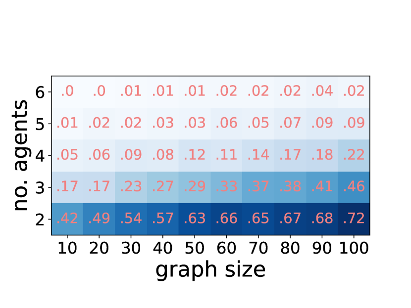
(a) EF1 and PO allocation existence.

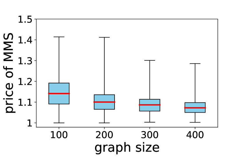
(b) Price of MMS.

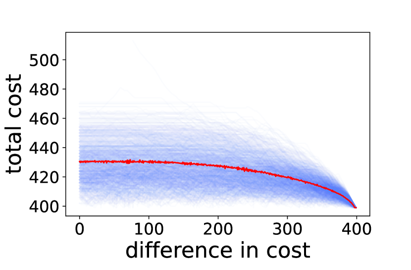
(c) Pareto frontier.

Figure 4: Figure 4(a) shows the probability that there is an EF1 and PO allocation for different number of agents and sizes of graphs. Figure 4(b) presents the boxplots with the price of fairness (MMS) for 2 agents and different graph sizes. In Figure 4(c) we analyze the trade-off between fairness and the total cost of agents in singular Pareto frontiers for 2 agents and graphs with 400 vertices.

Experiment 1. EF1 and PO allocation existence.

First, we checked how often there exists an EF1 and PO allocation. To this end, we generated trees of sizes $10,20,\dots,100$ and for each tree we run Algorithm 1 for each number of agents from 2 to 6. Based on the output, we checked the number of trees that admit an EF1 and PO allocation. As shown in Figure 4(a), the probability of finding an EF1 and PO allocation increases steadily when we increase the size of the graph, but drops sharply when we increase the number of agents. Intuitively, on larger graphs we have more flexibility in how we fairly split the vertices in a PO way. However, when there are more agents, it may still be difficult to satisfy fairness for each agent. We repeat a similar experiment for EF1 and SO as well as MMS and SO allocations in Appendix F.

Experiment 2. Price of fairness.

Next, we analyze price of fairness of MMS allocations. To this end, we generated trees of sizes $100,200,300,400$ and we run Algorithm 1 for two agents (we consider more graph sizes and also three agents in Appendix F). We computed the price of fairness as the ratio of the minimum total cost of agents in an MMS allocation to the minimum total cost in any allocation (i.e., the number of edges in a graph). Figure 4(b) illustrates that the median price is around $1.15$ for the graphs of size 100 and it steadily decreases for the larger graphs. These results suggest that as the size of the instance grows, the efficiency loss due to MMS becomes negligible in most cases (at least for a small number of agents).

Experiment 3. Pareto frontiers.

In our final experiment, we analyze the trade-off between fairness and the total cost of agents in singular Pareto frontiers. To this end, we focus on a single size of a graph, 400, and two agents. For each one of 1000 trees generated, we look at each allocation in the Pareto frontier and report the total cost of both agents on y-axis and the difference in costs of agents on x-axis. Then, we connect all such points for allocations in one Pareto frontier to form a partially transparent blue line. By superimposition of all 1000 of such blue lines, we obtain a general view on the distribution of Pareto frontiers. With the thick red line we denote the average total cost, for each difference in costs. We see that particular Pareto frontiers can behave very differently, but the general pattern is quite strong: The total cost does not vary much when the difference in costs is between 0 and 250, however it is much steeper for the larger differences. These findings imply that it is usually not effective to focus on partial fairness as the additional total cost that we incur by guarantying complete fairness instead of partial is not that big. We present similar experiment for different graph sizes and numbers of agents in Appendix F.

7 Conclusions and Future Work

We introduced a novel problem of fair distribution of delivery orders on tree graphs. We provided a comprehensive characterization of the space of instances that admit fair (EF1 or MMS) and efficient (SO or PO) allocations and—despite proving their hardness—developed an XP algorithm parameterized by the number of agents for each combination of fairness-efficiency notions.

Our work paves the way for future research on developing approximation schemes or perhaps algorithms parameterized by graph characteristics (e.g., maximum degree or diameter) in this domain. Another intriguing direction is generalizing our fair delivery framework to account for cyclic graphs, heterogeneous cost functions, or capacity constraints on delivery orders assigned to each agent.

Appendix

Appendix A Additional Related Work

Fair division of indivisible items has garnered much attention in recent years. Several notions of fairness have been explored here with EF1 [Lipton et al., 2004, Budish, 2011, Barman et al., 2018, Caragiannis et al., 2019, Barman et al., 2019] and MMS [Barman et al., 2019, Barman and Krishnamurthy, 2020, Ghodsi et al., 2018, Procaccia and Wang, 2014, Hosseini and Searns, 2021] being among the most prominent ones. An important result from this space is from Caragiannis et al. [2019] showing that an EF1 and Pareto Optimal allocation is guaranteed to exist. In our setting we find that this is no longer the case. We use the leximin optimal allocation to provide a characterisation for settings where EF1 and PO can simultaneously be satisfied. In prior work, Plaut and Roughgarden [2020] use a specific type of leximin optimal allocation to find $\mathrm{EFX}$ allocations under subadditive valuations. We also provide a characterisation of when EF1 and socially optimal (SO) allocations exist. Such an allocation would maximize the social welfare (sum of all agents’ values) and also be fair. Prior work has looked at maximizing SW over EF1 allocations [Barman et al., 2019, Benabbou et al., 2020, Caragiannis and Narang, 2022].

Submodular valuations and their subclasses have been well studied in prior work. Typically, submodular valuations require oracle access as the functions tend to be too large to be sent as an input to the algorithm. Depending on the type of oracle access, the abilities and efficiency of the algorithm changes. Submodular valuations and its subclasses have also been explored in fair division literature, especially in the context of MMS [Barman and Verma, 2021, Barman and Krishnamurthy, 2020, Ghodsi et al., 2018, Benabbou et al., 2020, Li and Vondrák, 2021, Barman and Verma, 2022]. Additionally, while the majority of the work in this space has looked at settings with goods, some recent work also looks at chores, either alone or in conjunction with goods [Aziz et al., 2022, Bhaskar et al., 2021, Caragiannis and Narang, 2022, Hosseini et al., 2022, Huang et al., 2016, Freeman et al., 2019].

Submodular costs have been studied in various algorithmic settings, be it combinatorial auctions, facility location or other graph problems like shortest cycles. Of these the only study to look at a cost model similar to ours is Svitkina and Tardos [2006] where the authors consider submodular facility costs using a rooted tree whose leaves are the facilities. The facility costs of opening a certain set of facilities was the sum of the weights of the vertices needed to be crossed from the root to reach reach these facilities from the root. While this is very similar to the cost functions in our model, it is important to note that this work has no fairness considerations, only aiming to minimise the total costs. Needless to say, this can cause a large discrepancy in the workloads of different facilities.

Fairness with Graphs

Some prior work has also looked at fair division on graphs [Bouveret et al., 2017, Bilò et al., 2022, Truszczynski and Lonc, 2020, Misra et al., 2021, Misra and Nayak, 2022]. With the exception of Misra and Nayak [2022], all other papers looked at settings where items are on a graph and each agent must receive a connected bundle. Our model does not have such a restriction. The purpose behind the prior work done in fair division on graph is to partition the graph into $n$ vertex-disjoint connected subgraphs. The value of the agents comes only from the vertices in their bundle, and does not depend on vertices outside of their bundle. In our case, the subgraphs will always intersect in the hub. Additionally, for us, the bundle that an agent receives need not form a connected subgraph. The cost depends on the distances of these vertices to the hub, which is in not allocated. Thus, agents can incur costs from having to traverse vertices that are not in their bundles. Misra and Nayak [2022] look at a setting where agents are connected by a social network and only envy those agents they have an edge to.

Work on fairness in delivery settings has been almost entirely empirical [Nair et al., 2022, Gupta et al., 2022] and no positive theoretical guarantees have been provided. The aim is typically to achieve fairness by income distribution, which differs from our approach. We look for fairness in the workload of the delivery agents, as there can be many settings where agents receive no or fixed monetary compensation for their work.

While fairness has been studied in routing problems, the aim has been to balance the amount of traffic on each edge [Kleinberg et al., 1999, Pioro, 2007]. This does not capture the type of delivery instances that we look at. Some work has also looked at ride-hailing platforms and aiming to achieve group and individual fairness in these settings [Sánchez et al., 2022, Esmaeili et al., 2022]. However, these studies are largely experimental and do not provide any theoretical guarantees. Further, these models also do not look at models with submodular costs. In fact, they use linear programs to achieve their experimental results.

There is a large body of work that looks at supply chain optimization [Geunes and Pardalos, 2006, Narahari and Srivastava, 2007, Garg et al., 2005, Biswas and Narahari, 2004, Narahari and Biswas, 2007]. The focus is to make each portion of the supply chain here more efficient. We assume that the technicalities of the supply chain are already fixed. The study of fairness in this area focuses largely on fair profit distribution [Chen et al., 2003, Yue and You, 2014, Sawik, 2015, Qiu et al., 2023].

Appendix B Graph Preliminaries

A graph is defined by a pair $G=(V,E)$, where $V$ (or $V(G)$) is a set of vertices and $E$ (or $E(G)$) is a set of (undirected) edges. A walk is a sequence of vertices $(v_{0},\dots,v_{k})$ such that every two consecutive vertices are connected by an edge. The length of a walk is the number of edges in it, so the number of vertices minus 1. A path is a walk in which all vertices are pairwise distinct. A graph is connected if there exists a walk between every pair of vertices in $V$. In a connected graph, a distance between vertex $u$ and $v$, i.e., $\mathrm{dist}(u,v)$, is the minimum length of a walk connecting $u$ and $v$.

A subgraph of graph $G$ is any graph $H=(U,M)$ such that $U\subseteq V$ and $M\subseteq E$. A subgraph is induced if for every edge $(u,v)\in E$ such that $u,v\in U$ we have $(u,v)\in M$.

A tree is a graph in which between every pair of vertices there exists exactly one path. A rooted tree is a tree with one vertex, $h\in V$, designated as a root. For every vertex $u\in V$, its ancestor is every vertex in a path from $u$ to $h$ except for $u$. For such vertices $u$ is a descendant. An ancestor (or descendant) connected by an edge is called a parent (or child). A vertex without children is called a leaf; otherwise it is internal. A subtree rooted in $u$ is an induced subgraph $T_{u}=(U,M)$ rooted in $u$, where $U$ contains $u$ and all its descendants. By a branch outgoing from $h$ we understand a set of nodes of a subtree rooted in a child of the root $h$.

Appendix C MMS and Envy-Freeness

The notion of the maximin fair share was introduced by Budish [2011], which was also the first time the notion of EF1 was explicitly defined (Lipton et al. [2004] define it implicitly). When valuations are identical, MMS allocations are guaranteed to exist, as the allocation that defines the MMS value will satisfy MMS for all agents. Unfortunately, MMS allocations need not exist when valuations are not identical. However, for additive goods, a $\nicefrac{{3}}{{4}}$-MMS is guaranteed to exist Ghodsi et al. [2018]. For additive chores, a $\nicefrac{{4}}{{3}}$-MMS allocation is guaranteed to exist [Barman and Krishnamurthy, 2020].

It is well-known that EF implies MMS for additive items, via Proportional share. However, EF1 does not imply MMS, even for identical additive valuations. In fact even the stronger notion of envy-freeness up to any item (EFX) does not imply MMS for identical valuations (EFX is a stricter notion than EF1 that requires that on the removal of any item, envy-freeness must be satisfied). Take a simple example. Let there be two agents and four goods, $g_{1}$ and $g_{2}$ both giving a value of 2, and $g_{3})$ and $g_{4}$ giving a value of 1 each. Here an MMS allocation would give both agents a value of 3. Now, the allocation $(\{g_{1},g_{2}\},\{g_{3},g_{4}\})$ is EFX (and hence, EF1) but clearly not MMS.

From Plaut and Roughgarden [2020] we know that when valuations are identical and the marginal values are positive for all goods, the leximin optimal allocation will be EFX and hence EF1. Now the leximin optimal under identical values is always MMS, hence an allocation that is both MMS and EFX always exists here. Further, Barman and Krishnamurthy [2020] give an algorithm that satisfies both EFX and $\nicefrac{{2}}{{3}}$-MMS for identical additive valuations.

Unfortunately, even EF need not imply MMS under our setting. Consider the instance and allocation depicted in Figure 5. Both agents incur a combined cost of 3, but the MMS cost is 2.

Figure 5: An example graph showing that EF does not imply MMS. The visible allocation, i.e., $(\{a,c\},\{b,d\})$, is EF but not MMS.

Appendix D Additional Material for Section 4

In this section, we present the formal proofs of several statements from Section 4.

See 3

Proof.

Observe that the sum of the costs of all agents can never be smaller than the number of edges in the graph, i.e., $|E|=m$. Indeed, since every vertex has to be serviced by some agent, each edge must appear in $G|_{A_{i}}$ for some $i\in[n]$. Moreover, if every branch outgoing from the hub is fully contained in some bundle, every edge appears in $G|_{A_{i}}$ for exactly one $i\in[n]$. Hence, in every allocation satisfying the assumption, the total costs is equal to $m$ and thus the allocation is SO.

Now, consider an allocation in which there exists a branch, $B$, and agents $i\neq j$ such that $B\cap A_{i}\neq\varnothing$ and $B\cap A_{j}\neq\varnothing$. Let $u$ be a vertex in $B$ connected to the hub, $h$. Then, edge $(h,u)$ appears in both $G|_{A_{i}}$ and $G|_{A_{j}}$. Since every other edge appears in $G|_{A_{k}}$ for at least one $k\in[n]$, we get that the total cost is greater than $m$. Thus, such an allocation is not SO. ∎

See 4

Proof.

Example 2 shows that there can exist instances where no SO allocation satisfies MMS or EF1. Now recall the proof of Theorem 1. Observe that the MMS allocations in the case when the original instance does admit a 3-Partition must also be SO. Hence, finding an MMS and SO allocation when one exists is NP-hard.

Now from Proposition 7 for any EF1 and SO allocation, $A=(A_{1},\ldots,A_{n})$, for any $i,j$, it must be that $|c(A_{i})-c(A_{j})|\leq 1$. As $\sum_{i=1}^{n}c(A_{i})=nT$, there exist $i$ s.t. $c(A_{i})<T$ if and only if there exists $i^{\prime}$ such that $c(A_{i})>T$. Thus, for such an $i$, EF1 is violated. Consequently, an EF1 and SO allocation must give cost $T$ to all agents.

Hence, an EF1 and SO allocation exists if any only if a there exists a 3-Partition. ∎

See 3

Proof.

From Proposition 3 we know that the allocation has to be a partition of whole branches outgoing from $h$. Hence, the thesis follows from the definition of MMS. ∎

See 8

Proof.

Recall the proof of Theorem 1 and Proposition 4. In the instances constructed, we can show that any PO allocation must be SO.

Let $A$ be an allocation that is not SO. Thus, there exists vertex $v_{j}^{t}$ that is visited by multiple agents. Clearly, $v_{j}^{t}$ is not a leaf. Let $v_{j}^{s_{j}}$ be serviced by agent $i$. Consider allocation $A^{\prime}$ which is identical to $A$ with the exception that $i$ services all of $v_{j}^{1},\cdots,v_{j}^{s_{j}}$. Clearly, the cost of $i$ is the same as that in $A$, but the costs of all other agents either decrease or remain the same. As multiple agents, including $i$ visit $v_{j}^{t}$, the cost of at least one agent reduces. Consequently, $A^{\prime}$ pareto dominates $A$. Thus, every PO allocation in our constructed graph must be SO.

Hence, any polynomial time algorithm to find an MMS and PO allocation or find an EF1 and PO allocation when one exists, would also find the corresponding SO allocations and solve 3-Partition. Thus, we have the proposition. ∎

Appendix E Additional Material for Section 5

In this section, we fully describe auxiliary procedure, Algorithm 2, and formally prove the correctness of Algorithm 1. We further show how it can be used to find allocations satisfying a combination of fairness and efficiency notions (or check if they exist).

We begin by introducing some additional notation. By $\Pi_{n}$ let us denote the set of all permutations of set $[n]$. For a permutation $\pi\in\Pi_{n}$ and allocation $A=(A_{1},\dots,A_{n})$, by $\pi(A)$ we understand allocation $(A_{\pi(1)},\dots,A_{\pi(n)})$, i.e., allocation where agent $i$ receives the original bundle of agent $\pi(i)$. For two partial allocations, $A=(A_{1},\dots,A_{n})$ and $B=(B_{1},\dots,B_{n})$, with disjoint set of distributed vertices, i.e., $\bigcup_{i\in[n]}A_{i}\cap\bigcup_{i\in[n]}B_{i}=\varnothing$, by $C=A\oplus B$, we understand allocation $C=(A_{1}\cup B_{1},\dots,A_{n}\cup B_{n})$. For two allocations $A$ and $B$ we write $A<_{PO}B$, when $A$ is Pareto dominated by $B$. We write $A\leq_{PO}B$, when it is weakly Pareto dominated, i.e., $c(A_{i})\geq c(B_{i})$ for every $i\in[n]$. Now, we are ready to describe auxiliary Algorithm 2 that combines two lists of allocations, $\mathcal{F}$ and $\mathcal{F}^{\prime}$.

1:  $Res=[\ ]$, empty list of allocations

2:  for  $A\in\mathcal{F},B\in\mathcal{F}^{\prime},\pi\in\Pi_{n}$ do

3:     $C=$ sort$(A\oplus\pi(B))$

4:     if there is no $D\in Res$ s.t. $C\leq_{PO}D$ then

5:        add $C$ to $Res$

6:        while there is $D\in Res$ s.t. $D<_{PO}C$ do

7:           remove $D$ from $Res$

8:        end while

9:     end if

10:  end for

11:  return  $Res$

Algorithm 2 CombineFrontiers($\mathcal{F},\mathcal{F}^{\prime}$)

Algorithm.

First, we initialize empty output list $Res$ (line 1). Then, we iterate over all possible triples $(A,B,\pi)$, where $A$ and $B$ are allocations from input lists $\mathcal{F}$ and $\mathcal{F}^{\prime}$, respectively, and $\pi$ is a permutation of agents $[n]$ (line 2). For each such triple, we consider allocation $C=\mathrm{sort}(A\oplus\pi(B))$, i.e., the allocations in which agent $i$, receives bundle $A_{i}\cup B_{\pi(i)}$, sorted in non-increasing cost order. In the next step, we check if there exists an allocation $D$ in $Res$ that weakly Pareto dominates $C$ (line 4). If this is the case, we disregard $C$ and move to the next triple. If this is not the case, then we add allocation $C$ to the list $Res$ (line 5) and remove all allocations $D$ from $Res$ that are Pareto dominated by $C$ (lines 6–8). We note that operations in lines 4–8 can be performed more efficiently if we keep allocations in $Res$ in a specific ordering, but since it is not necessary for our results, we do not go into details for the sake of simplicity. After considering all pairs and permutations, we return list $Res$ (line 11).

See 5

Proof.

Let us start by showing that the output is a Pareto frontier, which we will prove by induction on the number of edges in a graph. If there is only one edge, the graph consists of the hub, $h$, and one vertex connected to it, say $u$. Then, there is only one possible allocation (up to a permutation of agents), namely, $(\{u\},\varnothing,\dots,\varnothing)$, and it is PO. Observe that this is also the only allocation returned by our algorithm for such a graph. Hence, the inductive basis holds.

Now, assume that our algorithm outputs a Pareto frontier for every instance, in which the number of edges is smaller or equal to $M$ for some $M\in\mathbb{N}$ and consider an instance $\langle[n],G,h\rangle$ with $M+1$ edges. Take arbitrary PO allocation $A$. We will show that in the output of Algorithm 1 for this instance, $\mathcal{F}$, there exists allocation $B$ such that $c(A_{i})=c(B_{\pi(i)})$ for some permutation $\pi\in\Pi_{n}$.

If $h$ has only one child, $u$, then observe that every agent that services some vertex in $A$ has to visit $u$. Also, the agent that services $u$ services also other vertices (otherwise giving $u$ to an agent that services some other vertex would be a Pareto improvement). Hence, partial allocation $A^{\prime}$ obtained from $A$ by removing $u$ is still PO and the cost of each agent is the same in both allocations. Observe that $A^{\prime}$ is also a PO allocation in instance $\langle[n],T_{u},u\rangle$. Let $\mathcal{F}^{\prime}$ be the output of Algorithm 1 for instance $\langle[n],T_{u},u\rangle$. Then, since $T_{u}$ has $M$ edges, from inductive assumption we know that there exists $B^{\prime}\in\mathcal{F}^{\prime}$ and $\pi\in\Pi_{n}$ such that $c(A^{\prime}_{i})=c(B^{\prime}_{\pi(i)})$, for every $i\in[n]$. Then, let $B$ be an allocation obtained from $B^{\prime}$ by adding $u$ to the bundle of agent $1$. Since we sort allocation so that consecutive agents have nonincreasing costs, we know that $B^{\prime}_{1}\neq\varnothing$. Hence, cost of each agent in $B$ is the same as in $B^{\prime}$. Hence, $c(A_{i})=c(A^{\prime}_{i})=c(B^{\prime}_{\pi(i)})=c(B_{\pi(i)})$. Since $B$ is in the output of the algorithm, the induction thesis holds.

Now, assume that $h$ has more than one child. Let us denote them as $u^{1},\dots,u^{k}$ and by $U^{1},\dots,U^{k}$ let us denote the respective branches outgoing from $h$. Let $A^{1},\dots,A^{k}$ be partial allocations obtained from $A$ by restricting $A$ to one branch from $U^{1},\dots,U^{k}$, respectively (i.e., removing all vertices not in the branch from all of the bundles). Observe that since $A$ is PO, each allocation $A^{1},\dots,A^{k}$ is also PO (otherwise a Pareto improvement in $A^{j}$ for some $j\in[k]$ would be a Pareto improvement also in $A$). With the same reasoning as in the previous paragraph, by line 6 of Algorithm 1 in the iteration of the loop for each child $u^{j}$, list $\mathcal{F}^{\prime}$ contains an allocation $B^{j}$ such that $c(A^{j}_{i})=c(B^{j}_{\pi^{j}(i)})$ for some $\pi^{j}\in\Pi_{n}$ and every $i\in[n]$. Now, when we combine $\mathcal{F}$ with $\mathcal{F}^{\prime}$ we consider all possible combinations of allocations in $\mathcal{F}$ and $\mathcal{F}^{\prime}$ along with all possible permutations of agents. Hence, in the output of the algorithm, there will be allocation $B$ and permutation $\pi\in\Pi_{n}$ such that $B_{\pi(i)}=B^{1}_{\pi^{1}(i)}\cup\dots\cup B^{k}_{\pi^{k}(i)}$ for every $i\in[n]$, unless there is some allocation $D$ that weakly Pareto dominates $B$. Since $A^{1},\dots,A^{k}$ are partial allocations of separate branches and $B^{1},\dots,B^{k}$ as well, we have

$$c(B_{\pi(i)})=\textstyle\sum_{j\in[k]}c(B^{j}_{\pi^{j}(i)})=\textstyle\sum_{j\in[k]}c(A^{j}_{i})=c(A_{i}),$$

for every $i\in[n]$. Hence, $B$ is PO. Thus, if there is $D$ that weakly Pareto dominates $B$, then $c(D_{i})=c(B_{i})$ for every $i\in[n]$. Either way, there exists an allocation in $\mathcal{F}$ that for corresponding agents gives the same costs as allocation $A$. Therefore, $\mathcal{F}$ is a Pareto frontier, which concludes the induction proof.

In the rest of the proof, let us focus on showing that the running time of Algorithm 1 is $O((n+2)!m^{3n+1})$. To this end, recall that in lines 2–10 of auxiliary Algorithm 2 we consider all triples $(A,B,\pi)$, where $A$ is an allocation in $\mathcal{F}$, $B$ an allocation in $\mathcal{F}^{\prime}$, and $\pi$ a permutation in $\Pi_{n}$. Since the cost of an agent is an integer between $0$ and $m$ and at any moment we cannot have two allocation with the same cost for every agent in $\mathcal{F}$ or $\mathcal{F}^{\prime}$ (because one is weakly Pareto dominated by the other), the sizes of $\mathcal{F}$ and $\mathcal{F}^{\prime}$ are bounded by $(m+1)^{n}$. Hence, the loop in lines 2–10, will have at most $n!(m+1)^{2n}$ iterations. For each triple, we have to sort the resulting allocation, which can take time $n\log(n)$. Moreover, we may need to check whether resulting allocation $C$ Pareto dominates or is Pareto dominated by all of the allocations already kept in $Res$. The size of $Res$ is also bounded by $(m+1)^{n}$ and checking Pareto domination can be done in time $n$. All in all, the running time of Algorithm 2 is in $O((n+2)!m^{3n})$. Finally, observe that in Algorithm 1 we call Algorithm 2 less than $m$ times, thus final running time is in $O((n+2)!m^{3n+1})$. ∎

Now, let us show how we can use Algorithm 1 to find allocation satisfying certain fairness and efficiency requirements (or decide if they exist).

See 6

Proof.

Let us split the proof into four lemmas devoted to each combination of fairness and efficiency notions. We start with MMS and PO allocations.

Lemma 1.

There exists an XP algorithm parameterized by $n$ that for every delivery instance $\langle[n],G,h\rangle$ finds an MMS and PO allocation.

Proof.

Observe that the allocation in a Pareto frontier that leximin dominates all other allocations in the frontier is a leximin optimal allocation. Since Algorithm 1 returns a Pareto frontier, and Pareto frontier contains at most $O(m^{n})$ allocations, we can find such an allocationin XP time by Theorem 5. Therefore, the lemma follows from Proposition 6. ∎

Next, let us move to EF1 and PO allocations.

Lemma 2.

There exists an XP algorithm parameterized by $n$ that for every delivery instance $\langle[n],G,h\rangle$ decides if there exists an EF1 and PO allocation and finds it if it exists.

Proof.

From the proof of Theorem 4 and Proposition 7 we know that an EF1 and PO allocation is leximin optimal and the pairwise differences in the costs of agents are at most 1. Observe that it is an equivalence, i.e., a leximin optimal allocation in which the pairwise differences in the costs of agents are at most 1 is EF1 and PO (PO because of leximin optimality, and EF1 because for every agent there exists a vertex that removed from a bundle of this agent reduces the cost by at least 1). By Lemma 1, we can find a leximin optimal allocation in XP time with respect to $n$. Therefore, it remains to check if the pairwise differences in the costs of agents are at most 1. If it is true, then we know that this allocation is EF1 and PO. Otherwise, we know there is no EF1 and PO allocation. ∎

Now, let us consider MMS and SO allocations.

Lemma 3.

There exists an XP algorithm parameterized by $n$ that for every delivery instance $\langle[n],G,h\rangle$ decides if there exists an MMS and SO allocation and finds it if it exists.

Proof.

For MMS and SO, observe that an SO allocation is also necessarily a PO allocation. Having Pareto frontier from Theorem 5 and MMS value from Lemma 1, we can simply check all allocation in the frontier if they satisfy MMS and SO. ∎

Finally, we focus on EF1 and SO allocations.

Lemma 4.

There exists an XP algorithm parameterized by $n$ that for every delivery instance $\langle[n],G,h\rangle$ decides if there exists an EF1 and SO allocation and finds it if it exists.

Proof.

For EF1 and SO, observe that Theorem 4 also implies that EF1 and SO allocation is MMS. From Lemma 3 we know that we can find all MMS and SO allocations in Pareto frontier in XP time with respect to $n$. Hence, we can check if any one of them satisfies also EF1 and this will give us the solution. ∎

From Lemmas 1, 2, 3 and 4 we obtain the thesis. ∎

Appendix F Additional Experiments

In this section, we present additional experiments not included in Section 6. As in Section 6, for every experiment and every graph size we generated 1,000 trees.

Running Time of Algorithm 1

We run Algorithm 1 for graphs of sizes $10,20,\dots,100$ and every number of agents from $2$ to $6$. The running times are reported in Figure 6(a) (the running time for $2$ agents is not reported as it would be indistinguishable from the running times for 3 agents in the picture). The power in the running time of our algorithm for $n=6$ agents is significant, hence the sharp increase in the running time with growing graph size in this case.

Fair and SO Allocation Existence

In order to check how often there exist EF1 and SO allocations as well as MMS and SO ones, we generated graphs of sizes $10,20,\dots,100$ and run Algorithm 1 for all numbers of agents from 2 to 6 (identical setup to this for EF1 and PO allocations presented in Section 6, Experiment 1).

The results for EF1 and SO allocations are presented in Figure 6(b). There, we see a sharp decrease in probability with the increase in either number of agents or the size of a graph. For the former it is clear, as with larger number of agents it is difficult to be fair to all of them. For the size of a graph, recall Corollary 1 in which we have shown that EF1 and SO allocation exists only if the hub is in the center of a tree. Moreover, the tree always contains one or two vertices. Hence, with the increase in the size, the probability that the hub will be in the center decreases.

The results for MMS and SO allocations are presented in Figure 6(b). As can be seen in the picture, the probability does not really vary much between different numbers of agents (especially for small graphs). A plausible explanation for that phenomenon is that for MMS we only have to care to not be unfair to the worst off agent. If we have a small graph and a lot of agents, then probably some of them will not be assigned to any vertex either way. However, the number of such agents does not impact whether an allocation is MMS or not. Hence the visible effect.

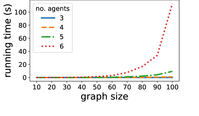
(a) Running time.

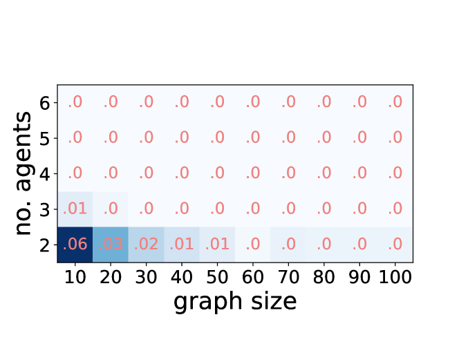
(b) EF1 and SO allocation existence.

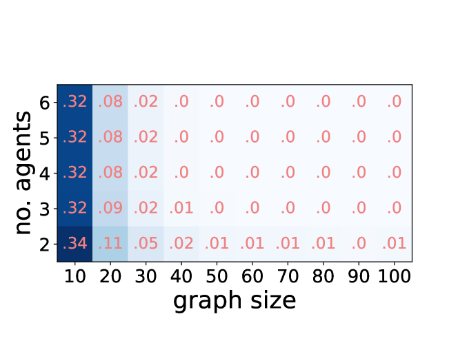
(c) MMS and SO allocation existence.

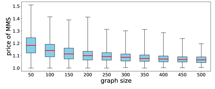
(a) Price of MMS for 2 agents.

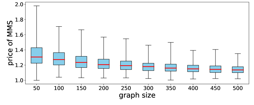
(b) Price of MMS for 3 agents.

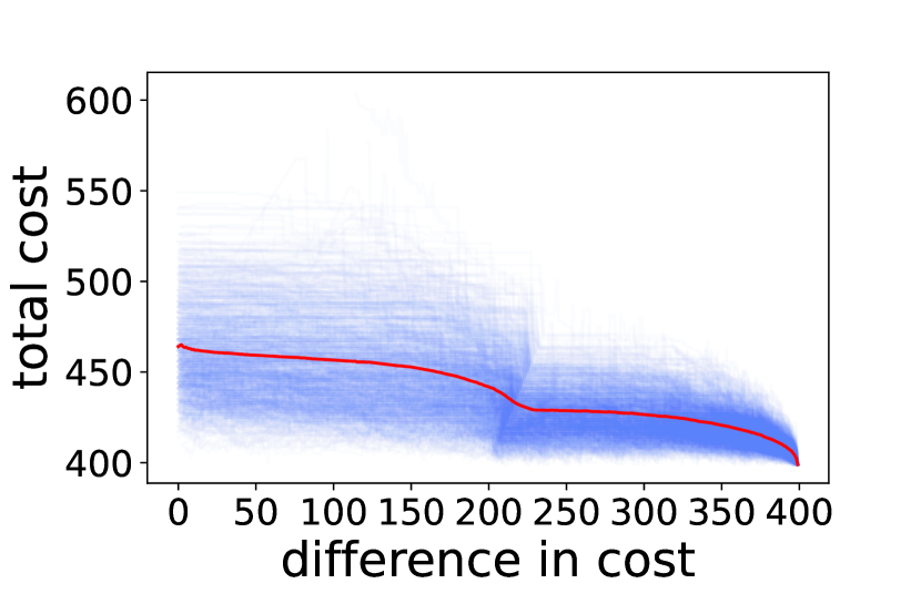
(a) Pareto frontier (3,400).

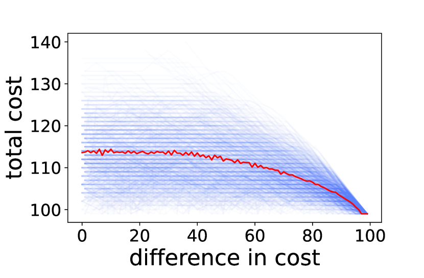
(b) Pareto frontier (2,100).

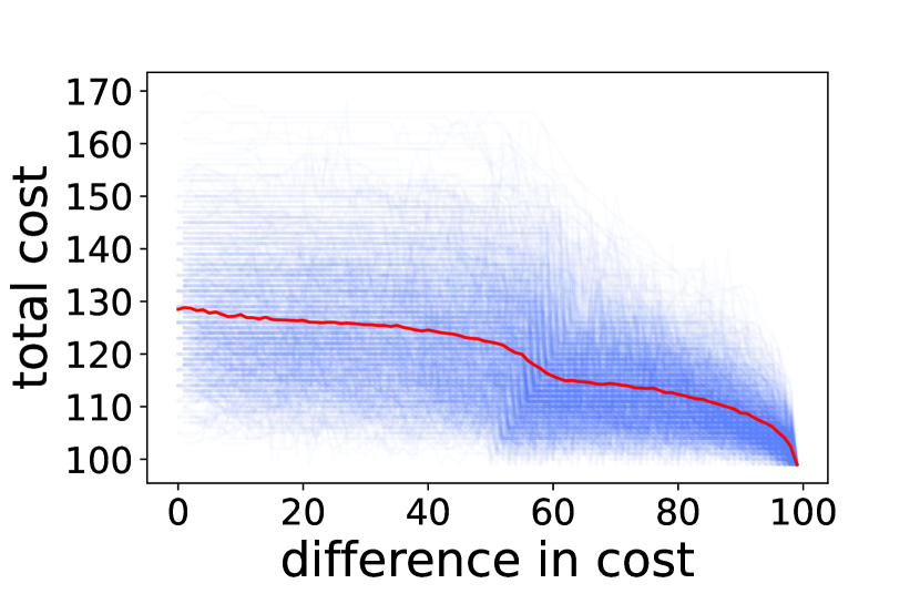
(c) Pareto frontier (3,100).

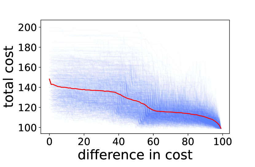
(d) Pareto frontier (4,100).

Figure 8: The results of our additional experiments. Figure 6(a) shows the average running time of Algorithm 1. Figures 6(c) and 6(b) present the probability of existence of EF1 and SO as well as MMS and SO allocations. Figures 7(a) and 7(b) depict boxplots of the distribution of price of MMS for different sizes of graphs and 2 or 3 agents, respectively. Finally, in Figures 8(a), 8(b), 8(c) and 8(d) with caption “Pareto frontier ($n$, $m$)”, we see distribution of Pareto frontiers for $n$ agents and graphs of size $m$.

Price of Fairness

We repeat our experiment with price of fairness (Experiment 2) for graphs of sizes $50,100,150,\dots,500$ and 2 and 3 agents. For each instance we computed the price of fairness as the ratio of the minimum total cost of agents in an MMS allocation to the minimum total cost in any allocation (i.e., the number of edges in a graph). The results are reported in boxplots in Figures 7(a) and 7(b). As can be seen, the median price gradually decreases with the increase of the graph size. This is aligned with our observations made in Section 6.

Pareto frontier

Finally, we repeat the experiment that analyzes the trade-off between fairness and the total cost of agents in singular Pareto frontiers (Experiment 3). For each one of 1000 trees generated, we look at each allocation in the Pareto frontier and report the total cost of all agents on y-axis and the maximal difference in costs between a pair of agents on x-axis. Next, if there are several allocations with the same maximal difference in costs between a pair of agents we keep only the one with the minimal total cost. Then, we connect all of the points for allocations in one Pareto frontier to form a partially transparent blue line. By superimposition of all 1000 of such blue lines, we obtain a general view on the distribution of Pareto frontiers. With the thick red line we denote the average total cost, for each difference in costs. In Section 6, we have analyzed graphs of size 400 and 2 agents. Here, we present also the analysis of the same size with 3 agents, and graphs of size 100 with 2, 3, and 4 agents.

The plot for the size 100 and 2 agents looks very similar to the one presented in Figure 4(c). Again, we can say, that the total cost for agents increases sharply when we decrease the difference in costs of agents from 400, but the further we go, this increase is slower.

For 3 agents and both graph sizes, the plots look similar to these for 2 agents in their right-hand side part. However, a little to the right from the middle of the picture, we see a sudden sharp increase in the total cost that later also flattens. We offer the following interpretation of this fact: in the rightmost part of the plot we begin with an allocation where the first agent is serving all of the nodes, which gives us the minimal total cost, but also the maximal difference between the costs of two agents. Then, when we want to decrease the difference, we have to take some of the vertices served by the first agent, and give it to some other agent. However, as only the maximal difference between the agents is important to us, we can, for now, split the vertices only between the first two agents, which is easier (i.e., results in a smaller total cost). However, when we reach the difference in cost that is around the half of the graph size, this is no longer possible. To decrease the difference further, we have to start assigning vertices to the third agent, which brings additional cost. Thus, the increase in the total cost in the left-hand side half of the plot.

The situation for 4 agents is similar to this for 3 agents, but here after the first increase in a bit more than a half of the plot, where we start assigning vertices to the third agent, we see a second increase in a bit more than a third of the plot, where we start assigning vertices to the forth agent.

References

- Aziz et al. [2022] Haris Aziz, Ioannis Caragiannis, Ayumi Igarashi, and Toby Walsh. Fair allocation of indivisible goods and chores. Autonomous Agents and Multi-Agent Systems, 36(1):1–21, 2022.
- Barman and Krishnamurthy [2020] Siddharth Barman and Sanath Kumar Krishnamurthy. Approximation algorithms for maximin fair division. ACM Transactions on Economics and Computation (TEAC), 8(1):1–28, 2020.
- Barman and Verma [2021] Siddharth Barman and Paritosh Verma. Existence and computation of maximin fair allocations under matroid-rank valuations. In Proceedings of the 20th International Conference on Autonomous Agents and MultiAgent Systems, pages 169–177, 2021.
- Barman and Verma [2022] Siddharth Barman and Paritosh Verma. Truthful and fair mechanisms for matroid-rank valuations. In Proceedings of the AAAI Conference on Artificial Intelligence, volume 36, pages 4801–4808, 2022.
- Barman et al. [2018] Siddharth Barman, Sanath Kumar Krishnamurthy, and Rohit Vaish. Finding fair and efficient allocations. In Proceedings of the 2018 ACM Conference on Economics and Computation, pages 557–574, 2018.
- Barman et al. [2019] Siddharth Barman, Ganesh Ghalme, Shweta Jain, Pooja Kulkarni, and Shivika Narang. Fair division of indivisible goods among strategic agents. 18th International Conference on Autonomous Agents and MultiAgent Systems, pages 1811–1813, 2019.
- Benabbou et al. [2020] Nawal Benabbou, Mithun Chakraborty, Ayumi Igarashi, and Yair Zick. Finding fair and efficient allocations when valuations don’t add up. Symposium on Algorithmic Game Theory, pages 32–46, 2020.
- Bhaskar et al. [2021] Umang Bhaskar, AR Sricharan, and Rohit Vaish. On approximate envy-freeness for indivisible chores and mixed resources. In Approximation, Randomization, and Combinatorial Optimization. Algorithms and Techniques (APPROX/RANDOM 2021). Schloss Dagstuhl-Leibniz-Zentrum für Informatik, 2021.
- Bilò et al. [2022] Vittorio Bilò, Ioannis Caragiannis, Michele Flammini, Ayumi Igarashi, Gianpiero Monaco, Dominik Peters, Cosimo Vinci, and William S Zwicker. Almost envy-free allocations with connected bundles. Games and Economic Behavior, 131:197–221, 2022.
- Biswas and Narahari [2004] Shantanu Biswas and Y Narahari. Object oriented modeling and decision support for supply chains. European Journal of Operational Research, 153(3):704–726, 2004.
- Bouveret et al. [2017] Sylvain Bouveret, Katarína Cechlárová, Edith Elkind, Ayumi Igarashi, and Dominik Peters. Fair division of a graph. Proceedings of the Twenty-Sixth International Joint Conference on Artificial Intelligence (IJCAI-17), 2017.
- Budish [2011] Eric Budish. The combinatorial assignment problem: Approximate competitive equilibrium from equal incomes. Journal of Political Economy, 119(6):1061–1103, 2011.
- Caragiannis and Narang [2022] Ioannis Caragiannis and Shivika Narang. Repeatedly matching items to agents fairly and efficiently. arXiv preprint arXiv:2207.01589, 2022.
- Caragiannis et al. [2019] Ioannis Caragiannis, David Kurokawa, Hervé Moulin, Ariel D Procaccia, Nisarg Shah, and Junxing Wang. The unreasonable fairness of maximum nash welfare. ACM Transactions on Economics and Computation (TEAC), 7(3):1–32, 2019.
- Chen et al. [2003] Cheng-Liang Chen, Bin-Wei Wang, and Wen-Cheng Lee. Multiobjective optimization for a multienterprise supply chain network. Industrial & Engineering Chemistry Research, 42(9):1879–1889, 2003.
- Chen and Liu [2020] Xingyu Chen and Zijie Liu. The fairness of leximin in allocation of indivisible chores. arXiv preprint arXiv:2005.04864, 2020.
- Ebadian et al. [2021] Soroush Ebadian, Dominik Peters, and Nisarg Shah. How to fairly allocate easy and difficult chores. arXiv preprint arXiv:2110.11285, 2021.
- Esmaeili et al. [2022] Seyed A Esmaeili, Sharmila Duppala, Vedant Nanda, Aravind Srinivasan, and John P Dickerson. Rawlsian fairness in online bipartite matching: Two-sided, group, and individual. arXiv preprint arXiv:2201.06021, 2022.
- Freeman et al. [2019] Rupert Freeman, Sujoy Sikdar, Rohit Vaish, and Lirong Xia. Equitable allocations of indivisible goods. arXiv preprint arXiv:1905.10656, 2019.
- Garg et al. [2005] Dinesh Garg, Yadati Narahari, Earnest Foster, Devadatta Kulkarni, and Jeffrey D Tew. A groves mechanism approach to decentralized design of supply chains. In Seventh IEEE International Conference on E-Commerce Technology (CEC’05), pages 330–337. IEEE, 2005.
- Geunes and Pardalos [2006] Joseph Geunes and Panos M Pardalos. Supply chain optimization, volume 98. Springer Science & Business Media, 2006.
- Ghodsi et al. [2018] Mohammad Ghodsi, MohammadTaghi HajiAghayi, Masoud Seddighin, Saeed Seddighin, and Hadi Yami. Fair allocation of indivisible goods: Improvements and generalizations. In Proceedings of the 2018 ACM Conference on Economics and Computation, pages 539–556, 2018.
- Goldman [1971] Alan J Goldman. Optimal center location in simple networks. Transportation science, 5(2):212–221, 1971.
- Gupta et al. [2022] Anjali Gupta, Rahul Yadav, Ashish Nair, Abhijnan Chakraborty, Sayan Ranu, and Amitabha Bagchi. Fairfoody: Bringing in fairness in food delivery. In Proceedings of the AAAI Conference on Artificial Intelligence, volume 36, pages 11900–11907, 2022.
- Hagberg et al. [2008] Aric Hagberg, Pieter Swart, and Daniel S Chult. Exploring network structure, dynamics, and function using networkx. Technical report, Los Alamos National Lab.(LANL), Los Alamos, NM (United States), 2008.
- Hosseini and Searns [2021] Hadi Hosseini and Andrew Searns. Guaranteeing maximin shares: Some agents left behind. In Proceedings of the 30th International Joint Conference on Artificial Intelligence, 2021.
- Hosseini et al. [2022] Hadi Hosseini, Andrew Searns, and Erel Segal-Halevi. Ordinal maximin share approximation for goods. Journal of Artificial Intelligence Research, 74:353–391, 2022.
- Hosseini et al. [2023] Hadi Hosseini, Sujoy Sikdar, Rohit Vaish, and Lirong Xia. Fairly dividing mixtures of goods and chores under lexicographic preferences. In Proceedings of the 22nd International Conference on Autonomous Agents and MultiAgent Systems, 2023. forthcoming.
- Huang et al. [2016] Chien-Chung Huang, Telikepalli Kavitha, Kurt Mehlhorn, and Dimitrios Michail. Fair matchings and related problems. Algorithmica, 74(3):1184–1203, 2016.
- Huang and Lu [2021] Xin Huang and Pinyan Lu. An algorithmic framework for approximating maximin share allocation of chores. In Proceedings of the 22nd ACM Conference on Economics and Computation, pages 630–631, 2021.
- Johnson and Garey [1979] David S Johnson and Michael R Garey. Computers and intractability: A guide to the theory of NP-completeness. WH Freeman, 1979.
- Kleinberg et al. [1999] Jon Kleinberg, Yuval Rabani, and Éva Tardos. Fairness in routing and load balancing. In 40th Annual Symposium on Foundations of Computer Science (Cat. No. 99CB37039), pages 568–578. IEEE, 1999.
- Li and Vondrák [2021] Wenzheng Li and Jan Vondrák. Estimating the nash social welfare for coverage and other submodular valuations. In Proceedings of the 2021 ACM-SIAM Symposium on Discrete Algorithms (SODA), pages 1119–1130. SIAM, 2021.
- Lipton et al. [2004] Richard J. Lipton, Evangelos Markakis, Elchanan Mossel, and Amin Saberi. On Approximately Fair Allocations of Indivisible Goods. In Proceedings 5th ACM Conference on Electronic Commerce (EC), New York, NY, USA, pages 125–131. ACM, 2004. URL https://doi.org/10.1145/988772.988792.
- Misra and Nayak [2022] Neeldhara Misra and Debanuj Nayak. On fair division with binary valuations respecting social networks. In Conference on Algorithms and Discrete Applied Mathematics, pages 265–278. Springer, 2022.
- Misra et al. [2021] Neeldhara Misra, Chinmay Sonar, PR Vaidyanathan, and Rohit Vaish. Equitable division of a path. arXiv preprint arXiv:2101.09794, 2021.
- Nair et al. [2022] Ashish Nair, Rahul Yadav, Anjali Gupta, Abhijnan Chakraborty, Sayan Ranu, and Amitabha Bagchi. Gigs with guarantees: Achieving fair wage for food delivery workers. arXiv preprint arXiv:2205.03530, 2022.
- Narahari and Biswas [2007] Y Narahari and Shantanu Biswas. Performance measures and performance models for supply chain decision making. Measuring supply chain performance, 2007.
- Narahari and Srivastava [2007] Y Narahari and Nikesh Kumar Srivastava. A bayesian incentive compatible mechanism for decentralized supply chain formation. In The 9th IEEE International Conference on E-Commerce Technology and The 4th IEEE International Conference on Enterprise Computing, E-Commerce and E-Services (CEC-EEE 2007), pages 315–322. IEEE, 2007.
- O’Dwyer and Timonen [2009] Ciara O’Dwyer and Virpi Timonen. Doomed to extinction? the nature and future of volunteering for meals-on-wheels services. VOLUNTAS: International Journal of Voluntary and Nonprofit Organizations, 20(1):35–49, 2009.
- Pioro [2007] Michal Pioro. Fair routing and related optimization problems. In 15th International Conference on Advanced Computing and Communications (ADCOM 2007), pages 229–235. IEEE, 2007.
- Plaut and Roughgarden [2020] Benjamin Plaut and Tim Roughgarden. Almost envy-freeness with general valuations. SIAM Journal on Discrete Mathematics, 34(2):1039–1068, 2020.
- Procaccia and Wang [2014] Ariel D Procaccia and Junxing Wang. Fair enough: Guaranteeing approximate maximin shares. In Proceedings of the fifteenth ACM conference on Economics and computation, pages 675–692, 2014.
- Prüfer [1918] Heinz Prüfer. Neuer beweis eines satzes über permutationen. Archiv fur Mathematik und Physik, 27, 1918.
- Qiu et al. [2023] Rui Qiu, Qi Liao, Renfu Tu, Yingqi Jiao, An Yang, Zhichao Guo, and Yongtu Liang. Pipeline pricing and logistics planning in the refined product supply chain based on fair profit distribution. Computers & Industrial Engineering, 175:108840, 2023.
- Sánchez et al. [2022] Aitor López Sánchez, Marin Lujak, Frederic Semet, and Holger Billhardt. On balancing fairness and efficiency in routing of cooperative vehicle fleets. In Twelfth International Workshop on Agents in Traffic and Transportation co-located with the 31st International Joint Conference on Artificial Intelligence and the 25th European Conference on Artificial Intelligence (IJCAI-ECAI 2022), volume 3173, 2022.
- Sawik [2015] Tadeusz Sawik. On the fair optimization of cost and customer service level in a supply chain under disruption risks. Omega, 53:58–66, 2015.
- Skibski [2023] Oskar Skibski. Closeness centrality via the condorcet principle. Social Networks, 74:13–18, 2023.
- Svitkina and Tardos [2006] Zoya Svitkina and Éva Tardos. Facility location with hierarchical facility costs. In SODA, volume 6, pages 153–161, 2006.
- Toth and Vigo [2002] Paolo Toth and Daniele Vigo. An overview of vehicle routing problems. The vehicle routing problem, pages 1–26, 2002.
- Truszczynski and Lonc [2020] Miroslaw Truszczynski and Zbigniew Lonc. Maximin share allocations on cycles. Journal of Artificial Intelligence Research, 69:613–655, 2020.
- Yue and You [2014] Dajun Yue and Fengqi You. Fair profit allocation in supply chain optimization with transfer price and revenue sharing: Minlp model and algorithm for cellulosic biofuel supply chains. AIChE Journal, 60(9):3211–3229, 2014.