Hedonic Prices and Quality Adjusted Price Indices Powered by AI

Abstract.

Accurate, real-time measurements of price index changes using electronic records are essential for tracking inflation and productivity in today’s economic environment. We develop empirical hedonic models that can process large amounts of unstructured product data (text, images, prices, quantities) and output accurate hedonic price estimates and derived indices. To accomplish this, we generate abstract product attributes, or “features,” from text descriptions and images using deep neural networks, and then use these attributes to estimate the hedonic price function. Specifically, we convert textual information about the product to numeric features using large language models based on transformers, trained or fine-tuned using product descriptions, and convert the product image to numeric features using a residual network model. To produce the estimated hedonic price function, we again use a multi-task neural network trained to predict a product’s price in all time periods simultaneously. To demonstrate the performance of this approach, we apply the models to Amazon’s data for first-party apparel sales and estimate hedonic prices. The resulting models have high predictive accuracy, with $R^{2}$ ranging from $80\%$ to $90\%$. Finally, we construct the AI-based hedonic Fisher price index, chained at the year-over-year frequency. We contrast the index with the CPI and other electronic indices.

Key Words: Hedonic Prices, Price Index, Transformers, Deep Learning, Artificial Intelligence

1. Introduction

Economists have developed price index methods to measure how consumers are affected by price changes in the economic environment. Some of the most commonly used are price indices are the Laspeyres or Paasche indices. These measure changes in the cost of a standardized basket of products between two periods, holding the basket to be equal to the set of products purchased in the initial period (Laspeyres) or the final period (Paasche). The two are often combined into what is known as the ideal or the Fisher price index. The Fisher Price Index (FPI) is known to provide an accurate approximation for the true cost of living when the change in prices is small.

A common problem with these indices is product entry and exit, where the previous period’s prices are not available for new products and vice-versa. Hence, economists often compute so-called ‘matched indices’—indices restricted to the set of products that are bought and sold in both periods. However, this approach is subject to selection bias, as products exiting the marketplace may resemble well those that remain; this problem is especially dire when products turn over quickly. To overcome this bias, economists often use high-frequency chaining combined with compounding, for example, computing the price indices over monthly frequency and then compounding monthly inflation rates to get yearly rates. This approach does ameliorate the turnover problem provided that the rate of turnover is not high from month to month. Still, it can suffer from the so-called chain-drift bias – a high measurement bias in price level arising due to geometric compounding of errors over many steps.

Hedonic price models were introduced by Court (1939) and Griliches (1961); these models postulate that prices of differentiated products are determined by the market value of each product’s constituent characteristics. Court and Griliches suggested measuring inflation/deflation by modeling how hedonic prices change while holding product characteristics fixed. Further, one can compute hedonic prices for baskets of goods at any time point because such prices are determined only by product characteristics and use these in the Fisher price index and other price index formulas. This gives rise to the hedonic price indices, which have been employed both in academic research and by statistical agencies (e.g., Wasshausen and Moulton (2006); Office of National Statistics (2020)).

The resulting hedonic price indices are sometimes called quality-adjusted price indices because, in price index calculations, we implicitly fix the set of characteristics (”qualities”) of a basket in a reference period and compute the ratio of costs of the basket in the comparison period and in the reference period. The ability to compute hedonic prices at any time point for any product allows us to address the entry/exit problem and also reduce chain-drift biases by making ”long” or ”low-frequency” comparisons (year-to-year, for example). The success of this approach depends on both the ability of the hedonic price models to approximate real-world prices and on our ability to estimate the hedonic price function from the available data.

Provided that hedonic price models are good approximations of the real world, theory suggests that we can learn hedonic price functions by estimating regression functions that explain observed prices in terms of product characteristics $X_{j}$. In traditional empirical hedonic models, the construction of $X_{j}$ is performed using human expertise, and statistical agencies perform the data collection through extensive field surveys and interviews.

In this paper, we develop an alternative approach to building hedonic models. Our method is based on the use of electronic data and tools from AI to collect data in real-time and to generate product characteristics $X_{j}$ in an automated way, to reconstruct the price of any product accurately. The resulting approach is highly scalable and has very low cost compared to the traditional approach. Therefore, we view our approach as a potentially useful complement to the traditional methodology for measuring price-level changes.

Let us illustrate the problem we are solving as follows. In Figure 1, we show the product characteristics observable by the customer, where we see the product title, product text description, and images for the product. Our goal is to represent this information using a numerical vector $X_{j}$ of moderately high dimension (in our case, it has 2000 entries), which can be used to predict prices accurately. Moreover, the representation needs to be algorithmic and scalable.

The success of this approach depends on the existence of parsimonious structures behind images and text. Traditionally, analysts relied on human experts to represent the key features of products and find a low dimensional numerical representation $X_{j}$. Successful experts did produce low-dimensional representations for certain groups of products, which proved to be successful in building hedonic models (e.g., Pakes (2003) reports very high accuracy for predicting computer prices). However, this approach does not scale well to many types of products and is prone to judgment biases. These issues raise important questions: When human experts succeed, what is the underlying reason? Can we replicate this success with artificial intelligence, and can these methods deliver scalable inference?

Arguably, humans can easily summarize the red dress image in Figure 1 and the accompanying text, even though the original representation of this information lives in an extremely high-dimensional space (i.e. millions of dimensions). Indeed, the image consists of nearly one million pixels (three layers of 640 x 480 pixels encoding the blue, red, and green color channels), words belong to a dictionary whose dimension is in the tens of thousands and sentences live in much higher-dimensional space. However, we believe that the images and sentences can be accurately represented in a much lower-dimensional space, a phenomenon we call ”structured sparsity.” Human intelligence can exploit this structured sparsity to process information effectively—perhaps using the geometry of shapes in images, the relative simplicity of color schemes and shade patterns, the similarity of many words in the dictionary, and the context-specific meaning of words. The field of artificial intelligence (AI) developed neural networks to mimic human intelligence in many information-processing tasks. These models do create parsimonious structures from high-dimensional inputs and often surpass human ability in such tasks. Going forward, we will employ state-of-the-art solutions from AI to the problem of hedonic modeling.

Figure 1. An example of product characteristics for a product sold in the Amazon store

In this work we extract relevant product attributes or features from text and images using cutting-edge deep learning models, then use these features to estimate the hedonic price function. Specifically, we convert text information about the product to numeric features (embeddings) using the BERT deep learning model (Devlin et al., 2018), which has been fine-tuned on Amazon’s product descriptions and further (very lightly) fine-tuned for price prediction. We similarly use a pre-trained ResNet50 model (He et al., 2016) to produce embeddings for product images. For context, these models were initially trained to comprehend text and images in tasks unrelated to predicting prices (e.g., image classification or predicting a missing word in a sentence). We then take the internal numeric representation generated by each model as an information-rich, parsimonious embedding of the input. With these embeddings, we then estimate the hedonic price function using a multi-task neural network. In particular, our networks are trained to predict prices simultaneously in all periods.

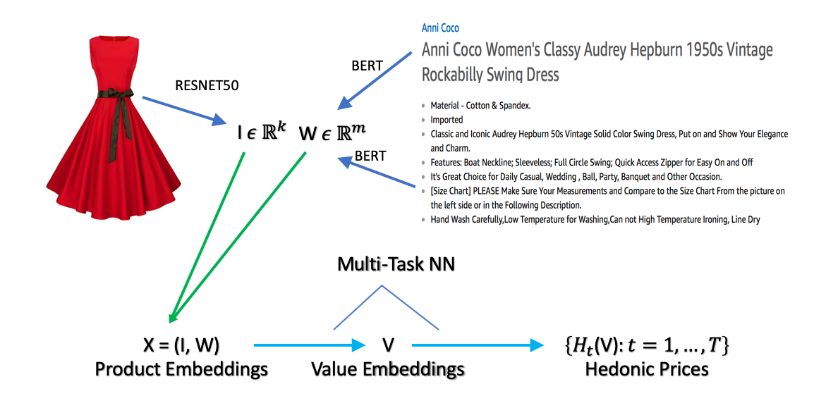
Figure 2. Our method for generating hedonic price: The input consists of images and unstructured text data. The first step of the process creates the moderately high-dimensional numerical embeddings $I$ and $W$ for images and text data via state-of-the-art deep learning methods, such as ResNet50 and BERT. The second step of the process takes input $X=(I,W)$ and creates predictions for hedonic prices $H_{t}(X)$ using deep learning methods with a multi-task structure. The models of the first step are trained on tasks unrelated to predicting prices (e.g., image classification or word prediction), where embeddings are extracted as hidden layers of the neural networks. The models of the second step are trained by price prediction tasks. Our multitask model creates an intermediate lower dimensional embedding $V=V(X)$, called value embedding, and then predicts the final prices in all periods $\{H_{t}(V),t=1,...,T\}$ using linear functional forms, making it easy to perform inference on the last step, using hold-out samples. Some variations of the method include fine-tuning the embeddings produced by the first step to perform well for price prediction tasks (i.e. optimizing the embedding parameters to minimize price prediction loss).

We apply these models to Amazon’s data for first-party apparel sales to estimate the hedonic prices. The resulting hedonic models have high predictive accuracy, with $R^{2}$ in the hold-out sample ranging from $80$ to $90\%$. Therefore, our approach can attribute up to $90\%$ of variation in price to variation in the product embeddings that encode the product attributes. We find this performance remarkable for two reasons:

1. The production of hedonic prices is completely automatic and scalable, without relying on any human-based feature extraction.

2. The performance suggests that the hedonic price models from economics provide a good, first-order approximation to real-world prices.

We then proceed to construct the hedonic Fisher price indices (FHPI) over 2013-2017, constructing monthly-chained, yearly-chained, and the geometrically combined FHPI (GFHPI). We focus discussions on yearly chained FHPI and refer to it as the hedonic index unless stated otherwise. We also compare the hedonic index with

• the matched (repeated sale) Fisher index,

• the posted price Jevons index, which is the geometric mean of relative prices, chained at a daily frequency,

• the BLS Urban CPI index for apparel (CPI), constructed by the Bureau of Labor Statistics,

• the Adobe Digital Price Index (DPI) for apparel, constructed by Goolsbee and Klenow (2018) using the Adobe Analytics data.

All indices suggest the apparel price level declines over this period. The annual rate of inflation estimated by FHPI is -.77%, by the Jevons index -2.82%, and by the matched Fisher index -3.46%. In comparison, the annual rate of inflation in apparel prices estimated by DPI is -1.3%, and by CPI is -.04%.

The yearly chained FHPI, our preferred index, has the smallest discrepancy with CPI. Part of this remaining difference with CPI could be attributed to the limited ability of CPI to address quality change and substitution (as pointed out by Moulton (2018) and others), specifics of product categorization in the apparel segment, and differences in the composition of baskets that consumers purchase via Amazon. The difference may also accrue due to Amazon-specific cost improvements and supply-chain logistics.

Compared to the FHPI, the matched Fisher index or Adobe’s DPI does not incorporate quality change. These indices potentially also suffer from the chain drift problem – the systematic accumulation of errors due to frequent compounding. Compared to FHPI, the Jevons index (compounded geometric means of posted price relatives) does not incorporate quantity weighting. It is also a subject to chain drift problems. Both of these issues cause rather a large discrepancy between the Jevons index and the FHPI.

Contributions to the literature. We view our paper as an original contribution towards the modernization of hedonic price models and their application to large-scale data. In this way, we contribute to the literature in empirical microeconomics dedicated to hedonic price models and their uses in measuring inflation. We are unaware of any prior work in this area that develops large-scale hedonic price models from unstructured product text and image descriptions. In addition, our data is unique in that it covers the universe of products that have been transacted in the Amazon store by the first party. From these models and data, we generate interesting findings: we demonstrate the power of hedonic models to characterize prices and document the decline in the quality-adjusted Fisher price index for apparel. To the best of our knowledge, there are very few related studies in economics: An independent and contemporaneous work by Zeng (2020) develops a related approach to hedonic prices using scanner data, but based on random forest methods and not using the AI-based text and image embeddings. An independent and contemporaneous work by Han et al. (2021) explores the use of the image embeddings to characterize typesetting fonts as products, and analyzes the effect of merger on product differentiation decisions (in terms of design) of font producers. In the coming years, we do expect to see see a much wider use of AI-based embeddings for text and images to power empirical research in economics.

Index	CPI	BPP	ADPI	FHPI
Prices	Yes	Yes	Yes	Yes
Revenue Shares for Product Groups	Yes	Unknown	Yes	Yes
Quantities	No	No	Yes	Yes
Quality Adjustment	Yes	No	No	Yes
Long Chaining	Yes	No	No	Yes

Table 1. Some properties of the CPI, BPP, ADPI, and FHPI

This paper contributes to a fast-growing literature on using electronic data and techniques to measure inflation and other aggregate quantities. The MIT Billion Prices Project (BPP) constructs Jevons indices using web-scraped retail price data sets and directly-provided retailer data. The advantages of such data sets include real-time availability at daily frequencies, low collection costs, large product counts, and uncensored price spells. Consequently, BPP constructed using modern real-time data can serve as useful benchmarks for official government statistics. For instance, Cavallo and Rigobon (2011) and Cavallo and Rigobon (2016) study several countries and establish that inflation measures constructed using such online data can be quite different at times from official government statistics on the CPI (the most extreme example being the case of Argentina). A recognized limitation of this approach is that it does not incorporate quantity information. Goolsbee and Klenow (2018) constructed matched Tornqvist indices, called Digital Price Index (DPI), using Adobe Analytics data from e-commerce clients of Adobe (which, most notably, include quantities, in addition to prices). This approach overcomes the quantity limitation of the BPP index and can account for substitution resulting from consumers minimizing costs. They find that for the US online DPI inflation is substantially lower (for the period 2014-2017) than the official CPI inflation for the categories they study. This is analogous to our findings for apparel, albeit the discrepancy between our preferred index and the CPI is much smaller. The difference with our approach possibly occurs due to a potential chain drift in DPI created by month-to-month chaining.

There is also a body of research on using scanner data to construct measurements of inflation, notably, see Handbury et al. (2013), Ivancic et al. (2011), Diewert and Fox (2022), and Office of National Statistics (2020). We contribute to this development in bring AI-based hedonic prices that economists can employ together with approaches in these studies. Finally, in related work using online price data Cavallo (2017) finds that online prices are identical to their offline counterparts about 70% of the time (on average across countries). Gorodnichenko and Talavera (2017), Cavallo (2018b) and Gorodnichenko et al. (2018) find that online prices change more frequently than offline prices, thereby responding to competition more promptly. Also, they exhibit stronger pass-through in response to nominal-exchange-rate movements than prices found in official CPI data. Results such as these have implications for the price stickiness literature and the law of one price, as Cavallo (2018a), Cavallo and Rigobon (2016), Gorodnichenko and Talavera (2017) and Gorodnichenko et al. (2018) illustrate. The results also highlight the potential usefulness of electronic real-time data and derived price indices like ours.

Paper Organization. We organize the rest of the paper as follows. Section 2 defines the hedonic price models and price indices. Section 3 discusses modeling and estimating the hedonic price functions via Neural Networks (NNs). Section 4 provides a non-technical description of the process of obtaining product embeddings via AI tools. Section 5 examines the empirical performance of the AI-based hedonic price functions and constructs the AI-based hedonic price indices. Appendix A provides a technical description of BERT, a large language model used to generate embeddings for the product description. Appendix B gives a more technical description of ResNet50, a tool used to generate image embeddings. Appendix C gives a technical description of various options we’ve experimented with to select the best-performing methods.

Notation. We use capital letters as $W$ as random vectors and $w$ the values they take; we use $\mathsf{W}$ to denote matrices. Functions are denoted by arrows $w\mapsto f(w)$ or simply $f$. Greek symbols denote parameter values, with the exception of $\epsilon$ which denotes the regression error (see below).

2. Hedonic Prices and Hedonic Price Indices

2.1. The Hedonic Price Model

We denote the product by index $i$ and time period (month) by $t$. An empirical hedonic model is a predictive model for the price given the product features:

$$P_{it}=H_{it}+\epsilon_{it}=h_{t}(X_{it})+\epsilon_{it},\ \ {\mathrm{E}}[\epsilon_{it}\mid X_{it}]=0,$$ (1)

where $P_{it}$ is the price of product $i$ at time $t$, $X_{it}$ are the product features, and the price function $x\mapsto h_{t}(x)$ can change from period to period, reflecting the fact that product attributes/features may be valued differently in different periods. For our purposes, the advantage of these models is that they allow us to compare new goods to old rather directly; we simply compare the value consumers attach to the characteristics of the old good to those of the new.

Most of the product attributes $X_{it}$ will remain time-invariant, but some may change over time. We shall use the data from time period $t$ to estimate the function $h_{t}$ using modern nonlinear regression methods, such as deep neural network methods. We shall contrast this approach with classical linear regression methods as well as other modern regression methods, such as a random forest. The key component of our approach is the generation of product features $X_{it}$ using NN embeddings of text and image information about the product. Thus, $X_{it}$ consists of text embedding features $W_{it}$, constructed by converting the title and product description into numeric vectors, and image embedding features $I_{it}$, constructed by converting the product image into numeric vectors:

$$X_{it}=(W_{it}^{\prime},I_{it}^{\prime})^{\prime}.$$ (2)

These embedding features are generated respectively by applying the BERT and ResNet50 mappings, as explained in detail in the next section.

There is a substantial body of research on economics and the empirics of hedonic price models. On the theory side, economists have developed a theory of demand in terms of product characteristics (Lancaster, 1966; McFadden, 1974); they also established various existence results and characterizations for the hedonic price functions under various assumptions (Berry et al., 1995, 2004; Ekeland et al., 2004; Bajari and Benkard, 2005; Benkard and Bajari, 2005; Chiappori et al., 2010; Chernozhukov et al., 2020); they developed the use of hedonic prices for bounding changes in consumer surplus and welfare (Bajari and Benkard, 2005). On the empirical side, economists have estimated a variety of hedonic price models and linked them to the consumer’s utility (and marginal willingness to pay for certain characteristics), see Nesheim and others (2006) and also have used them for valuation of non-tradable goods (for example, valuation of the effects of improving the ecological environment on housing prices, e.g. Stock (1989), or the effect of environmental regulation on costs of automobiles, Berry et al. (1995). Our main use of hedonic prices is to estimate the rates of deflation (or inflation) for the aggregate baskets of apparel products that customers buy at Amazon, following the prior work on using hedonics and its use in officinal statistics (e.g., Griliches (1961); Pakes (2003); Wasshausen and Moulton (2006); Office of National Statistics (2020)), but with the major deviation being the use of product features engineered via deep learning, instead of human engineering of features, and price prediction being done with deep learning rather than classical regression methods.

The literature typically specifies three building blocks of theoretical hedonic models: utility functions defined directly on the characteristics of products (rather than on products per se) and customer’s characteristics; cost functions which typically include characteristics of the good and of producers; and an equilibrium assumption (or existence is shown as a part of the analysis). This determines prices (and quantities) given demand and costs and establishes the existence of the hedonic price function

$$(x,u)\mapsto H^{\star}(x,u)$$

as a function of product attributes $(x,u)$, which are all attributes observable by the consumer, and $u$ is an attribute that is not observable by the modeler. Price functions give us information about customer preferences. For example, when the customer’s utility is given by:

$$V(x,u,p)=V_{0}(x,u)-p$$

where $p$ is the price of the product to be paid by the customer, the first order conditions (for continuously varying attributes) for the utility maximization problem $\max_{(x,u)}V_{0}(x,u)-H(x,u)$ is given by:

$$\partial_{x_{k}}V_{0}(X,U)=\partial_{x_{k}}H^{\star}(X,U),$$

where $\partial_{x_{k}}=\partial/\partial x_{k}$, where $x_{k}$ refers to the $k$-th component of the vector $x$. Therefore in this model, a standard argument for the identification of the average derivative of a structural function gives

$${\mathrm{E}}[\partial_{x_{k}}H^{\star}(X_{j},U_{j})|X_{j}]=\partial_{x_{k}}h_{t}(X_{j}),$$

that is the average marginal willingness to pay for a given characteristic is equal to the average derivative of the hedonic price map, and is identified by the derivative of the hedonic regression function.

Moreover, under the parametric form of utility, the preference parameters of a consumer can be recovered from the first-order conditions, provided that $(x,u)\mapsto H^{\star}(x,u)$ is additively separable in $(x,u)$, so that $\partial_{x_{k}}H^{\star}(x,u)=\partial_{x_{k}}h_{t}(x)$, does not depend on $u$, or provided we can identify $H^{\star}$ and the unobservable $U$ by other means (for example, by making quantile or multivariate-quantile type assumptions on the way $U$ appears in $H^{\star}$). For example, if the utility is Cobb-Douglas over observed characteristics, $V_{0}(x,u,p)$=$\sum_{k=1}^{K}\alpha_{k}\log(x^{\star}_{jk})$ +$\beta g(u)-p,$ then under additive separability, $H^{\star}(X,U)=H^{\star}_{0}(X)+U$, we have $\alpha_{k}=\partial_{x_{k}}h_{t}(X_{j})X_{jk}$ for the consumer who has purchased product $j$. Hence distributions of taste parameters $\alpha$ for consumers can be recovered under such modeling approaches; see Bajari and Benkard (2005) for further relevant discussion. Here we have a different goal, however: we will use hedonic prices to construct hedonic price indices to measure changes in price levels, following accepted practice in applied price research and the work of statistical agencies (e.g., Wasshausen and Moulton (2006); Pakes (2003); Office of National Statistics (2020)).

2.2. Price Indices: Hedonic vs Matched

We focus on hedonic price indices and contrast them with matched (repeated sales) price indices. The matched price index tracks changes in the price of a basket of products that are sold in both the base period and later time periods. While the matched price method is subject to selection bias (due to product entry and exit), it ensures the index tracks goods from a common pool of products. A major shortcoming of this method is that the common pool of products across time can be small and non-representative, which is true in our case. This property will manifest itself empirically.

The hedonic price index replaces transaction prices with predicted values using a rich set of product characteristics (obtained using a combination of AI and ML methods). In principle, the hedonic approach captures changes over time in the value consumers place on product attributes. Hedonic approaches are especially helpful for predicting the prices of new goods and dealing with the entry/exit selection bias when product prices are undefined. This is especially relevant in our case, where we observe a very high turnover of products.

We consider three types of each price index:

• The Laspeyres (L) type, which uses base period quantities for weighting the prices;

• The Paasche (P) type, which uses current period quantities for weighting the prices;

• The Fisher (F) type, which uses the geometric mean of L and P indices.

One defines the L and P-type matched indices as measures of the total rate of price change of a basket of matching products from the current period $t$ with a previous period $t-\ell$:

$$R_{t,\ell}^{P,M}=\frac{{\textstyle\sum_{i\in\mathcal{C}_{t}\cap\mathcal{C}_{t-\ell}}P_{it}Q_{it}}}{{\textstyle\sum_{i\in\mathcal{C}_{t}\cap\mathcal{C}_{t-\ell}}P_{j(t-\ell)}Q_{it}}};\ \ R_{t,\ell}^{L,H}=\frac{{\textstyle\sum_{i\in\mathcal{C}_{t}\cap\mathcal{C}_{t-\ell}}P_{it}Q_{i(t-\ell)}}}{{\textstyle\sum_{i\in\mathcal{C}_{t}\cap\mathcal{C}_{t-\ell}}P_{i(t-\ell)}Q_{i(t-\ell)}}};$$

and the F-type index takes the form

$$R_{t,\ell}^{F,M}=\sqrt{R_{t,\ell}^{P,M}\cdot R_{t,\ell}^{L,M}},$$

where $Q_{it}$ is the quantity of the product $i$ sold in month $t$, $P_{it}$ is the average sales price for product $i$ at time $t$, $\mathcal{C}_{t}$ is the set of all products with transactions at time $t$, $\mathcal{C}_{t}\cap\mathcal{C}_{t-\ell}$ is the match set, the set of all products with transactions both at time $t$ and at time $t-\ell$.

Basic economics based on a representative consumer model suggests that matched indices should obey the order restriction: $R^{L,M}\geq R^{P,M}.$ Aggregate quantities may not behave like those of a representative consumer, but the relation often holds empirically. Similar arguments can be made for hedonic indices. A way to aggregate the two indices is to use Fisher’s ideal index, which is a superlative index: it measures the exact cost of living when the utility function is quadratic and provides a second-order approximation to the cost of living index at the given prices when the utility function is smooth (Diewert, 1976).

We define the L, P, and F-type hedonic indices similarly, as measures of the total rate of hedonic price change of a basket of product attributes from the current period $t$ with the previous period $t-\ell$:

$$R_{t,\ell}^{P,H}=\frac{{\textstyle\sum_{i\in\mathcal{C}_{t}}H_{it}Q_{it}}}{{\textstyle\sum_{i\in\mathcal{C}_{t}}H_{i(t-\ell)}Q_{it}}};\ \ R_{t,\ell}^{L,H}=\frac{{\textstyle\sum_{i\in\mathcal{C}_{t-\ell}}H_{it}Q_{i(t-\ell)}}}{{\textstyle\sum_{i\in\mathcal{C}_{t-\ell}}H_{i(t-\ell)}Q_{i(t-\ell)}}};\ \ R_{t}^{F,H}=\sqrt{R_{t}^{P,H}\cdot R_{t}^{L,H}}.$$

We note that the index $P$ is defined over sets of products $\mathcal{C}_{t}$ and the $L$ index is defined over the set of products $\mathcal{C}_{t-\ell}$, which are supersets of the matching set $\mathcal{C}_{t}\cap\mathcal{C}_{t-\ell}$.

For an arbitrary chaining index, we measure the price changes up to time $t=t_{0}+\ell m$, where $t_{0}$ and $\ell$ and $m$ are positive integers, by taking the product:

$$R^{\bullet,\bullet,C}_{t,\ell}=\prod_{\bar{m}=1}^{m}R^{\bullet,\bullet}_{\bar{m},\ell}\quad{}\text{ where }\quad R^{\bullet,\bullet,C}_{t_{0},\ell}=1.$$

For the hedonic index we shall use month-over-month chaining with $\ell=1$ and year-over-year chaining with $\ell=12$, getting two types of indices:

$$R^{F,H,C}_{t,1}\text{ and }R^{F,H,C}_{t,12},$$

where the first index captures month-over-month changes in prices, especially for non-seasonal apparel, and the second index gets year-over-year changes in products over month $\ell$, capturing better seasonal price changes for apparel. The second index is less susceptible to the chain-drift problem that arises from an accumulation of errors due to repeated compounding. For this reason, we choose the yearly-chained index to be our preferred index, and refer to it as the Fisher Hedonic Price Index (FHPI). In what follows, we also consider the geometric mean of the monthly-chained and yearly-chained index (GFHPI): $R^{GF,H}_{t}=\sqrt{R^{F,H,C}_{t,1}R^{F,H,C}_{t,12}}.$

3. Price Prediction and Inference with Deep Neural Networks

3.1. The Multi-Price Prediction Network

Our model takes in high-dimensional text and image features as inputs, converts them into a lower-dimensional vector of value embeddings using state-of-the-art deep learning methods, and outputs simultaneous predictions of price in all periods.

Our general nonlinear regression model takes the form

$$Z_{i}=\left[\begin{array}[]{l}\mathrm{Text}_{i}\\ \mathrm{Image}_{i}\end{array}\right]\overset{e}{\longmapsto}X_{i}\overset{g_{1}}{\longmapsto}E^{(1)}_{i}\cdots\,\overset{g_{m}}{\longmapsto}E^{(m)}_{i}=:V_{i}\overset{\theta^{\prime}}{\longmapsto}\{H_{it}\}_{t=1}^{T}:=\{\theta_{t}^{\prime}{V_{i}}\}_{t=1}^{T}.\\$$ (3)

Here $Z_{i}$ is the original input, which lies in a very high-dimensional space. $Z_{i}$ is non-linearly mapped into an embedding vector $X_{i}$ which is of moderately high dimension (up to 5120 dimensions), which is again non-linearly mapped to a lower dimension vector $E^{(1)}_{i}$, and so on, until it is mapped to the final hidden layer, $V_{i}=E^{(m)}_{i}$, which is then linearly mapped to the final output, consisting of hedonic price $H_{it}$ for product $i$ in all time periods $t=1,...,T$.

The last hidden layer $V=E^{(m)}$ is called the value embedding in our context. These embeddings are moderately high-dimensional summaries of the product (up to 512 dimensions). They are derived from product attributes, and directly determine the predicted hedonic price of the product. Note that the embeddings $V$ do not depend on time and thus represent the intrinsic, potentially valuable attributes of the product. However, the predicted price does depend on time $t$ via the coefficient $\theta_{t}$, reflecting the fact that the different intrinsic attributes are valued differently across time.

The network mapping (3) makes use of the repeated composition of nonlinear mappings of the form

$$g_{\ell}:v\longmapsto\{E_{k,\ell}(v)\}_{k=1}^{K_{\ell}}:=\{\sigma_{k,\ell}(v^{\prime}\alpha_{k,\ell})\}_{k=1}^{K_{\ell}},$$ (4)

where the $E_{k,\ell}$’s are called neurons, and $\sigma_{k,\ell}$ is the activation function that can vary with the layer $\ell$ and can vary with $k$, from one neuron to another. Standard examples include the sigmoid function: $\sigma(v)=1/(1+e^{-v})$, the rectified linear unit function (ReLU), $\sigma(v)=\max(0,v)$, or the linear function $\sigma(v)=v$. In a given layer some neurons can be generated linearly or non-linearly. The use of a non-linear activation function has been shown to be an extremely powerful tool for generating flexible functional forms, yielding both successful approximations in a wide range of empirical problems and backed by an approximation theory. Good approximations can be achieved by considering sufficiently many neurons and layers (e.g., Chen and White (1999); Yarotsky (2017); Kidger and Lyons (2020)).

Our empirical model uses up to $m=3$ hidden layers, not counting the input. The dimensions of each layer are described in the Appendix. The first layer is generated using auxiliary text, image classification, and prediction tasks, as described below.

The model can be trained by minimizing the loss function

$$\min_{\eta\in\mathcal{N},\{\theta_{t}\}_{t=1}^{T}}\sum_{t}\sum_{i}(P^{c}_{it}-\theta_{t}^{\prime}{V_{i}}(\eta))^{2}Q_{it},$$ (5)

where $\eta=(g_{1},...,g_{m})$ denotes all of the parameters of the mapping

$$X_{i}\mapsto{V_{i}}=V_{i}(\eta).$$

Here we are weighting by the quantity $Q_{it}$. Regularization can be used to reduce time fluctuations of predicted price across time. This is done by adding the penalty function to the objective function:

$$\lambda\sum_{i}\sum_{t=1}^{T-1}|\theta_{t+1}^{\prime}{V_{i}}(\eta)-\theta_{t}^{\prime}{V_{i}}(\eta)|,$$ (6)

with penalty level $\lambda$ chosen to yield good performance in validation samples.

Next, we give an overview of how the initial embedding is generated. A multilingual BERT model is used to convert text information into a subvector of $E^{(1)}_{i}$, and likewise a ResNet50 model is used to convert images into another subvector of $E^{(1)}_{i}$ (see Section 4 below). These models are trained on auxiliary prediction tasks with auxiliary output $A_{T_{i}}$ for text and $A_{I_{i}}$ for image, which can be illustrated diagrammatically as:

$$Z_{i}=\left[\begin{array}[]{l}\mathrm{Text}_{i}\\ \mathrm{Image}_{i}\end{array}\right]\overset{e}{\longmapsto}X_{i}:=\!\!\!\!\!\begin{array}[]{c}A_{T_{i}}\\ {\Big{\uparrow}}\\ \begin{bmatrix}W_{i}\\ I_{i}\end{bmatrix}\\ {\Big{\downarrow}}\\ A_{I_{i}}\end{array}\mapsto E^{(1)}_{i}\mapsto\cdots\mapsto E^{(m)}_{i}:=V_{i}\overset{\theta^{\prime}}{\longmapsto}\{\hat{H}_{it}\}_{t=1}^{T}.\\$$ (7)

The text and image embeddings $W_{i}$ and $I_{i}$, which form $X_{i}$, are obtained by mapping them in auxiliary outputs $A_{Tj}$ and $A_{Ij}$ that are scored on natural language processing tasks and image classification tasks respectively. This step uses data unrelated to prices, as we further describe below. Finally, we further (highly) fine-tuned parameters of the mapping generating $W_{i}$ for the price prediction tasks, which yielded some improvements.

The estimates are computed using sophisticated stochastic gradient descent algorithms, where sophistication is needed because this optimization is generally not a convex problem, making the computation difficult. In particular, for the price prediction task, we used the Adam algorithm (Kingma and Ba, 2014). The overall process has many tuning parameters; in practice, we chose them by cross-validation. The most important choices concerned the number of neurons and the number of neuron layers.

Figure 3. Standard architecture of a Deep Neural Network. In the hedonic price prediction network, the penultimate layer is interpreted as an embedding of the product’s hedonic value and the output layer contains predicted hedonic prices in all time periods. In comparison, the networks used for text and image processing have very high-dimensional inputs and outputs, with intermediate hidden layers composed of neural sub-networks. The dense embeddings typically result from taking the last hidden layer of the network.

We can visualize the process conceptually via Figure 3, where we have a regression problem, and the network depicts the process of taking raw regressors and transforming them into outputs, the predicted values. In the first row we see the inputs, and in the second row we see the first layer of neurons. The neurons are connected to the inputs, and the connections represent coefficients. Finally, the last layers of neurons are combined to produce a vector of outputs. The coefficients $\theta_{m}$ are shown by the connections between the last hidden layer of neurons and the multivariate output. Networks with vector outputs are called multi-task networks.

Prediction methods based on neural networks with many layers of neurons are called deep learning methods. Neural networks recently emerged as a powerful and all-purpose method for a wide range of problems – ranging from predictive and classification analysis to various natural language processing tasks. Using many neurons and multiple layers gives rise to deeper networks that are very flexible and can approximate the best prediction or classification rules quite well in large data settings. In Section 4 and Appendix, we overview the ideas and details of the neural networks for dealing with text and images.

3.2. Assessing Statistical Significance and Confidence Intervals

The last layer of the NN model provides us with what we interpret as “value embeddings”,

$$V_{it}=(V_{1t},...,V_{pt})^{\prime},$$

where we have considered $p$ up to $512$. We condition on the training and validation data so that $V_{i}$’s are considered as frozen for all products $i$. Then we use the hold-out data to estimate the following linear regression model:

$$P_{it}=V_{it}^{\prime}\theta_{t}+\nu_{it},\quad\theta_{t}=(\theta_{1t},...,\theta_{pt})^{\prime}.$$

This is a low-dimensional linear regression model for which we can apply standard inference tools based on linear regression. Applying linear regression to the test data, we obtain the estimate $\hat{\theta}_{t}$ and the estimated hedonic price

$$\hat{H}_{it}=V_{it}^{\prime}\hat{\theta}_{t}.$$ (8)

For example, the statistical significance of features can be assessed by testing whether the regression coefficients $\theta_{t}$ is equal to zero, using p-values and adjusting for multiplicity using the Bonferroni approach (or other standard approaches such as step-down methods or methods that control false discovery rates). We can also construct confidence intervals for individual coefficients, as well as the level $1-\alpha$ confidence intervals for the predicted hedonic price:

$$[L_{it},U_{it}]=[\widehat{H}_{it}\pm\Phi^{-1}(1-\alpha/2)\mathrm{SE}_{it}],\quad\mathrm{SE}_{it}=\sqrt{V_{it}^{\prime}\widehat{\mathrm{Cov}}(\hat{\theta}_{t})V_{it}}.$$ (9)

Remark 1.

This advantage of this approach is its simplicity, while the disadvantage is that it does not account for uncertainty in estimating the value embeddings themselves (indeed, we consider them as frozen conditional on the training+validation sample). Following Chernozhukov et al. (2018), one way to account for this variability is to consider random multiple splits, $s=1,...,S$, of the data (with stratification by month), into the test subset and training+validation data subset. Different splits would result in different value embeddings $V^{s}_{it}$, the coefficient estimates $\hat{\theta}_{t}^{s}$, the predicted hedonic price , and the covariance estimates $\widehat{\mathrm{Cov}}(\hat{\theta}_{t})^{s}$, as well as the confidence intervals $[U^{s}_{it},L^{s}_{it}]$. Then we can aggregate the estimates and the confidence intervals as follows:

$$\widetilde{H}_{it}=\mathrm{median}\left((\hat{H}^{s}_{it})_{s=1}^{S}\right),\quad\widetilde{CI}_{it}=\left[\mathrm{median}\left((\hat{L}^{s}_{it})_{s=1}^{S}\right),\mathrm{median}\left((\hat{U}^{s}_{it})_{s=1}^{S}\right)\right].$$ (10)

The adjusted nominal level for the confidence interval for $V_{it}^{\prime}\theta_{s}$ is $1-\alpha/2$. Similarly, for judging the statistical significance of particular coefficients (or other functionals), we can consider multiple $p$ values $(P^{s})_{s=1}^{S}$ and aggregate them by taking the median p-value and comparing this p-value to the adjusted nominal level $\alpha/2$. This approach exploits the fact that the median of arbitrarily correlated variables with the marginal standard uniform distribution is stochastically dominated by the variable $2\cdot\mathrm{Uniform}(0,1)$. The p-values are asymptotically uniformly distributed. We have not pursued this approach in this version of the paper due to the high computational costs associated with training $S$ instead of just one model.

4. Image and Text Embeddings Via Deep Learning

A customer usually sees the product in the form shown in Figure 1. Our task is to convert the product characteristics, such as the product title, description, and image, into numerical vectors, which can be used for constructing hedonic prices, as shown in Figure 2 given in the introduction. In what follows, we give a high-level description of how the text and image features are generated.

4.1. Text Embeddings from the Title and Product Description

We begin with text embeddings and give a non-technical description of the main ideas. We will mostly focus on the transformer-based large language model – BERT, one of the most successful text embedding algorithms. We give a more technical review of BERT and earlier algorithms (Word2Vec, ELMO) in the Appendix.

4.1.1. High-Level Objectives

First, we would like to stress that the high-level objective of the text-embedding algorithms is to construct a compact (low-dimensional) representation of the dictionary of words and derive a compact representation for text sentences, such as product titles and descriptions.

Conceptually, the $j$-th word in the product description can be represented by a binary encoding of a very high dimension $d$. Still, this representation is not very useful because it is too sparse, and it is not able to explore word similarity to compactly approximate the dictionary. Indeed each distinct word has a distance of 1 from another distinct word.

Instead, we aim to represent words by vectors of much lower dimension $r$, such that the distance between similar words is small. Denote such potential representation of $j$-th word by $u_{j}$, then the dictionary is $r\times d$ matrix

$$\omega=\{u_{j}\}_{j=1}^{d},$$

where $r$ is the reduced dimensionality of the dictionary, then each word $t_{j}$ in a human-readable dictionary can be represented by the word $u_{j}$. In our context, we can think of each word appearing in the product description as a random variable $T$ and represent its corresponding embedding representation by $U$.

Text embedding algorithms aim to find an effective representation with the dimension $r$ of the embedding to be much smaller than $d$. This is achieved by treating $\omega$ as parameters and estimating them so that the model performs well in some basic natural language processing tasks, such as predicting a masked word in a text from surrounding words or ordering the two sentences, using many examples based on the corpus of the published text (ranging from ”small” data, such the entirety of Wikipedia, to a large fraction of all digitized text, used in training GPT-3). These tasks are not related to hedonic prices. But precisely because they are not related, one can generate extremely large data sets of examples on which the model can be trained.

Once the embeddings for words have been obtained, we can generate the embedding for the title or description of product $i$, containing the embedded words $\{U_{j,i}\}_{j=1}^{J}$ by taking averages:

$$W_{i}=\frac{1}{J}\sum_{j=1}^{J}\lambda_{j}U_{j,i},$$ (11)

where $\lambda_{j}$’s are weights given to the jth word. A simple choice is fixed weight $\lambda_{j}=1/J$, but one can also use data-dependent weights (see the Appendix for details). One may also use the ”brute force” approach and concatenate the embeddings: $W_{i}=\mathrm{vec}(\{U_{j,i}\}_{j=1}^{J}).$ This leads to $rJ$-dimensional embedding, but as long as $rJ$ is not overly large, it remains practical.

Once we have obtained the embeddings, how do we judge whether the text embedding is successful? The most obvious check we can do, in our context, is to see if the embeddings are useful for hedonic price prediction. And find that they are extremely useful, as we report later in the paper. Furthermore, we can also check qualitatively if words that have similar meanings have similar embeddings. Ordinarily, this is done through the correlation or cosine-similarity, more precisely:

$$\text{sim}(T_{k},T_{l})=U_{k}^{\prime}U_{l}/(\|U_{k}\|\|U_{l}\|).$$

According to our human notion of similarity, the more similar the words (in a similar context) are, the higher the value the formal similarity measure should take, with the maximal value of 1. Even the first generation of text embedding algorithms was able to achieve remarkable qualitative performance at this task. We give such examples in the Appendix, and the latest generation of the algorithms only improved in their ability to understand language. In what follows, we present a non-technical discussion of BERT, a state-of-art language understanding model; in the Appendix, we present a more technical discussion.

BERT at a high level

BERT (Bidirectional Encoder Representations from Transformers, Devlin et al. (2018); Vaswani et al. (2017)) is a transformer-based model developed by Google. The model is trained using a transfer learning approach, meaning auxiliary prediction tasks—predicting a masked word in a sentence or predicting the order of two sentences—that are not connected to the final tasks, such as predicting hedonic prices in our case. The auxiliary tasks are selected such that the amount of examples is very large. Fine-tuning BERT is done on Amazon’s product descriptions for apparel. In our context, we further perform light fine-tuning on the hedonic prediction tasks.

BERT is particularly good at understanding the meaning of words in context, and this property is thanks to the transformer architecture (Vaswani et al., 2017). The transformer blocks in BERT allow the model to understand the context of a word by looking at the words that come before and after it rather than just relying on the individual word itself. The transformer block comprises two main components: the self-attention mechanism and the standard feed-forward neural network. The self-attention mechanism allows the model to weigh the importance of different words in a sentence when making predictions, producing so-called “attention weights.” In fact, BERT uses several self-attention mechanisms in parallel, thus allowing the model to “attend to” different parts of the input simultaneously. The feed-forward neural network, also known as a fully connected layer, takes the output from the self-attention mechanism and applies a series of non-linear transformations. This component allows the model to learn more complex transformations of the input. Both components are applied to the input in parallel, and then the outputs from both are linearly summarized. This summary is then used as the input for the next transformer block in the stack.

BERT proceeds to produce the text embeddings by first tokenizing the input text into individual words or subwords. These tokens are then passed through the BERT model. The transformer blocks process the tokens in parallel and learn to represent each token in a vector space, called an embedding. Indeed, the last hidden layers of the network are the embeddings. During the training phase, BERT learns a set of parameters that can be used to generate embeddings for any input text. The embeddings are then fine-tuned during the fine-tuning phase to perform a specific natural language understanding task; in our case, we fine-tune them on price prediction tasks. The embeddings generated by BERT are contextual embeddings, which means that the embedding for a word depends on the context in which it appears in the input text. This is in contrast to non-contextual embeddings, such as Word2Vec, which assign the same embedding to a word regardless of its context. We present a more technical further discussion in the appendix.

It is helpful to compare BERT to GPT-3, which recently caused public furor and made the front page news. GPT-3 also uses Transformer blocks but does so in an autoregressive fashion. It uses supervised learning, which means it is trained on specific tasks to generate human-like text. GPT-3 is pre-trained on a massive amount of text data. It can be fine-tuned for various natural language generation tasks such as text summarization, text completion, and translation. According to GPT-3, while GPT-3 is best suited for generating human-like language, BERT is best suited for understanding language.

4.2. Image Embeddings via ResNet50

ResNet-50 is a convolutional neural network architecture that is designed for image classification tasks (He et al., 2016). The 50 in the name refers to the number of certain structured blocks of neurons in the network. The key innovation in ResNet is the use of residual connections, which allows for a very deep network structure (i.e. a very flexible model) without suffering from the loss functions having vanishing gradients (which limits the ability to learn from data). A residual connection is a shortcut connection that skips one or more layers and directly connects the input to the output of a specific layer. By doing this, the model can learn to add simple residual functions to the original input rather than learning to approximate the desired output with many non-linear layers. This makes it possible to train much deeper networks while maintaining good performance. ResNet-50 is trained on the ImageNet dataset, which contains over 14 million images and more than 22,000 classes, and it has been trained to classify object images in 1000 classes with high accuracy. At the time of the release, the ResNet50 model achieved the best results in image classification, particularly for the ImageNet and COCO datasets. There are recent advances in computer vision – vision transforms – that import transformer architecture from the large language models. They also achieved a near state-of-art performance, but we have not yet explored their use in our context.

Just like with text embeddings, we are not interested in the final predictions of these networks but rather in the last hidden layer, which is taken to be the image embedding. The reason is that the last hidden layer is used for object classification using a simple logistic model, so it should represent the object type accurately. This information is clearly useful for our purposes.

5. AI-Based Hedonic Price Models and Price Indices for Apparel

5.1. Empirical Performance of AI-based Hedonic Price Models

Data

We use Amazon’s proprietary data on daily average transaction prices and quantities for the first-party sales from the entire population of apparel products, with tens of millions of products sold in the Amazon store. Our study covers the period from 01/2013 to 11/2018. The transaction prices of a product $j$ in month $t$ are defined as the ratio of total sales ($S_{it}$) over the quantity sold ($Q_{it}$),

$$P_{it}=S_{it}/Q_{it},$$

where the price is treated as missing for the case of no sales.

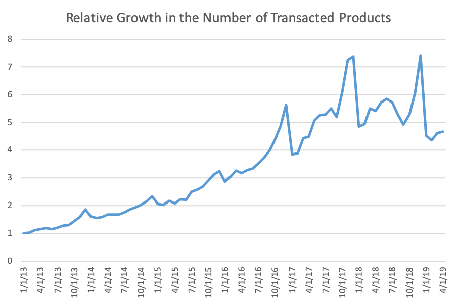
Figure 9. Number of Products in the Current Period over the Base Period.

One key characteristic of our data is the very high turnover of products from month to month, as shown in Figure 8 below. Moreover, Figure 9 shows that there is considerable growth in the selection of products. As discussed in the introduction, these properties motivate the use of the hedonic approach for gauging changes in price levels. The data set we used for this analysis was roughly 20 terabytes because of the number of products and the length of the time period covered. The Spark environment on an EMR cluster was the most appropriate environment to hold and process such large data. The product embeddings and estimation of the hedonic price functions were carried out on a GPU cluster of Amazon Web Services using the Sagemaker notebooks.

Performance for Predicting Prices out-of-Sample

In Table 2 we first examine the predictive performance, recording the R² for predicting prices in the hold-out sample of products. We consider the following methods for estimating the hedonic function:

• linear regression using features generated by a collection of binary encodings of the product catalog;

• linear regression using DL features $W$ and $I$ generated by BERT and ResNet50;

• tree-based (random forest and generalized boosting) regression using DL features $W$ and $I$;

• multi-task neural network regression using DL features $W$ and $I$.

As we can see from Table 2, as we switch from the basic catalog features to using the DL embeddings $W$ and $I$, we obtain the first major improvement, just using linear regression methods. We obtain the second major improvement when we switch from linear regression to a scalable implementation of tree-based methods. Finally, we obtain the final major improvement as we switch from the random forest to the multi-task neural network. Thus, the neural network model easily achieves better predictive performance over other methods.

Figure 4 also presents the month-to-month performance of the various models. The out-of-sample $R^{2}$ for the best multi-task NN model ranges between $80\%$ to $90\%$. Multi-task NN uniformly dominates singe-task NNs, which in turn uniformly dominate boosted tree models and uniformly dominate linear models. The BERT-based multi-task NN nearly uniformly outperforms ELMO-based multi-task NN, although the performance of the two models is generally similar.

The performance of the best models is better at the beginning of the studied period and worsens at the end of the period, perhaps partly due to the increasing variety and number of products being transacted (this is shown in Figure 9). It is worth mentioning that the out-of-sample $R^{2}$ agrees with validation $R^{2}$ we obtained in training (not reported), which is reflective of our training approach that assures that no overfitting happens: we make sure that the training $R^{2}$ and the validation $R^{2}$ are very close.

Method		R2
Linear Model with basic catalogue features	$\approx$	$30-45\%$
Linear Model with DL features $W$ and $I$	$\approx$	$55-65\%$
Random Forest/Boosted Tree Models with DL features $W$ and $I$	$\approx$	$70-80\%$
Single-Task Neural Network with DL features $W$ and $I$	$\approx$	$75-85\%$
Multi-Task Neural Network with DL features $W$ and $I$	$\approx$	$80-90\%$

Table 2. Summary of Out-of-Sample Performance of the Empirical Hedonic Price Function.

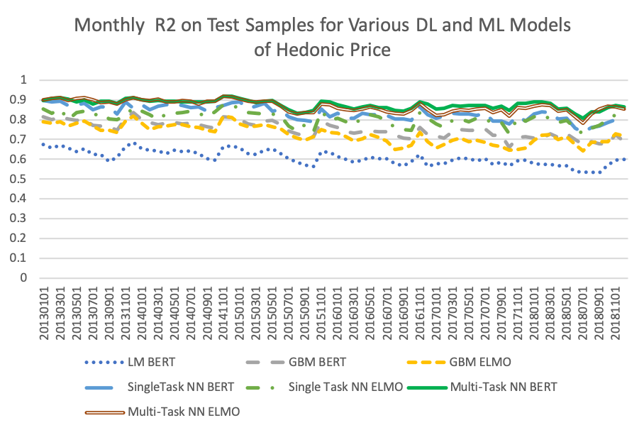
Figure 4. The out-of-sample performance of the empirical hedonic price function obtained using neural network every month since March, 2013. Multi-task neural networks dominate singe-task neural networks, which dominate boosted tree models, which in turn dominate linear models.

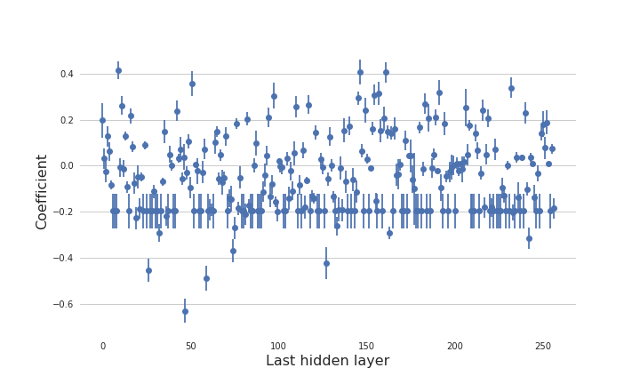
Figure 5. Statistical Significance of Value Embeddings via Linear Regression Model Applied to the Test Sample. The figure shows the point estimates and the pointwise $95\%$ confidence intervals on the coefficients of the value embeddings, as estimated by the linear regression model, applied to the hold-out sample. Note that more than $90\%$ of the coefficients are statistically significant at the $10^{-5}$ level.

Examples of hits and misses

It is instructive to examine the performance of the best NN model through the lenses of particular examples. Here we take one example where the prediction worked well and another where the prediction worked poorly, see Figures 6 and 7. For the first example, a sweater, the NN model predicts the price of this item at about $100$. The time-averaged average price, as shown on camelcamel.com is $97$, with the price ranging from $39$ (corresponding to liquidation events) to $120$. For the second example, a designer dress, the NN predicts the price of this item at about $300$, but the most recent offer prices for this item were around $2400$. While this seems like a major miss, the price history for this item, as seen on camelcamel.com, suggests that there were periods when the price ranged between $206$ and $2800$, with an average sale price of $464$, which is not as far off from our prediction. An important feature that is possibly missed by the NN embeddings is ”cruising around custom rose gold buttons,” although it is hard to verify this feature’s importance objectively.

Figure 6. An example of accurate prediction of (B001GUN1N6): The neural network model predicts the price of this item at about $100$. The average price on camelcamel.com is $97$, with the offer price ranging from $39$ to $120$.

Figure 7. An example of inaccurate prediction: The neural network model predicts the price of this item at about $300$, but the recent offer prices for this product were around $2400$. While this seems a miss, the price history for this item (B06XR39DJ1), that can be seen on camelcamel.com, suggests that there were periods where the offer prices for this item ranged between $206$ and $2800$, with an averaged price of $464$.

Statistical Significance and Inference

Next we examine the hedonic price model’s statistical significance using Section 3.2. We illustrate this approach in Figure 5, which reports the estimated coefficients on value embeddings for the month of November 2018 and reports the component-wise confidence intervals. We also illustrate the construction of the confidence intervals for predicted hedonic price in Table 3, which reports the $90\%$ confidence intervals for estimated hedonic prices for two example products.

Product	Year/Month	$P_{it}$	$\widehat{H}_{it}$	$\mathrm{SE}_{it}$	$[L_{it}(H_{it}),$ $U_{it}(H_{it})]$	$[L_{it}(P_{it}),$ $U_{it}(P_{it})]$
B01DJ34PD2	201812	118.8	114.6	0.05	[114.5, 114.7]	[102, 126]
B01MSBDGTL	201812	119.9	110.25	0.06	[110.1, 110.4]	[98 , 122]

Table 3. Examples of Construction of Confidence Intervals for Predicted Hedonic Price $H_{it}=V_{it}^{\prime}\theta_{t}$ and the Sale Price $P_{it}$. Here $\widehat{H}_{it}=V_{it}^{\prime}\hat{\theta}_{t}$ is the estimated hedonic price. The term $\hat{\sigma}^{2}=V_{it}^{\prime}\widehat{\mathrm{Cov}}(\hat{\theta}_{t})V_{it}$ is the square of the standard error, and $[L_{it},U_{it}]=[\widehat{H}_{it}\pm z_{.95}\hat{\sigma}]$ is the $90\%$ confidence interval for $H_{it}$. The predictive confidence interval for $P_{it}$ is $[L_{it}(P_{it}),U_{it}(P_{it})]=[\widehat{H}_{it}\pm z_{1-\alpha/2}\hat{\nu}]$ with $\hat{\nu}^{2}=\hat{\sigma}^{2}+\widehat{\operatorname{Var}}(P_{it}-H_{it})$ . The term $z_{.95}$ is $.95$-th quantile of the standard normal distribution.

5.2. Hedonic Price Indices for Apparel

Here we will use the definitions of hedonic indices introduced in Section 2. For the computation of the hedonic indices we use the best predictive model – the multitask NN model with $W$ and $I$ features, where $W$ features are obtained as BERT embeddings and $I$ features are obtained as ResNet50 embeddings.

In Table 4, we present our main result – the estimates of an average annual rate of inflation in apparel over 2013-2017, via Fisher HPIs (yearly-chained, monthly chained, geometric average of the two), the Jevons Posted PI, the Adobe DPI, and the CPI for apparel in Urban Areas by BLS:

Apparel Indices	Change in Price Index
Fisher Hedonic, Yearly Chaining (FY)	-0.77%
Fisher Hedonic, Monthly Chaining (FM)	-5.32%
Fisher Hedonic, Geometric Mean ($\sqrt{FY\cdot FM}$)	-3.16%
Fisher Matched, Monthly Chaining (FI)	-3.46%
Jevons Posted Price Index, Daily Chained (JPI)	-2.82%
Adobe Digital Price Index, Monthly Chained (DPI)	-1.30%
U.S. Urban Apparel (BLS)	-0.04%

Table 4. Estimates of Average Annual Rate of Inflation in Apparel over four years, 2014-2017: Fisher Hedonic Index, Fisher Matched Index, Jevons Posted Price Index, Adobe DPI, and the BLS Index for Urban Areas. Adobe DPI is based on 2014-2017.

The main conclusions we draw from these results are the following.

• The main index – the yearly-chained FHPI – suggests an average price decline in 2013-2017 of $.77\%$. In contrast, the BLS CPI for apparel suggests that there was very little decline in the price level.
  

• The yearly chained FHPI declines at a slower rate than the matched Fisher index, Adobe DPI, and the monthly-chained FHPI, highlighting the importance of using hedonic adjustment and long chaining.
  

Indeed, the matched index potentially contains a matching bias created by the high turnover of products illustrated in Figure 8. Moreover, as we emphasized in the introduction, the use of hedonic prices allows us to perform ”long” chaining, thereby mitigating the ”chain drift” problem.

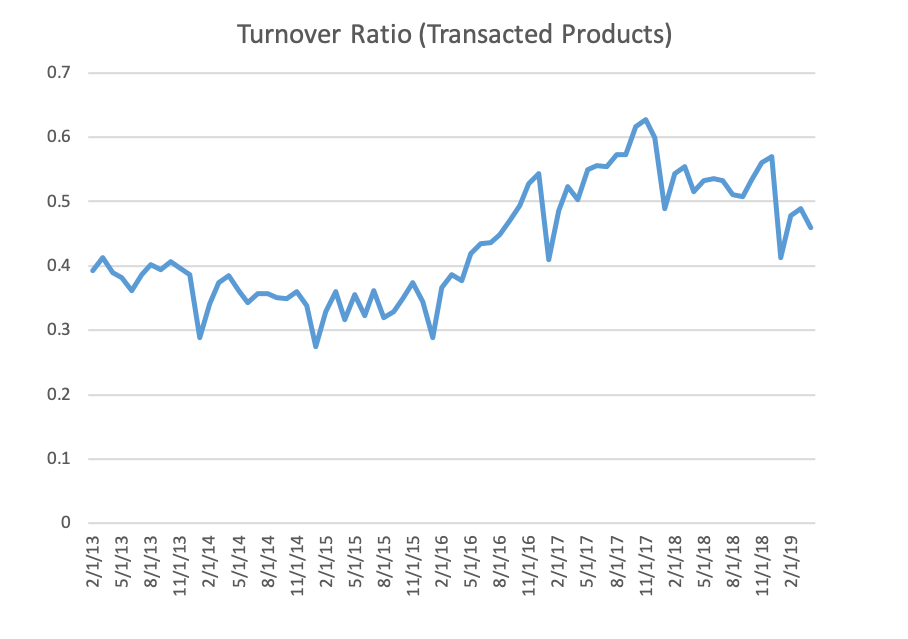
Figure 8. Turnover Rate for Products. The figure shows the ratio of the number of products with transactions in a given month and no transactions in the previous month.

The differences with CPI could be attributed to a number of sources: There are methodological differences: BLS uses a hybrid index where price levels are first measured within narrow subgroups of products, without quantity weighting, and then aggregated by Tornqvist index using expenditure shares for subgroups; moreover, BLS also uses their own hedonic models to perform quality adjustments. Moulton (2018) discusses methodological points and estimates that the upward bias in the overall (non-apparel specific) CPI index may be in the range $[.4\%,1.3\%]$, which could potentially reconcile some of the difference. Other sources of the difference could be the Amazon-specific productivity improvements leading to lower prices (e.g., improvements in supply-chain productivity) and different shares of products in the customers’ baskets.

We also performed similar calculations using a linear model instead of NN (not reported), and conclusions seem qualitatively robust with respect to whether the linear model or nonlinear NN model is used. However, the nonlinear NN models, which do exhibit superior predictive ability, result in a more pronounced quantitative drop in the price index level. For example, the month-over-month chained FHPI index based on the linear model declined 5% less (in absolute terms) over 2013-2017 than the same index based on the NN model. The difference is less drastic than one might expect from having markedly different predictive performance, but the hedonic price index is a ratio of weighted averages of predicted hedonic prices. Since noise gets reduced by averaging, the key determinants of the biases in the index are the weighted averages of biases of the estimated hedonic prices. The NN models are more noisily estimated than the linear models, but they are much less biased giving a better predictive performance as a result. Still, taking weighted averages of prices translates into only “moderate” differences between the indices based on the NN and on the linear models.

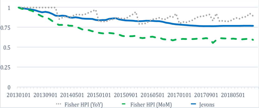
Figure 10. Dynamics of the yearly-chained Fisher Hedonic Price Index (dotted line), the Jevons Price Index (solid lined), and the monthly-chained Fisher Hedonic Price Index (dashed line).

In Figure 10, we demonstrate the dynamics of the year-chained FHPI and compare it with the Jevons index and the monthly chained FHPI.

The Jevons index is a geometric mean of the posted price relatives and does not incorporate quantity weighting. The index underlies the Billion Price Project (Cavallo, 2018b) and also employed by statistical agencies as a complementary index (Office of National Statistics, 2020). The index is convenient and easy to construct because it only relies on publicly posted offer prices and does not use quantity information. The index measures the average “within” price level change calculated on a much larger universe of products (with and without transactions). In contrast, the Fisher index reflects both the “within” price change and the “between” price change since it also reflects the substitutions arising from utility-maximizing behavior by customers with budget constraints. The key empirical observations we draw are as follows.

• The Jevons index exhibits steady declines over the studied period, with a total decline of more than $20\%$; the rate of decline is considerably larger and much more implausible than that of the yearly chained FHPI.

This may suggest that either the chain drift or the substitution effects are sufficiently large to matter. Without the ability to do long chaining and (or) without some proxy for quantity information (such as sales rank data), it is doubtful that Jevons-type indices can accurately approximate inflation. Still, the Jevons index continues to be a very important, simple way to gauge large changes in inflation, as the BPP (based on the Jevons index) has amply demonstrated (Cavallo and Rigobon (2016)).

Finally, when we compare yearly-chained FHPI to monthly-chained FHPI, the key observation is as follows:

• The monthly-chained FHPI exhibits strong, very implausible $40\%$ decline in the price level, in sharp contrast to the yearly-chained FHPI.

This observation highlights the importance of mitigating the “chain drift” problem, which appears to be quite severe for the frequently compounded series such as the monthly chained FHPI. For this reason the monthly chained FHPI and other frequently chained indices (matched Fisher and daily-chained Jevons) are highly unlikely to approximate inflation accurately, especially over longer horizons. Of course, as we stressed before for Jevons, these indices can be useful over short horizons to gauge large changes in the price level.

6. Conclusion

We develop empirical AI-based models of hedonic prices and derive hedonic price indices for measuring changes in consumer welfare. To accomplish this, we generate product attributes or features (from text descriptions and images) by deep learning models from AI and then use them to estimate the hedonic price function, again using deep learning. We convert text information about the product to numeric product features using the BERT large language model, fine-tuned on Amazon’s product descriptions, and convert the product image to numerical product features by a pre-trained ResNet50 neural network model. We use a multi-task neural network to produce estimated hedonic prices over many periods using the aforementioned features. All the ingredients to the method rely on publicly available, open-source software components. We apply the models to Amazon’s proprietary data on first-party sales in apparel to estimate the hedonic prices. The resulting hedonic models have high predictive accuracy for several product categories, with the $R^{2}$ ranging from $80\%$ to $90\%$. Our main hedonic index estimates the rate of inflation in apparel to be moderately negative, somewhat lower than the rate estimated by CPI.

We find the performance of AI-based hedonic models quite remarkable for two reasons. First, the high predictive accuracy of our models suggests that the theoretical hedonic price models from economics provide a good approximation of real-world prices. Second, our methods are AI-powered algorithms that are scalable to many products and avoid the significant manual effort required to construct more traditional hedonic price indices. The good performance of these methods suggests that AI-powered methods, particularly our embeddings, can be used to build real-time hedonic price indices using electronic data and facilitate price research in many settings. These methods can also power economic research in many other areas—for example, labor economics, where embeddings can be used to characterize workers’ job-relevant characteristics, or industrial organization, where embeddings can be used to characterize firms and their products. Since all main ingredients of our approach are open-source, publicly-available technology, future scientific pursuits in this direction can readily use these tools or other similar open-source products.

Based on our experience, we believe there are natural directions for further research. First, we found that while images used alone help predict prices, they add very little to prediction accuracy once the text embeddings are included in the model. Therefore, finding better ways or models to leverage image data is an important unresolved problem. Second, an important further research direction is model explainability. When the price of the product changes, we’d like to explain the price change in terms of changing valuations of key attributes. Similarly, when comparing the prices of two products, we would like to attribute the price difference to the valuations of key attributes. Given the non-linearity of the AI-based hedonic models, explainability is not a simple problem. We hope interested researchers take notice of these open problems.

Appendix A Overview of Text Embedding Models

Here we provide a more technical overview of the text embedding models.

First generation: Word2Vec Embeddings

We first recall some basic ideas underlying the Word2Vec algorithm (Mikolov et al., 2013a). Here we rely on notation in Section 4. The goal is to find the $r\times d$ matrix $\omega=\{u_{j}\}_{j=1}^{d},$ representing $d$ words in $r$ dimensional space. The columns are the embeddings for the words.

We can think of a word appearing in sentence as random variable $T$; and we can let $U$ denote the corresponding embedding. Word2Vect trains the word embeddings by predicting the middle word from the words that surround it in word sentences. Given a subsentence $s$ of $K+1$ words, we have a central word $T_{c,s}$ whose identity we have to predict and we have the words $\{T_{o,s}\}$ that surround it. Collapse the embeddings for context words by a sum,

$$\bar{U}_{o}=\frac{1}{K}\sum_{o}U_{o,s},$$

where $U_{o,s}$ is the element of $\omega$ corresponding to the word $T_{o,s}$. This step imposes a drastically simplifying assumption that the context words are exchangeable.

The probability of middle word $T_{c,s}$ being equal to $t$ is modeled via multinomial logit function:

$$p_{s}(t;\pi,\omega):=P\Big{(}T_{c,s}=t\mid\{T_{o,s}\};\omega\Big{)}=\frac{\exp(\pi_{t}^{\prime}\ \bar{U}_{s}(\omega))}{\sum_{\bar{t}}\exp({\pi_{\bar{t}}^{\prime}\ \bar{U}_{s}(\omega)})},$$

where $\pi=(\pi_{1},...,\pi_{d})$ is $m\times d$ matrix conformable parameter vectors defining the choice probabilities. The model constraints $\pi=\omega,$ and estimates $\omega$ by using the maximum quasi-likelihood method:

$$\max_{\omega=\pi}\sum_{s\in\mathcal{S}}\log p_{s}(T_{i,s};\pi,\omega),$$

where the summation is over many examples $\mathcal{S}$ of subsequences $s$. r

In summary, the Word2Vec algorithm transforms text into a vector of numbers that can be used to compactly represent words. The algorithm trains a neural network in a supervised manner such that the contextual information is used to predict another part of the text. For example, let’s say that the title description of the item is: “Hiigoo Fashion Women’s Multi-pocket Cotton Canvas Handbags Shoulder Bags Totes Purses”. The model will be trained using many $n$-word subsentence examples, such that the center word is predicted from the rest. If we just use $K=3$ subsentence examples, then we train the model using the following examples: (Hiigoo,Women’s) $\rightarrow$ Fashion, (Fashion,Multi-pocket)$\rightarrow$ Women’s, (Women’s,Cotton) $\rightarrow$ Multi-pocket, and so on.

We can examine the quality of word embedding by assessing predictive performance for the price prediction tasks. We can also inspect whether embeddings capture word similarity. If we do this, then we find, for example, the following “necktie” and “bowtie” are most similar to the word “tie”, namely the embeddings for these words are most cosine-similar. The embeddings also seem to induce an interesting vector space on the set of words, which seems to encode analogies well. For example, the embedding for the word “briefcase” is most cosine-similar to the artificial latent word

$$\mathrm{Word2Vec(men^{\prime}s)}+\mathrm{Word2Vec(handbag)}-\mathrm{Word2Vec(women^{\prime}s)}.$$

Examples like this and others reported in Mikolov et al. (2013a) supported the idea of summing the embeddings for words in a sentence to produce embeddings for sentences.

Word2vec embeddings were among the first generation of early successful algorithms. These algorithms have been improved by the next generation of NLP algorithms, such as ELMO and BERT, which are discussed next.

Second Generation: ELMO

The Embeddings from Language Models (ELMO) algorithm (Peters et al, 2018) uses the ideas of the Shannon game, where we guess the next word in the sentence $m$ with $n$ words, i.e.

$$p_{k,m}^{f}(t)=P[T_{k+1,m}=t|T_{1,m},...,T_{k,m};\theta]$$

and also uses reverse guessing as well:

$$p_{k,m}^{b}(t)=P[T_{k-1,m}=t|T_{k,m},...T_{n,m};\theta],$$

where $\theta$ is a parameter vector. Recursive neural networks with single or multiple hidden layers are used to model these probabilities. Parameters are estimated using quasi-maximum log-likelihood methods, where the forward and backward log quasi-likelihoods are added together.

To give a simple example, suppose we wanted to grasp the context better in the previous example, so we could, instead of collapsing embeddings for the context word by a sum, assign individual parameters to each context. This would result in a model closely resembling the previous model, but where the order of context words would play a role. For example, we could model

$$P(T_{k,m}=t\mid\{T_{j,m}\}_{j=1}^{k-1})=\frac{e^{\sum_{j=1}^{k-1}\pi_{t,k}^{\prime}U_{k,m}(\omega)}}{\sum_{\bar{t}}e^{\sum_{j=1}^{k-1}\pi_{\bar{t},k}^{\prime}U_{k,m}(\omega)}},$$

and similarly in reverse order. ELMO uses a more sophisticated (and more parsimonious) non-linear recursive nonlinear regression (recurrent neural network) model to build these probabilities, shown in Figure 11.

The basic structure of ELMO is as follows: Given a sentence $m$ of $n$ words, (1) words are mapped to context-free embeddings in $\mathbb{R}^{d}$. (2) A network is trained to predict each word $T_{k,m}$ of a string given (a) words $(T_{1,m},\ldots,T_{k-1,m})$ or (b) words $(T_{k+1,m},\ldots,T_{n,m})$. The objective is to minimize the average over the sum of the log-loss over the $2n-2$ prediction tasks, where the average is taken over all sentences. (3) The embedding of word $T_{k,m}$ is given by a weighted average of outputs of certain hidden neurons corresponding to this word’s entire context. Importantly, the same final logistic (“softmax”) layer is used for prediction objectives (2a) and (2b). Thus the inputs to this layer, which represent the forward and backward context, are constrained to lie in “the same space.”

Figure 11. ELMO Architecture. This is an ELMO network for a string of $4$ words, with $L=2$ hidden layers. Here, the softmax layer (multinomial logit) is a single function mapping each input in $\mathbb{R}^{d}$ to a probability distribution over the dictionary $\Sigma$.

Training

In Figure 11, the output probability distribution $p^{f}_{k}$ is taken as a prediction of $T_{k+1,m}$; similarly $p^{b}_{k}$ is taken as a prediction of $T_{k-1,m}$. The parameters of the network $\theta$ are obtained by maximizing quasi-loglikelihood:

$$\max_{\theta}\sum_{m\in\mathcal{M}}\left(\sum_{k=1}^{n-1}\log p_{k,m}^{f}(T_{k+1,m};\theta)+\sum_{k=2}^{n}\log p^{b}_{k,m}(T_{k-1,m};\theta)\right),$$

where $\mathcal{M}$ is a collection of sentences (titles and product descriptions) in our data set.

Producing embeddings

To produce embeddings from the trained network, each word $t_{k}$ in a sentence $m=(t_{1},...,t_{k})$ is mapped to a weighted average of the outputs of the hidden neurons indexed by $k$:

$$t_{k}\mapsto w_{k}:=\sum_{i=1}^{L}\gamma_{i}w^{f}_{ki}+\bar{\gamma}_{i}w^{b}_{ki}.$$

The embedding for the sentence (or product description) is produced by summing the embeddings for each individual word. The weights $\gamma$ and $\bar{\gamma}$ can be tuned by the neural network performing the final task. In principle, however, the whole network could in principle be plugged in to the network performing the final task and allowed to update.

Second generation: BERT

Bidirectional Encoder Representations from Transformers (BERT) is another contextualized word embedding learned from deep language model (Devlin et al, 2018). It is a successor of ELMO and achieved state-of-art results on multiple NLP tasks, improving somewhat on ELMO. Instead of using Recurrent Neural Network as in ELMO, BERT uses the Transformer structure with attention mechanism (Vaswani et al., 2017) that pays attention to whole sentence or context.

Unlike the language model in ELMO which predicts the next word from previous words, the BERT model is trained on two self-supervised tasks simultaneously:

• Mask Language Model: randomly mask certain percentage of the words in the sequence and predict the masked words

• Next Sentence Prediction: given a pair of sentences, predict whether one sentence proceeds another.

The structure of BERT model is as follows: (1) Each word in the input sentence is broken to subwords and tokenized using a context-free embedding called WordPiece. A special token $\mathtt{[cls]}$ is added to the beginning of the sequence. And x% of the tokens are replaced by $\mathtt{[mask]}$; (2) For each token, its input representation consists of i) its token embedding from (1), ii) position embedding indicating the position of the token in the sentence, and iii) segment embedding indicating whether it belongs to sentence A or B. (3) The input representation of tokens in the sequence is fed into the main model architecture: L layers of Transformer-Encoder blocks. Each block consists of a multi-head attention layer, followed by a feed forward layer. (4) The output representation of the mask token $\mathtt{[mask]}$ is used to predict the masked word via a softmax layer, and the output representation of the special $\mathtt{[cls]}$ token is used for Next Sentence Prediction. The loss function is a combination of the two losses.

We next focus in detail on the main structure step (3), especially the “multi-head attention” layer.

Computing The Attention

We begin with $n$ word embeddings $(x_{1},x_{2},\ldots,x_{n})$, with each $x_{k}\in\mathbb{R}^{d}$. Let $\mathsf{X}$ denote the matrix whose $k$th row is $x_{k}$. The Multi-Head Attention mapping is applied on $\mathsf{X}$ directly:

$$\mathsf{X}\longmapsto\mathrm{MultiHead}(\mathsf{X},\mathsf{X},\mathsf{X}),$$

where

$$\mathrm{MultiHead}(\mathsf{Q},\mathsf{K},\mathsf{V})=\mathrm{Concatenate}(\mathrm{Head}_{1},\dots,\mathrm{Head}_{h})\omega^{O},$$

$$\mathrm{Head}_{i}=\mathrm{Attention}(\mathsf{Q}\omega_{i}^{Q},\mathsf{K}\omega_{i}^{K},\mathsf{V}\omega_{i}^{V}),$$

$$\mathrm{Attention}(\mathsf{\tilde{Q}},\mathsf{\tilde{K}},\mathsf{\tilde{V}})=\mathrm{softmax}\left(\mathsf{\tilde{Q}}\mathsf{\tilde{K}}^{T}/\sqrt{d_{k}}\right)\mathsf{\tilde{V}},$$

where $\omega^{O}$ and $(\omega_{i}^{Q},\omega_{i}^{K},\omega_{i}^{V})$ are matrix parameters, which are trained to maximize the model performance. In other words, each word embedding is replaced by a weighted average of embeddings for all other words, and the weights are learned from the scaled dot-product of different projections of the word embeddings themself. The projection matrices are parameters learned during training.

Figure 12. BERT Architecture

Generating product embeddings

Depending on specific tasks and resources, Devlin et al. (2018) suggested using the BERT embeddings in various ways: 1) use the last layer, second-to-last layer or concatenate last 4 layers of the encoder outputs from the pre-trained BERT model, 2) fine tune the whole BERT model on the downstream task, or 3) train the BERT language model from scratch on the new data. For this study, we choose the feature-based approach and extract the second-to-last layer as embeddings from the pre-trained BERT model. Each product’s text embedding is the average of the embeddings of each word/token from the input text field.

Comparing ELMO and BERT

While ELMO and BERT are both recent breakthroughs in NLP, the former marked the first contextual word embedding trained from deep language model, and the latter was the first contextual word embedding using Transformer architecture. Note that since the BERT paper was published second and could respond directly to the ELMO paper (but not vice-versa), the comparisons are likely to be biased toward the latter.

There appear to be several differences between the two proposals: (1) They use different initial context-free embeddings. (2) ELMO applies an initial convolutional layer to a character embedding, while BERT augments the WordPiece embedding at sub-word level with positional data. ELMO is based on Recurrent Neural Network while BERT is based on Transformer architecture. (3) The ELMO implementation only allows the averaging weights to be fine-tuned, whereas BERT proposes fine-tuning the whole network. The biggest difference lies in the choice of fundamental architecture. RNNs are known for not being able to capture long-term dependencies. The transformer architecture is more efficient at capturing long-range dependencies in the text. Furthermore, ELMO creates context by using the left-to-right and right-to-left language model representations, while in BERT models the entire context simultaneously.

Appendix B Overview of Image Embeddings via ResNet50

The central idea of the ResNet is to exploit ”partial linearity”: traditional nonlinearly generated neurons are combined (or added together) with the previous layer of neurons. More specifically, a building block is to take a standard feed-forward convolutional neural network and add skip connections that bypass two (or one or several) convolution layers at a time. Each skipping step generates a residual block in which the convolution layers predict a residual. Formally each $k$-th residual block is a neural network mapping

$$v\longmapsto(v,\sigma^{0}_{k}(\omega^{0}_{k}v))\longmapsto(v,\sigma^{1}_{k}\circ\omega^{1}_{k}\sigma^{0}_{k}(\omega_{k}v))\longmapsto v+\sigma^{1}_{k}\circ\omega^{1}_{k}\sigma^{0}_{k}(\omega^{0}_{k}v),$$

where $\omega$’s are matrix-valued parameters or “weights”. This can be seen as a special case of general neural network architecture, designed so that it is easy to learn the identity maps (or sub-maps entering the composition of the entire network). Putting together many blocks like these sequentially, we obtain the overall architecture depicted in Figure 13.

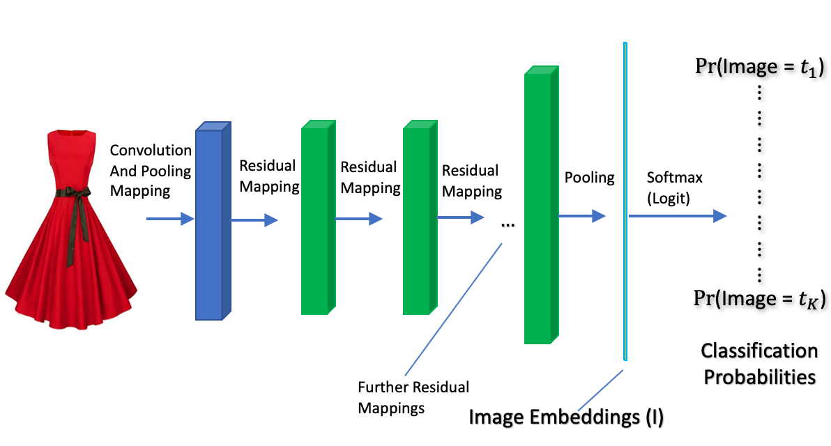
Figure 13. The ResNet50 operates on numerical 3-dimensional arrays representing images. It first does some early processing by applying convolutional and pooling filters, then it applies many residual block mappings, producing arrays shown in green. The penultimate layer produces a high-dimensional vector $I$, the image embedding, which is then used to predict the image type.

The deep feed-forward convolutional networks developed in prior work suffered through major optimization problems – once the depth is high enough, additional layers often resulted in much higher validation and training errors. It was argued that this phenomenon was a result of vanishing gradients, making it difficult to optimize. The residual network architecture addresses this by using the residual block architecture. This possibility allowed high-quality training even for very deep networks.

Just like with text embeddings, we are not interested in the final predictions of these networks but rather in the last hidden layer, which is taken to be the image embedding.

Appendix C Details of Different Architectures for Prediction Using Embeddings

Here we summarize different configurations for neural nets that we’ve tried.

Model 1: ELMO + Single Task Models

The first neural network model we tried is the Single Task model, i.e. predicting product prices one period at a time. For text, we used pre-trained ELMO embedding. For images, we used pre-trained ResNet 50 embedding. The structure is shown in Figure  14. This neural network takes the pre-computed ELMO text embedding (of dimension 256) and the pre-computed ResNet50 image embedding (of dimension 2048) as input, transforms through 1 to 3 fully connected hidden layers with dropout, and a final linear layer maps the last hidden layer of neurons to the one-dimensional output, which is the predicted hedonic price. We trained one model for each time period, so in total there are $T$ neural networks for $T$ time period.

Figure 14. SingleTask + ELMO model. Product text is mapped to $W$ and the image is mapped to $I$ of dimensions $256$ and $2048$. For illustration purposes, we only show two hidden layers with dimensions 7 and 5 respectively. In practice, we use three layers with dimensions 2048, 1024, and 256. The output is price for one time period $t$.

Model 2: BERT + Multitask model

The second neural network model that we tested is the Multitask NN with pre-trained BERT embeddings. The BERT embeddings are precomputed from a multi-lingual BERT model trained by Google. The input is ResNet50 image embeddings (of dimension 2048) and concatenated BERT sentence embeddings for the title, brand, description, and bullet points (of dimension 768 $\cdot$ 4 = 3072). The multitask NN has 1 to 3 dense layers and the output is a $T$ dimensional vector, which represents the hedonic price for each of the $T$ time periods.

Figure 15. MultiTask + BERT. Product text is mapped to $W$ and image is mapped to $I$ of dimensions $3072$ and $2048$ respectively. For illustration purpose, we only show two hidden layers with dimension 7 and 5 respectively, and output is of dimension 3. In practice, we use three layers with dimension 2048, 1024, and 256, and the output is a price vector over $T=72$ time periods.

Fine-Tuned BERT + Multitask model

In the last experiment, we used the end-to-end training framework to fine-tune a BERT model for hedonic price prediction. The model takes raw product text as input, tokenized using the WordPiece tokenizer and truncated / padded to a maximum sequence length $d_{S}$, and run through a BERT base model which consists of 12 transformer blocks. Then the sequence output (of dimension $d_{S}\times d_{T}$) from the transformer blocks is aggregated through a Global Average Pooling layer to product embedding (of dimension $d_{T}$). Then the product embedding is linearly mapped to the output which is $T$-dimensional hedonic price vector for $T$ time periods. In our experiment, we use $d_{S}=512$ and $d_{T}=768$.

The loss function is the same as in Model 2, which combines the weighted squared error term and a regularization term that controls volatility. The weights from all or some layers of the transformer blocks are fine-tuned for the pricing task. Figure 16 is a simple illustration of the end-to-end BERT + Multitask model structure.

We are experimenting with different numbers of fine-tuned layers. Some initial results show that fine-tuning more layers improve model performance by a large margin, but it also takes much longer to train. This part of the work is not included in this paper, and we are continuing to explore this research direction.

Figure 16. MultiTask + Fine-tuned BERT. Product text (sentence) is tokenized and padded to $X$, where components represent the context-free input embedding plus a positional encoding for a token (word). Then the input is fed into a BERT model which consists of 12 layers of transformer blocks and outputs $T$ dimensional price vector. For illustration purposes, we only show 5 tokens and two transformer blocks.

Appendix D The Role of Price Indices in Measuring Productivity

According to the current estimates of statistical agencies, output per hour worked in the US business sector, an in all major advanced countries, has grown at historically slowest rates (at about .5% per year in the US), down by $2\%$ from the preceding decades. Understanding the slow productivity growth is important both for understanding the economy and for policymakers who formulate future policies to improve living standards and evaluate the effects of past policies (e.g., Boskin and Joergenson, 1997). In productivity measurement, a notional level of quantity is obtained by deflating the total output by the total rate of inflation. If inflation is overstated, the productivity increases are understated, and the observed statistical slow-down may in part be an artifact of the legacy of the official statistical methodology. Indeed, the Boskin commission (Boskin et al 1996), Moulton (2017), Golsbee and Klenow (2018), Greenspan (Kessler, 2019) state that the official indices overstate the inflation, thereby understating the real growth productivity. The productivity measurement relies on the Personal Consumption Expenditure index as a the deflator, constructed by the BEA. This index uses a somewhat different methodology than the CPI index, constructed by BLS, but the two generally produce very similar estimates of inflation. The Boskin commission (Boskin et al 1996) was one of the early work-streams that investigating the measurement of inflation by the statistical agencies, concluding at the time that some of the key issues in official indexed have (I) limited ability to capture substitutions among products due to cost-minimizing behavior of consumers, and (II) limited ability to capture the quality change in the products, which is important for controlling for increasing high rate of exit of new products entry and the exit of the old products. These key issues arise in part due to constraints on how the data is collected (for example, quantity information is not collected by BLS, so the substitution biases are harder to eliminate). The commission estimated the resulting upward bias to be at least $1\%$. BLS methodology has been modified to deal with some the methodological problems, but substantial biases still remain, as evaluated by Moulton (2017). These key issues remain continue to persist, with the recent study by Moulton (2017) attributing the bias in the official indices to the same key sources, and estimating that inflation is overstated by .4$\%$-1.3$\%$. That there is upward bias has also been stated by the former Federal Reserve Chairman Alan Greenspan (Kessler, 2019), who suggest the upward bias could be at around $2\%$. Adobe Digital price index (Goolsbee and Klenow, 2019) is able to address substitution biases by working with quantities and suggests that there is $1.3\%$ upward bias in the BLS estimate for 2014-2017. ADPI is a matched Tornquist (which is very close to Fisher index) and does not deal with the product quality change (product entry and exit). However, using Fenstra’s (1996) approach based on CES preferences, they estimate the bias due to product entry to be at further 1.5-2.5% upward bias in ADPI itself. Our proposed approach addresses limitations (I) and (II) by working with real-time quantity and price information and using quality-adjusted prices and indices constructed using modern AI technology. Our estimates of inflation appears to be generally in line with the Goolsbee and Klenow (2019) bias-corrected ADPI.

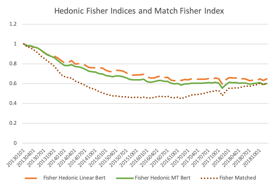
Figure 17. Dynamics of the Monthly Chained Hedonic Fisher Price Index vs Matched Fisher Price index. We show four indices: (1) Fisher HPI constructed using linear model with DL features $W$ and $I$, (2) Fisher HPI constructed using multitask NN model with DL features $W$ and $I$, and (3) Fisher Matched Price Index. All three indices suggest a major decline in price levels, with considerable stabilization in the last four years. Compared to Hedonic Indices the Matched Index experiences a much bigger decline in the middle of the period and the increase at the end period. In contrast, the hedonic index experiences more gradual drops in price levels in early periods and stabilization in the last three years. Given the rather high turnover of products, the hedonic indices are much more credible.

References

- Bajari and Benkard (2005) Patrick Bajari and C Lanier Benkard. Demand estimation with heterogeneous consumers and unobserved product characteristics: A hedonic approach. Journal of political economy, 113(6):1239–1276, 2005. Publisher: The University of Chicago Press.
- Benkard and Bajari (2005) C Lanier Benkard and Patrick Bajari. Hedonic price indexes with unobserved product characteristics, and application to personal computers. Journal of Business & Economic Statistics, 23(1):61–75, 2005. Publisher: Taylor & Francis.
- Berry and Pakes (1999) Steven Berry and Ariel Pakes. Estimating the pure hedonic discrete choice model. Working Paper, Yale University., 1999.
- Berry et al. (1995) Steven Berry, James Levinsohn, and Ariel Pakes. Automobile prices in market equilibrium. Econometrica: Journal of the Econometric Society, pages 841–890, 1995. Publisher: JSTOR.
- Berry et al. (1996) Steven Berry, Samuel Kortum, and Ariel Pakes. Environmental change and hedonic cost functions for automobiles. Proceedings of the National Academy of Sciences, 93(23):12731–12738, 1996. Publisher: National Acad Sciences.
- Berry et al. (2004) Steven Berry, James Levinsohn, and Ariel Pakes. Differentiated products demand systems from a combination of micro and macro data: The new car market. Journal of political Economy, 112(1):68–105, 2004. Publisher: The University of Chicago Press.
- Bils and Klenow (2004) Mark Bils and Peter J Klenow. Some evidence on the importance of sticky prices. Journal of political economy, 112(5):947–985, 2004. Publisher: The University of Chicago Press.
- Boskin and Jorgenson (1997) Michael J Boskin and Dale W Jorgenson. Implications of overstating inflation for indexing government programs and understanding economic progress. The American Economic Review, 87(2):89–93, 1997. Publisher: JSTOR.
- Boskin et al. (1996) Michael J Boskin, Ellen R Dulberger, Zvi Griliches, Robert J Gordon, and Dale Jorgensen. Toward a more accurate measure of the cost of living: final report to the Senate Finance Committee for the advisory commision to study the consumer price index. 1996.
- Boskin et al. (1998) Michael J Boskin, Ellen L Dulberger, Robert J Gordon, Zvi Griliches, and Dale W Jorgenson. Consumer prices, the consumer price index, and the cost of living. Journal of economic perspectives, 12(1):3–26, 1998.
- Breiman (1996) Leo Breiman. Bagging predictors. Machine learning, 24(2):123–140, 1996. Publisher: Springer.
- Breiman (2001) Leo Breiman. Random forests. Machine learning, 45(1):5–32, 2001. Publisher: Springer.
- Cavallo (2017) Alberto Cavallo. Are Online and Offline Prices Similar? Evidence from Large Multi-channel Retailers. American Economic Review, 107(1):283–303, January 2017. ISSN 0002-8282. doi: 10.1257/aer.20160542. URL https://www.aeaweb.org/articles?id=10.1257/aer.20160542.
- Cavallo (2018a) Alberto Cavallo. More Amazon Effects: Online Competition and Pricing Behaviors, October 2018a. URL https://www.nber.org/papers/w25138.
- Cavallo (2018b) Alberto Cavallo. Scraped Data and Sticky Prices. The Review of Economics and Statistics, 100(1):105–119, March 2018b. ISSN 0034-6535. URL https://doi.org/10.1162/REST_a_00652.
- Cavallo and Rigobon (2011) Alberto Cavallo and Roberto Rigobon. The distribution of the size of price changes. Technical report, National Bureau of Economic Research, 2011.
- Cavallo and Rigobon (2016) Alberto Cavallo and Roberto Rigobon. The billion prices project: Using online prices for measurement and research. Journal of Economic Perspectives, 30(2):151–78, 2016.
- Chen and White (1999) Xiaohong Chen and Halbert White. Improved rates and asymptotic normality for nonparametric neural network estimators. IEEE Transactions on Information Theory, 45(2):682–691, 1999. Publisher: IEEE.
- Chernozhukov et al. (2018) Victor Chernozhukov, Mert Demirer, Esther Duflo, and Ivan Fernandez-Val. Generic machine learning inference on heterogeneous treatment effects in randomized experiments, with an application to immunization in india. Technical report, National Bureau of Economic Research, 2018.
- Chernozhukov et al. (2020) Victor Chernozhukov, Alfred Galichon, Marc Henry, and Brendan Pass. Identification of hedonic equilibrium and nonseparable simultaneous equations. Journal of Political Economy, 2020.
- Chessa and Griffioen (2019) Antonio G Chessa and Robert Griffioen. Comparing price indices of clothing and footwear for scanner data and web scraped data. Economie et Statistique, 509(1):49–68, 2019. Publisher: Persée-Portail des revues scientifiques en SHS.
- Chiappori et al. (2010) Pierre-André Chiappori, Robert J McCann, and Lars P Nesheim. Hedonic price equilibria, stable matching, and optimal transport: equivalence, topology, and uniqueness. Economic Theory, 42(2):317–354, 2010. Publisher: Springer.
- Court (1939) AT Court. Hedonic price indexes with automotive examples. In The dynamics of automobile demand, pages 98–119. General Motors Corporation New York, 1939.
- Devlin et al. (2018) Jacob Devlin, Ming-Wei Chang, Kenton Lee, and Kristina Toutanova. Bert: Pre-training of deep bidirectional transformers for language understanding. arXiv preprint arXiv:1810.04805, 2018.
- Diewert (1976) W Erwin Diewert. Exact and superlative index numbers. Journal of econometrics, 4(2):115–145, 1976. Publisher: Elsevier.
- Diewert (1998) W Erwin Diewert. Index number issues in the consumer price index. Journal of Economic Perspectives, 12(1):47–58, 1998.
- Diewert and Fox (2022) W Erwin Diewert and Kevin J Fox. Substitution bias in multilateral methods for cpi construction. Journal of Business & Economic Statistics, 40(1):355–369, 2022.
- Ekeland et al. (2004) Ivar Ekeland, James J Heckman, and Lars Nesheim. Identification and estimation of hedonic models. Journal of political economy, 112(S1):S60–S109, 2004.
- Feenstra (1994) Robert C Feenstra. New product varieties and the measurement of international prices. The American Economic Review, pages 157–177, 1994. Publisher: JSTOR.
- Garcia-Macia et al. (2019) Daniel Garcia-Macia, Chang-Tai Hsieh, and Peter J Klenow. How destructive is innovation? Econometrica : journal of the Econometric Society, 87(5):1507–1541, 2019. Publisher: Wiley Online Library.
- Golosov and Lucas Jr (2007) Mikhail Golosov and Robert E Lucas Jr. Menu costs and Phillips curves. Journal of Political Economy, 115(2):171–199, 2007. Publisher: The University of Chicago Press.
- Goodfellow et al. (2016) Ian Goodfellow, Yoshua Bengio, and Aaron Courville. Deep learning. MIT press, 2016.
- Goodman (1978) Allen C Goodman. Hedonic prices, price indices and housing markets. Journal of urban economics, 5(4):471–484, 1978. Publisher: Elsevier.
- Goodman (1998) Allen C Goodman. Andrew Court and the invention of hedonic price analysis. Journal of urban economics, 44(2):291–298, 1998. Publisher: Elsevier.
- Goolsbee and Klenow (2006) Austan Goolsbee and Peter J Klenow. Valuing consumer products by the time spent using them: An application to the Internet. American Economic Review, 96(2):108–113, 2006.
- Goolsbee and Klenow (2018) Austan D Goolsbee and Peter J Klenow. Internet rising, prices falling: Measuring inflation in a world of e-commerce. In Aea papers and proceedings, volume 108, pages 488–92, 2018.
- Gorodnichenko and Talavera (2017) Yuriy Gorodnichenko and Oleksandr Talavera. Price Setting in Online Markets: Basic Facts, International Comparisons, and Cross-Border Integration. American Economic Review, 107(1):249–282, January 2017. ISSN 0002-8282. doi: 10.1257/aer.20141127. URL https://www.aeaweb.org/articles?id=10.1257/aer.20141127.
- Gorodnichenko et al. (2018) Yuriy Gorodnichenko, Viacheslav Sheremirov, and Oleksandr Talavera. Price Setting in Online Markets: Does IT Click? Journal of the European Economic Association, 16(6):1764–1811, December 2018. ISSN 1542-4766. doi: 10.1093/jeea/jvx050. URL https://doi.org/10.1093/jeea/jvx050.
- Griliches (1961) Z Griliches. Hedonic price indexes for automobiles: an econometric of quality change. Price Statistics Review Committee, 1961.
- Groshen et al. (2017) Erica L Groshen, Brian C Moyer, Ana M Aizcorbe, Ralph Bradley, and David M Friedman. How government statistics adjust for potential biases from quality change and new goods in an age of digital technologies: A view from the trenches. Journal of Economic Perspectives, 31(2):187–210, 2017.
- Han et al. (2021) Sukjin Han, Eric H Schulman, Kristen Grauman, and Santhosh Ramakrishnan. Shapes as product differentiation: Neural network embedding in the analysis of markets for fonts. arXiv preprint arXiv:2107.02739, 2021.
- Handbury et al. (2013) Jessie Handbury, Tsutomu Watanabe, and David E Weinstein. How much do official price indexes tell us about inflation? Technical report, National Bureau of Economic Research, 2013.
- Hausman (2003) Jerry Hausman. Sources of bias and solutions to bias in the consumer price index. Journal of Economic Perspectives, 17(1):23–44, 2003.
- He et al. (2016) Kaiming He, Xiangyu Zhang, Shaoqing Ren, and Jian Sun. Deep residual learning for image recognition. In Proceedings of the IEEE conference on computer vision and pattern recognition, pages 770–778, 2016.
- Heckman et al. (2010) James J Heckman, Rosa L Matzkin, and Lars Nesheim. Nonparametric identification and estimation of nonadditive hedonic models. Econometrica : journal of the Econometric Society, 78(5):1569–1591, 2010. Publisher: Wiley Online Library.
- ILO et al. (2004) ILO, World Bank, et al. Consumer price index manual: Theory and practice. International Labour Organization, 2004.
- Ivancic et al. (2011) Lorraine Ivancic, W Erwin Diewert, and Kevin J Fox. Scanner data, time aggregation and the construction of price indexes. Journal of Econometrics, 161(1):24–35, 2011. Publisher: Elsevier.
- Kaplan and Schulhofer-Wohl (2017) Greg Kaplan and Sam Schulhofer-Wohl. Inflation at the household level. Journal of Monetary Economics, 91:19–38, 2017. Publisher: Elsevier.
- Kidger and Lyons (2020) Patrick Kidger and Terry Lyons. Universal approximation with deep narrow networks. In Conference on learning theory, pages 2306–2327, 2020. tex.organization: PMLR.
- Kingma and Ba (2014) Diederik P Kingma and Jimmy Ba. Adam: A method for stochastic optimization. arXiv preprint arXiv:1412.6980, 2014.
- Klenow and Kryvtsov (2008) Peter J Klenow and Oleksiy Kryvtsov. State-dependent or time-dependent pricing: Does it matter for recent US inflation? The Quarterly Journal of Economics, 123(3):863–904, 2008. Publisher: MIT Press.
- Klenow and Malin (2010) Peter J Klenow and Benjamin A Malin. Microeconomic evidence on price-setting. In Handbook of monetary economics, volume 3, pages 231–284. Elsevier, 2010.
- Lancaster (1966) Kelvin J Lancaster. A new approach to consumer theory. Journal of political economy, 74(2):132–157, 1966.
- LeCun et al. (2015) Yann LeCun, Yoshua Bengio, and Geoffrey Hinton. Deep learning. nature, 521(7553):436–444, 2015. Publisher: Nature Publishing Group.
- McFadden (1974) Daniel McFadden. The measurement of urban travel demand. Journal of public economics, 3(4):303–328, 1974. Publisher: Elsevier.
- Mikolov et al. (2013a) Tomas Mikolov, Kai Chen, Greg Corrado, and Jeffrey Dean. Efficient estimation of word representations in vector space. arXiv preprint arXiv:1301.3781, 2013a.
- Mikolov et al. (2013b) Tomas Mikolov, Ilya Sutskever, Kai Chen, Greg S Corrado, and Jeff Dean. Distributed representations of words and phrases and their compositionality. Advances in neural information processing systems, 26, 2013b.
- Moulton (2018) Brent R Moulton. The measurement of output, prices, and productivity. Report, Productivity Measurement Initiative under The Hutchins Center on Fiscal and Monetary Policy, Brookings Institution, Washington, DC, 2018.
- Nesheim and others (2006) Lars Nesheim and others. Hedonic price functions. CEMMAP, London, 2006.
- Ng (2016) Andrew Ng. Nuts and bolts of building ai applications using deep learning. NIPS Keynote Talk, 2016.
- Office of National Statistics (2020) U.K. Office of National Statistics. Using statistical distributions to estimate weights for web-scraped price quotes in consumer price statistics. Technical report, U.K. Office of National Statistics, September 2020.
- Ohta and Griliches (1976) Makoto Ohta and Zvi Griliches. Automobile prices revisited: Extensions of the hedonic hypothesis. In Household production and consumption, pages 325–398. NBER, 1976.
- Pakes (2003) Ariel Pakes. A reconsideration of hedonic price indexes with an application to PC’s. American Economic Review, 93(5):1578–1596, 2003.
- Peters et al. (2018) Matthew E. Peters, Mark Neumann, Mohit Iyyer, Matt Gardner, Christopher Clark, Kenton Lee, and Luke Zettlemoyer. Deep contextualized word representations, 2018. URL https://arxiv.org/abs/1802.05365. tex.copyright: arXiv.org perpetual, non-exclusive license.
- Stock (1989) James H Stock. Nonparametric policy analysis. Journal of the American Statistical Association, 84(406):567–575, 1989. Publisher: Taylor & Francis.
- Szegedy et al. (2015) Christian Szegedy, Wei Liu, Yangqing Jia, Pierre Sermanet, Scott Reed, Dragomir Anguelov, Dumitru Erhan, Vincent Vanhoucke, and Andrew Rabinovich. Going deeper with convolutions. In Proceedings of the IEEE conference on computer vision and pattern recognition, pages 1–9, 2015.
- Targ et al. (2016) Sasha Targ, Diogo Almeida, and Kevin Lyman. Resnet in resnet: Generalizing residual architectures. arXiv preprint arXiv:1603.08029, 2016.
- Vaswani et al. (2017) Ashish Vaswani, Noam Shazeer, Niki Parmar, Jakob Uszkoreit, Llion Jones, Aidan N Gomez, Łukasz Kaiser, and Illia Polosukhin. Attention is all you need. Advances in neural information processing systems, 30, 2017.
- Wasshausen and Moulton (2006) David Wasshausen and Brent Moulton. The role of hedonic methods in measuring real gdp in the united states. BEA Papers, 67, 2006.
- Yarotsky (2017) Dmitry Yarotsky. Error bounds for approximations with deep ReLU networks. Neural Networks, 94:103–114, 2017. Publisher: Elsevier.
- Zeng (2020) Shipei Zeng. Hedonic imputation with tree-based decision approaches. Working Paper, School of Economics, University of New South Wales, December, 2020.