Bayesian Optimization Meets Self-Distillation

Abstract

Bayesian optimization (BO) has contributed greatly to improving model performance by suggesting promising hyperparameter configurations iteratively based on observations from multiple training trials. However, only partial knowledge (i.e., the measured performances of trained models and their hyperparameter configurations) from previous trials is transferred. On the other hand, Self-Distillation (SD) only transfers partial knowledge learned by the task model itself. To fully leverage the various knowledge gained from all training trials, we propose the BOSS framework, which combines BO and SD. BOSS suggests promising hyperparameter configurations through BO and carefully selects pre-trained models from previous trials for SD, which are otherwise abandoned in the conventional BO process. BOSS achieves significantly better performance than both BO and SD in a wide range of tasks including general image classification, learning with noisy labels, semi-supervised learning, and medical image analysis tasks. Our code is available at https://github.com/sooperset/boss.

1 Introduction

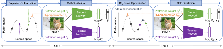
Figure 1: BOSS is a novel framework for training models, which fuses the Bayesian Optimization (BO) and Self-Distillation (SD), combining the concept of hyperparameter exploration and knowledge distillation. By performing these steps simply in an alternating manner (left-to-right), we propagate both the conditional probability learned over hyperparameter configurations (depicted with graphs) and the knowledge learned by each task network, resulting in large performance gains in the final model.

Convolutional Neural Networks (CNNs) have achieved remarkable success in a wide range of computer vision applications [9, 31, 34]. However, their performance is greatly dependent on the choice of hyperparameters [11]. As the optimal hyperparameter configuration is not known a priori, practitioners often explore the hyperparameter space manually to obtain a better configuration. Despite its time-consuming process, it typically results in sub-optimal performance [7]. Recently, Bayesian optimization (BO) has emerged as a successful approach to hyperparameter optimization, automating the manual tuning effort and pushing the boundaries of performance [6, 24, 45]. BO allows for the effective exploration of multi-dimensional search spaces by suggesting promising configurations based on observations. This technique has achieved state-of-the-art performance for training CNNs [8, 15] and has contributed to improving various applications such as AlphaGo [10].

BO is inherently an iterative process in which a probabilistic prior model is fitted using observations of hyperparameter configurations and their corresponding performances [6, 24]. At each iteration, BO suggests the next configuration to evaluate that is most likely to improve performance. After training the network with the suggested configuration, a new observation is retrieved and used to update the probabilistic model. However, only partial knowledge (i.e., the measured performances of trained models and their hyperparameter configurations) from previous trials is transferred, and the knowledge learned by the network is discarded.

Self-distillation (SD) can also be viewed as a knowledge transfer method. A recent line of research in SD has demonstrated that transferring knowledge from a previously trained model with the identical capacity can improve the performance of the model [2, 16, 36]. If a student network is trained to mimic the feature distribution of a teacher network, then the student could beat the teacher. Allen-Zhu and Li [2] have both theoretically and empirically interpreted this as a similar effect to ensembling various models. Inspired by this property of SD and the iterative nature of BO, we ended up asking if the knowledge inside the network from the previous trials could be used for the next trials during the BO process.

In this paper, we propose a new framework, Bayesian Optimization meets Self-diStillation (BOSS), which combines BO and SD to fully leverage the knowledge obtained from previous trials. The overall process of BOSS is illustrated in Figure 1. Following the BO process, BOSS suggests a hyperparameter configuration based on observations that are most likely to improve the performance. After that, it carefully selects pre-trained networks from previous trials for the next round of training with SD, which are otherwise abandoned in the conventional BO process. This process is performed in an iterative manner, allowing the network to persistently improve upon previous trials. To the best of our knowledge, this is the first work that leverages the knowledge of the network learned during the BO process. This is not a simple combination of two orthogonal methods but we provide solutions to the problem of how to transfer past knowledge (i.e., model parameters, hyperparameters, and performances) appropriately. The suggested solution is that (1) not only the teacher but the student should be initialized from the prior knowledge, and (2) they should be initialized from different previous trials to fully exploit the prior knowledge. Our thorough ablation analysis supports this.

We evaluate the effectiveness of BOSS with various computer vision tasks, such as object classification [21], learning with noisy labels [20], and semi-supervised learning [3]. In addition, we also evaluate it with medical image analysis tasks, including medical image classification and segmentation. Our experimental results demonstrate that BOSS significantly improves target model performance, outperforming both BO and SD. Furthermore, we conduct comprehensive analysis and ablation studies to further investigate the behavior of BOSS.

In summary, the main contributions of this paper are:

1. We present BOSS framework that fully harnesses the knowledge from various models by leveraging the benefits of both BO and SD.

2. Exhaustive evaluation experiments demonstrate the efficacy of our framework, as it results in significant performance improvements across diverse scenarios.

3. In-depth analysis and ablation studies provide essential insights into how to transfer prior knowledge effectively for CNNs.

2 Related Work

Bayesian Optimization. Bayesian optimization (BO) is a global optimization method for black-box functions [6]. Given a set of hyperparameters $\lambda$ and an objective function $\Phi$ (e.g. accuracy), BO models the conditional probability $p(\Phi(\lambda)|\lambda)$ with a surrogate model. In each iteration, it fits the surrogate model given observations then uses the acquisition function to determine which configuration to evaluate next. By suggesting probable candidates based on observations, it has shown remarkable performance on various hyperparameter optimization tasks [6, 24, 45]. While other methods [38, 6] models $p(\Phi(\lambda)|\lambda)$, the Tree-structured Parzen Estimator (TPE) [6] models $p(\lambda|\Phi(\lambda))$ by partitioning hyperparameter density function into good and bad groups with respect to their corresponding objective values. It has linear complexity on the number of observations and enables scalable hyperparameter optimization. There have been various approaches to improve BO by incorporating prior knowledge. A line of works aims to transfer knowledge learned from other datasets through meta-learning. Multi-objective TPE [50] extends TPE to transfer knowledge from other tasks considering the similarity between tasks. Surrogate-Based Collaborative Tuning [5] leverages the knowledge from various datasets by integrating the surrogate ranking algorithm into BO. On the other hand, Prior-guided Bayesian Optimization [47] allows domain experts to transfer their knowledge into BO in the form of priors. Our framework is different from these methods in that these utilize prior knowledge from external sources to better estimate the surrogate model, while we utilize the prior knowledge from the given task to enhance the training of the target model. It means that these methods can be applied orthogonally to our framework.

Self-Distillation. Knowledge distillation (KD) is a model compression method that involves transferring the knowledge of a large teacher model to a small student model while maintaining performance. The original work by Hinton et al. [22] proposed distilling knowledge by matching the softmax distribution of the teacher and student models. Since then, various methods have been introduced to improve the knowledge transfer process. Self-Distillation (SD) is a special form of KD where the teacher and student networks have identical architecture. Born-Again Networks (BAN) [16] demonstrated that when training the student to match the output distribution of the teacher with the identical architecture, it could outperform the teacher. Furthermore, they showed that performing multiple rounds of BAN could further improve the performance where the trained student is set to be a new teacher in the following round. The effectiveness of SD has been theoretically explained by the “multi-view” hypothesis introduced by Allen-Zhu and Li, who showed that self-distillation performs an implicit ensemble of various models [2]. Empirical evidence from Pham et al. [36] suggests that SD encourages the student to find flatter minima, leading to better generalization. In this work, we identify that SD can be an effective method for propagating the task knowledge learned in early stages of BO, to late stages of BO. This combination of the SD and BO processes is key to yielding a high-performing model, which we validate experimentally.

3 Method

In this section, we introduce BOSS which combines BO and SD to leverage the knowledge learned in the training trials. We first provide a brief introduction to BO and SD then introduce BOSS in detail.

3.1 Bayesian Optimization

BO is an iterative process that aims to optimize an objective function $\Phi$ with respect to a set of hyperparameters $\lambda$ [24]. At each iteration $t$, BO builds a surrogate model to approximate $\Phi$ based on the observations from the previous iterations, denoted by $\Lambda_{t-1}=\{(\lambda_{0},\Phi(\lambda_{0})),\ldots,(\lambda_{t-1},\Phi(\lambda_{t-1}))\}$. BO then uses an acquisition function $\mu(\lambda|\Lambda_{t-1})$ to select the next hyperparameter configuration $\lambda_{t}$ to evaluate. The acquisition function balances exploration and exploitation, with the most common choice being the Expected Improvement (EI) [25]:

$$\mu(\lambda|\Lambda)=\mathop{\mathbb{E}}(\max\{0,\Phi(\lambda)-\Phi_{\max}\}|\Lambda),$$ (1)

where $\Phi_{\max}$ is the best observed function value. The hyperparameter configuration at iteration $t$ is selected as $\lambda_{t}=\operatorname*{arg\,max}_{\lambda}\mu(\lambda|\Lambda_{t-1})$. After evaluating $\Phi(\lambda_{t})$, the new observation is added to the previous ones, $\Lambda_{t}=\Lambda_{t-1}\cup\{(\lambda_{t},\Phi(\lambda_{t}))\}$, and the surrogate model is updated.

While many surrogate models including the Gaussian process (GP) directly models $p(\Phi(\lambda)|\lambda)$, the Tree-structured Parzen Estimator (TPE) [6] models $p(\lambda|\Phi(\lambda))$ which is defined by two functions:

$$p(\lambda|\Phi(\lambda))\;=\;\left\{\begin{array}[]{rcl}l(\lambda),&{\color[rgb]{0,0,0}\Phi}(\lambda)\;>\;\Phi^{*}\\ g(\lambda),&{\color[rgb]{0,0,0}\Phi}(\lambda)\;\leq\;\Phi^{*}\\ \end{array}\right..$$ (4)

Here, $l(\lambda)$ is the “good” density formed by observations that the performance was higher than a threshold $\Phi^{*}$, $g(\lambda)$ is the “bad” density formed by the remaining observations. Bergstra et al. [6] claims that maximizing EI is proportional to maximizing the ratio of $l(\lambda)/g(\lambda)$. Hence, on iteration $t$, TPE suggests a configuration $\lambda_{t}$ that maximizes this ratio. Despite its simplicity, TPE has outperformed traditional surrogate models such as GP [38].

3.2 Self-Distillation

Furlanello et al. [16] proposed the Self-Distillation (SD) technique for transferring knowledge from a teacher network to a student network with the same architecture. Given a neural network $f$ initialized with random parameters ${\theta}$, SD first obtains the parameters of the teacher model $\theta^{T}$ by minimizing the task loss $\mathcal{L}_{gt}(f(X;\theta),Y)$ with respect to $\theta$. SD then obtains the parameters of the student model $\theta^{S}$ by minimizing a loss with respect to $\theta$ that balances the task loss $\mathcal{L}_{gt}$ and the distillation loss $\mathcal{L}_{dt}$ as follows:

$$\alpha\mathcal{L}_{gt}(f(X;\theta),Y)+(1-\alpha)\mathcal{L}_{dt}(f(X;\theta),f(X;\theta^{T})),$$ (5)

where $\alpha$ is a hyperparameter for balancing the two losses.

In various image classification tasks, the cross-entropy loss is used to define the task loss $\mathcal{L}_{gt}$ as $\mathcal{L}_{gt}(f(X;\theta),Y)=-\sum Y\log\sigma(f(X;\theta))$, where $\sigma$ is the softmax function. For the distillation loss, in conventional self-distillation, $\mathcal{L}_{dt}$ is defined using the Kullback-Leibler (KL) divergence loss. However, recent work [28] has shown that the mean squared error (MSE) between logits from the student and teacher outperforms the KL divergence loss. The MSE distillation loss is defined as $\mathcal{L}_{dt}(f(X;\theta),f(X;\theta^{T}))=||f(X;\theta^{T})-f(X;\theta)||_{2}^{2}$.

Input: Training data $(X,Y)$; number of total trials $N$; number of warm-up trials $W$; number of candidates $K$; neural network $f$; balance parameter $\alpha$.

Initialize: Sets of observations $\Lambda_{0},\Lambda^{\prime}_{W}=\emptyset$; set of parameters $\Theta_{0}=\emptyset$.

Phase 1: Warm-up

for $t=1,2,\ldots,W$ do

       Draw $\theta_{t}$ from the standard normal distribution

       Find $\lambda_{t}$ that maximizes $\mu(\lambda|\Lambda_{t-1})$

       Obtain $\theta_{t}^{*}$ for $\lambda_{t}$ that minimizes $\mathcal{L}_{gt}$ w.r.t $\theta_{t}$:

$$\theta^{*}_{t}=\operatorname*{arg\,min}_{\theta_{t}}\mathcal{L}_{gt}(f(X;\theta_{t}),Y)$$

       Update $\Lambda$: $\Lambda_{t}=\Lambda_{t-1}\cup\{(\lambda_{t},\Phi(\lambda_{t}))\}$

       Update $\Theta$: $\Theta_{t}=\Theta_{t-1}\cup\{\theta_{t}^{*}\}$.

end for

Phase 2: BOSS Training

for $t=W+1,W+2,\ldots,N$ do

       Randomly select $\theta_{t}^{S},\theta_{t}^{T}\in\textsc{top-}K(\Theta_{t-1})$

       Find $\lambda_{t}$ that maximizes $\mu(\lambda|\Lambda^{\prime}_{t-1})$

       Obtain $\theta_{t}^{*}$ for $\lambda_{t}$ that minimizes Eq. 5 w.r.t $\theta_{t}^{S}$:

$$\theta^{*}_{t}=\operatorname*{arg\,min}_{\theta_{t}^{S}} ~{}\alpha\mathcal{L}_{gt}(f(X;\theta_{t}^{S}),Y)$$

$$+(1-\alpha)\mathcal{L}_{dt}(f(X;\theta_{t}^{S}),f(X;\theta_{t}^{T}))$$

       Update $\Lambda^{\prime}$: $\Lambda^{\prime}_{t}=\Lambda^{\prime}_{t-1}\cup\{(\lambda_{t},\Phi(\lambda_{t}))\}$

       Update $\Theta$: $\Theta_{t}=\Theta_{t-1}\cup\{\theta_{t}^{*}\}$.

end for

Output: $\theta_{\text{best}}\in\Theta_{N}$ showing the best performance.

Algorithm 1 Optimization Process for BOSS

3.3 BOSS Framework

BOSS integrates SD into the BO process in order to incorporate the knowledge learned in former trials. While the proposed framework is applicable to various BO and SD methods (see Section 5), we opt for TPE [6] due to its low computational complexity and scalability to diverse search spaces. In addition, we utilize MSE for our distillation loss as it has been shown to yield better performance than KL divergence while requiring fewer hyperparameters [28]. The overall procedure of BOSS is summarized in Algorithm 1.

In order to perform SD, a teacher network is required to train a student network. However, the absence of any network, in the beginning, poses a cold start problem. To address this issue, a warm-up phase is introduced, which is similar to the regular BO process but with the difference that the trained CNNs are recorded for use in subsequent phases. In the warm-up phase, the neural network is initialized with random parameters $\theta$ and a hyperparameter $\lambda$ is suggested using the acquisition function $\lambda={\operatorname*{arg\,max}}_{\lambda}\mu(\lambda|\Lambda)$ in Equation 1. Training images $X$ and their corresponding labels $Y$ are then used to obtain new parameters $\theta^{*}$ for $\lambda$ by minimizing the task loss $\mathcal{L}_{gt}$. Any task-specific loss can be used such as the cross-entropy loss used in image classification tasks. After training, the performance of the neural network $\Phi(\lambda)$ is computed and the observation $(\lambda,\Phi(\lambda))$ is added to a set of observations $\Lambda$. Also, the obtained parameters $\theta^{*}$ are added to a set of parameters $\Theta$.

In the second phase where BOSS training is performed, an empty set is initialized as a new observation set $\Lambda^{\prime}$, because the training scheme differs from the warm-up phase and the optimal configuration is likely to be different. Given the set of parameters $\Theta$ and the pre-defined number of candidates $K$, the top-$K$ candidates are selected according to the performances in $\Theta$. Among them, two are randomly chosen again to define a student and a teacher. We initialize the teacher $\theta^{T}$ and student $\theta^{S}$ with different parameters as we expect some benefit from aggregating different knowledge from different networks. The effect of this scheme is elaborated further in Section 5.2. After the initialization, the hyperparameter $\lambda$ is suggested in the same procedure as in the warm-up phase. Unlike the warm-up phase, $\theta$ is trained to minimize the loss in Equation 5. Once training is complete, the performance and trained parameters are added to $\Lambda^{\prime}$ and $\Theta$, respectively. This procedure is repeated until the budget $N$ is exhausted. Despite potential concerns that the utilization of pre-trained weights could interfere with BO’s modeling, the previous study [27] has demonstrated that BO is sufficiently robust to the variability of initial weights by randomly initializing them at each trial.

As BOSS training proceeds, the top-$K$ models are updated with the models that incorporate the knowledge of previous trials. These models are then utilized to transfer the knowledge in the follow-up iterations. By iteratively updating the candidates with enhanced networks, BOSS consistently improves performance upon previous trials.

4 Experiments

In this section, we present a comprehensive evaluation of BOSS on a wide range of problems and datasets. We compare it with several other methods in our comprehensive evaluation, including Baseline (conventional training with hyperparameters tuned by human experts), SD (Self-Distillation with MSE distillation loss [28]), Random (Random search for hyperparameter optimization [7]), and BO (Bayesian Optimization with TPE [6]). Motivated by the setting in [32], we define our search space to include learning rate $l$, momentum $1-m$, weight decay $w$ and batch size $b$ where $l,m$ are sampled from $\log[10^{-3},1]$, $w$ from $\log[10^{-5},10^{-2}]$, and $b$ from $[64,256]$. We use an implementation of TPE from the Optuna framework [1] and conduct 128 trials with parallel execution of 8 trials. $K$ and $W$ are set to 8 and 32 respectively which will be further explored in Section 5.1.

In order to ensure a fair comparison with BOSS, we conduct multiple rounds of SD until it reaches saturation and report the highest accuracy obtained among all the rounds. Specifically, we continue the SD process until there is no further improvement in performance for three consecutive rounds. We set the hyperparameter $\alpha=0.5$ for SD, which we find to yield the best performance among $\alpha\in\{0.25,0.5,0.75\}$ on CIFAR-100 [29] with the VGG-16 [44] architecture. However, we empirically observe that the final performance does not vary significantly when the SD process is continued until saturation.

4.1 Object Classification

We first evaluate the effectiveness of BOSS in object classification tasks. Publicly available implementations of classification networks and training procedures are utilized to fairly compare it with the human baseline. We use three standard datasets: CIFAR-10 and CIFAR-100 [29], which are comprised of 50,000 training and 10,000 test images of 10 and 100 object classes, respectively, and Tiny ImageNet [42], which includes 100,000 training and 10,000 validation images across 200 object classes. Consistent with previous works [32, 53], we resize the images in the Tiny ImageNet dataset to 32x32 pixels to align with the training procedure of the CIFAR datasets.

In our experiments, the networks are trained using the stochastic gradient descent (SGD) optimizer for 164 epochs on a single GPU. The baseline hyperparameters include a learning rate of 0.1, a weight decay of 5e-4, a momentum of 0.9, and a batch size of 128. We follow the standard practice [21] for training-time data augmentation by zero-padding each image with 4 pixels, randomly cropping it to the original size, and performing evaluations on the original images.

Method	CIFAR-10	CIFAR-100	Tiny-ImgNet
Baseline	93.75±0.18	74.43±0.49	53.33±0.49
SD	94.21±0.24	76.08±0.28	56.46±0.60
Random	94.06±0.39	75.66±1.30	54.72±0.66
BO	94.52±0.20	76.48±0.17	55.39±0.31
BOSS (Ours)	94.98±0.19	77.69±0.15	58.55±0.35

Table 1: Top-1 accuracy (%) on CIFAR10/100 and Tiny-ImageNet with VGG-16. The reported results are the average and the 95% confidence interval over 5 repetitions.

Performance on different datasets. We train the VGG-16 architecture [44] on the aforementioned three datasets. Table 1 compares the top-1 accuracy with the average and the 95% confidence interval over 5 repetitions. It demonstrates that BOSS exhibits considerably higher accuracy than other methods across all tested datasets. While random search succeeds to improve the performance of the baseline, BO further boosts the performance by adaptively suggesting probable configurations. SD also achieves enhanced performance compared to the baseline as expected. However, the effectiveness of SD and BO varies across datasets. On the other hand, BOSS consistently improves the performance by a large margin, leveraging the advantages of both methods.

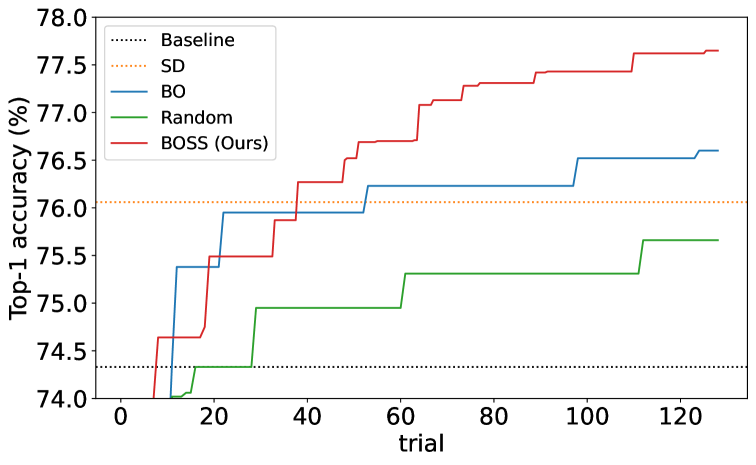
Figure 2: Performance curves of various methods on CIFAR-100 with VGG-16 architecture.

Comparison of diverse methods. We compare the performance of BOSS with other methods in terms of the number of trials. Figure 2 illustrates the performance curves of Random, BO and BOSS along with the Baseline and SD on CIFAR-100 with VGG-16. Throughout the optimization process – except for the initial warm-up phase – BOSS consistently exhibits superior performance over other methods. Initially, all methods display similar performance due to the lack of adequate observations, and BO outperforms random search by exploring promising configurations using previous observations with an increasing number of trials. However, after a certain point, the performance improves at a slow pace. In contrast, BOSS persistently improves upon previous trials by leveraging prior knowledge as a stepping stone to push the performance boundary. This suggests that BOSS’s efficacy is not easily saturated, making it worthwhile for future investigation.

Method	AlexNet	VGG-11	ResNet-20	ResNet-56
Baseline	45.73	71.21	68.92	72.04
SD	46.43	73.27	69.89	75.23
Random	46.07	72.18	68.58	72.19
BO	46.86	73.70	69.84	74.82
BOSS (Ours)	50.61	75.61	72.22	76.26

Table 2: Top-1 accuracy (%) on CIFAR-100 with different network architectures.

Scalability to various architectures. We demonstrate the scalability of BOSS with respect to a variety of CNN architectures including AlexNet [30], VGG-11 [44] and ResNet-20/56 [21] on the CIFAR-100 dataset. As shown in Table 2, BOSS consistently outperforms all other methods across all tested architectures. Notably, even for small networks such as ResNet-20, BOSS achieves superior performance compared to the baseline of larger ResNet-56 with more than three times as many parameters. This finding suggests that BOSS enables efficient network design by achieving better performance with fewer parameters. Moreover, it further brings additional performance improvement to large networks, implying that BOSS is not simply substituting the performance gain by increasing the capacity of the CNN architecture.

Performance with enhanced baseline.

	Baseline	SD	BO	BOSS
CIFAR-10	95.01	95.65	95.79	96.77
CIFAR-100	77.09	78.44	78.07	80.81

Table 3: Top-1 accuracy (%) on CIFAR-10/100 with advanced augmentation methods using VGG-16 architecture.

Pham et al. [36] criticize the existing literature on SD, saying that the performance of reported baselines is not fully saturated. In such cases, the gains achieved through distillation may be invalidated if the baseline is better optimized. Following their suggestion, we incorporate the advanced data augmentations of AutoAugment [12] and Cutout [14]. We train VGG-16 on CIFAR-10/100 using the aforementioned regularizations and report the top-1 validation accuracy in Table 3. As anticipated, the updated data augmentations yield a substantial performance improvement over those in Table 1. Nonetheless, BOSS consistently outperforms other methods by a considerable margin, indicating that the improvements achieved by BOSS are not hindered by better training schemes such as advanced regularization methods.

4.2 Learning with Noisy Labels

Method	Symmetric		Asymmetric
	20%	40%	20%	40%
Baseline	64.79	53.34	63.09	47.44
SD	68.93	59.58	65.73	49.12
BO	65.47	57.52	67.52	56.48
BOSS (Ours)	70.34	65.50	72.82	67.38

Table 4: Comparison with Different Noise Rates on CIFAR-100

We further demonstrate the benefit of BOSS in noisy label settings where incorrect labels exist in training data. In real-world scenarios, the presence of noisy labels often hinder the performance of CNN models [46]. To address this challenge, previous research [2, 26] has demonstrated that employing distillation methods could mitigate the impact of noisy labels by incorporating distinct aspects from multiple teachers to the student. BOSS builds upon this approach by iteratively transferring different knowledge obtained from previous trials.

We conduct experiments to show the robustness of BOSS by training VGG-16 on CIFAR-100 following the training procedure in Section 4.1. Table 4 shows the top-1 accuracy with respect to varying noise ratios and types where symmetric noise refers to the situation where all labels are mixed with the same probability of noise, while asymmetric noise flips labels based on similar class pairs. As expected, the performance of the baseline drops significantly compared to training with the clean dataset in Table 1. While both SD and BO improve the performance of the baseline to some extent, they are sensitive to noise and exhibit performance decreases under large noise conditions. On the other hand, BOSS consistently achieves significant performance improvement regardless of noise levels and types which suggests that the negative influence of label noise can be greatly mitigated by the proposed framework.

4.3 Semi-Supervised Learning

We evaluate BOSS in the context of semi-supervised learning (SSL), where a large amount of unlabeled data is available. Previous works [3, 37, 48, 51] have demonstrated that transferring past knowledge via self-training is an effective approach for utilizing unlabeled data. However, it generally does not exploit the knowledge from various models. We investigate whether BOSS could further enhance the performance by incorporating the knowledge of multiple high-performing models yielded during BO process.

We leverage one of the state-of-the-art SSL method [3] as a baseline and adopt the official implementation. We opt for 13-CNN architecture [4] which is mainly explored in the paper. Table 5 presents the top-1 accuracy of CIFAR-100 dataset with 4,000 and 10,000 labeled data. It is worth noting that the baseline is trained with carefully tuned hyperparameters, advanced regularization techniques, and long training iterations. Nevertheless, BOSS consistently improves the accuracy with a meaningful margin. This result indicates that BOSS could generate a positive synergy with existing SSL algorithm, complementing it by leveraging the knowledge from various models.

	Baseline	SD	BO	BOSS
4,000 labels	63.11	63.80	64.37	65.93
10,000 labels	67.78	69.18	69.31	70.93

Table 5: Top-1 accuracy (%) of semi-supervised learning on CIFAR-100 with varying numbers of labeled data.

4.4 Medical Image Analysis Tasks

The significance of medical image analysis tasks lies in their direct impact on patient outcomes, making their performance a critical concern. One approach to enhance performance in these tasks is to employ multiple models, like model ensembles [23, 19]. However, this can be limited by resource constraints in real-world environments such as hospitals. To tackle this challenge, researchers have turned to HPO techniques such as BO, despite their substantial costs, to improve model performance [39, 17]. Therefore, in this section, we show the efficacy of BOSS on two critical medical image analysis tasks.

The first task we evaluate is breast cancer classification using mammograms, which are x-ray images of the breast used for early cancer detection. Accurate mammographic breast cancer classification is essential, being the primary detection method and the second most common cancer in women. We use two datasets for breast cancer classification with mammograms: the publicly available Chinese Mammography Database [13] (CMMD, 826 exams), and the in-house dataset sourced from the European Union (INH, 6,994 exams). We split each dataset into training sets and validation sets in a 7:3 ratio. We use ResNet-34 to classify mammograms into two categories: cancer or non-cancer. The mammograms are resized to 1920$\times$1280 and applied with various geometric and photometric augmentations, such as translate, rotate, shear, flip, and brightness/contrast adjustment. The model’s performance is evaluated using the Area under the ROC Curve (AUC).

Method	Breast (AUC)		Nuclei (mPQ)
	CMMD	INH	CoNSeP	CPM-17
Baseline	79.22	87.55	51.67	68.03
BO	81.61	87.95	52.88	69.83
BOSS (Ours)	85.81	89.57	53.41	71.66

Table 6: Performance on medical image analysis tasks

Next, we address the task of nuclei instance segmentation, which involves identifying and segmenting individual nuclei in histopathology images. This task is particularly crucial in medical research, as it can assist in the diagnosis and treatment of diseases like cancer. To evaluate the proposed method, we conduct experiments on two datasets: CoNSeP [18] (24,319 instances) and CPM-17 [49] (7,570 instances). To ensure a fair comparison, we train the HoVer-Net [18] architecture, which is a standard architecture in the task, using the official repository and training schemes. The hyperparameter configuration recommended in the original implementation serves as the baseline. We use the multi-class Panoptic Quality (mPQ) [18] metric to evaluate the performance of the model, with higher scores indicating better performance.

Table 6 shows that BOSS outperforms both the baseline and BO methods, achieving enhanced performance on both tasks. This demonstrates that BOSS can efficiently utilize the limited medical image data without any additional overhead at test time via an implicit ensemble of multiple models and superior hyperparameter configuration. It is consistent with the previous findings that have shown model ensembles [52] and hyperparameter optimization [32] to be effective when data is limited. Moreover, the result further shows that the advantage of BOSS is not restricted to classification tasks but could be readily extended to instance segmentation tasks as well. Further extension of BOSS to other tasks such as object detection [34] or generative modeling [40] remains as future work.

5 Ablation Study and Analysis

This section presents ablation studies and analytical experiments to investigate the design choices of BOSS algorithm. We conduct these studies using the same experimental setup as the object classification experiment on VGG-16 with CIFAR-100 presented in Section 4.1.

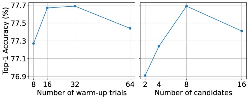
Figure 3: Top-1 accuracy of BOSS on CIFAR-100 with varying the number of (left) warm-up trials and (right) candidates.

BO	PT Student	PT Teacher	Top-1 Accuracy
✓	✗	✗	76.48
✓	✓	✗	76.93
✓	✗	✓	77.18
✓	✓	✓	77.69

Table 7: Comparison of different choices for utilizing pretrained weights on CIFAR-100 with VGG-16. ”PT” stands for ”Pre-trained”.

5.1 Ablation Study

We first examine the impact of the number of warm-up trials $W$ on the performance of BOSS. As BO typically requires a sufficient number of trials to achieve good performance, pretrained models might exhibit low performance when warm up trials are not enough. On the other hand, too many warm-up trials may leave insufficient budget for BOSS training. Figure 3 shows that BOSS performs best with $W=32$, but the performance is not sensitive to $W$. This suggests that the warm-up phase and BOSS phase can complement each other, even with small or large $W$. We further conduct an ablation study on the number of candidates $K$ from which the teacher and student networks are randomly selected. Figure 3 also shows that BOSS achieves the best performance when $K=8$. Choosing a smaller $K$ might limit the performance by not leveraging sufficient knowledge, while selecting a larger $K$ might reduce performance by including weak knowledge from the teacher network.

BOSS leverages pretrained weights for both teacher and student networks to capitalize on past knowledge. In Table 7, we explore different approaches to utilizing pretrained weights during the BO process. When the pretrained weights are loaded only on the student, distillation is not applied. It can be considered as a form of warm restart which has been demonstrated to enhance the performance of DNNs [35]. Employing pretrained weights for either the student or teacher network results in improved performance compared to standard BO. Furthermore, utilizing pretrained weights for both the teacher and student networks leads to even greater performance gains. This indicates that the knowledge of teacher and student could generate a positive synergy.

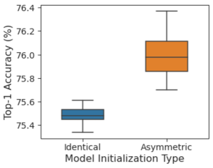
Figure 4: Boxplots of Top-1 accuracy on CIFAR-100 with VGG-16 between identical and asymmetric models. Identical models have the same initialization weights for both teacher and student, while asymmetric models have different initialization weights.

5.2 Effect of Pretrained Weight

In light of our observations that utilizing pretrained weights for both student and teacher networks leads to a improved performance, we note that the Noisy Student [51] reported no improvement in performance when initializing both models simultaneously. They claim that this approach may sometimes lead to getting stuck in a local optima, resulting in inferior performance compared to training the student model from scratch. We hypothesize that this contrasting result could be due to the fact that they used the same pretrained weight for both teacher and student. Since the student model has already inherited all the knowledge that could be learned from the teacher, distilling knowledge with the teacher may not bring additional performance gains.

A recent study by Allen-Zhu and Li [2] revealed that different networks trained with distinct random seeds learn different knowledge. Motivated by this observation, we train VGG-16 on CIFAR-100 with 8 different seeds following the same procedure as the baseline in Section 4.1 and utilize them to initialize teacher and student networks. For all possible combinations of teacher and student networks, we conducted a single-round self-distillation, comparing the top-1 accuracy of the trained models between identical and asymmetric initialization. The identical models refer to initializing both teacher and student with the same pretrained model, while asymmetric models refer to initializing them with different models. The results are presented in Figure 4, which shows boxplots of top-1 accuracy with different initialization types. As expected, utilizing distinct pretrained models for the teacher and student network leads to better performance. Our analysis suggests that it is crucial to initialize the student and teacher network with different models to benefit from warm-starting the student model.

5.3 Different Bayesian Optimization Methods

We verify the effectiveness of BOSS with respect to various BO methods. We perform additional experiments with Gaussian Process (GP) [38] and Sequential Model-based Algorithm Configuration (SMAC) [24]. We utilize publicly available implementations [33] of these methods and adopt their default settings. Table 8 presents the results of our experiments, showing that all BO methods improve the performance of the baseline (i.e. 74.43). BOSS further brings considerable performance improvement in all methods, demonstrating its effectiveness across different BO algorithms.

	TPE	GP	SMAC
BO	76.48	75.69	75.93
BOSS (Ours)	77.69	77.36	77.54

Table 8: Comparison of different Bayesian optimization methods on CIFAR-100 with VGG-16.

5.4 Various Distillation Techniques

	MSE	KL-div.	FitNets	Attention
SD	76.08	75.63	76.19	75.93
BOSS (Ours)	77.69	77.32	77.81	77.35

Table 9: Comparison of different distillation techniques on CIFAR-100 with VGG-16.

We finally evaluate the scalability of BOSS by examining its performance with different distillation techniques. Specifically, we further investigate the efficacy of BOSS with three popular distillation methods: Kullback-Leibler (KL) divergence [22], FitNets [41], and Attention [54]. We follow the suggestion in the original papers for the additional hyperparameters introduced by each distillation loss. Table 9 shows the results of the various distillation methods. We observe that SD successfully enhances the performance of the baseline (i.e. 74.43) across all tested distillation methods, and BOSS further improves the performance significantly. These findings demonstrate that the benefit of BOSS is not limited to specific distillation methods but can be extended to various techniques.

6 Conclusion

In this paper, we present BOSS framework, which combines Bayesian Optimization (BO) and Self-Distillation (SD) to fully leverage the model, hyperparameter configuration, and performance knowledge acquired during the BO process, across all trials. Through extensive experiments in various settings and tasks, we demonstrate that BOSS achieves significant performance improvements, that is consistently better than standard BO or SD on their own. BOSS does not impose any additional overhead at test time and is versatile in that it is applicable to different BO and SD methods. Based on the presented evidence, we believe that the concept of marrying BO and SD is a powerful approach to training models, that should be further explored by the research community.

References

- [1] Takuya Akiba, Shotaro Sano, Toshihiko Yanase, Takeru Ohta, and Masanori Koyama. Optuna: A next-generation hyperparameter optimization framework. In SIGKDD, 2019.
- [2] Zeyuan Allen-Zhu and Yuanzhi Li. Towards understanding ensemble, knowledge distillation and self-distillation in deep learning. arXiv preprint arXiv:2012.09816, 2020.
- [3] Eric Arazo, Diego Ortego, Paul Albert, Noel E O’Connor, and Kevin McGuinness. Pseudo-labeling and confirmation bias in deep semi-supervised learning. In IJCNN, 2020.
- [4] Ben Athiwaratkun, Marc Finzi, Pavel Izmailov, and Andrew Gordon Wilson. There are many consistent explanations of unlabeled data: Why you should average. ICLR, 2019.
- [5] Rémi Bardenet, Mátyás Brendel, Balázs Kégl, and Michele Sebag. Collaborative hyperparameter tuning. PMLR, 2013.
- [6] James Bergstra, Rémi Bardenet, Yoshua Bengio, and Balázs Kégl. Algorithms for hyper-parameter optimization. NeurIPS, 2011.
- [7] James Bergstra and Yoshua Bengio. Random search for hyper-parameter optimization. JMLR, 2012.
- [8] James Bergstra, Daniel Yamins, and David Cox. Making a science of model search: Hyperparameter optimization in hundreds of dimensions for vision architectures. In ICML, 2013.
- [9] Liang-Chieh Chen, George Papandreou, Iasonas Kokkinos, Kevin Murphy, and Alan L Yuille. Deeplab: Semantic image segmentation with deep convolutional nets, atrous convolution, and fully connected crfs. TPAMI, 2017.
- [10] Yutian Chen, Aja Huang, Ziyu Wang, Ioannis Antonoglou, Julian Schrittwieser, David Silver, and Nando de Freitas. Bayesian optimization in alphago. arXiv preprint arXiv:1812.06855, 2018.
- [11] Dami Choi, Christopher J Shallue, Zachary Nado, Jaehoon Lee, Chris J Maddison, and George E Dahl. On empirical comparisons of optimizers for deep learning. arXiv preprint arXiv:1910.05446, 2019.
- [12] Ekin D Cubuk, Barret Zoph, Dandelion Mane, Vijay Vasudevan, and Quoc V Le. Autoaugment: Learning augmentation strategies from data. In CVPR, 2019.
- [13] Chunyan Cui, Li Li, Hongmin Cai, Zhihao Fan, Ling Zhang, Tingting Dan, Jiao Li, and Jinghua Wang. The chinese mammography database (cmmd): An online mammography database with biopsy confirmed types for machine diagnosis of breast. Data Cancer Imaging Arch, 2021.
- [14] Terrance DeVries and Graham W Taylor. Improved regularization of convolutional neural networks with cutout. arXiv preprint arXiv:1708.04552, 2017.
- [15] Stefan Falkner, Aaron Klein, and Frank Hutter. Bohb: Robust and efficient hyperparameter optimization at scale. In ICML, 2018.
- [16] Tommaso Furlanello, Zachary Lipton, Michael Tschannen, Laurent Itti, and Anima Anandkumar. Born again neural networks. ICML, 2018.
- [17] Liyuan Gao and Yongmei Ding. Disease prediction via bayesian hyperparameter optimization and ensemble learning. BMC research notes, 13:1–6, 2020.
- [18] Simon Graham, Quoc Dang Vu, Shan E Ahmed Raza, Ayesha Azam, Yee Wah Tsang, Jin Tae Kwak, and Nasir Rajpoot. Hover-net: Simultaneous segmentation and classification of nuclei in multi-tissue histology images. Medical Image Analysis, 58:101563, 2019.
- [19] Zabit Hameed, Sofia Zahia, Begonya Garcia-Zapirain, Jose Javier Aguirre, and Ana Maria Vanegas. Breast cancer histopathology image classification using an ensemble of deep learning models. Sensors, 20(16):4373, 2020.
- [20] Bo Han, Quanming Yao, Xingrui Yu, Gang Niu, Miao Xu, Weihua Hu, Ivor Tsang, and Masashi Sugiyama. Co-teaching: Robust training of deep neural networks with extremely noisy labels. NeurIPS, 31, 2018.
- [21] Kaiming He, Xiangyu Zhang, Shaoqing Ren, and Jian Sun. Deep residual learning for image recognition. In CVPR, 2016.
- [22] Geoffrey Hinton, Oriol Vinyals, and Jeff Dean. Distilling the knowledge in a neural network. NeurIPS Workshop, 2014.
- [23] Mohamed Hosni, Ibtissam Abnane, Ali Idri, Juan M Carrillo de Gea, and José Luis Fernández Alemán. Reviewing ensemble classification methods in breast cancer. Computer methods and programs in biomedicine, 177:89–112, 2019.
- [24] Frank Hutter, Holger H Hoos, and Kevin Leyton-Brown. Sequential model-based optimization for general algorithm configuration. LION, 2011.
- [25] Donald R Jones, Matthias Schonlau, and William J Welch. Efficient global optimization of expensive black-box functions. Journal of Global optimization, 1998.
- [26] Gal Kaplun, Eran Malach, Preetum Nakkiran, and Shai Shalev-Shwartz. Knowledge distillation: Bad models can be good role models. arXiv preprint arXiv:2203.14649, 2022.
- [27] Jungtaek Kim, Saehoon Kim, and Seungjin Choi. Learning to warm-start bayesian hyperparameter optimization. arXiv preprint arXiv:1710.06219, 2017.
- [28] Taehyeon Kim, Jaehoon Oh, NakYil Kim, Sangwook Cho, and Se-Young Yun. Comparing kullback-leibler divergence and mean squared error loss in knowledge distillation. arXiv preprint arXiv:2105.08919, 2021.
- [29] Alex Krizhevsky, Geoffrey Hinton, et al. Learning multiple layers of features from tiny images. Technical report, 2009.
- [30] Alex Krizhevsky, Ilya Sutskever, and Geoffrey E Hinton. Imagenet classification with deep convolutional neural networks. NeurIPS, 2012.
- [31] HyunJae Lee, Hyo-Eun Kim, and Hyeonseob Nam. Srm: A style-based recalibration module for convolutional neural networks. In ICCV, 2019.
- [32] HyunJae Lee, Gihyeon Lee, Junhwan Kim, Sungjun Cho, Dohyun Kim, and Donggeun Yoo. Improving multi-fidelity optimization with a recurring learning rate for hyperparameter tuning. WACV, 2023.
- [33] Marius Lindauer, Katharina Eggensperger, Matthias Feurer, André Biedenkapp, Difan Deng, Carolin Benjamins, Tim Ruhkopf, René Sass, and Frank Hutter. Smac3: A versatile bayesian optimization package for hyperparameter optimization. JMLR, 2022.
- [34] Wei Liu, Dragomir Anguelov, Dumitru Erhan, Christian Szegedy, Scott Reed, Cheng-Yang Fu, and Alexander C Berg. Ssd: Single shot multibox detector. In ECCV.
- [35] Ilya Loshchilov and Frank Hutter. Sgdr: Stochastic gradient descent with warm restarts. ICLR, 2017.
- [36] Minh Pham, Minsu Cho, Ameya Joshi, and Chinmay Hegde. Revisiting self-distillation. arXiv preprint arXiv:2206.08491, 2022.
- [37] Ilija Radosavovic, Piotr Dollár, Ross Girshick, Georgia Gkioxari, and Kaiming He. Data distillation: Towards omni-supervised learning. In CVPR, pages 4119–4128, 2018.
- [38] Carl Edward Rasmussen, Christopher KI Williams, et al. Gaussian processes for machine learning, volume 1. Springer, 2006.
- [39] Christian Ritter, Thomas Wollmann, Patrick Bernhard, Manuel Gunkel, Delia M Braun, Ji-Young Lee, Jan Meiners, Ronald Simon, Guido Sauter, Holger Erfle, et al. Hyperparameter optimization for image analysis: application to prostate tissue images and live cell data of virus-infected cells. International journal of computer assisted radiology and surgery, 14:1847–1857, 2019.
- [40] Robin Rombach, Andreas Blattmann, Dominik Lorenz, Patrick Esser, and Björn Ommer. High-resolution image synthesis with latent diffusion models. In CVPR, pages 10684–10695, 2022.
- [41] Adriana Romero, Nicolas Ballas, Samira Ebrahimi Kahou, Antoine Chassang, Carlo Gatta, and Yoshua Bengio. Fitnets: Hints for thin deep nets. ICLR, 2015.
- [42] Olga Russakovsky, Jia Deng, Hao Su, Jonathan Krause, Sanjeev Satheesh, Sean Ma, Zhiheng Huang, Andrej Karpathy, Aditya Khosla, Michael Bernstein, et al. Imagenet large scale visual recognition challenge. IJCV, 2015.
- [43] Mattie Salim, Erik Wåhlin, Karin Dembrower, Edward Azavedo, Theodoros Foukakis, Yue Liu, Kevin Smith, Martin Eklund, and Fredrik Strand. External evaluation of 3 commercial artificial intelligence algorithms for independent assessment of screening mammograms. JAMA oncology, 6(10):1581–1588, 2020.
- [44] Karen Simonyan and Andrew Zisserman. Very deep convolutional networks for large-scale image recognition. arXiv preprint arXiv:1409.1556, 2014.
- [45] Jasper Snoek, Hugo Larochelle, and Ryan P Adams. Practical bayesian optimization of machine learning algorithms. NeurIPS, 2012.
- [46] Hwanjun Song, Minseok Kim, Dongmin Park, Yooju Shin, and Jae-Gil Lee. Learning from noisy labels with deep neural networks: A survey. TNNLS, 2022.
- [47] Artur Souza, Luigi Nardi, Leonardo Oliveira, Kunle Olukotun, Marius Lindauer, and Frank Hutter. Prior-guided bayesian optimization. arXiv preprint arXiv:2006.14608, 2020.
- [48] Antti Tarvainen and Harri Valpola. Mean teachers are better role models: Weight-averaged consistency targets improve semi-supervised deep learning results. NeurIPS, 30, 2017.
- [49] Quoc Dang Vu, Simon Graham, Tahsin Kurc, Minh Nguyen Nhat To, Muhammad Shaban, Talha Qaiser, Navid Alemi Koohbanani, Syed Ali Khurram, Jayashree Kalpathy-Cramer, Tianhao Zhao, et al. Methods for segmentation and classification of digital microscopy tissue images. Frontiers in bioengineering and biotechnology, page 53, 2019.
- [50] Shuhei Watanabe, Noow Awad, Masaki Onishi, and Frank Hutter. Multi-objective tree-structured parzen estimator meets meta-learning. arXiv preprint arXiv:2212.06751, 2022.
- [51] Qizhe Xie, Minh-Thang Luong, Eduard Hovy, and Quoc V Le. Self-training with noisy student improves imagenet classification. In CVPR, 2020.
- [52] Pengyi Yang, Yee Hwa Yang, Bing B Zhou, and Albert Y Zomaya. A review of ensemble methods in bioinformatics. Current Bioinformatics, 5(4):296–308, 2010.
- [53] Sukmin Yun, Jongjin Park, Kimin Lee, and Jinwoo Shin. Regularizing class-wise predictions via self-knowledge distillation. In CVPR, 2020.
- [54] Sergey Zagoruyko and Nikos Komodakis. Paying more attention to attention: Improving the performance of convolutional neural networks via attention transfer. ICLR, 2017.