Disagreement amongst counterfactual explanations: How transparency can be deceptive

Abstract

Counterfactual explanations are increasingly used as an Explainable Artificial Intelligence (XAI) technique to provide stakeholders of complex machine learning algorithms with explanations for data-driven decisions. The popularity of counterfactual explanations resulted in a boom in the algorithms generating them. However, not every algorithm creates uniform explanations for the same instance. Even though in some contexts multiple possible explanations are beneficial, there are circumstances where diversity amongst counterfactual explanations results in a potential disagreement problem among stakeholders. Ethical issues arise when for example, malicious agents use this diversity to fairwash an unfair machine learning model by hiding sensitive features. As legislators worldwide tend to start including the right to explanations for data-driven, high-stakes decisions in their policies, these ethical issues should be understood and addressed. Our literature review on the disagreement problem in XAI reveals that this problem has never been empirically assessed for counterfactual explanations. Therefore, in this work, we conduct a large-scale empirical analysis, on 40 datasets, using 12 explanation-generating methods, for two black-box models, yielding over 192.0000 explanations. Our study finds alarmingly high disagreement levels between the methods tested. A malicious user is able to both exclude and include desired features when multiple counterfactual explanations are available. This disagreement seems to be driven mainly by the dataset characteristics and the type of counterfactual algorithm. XAI centers on the transparency of algorithmic decision-making, but our analysis advocates for transparency about this self-proclaimed transparency.

Keywords XAI, Counterfactual Explanations, Machine Learning, Disagreement problem

1 Introduction

Artificial Intelligence (AI) or Machine Learning (ML) is rapidly evolving and disrupting various sectors, such as finance, healthcare, business (e.g., logistics, the labor market), education, and urban development. Besides the many benefits AI can create, multiple negative implications can be identified for each sector [33]. One of the re-occurring challenges concerning AI is the need for transparency: many AI models are opaque and operate on a black-box basis, which makes it difficult - or sometimes impossible - to interpret and explain a decision that has been made. Therefore, Explainable Artificial Intelligence (XAI) has recently emerged as a much-needed research field. Next to an obvious focus on the predictability of AI models, model explainability is necessary for users, developers, and other stakeholders of real-life AI applications. Not only do people generally want to know an explanation for an algorithm-based decision, but also legislation is backing up this need. For example, in 2018 the European Union stated in the new General Data Protection Regulation (GDPR) that subjects of algorithmic decision-making are entitled to explanations. Users can ask for explanations of data-driven decisions that significantly influence their lives [12]. Reaching a certain level of explainability in AI models is possible by either developing models that are inherently better interpretable - but sometimes have less predictive power - or by using post-hoc XAI techniques to generate explanations after predictions have been made with a black-box model.

Even though seemingly good explanations for a model’s decision can be generated by the use of a post-hoc XAI method, and consequently the model and its decisions are qualified as transparent, research on the uniformity of these explanations is rather scarce. Many different post-hoc XAI methods exist and each method can generate different explanations for the same predicted outcome. Ergo, different stakeholders might be more interested in the explanations of one specific XAI method over another one. This raises the question of whether the transparency objective of XAI is achieved. In the literature, this phenomenon has been recently called the disagreement problem [20, 32, 38], on which we will elaborate in Section 2.

[29] takes knowledge from psychology, sociology, and cognitive sciences to identify what are ”good” explanations. They argue that explanations are contrastive, selected, social and that probabilities most likely will not matter. The first means that people generally don’t ask why a certain decision is made. People wonder why a certain decision is made instead of another one. The second points to the fact that even though multiple explanations are possible to justify a decision, people are used to selecting one or two causes as the explanation. The third means an explanation is always dependent on the beliefs of the user and the last refers to the preference of causes over a probability or statistical relationship. These insights stress the usefulness of counterfactual (CF) explanations, a post-hoc example-based XAI method which underlines a set of features that, when changed, alter a decision made by a model [4]. Similarly to other post-hoc XAI techniques, different counterfactual methods might generate different explanations for the same instance and model, which raises ethical questions regarding the use of these techniques.

In this work, we will investigate the extent of the disagreement problem between popular counterfactual explanation methods. In Section 2, we will situate counterfactual explanations in the diverse landscape of post-hoc XAI techniques and express how a lack of consistent evaluation methods for these techniques can lead to ambiguity in their explanations and ethical consequences. Consequently, in Section 3, we will quantify the disagreement amongst ten different counterfactual explanation methods next to Anchor and SHAP. The paper ends with conclusions and future research in Section 4.

2 The diverse landscape of post-hoc explanations

Post-hoc explanation methods are a subcategory of XAI that is concerned with explaining complex black-box models. In contrast to intrinsic explanation methods, they do not try to create interpretable white-box models, but are focused on explaining existing complex models [23]. These methods are particularly interesting because their explanations seem to bypass the accuracy-explainability trade-off [17]. This is a paradox stating that model performance often comes at a cost of model interpretability. However, these post-hoc methods are able to explain complex models and thus theoretically achieve both high performance and explainability at the same time. However, the quality of post-hoc explanation has often been a point of discussion [11, 8].

The difficulty concerning these methods is their evaluation. Because the model is not intrinsically explainable, it is difficult to assess the quality of such explanations. The field of XAI evaluation has come up with different metrics to quantify this quality, however, no consensus has currently been reached. Since we cannot strictly quantify the quality of a post-hoc explanation method, many methods are proposed and used. This has led to ambiguity amongst explanations: explanations for the same instance are different depending on the post-hoc explanation method used (the disagreement problem). The quantified lack of uniformity in explanations has already been investigated for several post-hoc explanation methods [20, 32, 38], however, to the best of our knowledge, this problem has not yet been investigated for counterfactual explanations, which is the main contribution of this work.

We first give an overview and classification of the post-hoc explanation methods used for comparison in this work in Section 2.1. In Section 2.2 we discuss how post-hoc explanation methods are currently evaluated and address some core issues regarding this topic. Lastly, Section 2.3 elaborates on the existing research on the disagreement problem and the need to apply this research to counterfactual explanations.

2.1 Counterfactual explanations and recent post-hoc explanation methods

Post-hoc explanations are techniques to explain AI decisions made after the model has been trained. The most popular methods can be divided into two groups: feature-based techniques (also called attribution methods) and example-based (also called instance-based) techniques [10, 30]. The first group contains methods like local interpretable model-agnostic explanations (LIME), Shapley additive explanations (SHAP), and other feature importance techniques. The second group, example-based post-hoc explanation methods, contains Anchors and counterfactuals. We will briefly explain the methods used in our experiments: SHAP, Anchors, and counterfactual explanations. Figure 1 provides a figurative example of the different XAI methods to explain why a person (the instance) is predicted not to get their loan approved. For a more detailed description and examples, we refer to [30] and the works mentioned below.

(LIME and) SHAP

SHAP [25] and LIME [35] are similar in the sense that the impact of a certain feature is measured related to the predictive outcome. The basic idea of LIME is to sample instances in the neighborhood of the instance that is given to the ML model and then train an interpretable model like linear regression or decision tree to explain this neighborhood. The interpretable model can consequently be used to explain the prediction that is made by the actual, black-box model. For tabular data, which are used in the experiments of this work, the issue is to define the neighborhood of an instance. If LIME would only sample closely around the given instance, chances are high all predictions will be exactly the same and LIME cannot comprehend how predictions change. Therefore, samples are taken broadly, e.g., by using a normal distribution. A major disadvantage of LIME is that the explanations differ depending on the samples used, which makes the explanations unstable and manipulable. Therefore, we do not include LIME in our comparisons.

A better feature-based technique can be found in SHAP, which combines the locality of LIME with the concept of Shapley values from coalitional or cooperative game theory. The contribution of each feature (player) to the prediction that is made by the model (outcome of the game) for a given instance is calculated. Moreover, the contribution of cooperation between players (multiple features) is examined. The average marginal contribution of a feature value across all cooperations is called the shapley value. Because there are $2^{k}$ possible cooperations, for which models need to be trained, calculating all the Shapley values is computationally expensive. Therefore, by using the LIME-inspired sampling, the SHAP algorithm decreases the computation time.

Anchors

Anchors or scoped rules [36] are high-precision easy-to-understand if-then rules. They portray feature conditions together with a predictive outcome. The rules are called Anchors because any changes to other features than the ones mentioned, will not result in another prediction. In contrast to e.g., LIME, Anchors will provide a region of instances to describe the model’s behavior. They are consequently less instance-specific. For example, imagine if a person applies for a loan at a bank. This person is 50 years old, has a monthly income of $2000, his gender is male and he currently has $5000 in debt. A model has predicted that the loan application should be declined. The corresponding Anchor could then be: if the monthly income is lower than $5000 and the age is higher than 35, then predict that the loan application would be accepted.

Counterfactual explanations

Counterfactual explanations describe a combination of feature changes that would alter the predicted class [27]. In other words, they determine what features should change in order to change the prediction and are consequently sometimes called what-if statements. As mentioned in Section 1, this type of explanation is especially human-friendly because they are contrastive and selective [29]. Counterfactual explanations are somewhat the opposite of Anchors. To revisit the same example: the person asking for a loan wants to know why he will not get one. A counterfactual explanation could then be: if your monthly income rises to $5000, you will get a loan. Besides its human-friendly nature, another advantage of the counterfactual method is that it does not need access to the data or the model itself. Only the model’s prediction function is required to generate the explanations. Because of their many benefits, many different counterfactual methods came into existence. [13] and [43] give an overview of counterfactual explanation techniques, however, to date, the state-of-the-art further unfolded with e.g., the introduction of NICE, a counterfactual generation algorithm which simultaneously achieves 100% coverage, model-agnosticism and fast counterfactual generation for different types of classification models.

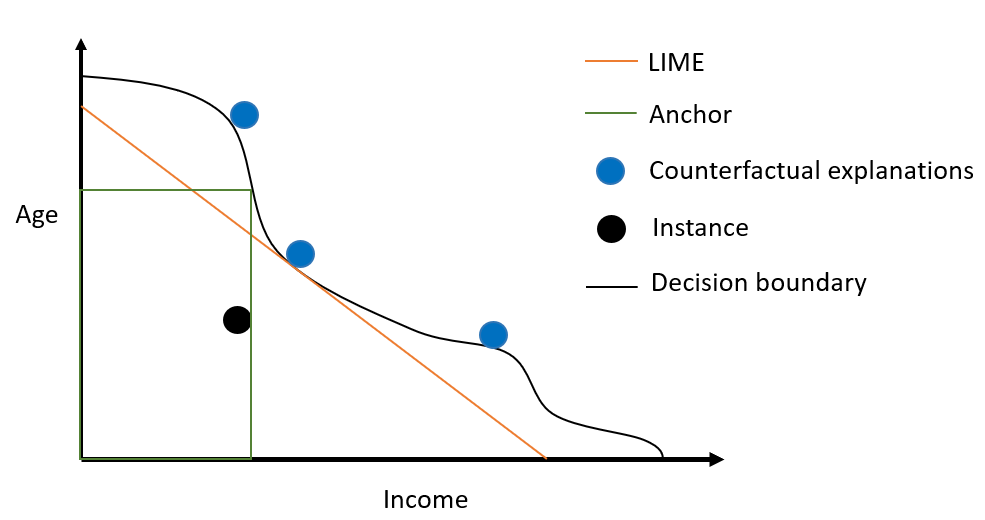
Figure 1: Figurative toy example of LIME, Anchors and counterfactual explanations for a loan approval predictive model, based on [6], [30] and [35]

Feature importance estimates can be biased because it is dependent on the executed sampling [11], while example-based methods like counterfactuals have no additional assumptions or mysteries at the back end of the method. They just tell the user how to change the prediction. On the downside, it is arguable if one instance can fully capture the complexity of a model. Furthermore, the literature recently sees a sprawl of different counterfactual methods, which possibly leads to different respective explanations. The question rises whether these counterfactual methods are still useful for stakeholders and which specific post-hoc explanation method to choose. To answer these questions, the field of XAI evaluation has tried to evaluate the quality of post-hoc explanation methods.

2.2 Ambiguity due to a lack of consistent evaluation metrics for post-hoc explanations

As referred to in Section 1 and Section 2.1, evaluating XAI methods is a research field in its infancy today, even though a strong need for evaluation methods is identified by multiple authors such as [37]. One reason for the limited amount of research done in this field can be the simple fact that evaluating XAI methods is difficult, especially for post-hoc explanation methods. These are designed to explain complex models with a black-box nature. By definition, we don’t know the logic involved in a decision made by such models, thus we cannot compare the output of a post-hoc explanation method to a model’s ground truth. Some have tried generating synthetic datasets for which the ground truth is known [24, 46, 3]. However, this does not completely solve the problem. First of all, the comparison of this ground truth with the explanations is not always straightforward. This results in multiple metrics, for example, [24] look at faithfulness, monotonicity, ROAR, GT-Shapley, and infidelity. Each of these metrics has its own pros and cons. Consequently, the best metric is subjective and application-specific [1]. Secondly, a model might not learn all relationships in the data correctly and show bias. The goal of XAI is to explain the model and not the data. In other words, the model’s ground truth might be different from the data’s ground truth and therefore comparing model explanations with the data’s ground truth can be inaccurate. Lastly, [24] agree with an existing gap between synthetic and real-life datasets. They also cite that using their synthetic datasets and connected ground truths cannot be seen as a replacement for human-centered evaluation of XAI techniques, which is a mostly qualitative way of evaluating explanations.

[44] divide XAI evaluation techniques into two groups: those that involve human-centred evaluations and those that evaluate with objective metrics. The first require human participants to give qualitative or quantitative feedback to XAI explanations, typically through surveys. For the second, to this day, more than 35 metrics have been proposed in the literature to evaluate XAI explanations. Examples of these metrics are, among others, actionability (knowledge is useful to the end-user), efficiency (computational speed of the algorithm), simplification (minimal features), stability (similar instances should provide similar explanations), etc. The authors conclude that the boom in the amount of evaluation metrics calls for a general consensus among researchers on how an explanation should be evaluated.

Note that these objective metrics are sometimes hard to quantify. Qualitative quality properties are therefore often quantified in numbers. For counterfactual explanations, popular properties are proximity, sparsity, and plausibility [43]. Proximity is a property that is somehow used in every counterfactual algorithm. It tries to measure the total change that is suggested by the counterfactual explanations with a distance metric [42, 31, 45]. It is intuitive that less change is better than more change in most situations. Sparsity is a special case of proximity. It refers to the number of features in the explanation [18, 7, 22]. The argument is that shorter explanations are more comprehensible for humans than longer ones [28]. Finally, plausibility is a more conceptual property that refers to the closeness to the data manifold [34]. For example, in a credit scoring context, advising someone to wait 200 years in order to get a loan, is not plausible.

Counterfactual explanations have an additional advantage in comparison to feature importance methods. The latter estimate the influence of each feature on the predicted score. These estimates potentially suffer from bias and features which have almost no influence on the model’s decision might be labeled important [11]. Counterfactual explanations don’t suffer from this bias, applying the suggested changes of a counterfactual explanation will always lead to a change in prediction. Consequently, a counterfactual explanation is always ”correct” in one sense. However, this does not guarantee that these are quality explanations.

The ambiguity of measuring the quality of counterfactual explanations has led to the development of many counterfactual algorithms and possibly as many different explanations [43, 13]. As a result, when a stakeholder now wants to use counterfactual explanations, he is presented with many options. This might be an advantage or can lead to the disagreement problem.

2.3 The disagreement ”problem”

The disagreement problem in explainable AI arises when different interpretability methods, used to explain a given AI model, produce conflicting or contradictory explanations. Because of a lack of broadly used evaluation methods, this is often the case, resulting in explanations that are generally non-consistent and thus ambiguous. [32] raise the question of whether agreement as an evaluation method for XAI methods is suitable. When assuming agreement as an evaluation method, low agreement would mean only a few of the XAI methods are right, while the others are far from ideal. However, low agreement is not necessarily a bad thing.

Ambiguity can actually be valuable or result in possible ethical consequences [26]. It all depends on the context in which XAI methods are used [5]. [31] argues that diversity among counterfactual explanations is beneficial. This for one increases the chance of generating usable explanations. For example, when someone is not allowed to get a loan according to an ML model, and the only counterfactual explanation is to change their sex or lower their level of education, this explanation is not useful. People prefer to get an actionable explanation, such as ’increase your income with $X’. This actionability is not uniform over all decision subjects. Therefore, providing multiple explanations increases the chance that one explanation is useful for this specific user.

[5] examine when ambiguity in explanations is problematic. They differentiate between a cooperative and adversarial context. In a cooperative context, all stakeholders have the same interests. For example, in most medical applications of AI, both doctors and patients have the same goal: to improve or manage the patient’s health. In adversarial contexts, this is not the case. Here, different parties have opposite interests. For example, when a student is denied admission to a prestigious university, the student is interested in challenging this decision. Another example is an autonomous car crashing into a wall to avoid a pedestrian. Insurance companies have other interests than the owner of the car or the developers of the software that steers the car’s driving decisions. Another example is a denied bank loan: the bank and the client have different interests. In these cases, it might not be in the model user’s best interest to look for the most correct or elaborate explanation of a decision that is made. The model user will most likely choose the explanation that fits their best interest, if diverse explanations are available. An adversarial context can lead to all kinds of ethical issues [26]. [2] examine the use of post-hoc explanations to fairwash or rationalize decisions made by an unfair ML model, while [41] and [21] investigate the discriminatory characteristics of explanations. Imagine a model using a prohibited feature such as e.g., gender or race, or a feature that is linked to one of these e.g., zip code, but other more neat explanations are available. The model user could choose to ignore the discriminatory explanations and use another one instead. When considering the ethical consequences of disagreement, consensus amongst explanations might be desired. Therefore, consensus between explanations could be seen as a training objective to increase user trust [40, 16]. Namely, if two explanations are consensual, the ethical consequences of choosing one XAI method over another one are less severe.

2.3.1 Related work

However, these ethical issues can only arise if there actually is ambiguity. The first one to measure the disagreement problem in XAI is [32]. They compare LIME, Integrated Gradients, DeepLIFT, Grad-SHAP, Deep-SHAP, and attention-based explanations with a rank correlation (Kendall’s $\tau$) metric. They conclude there is only low agreement in the explanations of these methods. [20] expand the previous study by comparing LIME, KernelSHAP, Vanilla Gradient, Gradient Input, Integrated Gradients, and SmoothGrad, once again finding disagreement amongst explanation of different methods, especially when the model complexity increases. Instead of only using a rank correlation metric, they use a feature agreement, (signed) rank agreement, sign agreement, and rank correlation. Depending on the type of data (tabular, text or image data), they use different of the above-mentioned evaluation metrics. Next to a quantitative comparison, the authors also perform a qualitative study on how practitioners handle the disagreement problem. 84% of practitioners interviewed by [20] mentioned encountering the disagreement problem on a day-to-day basis. They report there is no principle evaluation method to decide on which explanations to use, therefore, they simply choose to generate explanations with the XAI method they are most familiar with. [14] extend the study of [20] to investigate why the disagreement problem exists for these methods. They conclude that different XAI methods approximate a black-box model over different neighborhoods by applying other loss functions. If two explanations are trained to predict different sets of perturbations, then the explanations are each accurate in their own domain and may disagree. A more focused disagreement problem study can be found in [38] where the explanations of LIME and SHAP are investigated for one single defect prediction model. They calculate the feature, rank, and sign agreement also proposed by [20]. They conclude that LIME and SHAP disagree more on the ranking of important features compared to the sign of their importance.

Authors Nb. of Type of Nb. of Nb. of XAI XAI datasets datasets models methods [32] 5 Text 2 6 LIME, Integrated Gradients, DeepLIFT, Grad-SHAP, Deep-SHAP, and attention-based explanations [20] 4 Tabular, Text and Image 8 6 LIME, Kernel SHAP and Integrated Gradients [38] 4 Tabular 1 2 LIME, SHAP This work 40 Tabular 2 12 SHAP, Counterfactuals and Anchor

Table 1: Literature overview of the quantitative evaluation of the disagreement between post-hoc XAI methods

Table 1 gives an overview of the scarce literature on the quantitative evaluation of disagreement between XAI methods relative to our work. To the best of our knowledge, the disagreement problem has not yet been quantified for counterfactual XAI methods. This is remarkable because recently there has been a boom in the number of such algorithms. [13] identify 60 unique counterfactual algorithms in their recent survey. In this manuscript, we study the disagreement problem between counterfactual explanations for tabular data. We investigate disagreement between 10 selected counterfactual algorithms but also the disagreement with different post-hoc explanation methods such as SHAP [25] and Anchors [36]. Moreover, we extend the size of our study to 40 datasets (instead of 4-5) in order to confidently make more general conclusions.

It should be noted that morally the disagreement problem for counterfactual explanations is similar to the Rashomon effect, introduced by [15]. This effect concerns the diversity in multiple counterfactual explanations generated by the same counterfactual algorithm for the same instance and classifier. One explanation might say to change feature A (e.g., wait 5 years in order to get a loan), while another might say to change feature B while not adapting A (e.g., make sure your income increases with $500 in order to get a loan immediately). This initially seems like a contradiction as well. For example, the DiCE algorithm is focused on generating multiple explanations [31]. In contrast to the Rashomon effect, the disagreement problem investigates diversity amongst different counterfactual explanation algorithms for the same instance and classifier. However, at the heart of the matter, the Rashomon effect and the disagreement problem face the same ethical issues and moral hazards: who chooses which explanation will be used?

3 The quantified disagreement amongst counterfactual explanation methods

In this section, we aim to quantify the disagreement between counterfactual explanation methods. We first illustrate the problem and research questions with an example in Section 3.1. Section 3.2 clarifies the large-scale experimental setup. Section 3.3 answers the research questions by providing metrics to quantify the disagreement amongst counterfactual algorithms and using these metrics in our large-scale experimental setup. Note that measuring the disagreement between counterfactual explanations comes with some new challenges. First of all, counterfactual explanations provide a set of features without ranking them. This makes measures such as (signed) rank agreement useless. Second, counterfactual explanations consist of variable sizes. Some algorithms might suggest six feature changes while others might only suggest two.

3.1 Example

Table 2 illustrates the disagreement problem for an example instance retrieved from the Adult dataset [9]. This dataset can be used to predict if a person would have an annual income higher or lower than $50K. The person depicted in the instances is predicted to have an income lower than $50K. Consequently, ten different counterfactual explanation algorithms generated counterfactual instances in order to tell which features should change in the original instance in order to change the prediction.

Firstly, it should be noted that one of the counterfactual explanation methods, CBR, is not able to find a counterfactual instance for the given original instance, while the others do find one. When having the need to explain a certain instance, it is consequently useful that other explanation methods are able to find explanations and thus, that some disagreement amongst methods is existing. However, in an adversarial context, a malicious counterfactual generating user, wishing to avoid a certain feature e.g., sex or race, is able to do so by simply selecting a counterfactual method that does not include these features, i.e., wants to change these features with respect to the original instance, such as DiCE, NICE(plaus) or NICE(spars). Imagine we are predicting whether or not this person would be qualified to get a loan from a bank. An ML model that uses features like sex or race would then be unethical and discriminatory. The decision maker would be able to hide this fact by secretly choosing a counterfactual method that does not include sex or race in the explanations. This way, the unfair ML model can still be ”rationally” explained. Vice versa, if the malicious user explicitly wants to include a certain feature in an explanation, e.g., hours per week, they can do so with CFproto, NICE(none) or NICE(plaus). And this once again by simply choosing among the diverse explanations, without any need to impose constraints on the counterfactual generating search. This shows the arbitrariness/disagreement of the methods and the power that it brings to the user of counterfactual generating methods. A user can include, as well as avoid, almost any desired feature in the given explanation.

This example clearly illustrates the possible existence of the disagreement problem and the ethical consequences resulting from this existence. In the following sections, we examine how easy it is to abuse the disagreement problem by malicious agents and the driving factors that cause the disagreement problem in the first place.

Workclass Marital Relationship Race Sex Age Fnlwgt Edu. Edu. Occupation Capital Capital Hours Native status num gain loss \week country Instance Local gov. Wid. Other relative Native A/A F 26 195693 1st-4th 9 Craft-repair 0 0 40 France CBR CFproto [gray]0.8Self empl. Wid. [gray]0.8Own-child Native A/A [gray]0.8M [gray]0.844 [gray]0.890688 [gray]0.8Doctorate [gray]0.815 [gray]0.8Other service 0 0 [gray]0.851 [gray]0.8Portugal WIT Local gov. [gray]0.8Never marr. [gray]0.8Unmarried [gray]0.8Black F [gray]0.829 [gray]0.8197932 1st-4th 9 [gray]0.8Handlers-cleaners 0 0 40 [gray]0.8Ecuador GeCo Local gov. [gray]0.8Marr. Other relative [gray]0.8Black F [gray]0.817 [gray]0.8195695 1st-4th 9 Craft-repair 0 0 40 [gray]0.8Hong K. NICE(none) Local gov. Wid. Other relative [gray]0.8Black F [gray]0.843 [gray]0.8112763 1st-4th 9 Craft-repair [gray]0.88614 0 [gray]0.843 [gray]0.8Hong K. NICE(plaus) Local gov. Wid. Other relative [gray]0.8Black F [gray]0.843 [gray]0.8112763 1st-4th 9 Craft-repair [gray]0.88614 0 [gray]0.843 [gray]0.8Hong K. DiCE Local gov. Wid. Other relative Native A/A F [gray]0.850 195693 1st-4th 9 Craft-repair [gray]0.828533 0 40 France NICE(prox) Local gov. Wid. Other relative Native A/A F 26 195693 1st-4th 9 Craft-repair [gray]0.88614 0 40 France NICE(spars) Local gov. Wid. Other relative Native A/A F 26 195693 1st-4th 9 Craft-repair [gray]0.88614 0 40 France SEDC Local gov. [gray]0.8Never marr. [gray]0.8Wife Native A/A [gray]0.8M [gray]0.839 195693 [gray]0.8Masters [gray]0.810 Craft-repair 0 0 40 France
(Edu. = Education, Local gov. = Local government, Wid. = Widowed, Native A/A = Native Alaskan/American, Self empl. = Self employed, Never marr. = Never Married, Marr. = Married, Hong K. = Hong Kong)

Table 2: Example instance (Adult dataset)

3.2 Experimental setup

Table 3 gives an overview of the 40 tabular datasets we use for our study. A test set is created for each dataset by comprising 20% of the data with a minimum of 200 instances. This means that e.g., for the threeOf9 dataset, we do not use 102 instances in the test set, but we use 200. The remaining data is used as the training set for training a Random Forest classifier (RF) and an Artificial Neural Network (ANN). The final two columns of Table 3 display the AUC values obtained for both classifiers. The hyper-parameters of both models are trained using a five-fold cross-validation approach. Subsequently, we generate counterfactual explanations using all algorithms for a random sample of 200 instances from the test set. In total, we generate 200 counterfactual explanations for 10 counterfactual algorithms, Anchors, and SHAP for 2 classifiers on 40 datasets, resulting in a sample size of 192,000 explanations.

Name #Inst. #Feat. #Cat. #Num. Class AUC AUC feat. feat. imbalance (ANN) (RF) adult 48,842 14 5 9 0.761 0.903 0.913 agaricus_lepiota 8154 22 21 1 0.481 1.000 1.000 australian 690 14 7 7 0.445 0.905 0.940 breast_w 699 9 8 1 0.345 0.991 0.997 buggyCrx 690 15 8 7 0.555 0.921 0.949 chess 3196 36 36 0 0.522 1.000 0.999 churn 5000 20 4 16 0.142 0.872 0.919 clean2 6598 168 0 168 0.154 1.000 1.000 coil2000 9822 85 84 1 0.060 0.691 0.745 credit_a 690 15 8 7 0.555 0.902 0.910 credit_g 1000 20 17 3 0.700 0.663 0.731 crx 690 15 8 7 0.445 0.859 0.941 diabetes 768 8 0 8 0.349 0.823 0.851 dis 3772 29 23 6 0.985 0.895 0.989 GAMETES1 1600 20 20 0 0.500 0.636 0.648 GAMETES2 1600 20 20 0 0.500 0.746 0.780 GAMETES3 1600 20 20 0 0.500 0.664 0.722 GAMETES4 1600 20 20 0 0.500 0.690 0.705 german 1000 20 17 3 0.700 0.718 0.758 Hill_Valley 1212 100 0 100 0.505 0.993 0.557 hypothyroid 3163 25 18 7 0.952 0.975 0.988 kr_vs_kp 3196 36 36 0 0.522 1.000 0.999 magic 19,020 10 0 10 0.352 0.922 0.937 mofn_3_7_10 1324 10 10 0 0.779 1.000 1.000 monk1 556 6 6 0 0.500 1.000 1.000 monk2 601 6 6 0 0.342 1.000 0.896 monk3 554 6 6 0 0.520 0.992 0.986 mushroom 8124 22 21 1 0.482 1.000 1.000 parity5+5 1124 10 10 0 0.504 1.000 0.674 phoneme 5404 5 0 5 0.294 0.906 0.970 pima 768 8 0 8 0.349 0.867 0.819 profb 672 9 3 6 0.333 0.633 0.676 ring 7400 20 0 20 0.505 0.990 0.992 spambase 4601 57 0 57 0.394 0.974 0.988 threeOf9 512 9 9 0 0.465 0.972 0.999 tic_tac_toe 958 9 9 0 0.653 0.997 1.000 tokyo1 959 44 2 42 0.639 0.962 0.983 twonorm 7400 20 0 20 0.500 0.996 0.997 wdbc 569 30 0 30 0.371 0.973 0.981 xd6 973 9 9 0 0.331 1.000 1.000

Table 3: Descriptive statistics and performance metrics of all 40 binary datasets.

Name	Author	Spars	Prox	Plaus
CBR	[19]	x		x
CFproto	[42]	x	x	x
WIT	[45]		x	x
GeCo	[39]	x	x	x
NICE (none)	[6]		x	x
NICE (plaus)	[6]	x		x
DiCE	[31]		x
NICE (prox)	[6]		x
NICE (spars)	[6]	x
SEDC	[27]	x

Table 4: Overview of the counterfactual algorithms used for comparison.

We selected a total of 12 post-hoc explanation methods to study the disagreement problem. We focus on ten counterfactual algorithms which are suited for tabular data, are model-agnostic and have their code publicly available. They are depicted in Table 4. The final selection includes the following counterfactual algorithms: DiCe [31], CFproto [42], WIT [45], CBR [19], SEDC [11], GeCo [39] and four types of the NICE algorithm [6] to investigate the uniformity of their explanations. We refer to their respective manuscripts for detailed descriptions of the different counterfactual algorithms. Moreover, we also look at their disagreement with both SHAP and Anchors. As we mentioned in Section 2.2, there is no consensus on what defines the quality of a counterfactual explanation, which resulted in many algorithms optimizing explanations for different evaluation metrics. When we compare algorithms optimized or evaluated for other metrics, some form of disagreement is expected. However, when comparing explanations from algorithms that optimize for the same metric, one might expect less disagreement. We notice two distinct groups in Table 4 (divided by a horizontal line). The first six algorithms optimize for plausibility and the last four do not. The second group is only interested in providing counterfactual instances that are close to the original instance and thus called Prox. The first group is called Plaus.

For the counterfactual explanations, we consider a feature to be present in the explanation if the counterfactual instance indicates to change the feature compared to the original instance. For Anchors we consider a feature present simply when it is mentioned in the Anchor explanation. For SHAP we take into account the seven most important features as features present in an explanation (based on [28]).

3.3 Results

3.3.1 To what extent can counterfactual disagreement be abused by malicious agents?

The main issue with disagreement amongst counterfactual explanations is that malicious users can select certain explanations to rationalize decisions made by unfair or discriminating models. This can be done by either avoiding certain features to convince stakeholders that they are irrelevant or the other way around, by including certain features to insinuate that they are the main driver of the decision-making process.

We first check, how easy it is to exclude a certain feature from a counterfactual explanation. This can be done by looking at the percentage of features that are not present in at least one explanation. Equation 1 formalizes this metric which we call relative feature exclusion. In this metric, the numerator counts the unique features that are not present in the explanations of certain methods $a$ to $n$. This number is divided by the total number of features $F_{D}$ in a dataset $D$. Table 5 and Table 6 show the average relative feature exclusions for different datasets, XAI-methods and classifiers.

$$\textrm{Relative feature exclusion}_{[a,n]}=\frac{|(F_{D}\setminus E_{a})\cup(F_{D}\setminus E_{b})...\cup(F_{D}\setminus E_{n})|}{|F_{D}|}$$ (1)

Next, we investigate the possibility to include a random feature into a counterfactual explanation. For this, we introduce a metric called relative feature span, see Eq. 2. It measures the percentage of all features that is present in at least one explanation. The numerator equals the absolute feature span and measures the size of the union of all explanations of all explanation methods $a$ to $n$ in the comparison. The absolute feature span divided by $F_{D}$ is the relative feature span. A higher feature span most likely results from a higher disagreement amongst methods. Consequently, the user will be able to choose many features as part of the explanation. The maximum relative feature span of 1 is achieved when every single feature is used in at least one explanation. These relative feature spans are shown in Table 7 and Table 8.

$$\textrm{Relative feature span}_{[a,n]}=\frac{|E_{a}\cup E_{b}...\cup E_{n}|}{|F_{D}|}$$ (2)

If we revisit the example of Section 3.1 and assume that the user only has the first two counterfactual explanation algorithms, CFproto and WIT, available. The relative feature exclusion between these two methods amounts $\frac{|(F_{D}\setminus E_{CFproto})\cup(F_{D}\setminus E_{WIT})|}{|F_{Adult}|}$ or 57.1%, meaning that 57.1% of the features can be avoided by the user when using only these two methods. The relative feature span of both methods amounts $\frac{|E_{CFproto}\cup E_{WIT|}}{|E_{Adult}|}$ or 85.7%. This means that 85.7% of the features are present in the explanations of CFproto and WIT, and can consequently be chosen by the user. If all counterfactual explanation methods of Table 2 are available to the user the overall relative feature exclusion equals 100%. This means that any of the features can be chosen to be left out of the explanation if all methods are available to the user. The overall relative feature span equals 92.9%. Only the feature ’capital loss’ is never used in the explanations.

Our results in Table 5 and 6 show that excluding certain features is particularly easy when multiple explanations are available. The average relative feature exclusion is over 99.6% for both classifiers over all counterfactual methods, and 99.8% if we include Anchors and SHAP. For many datasets, the average relative feature exclusion is even 100.0%. Meaning that for every instance that has to be explained, every feature of choice can be excluded from the explanation. These results show that it is fairly easy to avoid sensitive features in order to falsely justify model decisions.

Dataset Prox Plaus All CF All adult 97.8 99.5 100 100 agaricus_lepiota 98.1 100 100 100 australian 99.8 98.9 100 100 breast_w 97.6 97.7 99.6 99.6 buggyCrx 99.2 99.6 100 100 chess 99.7 100 100 100 churn 98 99.1 99.9 100 clean2 99.6 99.3 99.7 99.7 coil2000 99.9 99.9 100 100 credit_a 99.6 97.5 99.9 100 credit_g 99.5 99.8 100 100 crx 99.4 99.4 100 100 diabetes 94.4 92.8 98 98.4 dis 97.6 99.6 99.9 100 GAMETES_1 99.7 100 100 100 GAMETES_2 99.3 99.9 100 100 GAMETES_3 99.7 100 100 100 GAMETES_4 99.6 100 100 100 german 98.8 99.9 100 100 Hill_Valley_without_noise 99.6 99.7 100 100 hypothyroid 98.6 98.9 99.9 100 kr_vs_kp 99.6 100 100 100 magic 93.6 94.6 98.6 99.9 mofn_3_7_10 97.2 99.9 100 100 monk1 97.5 98.3 99.6 99.8 monk2 97.2 98.2 99.8 99.9 monk3 95.1 93.5 96.6 99.1 mushroom 97.8 100 100 100 parity5+5 99.5 99.9 100 100 phoneme 86.8 89.8 97.5 98.9 pima 96.8 90.7 98.3 98.3 profb 98.6 95.5 99.7 100 ring 98.2 99.6 99.9 100 spambase 97.5 99.7 100 100 threeOf9 98.6 98.9 99.8 99.9 tic_tac_toe 99.9 99.2 100 100 tokyo1 99.4 99.5 100 100 twonorm 86.6 99 99.7 99.9 wdbc 98.6 99.3 99.8 100 xd6 98.4 97 99.3 100 Average 97 98.6 99.6 99.9 Standard Deviation 3.4 1.9 0.9 0.2

Table 5: Relative feature exclusion
for the RF classifier

Dataset Prox Plaus All CF All adult 99.4 99.4 100 100 agaricus_lepiota 97.7 97.3 99.8 100 australian 98.4 99.9 100 100 breast_w 99.5 99.6 99.9 100 buggyCrx 98.2 99.9 100 100 chess 99.5 100 100 100 churn 99.4 98.9 99.9 100 clean2 99.9 99.8 100 100 coil2000 99.6 99.7 100 100 credit_a 98.6 99.3 100 100 credit_g 99.2 99.9 100 100 crx 98.2 100 100 100 diabetes 89.8 95.9 97.4 99.9 dis 99.8 100 100 100 GAMETES_1 99.3 100 100 100 GAMETES_2 99.1 99.8 99.9 100 GAMETES_3 99.7 99.9 100 100 GAMETES_4 99.4 100 100 100 german 99 100 100 100 Hill_Valley_without_noise 99.1 100 100 100 hypothyroid 96 99.4 99.8 100 kr_vs_kp 99.4 100 100 100 magic 89.8 96 98.5 100 mofn_3_7_10 98.3 99.9 100 100 monk1 95 98.4 99.4 99.9 monk2 97.4 98.2 99.8 100 monk3 93.3 93.8 95.6 98.8 mushroom 97.4 96.4 99.6 100 parity5+5 99.7 100 100 100 phoneme 92.5 92.9 98.5 99.3 pima 93 98.6 99.4 99.5 profb 95.6 96.4 98.8 100 ring 98.3 98.5 99.9 99.9 spambase 99 100 100 100 threeOf9 98.3 96.7 99.5 99.8 tic_tac_toe 99.1 96.6 99.7 99.9 tokyo1 89.9 100 100 100 twonorm 90.3 99.6 100 100 wdbc 88.2 99.9 100 100 xd6 97.1 94.2 98.1 100 Average 97.8 98.4 99.6 99.8 Standard Deviation 3 2.6 0.8 0.4

Table 6: Relative feature exclusion
for the ANN classifier

Dataset Prox Plaus All CF All adult 40.5 48.4 59.7 74.1 agaricus_lepiota 32.7 53 62.4 65.4 australian 45.3 57.7 63.8 74.1 breast_w 56.8 85.3 87.8 88.9 buggyCrx 29.3 60.8 64.4 75 chess 7.3 17.6 20.3 25.8 churn 47.2 87.9 88.9 93.2 clean2 14.7 92.4 92.8 100 coil2000 17.3 31.3 39.8 41.8 credit_a 41.1 57.6 62.7 75.1 credit_g 27.7 55.3 59.4 65.6 crx 27.1 59.4 64.5 74 diabetes 57.2 89.1 91.8 93.2 dis 17.1 24.4 24.8 49.6 GAMETES_1 17 45 49.8 53 GAMETES_2 15.8 39.4 44.2 67.8 GAMETES_3 16.8 39 43.6 62.3 GAMETES_4 17.4 45.5 50.6 70.6 german 24.4 57.2 60.2 65.7 Hill_Valley_without_noise 17.4 100 100 100 hypothyroid 24.5 27.9 31.6 38.2 kr_vs_kp 7.9 17.6 20.5 26.5 magic 99.9 100 100 100 mofn_3_7_10 31.9 39.9 45.8 57.4 monk1 36.5 42.5 49.5 63.8 monk2 41.1 49.4 59.8 85.8 monk3 24.8 36.9 41.2 60.3 mushroom 30.6 51.8 60.6 64.7 parity5+5 23.8 26.6 38 87.7 phoneme 98.4 100 100 100 pima 64.8 88.2 90.9 99.9 profb 25.2 72.1 73.6 90.1 ring 27.9 100 100 100 spambase 30.3 29.9 35.7 94 threeOf9 25.7 25.4 34.4 56.7 tic_tac_toe 26.2 45.1 52.1 73.5 tokyo1 82.4 81.2 87.9 88 twonorm 100 100 100 100 wdbc 98.4 99.1 100 100 xd6 26.1 21.6 31.1 53.6 Average 37.4 57.5 62.1 73.9 Standard Deviation 25.8 27.1 25.2 21

Table 7: Relative feature span
for the RF classifier

Dataset Prox Plaus All CF All adult 28.2 55.3 61.4 68 agaricus_lepiota 23.6 52.1 57.6 60 australian 36.2 63.8 67 76.5 breast_w 41.4 82.8 87.8 91.2 buggyCrx 24.3 61.6 64.2 65.7 chess 8.6 17.6 21.2 27.8 churn 54.8 88.1 90.9 93.8 clean2 8.4 92.6 93.1 93.1 coil2000 17.6 30 38.3 40.2 credit_a 25 58.5 61.8 73.1 credit_g 20.6 56.9 58.9 65.5 crx 31.3 57.3 63.4 72.1 diabetes 54.8 89.6 92 92.4 dis 17.5 24.8 27.6 29.3 GAMETES_1 17.5 43.8 48.9 71.3 GAMETES_2 15.7 40.2 44.7 66.4 GAMETES_3 16.4 41.6 45.8 65.4 GAMETES_4 16.8 46.1 51 69.5 german 21.6 57.8 61.2 67.4 Hill_Valley_without_noise 21.3 100 100 100 hypothyroid 19.8 28.7 30.9 37.9 kr_vs_kp 9.1 17.5 21.4 28 magic 99.7 100 100 100 mofn_3_7_10 34.2 40.4 46.9 57 monk1 38.7 42.4 52.1 87.5 monk2 44.9 48.8 60 89.3 monk3 32.1 38.5 46.2 61.3 mushroom 26.2 50.3 56.8 62 parity5+5 25.1 33.2 42.4 88.9 phoneme 97.7 99.8 99.9 100 pima 49 90.1 91.4 91.8 profb 35.2 77.1 79.2 92.4 ring 32.7 100 100 100 spambase 29.4 34.9 38.4 40.1 threeOf9 26.1 33.9 42.4 61.9 tic_tac_toe 24.6 58.2 64.8 77.5 tokyo1 73.6 85 85.5 88.4 twonorm 99.9 100 100 100 wdbc 97.8 100 100 100 xd6 26.8 30.2 38.8 58.5 Average 35.6 59.2 63.3 72.8 Standard Deviation 24.8 26 24 21.4

Table 8: Relative feature span
for the ANN classifier

Selecting random features that are desired to be in an explanation seems slightly more difficult. The average relative feature span for all counterfactual methods (depicted in Table 7 and 8) is 62.1% (63.3%) for an RF (ANN) classifier, and 73.9% (72.8%) if we include Anchors and SHAP. However, there are still datasets that have a relative features span of 100.0%. Relative feature spans seem to vary tremendously over different datasets, groups of XAI methods, and classifiers. We refer to Section 3.3.2 for a more detailed examination of the drivers of this counterfactual disagreement.

To conclude, a malicious agent will be easily able to both exclude and include desired features when multiple counterfactual algorithms are available. Especially excluding certain features to hide their influence in the ML model, while still using them to generate predictions, is an almost effortless job.

3.3.2 What are the drivers of counterfactual disagreement?

The disagreement problem makes it easy for malicious agents to exclude or include certain features. While the variation in feature exclusion is minimal, Table 8 and Table 7 showed that feature exclusion does have some variation. In this section, we investigate what are the drivers of this variation. We investigate whether, the dataset, the counterfactual algorithms, or the classifier cause the variation in counterfactual disagreement. This should help to identify when the possibility of feature disagreement is high.

Dataset

Table 8 and Table 7 show that there is a lot of variance over the different datasets. Overall counterfactual explanations, the relative features span varies from around 20 to 100% for both classifiers.

Counterfactual algorithms

As shown in Table 4, the counterfactual algorithms can be divided into two groups plaus and prox. Those that optimize for plausibility, and those that only optimize for plausibility. It might be that the existing disagreement only originates from the disagreement between these groups and not from the disagreement within these groups. To verify this, we also calculated the relative feature span within these groups in Table 8 and 7 and a noticeable difference can be seen. The span within plaus is 20.1 to 23.6% higher compared to the span within the prox group. Figure 2 stresses the difference between the two groups visually by the use of box plots. The center of gravity for the prox group is not only lower but also less broad, compared to the plaus group, meaning that even though the variance stretches over the entire x-axis, the gross of the relative feature spans for this group lies between 22 and 42% (20 and 39%) for the RF (ANN) classifier. In contrast, the relative feature span for the plaus group lies mainly between 39 and 86% (40 and 86%) for the RF (ANN) classifier. This difference can simply be explained by the difference in sparsity between both groups as seen in Table 10. Sparsity refers to the number of features in a counterfactual explanation. Optimizing for proximity (or sparsity directly) has a direct effect on this number of features in the explanations. Therefore, the average sparsity of the prox group is much lower compared to that of the plaus group. Consequently, having fewer features on average in each explanation also results in a lower relative feature span for this group. Furthermore, the plaus group seems to account for most of the feature span of all counterfactual explanations. The difference between the plaus group and the group of all counterfactual explanations is less than 5% for both classifiers.

(a) RF

(b) ANN

Figure 2: Box-plots relative feature span for different algorithm groups for the ANN and RF classifiers

To first have a grasp of how similar the explanations are between different counterfactual algorithms, we examine the pairwise scaled L0 distances between the counterfactual instances of counterfactual methods. This metric counts the number of features that two explanations have in common and divide this number by the total number of features in the dataset.

$$\textrm{L0 distance}_{ab}=\frac{|E_{a}\cap E_{b}|}{F_{D}}$$ (3)

In order to quantify the pairwise disagreement amongst counterfactual explanations, Anchors, and SHAP, we first introduce a new measure called feature disagreement in Eq. 4. This measure is similar to the feature agreement metric introduced by [20] but adapted to the variable explanation sizes of which counterfactuals consist.

$$\textrm{Feature disagreement}_{ab}=\frac{|E_{a}\setminus E_{b}|}{|E_{a}|}$$ (4)

When comparing the explanations $E_{a}$ and $E_{b}$ of two methods $A$ and $B$, the feature disagreement of $A$ with $B$ is equal to the size of the relative complement of $E_{b}$ in $E_{b}$ divided by the size of $E_{a}$. It measures the relative number of features that are in $E_{a}$ but not in $E_{b}$. When the feature disagreement equals 1, none of the features of $E_{a}$ are also in $E_{b}$.

It could be argued that the Jaccard distance can be used to quantify the pairwise disagreement amongst counterfactual methods, this being an existing metric. However, since the feature disagreement metric contains more information regarding the direction of the disagreement, we continue with this metric and refer to Appendix A for the Jaccard distance analysis.

When revisiting the example in Section 3.1, and once again assuming the user only has the first two counterfactual explanation algorithms, CFproto and WIT, available. The pairwise scaled L0 distance between CFproto and WIT equals $\frac{E_{CFproto}\cap E_{WIT}}{F_{Adult}}$ or 35.7%. The feature disagreement between CFproto and WIT equals $\frac{|E_{CFproto}\setminus E_{WIT}|}{|E_{CFproto}|}$ or 50%. CFproto has 50% unique features with respect to WIT. Vice versa, the feature disagreement between WIT and CFproto equals $\frac{|E_{WIT}\setminus E_{CFproto}|}{|E_{WIT}|}$ or 28.6%. WIT has 28.6% unique features with respect to CFproto.

The pairwise scaled L0 distances are shown in Table A1 in Appendix A. We visualized these distances in a 2D-plot by using multidimensional scaling (MDS) in Fig. 3(b) and Fig. 3(a). Note that the numbers on the x- and y-axis of these figures have no translatable meaning, only the relative Euclidean distances between two points are meaningful. The closer two points lie together, the more similar the resulting counterfactual instances of each method are. NICE(prox) and NICE(spars) optimize for very similar metrics with the same optimization method and therefore result in very similar counterfactual instances. The same can be said for NICE(none) and WIT. Both these methods use real instances from the training set in their explanations, and those instances seem to be quite close to each other. Surprisingly, SEDC and CBR are similar as well. GeCo provides counterfactual instances that are the farthest away from all other methods. This might be because GeCo’s explanations contain many features in general. Table 10 shows, that GeCo on average uses around 74% of all features in a single counterfactual explanation.

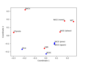
(a) ANN

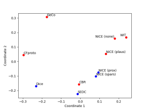
(b) RF

Figure 3: Multidimensional scaling (MDS) for the L0 distance between the counterfactual explanation methods (Blue: Prox, Red: Plaus)

Which algorithms disagree the most with others, while taking into account the number of features present in their explanations, can be identified by looking at the pairwise feature disagreement. Table 9 shows that most post-hoc explanation methods have a high number of features that are not present in CBR, SEDC or SHAP (the darkest columns in Table 9) even though the sparsity of these methods is not necessarily low (see Table 10). Overall GeCo is the counterfactual algorithm that generates the most features that are not available in the explanations of other algorithms. Once again, this can be largely attributed to the fact that GeCo has the highest sparsity, meaning that it has the most features in its generated explanations.

The high feature disagreement of SHAP and Anchors with counterfactual explanations confirms that the disagreement between different post-hoc explanation methods is larger than the disagreement within counterfactual explanations.

Lastly Table 11, presents the average pairwise disagreement between a counterfactual method presented in the first column and the other counterfactual algorithms within the same (intra) and between (inter) group(s). For example, the intra group average for CBR (a member of the plaus group) equals the average of the relative feature disagreements between CBR and the other members of the plaus group: CFproto, WIT, GeCo, NICE(none) and NICE(plaus). On the other hand, the inter group average, amounts the average of the relative feature disagreements between CBR and the members of the prox group: DiCe, NICE(prox), NICE(spars), and SEDC. It is clear that for the plaus group, the intra group averages are significantly lower compared to the inter group averages. In contrast, for the prox group the inter group averages are lower. Since counterfactual algorithms of the prox group generate explanations with less features compared to the other group, chances of disagreement are higher. Vice Versa, it is easier to find agreement when a lot of features are present in the explanantions, which is the case in the plaus group.

RF CBR CFproto WIT GeCo NICE(none) NICE(plaus) DiCE NICE(prox) NICE(spars) SEDC Anchors SHAP Average CBR black!0.00.0 black!37.037.0 black!14.314.3 black!28.928.9 black!15.115.1 black!20.320.3 black!35.435.4 black!25.225.2 black!25.025.0 black!39.139.1 black!12.112.1 black!43.343.3 black!24.624.6 CFproto black!72.072.0 black!0.00.0 black!20.720.7 black!30.330.3 black!20.820.8 black!33.633.6 black!44.544.5 black!45.145.1 black!47.847.8 black!61.561.5 black!34.734.7 black!57.457.4 black!39.039.0 WIT black!81.681.6 black!56.056.0 black!0.00.0 black!40.340.3 black!4.64.6 black!25.825.8 black!64.164.1 black!48.848.8 black!53.553.5 black!78.478.4 black!57.657.6 black!79.779.7 black!49.249.2 GeCo black!87.387.3 black!63.463.4 black!35.735.7 black!0.00.0 black!36.736.7 black!51.051.0 black!70.170.1 black!69.069.0 black!72.772.7 black!82.082.0 black!63.963.9 black!77.977.9 black!59.159.1 NICE(none) black!81.981.9 black!55.755.7 black!4.04.0 black!40.640.6 black!0.00.0 black!22.622.6 black!64.064.0 black!47.247.2 black!52.052.0 black!78.778.7 black!58.058.0 black!80.280.2 black!48.748.7 NICE(plaus) black!78.078.0 black!54.454.4 black!3.53.5 black!41.141.1 black!0.00.0 black!0.00.0 black!60.260.2 black!37.437.4 black!40.240.2 black!70.470.4 black!50.350.3 black!80.280.2 black!43.043.0 DiCE black!80.380.3 black!52.052.0 black!32.532.5 black!43.543.5 black!32.432.4 black!43.443.4 black!0.00.0 black!55.355.3 black!59.459.4 black!71.471.4 black!48.348.3 black!69.769.7 black!49.049.0 NICE(prox) black!75.275.2 black!51.351.3 black!3.03.0 black!42.142.1 black!0.00.0 black!14.314.3 black!54.254.2 black!0.00.0 black!17.217.2 black!66.766.7 black!41.541.5 black!81.981.9 black!37.337.3 NICE(spars) black!72.172.1 black!50.950.9 black!3.33.3 black!43.343.3 black!0.00.0 black!11.811.8 black!53.553.5 black!7.77.7 black!0.00.0 black!63.063.0 black!37.237.2 black!80.980.9 black!35.335.3 SEDC black!63.763.7 black!45.245.2 black!20.220.2 black!35.135.1 black!21.321.3 black!28.128.1 black!40.440.4 black!33.233.2 black!34.334.3 black!0.00.0 black!21.221.2 black!58.258.2 black!33.433.4 Anchors black!80.480.4 black!58.058.0 black!33.933.9 black!50.150.1 black!35.735.7 black!45.345.3 black!55.455.4 black!53.453.4 black!55.955.9 black!67.767.7 black!0.00.0 black!79.079.0 black!51.251.2 SHAP black!89.789.7 black!72.072.0 black!57.757.7 black!59.659.6 black!59.959.9 black!67.767.7 black!73.373.3 black!78.478.4 black!79.179.1 black!82.382.3 black!72.172.1 black!0.00.0 black!66.066.0

ANN CBR CFproto WIT GeCo NICE(none) NICE(plaus) DiCE NICE(prox) NICE(spars) SEDC Anchors SHAP Average CBR black!00 black!39.739.7 black!17.117.1 black!30.930.9 black!17.917.9 black!25.725.7 black!4343 black!32.732.7 black!32.732.7 black!47.547.5 black!21.921.9 black!59.259.2 black!30.730.7 CFproto black!74.374.3 black!00 black!24.824.8 black!36.936.9 black!24.724.7 black!39.639.6 black!51.651.6 black!54.654.6 black!56.756.7 black!66.666.6 black!42.842.8 black!75.375.3 black!45.745.7 WIT black!80.880.8 black!53.553.5 black!00 black!38.938.9 black!4.34.3 black!29.929.9 black!67.367.3 black!55.755.7 black!57.457.4 black!80.280.2 black!59.859.8 black!87.387.3 black!51.351.3 GeCo black!85.785.7 black!56.456.4 black!33.933.9 black!00 black!34.634.6 black!53.153.1 black!65.865.8 black!73.773.7 black!75.475.4 black!81.781.7 black!66.466.4 black!84.684.6 black!59.359.3 NICE(none) black!80.880.8 black!5353 black!3.33.3 black!38.838.8 black!00 black!26.926.9 black!6767 black!54.354.3 black!56.156.1 black!80.280.2 black!59.959.9 black!87.887.8 black!50.750.7 NICE(plaus) black!75.975.9 black!52.252.2 black!3.13.1 black!39.339.3 black!00 black!00 black!65.365.3 black!40.140.1 black!4040 black!70.970.9 black!50.950.9 black!86.886.8 black!43.743.7 DiCE black!8282 black!5151 black!36.836.8 black!44.244.2 black!36.536.5 black!51.851.8 black!00 black!65.765.7 black!67.567.5 black!75.775.7 black!54.854.8 black!82.782.7 black!54.154.1 NICE(prox) black!70.270.2 black!46.746.7 black!3.13.1 black!41.141.1 black!00 black!12.812.8 black!58.658.6 black!00 black!10.710.7 black!63.963.9 black!38.838.8 black!8787 black!36.136.1 NICE(spars) black!68.468.4 black!4848 black!3.53.5 black!41.841.8 black!00 black!10.610.6 black!5959 black!77 black!00 black!62.262.2 black!37.137.1 black!86.386.3 black!35.335.3 SEDC black!66.166.1 black!44.844.8 black!2424 black!36.436.4 black!24.524.5 black!32.932.9 black!50.350.3 black!40.540.5 black!41.141.1 black!00 black!29.429.4 black!7171 black!38.438.4 Anchors black!77.877.8 black!54.554.5 black!34.234.2 black!46.246.2 black!35.335.3 black!48.348.3 black!60.760.7 black!57.257.2 black!58.858.8 black!69.769.7 black!00 black!86.986.9 black!52.552.5 SHAP black!7676 black!62.262.2 black!52.452.4 black!50.250.2 black!54.854.8 black!6262 black!61.661.6 black!68.868.8 black!69.169.1 black!70.670.6 black!58.658.6 black!00 black!57.257.2

Table 9: Relative feature disagreement for the RF and ANN classifier

Classifier CBR CFproto WIT GeCo NICE(none) NICE(plaus) DiCE NICE(prox) NICE(spars) SEDC ANN black!44.144.1 black!50.250.2 black!45.445.4 black!73.673.6 black!44.744.7 black!30.130.1 black!32.432.4 black!14.914.9 black!13.913.9 black!31.131.1 RF black!55.155.1 black!57.957.9 black!44.844.8 black!74.074.0 black!44.444.4 black!32.632.6 black!40.440.4 black!18.718.7 black!15.715.7 black!38.338.3

Table 10: The average sparsity for the RF and ANN classifier

RF ANN Intra group Inter group Intra group Inter group CBR 23.1 31.2 26.2 39 CFproto 35.5 49.7 40.1 57.4 WIT 41.7 61.2 41.5 65.2 GeCo 54.8 73.5 52.7 74.1 NICE(none) 41.0 60.5 40.5 64.4 NICE(plaus) 35.4 52.1 34.1 54.1 DiCE 62.0 47.4 69.6 50.4 NICE(prox) 46.0 31.0 44.4 29.0 NICE(spars) 41.4 30.2 42.7 28.7 SEDC 36.0 35.6 44.0 38.1

Table 11: Intra and inter group relative feature disagreement

Classifier

Surprisingly, the used classifier does not have a critical influence on the size of the disagreement problem. For each dataset the difference between the average relative feature span between both classifiers is minimal. Moreover, we calculated the correlation between both classifiers, which is more than 99%. The same conclusion can be drawn from the L0 distances in Fig. 3 between the counterfactual instances or the relative feature disagreements in Table 9. Both metrics show little variation between the RF and ANN.

In conclusion, both the dataset and the group of counterfactual algorithms determine the variation in disagreement metrics. Perhaps more surprisingly, we find that the classifier has a small to no influence on the results and variation obtained.

4 Conclusion and future research

In our large-scale empirical analyses, on 40 datasets, yielding over 192,0000 explanations generated, we confirm the existence of the disagreement problem amongst different counterfactual explanation algorithms. If a malicious agent has the option to choose between the 10 counterfactual algorithms examined in our experiments, it will be very easy to exclude features of their choice in an explanation. Including a feature of choice, is slightly more difficult, but still in many cases the relative feature span is 100%, giving the decision maker the full choice to include a certain feature.

Moreover, we conclude that the size of the disagreement problem is highly dependent on the dataset and counterfactual methods used and not so much on the classifier used. However, we want to stress again that in contrast to other post-hoc explanation methods, disagreement between counterfactual explanations does not mean any explanation is wrong. On one hand, a counterfactual explanation cannot be wrong, as the suggested feature changes will by definition lead to a class change. It can, however, be that these suggested changes are not useful to certain stakeholders. Therefore, situations with high disagreement between counterfactual explanations signal instead that one single explanation fails to capture the full complexity of a decision made by an ML model.

By proving the existence of the disagreement problem amongst counterfactual explanation methods, we demonstrate the potential rise of ethical issues. Especially in an adversarial context, where the goals of the stakeholders are not aligned, these ethical issues occur when users are able to choose which explanations are used, giving them a lot of power. To avoid the occurrence of moral issues, ideally, this power should be in the hands of the decision subject, as they carry the, possibly life-changing, consequences of the decision. Giving the explanatory decision power to the decision subject, can in turn create new issues. Decision subjects are often not familiar with model outputs. Offering them multiple explanations goes against the understandability of human nature and can become overwhelming. In this case, the XAI method would fail its primary goal: making AI decisions interpretable to humans.

To avoid ethical issues, decision-makers should be transparent about the transparency given by XAI. They should be open about every step of their decision-making process, which explanation method, which metric is optimized, and which individual explanation is used. All these steps should be motivated to ensure that explanations are never used to justify biased decision-making. We argue laws or policies such as GDPR should take the above-mentioned into account for the necessary future policy development concerning the use of (X)AI. Quality explanations are currently ill-defined. Explanation methods can therefore be freely chosen without transparency, and consequently, the door for unethical behavior is open. Post-hoc explanation methods can currently be used to justify decisions by unfair or even discriminating models. What legislators can do, however, is force transparency in transparency: decision-makers should be transparent about their transparency and thus, explain how their explanations are generated. This way, malicious users can be held accountable.

Appendix A: Scaled L0 distance

RF CBR Cfproto WIT GeCo NICE(none) NICE(plaus) DiCE NICE(prox) NICE(spars) SEDC CBR black!00 black!38.538.5 black!43.143.1 black!43.743.7 black!42.842.8 black!25.625.6 black!30.130.1 black!15.715.7 black!13.413.4 black!13.613.6 Cfproto black!38.538.5 black!00 black!46.846.8 black!49.149.1 black!46.446.4 black!42.842.8 black!37.137.1 black!39.139.1 black!38.938.9 black!39.339.3 WIT black!43.143.1 black!46.846.8 black!00 black!46.346.3 black!12.912.9 black!21.421.4 black!47.747.7 black!30.730.7 black!32.832.8 black!44.944.9 GeCo black!43.743.7 black!49.149.1 black!46.346.3 black!00 black!46.746.7 black!45.345.3 black!45.745.7 black!44.644.6 black!44.344.3 black!4343 NICE(none) black!42.842.8 black!46.446.4 black!12.912.9 black!46.746.7 black!00 black!11.811.8 black!47.347.3 black!25.725.7 black!28.628.6 black!44.844.8 NICE(plaus) black!25.625.6 black!42.842.8 black!21.421.4 black!45.345.3 black!11.811.8 black!00 black!41.741.7 black!18.118.1 black!19.319.3 black!30.530.5 DiCE black!30.130.1 black!37.137.1 black!47.747.7 black!45.745.7 black!47.347.3 black!41.741.7 black!00 black!33.733.7 black!32.832.8 black!31.231.2 NICE(prox) black!15.715.7 black!39.139.1 black!30.730.7 black!44.644.6 black!25.725.7 black!18.118.1 black!33.733.7 black!00 black!5.15.1 black!20.920.9 NICE(spars) black!13.413.4 black!38.938.9 black!32.832.8 black!44.344.3 black!28.628.6 black!19.319.3 black!32.832.8 black!5.15.1 black!00 black!18.318.3 SEDC black!13.613.6 black!39.339.3 black!44.944.9 black!4343 black!44.844.8 black!30.530.5 black!31.231.2 black!20.920.9 black!18.318.3 black!00

ANN CBR Cfproto WIT GeCo NICE(none) NICE(plaus) DiCE NICE(prox) NICE(spars) SEDC CBR black!00 black!3939 black!43.143.1 black!45.745.7 black!42.742.7 black!28.528.5 black!29.629.6 black!15.115.1 black!1414 black!14.714.7 Cfproto black!3939 black!00 black!47.547.5 black!49.749.7 black!47.247.2 black!43.343.3 black!36.736.7 black!38.938.9 black!38.938.9 black!38.638.6 WIT black!43.143.1 black!47.547.5 black!00 black!4848 black!16.216.2 black!25.725.7 black!48.248.2 black!34.834.8 black!35.435.4 black!45.845.8 GeCo black!45.745.7 black!49.749.7 black!4848 black!00 black!48.248.2 black!4747 black!46.846.8 black!4646 black!4646 black!46.446.4 NICE(none) black!42.742.7 black!47.247.2 black!16.216.2 black!48.248.2 black!00 black!14.714.7 black!47.547.5 black!29.829.8 black!30.830.8 black!45.645.6 NICE(plaus) black!28.528.5 black!43.343.3 black!25.725.7 black!4747 black!14.714.7 black!00 black!40.540.5 black!1818 black!18.118.1 black!29.129.1 DiCE black!29.629.6 black!36.736.7 black!48.248.2 black!46.846.8 black!47.547.5 black!40.540.5 black!00 black!31.531.5 black!31.131.1 black!30.830.8 NICE(prox) black!15.115.1 black!38.938.9 black!34.834.8 black!4646 black!29.829.8 black!1818 black!31.531.5 black!00 black!2.72.7 black!17.317.3 NICE(spars) black!1414 black!38.938.9 black!35.435.4 black!4646 black!30.830.8 black!18.118.1 black!31.131.1 black!2.72.7 black!00 black!16.516.5 SEDC black!14.714.7 black!38.638.6 black!45.845.8 black!46.446.4 black!45.645.6 black!29.129.1 black!30.830.8 black!17.317.3 black!16.516.5 black!00

Table A1: Scaled L0 distance for the RF and ANN classifier

Appendix B: Jaccard distance

Equation B1 counts the number of features two explanations have in common as the numerator and the union of both explanations in the denominator. The Jaccard distance always lies between 0 and 1. The complement, 1 minus the Jaccard distance, gives an indication of the dissimilarity of two explanations (Eq. B2).

$$\textrm{Jaccard distance or similarity}_{ab}=\frac{|E_{a}\cap E_{b}|}{|E_{a}\cup E_{b}|}$$ (B1)

$$\textrm{Jaccard dissimilarity}_{ab}=1-\frac{|E_{a}\cap E_{b}|}{|E_{a}\cup E_{b}|}$$ (B2)

Table B1 shows the pairwise inverse Jaccard distance or dissimilarity.

RF CBR CFproto WIT GeCo NICE(none) NICE(plaus) DiCE NICE(prox) NICE(spars) SEDC Anchors SHAP Average CBR black!00 black!89.789.7 black!82.482.4 black!92.392.3 black!82.782.7 black!80.580.5 black!90.390.3 black!79.179.1 black!77.277.2 black!82.782.7 black!83.783.7 black!95.295.2 black!7878 CFproto black!89.789.7 black!00 black!58.758.7 black!72.572.5 black!58.758.7 black!66.666.6 black!74.574.5 black!74.274.2 black!76.776.7 black!8484 black!80.980.9 black!90.690.6 black!68.968.9 WIT black!82.482.4 black!58.758.7 black!00 black!50.650.6 black!6.76.7 black!27.127.1 black!68.868.8 black!49.249.2 black!53.853.8 black!79.779.7 black!74.674.6 black!85.485.4 black!53.153.1 GeCo black!92.392.3 black!72.572.5 black!50.650.6 black!00 black!51.251.2 black!62.362.3 black!77.977.9 black!76.776.7 black!79.879.8 black!87.887.8 black!8080 black!84.484.4 black!6868 NICE(none) black!82.782.7 black!58.758.7 black!6.76.7 black!51.251.2 black!00 black!22.622.6 black!68.668.6 black!47.247.2 black!5252 black!8080 black!7575 black!85.985.9 black!52.652.6 NICE(plaus) black!80.580.5 black!66.666.6 black!27.127.1 black!62.362.3 black!22.622.6 black!00 black!71.571.5 black!40.440.4 black!41.141.1 black!72.672.6 black!74.874.8 black!87.687.6 black!53.953.9 DiCE black!90.390.3 black!74.574.5 black!68.868.8 black!77.977.9 black!68.668.6 black!71.571.5 black!00 black!74.774.7 black!76.976.9 black!83.283.2 black!79.479.4 black!90.990.9 black!71.471.4 NICE(prox) black!79.179.1 black!74.274.2 black!49.249.2 black!76.776.7 black!47.247.2 black!40.440.4 black!74.774.7 black!00 black!18.818.8 black!70.170.1 black!71.571.5 black!91.591.5 black!57.857.8 NICE(spars) black!77.277.2 black!76.776.7 black!53.853.8 black!79.879.8 black!5252 black!41.141.1 black!76.976.9 black!18.818.8 black!00 black!67.467.4 black!69.869.8 black!91.291.2 black!58.758.7 SEDC black!82.782.7 black!8484 black!79.779.7 black!87.887.8 black!8080 black!72.672.6 black!83.283.2 black!70.170.1 black!67.467.4 black!00 black!76.476.4 black!92.392.3 black!7373 Anchors black!83.783.7 black!80.980.9 black!74.674.6 black!8080 black!7575 black!74.874.8 black!79.479.4 black!71.571.5 black!69.869.8 black!76.476.4 black!00 black!88.988.9 black!71.371.3 SHAP black!95.295.2 black!90.690.6 black!85.485.4 black!84.484.4 black!85.985.9 black!87.687.6 black!90.990.9 black!91.591.5 black!91.291.2 black!92.392.3 black!88.988.9 black!00 black!8282

ANN CBR CFproto WIT GeCo NICE(none) NICE(plaus) DiCE NICE(prox) NICE(spars) SEDC Anchors SHAP Average CBR black!00 black!88.488.4 black!81.681.6 black!90.890.8 black!81.681.6 black!78.578.5 black!90.290.2 black!75.275.2 black!7474 black!83.183.1 black!8282 black!94.594.5 black!76.776.7 CFproto black!88.488.4 black!00 black!56.556.5 black!66.566.5 black!56.256.2 black!65.865.8 black!73.873.8 black!7575 black!76.876.8 black!83.783.7 black!81.181.1 black!93.593.5 black!68.168.1 WIT black!81.681.6 black!56.556.5 black!00 black!47.747.7 black!6.16.1 black!30.930.9 black!70.770.7 black!55.955.9 black!57.657.6 black!81.481.4 black!76.476.4 black!91.191.1 black!54.754.7 GeCo black!90.890.8 black!66.566.5 black!47.747.7 black!00 black!48.148.1 black!63.463.4 black!72.972.9 black!80.180.1 black!81.681.6 black!87.387.3 black!81.881.8 black!90.490.4 black!67.667.6 NICE(none) black!81.681.6 black!56.256.2 black!6.16.1 black!48.148.1 black!00 black!26.926.9 black!70.570.5 black!54.354.3 black!56.156.1 black!81.581.5 black!76.676.6 black!91.591.5 black!54.154.1 NICE(plaus) black!78.578.5 black!65.865.8 black!30.930.9 black!63.463.4 black!26.926.9 black!00 black!76.276.2 black!42.242.2 black!40.940.9 black!73.473.4 black!75.975.9 black!91.591.5 black!55.555.5 DiCE black!90.290.2 black!73.873.8 black!70.770.7 black!72.972.9 black!70.570.5 black!76.276.2 black!00 black!78.678.6 black!79.579.5 black!86.486.4 black!80.580.5 black!9393 black!72.772.7 NICE(prox) black!75.275.2 black!7575 black!55.955.9 black!80.180.1 black!54.354.3 black!42.242.2 black!78.678.6 black!00 black!12.212.2 black!69.369.3 black!70.270.2 black!9292 black!58.858.8 NICE(spars) black!7474 black!76.876.8 black!57.657.6 black!81.681.6 black!56.156.1 black!40.940.9 black!79.579.5 black!12.212.2 black!00 black!68.168.1 black!70.370.3 black!91.691.6 black!59.159.1 SEDC black!83.183.1 black!83.783.7 black!81.481.4 black!87.387.3 black!81.581.5 black!73.473.4 black!86.486.4 black!69.369.3 black!68.168.1 black!00 black!78.478.4 black!92.192.1 black!73.773.7 Anchors black!8282 black!81.181.1 black!76.476.4 black!81.881.8 black!76.676.6 black!75.975.9 black!80.580.5 black!70.270.2 black!70.370.3 black!78.478.4 black!00 black!90.290.2 black!7272 SHAP black!94.594.5 black!93.593.5 black!91.191.1 black!90.490.4 black!91.591.5 black!91.591.5 black!9393 black!9292 black!91.691.6 black!92.192.1 black!90.290.2 black!00 black!84.384.3

Table B1: Inverse Jaccard distance (dissimilarity) for the RF and ANN classifier

References

- [1] Julius Adebayo, Justin Gilmer, Michael Muelly, Ian Goodfellow, Moritz Hardt and Been Kim “Sanity checks for saliency maps” In Advances in neural information processing systems 31, 2018
- [2] U. Aïvodji, H. Arai, O. Fortineau, S. Gambs, S. Hara and A Tapp “Fairwashing: the risk of rationalization” In International Conference on Machine Learning, 2019, pp. 161–170
- [3] Shideh Shams Amiri, Rosina O Weber, Prateek Goel, Owen Brooks, Archer Gandley, Brian Kitchell and Aaron Zehm “Data representing ground-truth explanations to evaluate xai methods” arXiv preprint arXiv:2011.09892, 2020
- [4] Alejandro Barredo Arrieta, Natalia Dı́az-Rodrı́guez, Javier Del Ser, Adrien Bennetot, Siham Tabik, Alberto Barbado, Salvador Garcı́a, Sergio Gil-López, Daniel Molina and Richard Benjamins “Explainable Artificial Intelligence (XAI): Concepts, taxonomies, opportunities and challenges toward responsible AI” In Information fusion 58 Elsevier, 2020, pp. 82–115
- [5] Sebastian Bordt, Michèle Finck, Eric Raidl and Ulrike Luxburg “Post-hoc explanations fail to achieve their purpose in adversarial contexts” In 2022 ACM Conference on Fairness, Accountability, and Transparency, 2022, pp. 891–905
- [6] Dieter Brughmans, Pieter Leyman and David Martens “Nice: an algorithm for nearest instance counterfactual explanations” In Data Mining and Knowledge Discovery Springer, 2023, pp. 1–39
- [7] Susanne Dandl, Christoph Molnar, Martin Binder and Bernd Bischl “Multi-objective counterfactual explanations” In International Conference on Parallel Problem Solving from Nature, 2020, pp. 448–469 Springer
- [8] Finale Doshi-Velez and Been Kim “Towards a rigorous science of interpretable machine learning” arXiv preprint arXiv:1702.08608, 2017
- [9] Dheeru Dua and Casey Graff “UCI Machine Learning Repository”, 2017 URL: http://archive.ics.uci.edu/ml
- [10] Rudresh Dwivedi, Devam Dave, Het Naik, Smiti Singhal, Rana Omer, Pankesh Patel, Bin Qian, Zhenyu Wen, Tejal Shah and Graham Morgan “Explainable AI (XAI): Core ideas, techniques, and solutions” In ACM Computing Surveys 55.9 ACM New York, NY, 2023, pp. 1–33
- [11] Carlos Fernández-Lorı́a, Foster Provost and Xintian Han “Explaining data-driven decisions made by AI systems: the counterfactual approach” arXiv preprint arXiv:2001.07417, 2020
- [12] Bryce Goodman and Seth Flaxman “European Union regulations on algorithmic decision-making and a “right to explanation”” In AI magazine 38.3, 2017, pp. 50–57
- [13] Riccardo Guidotti “Counterfactual explanations and how to find them: literature review and benchmarking” In Data Mining and Knowledge Discovery Springer, 2022, pp. 1–55
- [14] Tessa Han, Suraj Srinivas and Himabindu Lakkaraju “Which explanation should i choose? a function approximation perspective to characterizing post hoc explanations” arXiv preprint arXiv:2206.01254, 2022
- [15] Md Golam Moula Mehedi Hasan and Douglas Talbert “Mitigating the Rashomon Effect in Counterfactual Explanation: A Game-theoretic Approach” In The International FLAIRS Conference Proceedings 35, 2022
- [16] James Hinns, Xiuyi Fan, Siyuan Liu, Veera Raghava Reddy Kovvuri, Mehmet Orcun Yalcin and Markus Roggenbach “An Initial Study of Machine Learning Underspecification Using Feature Attribution Explainable AI Algorithms: A COVID-19 Virus Transmission Case Study” In PRICAI 2021: Trends in Artificial Intelligence: 18th Pacific Rim International Conference on Artificial Intelligence, PRICAI 2021, Hanoi, Vietnam, November 8–12, 2021, Proceedings, Part I 18, 2021, pp. 323–335 Springer
- [17] Johan Huysmans, Bart Baesens and Jan Vanthienen “Using rule extraction to improve the comprehensibility of predictive models”, KU Leuven KBI Working Paper, 2006
- [18] Amir-Hossein Karimi, Gilles Barthe, Borja Balle and Isabel Valera “Model-agnostic counterfactual explanations for consequential decisions” In International Conference on Artificial Intelligence and Statistics, 2020, pp. 895–905 PMLR
- [19] Mark T. Keane and Barry Smyth “Good Counterfactuals and Where to Find Them: A Case-Based Technique for Generating Counterfactuals for Explainable AI (XAI)” In Case-Based Reasoning Research and Development: 28th International Conference, ICCBR 2020 Springer-Verlag, 2020, pp. 163–178
- [20] Satyapriya Krishna, Tessa Han, Alex Gu, Javin Pombra, Shahin Jabbari, Steven Wu and Himabindu Lakkaraju “The disagreement problem in explainable machine learning: A practitioner’s perspective” arXiv preprint arXiv:2202.01602, 2022
- [21] Himabindu Lakkaraju and Osbert Bastani “” How do I fool you?” Manipulating User Trust via Misleading Black Box Explanations” In Proceedings of the AAAI/ACM Conference on AI, Ethics, and Society, 2020, pp. 79–85
- [22] Thibault Laugel, Marie-Jeanne Lesot, Christophe Marsala, Xavier Renard and Marcin Detyniecki “Comparison-based inverse classification for interpretability in machine learning” In International Conference on Information Processing and Management of Uncertainty in Knowledge-Based Systems, 2018, pp. 100–111 Springer
- [23] Pantelis Linardatos, Vasilis Papastefanopoulos and Sotiris Kotsiantis “Explainable ai: A review of machine learning interpretability methods” In Entropy 23.1 MDPI, 2020, pp. 18
- [24] Yang Liu, Sujay Khandagale, Colin White and Willie Neiswanger “Synthetic benchmarks for scientific research in explainable machine learning” arXiv preprint arXiv:2106.12543, 2021
- [25] Scott M Lundberg and Su-In Lee “A unified approach to interpreting model predictions” In Advances in neural information processing systems 30, 2017
- [26] David Martens “Data Science Ethics: Concepts, Techniques, and Cautionary Tales” Oxford University Press, 2022
- [27] David Martens and Foster Provost “Explaining Data-Driven Document Classifications” In MIS Quarterly 38.1 Management Information Systems Research Center, University of Minnesota, 2014, pp. 73–100 URL: https://www.jstor.org/stable/26554869
- [28] George A Miller “The magical number seven, plus or minus two: Some limits on our capacity for processing information.” In Psychological review 63.2 American Psychological Association, 1956, pp. 81
- [29] Tim Miller “Explanation in artificial intelligence: Insights from the social sciences” In Artificial intelligence 267 Elsevier, 2019, pp. 1–38
- [30] Christoph Molnar “A guide for making black box models explainable” In URL: https://christophm. github. io/interpretable-ml-book, 2018
- [31] Ramaravind K Mothilal, Amit Sharma and Chenhao Tan “Explaining machine learning classifiers through diverse counterfactual explanations” In Proceedings of the 2020 conference on fairness, accountability, and transparency, 2020, pp. 607–617
- [32] Michael Neely, Stefan F Schouten, Maurits JR Bleeker and Ana Lucic “Order in the court: Explainable ai methods prone to disagreement” arXiv preprint arXiv:2105.03287, 2021
- [33] Vasile-Daniel Păvăloaia and Sabina-Cristiana Necula “Artificial Intelligence as a Disruptive Technology—A Systematic Literature Review” In Electronics 12.5 MDPI, 2023, pp. 1102
- [34] Martin Pawelczyk, Klaus Broelemann and Gjergji Kasneci “On Counterfactual Explanations under Predictive Multiplicity” In Conference on Uncertainty in Artificial Intelligence, 2020, pp. 809–818 PMLR
- [35] Marco Tulio Ribeiro, Sameer Singh and Carlos Guestrin “” Why should i trust you?” Explaining the predictions of any classifier” In Proceedings of the 22nd ACM SIGKDD international conference on knowledge discovery and data mining, 2016, pp. 1135–1144
- [36] Marco Tulio Ribeiro, Sameer Singh and Carlos Guestrin “Anchors: High-precision model-agnostic explanations” In Proceedings of the AAAI conference on artificial intelligence 32.1, 2018
- [37] Avi Rosenfeld “Better metrics for evaluating explainable artificial intelligence” In Proceedings of the 20th international conference on autonomous agents and multiagent systems, 2021, pp. 45–50
- [38] Saumendu Roy, Gabriel Laberge, Banani Roy, Foutse Khomh, Amin Nikanjam and Saikat Mondal “Why Don’t XAI Techniques Agree? Characterizing the Disagreements Between Post-hoc Explanations of Defect Predictions” In 2022 IEEE International Conference on Software Maintenance and Evolution (ICSME), 2022, pp. 444–448 IEEE
- [39] Maximilian Schleich, Zixuan Geng, Yihong Zhang and Dan Suciu “GeCo: Quality Counterfactual Explanations in Real Time” In Proceedings of the VLDB Endowment 14.9 VLDB Endowment, 2021, pp. 1681–1693
- [40] A. Schwarzschild, M. Cembalest, K. Rao, K. Hines and J. Dickerson “Reckoning with the Disagreement Problem: Explanation Consensus as a Training Objective.” arXiv preprint arXiv:2303.13299, 2023
- [41] Dylan Slack, Sophie Hilgard, Emily Jia, Sameer Singh and Himabindu Lakkaraju “Fooling lime and shap: Adversarial attacks on post hoc explanation methods” In Proceedings of the AAAI/ACM Conference on AI, Ethics, and Society, 2020, pp. 180–186
- [42] Arnaud Van Looveren and Janis Klaise “Interpretable Counterfactual Explanations Guided by Prototypes” In Joint European Conference on Machine Learning and Knowledge Discovery in Databases, 2021, pp. 650–665 Springer
- [43] Sahil Verma, Varich Boonsanong, Minh Hoang, Keegan E Hines, John P Dickerson and Chirag Shah “Counterfactual Explanations and Algorithmic Recourses for Machine Learning: A Review” arXiv preprint arXiv:2010.10596, 2020
- [44] Giulia Vilone and Luca Longo “Notions of explainability and evaluation approaches for explainable artificial intelligence” In Information Fusion 76 Elsevier, 2021, pp. 89–106
- [45] James Wexler, Mahima Pushkarna, Tolga Bolukbasi, Martin Wattenberg, Fernanda Viégas and Jimbo Wilson “The what-if tool: Interactive probing of machine learning models” In IEEE transactions on visualization and computer graphics 26.1 IEEE, 2019, pp. 56–65
- [46] Orcun Yalcin, Xiuyi Fan and Siyuan Liu “Evaluating the correctness of explainable AI algorithms for classification” arXiv preprint arXiv:2105.09740, 2021