Imperfectly coordinated water molecules pave the way for homogeneous ice nucleation

Abstract

Water freezing is ubiquitous on Earth, affecting many areas from biology to climate science and aviation technology[1, 2, 3]. Probing the atomic structure in the homogeneous ice nucleation process from scratch is of great value but still experimentally unachievable[4, 5]. Theoretical simulations have found that ice originates from the low-mobile region with increasing abundance and persistence of tetrahedrally coordinated water molecules[6, 7, 8, 9, 10, 11, 12]. However, a detailed microscopic picture of how the disordered hydrogen-bond network rearranges itself into an ordered network is still unclear. In this work, we use a deep neural network (DNN) model to “learn” the interatomic potential energy from quantum mechanical data, thereby allowing for large-scale and long molecular dynamics (MD) simulations with ab initio accuracy. The nucleation mechanism and dynamics at atomic resolution, represented by a total of $36\,\mu$s-long MD trajectories, are deeply affected by the structural and dynamical heterogeneity in supercooled water. We find that imperfectly coordinated (IC) water molecules with high mobility pave the way for hydrogen-bond network rearrangement, leading to the growth or shrinkage of the ice nucleus. The hydrogen-bond network formed by perfectly coordinated (PC) molecules stabilizes the nucleus, thus preventing it from vanishing and growing. Consequently, ice is born through competition and cooperation between IC and PC molecules. We anticipate that our picture of the microscopic mechanism of ice nucleation will provide new insights into many properties of water and other relevant materials.

Supercooled water with a disordered hydrogen-bond (H-bond) network separates itself from crystalline ice by a large energy barrier[6, 8, 11]. It is still beyond the usual experimental techniques to detect the microscopic mechanism of how the disordered water molecules transform to an ordered crystalline state[5]. Instead, considerable computational efforts have been devoted to understanding the dynamics of structure transformation during the nucleation process[6, 7, 8, 9, 10, 11, 12]. The first, which remains the only, homogeneous nucleation trajectory using brute-force molecular dynamics (MD) with the empirical water model, i.e., TIP4P, has shown that a fairly compact initial nucleus of ice forms on the occasion of a sufficient number of long-lived H-bonds[6]. Simulations using both all-atom TIP4P/ice[11, 12] and coarse-grained mW[8] water models have clarified that ice originates from the increased abundance and persistence of the four-coordinated regions. Such a region has a high degree of tetrahedrality and low mobility[7, 12], and ice was believed to be born in it[12]. However, many mysteries still linger regarding the ice nucleation process. The main puzzle is how the dynamical and volatile disordered H-bond network rearranges, especially the mechanism of H-bond formation/cleavage, into an ordered state. In addition, as a critical experimental measurable property of water, the ice nucleation rate serves as a perfect quantity to probe the kinetics of water and build the link between experimental and computational studies[13]. However, the directly calculated nucleation rates using empirical water models, e.g., TIP4P/ice and mW, under homogeneous nucleation conditions are usually in poor agreement with the experimental values[14]. The discrepancy may be due to the simplification of the complex intra- and intermolecular interactions of water molecules in empirical water models that lead to inaccurate descriptions of the structure and dynamics[15, 13]. Therefore, modelling the ice nucleation process at molecular level with sufficient accuracy is essential to reach a thorough microscopic mechanism of ice nucleation.

Figure 1: Atomic-scale simulation of the homogeneous nucleation process of ice. a, Size of the largest ice nucleus versus simulation time of the trajectory started with pure liquid at supercooling 46 K. The value expresses the ice molecule number in the largest nucleus, identified by common neighbour analysis[16] and the cluster search algorithm. The grey line is the instantaneous nucleus size, and the black line is the exponential moving average value of the nucleus size, as shown in b. The green dashed line is the first milestone ($\lambda_{0}$) of the FFS process. b, One pseudo-brute-force ice nucleation trajectory obtained with the FFS approach. The beginning part of the trajectory refers to the one in a, highlighted by a blue shadow. Red dots represent the set of milestones from the first ($\lambda_{0}$) to the fifteenth ($\lambda_{14}$). Some subtrajectories are shown in the plot. c, Snapshots of several ice nuclei over time. The corresponding points in b have been marked.

Ab initio MD accurately computes the molecular interaction by solving the ground state electronic structure via the density functional theory (DFT) framework[17], however, due to the high computational cost, it is not capable of simulating ice nucleation from thousands of supercooled water molecules. In this work, we overcome this challenge using a deep neural network (DNN) water model[18], which enables large-scale and long MD simulations with ab initio accuracy by learning from DFT data calculated with the SCAN approximation of the exchange-correlation functional[19, 20]. The choice of configurations used in the training set is crucial to maintain the high precision of the DNN model, and enhanced sampling-based MD simulations help to collect all the physically relevant configurations[21, 22]. Here, we extend the training set of the DNN model by adding characteristic structures covering the phase space of the liquid, the crystalline, and especially, the nucleation regions in which the two phases coexist, obtained through metadynamics simulation. The melting temperature $T_{m}$ of the refined DNN water model is estimated to be 311 K, which is higher than the experimental value but in good agreement with previous theoretical results using the same SCAN functional[18, 23]. Using the DNN water model, we performed MD simulations with a system of 2,880 water molecules at supercooling $\Delta T$ = 46 K (based on the melting point of the DNN model) around the homogeneous nucleation conditions[8].

Homogeneous ice nucleation trajectories

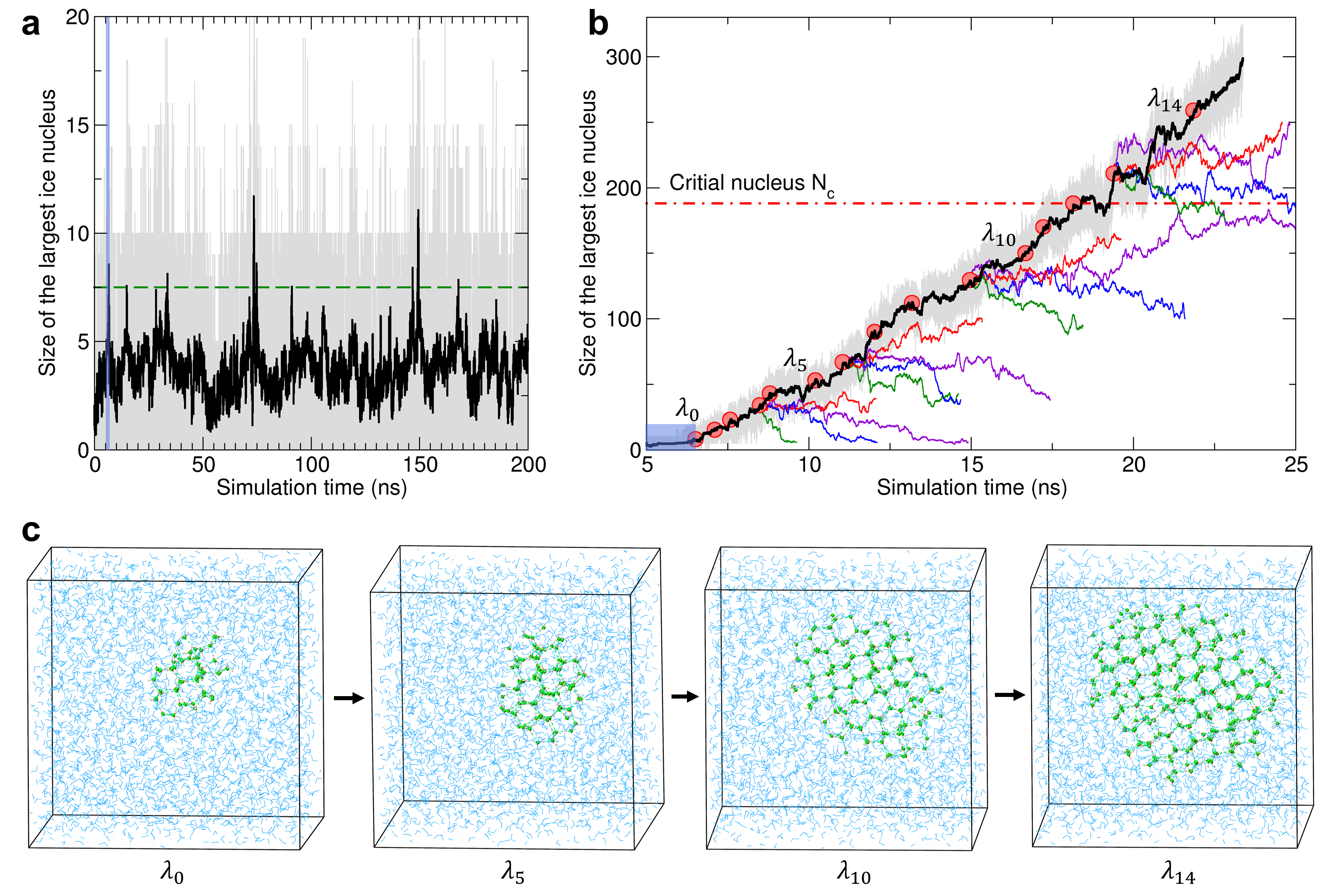
Fig. 1 presents the evolution of the largest ice nucleus size throughout the obtained trajectories. Within the 200 ns trajectory shown in Fig. 1a, no nucleation event is observed. In fact, simulating one nucleation event is expected to take approximately 0.1 s under the considered supercooling condition, which is far beyond the available temporal scale (typically $10^{-6}$ s) of MD simulations. However, several precritical ice nuclei with an instantaneous size of over 15 molecules form. The key is how to nurture such nuclei to larger ones exceeding the critical size to obtain a successful nucleation event. We choose the forward flux sampling (FFS)[13] method to overcome the time-scale limit of atomic simulations. In the FFS approach, a collective variable (CV) defined as the largest ice nucleus size (molecule number) is monitored during the MD simulations. The nucleation procedure is divided into multiple stages by milestones that are defined by a list of monotonously increasing CV values $\{\lambda_{0},\lambda_{1},\dotsb,\lambda_{n}\}$. At each milestone, dozens to hundreds of MD simulations starting from multiple initial configurations are launched, and they all have a chance to reach the next milestone. In this manner, continuous pseudo-brute-force nucleation trajectories can be obtained from a total of 36 $\mu$s-long MD trajectories.

Fig. 1b plots a successful ice nucleation trajectory with the milestones highlighted by red dots. The initial configuration used at the first milestone has a nucleus of size 22 and comes from the trajectory in Fig. 1a. Several snapshots of different ice nuclei labelled $\lambda_{0}$, $\lambda_{5}$, $\lambda_{10}$, and $\lambda_{14}$ are presented in Fig. 1c, and are marked in Fig. 1b at the corresponding time. The ice nucleus is cubic (Ic) and hexagonal (Ih) stacking-disordered, which is consistent with previous experimental and theoretical observations[24, 25, 13, 26, 27, 28, 11]. Counterintuitively, the ice nucleus size shows a rugged and reversible fluctuating behaviour throughout the whole nucleation process. The ice nucleus size could change slightly in a relatively long term, i.e., over 1 ns. It can also grow or shrink dramatically by more than 20 molecules in a relatively short term, i.e., less than 100 ps, as demonstrated by the subtrajectories launched at each milestone in the FFS simulation (Fig. 1b).

Figure 2: Dominant role of IC molecules in ice formation accompanied by structural and dynamical heterogeneity.  a, The largest nucleus size of ice versus the simulation time of one trajectory obtained in the FFS approach. Two representative processes, marked by I and II, refer to the growth and shrinkage of the nucleus, respectively. b, The largest ice nucleus of the initial configuration used in a. A slab is cut out from the simulation box for detailed observation (the same for c and d). c, d, Snapshots of the growth (c) and shrinkage (d) processes in a. Blue molecules are ice detected by common neighbour analysis. Red molecules are HM molecules, and pink molecules have relatively low mobility. The regions wrapped by green surfaces are defined as HM regions. The instant of each snapshot has been marked in a with the corresponding capital letter. e, Correspondence between the HIC and HM regions. The regions wrapped by orange and green surfaces refer to the HIC and HM regions, respectively. The system illustrated here consists of 23040 water molecules. f, Effect function $A_{\mathrm{IC}\rightarrow D}(t)$ shows a strong correlation between imperfectly coordinated molecules near the nucleus surface and the change in nucleus. On the other hand, the negative effect shown by $A_{\overline{\mathrm{IC}}\rightarrow D}(t)$ indicates that PC molecules prevent the ice nucleus changes.

Role of imperfectly coordinated water molecules

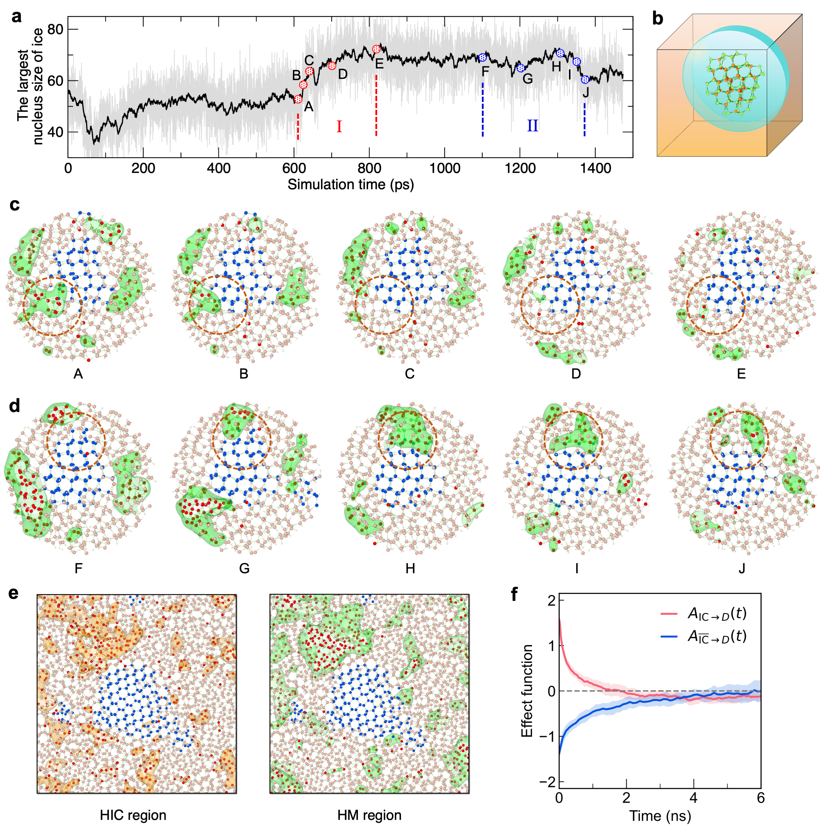
A visual inspection of the nucleation trajectories shows that the shape of the ice nucleus does not evolve in an isotropic manner; rather, some directions of the nucleus grow and shrink dramatically, while others remain unchanged in a relatively long term. Such dynamical anisotropic growth of ice nuclei might be connected with dynamical heterogeneity, a notable phenomenon of the coexistence of spatially distinguishable relatively mobile and immobile regions in supercooled water[29, 12]. The mobility of water molecules is contributed by the translational and rotational degrees of freedom. Here, we use a measure to quantify the translational and rotational mobility (see Methods section for the definition). A threshold corresponding to the top 10% of translational or rotational mobility in pure liquid water is set to distinguish the high-mobile (HM) molecules from others. The regions mainly composed of HM molecules are defined as HM regions. One representative trajectory in FFS involving both growth (process I) and shrinkage (process II) and the initial configuration are shown in Fig. 2a and 2b, respectively. In process I (Fig. 2c), the HM region located at the bottom left of the nucleus in snapshot A transforms to ice in snapshot E, with the gradual depletion of HM molecules. In process II (Fig. 2d), from snapshots F to H, an HM region near the top surface of the nucleus gradually expands to the ice nucleus and subsequently crushes the ordered H-bond network into a disordered state in snapshots I and J. These results illustrate that the HM regions act on ice nucleation by prominent rearrangement of the H-bond network. Significantly, the HM region does not necessarily introduce growth or melting of ice nucleus. For example, in process II (Fig. 2d), the bottom left surface of the nucleus remains unchanged, although it is adjacent to an HM region, the H-bond network in this area has gone through dramatic reconstruction. In contrast, other areas in processes I and II that are not part of or adjacent to the HM regions remain almost unchanged.

To understand the ice nucleation process from a structural perspective, we refer to the molecules forming four H-bonds, two accepting and two donating, with neighbouring molecules as perfectly coordinated (PC) molecules, and other molecules as imperfectly coordinated (IC) molecules. That is to say, an IC molecule can be viewed as carrying an IC status. We measure the probability of molecules with IC status in a given time window and define the one with a high IC status probability as an HIC molecule. Similar to the HM region, the HIC region can also be defined. See the Methods section for the details of these definitions. As shown in the left panel of Fig. 2e, the HIC region is spatially distinguishable from the remainder, indicating a structural heterogeneity behaviour, in accord with previous observations of the supercooled water structure[4, 7, 5]. In the right panel of Fig. 2e, we highlight the HM regions and find an almost perfect agreement with the HIC regions. To further investigate the correspondence of structural and dynamical heterogeneity, we calculate the cumulative distribution function of the translational and rotational mobility of molecules. A strong correlation between the coordination status of water molecules and their mobility is shown, i.e., most IC molecules exhibit higher mobility than PC molecules, in agreement with previous work[29, 30]. The time correlation function between HIC and HM molecules reveals a strong correlation.

From the discussion above, we can see that the role of the HIC regions in nucleus evolution is similar to that of the HM region, mainly due to the correspondence between structural and dynamical heterogeneity, resulting in the anisotropic growth or shrinkage of the ice nucleus. We further demonstrate the effect of HIC molecules on the nucleus by computing the effect function $A_{\textrm{IC}\rightarrow D}(t)$, defined by a net time-correlation between the appearance of IC molecules near the nucleus surface and the size change in the ice nucleus (see Methods for more details). From Fig. 2f, a positive effect with a typical decay time of $\sim 1.5$ ns is observed. These results imply that the IC molecules, only 4.88% of all molecules, act as engines to stimulate the HM region in supercooled water, drive the H-bond network rearrangement, and change the size of the ice nucleus. On the other hand, the effect of a PC H-bond environment (no IC molecule in the neighbourhood of a PC molecule) on the nucleus size change is investigated by the effect function $A_{\overline{\textrm{IC}}\rightarrow D}(t)$. A clear negative effect with a decay time of $\sim$4 ns proves that the H-bond network formed by PC molecules prevents the nucleus from growing or vanishing.

It should be emphasized that such a role of IC molecules does not intend to pilot the structure a priori to either the liquid or solid phase, which means that this is a “dual role” effect, and ice nucleation proceeds through competition and cooperation between IC and PC molecules. When IC molecules drive growth or shrinkage in some parts of the nucleus, the H-bond network formed by PC molecules prohibits the nucleus from melting or growing in the directions where the IC molecules are scarce or absent. This conclusion is different from the previous observations that ice was believed to be born in low mobile regions of supercooled water[12], in which the abundance and persistence of the tetrahedrally coordinated water molecules act as the precursor structure of ice nucleation[6, 7, 8, 9, 10, 11]. The hidden side of the microscopic picture of ice nucleation is that PC molecules alone cannot nurse disordered water into crystalline ice, but IC molecules play the decisive role of paving the pathway to ice formation. Our findings still hold if one traces back to the very beginning of nucleation that ice is born in high-mobile and low-mobile coexisting regions.

Figure 3: Microscopic mechanisms for H-bond network rearrangement during ice formation. Three representative ice growth events occur when one or several six-membered rings are constructed. a, Ice growth through IC status transfer. IC molecule W^∗ acts like a “catalyst” that induces the transfer of the imperfectly coordinated status among different molecules, facilitating the formation of six-membered rings around it. b, Ice growth through IC status transfer and annihilation. The IC molecule W^a first transfers its undercoordinate status to W^c, and then this IC status annihilates with the overcoordinated status of molecule W^e, resulting in two PC molecules. c, Ice growth through IC status generation and transfer. Two PC molecules W^a and W^c lean close to each other and turn into IC molecules. Then, W^b drifts away from W^a and W^b, recovering two PC molecules and leaving one IC status on itself. Specific water molecules are indexed with letters. The coordination number of IC molecules is marked with green numbers. Snapshots before and after the process are given, in which IC and PC molecules are coloured in green and pink, respectively, ice-like molecules are coloured in blue, and hydrogen atoms are in light grey.

Microscopic mechanism of H-bond network rearrangement

To induce ice formation, water molecules must reorient markedly and break at least the H-bond involving the rotating hydrogen. In order to get a deeper insight into the role of IC molecules during ice formation, we, therefore, monitor the ice growth or shrinkage events, in which the six-membered rings of the ice nucleus that follow the Bernal-Fowler ice rule[31] are formed or broken.

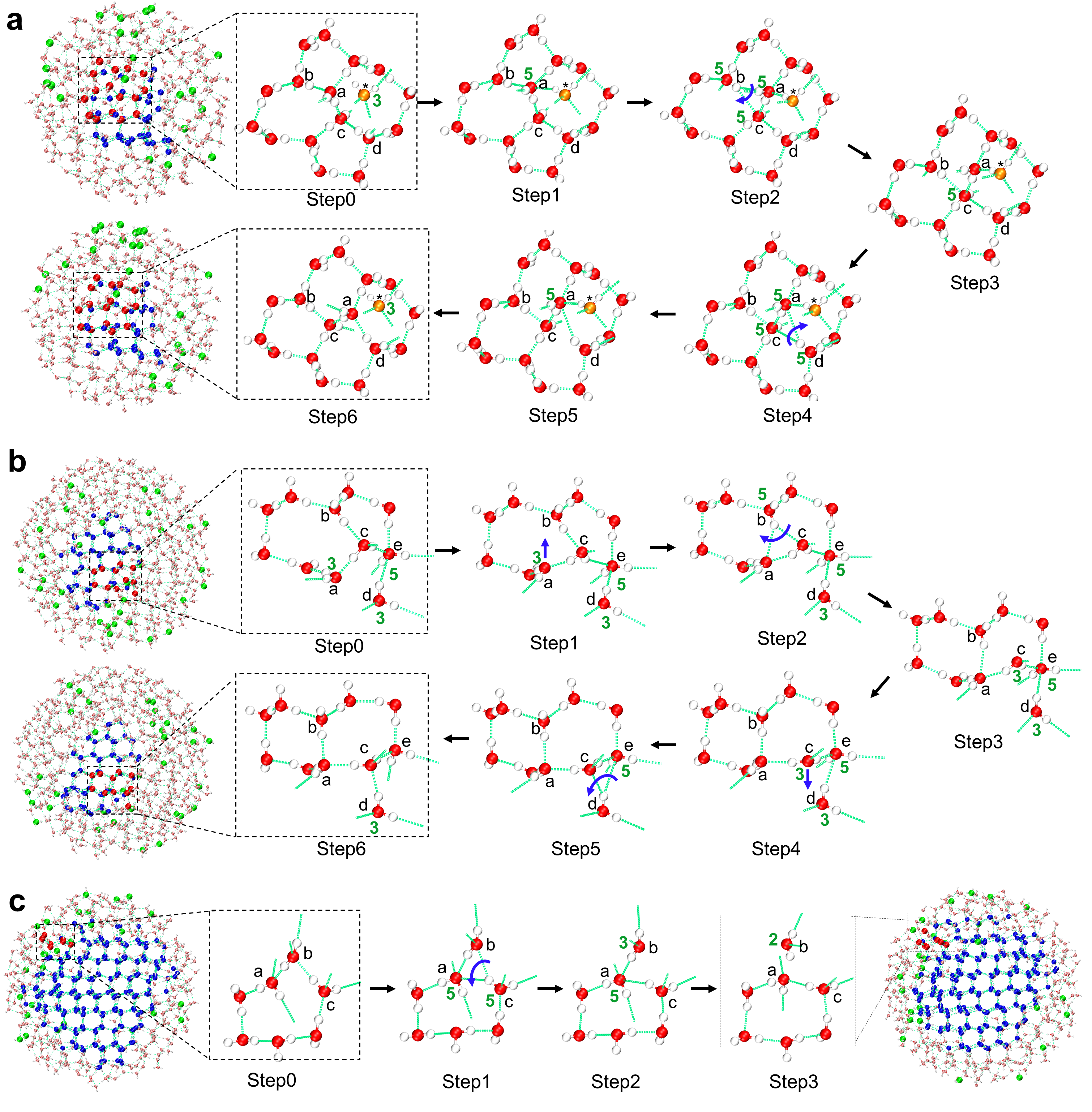
Fig. 3 presents three typical events that show the microscopic mechanism of how disordered water transforms into ordered ice. In the following description, W with superscript denotes a specified water molecule. As shown in Fig. 3a, in Step 0, pairs of five- and seven-membered rings are composed of 16 PC molecules. One IC molecule, W^∗, with three coordinations lies above these molecules. The W^∗ first moves towards W^a and forms a new H-bond with W^a (Step 1). Now, the W^∗ recovers the PC status, and W^a is overcoordinated. The H-bond from W^b to W^a oscillates until it bifurcates to form a new H-bond donated to W^c (Step 2). After that, W^b reorients, and the H-bond between W^a and W^b breaks (Step 3). The bifurcated H-bonds lower the activation energy of the H-bond network rearrangement from Steps 1 to 3 because the interaction energy of a bifurcated H-bond is roughly half of a linear bond[32]. As a consequence, W^c becomes overcoordinated. In a similar procedure, the H-bond from W^d to W^c bifurcates to form a new H-bond to W^a (Step 4), and then it breaks (Step 5). Eventually, the five-coordinated molecule W^a loses the H-bond with W^∗, and W^∗ returns to its initial three-coordinated status (Step 6). Reviewing the whole process, one can find that it starts with the presence of the IC molecule W^∗, which acts as a “catalyst”. Such a catalysing molecule can be viewed as carrying one active defect, i.e., an IC status. In this case, the IC status transfer follows a W^∗ $\rightarrow$ W^a $\xrightarrow{\text{W${}^{b}$}}$W^c $\xrightarrow{\text{W${}^{d}$}}$W^a $\rightarrow$ W^∗ path, in which W^b and W^d act as bridges. At the very end, the two pairs of five- and seven-membered rings transform into four six-membered rings, resulting in a bigger ice nucleus.

Along with the nucleus size increasing, the liquid region shrinks in the simulation box. Therefore, the concentration of IC molecules in the liquid region should increase since the IC status never dissipates according to the IC status transfer mechanism discussed above. However, our analysis shows that the concentration of IC molecules maintains dynamical equilibrium in the liquid region, indicating the annihilation and generation of IC status in supercooled water. We find that ice formation events can occur through IC status annihilation or generation since such phenomena also lead to H-bond network rearrangement. Fig. 3b presents a typical event involving the annihilation of IC statuses carried by two IC molecules. The IC status initially carried by W^a transfers to W^c (Steps 0 to 3). Then, the three-coordinated status of W^c and five-coordinated status of W^e annihilate, resulting in two PC molecules, and finally, the initial pair of five- and seven-membered rings transforms into two six-membered rings (Steps 4 to 6).

In contrast, Fig. 3c presents an ice formation event that is induced by IC status generation. Here, molecule W^a, situated in the second neighbour shell of molecule W^c, fluctuates and occasionally moves near W^c, leading to the bifurcation of the H-bond donated from W^c to W^a and W^b (Step 0 to 1). Subsequently, the H-bond from W^c to W^b breaks, and a pair of three- and five-coordinated molecules is generated (Step 2). Finally, the H-bond between W^a and W^b breaks, W^a becomes PC, while W^b changes to a two-coordinated status (Step 3). This event leads a seven-membered ring to a six-membered ring.

By analyzing all the ice formation events throughout the whole ice nucleation trajectory in Fig. 1b, we find that the H-bond network rearrangements are realized by three mechanisms, i.e., IC status transfer, annihilation, and generation, resulting in transformations between disordered and ordered states. Among the three microscopic mechanisms, IC status transfer is the dominant player, approximately 90% of the growth events rely on it. In addition, events of ice nucleus shrinkage follow the same mechanisms in our observation. We find that the transfer process of IC status is different from the molecular jump mechanism of water reorientation reported in the supercooled water[33]; i.e., the rotating water molecule breaks an H-bond with an overcoordinated first-shell neighbour and forms an H-bond with an undercoordinated second-shell neighbour. From our observations, in many cases, the reorientation and H-bond cleavage/formation can occur with the existence of a single IC molecule. It is worth noting that the ice nucleation microscopic mechanism presented here is also valid in the TIP4P/ice water model.

Figure 4: Homogeneous ice nucleation rate and free energy surface. a, Ice nucleation rate dependent on the degree of supercooling, with the ordinate logarithmically scaled based on 10. The data include the results obtained in this work and some previous theoretical[34, 35, 36, 37, 38, 13, 11, 39] and experimental[40, 41, 42, 43, 44, 45, 46, 47, 48, 49] work. Experimental results are marked by crosses or asterisks with the legend located in the upper left of the figure and theoretical results are solid polygons or dashed lines with the legend in the lower right. The yellow shadow region is drawn only to guide the eyes. b, Free energy surface constructed by umbrella sampling as a function of the number of ice-like molecules $N_{i}$, which is identified by the environment similarity metric[50]. The error bar is presented by the light-blue zone, as shown in b. c, Free energy surface constructed by reweighting the umbrella sampling data to the axis of the size of the largest ice nucleus, the same collective variable as in Fig. 1. The red dashed line is obtained by fitting the free energy curve using the function $f(n)=an^{2/3}+bn+c$ given from the classical nucleation theory, where $a=3.200$ and $c=-7.475$ are obtained by approximating the blue curve, and $b$ is the chemical potential difference between the solid and liquid phases equal to $-0.376$ $k_{B}T$, which is calculated by thermal integration.

Ice nucleation rate

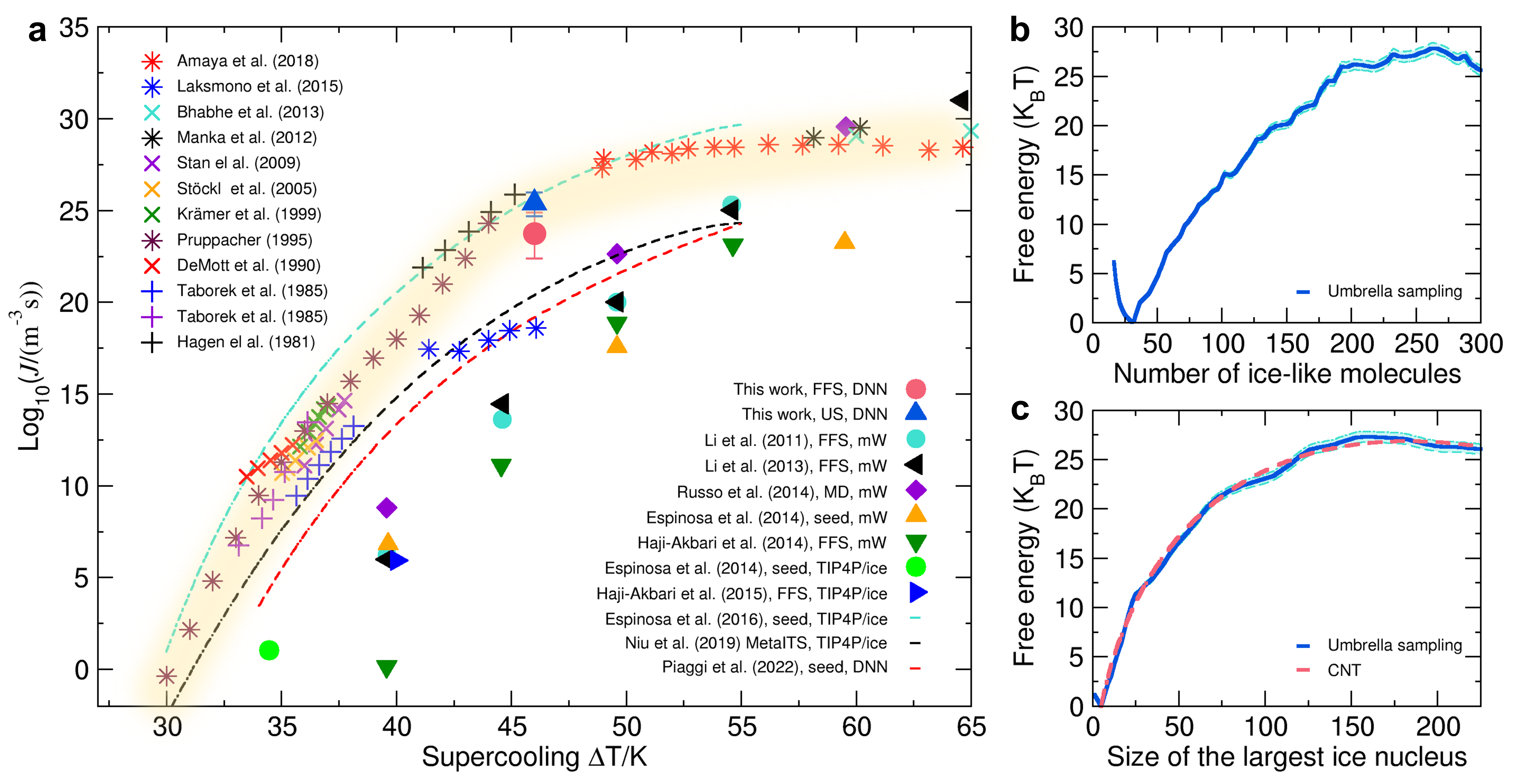
Accurately estimating the ice nucleation rate under homogeneous conditions is another challenge for both experiments and computer simulations[13]. As shown in Fig. 4a, most experimental results[40, 41, 42, 43, 44, 45, 46, 47, 48, 49] fall into the yellow shadow region, while the theoretical results[34, 35, 36, 37, 38, 13, 11, 39] are rather scattered. Among all the theoretical techniques used to calculate the ice nucleation rate, the FFS method is known to be rigorous since it can calculate the rate directly. In this work, through the FFS method[13], we obtain that the ice nucleation rate in logarithm is $\log_{10}J=23.70^{+1.18}_{-1.32}$ ($J$ in $m^{-3}\cdotp s^{-1}$) and the critical nucleus size is $188$ at a supercooling of 46 K. To validate the result obtained by the FFS method, we further use the umbrella sampling method[51] to calculate the free energy surface (FES, shown in Fig. 4b) along the nucleation path as a function of the ice-like molecule number, identified by the environment similarity metric[50]. Then, we reweight this FES to the CV of the largest ice nucleus size and obtain Fig. 4c. The red dashed line in Fig. 4c is the fitting curve using the classical nucleation theory (CNT). The homogeneous ice nucleation process conforms to the CNT reasonably well. The critical size and the energy barrier obtained by the CNT fitting are $183^{+8}_{-8}$ and $26.85^{+1.45}_{-1.26}$ $k_{B}T$, respectively. Eventually, the logarithm of the nucleation rate is $\log_{10}J=25.35^{+0.62}_{-0.68}$ ($J$ in $m^{-3}\cdotp s^{-1}$), which is consistent with the rate calculated by the FFS method, indicating the faithfulness of our estimation with both methods. The excellent agreement between our results and experiments substantiates the accuracy of the water model and the reliability of the ice nucleation microscopic mechanism proposed here.

Summary

To summarize, we report MD simulation trajectories of ice nucleation under homogeneous conditions with the DNN water model that reaches ab initio accuracy. We find that the IC molecules play a decisive role in ice nucleation in the sense that they pave the way between the disordered liquid state and the ordered solid state, and that the PC H-bond network preserves the existing ice nucleus from either growing or melting. Ice is born under competition and cooperation between the IC and PC molecules. Additionally, the nucleation process is well described by the CNT, and the nucleation rates estimated by this work are in excellent agreement with the experimental records. We expect that the relationship between IC molecules and nucleation in water provides new but important insight into the phase transition process and other complex behaviours of water. For other dynamic processes, such as heterogeneous ice nucleation, nucleation in water solution, and anti-freezing proteins, the effect of IC molecules should not be neglected.

Methods

Simulation programs and settings

All molecular dynamics simulations are calculated on Lammps[52], integrated with DeePMD-kit[53] used to simulate with the deep neural network potential. The simulation system is in an orthorhombic box with periodic boundary conditions in all three directions, which consists of 2880 water molecules unless otherwise specified. The time interval of the integral of motion, i.e., time step, is set to 0.5 fs. Temperature and pressure are controlled by Nosé-Hoover style thermostat and barostat, set to 265 K relaxed per 1 ps and 1 bar relaxed per 0.05 ps, respectively. Such temperature refers to a supercooling 46 K of the DNN model. Each particle starts with an initial velocity following the Maxwell-Boltzmann distribution and generated by a random seed. In order to prevent the uniform rectilinear motion of the whole system, the linear momentum of each atom is rescaled by subtracting the momentum of centre of mass every 1000 time steps. As for umbrella sampling and ice structure identification, Plumed 2[54] is interfaced with Lammps so as to bias or analyse the trajectories. Crystal structure visualization is implemented by Ovito[55] and Vmd[56].

Generation of the deep neural network (DNN) model

The training of the DNN model is performed on the software package DeePMD-kit. The settings of training parameters are as follows: the size of the embedding net and fitting net are respectively (10,20,40) and (240,240,240). The cut-off radius is 6 Å. The smoothing parameter rcut_smth is set to 0.5 Å. In each training step, a minibatch, i.e., a small subset of the training dataset, is served to evaluate the gradient of the loss function. The hyper-parameters start_pref_e, start_pref_f, start_pref_v, limit_pref_e, limit_pref_f and limit_pref_v that control the weights of energy and force losses in the total loss function are set to 0.02, 1000, 0.05, 2.0, 1.0, and 0.5, respectively. The starting learning rate is 0.002 and exponentially decays to $2\times 10^{-8}$ at the end of the training. The total training steps are set to $1\times 10^{7}$.

To build the DNN model applicable to water nucleation, our model has gone through an iterative update for better performance. The first generation of the DNN model is generated using the liquid configurations at standard temperature and pressure and all the experimentally known stable or metastable ice polymorphs for P $\lesssim$ 50 GPa (including phases of Ih, Ic, II, III, IV, V, VI, VII, VIII, IX, XI, XII, XIII, XIV, XV). The total size of the dataset is 28097. All the above configurations are taken from Ref[18]. However, such a dataset does not contain the solid-liquid coexistence configurations, which leads to insufficient accuracy of the potential energy predictions during the nucleation process. Therefore, we run metadynamics[57] simulations using the first generation of DNN potential, with a combination of the intensities of several structural factor peaks chosen as the collective variable[11]. In this way, 3734 new configurations consisting of liquid-Ic, liquid-Ih and liquid-Isd coexisting regions are added to the dataset, which is used to train the new generation of the DNN model that is used in this work.

Forward flux sampling

Forward flux sampling (FFS)[13, 58] is a path sampling strategy in order to sample rare events dependent on a specified CV $\lambda$. Here, the whole nucleation process is divided into multiple stages. Each stage is marked by a certain value of CV. Thereby a monotonous sequence $\{\lambda_{0},\lambda_{1},\dotsb,\lambda_{n}\}$ is established as “milestones” to assess the progress of the reaction. The initial state (pure liquid) is separated by $\lambda\leq\lambda_{l}$, where $\lambda_{l}=5$ is the smallest nucleus size that can be detected by the common neighbour analysis. Additionally, this value also corresponds to the lowest point on the free energy surface shown in Fig. 4b. The main task of FFS is to estimate the probability for a trajectory starting from one milestone to reaching the next. The nucleation rate can be calculated by

$$R=\frac{\overline{\Phi}_{0}}{\overline{h}_{0}}\prod_{i=0}^{n-1}P(\lambda_{i+1}|\lambda_{i}),$$ (1)

in which $\overline{\Phi}_{0}/\overline{h}_{0}$ equals to the number of times of a long MD trajectory crossing $\lambda_{0}$ from $\lambda<\lambda_{l}$ divided by the length of simulation. $P(\lambda_{i+1}|\lambda_{i})$ is the transfer probability from milestone $\lambda_{i}$ to $\lambda_{i+1}$, estimated by performing a “shooting test” at $\lambda_{i}$, which means to launch plenty of trajectories starting at $\lambda_{i}$ and calculate the probability of a trajectory reaching $\lambda_{i+1}$ but not falling into $\lambda_{l}$. The error of $P(\lambda_{i+1}|\lambda_{i})$ for each $i$ is evaluated by the standard deviation of transfer probabilities obtained from different initial configurations, and such error will propagate to the subsequent milestones along with Eq. (1).

Umbrella sampling

Umbrella sampling[51] is one of the oldest but most versatile enhanced sampling methods based on free energy theory. In this method, the whole nucleation process is divided into multiple sections called “windows”. The sampling is carried out on each window respectively. At last, merge the sampling data from each window and subsequently obtain the global free energy surface (FES). The sampling on each window is implemented by a long MD simulation that exerted an extra quadratic restraint. The restraint added on sampling window $i$ can be written as

$$V_{i}=\frac{1}{2}K(s-s_{i})^{2},$$ (2)

where $s$ is the CV, $s_{i}$ represents the centre of the $i$-th window, $K$ is a constant set to 1 kJ/mol. The CV refers to the number of ice-like molecules, identified by the environment similarity metric. In total, 60 runs are performed to cover the CV space ranging from 20 to 315 with an interval of 5. For each run, a total of 16 ns simulation is performed. We use the weighted histogram analysis method (WHAM)[59, 60] to reweight the data and construct the FES. Eventually, a converged FES is obtained.

Ice structure identification and collective variables

In this work, two methods are adopted to identify whether a water molecule is an ice molecule or not. For the process of FFS, the CV is chosen as the size of the largest nucleus (molecule number). To estimate it, an extended version of common neighbour analysis (CNA)[16] method is employed. This method takes the second nearest neighbours into consideration to discriminate the structures of cubic diamond and hexagonal diamond. In practice, only oxygen atoms are considered and in this way, each water molecule can be identified as Ih, Ic or others. If a molecule is judged to be either Ih or Ic structure, its 4 nearest and itself are regarded as ice molecules. At the very end, a graph is established that each ice molecule links to its 4 nearest vertices, and the largest nucleus corresponds to the maximum connected component of the system. In order to reduce the computational costs, the calculation of the largest nucleus size is performed every 200 time steps, i.e., 0.1 ps. Additionally, for convenient illustration, the nucleus size highlighted in all the snapshots includes the second shell of the central molecule.

However, this absolute ice nucleus size is non-differentiable and thereby cannot be used in biased molecular dynamical simulations. Hence, in the umbrella sampling, we adopt the environment similarity metric introduced by Piaggi et al.[50] which is based on the methodology of smooth overlap of atomic position (SOAP)[61]. This CV first compares the configuration $\omega$ presenting the the environment of a central atom within a certain cut-off radius respectively to each given configuration in the reference set $X=\left\{\chi_{1},\chi_{2},\dotsb,\chi_{n}\right\}$. In this work, only oxygen atoms are considered and $X$ consists of 8 configurations that can completely describe the structure of Ih, Ic and Isd. The similarity between $\omega$ and $\chi_{k}$ is calculated by

$$k_{\chi_{k}}(\omega)=\frac{1}{N_{k}}\sum_{i\in\omega}\sum_{j\in\chi_{k}}\exp\left(-\frac{\lVert\bm{r}_{i}-\bm{r}_{j}\rVert^{2}}{4\sigma^{2}}\right),$$ (3)

where $N_{k}$ is the atom number in configuration $\chi_{k}$, $\bm{r}_{i}$ and $\bm{r}_{j}$ are the position vector pertaining to the configuration $\omega$ and $\chi_{k}$ respectively with the origin located on the central atom. $\sigma$ is the width of Gaussian aimed to limit the deviation relative to the reference configuration. Here, we set $\sigma$ to 0.055. Next, $k_{X}(\omega)=\max\limits_{\chi_{k}\in X}k_{\chi_{k}}(\omega)$ is defined as the similarity metric compared to the reference set $X$. If $k_{X}(\omega)$ is larger than a certain value, we say the central atom is “ice-like”. The CV used in umbrella sampling in this work is the number of ice-like atoms in the whole system. In practice, this value is calculated using a soft threshold by

$$s=\sum_{i}\left(1-w(k_{X}(\omega_{i}))\right),$$ (4)

where $s$ denotes the calculated CV, $\omega_{i}$ is the environment of atom $i$. The summation is applied to all oxygen atoms in the system. $w(\cdot)$ is the switching function with the form of rational type

$$w(x)=\frac{1-(x/x_{0})^{12}}{1-(x/x_{0})^{24}}.$$ (5)

This function will decay from 1 smoothly to zero as $x$ increases. $x_{0}$ is set to 0.55 in this work.

Data smoothing

Grey lines in Fig. 1 and Fig. 2 show the instantaneous value of max nucleus size calculated by CNA, exhibiting violent fluctuation in a relatively short term during the whole simulation. To obtain a relatively stable largest nucleus size, we calculate the exponential moving average (EMA) by

$$S_{t}^{EMA}=\begin{cases}S_{t}&t=0;\\ \alpha S_{t}+(1-\alpha)S_{t-1}^{EMA}&t>0,\end{cases}$$ (6)

where $S_{t}$ is the instantaneous value at $t$, $\alpha$ is a constant and set to $2/501$ in this work. The EMA makes the smoothed data as close as possible to the original data but the fluctuations are greatly alleviated. We confirm this treatment to be reasonable since any changes in the largest nucleus size can be detected accurately by the smoothed data.

As for the analysis of the ice formation mechanism in Fig. 3, the trajectory is smoothed by computing the average of the coordinates over a time window centred at the current time. It is worth noting that the choice of the smoothing window size and the time interval between frames should not be too large to lose the concrete process of the H-bond reconstruction event. In this work, the trajectory is dumped every 10 fs, and the smoothing window size is set to 20 frames.

Measure of dynamical behaviours

Dynamic behaviours of water molecules discussed in this work consist of two parts: translation and rotation. For the translation behaviour of molecule $i$ at time $t$, we use $\langle\lVert\Delta\bm{r}_{i}(t)\rVert^{2}\rangle$ as an estimator. Here, the average $\langle\cdot\rangle$ is taken over a given time window $t$ to $t+T$. More concretely, it can be written in discrete form by

$$\langle\lVert\Delta\bm{r}_{i}(t)\rVert^{2}\rangle=\frac{1}{T}\sum_{\tau}^{T}\lVert\bm{r}_{i}(t+\tau)-\bm{r}_{i}(t)\rVert^{2},$$ (7)

where $\bm{r}_{i}(t)$ and $\bm{r}_{i}(t+\tau)$ is the position of oxygen atom of molecule $i$ at the present time $t$ and the time after $\tau$, respectively.

As for rotation, the definition of the estimator is similar to translation in Eq. (7). We start by the calculations of the rotation vectors using the method in Ref[29] by Mazza et al. To measure the three independent degrees of freedom of the rotation, we set three mutually perpendicular axes on each molecule $i$ with the origin located at the oxygen atom. The unit vectors of these three axes are named $\bm{p}_{i}^{1}$, $\bm{p}_{i}^{2}$ and $\bm{p}_{i}^{3}$, respectively. $\bm{p}_{i}^{1}$ denotes the angular bisector of two O-H bonds. $\bm{p}_{i}^{2}$ is normal to the H-O-H plane. $\bm{p}_{i}^{3}$ directs to the cross product of $\bm{p}_{i}^{1}$ and $\bm{p}_{i}^{2}$. Next, $\delta\bm{\varphi}_{i}^{j}(t)$ is defined to evaluate the rotation of molecule $i$ around axis $j$ between time $t$ and $t+\Delta t$, which is calculated by

$$\delta\bm{\varphi}_{i}^{j}(t)=\cos^{-1}\left[\bm{p}_{i}^{j}(t)\cdot\bm{p}_{i}^{j}(t+\Delta t)\right]\frac{\bm{p}_{i}^{j}(t)\times\bm{p}_{i}^{j}(t+\Delta t)}{\lVert\bm{p}_{i}^{j}(t)\times\bm{p}_{i}^{j}(t+\Delta t)\rVert}.$$ (8)

This means the modulus of $\delta\bm{\varphi}_{i}^{j}(t)$ is equal to the size of rotation angle and the direction is normal to the rotation plane. Then $\bm{\varphi}_{i}^{j}(t)$ is calculated as

$$\bm{\varphi}_{i}^{j}(t)=\sum_{\tau}^{t}\delta\bm{\varphi}_{i}^{j}(\tau).$$ (9)

Then, $\langle\lVert\Delta\bm{\varphi}_{i}^{j}(t)\rVert^{2}\rangle$ is calculated likewise by taking average over the time window $t$ to $t+T$, i.e.,

$$\langle\lVert\Delta\bm{\varphi}_{i}^{j}(t)\rVert^{2}\rangle=\frac{1}{T}\sum_{\tau}^{T}\lVert\bm{\varphi}_{i}^{j}(t+\tau)-\bm{\varphi}_{i}^{j}(t)\rVert^{2}.$$ (10)

We use the sum of $\langle\lVert\Delta\bm{\varphi}_{i}^{1}(t)\rVert^{2}\rangle$, $\langle\lVert\Delta\bm{\varphi}_{i}^{2}(t)\rVert^{2}\rangle$ and $\langle\lVert\Delta\bm{\varphi}_{i}^{3}(t)\rVert^{2}\rangle$ to estimate the rotation behaviour of molecule $i$.

The length of time $T$ in Eq. (7) and (10) should be set manually. In this work, $T$ is set to 100 ps. This choice is comparable with the length of the half-life decay time of $A_{\text{IC}\rightarrow D}(t)$ shown in Fig. 2f in the main text.

High mobile regions

The definition of the high-mobile (HM) region is based on HM molecules. To determine whether a molecule is HM or not, we first simulate pure liquid water and calculate the distribution of the translational and rotational mobility over all molecules of all frames. The threshold of high mobility is corresponding to the highest 10% mobile molecules. At supercooling 46 K, the values for translation and rotation are 7.7 Ų/ps and 12.8 rad²/ps, respectively. We define that a molecule as HM if it has either of two types of mobility above the respective threshold. Then, smearing normalized three-dimensional Gaussian density function on each HM molecule, any position in the simulation box will take a value by the summation of all added functions. The region wrapped by an isosurface is defined as the HM region. In this work, the width of Gaussian is set to 1.73 Å, and the isovalue is set to 1.

IC status probability

To better explain the relationship between the IC status and mobility, we introduce the measure of the IC status probability. For each water molecule, its value is calculated as the frequency of the molecule being in IC status in a time window centred at the current time. The size of the time window is set to 100 ps, the same as the definition of the measure of mobility. To make this measure comparable with HM regions, we first calculate the fraction of HM molecules in liquid water at supercooling 46 K. The threshold for high IC status probability (HIC) is set so that the fraction of HIC molecules is the same as the fraction of HM molecules. We obtain the threshold value for HIC is 9.79%. The region of the HIC in Fig. 2 is plotted through the same method as the HM region but the Gaussian is smearing on the HIC molecules.

Effect function

To investigate the effect of the imperfectly coordinated (IC) water molecules on the size change of the ice nucleus, we define the effect function $A_{\mathrm{IC}\rightarrow D}(t)$ as the difference between the following two time correlation functions:

$$A_{\textrm{IC}\rightarrow D}(t)=C_{(N_{\textrm{IC}}\cap S),D}(t)-C_{S,D}(t),$$ (11)

where the time correlation functions are defined by

$$C_{N_{\textrm{IC}}\cap S,D}(t) =\frac{\big{\langle}N_{\textrm{IC}}^{i}(T)\cdot S^{i}(T)\cdot D^{i}(T+t)\big{\rangle}_{i,T}}{{\langle N^{i}_{\textrm{IC}}(T)S^{i}(T)\rangle_{i,T}\langle D^{i}(T)\rangle_{i,T}}},$$ (12)

$$C_{S,D}(t) =\frac{\big{\langle}S^{i}(T)\cdot D^{i}(T+t)\big{\rangle}_{i,T}}{\langle S^{i}(T)\rangle_{i,T}\langle D^{i}(T)\rangle_{i,T}}.$$ (13)

In Eqs. (12) and (13), $N_{\textrm{IC}}^{i}(T)$ denotes the number of IC molecules in the neighbourhood $\mathcal{N}(i)$ of molecule $i$; $S$ and $D$ are indicator functions (definition introduced later) telling if molecule $i$ is near the nucleus surface and if its status (ice or water) changes, respectively; the average $\langle\cdot\rangle_{i,T}$ is taken over the molecular index $i$ and the simulation time $T$. The $C_{S,D}$ denotes the time-correlation function between indicators $S$ and $D$, while $C_{(N_{\textrm{IC}}\cap S),D}$ is the time-correlation function between an indicator function telling if a near-nucleus-surface water molecule has IC molecules in its neighbourhood (denoted by $N_{\textrm{IC}}\cap S$) and the indicator function $D$.

To properly define the indicators, we introduce a status function $I^{i}(T)$ that takes the value of 1 if the molecule $i$ is belonging to an ice nucleus at time $T$, otherwise takes a value 0. The surface indicator $S^{i}(T)$ is defined by the standard deviation of the status function in the neighbourhood of molecule $i$, i.e.,

$$S^{i}(T)=\textrm{std}\big{(}I^{j}(T)\big{)}_{j\in\mathcal{N}(i)}.$$ (14)

It is clear that if the molecule is inside the water or ice region, all the status function $I^{j}$ respectively takes value 0 or 1, so the standard deviation vanishes. On the other hand, if the molecule is near the surface, then there must be some ice and water molecules co-existing in the neighbourhood, which leads to a non-zero surface indicator. The time-dependent functions $N_{\textrm{IC}}^{i}(T)$ and $S^{i}(T)$ are smoothed along the trajectories with a window size of 40 ps.

The change-of-status indicator is defined as the difference between the status function of two consecutive times along the trajectory separated by a time resolution $\tau$, i.e.

$$D^{i}(T)=|I^{i}(T+\tau)-I^{i}(T)|$$ (15)

The indicator function takes the absolute value of the difference in $I^{i}$ to take into consideration both the water-to-ice and ice-to-water changes. The indicator function $I^{i}(T)$ is smoothed along the trajectories with a window size of 40 ps.

Similar to the effect function $A_{\textrm{IC}\rightarrow D}(t)$, we define $A_{\overline{\textrm{IC}}\rightarrow D}(t)$ quantifying the effect of a PC environment (no IC molecule presents in the neighborhood of a molecule) and the change of the status of a molecule.

$$A_{\overline{\textrm{IC}}\rightarrow D}(t)=C_{(\overline{N}_{\textrm{IC}}\cap S),D}(t)-C_{S,D}(t),$$ (16)

where $\overline{N}^{i}_{\textrm{IC}}$ is defined by

$$\overline{N}^{i}_{\textrm{IC}}(T)=\left\{\begin{aligned} 1\quad&\textrm{if}\ N^{i}_{\textrm{IC}}(T)=0;\\ 0\quad&\textrm{otherwise}.\end{aligned}\right.$$ (17)

Calculation of nucleation rate based on classical nucleation theory

Using the FFS method one can obtain nucleation rate directly, but the umbrella sampling can not. Through the umbrella sampling the nucleation barrier $\Delta G^{*}$ is obtained. The classical nucleation theory (CNT)[62] predicts the nucleation rate $J$ as

$$J=\rho_{l}Zf^{+}\exp\left(-\frac{\Delta G^{*}}{k_{B}T}\right),$$ (18)

where $\rho_{l}$ is the number density of liquid, $Z$ is the Zeldovich factor, $k_{B}$ is the Boltzmann constant, $T$ is the temperature, $f^{+}$ is the attachment rate describing the diffusion behaviour near the critical nucleus size. The Zeldovich factor can be calculated by

$$Z=\left[\frac{\Delta G^{*}}{3\pi k_{B}TN_{c}^{2}}\right]^{1/2},$$ (19)

where $N_{c}$ is the number of molecules when the nucleus is critical. This equation of the Zeldovich factor is applicable to various geometry shape of the nucleus, including ellipsoid. The attachment rate is calculated as the diffusion coefficient of the molecule number of the critical nucleus, written as

$$f^{+}=\frac{\langle(N(t)-N(0))^{2}\rangle}{2t},$$ (20)

where $\langle\cdot\rangle$ denotes the ensemble average and $N(t)$ is the molecule number of the nucleus at time $t$. Here, the attachment rate $f^{+}$ of water at supercooling 46 K is evaluated to be $3.4713\times 10^{10}$ s^-1.

Data availability

The main data supporting the findings of this study are available within the paper. Additional information and data are available from the corresponding author upon reasonable request.

Code availability

LAMMPS, Plumed, and DeePMD-kit are free and open source codes available at https://lammps.sandia.gov, https://www.plumed.org, and http://www.deepmd.org, respectively. Additional codes are available from the corresponding author upon reasonable request.

Author contributions

H.N. conceived the idea and designed the research. H.W. conceived the idea to sample the pseudo-brute-force ice nucleation trajectories. M.C., L.T. and H.N. carried out the FFS simulations and analyzed the data. M.C. and H.N. carried out the umbrella sampling simulations. L.T., H.N. trained the water DNN model with the help of H.W. and L.Z.. H.W. performed the effect function analysis. M.C. and H.W. wrote the codes for data analysis. The text was initially composed by M.C., H.N, and H.W. and all the authors contributed to the discussion of the research and the final version of the manuscript.

References

- Bartels-Rausch et al. [2012] Thorsten Bartels-Rausch, Vance Bergeron, Julyan HE Cartwright, Rafael Escribano, John L Finney, Hinrich Grothe, Pedro J Gutiérrez, Jari Haapala, Werner F Kuhs, Jan BC Pettersson, et al. Ice structures, patterns, and processes: A view across the icefields. Reviews of Modern Physics, 84(2):885, 2012.
- Bartels-Rausch [2013] Thorsten Bartels-Rausch. Chemistry: Ten things we need to know about ice and snow. Nature, 494(7435):27, 2013.
- Brini et al. [2017] Emiliano Brini, Christopher J Fennell, Marivi Fernandez-Serra, Barbara Hribar-Lee, Miha Luksic, and Ken A Dill. How water’s properties are encoded in its molecular structure and energies. Chemical Reviews, 117(19):12385–12414, 2017.
- Sellberg et al. [2014] Jonas A Sellberg, C Huang, Trevor A McQueen, ND Loh, H Laksmono, Daniel Schlesinger, RG Sierra, D Nordlund, CY Hampton, Dmitri Starodub, et al. Ultrafast X-ray probing of water structure below the homogeneous ice nucleation temperature. Nature, 510(7505):381, 2014.
- Gallo et al. [2016] Paola Gallo, Katrin Amann-Winkel, Charles Austen Angell, Mikhail Alexeevich Anisimov, Freédeéric Caupin, Charusita Chakravarty, Erik Lascaris, Thomas Loerting, Athanassios Zois Panagiotopoulos, John Russo, et al. Water: A tale of two liquids. Chemical Reviews, 116(13):7463–7500, 2016.
- Matsumoto et al. [2002] Masakazu Matsumoto, Shinji Saito, and Iwao Ohmine. Molecular dynamics simulation of the ice nucleation and growth process leading to water freezing. Nature, 416(6879):409, 2002.
- Tanaka [2012] Hajime Tanaka. Bond orientational order in liquids: Towards a unified description of water-like anomalies, liquid-liquid transition, glass transition, and crystallization. The European Physical Journal E, 35(10):113, 2012.
- Moore and Molinero [2011a] Emily B Moore and Valeria Molinero. Structural transformation in supercooled water controls the crystallization rate of ice. Nature, 479(7374):506, 2011a.
- Bullock and Molinero [2013] Griffin Bullock and Valeria Molinero. Low-density liquid water is the mother of ice: On the relation between mesostructure, thermodynamics and ice crystallization in solutions. Faraday Discussions, 167:371–388, 2013.
- Overduin and Patey [2015] SD Overduin and GN Patey. Fluctuations and local ice structure in model supercooled water. The Journal of Chemical Physics, 143(9):094504, 2015.
- Niu et al. [2019] Haiyang Niu, Yi Isaac Yang, and Michele Parrinello. Temperature dependence of homogeneous nucleation in ice. Physical Review Letters, 122(24):245501, 2019.
- Fitzner et al. [2019] Martin Fitzner, Gabriele C Sosso, Stephen J Cox, and Angelos Michaelides. Ice is born in low-mobility regions of supercooled liquid water. Proceedings of the National Academy of Sciences, 116(6):2009–2014, 2019.
- Haji-Akbari and Debenedetti [2015] Amir Haji-Akbari and Pablo G Debenedetti. Direct calculation of ice homogeneous nucleation rate for a molecular model of water. Proceedings of the National Academy of Sciences, 112(34):10582–10588, 2015.
- Sosso et al. [2016] Gabriele C. Sosso, Ji Chen, Stephen J. Cox, Martin Fitzner, Philipp Pedevilla, Andrea Zen, and Angelos Michaelides. Crystal nucleation in liquids: Open questions and future challenges in molecular dynamics simulations. Chemical Reviews, 116(12):7078–7116, June 2016. ISSN 0009-2665, 1520-6890. doi: 10.1021/acs.chemrev.5b00744.
- Kadaoluwa Pathirannahalage et al. [2021] Sachini P. Kadaoluwa Pathirannahalage, Nastaran Meftahi, Aaron Elbourne, Alessia C. G. Weiss, Chris F. McConville, Agilio Padua, David A. Winkler, Margarida Costa Gomes, Tamar L. Greaves, Tu C. Le, Quinn A. Besford, and Andrew J. Christofferson. Systematic comparison of the structural and dynamic properties of commonly used water models for molecular dynamics simulations. Journal of Chemical Information and Modeling, 61(9):4521–4536, September 2021. ISSN 1549-9596, 1549-960X. doi: 10.1021/acs.jcim.1c00794.
- Maras et al. [2016] E. Maras, O. Trushin, A. Stukowski, T. Ala-Nissila, and H. Jónsson. Global transition path search for dislocation formation in Ge on Si(001). Computer Physics Communications, 205:13–21, August 2016. ISSN 00104655. doi: 10.1016/j.cpc.2016.04.001.
- Chen et al. [2017] Mohan Chen, Hsin-Yu Ko, Richard C Remsing, Marcos F Calegari Andrade, Biswajit Santra, Zhaoru Sun, Annabella Selloni, Roberto Car, Michael L Klein, John P Perdew, et al. Ab initio theory and modeling of water. Proceedings of the National Academy of Sciences, 114(41):10846–10851, 2017.
- Zhang et al. [2021] Linfeng Zhang, Han Wang, Roberto Car, and E Weinan. Phase diagram of a deep potential water model. Physical Review Letters, 126(23):236001, 2021.
- Sun et al. [2015] Jianwei Sun, Adrienn Ruzsinszky, and John P Perdew. Strongly constrained and appropriately normed semilocal density functional. Physical Review Letters, 115(3):036402, 2015.
- Sun et al. [2016] Jianwei Sun, Richard C Remsing, Yubo Zhang, Zhaoru Sun, Adrienn Ruzsinszky, Haowei Peng, Zenghui Yang, Arpita Paul, Umesh Waghmare, Xifan Wu, et al. Accurate first-principles structures and energies of diversely bonded systems from an efficient density functional. Nature Chemistry, 8(9):831, 2016.
- Niu et al. [2020] Haiyang Niu, Luigi Bonati, Pablo M Piaggi, and Michele Parrinello. Ab initio phase diagram and nucleation of gallium. Nature Communications, 11(1):1–9, 2020.
- Bonati and Parrinello [2018] Luigi Bonati and Michele Parrinello. Silicon liquid structure and crystal nucleation from ab initio deep metadynamics. Physical Review Letters, 121(26):265701, 2018.
- Piaggi et al. [2021] Pablo M Piaggi, Athanassios Z Panagiotopoulos, Pablo G Debenedetti, and Roberto Car. Phase equilibrium of water with hexagonal and cubic ice using the SCAN functional. Journal of Chemical Theory and Computation, 17(5):3065–3077, 2021.
- Murray et al. [2005] Benjamin J Murray, Daniel A Knopf, and Allan K Bertram. The formation of cubic ice under conditions relevant to earth’s atmosphere. Nature, 434(7030):202, 2005.
- Malkin et al. [2012] Tamsin L Malkin, Benjamin J Murray, Andrey V Brukhno, Jamshed Anwar, and Christoph G Salzmann. Structure of ice crystallized from supercooled water. Proceedings of the National Academy of Sciences, 109(4):1041–1045, 2012.
- Lupi et al. [2017] Laura Lupi, Arpa Hudait, Baron Peters, Michael Grünwald, Ryan Gotchy Mullen, Andrew H Nguyen, and Valeria Molinero. Role of stacking disorder in ice nucleation. Nature, 551(7679):218, 2017.
- Pipolo et al. [2017] Silvio Pipolo, Mathieu Salanne, Guillaume Ferlat, Stefan Klotz, A Marco Saitta, and Fabio Pietrucci. Navigating at will on the water phase diagram. Physical Review Letters, 119(24):245701, 2017.
- Moore and Molinero [2011b] Emily B Moore and Valeria Molinero. Is it cubic? Ice crystallization from deeply supercooled water. Physical Chemistry Chemical Physics, 13(44):20008–20016, 2011b.
- Mazza et al. [2006] Marco G. Mazza, Nicolas Giovambattista, Francis W. Starr, and H. Eugene Stanley. Relation between rotational and translational dynamic heterogeneities in water. Physical Review Letters, 96(5):057803, February 2006. ISSN 0031-9007, 1079-7114. doi: 10.1103/PhysRevLett.96.057803.
- Sciortino et al. [1991] Francesco Sciortino, Alfons Geiger, and H Eugene Stanley. Effect of defects on molecular mobility in liquid water. Nature, 354(6350):218–221, 1991.
- Bernal and Fowler [1933] J. D. Bernal and R. H. Fowler. A theory of water and ionic solution, with particular reference to hydrogen and hydroxyl ions. The Journal of Chemical Physics, 1(8):515–548, August 1933. ISSN 0021-9606, 1089-7690. doi: 10.1063/1.1749327.
- Giguère [1984] Paul A Giguère. Bifurcated hydrogen bonds in water. Journal of Raman Spectroscopy, 15(5):354–359, 1984.
- Laage and Hynes [2006] Damien Laage and James T Hynes. A molecular jump mechanism of water reorientation. Science, 311(5762):832–835, 2006.
- Li et al. [2011] Tianshu Li, Davide Donadio, Giovanna Russo, and Giulia Galli. Homogeneous ice nucleation from supercooled water. Physical Chemistry Chemical Physics, 13(44):19807–19813, 2011.
- Li et al. [2013] Tianshu Li, Davide Donadio, and Giulia Galli. Ice nucleation at the nanoscale probes no man’s land of water. Nature Communications, 4(1):1–6, 2013.
- Russo et al. [2014] John Russo, Flavio Romano, and Hajime Tanaka. New metastable form of ice and its role in the homogeneous crystallization of water. Nature Materials, 13(7):733–739, 2014.
- Haji-Akbari et al. [2014] Amir Haji-Akbari, Ryan S DeFever, Sapna Sarupria, and Pablo G Debenedetti. Suppression of sub-surface freezing in free-standing thin films of a coarse-grained model of water. Physical Chemistry Chemical Physics, 16(47):25916–25927, 2014.
- Espinosa et al. [2014] JR Espinosa, E Sanz, C Valeriani, and C Vega. Homogeneous ice nucleation evaluated for several water models. The Journal of Chemical Physics, 141(18):18C529, 2014.
- Piaggi et al. [2022] Pablo M. Piaggi, Jack Weis, Athanassios Z. Panagiotopoulos, Pablo G. Debenedetti, and Roberto Car. Homogeneous ice nucleation in an ab initio machine-learning model of water. Proceedings of the National Academy of Sciences, 119(33):e2207294119, August 2022. ISSN 0027-8424, 1091-6490.
- Amaya and Wyslouzil [2018] Andrew J Amaya and Barbara E Wyslouzil. Ice nucleation rates near 225 K. The Journal of Chemical Physics, 148(8):084501, 2018.
- Laksmono et al. [2015] Hartawan Laksmono, Trevor A McQueen, Jonas A Sellberg, N Duane Loh, Congcong Huang, Daniel Schlesinger, Raymond G Sierra, Christina Y Hampton, Dennis Nordlund, Martin Beye, et al. Anomalous behavior of the homogeneous ice nucleation rate in “no-man’s land”. The Journal of Physical Chemistry Letters, 6(14):2826–2832, 2015.
- Bhabhe et al. [2013] Ashutosh Bhabhe, Harshad Pathak, and Barbara E Wyslouzil. Freezing of heavy water (D2O) nanodroplets. The Journal of Physical Chemistry A, 117(26):5472–5482, 2013.
- Manka et al. [2012] Alexandra Manka, Harshad Pathak, Shinobu Tanimura, Judith Wölk, Reinhard Strey, and Barbara E Wyslouzil. Freezing water in no-man’s land. Physical Chemistry Chemical Physics, 14(13):4505–4516, 2012.
- Stan et al. [2009] Claudiu A Stan, Grégory F Schneider, Sergey S Shevkoplyas, Michinao Hashimoto, Mihai Ibanescu, Benjamin J Wiley, and George M Whitesides. A microfluidic apparatus for the study of ice nucleation in supercooled water drops. Lab on a Chip, 9(16):2293–2305, 2009.
- Stöckel et al. [2005] Peter Stöckel, Inez M Weidinger, Helmut Baumgärtel, and Thomas Leisner. Rates of homogeneous ice nucleation in levitated H2O and D2O droplets. The Journal of Physical Chemistry A, 109(11):2540–2546, 2005.
- Krämer et al. [1999] B Krämer, O Hübner, H Vortisch, L Wöste, T Leisner, M Schwell, E Rühl, and H Baumgärtel. Homogeneous nucleation rates of supercooled water measured in single levitated microdroplets. The Journal of Chemical Physics, 111(14):6521–6527, 1999.
- Pruppacher [1995] HR Pruppacher. A new look at homogeneous ice nucleation in supercooled water drops. Journal of the Atmospheric Sciences, 52(11):1924–1933, 1995.
- DeMott and Rogers [1990] Paul J DeMott and David C Rogers. Freezing nucleation rates of dilute solution droplets measured between -30º and -40ºC in laboratory simulations of natural clouds. Journal of Atmospheric Sciences, 47(9):1056–1064, 1990.
- Taborek [1985] P Taborek. Nucleation in emulsified supercooled water. Physical Review B, 32(9):5902, 1985.
- Piaggi and Parrinello [2019] Pablo M. Piaggi and Michele Parrinello. Calculation of phase diagrams in the multithermal-multibaric ensemble. The Journal of Chemical Physics, 150(24):244119, June 2019. ISSN 0021-9606, 1089-7690. doi: 10.1063/1.5102104.
- Kästner [2011] Johannes Kästner. Umbrella sampling. Wiley Interdisciplinary Reviews-Computational Molecular Science, 1:11, 2011.
- Thompson et al. [2022] Aidan P. Thompson, H. Metin Aktulga, Richard Berger, Dan S. Bolintineanu, W. Michael Brown, Paul S. Crozier, Pieter J. in ’t Veld, Axel Kohlmeyer, Stan G. Moore, Trung Dac Nguyen, Ray Shan, Mark J. Stevens, Julien Tranchida, Christian Trott, and Steven J. Plimpton. LAMMPS - a flexible simulation tool for particle-based materials modeling at the atomic, meso, and continuum scales. Computer Physics Communications, 271:108171, February 2022. ISSN 00104655. doi: 10.1016/j.cpc.2021.108171.
- Wang et al. [2018] Han Wang, Linfeng Zhang, Jiequn Han, and Weinan E. DeePMD-kit: A deep learning package for many-body potential energy representation and molecular dynamics. Computer Physics Communications, 228:178–184, July 2018. ISSN 00104655. doi: 10.1016/j.cpc.2018.03.016.
- Tribello et al. [2014] Gareth A. Tribello, Massimiliano Bonomi, Davide Branduardi, Carlo Camilloni, and Giovanni Bussi. PLUMED 2: New feathers for an old bird. Computer Physics Communications, 185(2):604–613, February 2014. ISSN 00104655. doi: 10.1016/j.cpc.2013.09.018.
- Stukowski [2010] Alexander Stukowski. Visualization and analysis of atomistic simulation data with OVITO–the Open Visualization Tool. Modelling and Simulation in Materials Science and Engineering, 18(1):015012, January 2010. ISSN 0965-0393, 1361-651X. doi: 10.1088/0965-0393/18/1/015012.
- Humphrey et al. [1996] William Humphrey, Andrew Dalke, and Klaus Schulten. VMD: Visual molecular dynamics. Journal of Molecular Graphics, 14(1):33–38, February 1996. ISSN 02637855. doi: 10.1016/0263-7855(96)00018-5.
- Laio and Parrinello [2002] A. Laio and M. Parrinello. Escaping free-energy minima. Proceedings of the National Academy of Sciences, 99(20):12562–12566, October 2002. ISSN 0027-8424, 1091-6490. doi: 10.1073/pnas.202427399.
- Allen et al. [2009] Rosalind J Allen, Chantal Valeriani, and Pieter Rein ten Wolde. Forward flux sampling for rare event simulations. Journal of Physics: Condensed Matter, 21(46):463102, November 2009. ISSN 0953-8984, 1361-648X. doi: 10.1088/0953-8984/21/46/463102.
- Kumar et al. [1992] Shankar Kumar, John M. Rosenberg, Djamal Bouzida, Robert H. Swendsen, and Peter A. Kollman. The weighted histogram analysis method for free-energy calculations on biomolecules. I. The method. Journal of Computational Chemistry, 13(8):1011–1021, October 1992. ISSN 0192-8651, 1096-987X. doi: 10.1002/jcc.540130812.
- Zhang et al. [2019] Bin W. Zhang, Shima Arasteh, and Ronald M. Levy. The UWHAM and SWHAM software package. Scientific Reports, 9(1):2803, December 2019. ISSN 2045-2322. doi: 10.1038/s41598-019-39420-x.
- Bartók et al. [2013] Albert P. Bartók, Risi Kondor, and Gábor Csányi. On representing chemical environments. Physical Review B, 87(18):184115, May 2013. ISSN 1098-0121, 1550-235X. doi: 10.1103/PhysRevB.87.184115.
- Pruppacher and Klett [2010] H.R. Pruppacher and J.D. Klett. Microphysics of Clouds and Precipitation, volume 18 of Atmospheric and Oceanographic Sciences Library. Springer Netherlands, Dordrecht, 2010. ISBN 978-0-7923-4211-3 978-0-306-48100-0. doi: 10.1007/978-0-306-48100-0.