Polyhedral Splines for Analysis
special issue for Leszek Demkowicz

Abstract

Generalizing tensor-product splines to smooth functions whose control nets outline topological polyhedra, bi-cubic polyhedral splines form a piecewise polynomial, first-order differentiable space that associates one function with each vertex. Admissible polyhedral control nets consist of grid-, star-, $n$-gon-, polar- and three types of T-junction configurations. Analogous to tensor-product splines, polyhedral splines can both model curved geometry and represent higher-order functions on the geometry. This paper explores the use of polyhedral splines for engineering analysis of curved smooth surfaces by solving elliptic partial differential equations on free-form surfaces without additional meshing.

1 Introduction

Discontinuous Galerkin (DG) [9] and Petrov–Galerkin (dPG) methods [14, 15] do not require differentiability between elements. This benefits stability, simplifies implementation, enables parallel execution, and even allows locally adapting test function spaces on the fly for high local approximation order. By contrast, the widely-used tensor-product spline [11] represents differentiable polynomial function spaces. Notably, splines have been used to generalize the iso-parametric approach to higher-order finite elements on curved smooth geometry, see [5, 44, 2, 42, 8, 18] – but only if the geometry can be outlined by a control net in the form of a tensor-product grid: at irregularities –

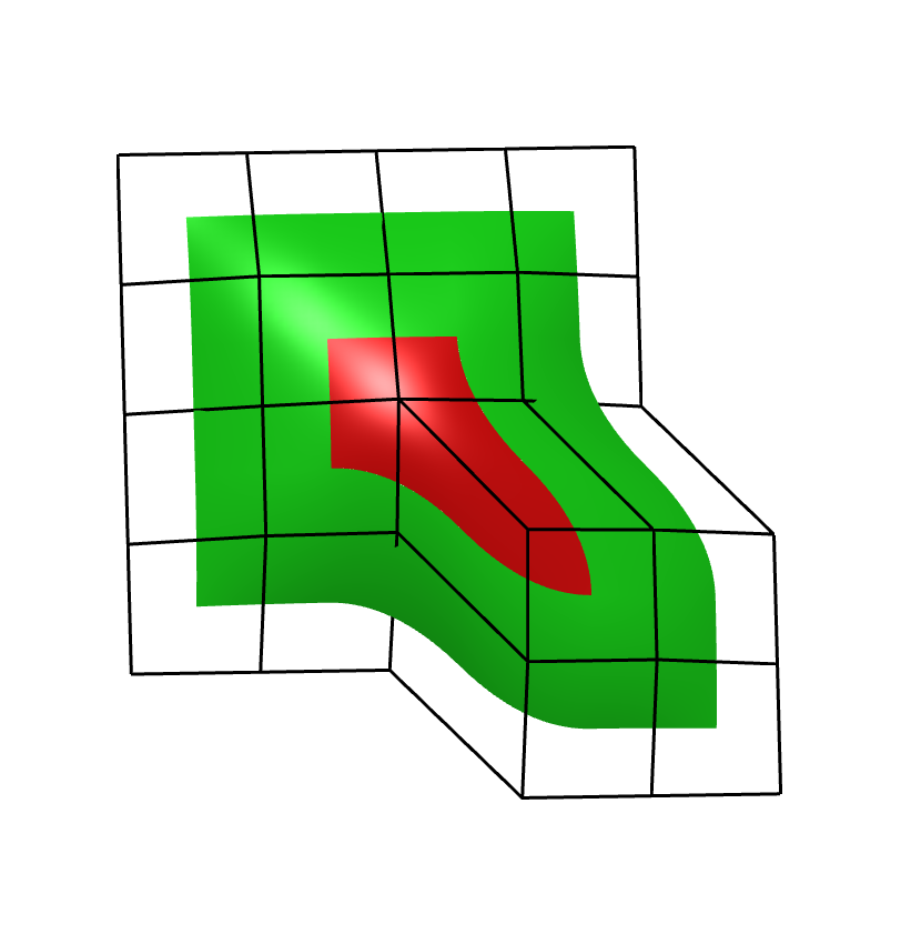
Figure 1: A polyhedral control net and polyhedral spline.

where the tensor-structure breaks down (see the 3-valent and the 5-valent points in Fig. 1) – the B-spline and its control net are not well-defined. Irregularities are no problem for DG spaces. But when the underlying geometry needs to be both curved and smooth, the DG approach comes up short, and requires extra constraints or penalty functions to guarantee a differentiable shape and function space. Such penalty methods require careful calibration to converge to the proper solution. Moreover, depending on the differential equation, a lack of differentiability provides too large a computational space and may so yield outcomes that are not solutions to the original problem, e.g. non-physically discontinuous flow lines. Differentiability across irregularities is therefore both useful and a challenge when devising mathematical software.

Combining differentiability and flexibility, polyhedral splines [38] extend bi-quadratic (bi-2) tensor-product splines on regular, grid-like subnets to the non-tensor product sub-net configurations shown in Fig. 2.

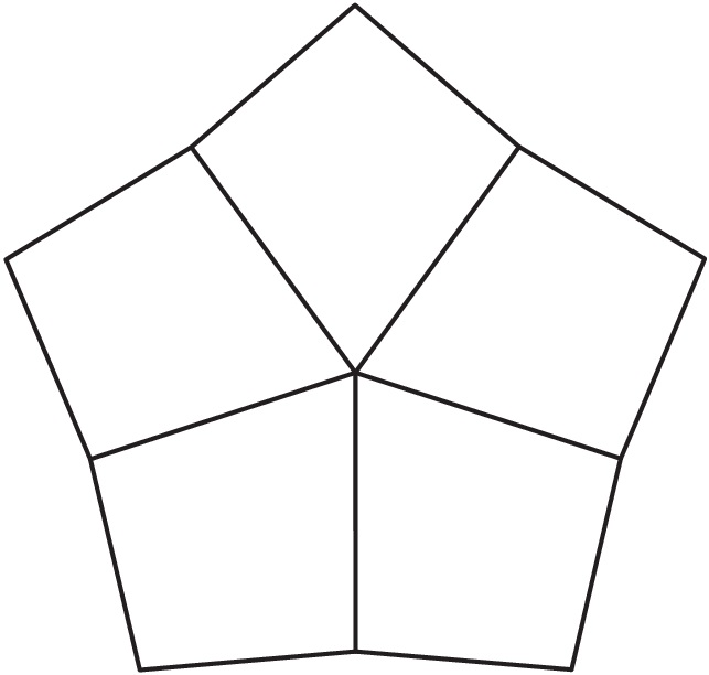
(a) star-net $n=5$

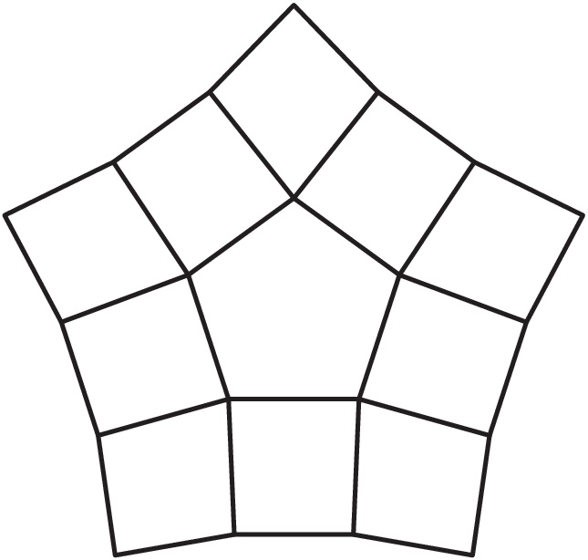
(b) $n$-gon-net, $n=5$

\begin{overpic}[scale={.18},tics=10,width=433.62pt]{fig/polar5.png} \put(10.0,90.0){circular} \put(55.0,55.0){radial} \end{overpic}

(c) polar-net $m=5$

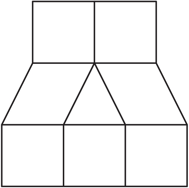
(d) $T_{0}$-net

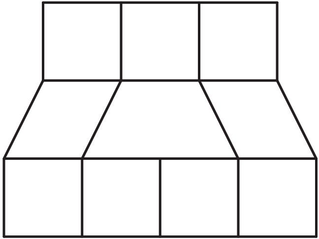
(e) $T_{1}$-net

\begin{overpic}[scale={.18},tics=10,width=433.62pt]{fig/T2.png} \end{overpic}

(f) $T_{2}$-net

Figure 2: Six non-tensor-product polyhedral control net  patterns. The open source code library [38] covers $n,m\in\{3,5,6,7,8\}$.

\begin{overpic}[scale={.18},tics=10,width=433.62pt]{fig/fig19a.jpg} \put(15.0,90.0){polar} \put(40.0,70.0){{\color[rgb]{0,0,0}${n=5}$}} \put(50.0,40.0){{\color[rgb]{1,1,1}$T_{1}$}} \put(65.0,80.0){${n=3}$} \put(80.0,40.0){{\color[rgb]{0,0,0}${n=5}$}} \end{overpic}

(a) polyhedral control net 

\begin{overpic}[scale={.18},tics=10,width=433.62pt]{fig/fig19c.jpg} \put(15.0,90.0){polar} \put(40.0,70.0){{\color[rgb]{0,0,0}${n=5}$}} \put(50.0,40.0){{\color[rgb]{1,1,1}$T_{1}$}} \put(65.0,80.0){${n=3}$} \put(80.0,40.0){{\color[rgb]{0,0,0}${n=5}$}} \end{overpic}

(b) spline patch layout

Figure 3: ‘Bottle opener’ example of a polyhedral spline  combining non-tensor product patterns in close proximity. (a) polyhedral control net with a tight layout: the top pole node is a direct neighbor of four nodes of valence $n=5$. 5-valent nodes are direct neighbors (b) Surface layout including regular bi-quadratic bi-2 splines, $n$-sided star-configurations (blue or gray), bi-3 polar caps, and surface pieces covering $T_{1}$-junctions. See also Fig. 9.

Just like the tensor-product control net, the polyhedral control net expresses the neighbor relations of the polyhedral spline generating functions, outlines shape and provides handles for manipulating the shape: the polyhedral control net vertices can be used as computational degrees of freedom, for least squares fitting, computing moments or for solving partial differential equations. The irregular polyhedral patterns listed in Fig. 2 can be in close proximity, enabling complex layouts such as Fig. 3. A polyhedral spline joins its bi-cubic (bi-3) pieces as a smooth piecewise polynomial function or surface expressed in Bernstein-Bézier form [13]. To introduce creases or discontinuities one can insert facets of zero area, e.g. placing opposing sides of a quad onto each other, or manipulate individual polynomial coefficients of the output. Due to the sharp degree bound proven in [29], there exists no nested polyhedral control net-based refinement (subdivision algorithm) for bi-3 polyhedral splines, but the splines can be refined by de Casteljau’s algorithm [17] applied per piece, or, non-nestedly, by control net subdivision [7].

Overview. After brief overview of alternative smooth polynomial function spaces, Section 2 reviews tensor-product splines, polyhedral control nets and polyhedral splines. Section 3 extends the implementation of polyhedral splines [38] to solve basic partial differential equations on non-tensor-product meshes – without additional meshing.

1.1 Alternative geometric functions spaces

Commonly used computational polynomial spaces for unstructured layout on planar domains include splines on triangulations [30] and radial basis functions [6]. For modeling complex geometric free-form shapes, tensor-product spline (NURBS) domains are carved up into complex regions by a restriction of the domain known as trimming (see e.g. [31] in the context of isogeometric design). Trimming leads to a plethora of downstream challenges due to heterogeneity in size, parameter orientation, continuity and polynomial degree: algebraic, non-rational pre-image curves can result in gaps in the geometry and the complex domains require special integration rules for engineering analysis. The animation industry has instead adopted subdivision surfaces [16] that consist in theory of an infinite sequence of nested surface rings, in practice approximated by a fine faceted model. The survey of splines for irregularities on irregular meshes [37] characterizes subdivision surfaces as one of three singular surface constructions: singularities at corners [35, 41, 34, 48], singular edges [32, 46] and contracting faces, a.k.a. subdivision algorithms [39]. Splines leveraging geometric continuity, i.e. differentiable after a local change of variables include [36, 33, 10, 4] and for data fitting and simulation on planar domains [3, 20, 22, 21]. Analogous to the bi-2 generalizing polyhedral splines in this paper, extending bi-3 tensor-product splines to polyhedral control nets and surfaces of good shape is possible using piecewise polynomials of degree bi-4 or higher, see e.g. [23, 26].

2 Tensor-product splines, polyhedral control nets and polyhedral splines

This section defines and summarizes the evolution of splines on regular tensor-product grids, Section 2.1, to the polyhedral control nets, Section 2.2, of polyhedral splines, Section 2.3.

2.1 Tensor-Product Splines

A tensor-product spline in two variables, $(u,v)$ is a piecewise polynomial function of the form [11] :

$$\mathbf{p}:(u,v)\to\mathbf{p}(u,v):=\sum^{k_{1}}_{i=0}\sum^{k_{2}}_{j=0}\mathbf{c}_{ij}\psi^{d_{1}}_{i}(u)\psi^{d_{2}}_{j}(v).$$ (1)

The coefficients $\mathbf{c}_{ij}$ scale the B-splines $\psi^{d_{\ell}}_{i}$ of degree $d_{\ell}$ and act as degrees of freedom, say for finite element computations or to outline shape. Connecting the control points $\mathbf{c}_{ij}$ to $\mathbf{c}_{i+1,j}$ and $\mathbf{c}_{i,j+1}$ wherever possible yields the control-net. Due to variation diminishing property and the convex hull property, the control-net outlines the graph of the spline function, respectively the geometric shape of the spline surface. Designers edit the control net to shape a surface while automatically maintaining the desired smoothness.

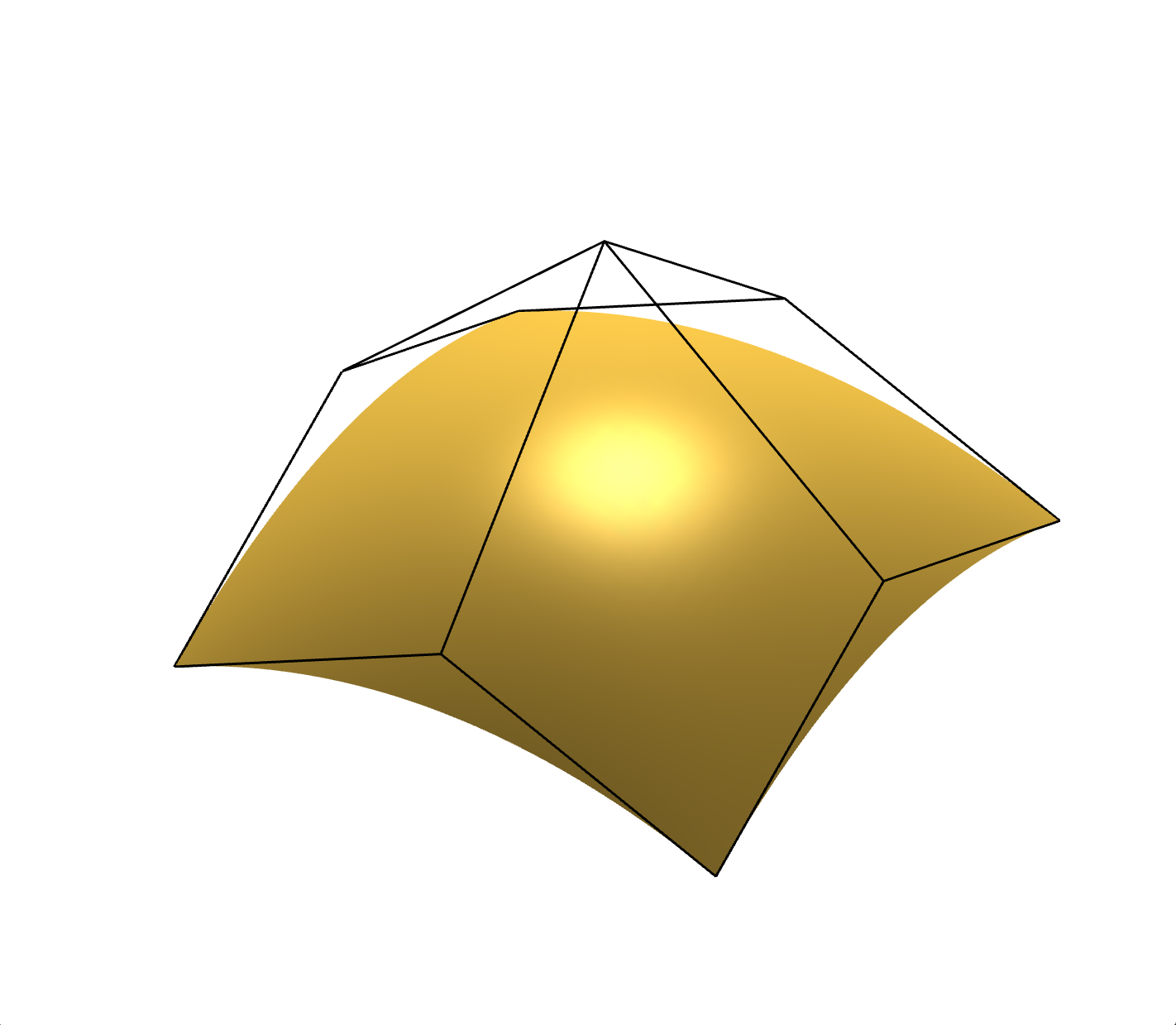
(a) BB-net and bi-2 patch

\begin{overpic}[scale={.18},tics=10,width=433.62pt]{fig/b2bb_bi2.jpg} \put(116.0,46.0){{\color[rgb]{0,1,0}$\Rightarrow$}} \end{overpic}

(b) bi-2 spline nets

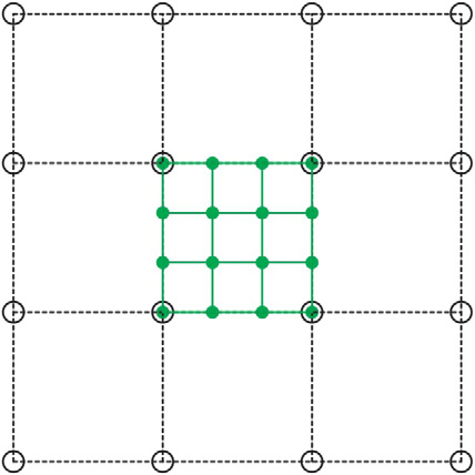
(c) bi-3 spline nets

Figure 4: B-spline control points $\circ$ [11] form a control net and BB-coefficients $\bullet$ [13] form a BB-net of $(d+1)^{2}$ nodes for a polynomial piece of degree bi-$d$. $\Rightarrow$ indicates degree-raising for the BB-form.

Tensor-product spline control nets form grids of $k_{1}\times k_{2}$ quadrilateral faces. Specifically for our setup, any three by three sub-net can be interpreted as the control net of the tensor-product of B-splines $\psi^{2}(t-k)$ of degree 2 with a uniform knot sequence [13] that define one bi-quadratic (bi-2) polynomial piece:

$$\mathbf{p}:(u,v)\to\mathbf{p}(u,v):=\sum^{2}_{i=0}\sum^{2}_{j=0}\mathbf{c}_{ij}\psi^{2}(u-i)\psi^{2}(v-j).$$ (2)

2.2 Patterns in polyhedral control nets

Fig. 2 lists irregular sub-nets of a polyhedral control net and Table 1 succinctly summarizes the structure of the polyhedral layout configurations and the resulting polyhedral splines. Note that for almost all meshes a single Catmull-Clark [7] step guarantees a quad mesh with star configurations only, i.e. a net that controls a polyhedral spline surface.

Meshes consisting of quadrilaterals are popular in polyhedral 3D modeling where quad-strips follow the principal directions and delineate features. Merging $n$ directions forms either a star-net surrounding an extraordinary point of valence $n$, see Fig. 2a, or an $n$-gon, see Fig. 2b. Note that overlapping star configurations are admissible and that a quadrilateral face may have multiple non-4-valent vertices. Fig. 3 demonstrates that irregularities can be placed in close proximity. Often valences $3$ and $5$ suffice for modeling since vertices or faces with valencies $6$, $7$, $8$ can be split and the effect distributed by local re-meshing. However, it is convenient to also have the freedom to include $n=6,7,8$ to avoid re-meshing where multiple surface regions meet. A polar configuration consists of triangles joining at the pole node of high valence to cap off cylindrical structure when modeling finger tips and airplane nose cones. The triangles are interpreted as quadrilaterals with one edge collapsed hence modeled by smoothly joining spline pieces with a (removable) singularity at the pole.

Where two finer quadrilaterals meet a coarser quadrilateral face a T-joint results. This T gives the name to the $T_{1}$-gon (formally a pentagonal face). A $T_{2}$-gon (formally a hexagon) combines two quad-strips at two T-junctions. The $T_{0}$-gon similarly merges neighboring quad-strips without an explicit T-junction.

2.3 Piecewise polynomial polyhedral splines

Table 1: Configurations of polyhedral control nets and polyhedral splines. All patches are in BB-form of degree bi-3. A restriction to $n\in\{3,5,\ldots,8\}$ is only in the distributed code [38]; the underlying theory allows for higher $n$.

configuration
name	center	surrounded by	Fig.	# patches	ref
tensor	$4$-valent point	4 quads	4b	1	[13]
star	$n$-valent	$n$	2(a)	$n$ for $3,5$	[25]
				$4n$ for $n>5$
$n$-gon	$n$-gon	$2n$	2(b)	$n$ for $3,5$	[25]
				$4n$ for $n>5$
$T_{0}$	triangle†	$7$	2(d)	$2\times 2$	[27]
$T_{1}$	pentagon††	$9$	2(e)	$4\times 2$	[27]
$T_{2}$	hexagon†††	$9$	2(f)	$4\times 4$	[27]
polar	$n$-valent	$n$ triangles	2(c)	$n$ degenerate	[28]
† two vertices of valence 4 and one of valence 5. †† four vertices of valence 4 and one of valence 3
††† three consecutive vertices of valence 4 and two of valence 3 separated by one vertex of valence 4

A polyhedral spline  is a collection of smoothly-joined polynomial pieces in Bernstein-Bézier form (BB-form, [13, 17])

$$\mathbf{x}_{(}u,v):=\sum^{d_{1}}_{i=0}\sum^{d_{2}}_{j=0}\mathbf{b}_{ij}b^{d_{1}}_{i}(u)b^{d_{2}}_{j}(v),\ \ \ (u,v)\in[0..1]^{2}$$ (3)

where $b^{d}_{k}(t):=\binom{d}{k}(1-t)^{d-k}t^{k}\in\mathbb{R}$ are the Bernstein polynomials of degree $d$ and $\mathbf{b}_{ij}$ are the BB-coefficients. For surfaces in 3-space, $\mathbf{b}_{ij}\in\mathbb{R}^{3}$ and $\mathbf{x}$ is a piece of the surface, called a patch. For example, a bi-3 patch has $4\times 4$ BB-coefficients as in Fig. 4c. Connecting $\mathbf{b}_{ij}$ to $\mathbf{b}_{i+1,j}$ and $\mathbf{b}_{i,j+1}$ wherever possible yields the BB-net. The BB-net is usually finer than the B-spline control net of the same polynomial pieces. (The BB-net represents a single polynomial piece whereas the B-spline control net represents a piecewise polynomial function. However, Any B-spline can be expressed as multiple pieces of polynomials in BB-form and any basis function of the BB-form can be expressed in B-spline form with suitably repeated knots [12, 13].) The BB-form is evaluated via de Casteljau’s algorithm [47], differentiated exactly by forming differences of the BB-coefficients and exactly integrated by forming sums [17]. To obtain a uniform degree bi-3 in all cases, any patch of degree lower than bi-3 can be expressed as a patch of degree bi-3 by a process called degree-raising [13, 17]. Degree bi-3 is therefore the default for the polyhedral splines used in this paper.

\begin{overpic}[scale={.18},tics=10,width=433.62pt]{fig/geomCont.png} \put(40.0,27.0){$\mathbf{x}$} \put(40.0,9.0){$\mathbf{q}$} \put(0.0,10.0){$\beta$} \put(5.0,-3.0){$u$} \put(22.0,19.0){$u$} \put(65.0,15.0){$E$} \end{overpic}

Figure 5: Geometric smoothness between patches $\mathbf{x}$ and $\mathbf{q}$ to form an atlas.

The polyhedral spline pieces join by default without gaps or overlap and with matching first derivatives – possibly after a reparameterization (a change of variables) as is appropriate for manifolds. Focusing on the shared boundary $E$ between two abutting patches $\mathbf{p}$ and $\mathbf{q}$, see Fig. 5. Let $\beta:\mathbb{R}^{2}\to\mathbb{R}$, $\beta(u):=(u+b(u)v,a(u)v)$ be a (local) reparameterization and $\mathbf{p}(u,0)=E=\mathbf{q}(u,0)$. We say that $\mathbf{q}$ and $\mathbf{p}$ join $G^{1}$ if the partial derivatives lie in the same plane and the transversal $v$-derivatives of the two patches lie on opposite sides with respect to the $u$-derivative along the shared boundary:

$$\partial_{v}\mathbf{q}(u,0)+a(u)\partial_{v}\mathbf{p}(u,0)=b(u)\partial_{u}\mathbf{p}(u,0),\quad a(u)\neq 0,\ u\in[0..1].$$ (4)

When $b(u):=0$ and $a(u):=const$, then we say the spline pieces join parameterically $C^{1}$. Tensor-product and polar polyhedral splines are internally $C^{1}$ (polar splines with a removable singularity at the pole, see [28]). Otherwise the spline pieces join with geometric smoothness, short $G^{1}$. For example, [25] uses a quadratic change of variables to transition from the surrounding surface to one of the $n$ bi-3 patches of the cap and a linear one between adjacent bi-3 patches of the cap. The result are explicit formulas that relate the input polyhedral net to the output BB-coefficients of the polyhedral spline, see [25], [27], [28]. We note that at global boundaries, as is typical for not-a-knot splines, the outermost layer recedes as in Fig. 1.

3 Computing with polyhedral splines

Bi-cubic polyhedral splines have many applications including industrial design, visualization, animation, moment computation, re-approximation, reconstruction, computation of partial differential equations on manifolds, etc.. For example, [33] uses a sub-class of polyhedral spline functions, for star-configurations only, to solve fourth order partial differential equations, and to compute geodesics on a free-form polyhedral spline surface via the heat equation.

The appeal of polyhedral spline is that the applications are supported by the same representation as the geometry, without additional meshing. The irregular patterns can be viewed as both structurally necessary but also as a form of local adaptation.

First, in Section 3.1, 3.2 and 3.3, we test the new elements by artificially introducing irregular polyhedral patterns into an otherwise regular grid to be able to compare with a known exact solution. The experiments indicate that the irregular patterns in polyhedral splines do not noticeably increase the local error. Second, in Section 3.4, we compute second-order equations on a free-form surface modeled by polyhedral splines.

3.1 Poisson Test

We evaluate the impact of inserting irregular mesh patterns on the error by solving a standard problem, Poisson’s equation over the physical domain $\Omega=\mathbf{x}(\Box)$, where $\Box:=[-1..1]^{2})$:

$$\text{find }\mathtt{u}:\Omega\rightarrow\mathbb{R}:\begin{cases}\Delta\mathtt{u}&=-f\hskip 8.53581pt\text{ in }\Omega,\\ \hphantom{\Delta}\mathtt{u}&=0\hskip 19.91692pt\text{ on }\partial\Omega.\end{cases}$$ (5)

The weak form of Poisson’s equation, projected into the $C^{1}$ space of polyhedral spline basis functions $\phi_{j}$, is by Galerkin’s approach,

$$\int_{\Omega}\nabla\mathtt{u}_{h}\cdot\nabla\phi_{i}(\mathbf{x}^{-1}{})d_{\Omega}=\int_{\Omega}f\phi_{i}(\mathbf{x}^{-1}{})d_{\Omega},\quad\mathtt{u}_{h}:=\sum_{j}\mathbf{c}_{j}\phi_{j}(\mathbf{x}^{-1}{}).$$

The equation can be rewritten as the matrix equation $K\mathbf{c}=\mathbf{f}$ to be solved for the coefficient vector $\mathbf{c}$ of $\mathtt{u}_{h}$ where

$$K_{ij} :=\sum_{\alpha}\int_{\Box}(\nabla\phi_{i})^{\mathtt{t}}(J_{\alpha}^{\mathtt{t}}J_{\alpha})^{-1}(\nabla\phi_{j})\operatorname{d}\Box,\quad J_{\alpha}:=\nabla_{\mathbf{s}}\mathbf{x}_{\alpha},$$ (6)

$$\mathbf{f}_{i} :=\sum_{\alpha}\int_{\Box}f\cdot\ \phi^{i}_{\cdot}\mathtt{J}\ \operatorname{d}\Box,\quad\mathtt{J}:=\sqrt{\operatorname{det}(J_{\alpha}^{\mathtt{t}}J_{\alpha})}.$$ (7)

Here the sum is over all pieces $\alpha$ where $\phi_{i}$ has support.

(a) Input: cube.obj

\begin{overpic}[unit=1mm,scale={.25},width=433.62pt]{fig/cube_hl.png} \put(-40.0,30.0){$\Longrightarrow$} \end{overpic}

(b) surface

Figure 6: [38] The input .obj file and the output polyhedral spline surface visualized with highlight lines in Bézierview [40].

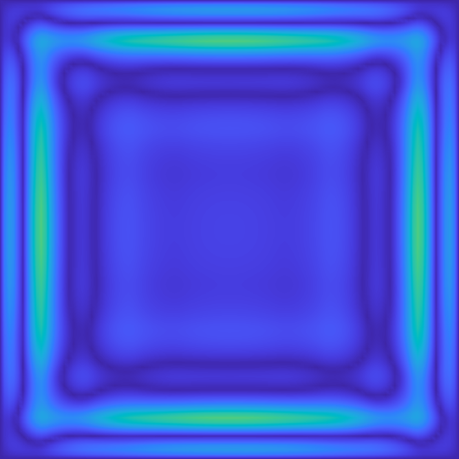
(a) regular grid

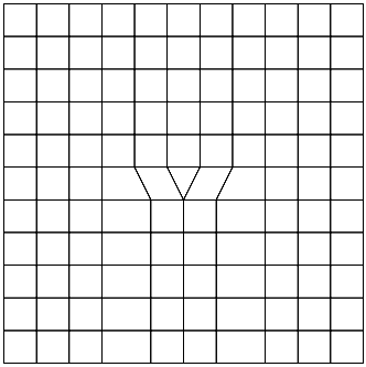
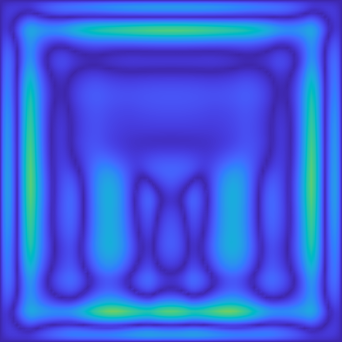
(b) T0

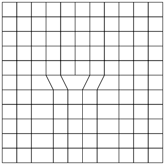
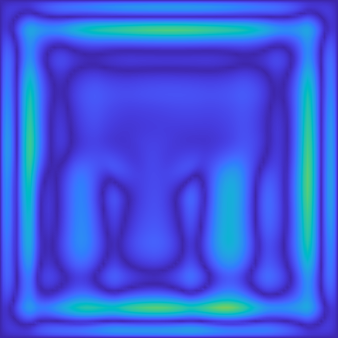
(c) T1 subtract

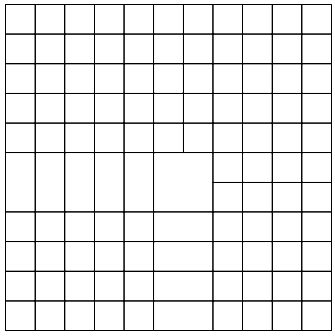
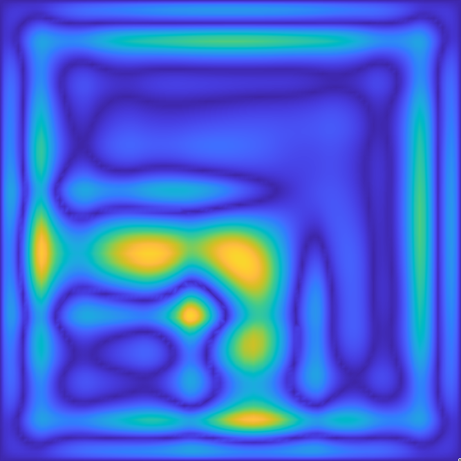
(d) T2 subtract

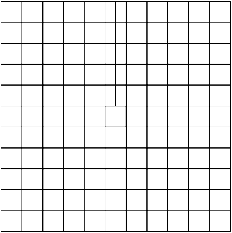
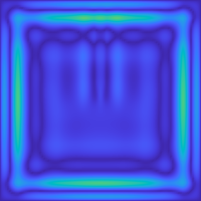
(e) T1 add

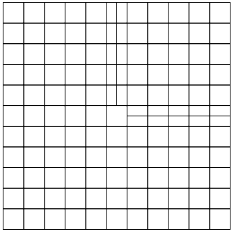
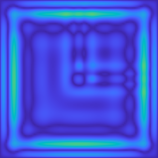
(f) T2 add

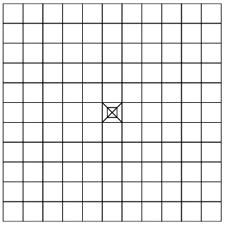
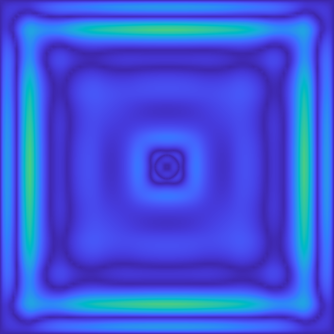
(g) polar-net $n=4$

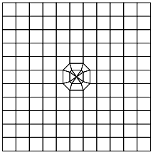
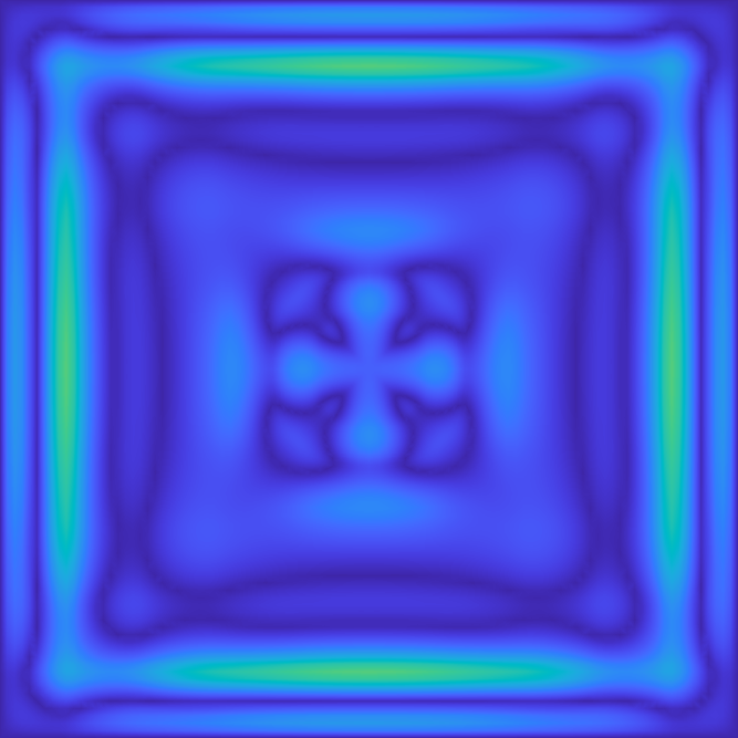
(h) polar-net $n=8$

\begin{overpic}[scale={.18},tics=10,width=433.62pt]{fig/Colorbar-no-labels.png} \put(0.0,-4.0){0} \put(29.0,-4.0){0.005} \put(63.5,-4.0){0.01} \put(91.5,-4.0){0.015} \end{overpic}

Figure 7: Absolute error between approximate solution and exact solution for the various polyhedral control net configurations. The exact solution $\mathtt{u}=(u^{2}-1)(v^{2}-1)$ varies between $0$ and $1$ on the domain $[-1..1]^{2}$.

3.2 Implementation Details

The code [38] collects the seven sub-net configurations from the input faceted free-form topological polyhedron (in .obj format [45], see Fig. 6a) and generates the BB-coefficients of the pieces of a smooth spline that can be visualized by the online webGL viewer at [40], see Fig. 6b. Each $x$, $y$, $z$ coordinate is a polyhedral spline. We intercept the output to compute the geometry terms $(J_{\alpha}^{\mathtt{t}}J_{\alpha})^{-1}$ and $\mathtt{J}$ and access the connectivity information to determine where basis functions $\phi_{i}$ overlap in support to minimize the computational work in assembling $K$ and $\mathbf{f}$. Exact derivative polynomials are obtained by differencing BB-coefficients, e.g. $\mathbf{b}_{{i+1},j}-\mathbf{b}_{i,j}$ for differentiation with respect to the first variable. For integration, all functions are evaluated at Gauss points, shifted to the interval $[0..1]$ that is natural for the BB-form. Assembly is therefore no more costly than for tensor-product splines.

We enforce the boundary constraints by modifying the basis functions overlapping the boundary, setting to zero the BB-coefficients that determine $\phi_{j}$ on the boundary and beyond (Recall that the surface boundary recedes by a half from the boundary of the control polygon, Fig. 1.) Here we interpret the outermost control points as belonging to bi-quadratic splines: they do, but have been degree-raised. Since for a bi-quadratic spline the only non-zero coefficient within the domain is on the boundary, we can ignore their contribution. We note that this approach may fail at corners for the $H^{1}$ norm since setting two partial derivatives to zero forces the derivatives at the corner to be zero.

3.3 Error for Poisson’s equation

To accurately measure the error, and so gauge the impact of the irregular polyhedral control net configurations, we choose a trivial geometric (physical surface) domain $x(u,v)=u$, $y(u,v)=v$, $z(u,v)=0$ to cover $[-1..1]^{2}$. That is, we compute the graph of a function in the knowledge that computations on more complex free-form surfaces are no more difficult in the implemented framework (see Fig. 9), only harder to verify due to the lack of explicit solutions for free-form surfaces. We choose $f:=2(u^{2}+v^{2}-2)$ so that we know the exact solution of (5) to be $\mathtt{u}=(u^{2}-1)(v^{2}-1)$.

Starting with the tensor grid on $[-1..1]^{2}$ as a basic test, we solve and display the absolute difference between the polyhedral splines and the exact solution of (5) in Fig. 7. Although the exact solution is bi-quadratic, enforcing the boundary constraints with fixed resolution results in an error along and near the boundary, of less than 1% see Fig. 7(a). Note the error bar Fig. 7. Fig. 7(c) and Fig. 7(d) are obtained by removing grid-lines from Fig. 7(a) whereas Fig. 7(e) and Fig. 7(f) are obtained by adding grid-lines. The location and disappearance of the subtractive case maximal errors shows that the error is dominated by the reduction in the degrees of freedom when eliminating half a column and half a row of control points, and not due to distortion near the T-configuration. Fig. 7(c), 7(d), 7(e) and 7(f) remind of T-splines. However, T-splines [43, 19] start with quadrilaterals and require a global parameterization and then insert partitions and T-junctions. In general, the input free-form control nets cannot already include T-junctions [24, Fig 18]. Fig. 7(g) and Fig. 7(h) add minimal polar configurations with a decrease in error near the pole and no noteworthy increase in error in the neighborhood.

We do not show convergence rates under refinement because the polyhedral spline patterns do not have a natural refinement and since the 2-norm error under refinement, by splitting quadrilaterals into $2\times 2$ or by applying Catmull-Clark subdivision to the polyhedral control net, is anyhow dominated by the regular mesh and the resulting spaces are not nested due to the different extent of the geometric continuity. To obtain nested refinement, each quadrilateral bi-3 patch in BB-form can internally be partitioned and replaced by a $C^{1}$-connected spline complex that provides a local refinement hierarchy, the well-known T-spline space of ‘elements with hanging nodes’, see e.g.  [19].

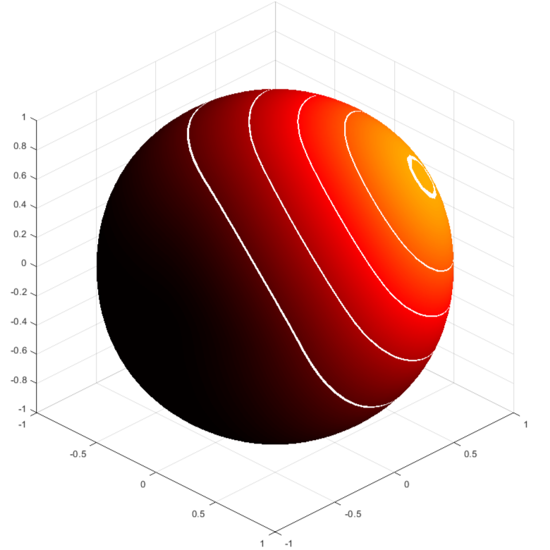
(a) $t=0$

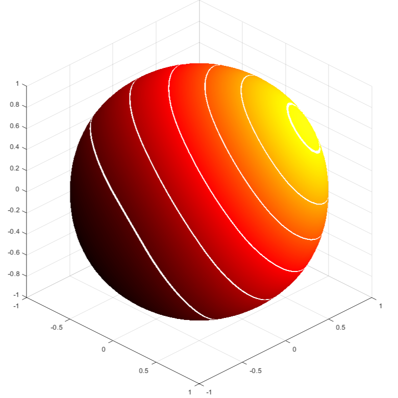
(b) $t=0.25$

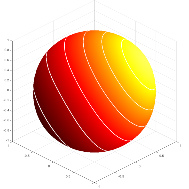
(c) $t=0.5$

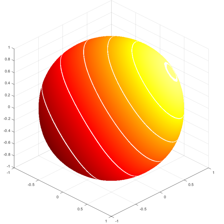
(d) $t=0.75$

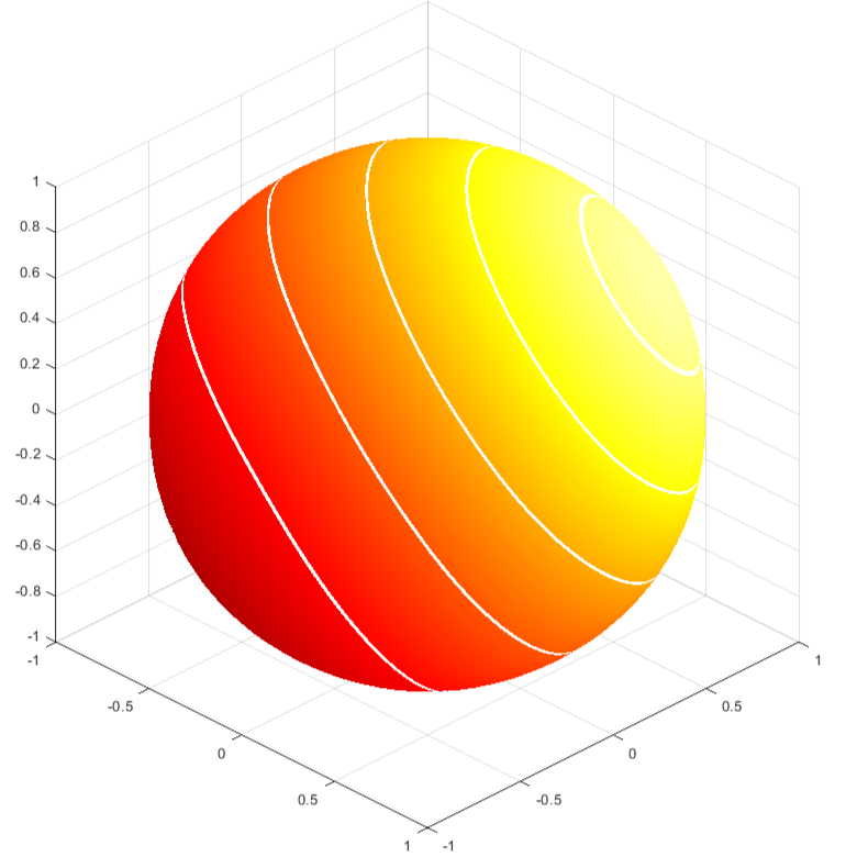
(e) $t=1$

\begin{overpic}[scale={.18},tics=10,width=433.62pt]{fig/colorbar_cube} \put(0.0,-4.0){0} \put(10.5,-4.0){10} \put(23.0,-4.0){20} \put(35.5,-4.0){30} \put(48.0,-4.0){40} \put(60.5,-4.0){50} \put(73.0,-4.0){60} \put(85.5,-4.0){70} \put(96.0,-4.0){80} \end{overpic}

Figure 8: Progression of geodesic fronts over time $t$ when solving the heat equation over the polyhedral spline with input specified in Fig. 6. The temperature at the upper right vertex, the heat source, is kept constant to $80^{\circ}$.

3.4 Computing on free-form surfaces

Having verified correctness of the implementation on the a square domain for all configurations, we solve the heat equation on polyhedral spline free-form surfaces, i.e. a second-order elliptic partial differential equation with a solution evolving over time. To certify correctness of the implementation, we start with the simple cube (8 nodes, 6 faces) of Fig. 6. We seed the temperature at one of the 8 vertices of the cube and observe the progress of the heat level curves over time. This yields a progression of geodesic fronts, as illustrated by the white lines in Fig. 8.

(a) $t=0.5$

(b) $t=0.75$

(c) $t=1$

\begin{overpic}[scale={.18},tics=10,width=433.62pt]{fig/colorbar_cube} \put(0.0,-4.0){0} \put(10.5,-4.0){10} \put(23.0,-4.0){20} \put(35.5,-4.0){30} \put(48.0,-4.0){40} \put(60.5,-4.0){50} \put(73.0,-4.0){60} \put(85.5,-4.0){70} \put(96.0,-4.0){80} \end{overpic}

Figure 9: Progression of geodesic fronts for the polyhedral spline  with ‘bottle opener’ input specified in Fig. 3 exposed to Florida sun at the upper left corner. (a) A low gradient causes a wide white level indicator curve at the lower right. The surface has no gaps.

Finally, to test a complex and tight ensemble of polyhedral configurations, we compute the heat progression on the‘bottle opener’ of Fig. 3. Fig. 9 shows the time series before the opener becomes too hot to handle.

4 Conclusion

Analogous to tensor-product splines, but for more general control net configurations, polyhedral splines have been shown to model curved geometry (without trimming) and to represent higher-order functions on that geometry. This setup has potential to be used for engineering analysis on curved smooth objects without additional meshing. As a proof-of-concept, we derived time-evolving solutions of an elliptic partial differential equation. Since polyhedral splines are differentiable, also fourth-order equation Galerkin solvers make sense and can be implemented.

Acknowledgement We thank William Gregory for support with C++ programming and Kyle Lo for generating input models and explaining data structures of the polyhedral spline code.

References

- [1]
- Au and Cheung [1993] F.T.K. Au and Y.K. Cheung. 1993. Isoparametric Spline Finite Strip for Plane Structures. Computers & Structures 48 (1993), 22–32.
- Bercovier and Matskewich [2017] Michel Bercovier and Tanya Matskewich. 2017. Smooth Bézier Surfaces over Unstructured Quadrilateral Meshes. Lecture Notes of the Unione Matematica Italiana (2017).
- Blidia et al. [2020] Ahmed Blidia, Bernard Mourrain, and Gang Xu. 2020. Geometrically smooth spline bases for data fitting and simulation. Computer Aided Geometric Design 78 (March 2020), 101814.
- Braibant and Fleury [1984] V. Braibant and C. Fleury. 1984. Shape Optimal Design using B-splines. Computer Methods in Applied Mechanics and Engineering 44 (1984), 247–267.
- Buhmann [2009] Martin D. Buhmann. 2009. Radial Basis Functions - Theory and Implementations. Cambridge monographs on applied and computational mathematics, Vol. 12. Cambridge University Press. I–X, 1–259 pages. http://www.cambridge.org/de/academic/subjects/mathematics/numerical-analysis/radial-basis-functions-theory-and-implementations
- Catmull and Clark [1978] E. Catmull and J. Clark. 1978. Recursively generated B-spline surfaces on arbitrary topological meshes. Computer-Aided Design 10 (Sept. 1978), 350–355.
- Cirak et al. [2000] F. Cirak, M. Ortiz, and P. Schröder. 2000. Subdivision surfaces: a new paradigm for thin-shell finite-element analysis. Internat. J. Numer. Methods Engrg. 47 (April 2000).
- Cockburn et al. [2000] B. (Bernardo) Cockburn, George Karniadakis, and Chi-Wang Shu. 2000. Discontinuous Galerkin methods: theory, computation, and applications. Vol. 11. Springer-Verlag Inc., pub-SV:adr. xi + 470 pages.
- Collin et al. [2016] Annabelle Collin, Giancarlo Sangalli, and Thomas Takacs. 2016. Analysis-suitable G1 multi-patch parametrizations for C1 isogeometric spaces. Computer Aided Geometric Design 47 (2016), 93–113.
- de Boor [1978] C. de Boor. 1978. A Practical Guide to Splines. Springer.
- de Boor [1986] Carl de Boor. 1986. B (asic)-Spline Basics. Technical Report. U of Wisconsin, Mathematics Research Center.
- de Boor [1987] C. de Boor. 1987. B-form basics. In Geometric Modeling: Algorithms and New Trends, G. Farin (Ed.). SIAM, 131–148.
- Demkowicz and Gopalakrishnan [2010] Leszek Demkowicz and Jayadeep Gopalakrishnan. 2010. A class of discontinuous Petrov–Galerkin methods. Part I: The transport equation. Computer Methods in Applied Mechanics and Engineering 199, 23-24 (2010), 1558–1572.
- Demkowicz and Gopalakrishnan [2011] Leszek Demkowicz and Jayadeep Gopalakrishnan. 2011. A class of discontinuous Petrov–Galerkin methods. II. Optimal test functions. Numerical Methods for Partial Differential Equations 27, 1 (2011), 70–105.
- DeRose et al. [1998] Tony DeRose, Michael Kass, and Tien Truong. 1998. Subdivision Surfaces in Character Animation. ACM Press, New York, 85–94.
- Farin [1988] Gerald Farin. 1988. Curves and Surfaces for Computer Aided Geometric Design: A Practical Guide. Academic Press.
- Hughes et al. [2005] T. J. R. Hughes, J. A. Cottrell, and Y. Bazilevs. 2005. Isogeometric Analysis: CAD, Finite Elements, NURBS, Exact Geometry and Mesh Refinement. Computer Methods in Applied Mechanics and Engineering 194 (2005), 4135–4195.
- Kang et al. [2015] Hongmei Kang, Jinlan Xu, Falai Chen, and Jiansong Deng. 2015. A new basis for PHT-splines. Graphical Models 82 (2015), 149–159.
- Kapl et al. [2018] Mario Kapl, Giancarlo Sangalli, and Thomas Takacs. 2018. Construction of analysis-suitable G1 planar multi-patch parameterizations. Computer-Aided Design 97 (2018), 41–55.
- Kapl et al. [2019a] Mario Kapl, Giancarlo Sangalli, and Thomas Takacs. 2019a. Isogeometric analysis with functions on planar, unstructured quadrilateral meshes. The SMAI journal of computational mathematics (2019), 67–86.
- Kapl et al. [2019b] Mario Kapl, Giancarlo Sangalli, and Thomas Takacs. 2019b. An isogeometric C 1 subspace on unstructured multi-patch planar domains. Computer Aided Geometric Design 69 (2019), 55–75.
- Karčiauskas et al. [2016] Kȩstutis Karčiauskas, Thien Nguyen, and Jörg Peters. 2016. Generalizing bicubic splines for modeling and IGA with irregular layout. Computer-Aided Design 70 (2016), 23–35.
- Karčiauskas et al. [2017] Kȩstutis Karčiauskas, Daniele Panozzo, and Jörg Peters. 2017. T-junctions in spline surfaces. ACM Transactions on Graphics (TOG) 36, 5 (2017), 1–9.
- Karčiauskas and Peters [2015] Kȩstutis Karčiauskas and Jörg Peters. 2015. Smooth multi-sided blending of biquadratic splines. Computers & Graphics 46 (2015), 172–185.
- Karčiauskas and Peters [2019] Kȩstutis Karčiauskas and Jörg Peters. 2019. High quality refinable G-splines for locally quad-dominant meshes with T-gons. In Computer Graphics Forum, Vol. 38. Wiley Online Library, 151–161.
- Karčiauskas and Peters [2020a] Kȩstutis Karčiauskas and Jörg Peters. 2020a. Low degree splines for locally quad-dominant meshes. Computer Aided Geometric Design 83 (2020), 1–12.
- Karčiauskas and Peters [2020b] Kȩstutis Karčiauskas and Jörg Peters. 2020b. Smooth polar caps for locally quad-dominant meshes. Computer Aided Geometric Design 81 (06 2020), 1–12. https://doi.org/10.1016/j.cagd.2020.101908 PMC7343232.
- Karčiauskas and Peters [2021] Kȩstutis Karčiauskas and Jörg Peters. 2021. Least Degree -refinable Multi-sided Surfaces Suitable for Inclusion into bi-2 Splines. Computer-Aided Design 130 (2021), 1–12.
- Lai and Schumaker [2007] Ming-Jun Lai and Larry L. Schumaker. 2007. Spline Functions on Triangulations. Cambridge University Press. https://doi.org/10.1017/CBO9780511721588
- Marussig and Hughes [[n. d.]] B Marussig and TJR Hughes. [n. d.]. A Review of Trimming in Isogeometric Analysis: Challenges, Data Exchange and Simulation Aspects. Arch Comput Methods Eng. 25, 4 ([n. d.]), 1059–1127. Erratum in: Arch Comput Methods Eng. 2018;25(4):1131..
- Myles and Peters [2011] Ashish Myles and Jörg Peters. 2011. C2 splines covering polar configurations. Computer-Aided Design 43, 11 (2011).
- Nguyen et al. [2016] Thien Nguyen, Kȩstutis Karčiauskas, and Jörg Peters. 2016. finite elements on non-tensor-product 2d and 3d manifolds. Appl. Math. Comput. 272, 1 (2016), 148–158.
- Nguyen and Peters [2016] Thien Nguyen and Jörg Peters. 2016. Refinable spline elements for irregular quad layout. Computer Aided Geometric Design 43 (March 29 2016), 123–130.
- Peters [1991] J. Peters. 1991. Smooth interpolation of a mesh of curves. Constructive Approximation 7 (1991), 221–247.
- Peters [1995] J. Peters. 1995. -surface splines. SIAM J. Numer. Anal. 32, 2 (1995), 645–666.
- Peters [2019] J. Peters. 2019. Splines for Meshes with Irregularities. The SMAI journal of computational mathematics S5 (2019), 161–183.
- Peters et al. [2023] Jörg Peters, Kyle Lo, and Kȩstutis Karčiauskas. 2023. Algorithm 1032: Bi-cubic splines for polyhedral control nets. ACM Tr on Math Software 49 (March 2023). Issue 1.
- Peters and Reif [2008] J. Peters and U. Reif. 2008. Subdivision Surfaces. Geometry and Computing, Vol. 3. Springer-Verlag, New York. i–204 pages.
- Peters and Wu [2021] J. Peters and X. Wu. 2021. BezierView (short bview): a light weight viewer that renders Bezier patches. https://www.cise.ufl.edu/research/SurfLab/bview
- Reif [1998] Ulrich Reif. 1998. TURBS—Topologically Unrestricted Rational B-Splines. Constructive Approximation 14 (1998), 57–77.
- Schramm and Pilkey [1993] Uwe Schramm and Walter D. Pilkey. 1993. The coupling of geometric descriptions and finite elements using NURBS - A study in shape optimization. Finite elements in Analysis and Design 340 (1993), 11–34.
- Sederberg et al. [2003] Thomas W Sederberg, Jianmin Zheng, Almaz Bakenov, and Ahmad Nasri. 2003. T-splines and T-NURCCs. ACM transactions on graphics (TOG) 22, 3 (2003), 477–484.
- Shyy et al. [1988] Y.K. Shyy, C. Fleury, and K. Izadpanah. 1988. Shape Optimal Design using higher-order elements. Computer Methods in Applied Mechanics and Engineering 71 (1988), 99–116.
- Technologies [2021] Wavefront Technologies. 2021. Wavefront .obj file. https://en.wikipedia.org/wiki/Wavefront_.obj_file
- Toshniwal et al. [2017] D Toshniwal, H Speleers, R R Hiemstra, and TJR Hughes. 2017. Multi-degree smooth polar splines: A framework for geometric modeling and isogeometric analysis. Computer Methods in Applied Mechanics and Engineering 316 (2017), 1005–1061.
- Wikipedia contributors [2021] Wikipedia contributors. 2021. De Casteljau’s algorithm — Wikipedia, The Free Encyclopedia. https://en.wikipedia.org/w/index.php?title=De_Casteljau%27s_algorithm&oldid=1043959654 [Online; accessed 1-December-2021].
- Wu et al. [2017] Meng Wu, Bernard Mourrain, André Galligo, and Boniface Nkonga. 2017. Hermite Type Spline Spaces over Rectangular Meshes with Complex Topological Structures. Communications in Computational Physics 21, 3 (2017), 835–866.