Abstract

Background: Dose-finding studies often include an up-and-down dose transition rule that assigns a dose to each cohort of patients based on accumulating data on dose-limiting toxicity (DLT) events. In making a dose transition decision, a key scientific question is whether the true DLT rate of the current dose exceeds the target DLT rate, and the statistical question is how to evaluate the statistical evidence in the available DLT data with respect to that scientific question.

Methods: I propose to use generalized likelihood ratios (GLRs) to measure statistical evidence and support dose transition decisions. This leads to a GLR-based interval design with three parameters: the target DLT rate and two GLR cut-points representing the levels of evidence required for dose escalation and de-escalation. The GLR-based design gives a likelihood interpretation to each existing interval design and provides a unified framework for comparing different interval designs in terms of how much evidence is required for escalation and de-escalation.

Results: A GLR-based comparison of four popular interval designs reveals that the BOIN and TEQR designs require similar amounts of evidence for escalation and de-escalation, while the mTPI and i3+3 designs require more evidence for de-escalation than for escalation. Simulation results demonstrate that the last two designs tend to produce higher proportions of over-treated patients than the first two. These observations motivate the consideration of GLR-based designs that require more evidence for escalation than for de-escalation. Such designs are shown to reduce the proportion of over-treated patients while maintaining the same accuracy of dose selection, as compared to the four popular interval designs.

Conclusions: GLRs are useful tools for understanding, comparing and constructing interval designs of dose-finding studies. GLR-based designs that require more evidence for escalation than for de-escalation can help reduce over-treatment without sacrificing dose selection accuracy.

Key words: dose de-escalation; dose escalation; dose selection; dose transition; generalized law of likelihood; isotonic regression; monotonicity; phase 1 trial design

1 Introduction

Clinical research on novel therapeutic agents usually starts with dose-finding studies, which aim to identify one or more promising doses for further evaluation. A major focus in such studies is the frequency of dose-limiting toxicity (DLT) events and the maximum tolerated dose (MTD), defined as the highest dose among those considered that has a DLT rate not exceeding a specified value (i.e., the target DLT rate). The MTD is of particular interest when drug activity is expected to increase with increasing dose and when early measures of activity are unavailable or unreliable.

Popular designs for finding the MTD include the well-known 3+3 design (Storer, 1989; Korn et al., 1994), the continual reassessment method (CRM; O’Quigley et al., 1990), the accelerated titration design (Simon et al., 1997), the modified toxicity probability interval (mTPI) design (Ji et al., 2010), the toxicity equivalence range (TEQR) design (Blanchard and Longmate, 2011), the Bayesian optimal interval design (BOIN) design (Liu and Yuan, 2015), the i3+3 design (Liu et al., 2020), and many others. Most of these designs include an up-and-down dose transition rule that assigns a dose to each cohort of patients based on accumulating DLT data, and an MTD estimation procedure to be applied to all available data at the end of the study. For interval designs (mTPI, TEQR, BOIN and i3+3), the dose transition rule amounts to locating the observed DLT rate at the current dose in one of three intervals corresponding to three possible actions (escalate, de-escalate, or stay).

In making a dose transition decision, a key scientific question to consider is whether the true DLT rate of the current dose exceeds the target DLT rate. If the right answer to this question is known with certainty, the right action to take would be obvious (de-escalate if the answer is yes; escalate if the answer is no), and there would be no need to stay. In reality, the right answer is unavailable, and one has to rely on statistical evidence in the available data to make a decision. One may decide to escalate or de-escalate if the evidence is interpreted as providing adequate support for such an action. If there is not enough evidence to support either action, one may decide to stay at the current dose and collect more data. From this perspective, any dose transition rule can be regarded as a way to interpret statistical evidence in the available DLT data with respect to the key scientific question stated above.

In this article, I propose to use generalized likelihood ratios (GLRs) to interpret and quantify statistical evidence in making dose transition decisions. The GLR is a measure of statistical evidence for comparing two composite hypotheses according to the generalized law of likelihood (GLL; Bickel, 2008; Zhang and Zhang, 2013), which generalizes the law of likelihood for comparing two simple hypotheses (Hacking, 1965; Royall, 1997; Blume, 2002). When applied to the dose transition problem, the GLL leads to a GLR-based interval design comparable to existing interval designs. Different interval designs can often be calibrated to match or mimic each other (e.g., BOIN and TEQR). Likewise, the GLR-based design can be related to the other interval designs by calculating GLRs at decision boundaries for the other designs. Through these connections, the GLR-based design gives a likelihood interpretation to each existing interval design and provides a unified framework for comparing different interval designs in terms of how much evidence they require for escalation and de-escalation. This comparison reveals major differences between different designs with important implications on patient safety, and motivates new configurations of interval designs (based on the GLR) with the potential to improve patient safety.

To compute the GLR, one could use a single-dose likelihood based on the available DLT data at the current dose, or a joint likelihood based on all available DLT data at different doses under an isotonic regression model. For simplicity and comparability with the other interval designs, I will focus on the single-dose likelihood initially before introducing the joint likelihood and comparing their operating characteristics.

There is increasing awareness that dose-finding studies should consider both toxicity and activity, especially for targeted therapies in oncology with a non-monotone dose-activity relationship (Cook et al., 2015; Wages et al., 2018; Shah et al., 2021; FDA, 2023). This awareness has motivated a new class of designs aiming to find the optimal biological dose (OBD), such as extended mTPI and TEQR designs (Li et al., 2016; Ananthakrishnana et al., 2018), extended BOIN designs (Takeda et al., 2018; Lin et al., 2020), extended CRM designs (Wages and Tait, 2015; Aout and Seroutou, 2018), and various adaptive designs (Zang et al., 2014; Chiuzan et al., 2018). The GLL can be applied to accumulating activity data to evaluate statistical evidence about the dose-activity relationship; in fact, that was the original motivation for this research. Designing an OBD-finding study requires careful considerations for both toxicity and activity assessments, each of which deserves considerable attention. This article, with focus on toxicity, can be viewed a first step in developing a GLR-based design for finding the OBD.

2 Methods

2.1 Review of GLL and GLR

Suppose data are observed under a parametric model with parameter $\theta\in\Theta$. Let $L(\theta)$ be the likelihood for $\theta$ based on the observed data, and let $\theta_{1}$ and $\theta_{2}$ be distinct values in $\Theta$. According to the law of likelihood (Hacking, 1965), the observed data provide statistical evidence supporting the hypothesis $\theta=\theta_{1}$ over the hypothesis $\theta=\theta_{2}$ if $L(\theta_{1})>L(\theta_{2})$, and the likelihood ratio (LR), $L(\theta_{1})/L(\theta_{2})$, measures the strength of that evidence. From a Bayesian perspective, the LR can be interpreted as an invariant Bayes factor for an arbitrary prior distribution of $\theta$. A forceful argument for the law of likelihood is given by Royall (1997), who also suggests benchmarks for describing the strength of evidence. According to Royall (1997), the evidence is considered strong if $\text{LR}\geq 32$, moderate if $8\leq\text{LR}<32$, and weak if $1<\text{LR}<8$. It is worth noting that LR measures statistical evidence in a continuous manner, and the benchmarks are merely to facilitate communication.

The original law of likelihood is restricted to a pair of simple hypotheses, while in practice the hypotheses of interest are often composite in nature, as is the case in dose-finding studies. Bickel (2008) and Zhang and Zhang (2013) independently propose the GLL, a generalization of the law of likelihood to accommodate composite hypotheses. Let $\Theta_{1}$ and $\Theta_{2}$ be subsets of $\Theta$. According to GLL, the observed data provide statistical evidence supporting the hypothesis $\theta\in\Theta_{1}$ over the hypothesis $\theta\in\Theta_{2}$ if $\sup L(\Theta_{1}):=\sup\{L(\theta):\theta\in\Theta_{1}\}>\sup L(\Theta_{2})$, and the GLR, $\sup L(\Theta_{1})/\sup L(\Theta_{2})$, measures the strength of that evidence. Zhang and Zhang (2013) provide an axiomatic development for the GLL, discuss the implications of the GLL, and show that the GLR has reasonable interpretations and properties. With composite hypotheses, the Bayes factor generally depends on the prior distribution of $\theta$, making it impossible to maintain the invariant Bayes factor interpretation of the LR. There are also pathological examples in which the (generalized) law of likelihood is of questionable value. Nonetheless, real life examples demonstrate that the GLR measures statistical evidence in a manner consistent with common statistical practice, at least in the context of clinical trials (Zhang and Zhang, 2013, Section 3).

2.2 Statistical Hypotheses

Let $p$ denote the true DLT rate of the current dose, and $\phi$ the target DLT rate, i.e., the highest DLT rate that is considered acceptable. To choose an appropriate action (escalate, de-escalate, or stay) for the next step, we need to evaluate the available evidence with respect to two competing hypotheses:

$$H_{1}:p\leq\phi\qquad\text{versus}\qquad H_{2}:p>\phi.$$ (1)

If $H_{1}$ is known to be true, the correct action is to escalate to the next higher dose. If $H_{2}$ is known to be true, the correct action is to de-escalate to the next lower dose. If the true value of $p$ is known, there is no need to stay at the current dose because there is nothing more to learn (as far as DLT is concerned).

This formulation of hypotheses differs from previous formulations in the literature on dose-finding studies. Some authors have used simple hypotheses to motivate study designs. For example, the BOIN design with a non-informative prior is essentially a likelihood comparison among three simple hypotheses, and the toxicity assessment in Chiuzan et al. (2018) compares two simple hypotheses using the law of likelihood. These authors demonstrate that simple hypotheses can be useful tools for motivating and modifying study designs to achieve desired operating characteristics. On the other hand, simple hypotheses, especially those chosen on the basis of operating characteristics, may be difficult to interpret as they do not correspond to “real” scientific questions. Some interval designs (e.g., TEQR, mTPI and i3+3) are based on three interval hypotheses corresponding to three different actions (escalate, stay or de-escalate). The middle interval is supposed to contain values of $p$ for which the correct action is to stay. The existence of such an interval may be questionable. As noted earlier, once the true value of $p$ is known, there is no point staying at the current dose. The only reason to stay is that there is insufficient evidence to support escalation and de-escalation. In other words, the decision to stay results from a lack of evidence and not from the true value of $p$.

2.3 GLR Based on Single-Dose Likelihood

Suppose $n$ patients have been treated at the current dose, with DLT events observed in $x$ patients. Assuming the $n$ patients are independent of each other, the likelihood for $p$ is a standard binomial likelihood:

$$L(p)=p^{x}(1-p)^{n-x},$$

which is maximized at $p=x/n=:\widehat{p}$, the observed DLT rate. The GLR for comparing $H_{1}$ with $H_{2}$ is given by $\sup_{H_{1}}L(p)/\sup_{H_{2}}L(p)$, where

$$\sup_{H_{1}}L(p)=\begin{cases}L(\widehat{p})&\text{if }\widehat{p}\leq\phi,\\ L(\phi)&\text{if }\widehat{p}>\phi,\end{cases}\qquad\text{and}\qquad\sup_{H_{2}}L(p)=\begin{cases}L(\phi)&\text{if }\widehat{p}\leq\phi,\\ L(\widehat{p})&\text{if }\widehat{p}>\phi.\end{cases}$$

It follows that

$$\text{GLR}=\begin{cases}\left(\frac{\widehat{p}}{\phi}\right)^{x}\left(\frac{1-\widehat{p}}{1-\phi}\right)^{n-x}=\left(\frac{\widehat{p}}{\phi}\right)^{n\widehat{p}}\left(\frac{1-\widehat{p}}{1-\phi}\right)^{n(1-\widehat{p})}&\text{if }\widehat{p}<\phi,\\ 1&\text{if }\widehat{p}=\phi,\\ \left(\frac{\phi}{\widehat{p}}\right)^{x}\left(\frac{1-\phi}{1-\widehat{p}}\right)^{n-x}=\left(\frac{\phi}{\widehat{p}}\right)^{n\widehat{p}}\left(\frac{1-\phi}{1-\widehat{p}}\right)^{n(1-\widehat{p})}&\text{if }\widehat{p}>\phi.\end{cases}$$ (2)

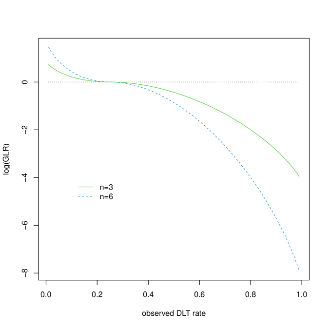
Figure 1: $\log(\text{GLR})$ as a function of the observed DLT rate ($\widehat{p}$) with $\phi=0.25$ and $n=3,6$. The dotted horizontal line corresponds to $\log(\text{GLR})=0$ or, equivalently, $\text{GLR}=1$.

Although $\widehat{p}$ is a discrete random variable, the GLR can be regarded as a continuous function of $\widehat{p}$. Differentiating $\log(\text{GLR})$ with respect to $\widehat{p}$ shows that the GLR is a decreasing function of $\widehat{p}$. The rate at which $\log(\text{GLR})$ decreases with $\widehat{p}$ is proportional to $n$. Figure 1 displays some examples of $\log(\text{GLR})$ as a function of $\widehat{p}$.

Table 1 shows GLR values for some common choices of $n$ (3–6) and $\phi$ (0.2, 0.25 and 0.3). In these scenarios, the only way to obtain strong evidence in either direction ($\text{GLR}\geq 32$ or $\leq 1/32$) is when most patients in a cohort have DLT events, in which case $H_{2}$ is strongly supported over $H_{1}$. The best possible evidence to support $H_{1}$ over $H_{2}$, corresponding to $x=0$, is typically weak ($\text{GLR}<8$) with only one exception ($n=6$, $\phi=0.3$), where it narrowly meets Royal’s benchmark for moderate evidence. For intermediate values of $x$, the GLR is typically between 2 and $1/2$. For example, with one out of six patients experiencing DLT events, the GLR supporting $H_{1}$ over $H_{2}$ ranges between 1.02 and 1.33 as $\phi$ ranges between 0.2 and 0.3. These results indicate that one has to be realistic about how much evidence to expect in a typical dose-finding study.

The GLL suggests the following dose transition rule based on the GLR:

• Escalate if $\text{GLR}\geq k_{1}$;

• De-escalate if $\text{GLR}\leq 1/k_{2}$;

• Stay if $1/k_{2}<\text{GLR}<k_{1}$.

The cut-points $k_{1}$ and $k_{2}$ represent the levels of evidence required for escalation and de-escalation; they need not be equal and may be chosen on the basis of practical considerations. The sample size of a dose-finding study is typically small (3–9 per dose), which suggests that $k_{1}$ and $k_{2}$ cannot be too large. If incorrect escalation is considered more severe than incorrect de-escalation, one may choose $k_{1}>k_{2}$, which indicates that more evidence is required for escalation than for de-escalation. Because the GLR is a decreasing function of $\widehat{p}$, the GLR-based transition rule leads to an interval design where small values of $\widehat{p}$ lead to escalation, large values to de-escalation, and intermediate values to a “stay” decision. Different interval designs (e.g., BOIN and TEQR) can often be calibrated to match or mimic each other by choosing appropriate parameter values. Likewise, the GLR-based design can be related to the other interval designs by calculating GLRs at decision boundaries for the other designs. In this manner, the GLR-based design gives a likelihood interpretation to each existing interval design and provides a unified framework in which different interval designs with the same target DLT rate can be compared directly in terms of how much evidence is required for dose escalation and de-escalation.

For the same choices of $(n,\phi)$ considered in Table 1, Table 2 reports the “effective” values of $(k_{1},k_{2})$ of the 3+3 and various interval designs, regarded as GLR-based designs with the same target DLT rate and the same decision boundaries in $\widehat{p}$. The 3+3 design is not really an interval design; it does not have a clearly stated target DLT rate or precisely defined decision boundaries in $\widehat{p}$. To ease the comparison, for each given value of $\phi$, I use the results in Table 1 to determine the ranges of possible values of $(k_{1},k_{2})$ for GLR-based designs that make the same decisions as the 3+3 design for $n=3$ and $n=6$. The BOIN, TEQR and i3+3 designs have well-defined decision boundaries in $\widehat{p}$, which are substituted into equation (2) to compute $(k_{1},k_{2})$. By replacing $x$ with $n\widehat{p}$ in the posterior distribution of $p$, the mTPI design can be extended easily to accommodate a continuous $\widehat{p}$ and thus can be treated in the same manner. For the BOIN design, I set $\phi_{1}=0.6\phi$ and $\phi_{2}=1.4\phi$ as recommended by Liu and Yuan (2015). For the TEQR, mTPI and i3+3 designs, the equivalence interval is chosen to be $(\phi-0.05,\phi+0.05)$, consistent with common practice. A uniform prior is used in the mTPI design.

In Table 2, all values of $(k_{1},k_{2})$ are below 2, and most are below 1.5, representing a much lower level of evidence than what is commonly expected in phase III trials ($k=6.82$; Zhang and Zhang, 2013, Section 5). The lower requirement may be appropriate for the objective of the study (dose finding as opposed to hypothesis testing) and the typically small sample size. The likelihood interpretation of the 3+3 design depends heavily on the target DLT rate ($\phi$). With $\phi=0.2$, the design requires more evidence for de-escalation than for escalation. With $\phi=0.3$, it does the opposite. With $\phi=0.25$, it requires similar amounts of evidence for escalation and de-escalation. The BOIN and TEQR designs have similar values of $(k_{1},k_{2})$, which are quite close to 1, and both designs require similar amounts of evidence for escalation and de-escalation, regardless of $\phi$. The mTPI and i3+3 designs are similar in that both require much more evidence for de-escalation than for escalation. For escalation, the requirement of i3+3 is lower than that of mTPI and similar to those of BOIN and TEQR.

By setting a higher bar for de-escalation than for escalation, the mTPI and i3+3 designs tend to be aggressive in moving toward higher doses. This has a potential impact on patient safety, which will be examined in a simulation study. It seems difficult to imagine a general rationale for requiring more evidence for de-escalation than for escalation. In fact, from a patient safety perspective, there is a good rationale for requiring more evidence for escalation than for de-escalation. DLT events are serious events, and it would be advisable to use some caution in dose escalation. No design in Table 2 consistently requires more evidence for escalation than for de-escalation. Although some designs can be modified to produce that effect (e.g., by specifying an asymmetric equivalence interval), such a modification would be ad hoc and unintuitive. In the GLR-based design, one can achieve that goal in a transparent way, by simply setting $k_{1}>k_{2}$. This possibility will be explored in the simulation study.

2.4 GLR Based on Joint Likelihood

The single-dose likelihood used in Section 2.3 is based on observed DLT data at one dose only. Let us now consider a joint likelihood that borrows information across doses under an isotonic regression model. Suppose we have collected DLT data for the first $d$ doses: $\{(n_{i},x_{i}):i=1,\dots,d\}$, where $n_{i}$ is the number of patients treated at dose $i$ and $x_{i}$ is the number of patients who experienced DLT events. Write $\boldsymbol{p}=(p_{1},\dots,p_{d})^{\prime}$, where $p_{i}$ is the true DLT rate of dose $i\in\{1,\dots,d\}=:[d]$. The isotonic regression model assumes that $p_{1}\leq p_{2}\leq\cdots\leq p_{d}$. The joint likelihood for $\boldsymbol{p}$ is simply a product of dose-specific binomial likelihoods:

$$L(\boldsymbol{p})=\prod_{i=1}^{d}p_{i}^{x_{i}}(1-p_{i})^{n_{i}-x_{i}}.$$

Maximizing $L(\boldsymbol{p})$ over $\mathcal{P}=\{\boldsymbol{p}:0\leq p_{1}\leq\cdots\leq p_{d}\leq 1\}$ yields a constrained maximum likelihood estimate of $\boldsymbol{p}$, say $\widetilde{\boldsymbol{p}}=(\widetilde{p}_{1},\dots,\widetilde{p}_{d})^{\prime}$, which can be used to estimate the MTD at the end of the study. Specifically, the estimated MTD is $\max\{i\in[d]:\widetilde{p}_{i}\leq\phi\}$, which is set to 0 if there is no qualifying $i$.

For the current dose $c\in[d]$, we need to compare two competing hypotheses:

$$H_{1c}:p_{c}\leq\phi\qquad\text{versus}\qquad H_{2c}:p_{c}>\phi.$$

The GLR for comparing $H_{1c}$ with $H_{2c}$ is $\sup_{H_{1c}}L(\boldsymbol{p})/\sup_{H_{2c}}L(\boldsymbol{p})$, where

$$\sup_{H_{1c}}L(\boldsymbol{p}) =\max\{L(\boldsymbol{p}):\boldsymbol{p}\in\mathcal{P},p_{c}\leq\phi\},$$

$$\sup_{H_{2c}}L(\boldsymbol{p}) =\max\{L(\boldsymbol{p}):\boldsymbol{p}\in\mathcal{P},p_{c}\geq\phi\}$$

The maximizations involved here and in finding $\widetilde{\boldsymbol{p}}$ are convex optimization problems with linear inequality constraints, which can be solved using an adaptive barrier algorithm (available in R as constrOptim()). Once computed, the GLR can be compared to $(k_{1},k_{2})$ to make a dose transition decision, in the same manner as in Section 2.3.

3 Results

This section reports a simulation study comparing four commonly used interval designs (BOIN, TEQR, mTPI and i3+3) and some GLR-based designs with $k_{1}>k_{2}$. The BOIN design is implemented with the default settings: $\phi_{1}=0.6\phi$ and $\phi_{2}=1.4\phi$. The TEQR, mTPI and i3+3 designs are implemented with the same equivalence interval: $(\phi-0.05,\phi+0.05)$. The uniform prior is used in the mTPI design. The GLR-based designs have $k_{1}=1.5$ and $k_{2}=1.05$ or 1.1, chosen to represent the “opposite” of the mTPI and i3+3 designs in the sense that more evidence is required for escalation than for de-escalation. The GLRs may be based on the single-dose likelihood or the joint likelihood under an isotonic regression model; these are denoted by GLR.sd and GLR.iso, respectively, where a distinction needs to be made. All designs start at the lowest dose and include some form of overdose control. For the existing designs, a dose (and all higher doses) will be eliminated if $\operatorname{P}(p>\phi|n,x)>0.95$ under a uniform prior for $p$, as suggested by Liu and Yuan (2015). For the GLR-based designs, the condition for dose elimination is $\text{GLR}\leq 1/3.87$, equivalent to a significant LR test at $\alpha=0.05$ with $H_{1}:p\leq\phi$ as the null hypothesis. For all designs, MTD estimation is performed by applying the constrained maximum likelihood estimation procedure in Section 2.4 to all available data at the end of the study.

In this simulation study, the cohort size is fixed at 3, the total number of doses is $D\in\{4,6,8\}$, and for each value of $D$ the maximum number of cohorts is $M=2D$ (i.e., 2 cohorts per dose on average). The target DLT rate is $\phi\in\{0.2,0.25,0.3\}$. Given $\phi$ and $D$, the true DLT rates, $\boldsymbol{p}=(p_{1},\dots,p_{D})^{\prime}$, are ordered values in a random sample of size $D$ from the uniform distribution on $(0,2\phi)$, to be generated anew for each trial. Figure 2 shows a random sample of 10 realizations of $\boldsymbol{p}$ with $D=6$ and $\phi=0.25$. Given $\phi$ and $\boldsymbol{p}$, the true MTD is defined as $\max\{i\in[D]:p_{i}\leq\phi\}$, with the understanding that the maximum of an empty set is 0. In each scenario defined by $(D,\phi)$, a total of $10^{4}$ trials are simulated for each design.

The different designs are compared using three metrics. The first one is %MTD, the percentage of trials that correctly find the MTD, which may be 0. The second one is %OT, the percentage of patients who are over-treated (i.e., treated at a dose above the true MTD). The last one is $N_{\text{ave}}$, the average number of patients treated, which may be less than $N_{\max}=3M=6D$ due to the possibility of early stopping. The three metrics represent, respectively, the accuracy of MTD estimation, the extent of over-treatment, and the cost of the study.

Table 3 presents a summary of simulation results based on the three metrics defined above. In general, %MTD increases with $\phi$ and decreases with $D$. In each scenario, the different designs perform similarly in terms of %MTD and $N_{\text{ave}}$, but there are substantial differences in %OT. At $\phi=0.2$, the %OT values are clearly larger (by 3–8 percentage points) for the mTPI and i3+3 designs than for the BOIN and TEQR designs. At $\phi=0.25$, the differences become smaller in some cases but largely persist. At $\phi=0.3$, the four designs are virtually indistinguishable in %OT. It is worth noting that the GLR-based designs consistently produce smaller %OT values than all of the other four designs. The amount of improvement (i.e., decrease in %OT) is substantial in all scenarios and particularly large at $\phi=0.3$. Among the GLR-based designs, differences are generally small and inconsistent, with one notable exception: at $\phi=0.25$, increasing $k_{2}$ from 1.05 to 1.1 with $k_{1}$ fixed at 1.5 leads to a slight increase in %MTD and a larger increase in %OT. In other scenarios, the two configurations produce similar results. The results are also similar between GLR.sd and GLR.iso. It is not clear that using the join likelihood instead of the single-dose likelihood leads to improved performance.

4 Discussion

This article provides a new perspective on dose transition rules in dose-finding studies that aim to find the MTD. In this perspective, the key scientific question is whether the true DLT rate of the current dose exceeds the target DLT rate, and the statistical question is how to evaluate the statistical evidence in the available DLT data with respect to that scientific question. According to the GLL, the GLR can be used as a measure of statistical evidence and as the basis for making dose transition decisions. This leads to a GLR-based dose transition rule that can be used to interpret and compare existing interval designs and construct new ones. A GLR-based comparison of commonly used versions of the BOIN, TEQR, mTPI and i3+3 designs indicates that, unlike the first two designs, the last two designs require more evidence for de-escalation than for escalation, which raises concerns about patient safety. Simulation results confirm that the last two designs frequently produce higher proportions of over-treated patients. These observations motivate the consideration of GLR-based designs that require more evidence for escalation than for de-escalation, which are shown in the simulation study to reduce the proportion of over-treated patients while maintaining the accuracy of MTD estimation.

It is somewhat disappointing that, compared to the single-dose likelihood, the joint likelihood based on an isotonic regression model does not appear to enhance the performance of GLR-based designs. From a practical point of view, this is actually good news as the GLR based on the single-dose likelihood is easy to compute and the resulting dose transition rule can be tabulated before starting a study. Computing the GLR based on the joint likelihood is more difficult and requires special software, and the computation has to be conducted in real time if one chooses to use this GLR in a study. These observations together support the use of the single-dose likelihood in practice.

While this article is focused on toxicity assessment, the GLL can also be used to address research questions related to drug activity. There is an ongoing effort to formulate statistical hypotheses on drug activity, derive and compute the corresponding GLRs, and develop dose transition rules that take both toxicity and activity into account.

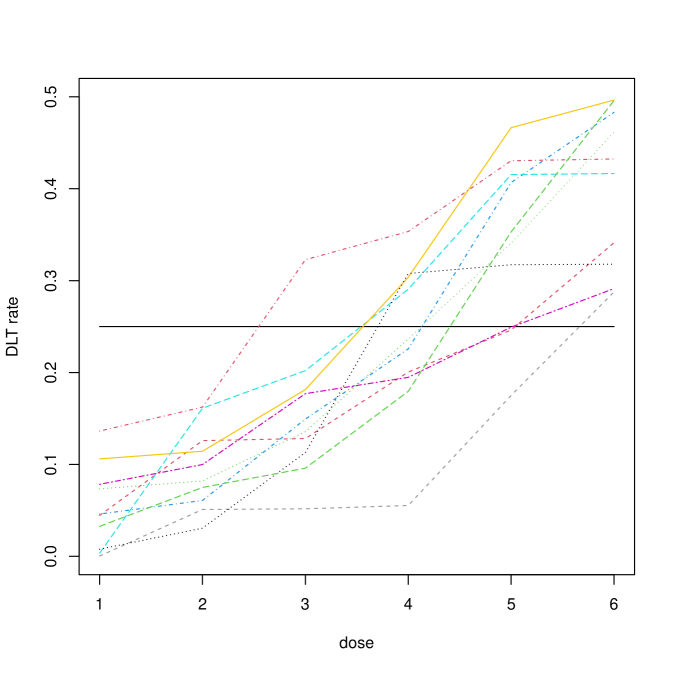
Figure 2: 10 sets of true DLT rates at $D=6$ doses, generated randomly as in the simulation study (see Section 3 for details). The solid horizontal line corresponds to the target DLT rate ($\phi=0.25$).

Table 1: GLR values for comparing $H_{1}:p\leq\phi$ with $H_{2}:p>\phi$ in the situation of Section 2.3 with common choices of $n$ and $\phi$. GLR values greater than 1 support $H_{1}$ over $H_{2}$. GLR values less than 1, which support $H_{2}$ over $H_{1}$, are expressed as reciprocals to indicate the strength of support.

$n$	$x$	$\phi$
		0.2	0.25	0.3
3	0	1.95	2.37	2.92
	1	1/1.16	1/1.05	1/1.01
	2	1/4.63	1/3.16	1/2.35
	3	$<1/100$	1/64.0	1/37.0
4	0	2.44	3.16	4.16
	1	1/1.03	1.00	1.02
	2	1/2.44	1/1.78	1/1.42
	3	1/16.5	1/9.0	1/5.58
	4	$<1/100$	$<1/100$	$<1/100$
5	0	3.05	4.21	5.95
	1	1.00	1.04	1.14
	2	1/1.69	1/1.31	1/1.12
	3	1/6.75	1/3.93	1/2.61
	4	1/64.0	1/28.0	1/14.4
	5	$<1/100$	$<1/100$	$<1/100$
6	0	3.81	5.62	8.50
	1	1.02	1.13	1.33
	2	1/1.34	1/1.11	1/1.02
	3	1/3.81	1/2.37	1/1.69
	4	1/21.4	1/9.99	1/5.53
	5	$<1/100$	1/91.4	1/39.4
	6	$<1/100$	$<1/100$	$<1/100$

Table 2: Effective values of $(k_{1},k_{2})$ for the 3+3 and various interval designs, regarded as GLR-based designs with the same target DLT rate ($\phi$) and the same decision boundaries in $\widehat{p}$ (see Section 2.3 for details).

Design	$n$	$\phi=0.2$			$\phi=0.25$			$\phi=0.3$
		$k_{1}$	$k_{2}$		$k_{1}$	$k_{2}$		$k_{1}$	$k_{2}$
3+3		1.00–1.02	1.16–1.34		1.00–1.13	1.05–1.11		1.00–1.33	1.01–1.02
BOIN	3	1.02	1.01		1.02	1.02		1.03	1.02
	4	1.02	1.02		1.03	1.02		1.04	1.03
	5	1.03	1.02		1.04	1.03		1.05	1.04
	6	1.04	1.03		1.05	1.04		1.06	1.05
TEQR	3	1.03	1.02		1.02	1.02		1.02	1.02
	4	1.03	1.03		1.03	1.03		1.02	1.02
	5	1.04	1.04		1.04	1.03		1.03	1.03
	6	1.05	1.05		1.04	1.04		1.04	1.04
mTPI	3	1.10	1.54		1.13	1.47		1.15	1.42
	4	1.13	1.68		1.16	1.61		1.20	1.54
	5	1.16	1.82		1.20	1.73		1.24	1.65
	6	1.19	1.95		1.24	1.84		1.28	1.75
i3+3	3	1.03	1.83		1.02	1.73		1.02	1.67
	4	1.03	1.52		1.03	1.46		1.02	1.42
	5	1.04	1.36		1.04	1.31		1.03	1.28
	6	1.05	1.25		1.04	1.22		1.04	1.20

Table 3: Summary of simulation results: percentage of trials that correctly find the MTD (%MTD), percentage of patients who are over-treated (%OT), and average number of patients treated ($N_{\text{ave}}$) for four commonly used interval designs and some GLR-based designs with $k_{1}>k_{2}$ in various scenarios defined by the total number of doses ($D$) and the target DLT rate ($\phi$) (see Section 3 for details).

$D$	Design	$k_{1}$	$k_{2}$	$\phi=0.2$				$\phi=0.25$				$\phi=0.3$
				%MTD	%OT	$N_{\text{ave}}$		%MTD	%OT	$N_{\text{ave}}$		%MTD	%OT	$N_{\text{ave}}$
4	BOIN			48.1	33.5	23.1		51.8	34.3	23.7		55.3	38.0	23.4
	TEQR			47.6	34.4	23.1		50.7	34.4	23.6		55.3	37.6	23.5
	mTPI			48.3	40.6	23.1		52.2	37.2	23.7		56.1	38.4	23.5
	i3+3			48.1	38.0	23.1		51.1	41.1	23.6		55.7	37.3	23.5
	GLR.sd	1.5	1.05	46.6	31.4	23.3		51.5	29.0	23.6		56.5	31.2	23.6
	GLR.sd	1.5	1.1	47.8	31.2	23.2		52.6	32.7	23.6		56.1	31.4	23.6
	GLR.iso	1.5	1.05	46.8	30.5	23.2		51.8	28.9	23.7		56.4	31.1	23.6
	GLR.iso	1.5	1.1	47.7	31.0	23.2		52.5	32.2	23.7		56.3	30.9	23.6
6	BOIN			38.8	28.1	35.3		43.5	28.4	35.8		47.3	32.2	35.6
	TEQR			39.0	28.7	35.3		42.5	28.4	35.7		48.1	32.9	35.6
	mTPI			38.5	35.2	35.2		43.9	31.3	35.8		47.0	32.8	35.6
	i3+3			39.1	33.0	35.3		44.2	35.3	35.8		47.9	32.9	35.6
	GLR.sd	1.5	1.05	39.4	24.9	35.4		42.8	22.8	35.8		48.6	25.2	35.7
	GLR.sd	1.5	1.1	39.0	25.2	35.4		44.4	25.8	35.8		47.9	25.2	35.7
	GLR.iso	1.5	1.05	39.9	24.3	35.4		43.4	22.9	35.7		46.7	25.0	35.7
	GLR.iso	1.5	1.1	39.3	24.9	35.4		43.7	26.4	35.8		48.3	25.4	35.7
8	BOIN			33.2	24.2	47.3		36.9	25.6	47.8		40.6	28.5	47.8
	TEQR			33.7	25.2	47.3		36.1	25.5	47.8		40.9	29.4	47.7
	mTPI			33.5	31.1	47.4		37.1	26.7	47.9		41.3	28.1	47.8
	i3+3			33.4	28.9	47.5		36.6	31.7	47.8		41.2	29.0	47.8
	GLR.sd	1.5	1.05	32.8	20.8	47.4		35.3	18.4	47.8		39.7	21.1	47.8
	GLR.sd	1.5	1.1	32.7	21.1	47.4		36.6	22.0	47.8		40.7	21.0	47.8
	GLR.iso	1.5	1.05	33.9	20.2	47.5		36.8	18.5	47.8		40.4	20.1	47.8
	GLR.iso	1.5	1.1	33.9	21.0	47.5		39.0	22.1	47.9		41.5	21.1	47.8

References

- Ananthakrishnana et al. (2018) Ananthakrishnana R, Greenb S, Li D, LaValleya M (2018). Extensions of the mTPI and TEQR designs to include non-monotone efficacy in addition to toxicity for optimal dose determination for early phase immunotherapy oncology trials. Contemporary Clinical Trials Communications, 10, 62–76.
- Aout and Seroutou (2018) Aout M, Seroutou A (2018). Joint modelling of efficacy and toxicity in the dose escalation phase I studies. Open Journal of Statistics, 8, 603–613.
- Bickel (2008) Bickel DR (2008). The strength of statistical evidence for composite hypotheses with an application to multiple comparisons. COBRA Preprint Series, Article 49 (available online at http://biostats.bepress.com/cobra/ps/art49).
- Blanchard and Longmate (2011) Blanchard MS, Longmate JA (2011). Toxicity equivalence range design (TEQR): a practical Phase I design. Contemporary Clinical Trials, 32, 114–121.
- Blume (2002) Blume JD (2002). Likelihood methods for measuring statistical evidence. Statistics in Medicine, 21, 2563–2599.
- Chiuzan et al. (2018) Chiuzan C, Garrett-Mayer E, Nishimura MI (2018). An adaptive dose-finding design based on both safety and immunologic responses in cancer clinical trials. Statistics in Biopharmaceutical Research, 10, 185–195.
- Chiuzan et al. (2015) Chiuzan C, Garrett-Mayer E, Yeatts S (2015). A Likelihood-based approach for computing the operating characteristics of the 3+3 phase I clinical trial design with extensions to other A+B Designs. Clinical Trials, 12, 24–33.
- Cook et al. (2015) Cook N, Hansena AR, Siu LL, Razak ARA (2015). Early phase clinical trials to identify optimal dosing and safety. Molecular Oncology, 9, 997–1007.
- FDA (2023) Food and Drug Administration (2023). Optimizing the dosage of human prescription drugs and biological products for the treatment of oncologic diseases. Available online at https://www.fda.gov/media/164555/download.
- Hacking (1965) Hacking I (1965). Logic of Statistical Inference. Cambridge University Press, New York.
- Ji et al. (2010) Ji Y, Liu P, Li Y, Bekele BN (2010). A modified toxicity probability interval method for dose-finding trials. Clinical Trials, 7, 653–663.
- Korn et al. (1994) Korn EL, Midthune D, Chen TT, Rubinstein LV, Christian LC, Simon RM (1994). A comparison of two phase I trial designs. Statistics in Medicine, 13, 1799–1806.
- Li et al. (2016) Li DH, Whitmore JB, Guo W, Ji Y. Toxicity and efficacy probability interval design for phase I adoptive cell therapy dose-finding clinical trials. Clinical Cancer Research, 23, 13–20.
- Lin et al. (2020) Lin R, Zhou Y, Yan F, Li D, Yuan Y (2020). BOIN12: Bayesian optimal interval phase I/II trial design for utility-based dose finding in immunotherapy and targeted therapies. Journal of Clinical Oncology – Precision Medicine, 4, 1393–1402.
- Liu et al. (2020) Liu M, Wang SJ, Ji Y (2020). The i3+3 design for phase I clinical trials. Journal of Biopharmaceutical Statistics, 30, 294–304.
- Liu and Yuan (2015) Liu S, Yuan Y (2015). Bayesian optimal interval designs for phase I clinical trials. Journal of the Royal Statistical Society, Series C (Applied Statistics), 64, 507–523.
- O’Quigley et al. (1990) O’Quigley J, Pepe M, Fisher L (1990). Continual reassessment method: A practical design for phase 1 clinical trials in cancer. Biometrics, 46, 33–48.
- Royall (1997) Royall R (1997). Statistical Evidence: A Likelihood Paradigm. Chapman & Hall, Boca Raton, FL.
- Shah et al. (2021) Shah M, Rahman A, Theoret MR, Pazdur R (2021). The drug-dosing conundrum in oncology — when less is more. New England Journal of Medicine, 385, 1445–1447.
- Simon et al. (1997) Simon R, Freidlin B, Rubinstein L, Arbuck SG, Collins J, Christian MC (1997). Accelerated titration designs for phase I clinical trials in oncology. Journal of the National Cancer Institute, 89, 1138–1147.
- Storer (1989) Storer BE (1989). Design and analysis of phase I clinical trials. Biometrics, 45, 925–937.
- Takeda et al. (2018) Takeda T, Taguri M, Morita S (2018). BOIN‐ET: Bayesian optimal interval design for dose finding based on both efficacy and toxicity outcomes. Pharmaceutical Statistics, 17, 383–395.
- Wages et al. (2018) Wages NA, Chiuzan C, Panageas KS (2018). Design considerations for early-phase clinical trials of immune-oncology agents. Journal for ImmunoTherapy of Cancer, 6:81 (doi: 10.1186/s40425-018-0389-8).
- Wages and Tait (2015) Wages NA, Tait C (2015). Seamless phase I/II adaptive design for oncology trials of molecularly targeted agents. Journal of Biopharmaceutical Statistics, 25, 903–920.
- Zang et al. (2014) Zang Y, Lee JJ, Yuan Y (2014). Adaptive designs for identifying optimal biological dose for molecularly targeted agents. Clinical Trials, 11, 319–327.
- Zhang and Zhang (2013) Zhang Z, Zhang B (2013). A likelihood paradigm for clinical trials (with discussion and rejoinder). Journal of Statistical Theory and Practice, 7, 157–177.