Short-range interactions are irrelevant at the quasiperiodic-driven Luttinger Liquid to Anderson Glass transition

Abstract

We show that short-range interactions are irrelevant around gapless ground-state delocalization-localization transitions driven by quasiperiodicity in interacting fermionic chains. In the presence of interactions, these transitions separate Luttinger Liquid and Anderson glass phases. Remarkably, close to criticality, we find that excitations become effectively non-interacting. By formulating a many-body generalization of a recently developed method to obtain single-particle localization phase diagrams, we carry out precise calculations of critical points between Luttinger Liquid and Anderson glass phases and find that the correlation length critical exponent takes the value $\nu=1.001\pm 0.007$, compatible with $\nu=1$ known exactly at the non-interacting critical point. We also show that other critical exponents, such as the dynamical exponent $z$ and a many-body analog of the fractal dimension are compatible with the exponents obtained at the non-interacting critical point. Noteworthy, we find that the transitions are accompanied by the emergence of a many-body generalization of previously found single-particle hidden dualities. Finally, we show that in the limit of vanishing interaction strength, all finite range interactions are irrelevant at the non-interacting critical point.

There has been a continued interest in the effects of quasiperiodicity on quantum many body systems thanks to their experimental accessibility in ultracold atoms and trapped ions (Boers et al., 2007; Roati et al., 2008; Modugno, 2009; Schreiber et al., 2015; Lüschen et al., 2018; Yao et al., 2019, 2020; Gautier et al., 2021; An et al., 2021; Kohlert et al., 2019) and most recently moiré materials (Balents et al., 2020). From a theoretical point of view, the effects of interactions on Anderson insulating ground states is also of paramount importance in the context of many-body localization, where random and quasiperiodic systems have important and fundamental differences that are currently under intense scrutiny (Khemani et al., 2017; Setiawan et al., 2017; Chandran and Laumann, 2017; Agrawal et al., 2020). Of paramount importance is understanding the nature of such many body localization phase transitions that take place at finite energy density far away from the ground state (Iyer et al., 2013; Mondaini and Rigol, 2015; Modak and Mukerjee, 2015; Lee et al., 2017; Žnidarič and Ljubotina, 2018; Xu et al., 2019; Doggen and Mirlin, 2019; Vu et al., 2022; Aramthottil et al., 2021). However, even in the limit of the ground state, the nature of the universality class of the interacting quasiperiodic electronic “glass” transition has remained poorly understood.

A great deal of understanding has been achieved in non-interacting quasiperiodic systems thanks to rigorous results on the paradigmatic Aubry-André model (Aubry and André, 1980; Avila and Jitomirskaya, ; Szabó and Schneider, 2018; Cookmeyer et al., 2020), where an energy-independent delocalization-localization takes place, and on its generalizations to phase diagrams that contain mobility edges and/or critical phases (Johansson and Riklund, 1991; Biddle and Das Sarma, 2010; Bodyfelt et al., 2014; Liu et al., 2015; Danieli et al., 2015; Ganeshan et al., 2015; Liu et al., 2022). However, the interplay between quasiperiodicity and interactions has been less explored. Typically, the studies on this interplay are in the context of many-body localization, for highly excited states in the middle of the many-body spectrum (Iyer et al., 2013; Mondaini and Rigol, 2015; Modak and Mukerjee, 2015; Lee et al., 2017; Žnidarič and Ljubotina, 2018; Xu et al., 2019; Doggen and Mirlin, 2019; Vu et al., 2022; Aramthottil et al., 2021). An equally interesting direction is the study of ground-state localization properties (Vidal et al., 1999; Schuster et al., 2002; Roux et al., 2008; Kraus et al., 2014; Naldesi et al., 2016; Cookmeyer et al., 2020; Vu and Das Sarma, 2021; Chandran and Laumann, 2017; Crowley et al., 2018; Agrawal et al., 2020; Crowley et al., 2022; Vu and Das Sarma, 2021, 2022). Deep enough in the localized phase, upon adding nearest-neighbor interactions to Aubry-André model, the ground-state remains localized, giving rise to an Anderson glass (AG) phase (Schuster et al., 2002; Naldesi et al., 2016; Mastropietro, 2017; Cookmeyer et al., 2020). On the other hand, at weak interaction strength the Luttinger liquid (LL) phase is stable towards the inclusion of a sufficiently weak quasiperiodic potential (Vidal et al., 2001; Naldesi et al., 2016). The gapless ground-state delocalization-localization transition therefore persists in the presence of interactions, corresponding to a transition between the LL and AG phases. The critical properties of the LL-AG transition were studied in detail for the non-interacting Aubry-André model (Szabó and Schneider, 2018; Wei, 2019; Cookmeyer et al., 2020), and it was proposed in (Cookmeyer et al., 2020) that nearest-neighbor repulsive interactions may be irrelevant at the critical point. In more generic interacting models beyond the paradigmatic Aubry-André model, the ground-state localization properties remain largely unexplored.

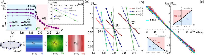
Figure 1: Quantum phase transition between Luttinger liquid (LL) and Anderson glass (AG) phases. (a) The many-body localization tensor $\lambda_{xx}^{2}$, as given in Eq. 3 and computed using open boundary conditions for different system sizes $N$, is plotted versus the quasiperiodic potential strength $V$, for the model in Eq. 1 with $V_{2}=0.25,t_{2}=0.2,U=0.5$ and $U_{2}=0.4$. The scaling of the $\phi$-averaged charge gap with system size (see Eq. 4 and Fig. 3(c) for definition and additional details) in the LL phase (for $V=1.65$) and at the critical point (indicated by the vertical dashed line) is shown in the inset, unveiling a non-Lorentz-invariant critical point (with dynamical critical exponent $z>1$). The blue and green dashed lines show the scaling behaviour known for the non-interacting Aubry-André model, respectively at extended and critical points, which is compatible with the scaling behaviour observed at the LL phase and the interacting critical point. Below these figures, we show the $E_{\text{GS}}(\varphi,\kappa)$ contours for a periodic system with a threaded flux $\kappa$ (illustrated in the bottom left figure), for $N=41$, at representative points in the LL (i) and AG (iii) phases, and at the self-dual point (ii), that approaches the critical point (whose estimation is shown by the vertical dashed line) as $N\rightarrow\infty$. $(\varphi_{0},\kappa_{0})$ in these figures is chosen so that $E_{\text{GS}}(\varphi_{0},\kappa_{0})$ is minimum. (b) $\delta E_{\kappa\varphi}$ defined in Eq. 2 (using $\delta s=\pi/20$) for (A): model 1 (see main text bellow Eq. 1), with $U=-1$; (B) Aubry-André model (C) model 2 with $U_{2}=-0.4$, for $L=\{17\textrm{(red)},41\textrm{(blue)},99\textrm{(green)}\}$. (c) Data collapse of $\log\delta E_{\kappa\varphi}$ as a function of $N^{1/\nu}v(N,\bm{\lambda})$, using $\nu=1$, where $\bm{\lambda}$ contains the model parameters, $v(N,\bm{\lambda})=[V-V_{c}(N,\bm{\lambda})]/V_{c}(N,\bm{\lambda})$ and $V_{c}(N,\bm{\lambda})$ is the value of $V$ for which $\delta E_{\kappa\varphi}(N,V,\bm{\lambda})=1$. The data was obtained across the LL-AG transitions shown in the insets, for model 1 (right) and model 2 (left). The results for $N=\{17,41,99\}$ correspond to the red, blue and green markers, respectively. In cyan, we show the result for the non-interacting Aubry-André model. The critical points in the insets [as well as the critical point in (a)] are estimated through $V=V_{c}(N=99,\bm{\lambda})\approx V_{c}(\infty,\bm{\lambda})$. The validity of this estimation is confirmed by the small error bars (smaller or of the size of the data points), computed through $|V_{c}(99,\bm{\lambda})-V_{c}(41,\bm{\lambda})|$.

In this paper we show that interactions are irrelevant around quasiperiodicity-driven LL-AG transitions for a broad class of non-interacting and interacting generalizations of the Aubry-André model, that include next-nearest-neighbor hoppings and interactions and an additional quasiperiodic potential. In particular, we show that the excitations become effectively non-interacting around these transitions and provide solid evidence that the addition of interactions does not affect any of the (infinite number of) critical exponents obtained in the non-interacting limit, although they modify non-universal properties, e.g. the location of the critical point. Remarkably, we also find that many-body generalizations of the single-particle dualities discovered for widely different 1D models (Gonçalves et al., 2022a; Biddle and Das Sarma, 2010; Ganeshan et al., 2015) emerge around criticality. We present a scaling argument based on the perturbative effects of interactions at the Aubry-Andre critical point which demonstrates that short-range interactions are irrelevant. The same argument shows that long-range interactions can become relevant.

Our main results are shown in Fig. 1. In Fig. 1(a) we show an example of a LL-AG transition, in which we set all the couplings of our class of models (in Eq. 1 below) different from zero. A way to capture this transition is with the many-body localization length (see Eq. 3 for definition) (Resta and Sorella, 1999; Resta, 2011; Kerala Varma and Pilati, 2015) that diverges (saturates) at the LL (AG) phase due to the extended (localized) nature of the many-body wave function.

One of our main findings in this work is that this transition can also be captured in a precise manner with minimal scaling assumptions, using a many-body generalization of the single-particle theory developed in (Gonçalves et al., 2022a, b). This involves considering periodic approximations of the quasiperiodic system, as illustrated at the bottom left corner of Fig. 1(a), and inserting a flux $\kappa$ through the resulting ring. The localization properties can then be inferred based on how the ground-state energy ($E_{{\rm GS}}$) depends on these fluxes and on real-space shifts between the lattice and origin of the potential that we encode in the variable $\varphi$, as illustrated in Fig. 1(a), as the size of the periodic approximation ($N$) is increased. The quasiperiodic limit is approached for $N\rightarrow\infty$. In Fig. 1(a), we show examples of the energy contours for fixed $N=41$, for different values of $V$. We can see that in the LL (AG) phase, there is a very small dependence on $\varphi$ ($\kappa$), while close to the critical point, there is an equal dependence on both phases. We can make a more quantitative analysis by computing the ratio between the energy dispersions along $\kappa$ and $\varphi$ respectively, $\delta E_{\kappa\varphi}$ (see Eq. 2 for precise definition), for different $N$. Example results are given in Fig. 1(b) for different models, where we can see that $\delta E_{\kappa\varphi}$ diverges (scales to zero) at the LL (AG) phase. This implies that the $\varphi$-($\kappa$-) dependence becomes irrelevant with respect to the $\kappa$-($\varphi$-) dependence at the LL (AG) phases as $N$ increases, and the model flows to a delocalized (localized) fixed-point as defined in (Gonçalves et al., 2022b). Remarkably, at the critical point, $\delta E_{\kappa\varphi}$ approaches unity as $N$ is increased, which implies that the shift and flux dependencies become equivalent. The self-dual point, defined here as the point for which $\delta E_{\kappa\varphi}=1$ , therefore approaches the critical point as $N\rightarrow\infty$, providing a very precise way of estimating it.

With the ansatz $\delta E_{\kappa\varphi}\propto e^{-N/\xi}$, where $\xi\sim|V-V_{c}|^{-\nu}$ is the correlation length, we were able to collapse the results for each model considered here into a single universal curve using the correlation length critical exponent $\nu=1$ known for the non-interacting Aubry-André model, as shown in Fig. 1(c). The obtained scaling function near criticality is in excellent agreement with the one obtained for the non-interacting Aubry-André model, shown in cyan in Fig. 1(c). The good quality of the collapse and further results on additional critical exponents presented throughout the manuscript support the conclusion that around criticality, different interacting and non-interacting models belong to the same non-interacting universality class.

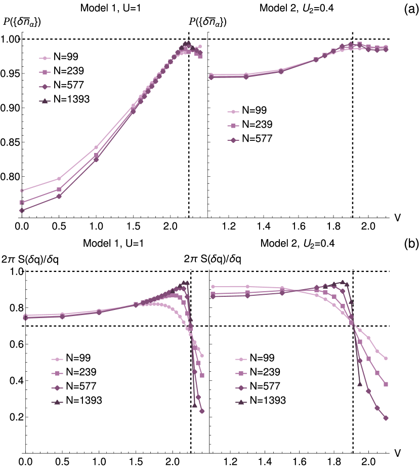
Figure 2: Non-interacting excitations at the critical point. (a) Occupation inverse participation ratio $P(\{\delta\bar{n}_{\alpha}\})$ defined below Eq. 7, and (b) slope of structure factor $S(\delta q)$ for the smallest non-vanishing momentum $\delta q=20\pi/N$ as a function of $V$ for $U=1,\phi=1.123$ and $V_{2}=t_{2}=U_{2}=0$ (left) and $U=0.5,V_{2}=0.25,t_{2}=0.2,U_{2}=0.4$ (right). The vertical dashed line corresponds to the critical point estimated from $\delta E_{\kappa\varphi}$ and the horizontal dashed line is the slope of the linear contribution to $S(q)$ at the critical point (see text).

Models and Methods.—

We study the class of models described by the Hamiltonian

$$H= -t\sum_{i}c_{i}^{\dagger}c_{i+1}-t_{2}\sum_{i}c_{i}^{\dagger}c_{i+2}+{\rm h.c.}$$ (1)

$$+\sum_{i}\Big{(}V\cos(2\pi\tau i+\phi)+V_{2}\cos[2(2\pi\tau i+\phi)]\Big{)}c_{i}^{\dagger}c_{i}$$

$$+U\sum_{i}n_{i}n_{i+1}+U_{2}\sum_{i}n_{i}n_{i+2}$$

where $c_{i}^{\dagger}$ creates a particle at site $i$ and we set $t=1$ throughout the manuscript. The first and third rows contain nearest- and next-nearest-neighbor hoppings and interactions, respectively, while the second row contains quasiperiodic potentials of intensity $V$ and $V_{2}$, with $\tau$ being an irrational number and the phase $\phi$ representing a shift of the potentials with respect to the lattice sites. For the results presented in this manuscript, we set $\tau=1/\sqrt{2}$ (to compare results with Refs. (Cookmeyer et al., 2020; Naldesi et al., 2016)) and work at half-filling $\rho=1/2$ (unless otherwise specified), choosing a number of particles $N_{p}=\lfloor N/2\rfloor$, where $\lfloor x\rfloor$ denotes the integer part of $x$ (the floor function). We have checked that our conclusions do not rely on being at this particular filling, see SM. We choose the following sets of parameters: Aubry-André model with nearest-neighbor interaction, $V_{2}=t_{2}=U_{2}=0$ (model 1) ; generalized Aubry-André model, with $U=0.5,V_{2}=0.25,t_{2}=0.2,U_{2}\neq 0$ (model 2).

To study the models in detail, we computed several different quantities using the DMRG technique (White, 1992; Schollwöck, 2005), as implemented in the iTensor library (Fishman et al., 2020a, b), applying both periodic and open boundary conditions. We required iTensor’s truncation error to be less than $10^{-10}$ and only stopped the sweeping procedure once some convergence requirements were satisfied, up to a maximum of $500$ sweeps. In particular, for twisted boundary conditions, we require the energy variance, $\Delta_{H}=\langle H^{2}\rangle-\langle H\rangle^{2}$, to be below $5\times 10^{-6}$; the ground-state energy difference between two sweeps to be below $\Delta E_{{\rm GS}}=10^{-5}$; and the difference in the entanglement entropy at the middle bond inbetween two sweeps to be below $\Delta S_{{\rm GS}}=10^{-3}$. For open boundary conditions, we require $\Delta_{H}$ at least below $10^{-6}$; $\Delta E_{{\rm GS}}\leq 10^{-7}$; and $\Delta S_{{\rm GS}}\leq 10^{-4}$.

In our finite-size simulations, we use rational approximants of $\tau$, $\tau_{c}=p/N$, with $p$ and $N$ co-prime numbers. These approximants were chosen to be exact convergents of the continued fraction expansion of $\tau$.

Twisted boundary conditions.—

We consider a ring with $N$ sites as illustrated in the bottom left corner of Fig. 1(a) with twisted boundary conditions that corresponds to threading a flux $\kappa$ through the system. This flux can simply be added to the model in Eq. 1 by making the replacement $t\rightarrow te^{ik}$ and $t_{2}\rightarrow t_{2}e^{2ik}$, with $k=\kappa/N$. For the choices $\tau=\tau_{c}$, making shifts $\phi\rightarrow\phi+2\pi/N$ simply corresponds to a relabelling of the indices in this model (Gonçalves et al., 2022b), which implies that the many-body ground-state energy is periodic in $\phi$ with period $\Delta\phi=2\pi/N$. With this in mind, we define the rescaled variable $\varphi=N\phi$ so that $E_{{\rm GS}}(\varphi,\kappa)$ has a period $\Delta\varphi=2\pi$. We define the flux-shift sensitivity, $\delta E_{\kappa\varphi}$, as

$$\delta E_{\kappa\varphi}=\lim_{\delta s\rightarrow 0}\frac{E_{{\rm GS}}(\varphi_{0},\kappa_{0}+\delta s)-E_{{\rm GS}}(\varphi_{0},\kappa_{0})}{E_{{\rm GS}}(\varphi_{0}+\delta s,\kappa_{0})-E_{{\rm GS}}(\varphi_{0},\kappa_{0})}$$ (2)

where $(\varphi_{0},\kappa_{0})$ are defined so that $E(\varphi_{0},\kappa_{0})$ is minimum to ensure that $\delta E_{\kappa\varphi}=1$ at self-dual points . Note that the values of $(\varphi_{0},\kappa_{0})$ can depend on $N$ and on the number of particles $N_{p}$. For the system sizes used in the calculations with periodic boundary conditions and $N_{p}=\lfloor N/2\rfloor$, we found $(\varphi_{0},\kappa_{0})=(0,\pi)$ for $N=17,41$ and $(\varphi_{0},\kappa_{0})=(\pi,0)$ for $N=99$. $\delta E_{\kappa\varphi}$ is the many-body generalization of a similar quantity already introduced for the single-particle eigenenergies of non-interacting quasiperiodic models in (Gonçalves et al., 2022b). In the LL (AG) phase, we expect $\delta E_{\kappa\varphi}\rightarrow\infty$ ($\delta E_{\kappa\varphi}\rightarrow 0$) for increasing $N$. At the critical point, we have $\delta E_{\kappa\varphi}\rightarrow 1$, as we shall see.

It is clear from the $E_{{\rm GS}}(\varphi,\kappa)$ contour plots in Fig. 1 that there is a duality between the LL and AG phases around criticality under switching $(\varphi-\varphi_{0})$ and $(\kappa-\kappa_{0})$. The critical point is the self-dual point of this duality, in which $E_{{\rm GS}}$ is invariant under this exchange. In Ref. (Gonçalves et al., 2022b) we have uncovered similar dualities in the single-particle case and found that they could be traced-back to hidden duality transformations between the single-particle wave functions. Remarkably, in the presence of interactions, a many-body generalization of these duality transformations can still be formulated. In the SM we provide the precise definition and some examples.

Open boundary conditions.—

We also employ open boundary conditions that allow to reach fairly large system sizes (Fishman et al., 2020a, b). In order to carry out a complete study of the LL and AG phases, and of the transition between them, we compute several quantities that we detail below.

The many-body localization length shown in Fig. 1 can be defined as (Resta and Sorella, 1999; Resta, 2011; Kerala Varma and Pilati, 2015)

$$\lambda_{xx}^{2}=(\bra{\Psi}\hat{x}^{2}\ket{\Psi}-\bra{\Psi}\hat{x}\ket{\Psi}^{2})/N_{p},$$ (3)

where $\hat{x}=\sum_{i=1}^{N_{p}}\hat{x}_{i}=\sum_{i=1}^{N}x_{i}c_{i}^{\dagger}c_{i}$ is the many-body position operator and $N_{p}$ is the number of particles. Since it measures the variance of the position operator, it can distinguish between the LL and AG phases: it diverges (saturates) with $N$, due to the extended (localized) nature of the many-body wave function at the LL (AG) phase.

To verify the gapless nature of the transition and obtain the dynamical critical exponent $z$, we also computed the charge gap, defined as

$$\Delta_{c}=E_{{\rm GS}}(N_{p}+1)+E_{{\rm GS}}(N_{p}-1)-2E_{{\rm GS}}(N_{p})\sim N^{-z},$$ (4)

where $E_{{\rm GS}}(N_{p})$ is the ground-state energy for $N_{p}$ particles.

In order to study the scaling of the entanglement in different regions of the phase diagram, we computed the entanglement entropy (Vidal et al., 2003; Amico et al., 2008), defined as

$$\mathcal{S}=-\rm{Tr}[\rho_{A}\log\rho_{A}],\textrm{ }\rho_{A}=\rm{Tr}_{B}\ket{\psi}\bra{\psi},$$ (5)

where we choose the partition $A$ containing the first $N_{A}$ sites of the chain. For a 1D critical system whose continuum limit is a conformal field theory with central charge $c$, we have that (Calabrese and Cardy, 2004)

$$\mathcal{S}=\frac{c}{6}\log\Big{(}\frac{N}{\pi}\sin(\pi N_{A}/N)\Big{)}+C^{\prime}.$$ (6)

This is the expected behaviour at the LL phase (with $c=1$), while at the AG phase, $\mathcal{S}$ becomes non-extensive for large enough $N_{A}$.

To better understand the nature of single-particle excitations we also introduce here the particle-addition correlation matrix, that we define as

$$C_{e}^{ij}=\langle c_{i}^{\dagger}c_{j}\rangle_{N_{p}}-\langle c_{i}^{\dagger}c_{j}\rangle_{N_{p}-1}$$ (7)

where $\langle\rangle_{N_{p}}$ denotes expectation value in the ground-state with $N_{p}$ particles. The eigenvalues and eigenvectors of the particle-addition correlation matrix, $\bm{C}_{e}\ket{\alpha}=\delta\bar{n}_{\alpha}\ket{\alpha}$, with $\alpha=0,\cdots,N-1$, correspond to the occupations and natural orbitals. For a non-interacting system, only a single natural orbital corresponding to the $N_{p}$-th highest-energy single-particle eigenstate labelled as $\ket{\alpha=0}$ is occupied (we have $\delta\bar{n}_{0}=1;\delta\bar{n}_{\alpha>0}=0$). In contrast, in the presence of interactions, a particle that is added to the system redistributes over different natural orbitals. Therefore, the deviations from the expected behaviour of a non-interacting particle can be quantified by inspecting the occupations $\{\delta\bar{n}_{\alpha}\}$. For this purpose, we introduce the occupation inverse participation ratio defined as $P(\{\delta\bar{n}_{\alpha}\})=(\sum_{\alpha}|\delta\bar{n}_{\alpha}|^{2})^{-2}\sum_{\alpha}|\delta\bar{n}_{\alpha}|^{4}$. For a non-interacting (interacting) particle, $P(\{\delta\bar{n}_{\alpha}\})=1$ ($P(\{\delta\bar{n}_{\alpha}\})<1$). We therefore expect that $P(\{\delta\bar{n}_{\alpha}\})$ should approach unity whenever interactions become irrelevant.

The nature of the low-energy excitations can also be inspected by analysing the long wavelength (small $q$) behaviour of the static structure factor defined as $S(q)=N^{-1}\sum_{j,l}[\langle n_{j}n_{l}\rangle-\langle n_{j}\rangle\langle n_{l}\rangle]e^{\textrm{i}q(j-l)}$. In the LL phase, the Luttinger liquid correlation parameter $K$ can be computed through $K=2\pi\lim_{q\rightarrow 0}S(q)/q$ (Ejima et al., 2005; Clay et al., 1999; Ejima and Fehske, 2009; Clay and Hardikar, 2005). In a gapless non-interacting and translationally invariant system, it is easy to show that $K=1$. Inside an (interacting) LL phase, however, $K\neq 1$ in general.

To inspect the localization properties of the many-body wave function, we also computed inverse participation ratios (${\rm IPR}$) (Evers and Mirlin, 2008) for the density fluctuations $\delta n_{i}\equiv C_{e}^{ii}$ and for the most occupied (with $\delta\bar{n}_{\alpha}$ closest to 1) natural orbital that we write as $\ket{\alpha=0}=\sum_{i}\psi_{i}^{(0)}\ket{i}$, where $\ket{i}=c_{i}^{\dagger}\ket{0}$ and $\ket{0}$ is the vacuum:

$$\begin{array}[]{cc}{\rm IPR}(\{\delta n_{i}\})&=(\sum_{i}|\delta n_{i}|)^{-2}\sum_{i}|\delta n_{i}|^{2}\\ {\rm IPR}_{{\rm NO}}(q)&=(\sum_{i}|\psi_{i}^{(0)}|^{2})^{-q}\sum_{i}|\psi_{i}^{(0)}|^{2q}.\end{array}$$ (8)

In the non-interacting limit it is easy to show that $\delta n_{i}=|\psi_{i}^{N_{p}}|^{2}$ and $\psi_{i}^{(0)}=\psi_{i}^{N_{p}}$, where $\psi_{i}^{N_{p}}$ is the amplitude of the $N_{p}$-th single-particle wave function (ordered by increasing eigenenergy) at site $i$. The quantities in Eq. 8 are therefore many-body generalizations of the single-particle IPR (Aulbach et al., 2004) used to study the localization properties of single-particle eigenstates. For the conventional definition of the IPR (with $q=2$ in Eq. 8), we have ${\rm IPR}\sim N^{-D_{2}}$, where $D_{2}$ is the fractal dimension, with $D_{2}=1$ for delocalized states, $D_{2}=0$ for localized states and $0<D_{2}<1$ for critical states. For the generalized version, with $q\neq 0$, we have ${\rm IPR}\sim N^{-\tau(q)}$, with $\tau(q)=D_{q}(q-1)$ and $D_{q}=d$ (with $d$ the system’s dimension) for fully delocalized single-fractal states, while $D_{q}$ is a non-linear function of $q$ for multifractal states.

Universal description around criticality.—

As we previously stated, Fig. 1 shows that the results for the quantity $\delta E_{\kappa\varphi}$ in significantly different models can be collapsed into a single universal scaling function. To obtain the collapse in Fig. 1(c), we first defined the normalized distance to the critical point $v(N,\bm{\lambda})=[V-V_{c}(N,\bm{\lambda})]/V_{c}(N,\bm{\lambda})$, where $\bm{\lambda}=(V_{2},t_{2},U,U_{2})$ contains the model parameters (other than $V$) and $V_{c}(N,\bm{\lambda})$ is the value of $V$ at the self-dual point ($\delta E_{\kappa\varphi}(N,V,\bm{\lambda})=1$). The reason why we use $V_{c}(N,\bm{\lambda})$ and not $V_{c}\equiv V_{c}(\infty,\bm{\lambda})$ is that for smaller systems there can be some dependence of $V_{c}(N,\bm{\lambda})$ on $N$. Such dependence can arise not only from finite-size effects, but also because increasing $N$ also slightly modifies the filling $\rho=N_{p}/N$ (due to $N$ being odd) and the value of $\tau_{c}$ (see table S1 in SM).

Further assuming that

$$\delta E_{\kappa\varphi}\sim e^{-N/\xi}$$ (9)

with $\xi\sim v^{-\nu}(N,\bm{\lambda})$ and extracting $\nu$ from a fit using all the obtained data points, we get a critical exponent $\nu=1.001\pm 0.007$ (see SM). Therefore, we set $\nu=1$ and obtain an excellent collapse shown in Fig. 1(c), around the critical point, i.e. around $v(N,\bm{\lambda})=0$. In the SM we also show that this collapse is not a special feature of half-filling, by also considering the case $\rho=1/3$. We conjecture that the collapse should be observed for any filling that is not commensurate with $\tau$ as defined in (Cookmeyer et al., 2020), i.e., that does not satisfy $\rho=\mod(n\tau_{c},1)$, with $n$ an integer that does not depend on system size. At such commensurate fillings, single-particle gaps are opened for any strength of the quasiperiodic potential.

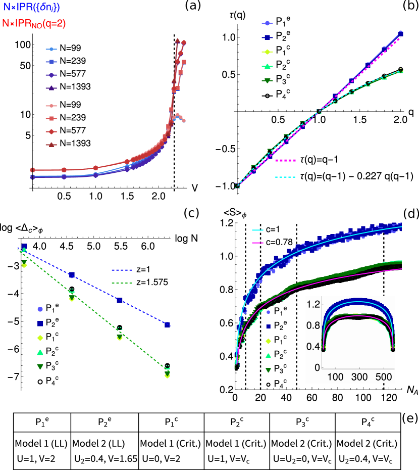
Figure 3: (a) $N{\rm IPR}(\{\delta n_{i}\})$ and $N{\rm IPR}_{{\rm NO}}$ as a function of $V$ for $U=1,\phi=1.123$ and $V_{2}=t_{2}=U_{2}=0$. The vertical dashed line shows the critical point estimated from $\delta E_{\kappa\varphi}$. (b) Exponent $\tau(q)$ defined in Eq. 8 for different models with chosen parameters indicated in table (e), where $P_{i}^{e}$($P_{i}^{c}$) denote extended (critical) points. In table (e), $V_{c}$ corresponds to the estimated critical point. $\tau(q)$ was computed from linear fits to data points $(\log N,\langle{\rm IPR}_{{\rm NO}}(q)\rangle_{\phi})$, where $\langle\rangle_{\phi}$ denotes an average over different choices of $\phi$. We took $\phi_{j}=2\pi j/N_{c},\textrm{ }j=0,\cdots,N_{c}-1$ and $N_{c}\in[100-300]$. We used system sizes $N\in\{99,239,577\}$ for (interacting) points $P_{1}^{e},P_{2}^{e},P_{2}^{c},P_{4}^{c}$ and $N\in\{99,239,577,1393\}$ for (non-interacting) points $P_{1}^{c},P_{3}^{c}$. (c,d) $\langle\Delta_{c}\rangle_{\phi}$ and $\langle\mathcal{S}(N_{A})\rangle_{\phi}$ computed by employing the same averaging procedure used in (b). In (c), the blue and green dashed lines show the scaling behaviour in the non-interacting Aubry-André model, respectively at extended and critical points. In (d), the calculation is done for $N=577$. The main figure shows a close-up at smaller $N_{A}$, while the inset shows the results for all possible $N_{A}$. The vertical dashed lines are guides to the eye for the maxima of the log-periodic oscillations, given by $N_{A}^{(n)}=116/p^{n}$, with $n=0,1,2,3$ and $p=\lim_{m\rightarrow\infty}N_{m}/N_{m+1}=1+\sqrt{2}$. The magenta and cyan curves correspond to fits to Eq. 6 with $c=1$ and $c=0.78$, respectively.

Non-interacting excitations and additional critical exponents.—

We have seen from the quantity $\delta E_{\kappa\varphi}$ in Eq. (2) that the effects of interactions on the scaling function and $\nu$ are irrelevant. We now show that particles become effectively non-interacting in this regime and that the critical properties obtained at different critical points are identical. For the results that follow, we use open boundary conditions.

In Fig. 2(a), we show that the occupation inverse participation ratio approaches $1$ around the critical point. This implies that the single-particle gapless excitations acquire a non-interacting nature. The same conclusion can be drawn by inspecting the behaviour of the Luttinger parameter $K$, in Fig. 2(b). At small $V$, $K$ does not vary significantly (note that when $V=0$, $K$ is known exactly for model 1 (Ejima et al., 2005)). On the other hand, as $V$ gets closer to the critical point, $K$ approaches the non-interacting value $K=1$. Exactly at the different critical points, the system is no longer a LL and at small $q$ we find log-periodic corrections $S(q)\approx 0.7q[1+a\sin(b\log q+\alpha)]$ (see SM). In the AG phase, $S(\delta q)/\delta q$, computed for the smallest non-vanishing momentum $\delta q$, decreases since $S(q)\sim q^{2}$ when $q\rightarrow 0$ [see SM for explicit plots of $S(q)$].

In Fig. 3(a) we show a representative example of the quantities $N\,{\rm IPR}(\{\delta n_{i}\})$ and $N\,{\rm IPR}_{{\rm NO}}$ across the LL-AG transition. We observe LL (AG) phase, is characterized by ${\rm IPR}(\{\delta n_{i}\}),{\rm IPR}_{{\rm NO}}\sim N^{-1}$ ($\sim{\rm const.}$), which is confirmed by the collapse (divergence) of the curves below (above) the transition for different $N$, in direct analogy with the results for the single-particle IPR in the non-interacting case. Note that both quantities become almost quantitatively equal close to the critical point and at the AG phase. At the critical point we expect multifractal scaling with an infinite set of critical exponents (i.e. the multifractal spectrum). Averaging our results over $\phi$, we compute the exponent $\tau_{q}$ defined in Eq. 8, that we show in Fig. 3(b). In this figure, we can see that in the LL phase ($P_{1}^{e}$ and $P_{2}^{e}$), $D_{q}\approx 1$, while at interacting critical points ($P_{2}^{c}$ and $P_{4}^{c}$) we observe a multifractal behaviour quantitatively compatible with the one obtained at the non-interacting critical points ($P_{1}^{c}$ and $P_{3}^{c}$), that is, $D_{q}\approx 1-0.227q$ . In the SM, we show explicit data for $\langle{\rm IPR}_{{\rm NO}}(q)\rangle_{\phi}$ as a function of $N$, from which the exponents $\tau(q)$ were extracted.

We also computed the $\phi$-averaged scaling of the charge gap $\Delta_{c}$ in Fig. 3(c), that allowed us to extract dynamical critical exponents $z$. Remarkably, the scaling exponents are compatible with the exponents obtained for the non-interacting Aubry-André model. This, together with the multifractal analysis, is a strong indication that the universality class of the delocalization-localization transition is unchanged upon the addition of interactions. An important remark is that, as seen in Ref. (Cookmeyer et al., 2020), the dynamical exponent for the non-interacting Aubry-André model can depend on $\rho$ and $\tau$. Since here we are fixing the latter, a natural question is whether the independence of the critical exponents on the model is a special feature of our choice. In the SM, we argue that this is not the case by obtaining compatible finite-size scalings of the charge gap at critical points of different non-interacting models for other choices of $\rho$ and $\tau$.

Finally, we also plot the $\phi$-averaged entanglement entropy as a function of the size of bipartion $A$, $N_{A}$, in Fig. 3(d). In the LL phase, $S$ follows the behaviour of Eq. 6 with $c=1$, as in the non-interacting delocalized case (Ribeiro et al., 2013). At the critical point, the results are compatible with the non-interacting Aubry-André model result, showing corrections to Eq. 6 in the form of log-periodic oscillations, similarly with what was observed for critical aperiodic spin chains in Ref. (Iglói et al., 2007) (see SM for more detailed analysis of the log-periodic oscillations). A fit to Eq. 6 neglecting these corrections yields $c\approx 0.78$, in agreement with (Roósz et al., 2020) (note, however, that in this case $c$ cannot be interpreted as a central charge).

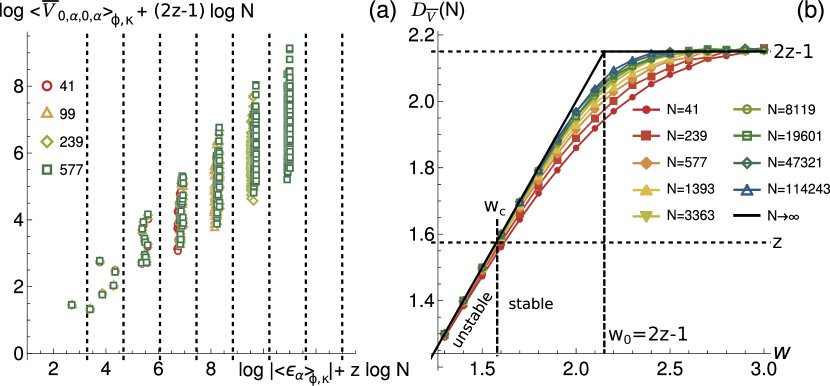
Figure 4: Scaling dimension of long range interactions. (a) Collapses of $\langle\bar{V}_{0\alpha 0\alpha}\rangle_{\phi,\kappa}$ calculated at the critical point of the half-filled Aubry-André model ($V=2$) for $\tau=1/\sqrt{2}$ (that has $z=1.575$), for different system sizes and different energies, and for power-law interactions with decay exponent $w=3$. Twisted boundary conditions are used and the results are averaged over $200$ random configurations of $\phi$ and $\kappa$, denoted by $\langle\rangle_{\phi,\kappa}$. (b) Finite-size results for $D_{\bar{V}}(N,w)$. The dashed lines indicate $D_{\bar{V}}=z$ and $D_{\bar{V}}=2z-1$. The black lines indicate the expected thermodynamic-limit behaviour. $w_{c}$ corresponds to the critical value of the exponent $w$ below which interactions become relevant.

Generalized Chalker scaling and irrelevance of generic short-range interactions.—

We now provide a framework to understand why the short range interactions we have studied so far are irrelevant. Our argument relies on a tree-level scaling analysis of the interaction at the critical point of the Aubry-André model. For completeness, we extend our discussion to long-range interactions, of the form $r^{-w}$ with $w>1$, and show there is a critical power law, $w_{c}$, where they eventually become relevant. We employ twisted boundary conditions and choose the long-range interaction to be a periodized form of the power-law potential $U\sum_{r,j}j^{-w}n_{r}n_{r+j}$, given by $U\sum_{j=1}^{N-1}N^{-w}\zeta(w,j/N)\sum_{r=1}^{N}n_{r}n_{r+j}$, where $\zeta(w,y)=\sum_{k=0}^{\infty}(k+y)^{-w}$ is the Hurwitz zeta function and $n_{r}=n_{r+N}^{\dagger}$ due to twisted boundary conditions. To compute the scaling dimension of the interaction term, denoted as $D_{U}(w)$, we write the interacting Hamiltonian on the single-particle eigenbasis of the non-interacting Aubry-André model Hamiltonian, $H_{0}$. We label single-particle states with Greek indices, ${\ket{\alpha}}$, and single-particle energies by $\epsilon_{\alpha}$. In this base

$$H=\sum_{\alpha}\epsilon_{\alpha}c^{\dagger}_{\alpha}c_{\alpha}-\sum_{\alpha,\beta,\gamma,\delta}\bar{V}_{\alpha\beta\gamma\delta}c^{\dagger}_{\alpha}c^{\dagger}_{\beta}c_{\gamma}c_{\delta}$$ (10)

where $\bar{V}_{\alpha\beta\gamma\delta}$ is the antisymmetrized version of the interaction tensor in the eigenbasis of the Aubry-André model

$$V_{\alpha\beta\gamma\delta}=\frac{U}{N^{w}}\sum_{r=1}^{N}\sum_{j=1}^{N-1}\zeta\Big{(}w,\frac{j}{N}\Big{)}\braket{\alpha}{r}\braket{\beta}{r+j}\braket{r}{\gamma}\braket{r+j}{\delta},$$ (11)

with $\braket{\alpha}{r}=\bra{0}c_{\alpha}c^{\dagger}_{r}\ket{0}$.

The leading contributions to the interacting term come from states with energies around the Fermi level, $E_{F}$. In the following, we denote by $\epsilon_{0}$ the energy closest to $E_{F}$ and we set $\epsilon_{0}=0$ for convenience. By the antisymmetry of $V$, the lowest-order non-vanishing contributions involve setting two indices to the Fermi level and varying the remaining, i.e. $\bar{V}_{\alpha 0\beta 0}$. Among those, we find that the dominant contribution arises for $\alpha=\beta$ (see SM) and thus we may restrict our analysis to an interaction tensor of the form $\bar{V}_{0\alpha 0\alpha}$ for small $|\epsilon_{\alpha}|$.

For the chosen model (half-filling, with $\tau=1/\sqrt{2}$), the critical point of the (non-interacting) Aubry-André model under a discrete scale transformation $r\to Nr$ is invariant under the rescaling $\epsilon_{\alpha}\rightarrow N^{z}\epsilon_{\alpha}$. The interacting term transforms as $\bar{V}_{0\alpha 0\alpha}\rightarrow N^{D_{\bar{V}}(w)}\bar{V}_{0\alpha 0\alpha}$, where $D_{\bar{V}}$ is the scaling dimension of the interaction tensor that can be obtained by the data collapse illustrated in Fig. 4(a). In this example, we take the half-filled Aubry-André model with $\tau=1/\sqrt{2}$, that has $z=1.575$, and set $w=3$, finding that $D_{\bar{V}}(w=3)=2z-1$. The relation between the energy, $\epsilon_{\alpha}$, and the interaction strength, $\bar{V}_{0\alpha 0\alpha}$, follows a generalized Chalker scaling (Chalker and Daniell, 1988; Chalker, 1990; Cuevas and Kravtsov, 2007; Foster et al., 2014; Chou et al., 2020). However, a significant difference to previous Chalker scaling analyses is the full antisymmetrization of the interaction term that follows from fermionic statistics.

By power-counting, we find the scaling dimension of the interaction to be $D_{U}=z-D_{\bar{V}}$, implying that interactions are irrelevant if $D_{\bar{V}}>z$ (see SM for details). To infere $D_{\bar{V}}(w)$ in the thermodynamic limit, we studied the finite-size dimension $D_{\bar{V}}(w,N_{m})$ (where $m$ labels the order of the approximant size $N_{m}$), which satisfies $D_{\bar{V}}(w,\infty)\equiv D_{\bar{V}}(w)$, and can be computed through $D_{\bar{V}}(w,N_{m})=-(\log N_{m+1}-\log N_{m})^{-1}[\log\bar{V}^{m+1}_{0101}(w)-\log\bar{V}^{m}_{0101}(w)]$, as depicted in Fig 4(b). As for the case $w=3$ shown in Fig 4(a), for sufficiently large $w>w_{0}=2z-1$, $D_{\bar{V}}=2z-1$. This scaling is also retrieved for other types of short-range interactions (e.g. finite range or exponentially suppressed), as we show in detail in the SM. Since $z>1$ at the critical point, interactions are always irrelevant in this case. This justifies the findings of previous sections near $U=U_{2}=0$. For $w<w_{0}$, the finite-size results shown in Fig 4(b) are compatible with $D_{\bar{V}}=w$. In this case, interactions become relevant for $w<z$ since at that point we start having $D_{\bar{V}}<z$ and thus $D_{U}>0$. The nature of this interesting fixed-point is left for future exploration.

Discussion.—

For a broad class of quasiperiodic models, we provided solid evidence that (i) short-range interactions are irrelevant at the LL-AG transition, not affecting the non-interacting critical exponents; (ii) a many-body generalization of the theory proposed in (Gonçalves et al., 2022b) can be formulated; and (iii) in the limit of vanishing interactions, the non-interacting critical point is robust to any short-range (and even some long-range) interactions. Our work not only provides a unified understanding of LL-AG transitions around criticality in terms of flows to non-interacting fixed-points accompanied by the emergence of many-body dualities in widely different models, but it also offers a very precise way to estimate the critical points. Future interesting questions to address include the effect of interactions on critical phases of the non-interacting quasiperiodic models, see e.g. the models in (Liu et al., 2015, 2022; Gonçalves et al., 2022c), and the nature of the fixed-point at which long-range interactions become relevant at the non-interacting Aubry-André critical point.

Supplemental Material for:

Short-range interactions are irrelevant at the quasiperiodic-driven Luttinger Liquid to Anderson Glass transition

S1 System size approximants used in finite-size simulations

In our finite-size simulations, we use rational approximants of $\tau$, $\tau_{c}=p/N$, with $p$ and $N$ co-prime numbers. These approximants were chosen to be exact convergents of the continued fraction expansion of $\tau$. This can be done as long as the unit cell defined by $\tau_{c}$ is equal to or larger than the system size, which guarantees that the system remains incommensurate. For our choice, the size of the unit cell is exactly the system size $N$. We chose the series of approximants given in table S1.

$N$	17	41	99	239	577	1393	$\infty$
$\tau_{c}$	$\frac{12}{17}$	$\frac{29}{41}$	$\frac{70}{99}$	$\frac{169}{239}$	$\frac{408}{577}$	$\frac{985}{1393}$	$\frac{1}{\sqrt{2}}$

.

Table S1: System size approximants of $\tau=1/\sqrt{2}$ used for the finite-size calculations.

S2 Additional scaling collapses: extracting $\nu$ and going away from half-filling

We start by extracting the critical exponent $\nu$ from the raw data on $\delta E_{\kappa\varphi}$, to validate our choice of $\nu=1$ in the main text. Assuming the ansatz $\delta E_{\kappa\varphi}\propto e^{-N/\xi}$ and that $\xi=gv^{-\nu}(N,\bm{\lambda})$, we have $\Lambda_{\kappa\varphi}=\log\delta E_{\kappa\varphi}=-Nv^{\nu}(N,\bm{\lambda})/g$ (note that $\delta E_{\kappa\varphi}=1$ for $v=0$) and therefore, we have $\log|\Lambda_{\kappa\varphi}|=\log N+\nu\log v-\log g$. We therefore carry out a linear multivariate fit using the data points $(\log N,\log|v|,\log|\Lambda_{\kappa\varphi}|)$ to extract $\nu$ and $\log g$. The results are in Fig. S1, where we show the fitting results as a function of the range $|\Delta v|$ below which data points were selected. The final results $\nu=1.001\pm 0.007$ and $g=0.972\pm 0.033$ were obtained by averaging the results (and fitting errors) for $\nu$ and $g$, for all the considered windows $\Delta v$.

For the non-interacting Aubry-André model, we have that $|\xi|=|1/\log(2t/V)|$ and therefore for $v\rightarrow 0$ we have $|\xi|=|v|^{-1}$ and $|\log\delta E_{\kappa\varphi}|=-N|v|$. This is consistent with the fitting results obtained for $\nu$ and $g$, which implies that close enough to the critical point, the correlation length behaves in the same way, irrespective of the considered model. Note that in principle, $g$ could depend on $\bm{\lambda}$ (the remaining parameters of the model), but we observed here for the studied models that close enough to criticality, $g\approx 1$.

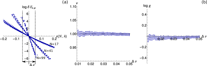
Figure S1: (a) Raw data used for fits to extract $\nu$. Each cluster of points corresponds to a different system size, indicated close to it. (b) Parameters extracted from a linear multivariate fit to the model $\log|\Lambda_{\kappa\varphi}|=\log N+\nu\log|v|-\log g$, by using data points $(\log N,\log v,\log|\Lambda_{\kappa\varphi}|)$ selected for different windows $\Delta v$ [represented in (a)].

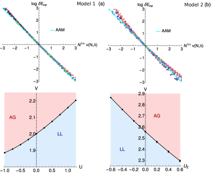
Figure S2: Results at filling $\rho=1/3$ for model 1 (a) and model 2 (b) defined in the main text. The bottom panels contain the phase transition points that we take to be $V_{c}(N=99,\bm{\lambda})$ (where $\bm{\lambda}$ contains the model parameters) with an error computed through $|V_{c}(99,\bm{\lambda})-V_{c}(41,\bm{\lambda})|$ (the difference in estimates for the largest used system sizes). Since the error is very small, $V_{c}(N=99,\bm{\lambda})$ already provides a very accurate estimation of $V_{c}(N=\infty,\bm{\lambda})$.

We finally show that the data collapse here observed is not a special feature of half-filling. For that purpose, we also obtain results for a filling $\rho=1/3$, again using models 1 and 2 defined in the main text. The results are in Fig. S2, showing nice collapses around criticality.

S3 Additional results for open boundary conditions

S3.1 Structure factor

We have seen in the main text that the Luttinger parameter $K$ approaches $1$ in the Luttinger liquid phase close to criticality, which implies that the small-$q$ behaviour of the static structure factor $S(q)$ is that of a non-interacting system. Here we explore in more detail the $S(q)$ behaviour at the critical point and in the localized phase. We will do so in the non-interacting (using the single-particle Hamiltonian) and interacting (using DMRG) cases. Let us derive an expression for $S(q)$ in the former case, using the single-particle eigenstates. In the non-interacting case, one can easily show that

$$S(q)=\frac{1}{N}\sum_{i,j=1}^{N}[(\Phi\Phi^{\dagger})_{ii}\delta_{ij}-(|\Phi\Phi^{\dagger}|^{2})_{ij}]e^{\textrm{i}q(i-j)}$$ (S1)

where $\Phi$ is a matrix containing the occupied single-particle eigenstates in its columns and $|.|^{2}$ squares all entries of matrix $\Phi\Phi^{\dagger}$.

In Fig. S3 we present results for the non-interacting Aubry-André model. We see that at small $q$, (i) $2\pi S(q)=Kq$ and $K\approx 1$ in the extended phase; (ii) $2\pi S(q)=Kq(1+a\sin[b+c\log(q)])$ and $K\approx 0.7$ at the critical point; (iii) $S(q)\sim q^{2}$ in the localized phase. Interestingly, at the critical point, there are clear $\log(q)$-periodic oscillations.

We now consider the family of interacting models given by Eq. 1 in the main text. The results for different choices of these interacting models are given in Fig. S4. There we see that in the LL phase we still have $S(q)\sim q$ [Figs. S4(a,b)]. However, we have that $2\pi S(q)=Kq$, with $K\neq 1$ sufficiently away from the critical point since the system becomes a truly interacting LL, as in the $V=0$ limit. As the critical point is approached, we have $K\rightarrow 1$. Exactly at the critical point, on the other hand, $S(q)$ shows an identical behaviour as in the non-interacting Aubry-André model’s critical point, see Fig. S4(c). It is remarkable to see that even though there are significant differences for larger $q$ for the different considered (interacting and non-interacting) critical points, the small-$q$ behaviour is the same. Interestingly, the amplitude of the log-periodic oscillations decreases in the interacting critical points, as can be seen in Fig. S4(d). Finally, in the AG phase we have $S(q)\sim q^{\eta}$ with $\eta\rightarrow 2$, compatible with the behaviour in the non-interacting localized phase, as shown in Figs. S4(b).

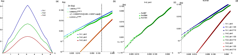
Figure S3: Results for non-interacting Aubry-André model, at half-filling [ $N_{p}=\lfloor\rho N\rfloor$, where $\lfloor x\rfloor$ takes the integer part of $x$ and $\rho=1/2$ ], using open boundary conditions. (a) Results for $V=1$ (extended phase), $V=2$ (critical point) and $V=3$ (localized phase). (b) Low $q$ behaviour of $S(q)$. The vertical dashed line denotes the largest $q$ considered for the fits to the expressions: (i) $2\pi S(q)=Kq^{\eta}$ in the extended phase, where we obtained $K,\eta\approx 1$ ; (ii) $2\pi S(q)=Kq^{\eta}(1+a\sin[b+c\log(q)])$ in the critical phase, where we extracted $K\approx 0.7$ and $\eta\approx 1$; (iii) $S(q)\sim q^{\eta}$ in the localized phase, where we extracted $\eta\approx 2$. Note that at the critical point, there are clear log-periodic oscillations. These are not a finite-size effect, as can be seen in (c), where different system sizes were considered and the oscillations are robust. (d) Dependence of $S(q)$ on $\phi$, for fixed $N=4181$. The results for different choices or $\phi$ are essentially the same, except at the critical point for small $q$, where there is a slight $\phi$-dependence, for fixed $N$.

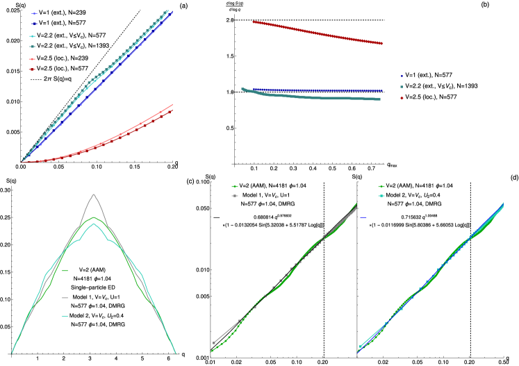
Figure S4: Results for interacting models, at half-filling, using open boundary conditions. (a) $S(q)$ for $U=1$ and $U_{2}=t_{2}=V_{2}=0,\phi=1.123$, for $V$ in the LL/extended phase ($V=1$), in the LL phase but close to the critical point ($V=2.2$) and in the AG phase ($V=2.5$). (b) Assuming that $S(q)\sim q^{\eta}$, we extract $\eta\equiv\partial\log S(q)/\partial\log q$ by making a linear fit to the $\log S(q)$ vs. $\log q$ data, from $q=0$ up to $q=q_{{\rm max}}$ (given in the x-axis of the figure). We see that in the LL phase, $\eta\approx 1$, while in the AG, $\eta\rightarrow 2$, as in the non-interacting case. (c) $S(q)$ at critical points obtained with significantly different parameters indicated in the figure, including the non-interacting case. We can see that in all cases, the small $q$ behaviour is very similar. (d) Log-log plot for the data in (c), along with fits to the expression $2\pi S(q)=Kq^{\eta}(1+a\sin[b+c\log(q)])$ for the interacting critical points, with the fit parameters given in the figure. Note that the vertical dashed line in the right panel denotes the largest $q$ considered for the fits. Neglecting the log-periodic oscillations, we get $2\pi S(q)=Kq$, with $K\approx 0.7$ in all cases.

S3.2 Natural orbitals

In the main text we have shown that the highest occupied natural orbitals are extended and localized, respectively at the LL and AG phases, and critical at the critical point. Here we show explicit plots, comparing the results with the density fluctuations $\delta n_{i}\equiv C^{ii}_{e}$. The results are in Fig. S5. We can see that when the critical point is approached from the LL phase, $\delta n_{i}$ becomes very close to $|\psi_{i}^{(0)}|^{2}$, signaling the irrelevance of interactions (in the non-interacting case, these quantities are equal).

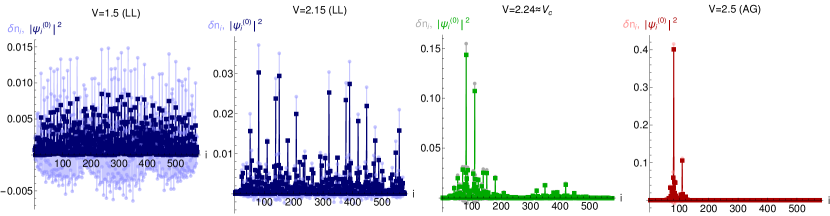
Figure S5: Plots of the squared amplitudes of natural orbitals, $|\psi_{i}^{(0)}|^{2}$, and of the density fluctuations $\delta n_{i}$ for $N=577$, with $U=1$ and $U_{2}=t_{2}=V_{2}=0$, and $\phi=1.123$, for different $V$.

To finish this section and complement multifractal analysis carried out in Fig. 3(b) of the main text, we show explicit data for $\langle\textrm{IPR}_{N0}(q=2)\rangle_{\phi}$ as a function of system size $N$, from which the exponent $\tau(q=2)$ was extracted. The results are shown in Fig. S6.

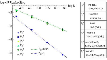
Figure S6: $\langle\textrm{IPR}_{N0}(q=2)\rangle_{\phi}$ for different models with chosen parameters indicated in the table at right, where $P_{i}^{e}$($P_{i}^{c}$) denote extended (critical) points. In the table, $V_{c}$ corresponds to the estimated critical point. $\langle\rangle_{\phi}$ denotes an average over different choices of $\phi$. We took $\phi_{j}=2\pi j/N_{c},\textrm{ }j=0,\cdots,N_{c}-1$ and $N_{c}\in[100-300]$. The blue and green dashed lines in (c) shows the scaling behaviour in the non-interacting Aubry-André model, respectively at extended and critical points.

S3.3 Entanglement entropy

In the main text, we mentioned that the entanglement entropy, $\mathcal{S}$, shows showing log-periodic oscillations as a function of the subsystem size, at the critical point of the non-interacting Aubry-André model. In Fig. S7(a) we show the numerical results supporting this claim in a log-linear plot. By averaging $\mathcal{S}$ over a sufficiently large number of $\phi$-configurations, we see that these oscillations are robust to increasing the system size. In Fig. S7(b) we also show that these oscillations persist in the presence of interactions, at the critical point.

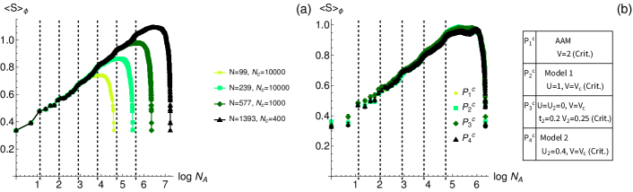
Figure S7: (a) Entanglement entropy $\mathcal{S}$ as a function of the size of sub-system $A$, consisting of the first $N_{A}$ sites, for the non-interacting Aubry-André model. We used different system sizes and averaged over $N_{c}$ configurations of $\phi$ given by $\phi_{j}=2\pi j/N_{c},\textrm{ },j=0,\cdots,N_{c}-1$. The vertical dashed lines are guides to the eye, showing the log-periodic maxima of the oscillations. (b) DMRG results at different critical points obtained for the parameter choices given in the table, averaging over $N_{c}\in[100-300]$ configurations.

S4 Duality transformation

Here we build a many-body generalization of the duality transformation introduced in Ref. (Gonçalves et al., 2022a). We start by writing the most occupied natural orbital as $\ket{\alpha=0}=\sum_{i}\psi_{i}^{(0)}\ket{i}$, and defining its Fourier transform as

$$\tilde{\psi}_{k}^{(0),d}=\frac{1}{\sqrt{N}}\sum_{i=0}^{N-1}e^{\textrm{i}2\pi\tau_{c}ki}\psi_{i}^{(0)}.$$ (S2)

The hidden duality transformations defined in Ref. (Gonçalves et al., 2022a) map points $(\phi,k)=(\phi_{0}+\Delta\phi,k_{0}+\Delta k)$ to points $(\phi^{\prime},k^{\prime})=(\phi_{0}+\Delta k,k_{0}+\Delta\phi)$, where $(\phi_{0},k_{0})$ is the “center” of the hidden duality transformation. Setting $(\phi_{0},k_{0})=(\varphi_{0},\kappa_{0})$, with $(\varphi_{0},\kappa_{0})$ given in the main text for the different used system sizes yields a possible choice for which $\bm{\psi}^{(0)}\propto\tilde{\bm{\psi}}^{(0),d}$ at the self-dual point of the non-interacting Aubry-André model ($V=2$). For more generic choices, we would need to compute $\psi_{i}^{(0)}$ at $(\phi,k)=(\phi_{0}+\Delta\phi,k_{0}+\Delta k)$ and $\tilde{\psi}_{k}^{(0),d}$ at $(\phi^{\prime},k^{\prime})=(\phi_{0}+\Delta k,k_{0}+\Delta\phi)$ to have $\bm{\psi}^{(0)}\propto\tilde{\bm{\psi}}^{(0),d}$.

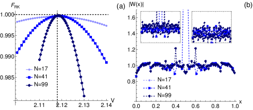
Figure S8: (a) $F_{RK}$ defined in the text for $U=0.5$ and $U_{2}=V_{2}=t_{2}=0$. The dashed black line indicates $V=V_{c}(N=99)$. (b) Duality function $\chi(x)$ introduced in Ref. (Gonçalves et al., 2022b) defined through the natural orbital at $V=V_{c}(N)$. The insets show the results if $\chi(x)$ was computed at the points marked in (a), slightly away from the critical point: in this case we obtain a featureless function, not robust to increasing $N$.

In Fig. S8(a) we computed $F_{RK}\equiv(\tilde{\bm{\psi}}^{(0),d})^{*}\cdot\bm{\psi}^{(0)}$ using $(\phi,k)=(\phi_{0},k_{0})=(\varphi_{0},\kappa_{0})$ for model 1 with $U=0.5$ as an example. We see that $F_{RK}$ decreases with $N$, except when we cross the critical point, where it becomes very close to $1$. This suggests that $\bm{\psi}^{(0)}$ is almost equal to $\tilde{\bm{\psi}}^{(0),d}$ at this point. We can go one step further and define the duality transformation that relates $\bm{\psi}^{(0)}$ and $\tilde{\bm{\psi}}^{(0),d}$ at self-dual points as in Ref. (Gonçalves et al., 2022b) (where the natural orbital replaces the role of the single-particle wave function).

From $\bm{\psi}^{(0)}$ and $\bm{\tilde{\psi}}^{(0),d}$, we then define the duality matrix $\mathcal{O}_{c}$ as in Ref. (Gonçalves et al., 2022a):

$$\mathcal{O}_{c}[T^{n}\bm{\tilde{\psi}}^{(0),d}]=T^{n}\bm{\psi}_{i}^{(0)},\hskip 10.00002ptn=0,\cdots,L-1,$$ (S3)

where $T$ is the cyclic translation operator defined as $T\psi=\psi^{\prime}$ with $\psi^{\prime}_{i}=\psi_{\mod(i+1,L)}$. Since $\mathcal{O}_{c}$ is a circulant matrix, we may write it as

$$\mathcal{O}_{c}=U^{\dagger}WU$$ (S4)

where $U$ is a matrix with entries $U_{ij}=e^{2\pi{\rm i}\tau_{c}ij}$ and $W$ is a diagonal matrix $W_{ij}=w_{j}\delta_{ij}$ with the eigenvalues $\{w_{j}\}$ of $\mathcal{O}_{c}$. We can therefore write

$$\bm{\psi}^{(0)}=U^{\dagger}W\bm{\psi}^{(0)}\leftrightarrow\psi_{i}^{(0)}=\sum_{\nu=0}^{L-1}e^{2\pi i\tau_{c}ij}w{}_{j}\psi_{j}^{(0)}.$$ (S5)

The eigenvalues $w_{j}$ are, as seen in Ref. (Gonçalves et al., 2022a), evaluations of a function $W(x)$, that has period $\Delta x=1$, at points $x_{j}=\mod\Big{(}j\tau_{c}+\frac{\phi}{2\pi},1\Big{)},\textrm{ }j=0,\cdots,L-1$. This function is sampled in the whole interval $x\in[0,1[$ in the limit that $\tau_{c}\rightarrow\tau$ ($N\rightarrow\infty$) and encodes all the information on the duality transformation $W$. We show an example of the duality function $W(x)$ in Fig. S8(b), where we see that a complicated function with features that are robust to the increasing of $N$ is formed. $W(x_{j})$ only has the meaning of a duality transformation if $\bm{\psi}^{(0)}$ and $\tilde{\bm{\psi}}^{(0),d}$ are computed at self-dual points (or at dual points in the extended and localized phases, a case that was not considered here). We can however compute $W(x_{j})$ in the same way by using $\bm{\psi}^{(0)}$ and $\tilde{\bm{\psi}}^{(0),d}$ at any point, but in this case, since there is no duality transformation connecting the wave functions, we expect $W(x_{j})$ to be featureless and not robust for increasing system size. This is clearly shown in the insets of Fig. S8(b).

S5 Generalized Chalker scaling and irrelevance of generic short-range interactions

We show that generic short-range (and some long-range) interactions are irrelevant at the critical point of the Aubry-André model in the $U\rightarrow 0$ limit, by unveiling the existence of a generalized Chalker scaling (Chalker and Daniell, 1988; Chalker, 1990; Cuevas and Kravtsov, 2007; Foster et al., 2014; Chou et al., 2020) at this point. All the results that we present in this section are for the parameters studied in the main text, namely $\tau=1/\sqrt{2}$ and at half-filling, with $N_{p}=\lfloor N/2\rfloor$ particles. Nonetheless, the technology here developed can be (and was) applied to more generic cases, as we comment at the end of the section.

We consider the periodized form of the power-law interactions $U\sum_{j}j^{-w}n_{r}n_{r+j}$, given by

$$U\sum_{j=1}^{N-1}\sum_{k=0}^{\infty}(j+kN)^{-w}\sum_{r}n_{r}n_{r+j+kN}=U\sum_{j=1}^{N-1}N^{-w}\zeta(w,j/N)\sum_{r=1}^{N}n_{r}n_{r+j},$$ (S6)

where $\zeta(w,y)=\sum_{k=0}^{\infty}(k+y)^{-w}$ is the Hurwitz zeta function and $c_{r}^{\dagger}=c_{r+kN}^{\dagger},k\in\mathbb{Z}$ due to periodic boundary conditions. For such interaction, we can write the path integral for the grassman variables $\bar{c},c$ as

$$Z=\int\mathcal{D}[\bar{c},c]e^{-(S_{0}[\bar{c},c]+S_{U}[\bar{c},c])}$$ (S7)

where, writing in the single-particle eigenbasis of the non-interacting Aubry-André model Hamiltonian $H_{0}$ (Eq. 1, with $t_{2}=V_{2}=U=U_{2}=0$) with eigenenergies $\epsilon_{\alpha}=E_{\alpha}-\mu$ (measured relative to the chemical potential $\mu$), we have

$$S_{0}=\int_{0}^{\infty}d\tau\sum_{\alpha}\bar{c}_{\alpha}(\tau)(\partial_{\tau}+\epsilon_{\alpha})c_{\alpha}(\tau)$$ (S8)

$$S_{U}=-U\int_{0}^{\infty}d\tau\sum_{\alpha,\beta,\gamma,\delta}\bar{V}_{\alpha\beta\gamma\delta}\bar{c}_{\alpha}(\tau)\bar{c}_{\beta}(\tau)c_{\gamma}(\tau)c_{\delta}(\tau)$$ (S9)

and where $\bar{V}_{\alpha\beta\gamma\delta}=\Big{(}V_{\alpha\beta\gamma\delta}-V_{\beta\alpha\gamma\delta}+V_{\beta\alpha\delta\gamma}-V_{\alpha\beta\delta\gamma}\Big{)}/4$ is the antisymmetrized version of the interaction matrix elements

$$V_{\alpha\beta\gamma\delta}=\sum_{r=1}^{N}\sum_{j=1}^{N-1}N^{-w}\zeta(w,j/N)\braket{\alpha}{r}\braket{\beta}{r+j}\braket{r}{\gamma}\braket{r+j}{\delta}$$ (S10)

We will now inspect the interacting part in detail. We have a 4-leg tensor on our hands. We want to study this tensor close to $\alpha,\beta,\gamma,\delta=0$, where 0 denotes the Fermi level. Since the tensor is antisymmetric, $\bar{V}_{0000}=0$. We can now inspect different combinations of indices to see how the 4-leg tensor behaves as the indices depart from 0. We can start by fixing 3 of the indices to be 0 and varying the remaining index. However, this yields zero due to antisymetry. We can also now fix 2 indices to 0 and vary the remaining 2 indices that we call $\alpha$ and $\beta$. The possible contributions are $\bar{V}_{0\alpha 0\beta}$, $\bar{V}_{\alpha 0\beta 0}$=$\bar{V}_{0\alpha 0\beta}$, $\bar{V}_{00\alpha\beta}=\bar{V}_{\alpha\beta 00}=0$ and $\bar{V}_{\alpha 00\beta}=\bar{V}_{0\alpha\beta 0}=-\bar{V}_{0\alpha 0\beta}$. Therefore, the only contribution that we need to compute is $\bar{V}_{0\alpha 0\beta}$, as all the others are either zero or can be obtained from this one. In Fig. S9 we show that the most important contribution arises for $\alpha=\beta$ (we show examples for $w=1.5$ and $w=3$, but this remains true for other values of $w$). Therefore, we will focus on the contribution $\bar{V}_{0\alpha 0\alpha}$. Note that higher-order contributions involve setting only one index to 0 and varying the others, but is already a contribution involving 3 energies, that we assume to be neglegible as $\alpha,\beta,\gamma,\delta\rightarrow 0$. We then write the interacting part of the action as

$$S_{U}=-4U\int_{0}^{\infty}d\tau\sum_{\alpha}\bar{V}_{0\alpha 0\alpha}\bar{c}_{0}(\tau)\bar{c}_{\alpha}(\tau)c_{0}(\tau)c_{\alpha}(\tau)+\mathcal{O}(\epsilon_{\alpha}^{\mu}\epsilon_{\gamma}^{x})$$ (S11)

where we assumed that $\bar{V}_{0\alpha 0\alpha}\sim\epsilon_{\alpha}^{\mu}$ and $\gamma$ denotes the additional index (or indices) that we choose to make finite in tensor $\bar{V}_{0\alpha 0\alpha}$ [for instance $\bar{V}_{0\alpha\gamma\alpha}=\bar{V}_{0\alpha 0\alpha}+\mathcal{O}(\epsilon_{\alpha}^{\mu}\epsilon_{\gamma}^{x})$] and the exponent $x$ may depend on this choice of indices. This contribution will therefore either be neglegible or the same as of $\bar{V}_{0\alpha 0\alpha}$, if $x=0$. The term $\bar{V}_{0\alpha 0\alpha}$ can be written explicitly as

$$\begin{array}[]{cc}\bar{V}_{0\alpha 0\alpha}=&\frac{1}{4}\sum_{j=1}^{N-1}N^{-w}\zeta(q,j/N)\Bigg{(}\sum_{r=1}^{N}(|\braket{0}{r}|^{2}|\braket{\alpha}{r+j}|^{2}+|\braket{\alpha}{r}|^{2}|\braket{0}{r+j}|^{2})\\ &-\sum_{r=1}^{N}\braket{0}{r}\braket{r}{\alpha}\braket{\alpha}{r+j}\braket{r+j}{0}-\sum_{r=1}^{N}\braket{\alpha}{r}\braket{r}{0}\braket{0}{r+j}\braket{r+j}{\alpha}\Bigg{)}\end{array}$$ (S12)

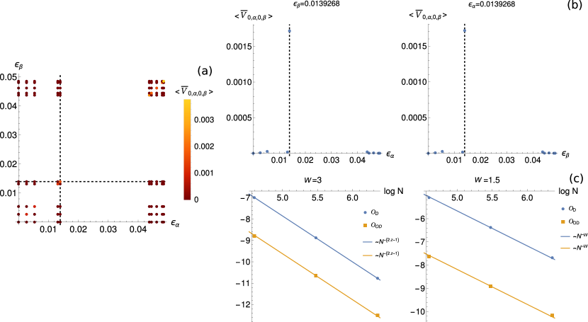
Figure S9: (a) $\langle\bar{V}_{0\alpha 0\beta}\rangle_{\phi,\kappa}$ for $N=239$, $w=1.5$ and $\alpha,\beta=0,\cdots,9$, averaged over $200$ random configurations of $\phi$ and $\kappa$. We can see that the dominant contribution occurs for $\alpha=\beta$. This can also be seen in (b), where we make the cuts marked in (a) by the dashed lines. The vertical dashed line in (b) indicates the diagonal contribution, which is much larger than the remaining ones. In (c) we show that this conclusion is robust to increasing $N$. To do so, we compute the average diagonal, $\mathcal{O}_{\textrm{OD}}=\frac{1}{n^{2}-n}\sum_{\alpha\neq\beta}^{n}\langle\bar{V}_{0\alpha 0\beta}\rangle_{\phi,\kappa}$, and off-diagonal, $\mathcal{O}_{\textrm{D}}=\frac{1}{n}\sum_{\alpha=1}^{n}\langle\bar{V}_{0\alpha 0\alpha}\rangle_{\phi,\kappa}$, contributions (fixing $n=9$, independently of $N$). Results are shown for $w=3$ (left) and $w=1.5$ (right) as examples. $\mathcal{O}_{\textrm{OD}}$ and $\mathcal{O}_{\textrm{D}}$ scale identically with $N$, implying that the diagonal contribution dominates for any $N$.

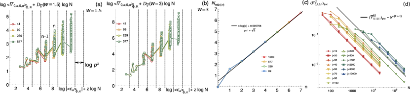
Figure S10: (a,b) $\langle\bar{V}_{0\alpha 0\alpha}\rangle_{\phi,\kappa}$ averaged over 200 random configurations of $\phi$ and $\kappa$ ($\langle\rangle_{\phi,\kappa}$ denotes the average over $\phi,\kappa$ configurations) for $w=1.5$ (a) and $w=3$ (b), where $D_{\bar{V}}(w=1.5)=w$ and $D_{\bar{V}}(w=3)=2z-1$, with $z=1.575$ being the dynamical critical exponent. (c) Number of states in each miniband, $N_{{\rm mb}(n)}$. Note that the minibands are only well-defined (that is, there are clear clusters of states) for $n\geq 2$, above which the scaling $N_{{\rm mb}(n)}\propto p^{n}$ is observed. The dashed lines in (a,b) are separated by $\log p^{z}$, implying that the average energy of each miniband scales as $p^{zn}$. (d) $\langle\bar{V}^{(j)}_{0\alpha 0\alpha}\rangle_{\phi,\kappa}$ for the interaction term in Eq S20, and for $\alpha=1$, as a function of system size $N$ and averaged over 4800 random configurations of $\phi$ and $\kappa$.

In Figs. S10(a,b), we show that it is possible to collapse the results for $\bar{V}_{0\alpha 0\alpha}$ for different approximant system sizes and different energies. The collapse becomes better as $\epsilon_{\alpha}\rightarrow 0$. Furthermore, there are clusters of eigenvalues that form on the $\log|\epsilon_{\alpha}|$ scale, that we will can “minibands” in the following. In Fig. S10(c) we can see that the number of states in each miniband scales as $N_{{\rm mb}(n)}\propto p^{n}$. By realizing that increasing the order of system size approximant introduces a new miniband, we can easily find that $p=N_{m+1}/N_{m}\rightarrow 1+\sqrt{2}$ as $m\rightarrow\infty$ where $N_{m}$ is the m-th order system size approximant for $\tau=1/\sqrt{2}$. By defining $\bar{\epsilon}_{n}^{(m)}=N_{{\rm mb}(n)}^{-1}\sum_{\alpha\in{\rm mb(n)}}\epsilon_{\alpha}^{(m)}$ (where the superscript “(m)” indicates the eigenenergies for the m-th order size approximant), we also have that $\bar{\epsilon}_{n}\propto p^{nz}$, as indicated in Fig. S10(a), where $z=1.575$ is the dynamical critical exponent. Naturally, the scaling collapse in this figure also implies that $\epsilon_{\alpha}^{(m-l)}=p^{zl}\epsilon_{\alpha}^{(m)}$. These observations allow us to write the following ansatz,

$$\bar{V}_{0\alpha 0\alpha}=\mathcal{C}N_{m}^{-D_{\bar{V}}}(|\epsilon_{\alpha}^{(m)}|N_{m}^{z})^{\mu}\sum_{n}f([|\epsilon_{\alpha}^{(m)}|-\bar{\epsilon}_{n}^{(m)}]N_{m}^{z})$$ (S13)

where $\mathcal{C}$ is some constant independent of energy and $N_{m}$. We note that, as shown in Figs. S10(a,b) and in the main text, $D_{\bar{V}}$ depends on $w$. We will discuss this dependence below in more detail below. At this point we also note that when averaged over minibands, $\bar{V}_{0\alpha 0\alpha}\sim(|\epsilon_{\alpha}^{(m)}|)^{\mu}$, where $\mu>0$. This shows that there is a generalized Chalker scaling (Chalker and Daniell, 1988; Chalker, 1990; Cuevas and Kravtsov, 2007; Foster et al., 2014; Chou et al., 2020) at the critical point of the Aubry-André model, manifested by power-law correlations (on average) between the single-particle eigenfunctions with respect to their energy difference.

To carry out a power-counting analysis and inspect the scaling dimension of the interactions, we take a large enough system size to begin with so that the data collapse is quite good for the relevant energies of choice and Eq. S13 holds. In each renormalization-group (RG) step, we throw away a miniband and rescale the energies. Starting with an energy cutoff $\Lambda_{k}$, after $l$ RG steps we end up with a cutoff $\Lambda_{k+l}=\Lambda_{k}/p^{zl}$. We also start with an initial system size $N_{m}$. The non-interacting action $S_{0}$, after introducing the cutoff, is given by

$$S_{0}^{\Lambda_{k},N_{m}}=\int_{0}^{\infty}d\tau\int_{-\Lambda_{k}}^{\Lambda_{k}}d\epsilon\textrm{ }\sum_{\alpha}\delta(\epsilon-\epsilon_{\alpha}^{(m)})\bar{c}(\epsilon,\tau)(\partial_{\tau}+\epsilon)c(\epsilon,\tau)$$ (S14)

After after $l$ RG steps, it becomes:

$$S_{0}^{\Lambda_{k+l},N_{m}}=\int_{0}^{\infty}d\tau^{\prime}\int_{-\Lambda_{k}}^{\Lambda_{k}}d\epsilon^{\prime}\textrm{ }\sum_{\alpha}\delta(\epsilon^{\prime}-\epsilon_{\alpha}^{(m-l)})\bar{c}(\epsilon^{\prime},\tau^{\prime})\Big{(}\partial_{\tau^{\prime}}+\epsilon^{\prime}\Big{)}c(\epsilon^{\prime},\tau^{\prime})=S_{0}^{\Lambda_{k},N_{m-l}}$$ (S15)

where we used $\epsilon^{\prime}=p^{zl}\epsilon\textrm{ , $\tau^{\prime}=\tau p^{-zl}$},\epsilon_{\alpha}^{(m-l)}=p^{zl}\epsilon_{\alpha}^{(m)}$ and defined $\bar{c}(\epsilon^{\prime}p^{-zl},\tau^{\prime}p^{zl})=\bar{c}(\epsilon^{\prime},\tau^{\prime});\textrm{ }c(\epsilon^{\prime}p^{-zl},\tau^{\prime}p^{zl})=c(\epsilon^{\prime},\tau^{\prime})$. The new action after $l$ RG steps therefore corresponds to the same action, but for a smaller system size $N_{m-l}$. For the interacting part, we have

$$S_{U}^{\Lambda_{k},N_{m}}=-U\mathcal{C}N_{m}^{-D_{\bar{V}}}\sum_{\alpha}\int_{-\Lambda_{k}}^{\Lambda_{k}}d\epsilon\delta(\epsilon-\epsilon_{\alpha}^{(m)})(|\epsilon|N_{m}^{z})^{\mu}\sum_{n}f([|\epsilon|-\bar{\epsilon}_{n}^{(m)}]N_{m}^{z})\bar{c}(0,\tau)\bar{c}(\epsilon,\tau)c(0,\tau)c(\epsilon,\tau)$$ (S16)

where the factor 4 in Eq S11 was absorved in the constant $\mathcal{C}$. The full action for the interacting part after $l$ RG steps is therefore

$$\begin{array}[]{cc}S_{U}^{\Lambda_{k+l},N_{m}}=-U\mathcal{C}p^{-(D_{\bar{V}}-z)l}N_{m-l}^{-(D_{\bar{V}}-z)}\int d\tau^{\prime}\sum_{\alpha}\int_{-\Lambda_{k}}^{\Lambda_{k}}d\epsilon^{\prime}\textrm{ }\delta(\epsilon^{\prime}-\epsilon_{\alpha}^{(m-l)})(|\epsilon^{\prime}|N_{m-l}^{z})^{\mu}\\ \times\sum_{n}f([|\epsilon^{\prime}|-\bar{\epsilon}_{n}^{(m-l)}]N_{m-l}^{z})\bar{c}(0,\tau^{\prime})\bar{c}(\epsilon^{\prime},\tau^{\prime})c(0,\tau^{\prime})c(\epsilon^{\prime},\tau^{\prime})\\ =p^{-(D_{\bar{V}}-z)l}S_{U}^{\Lambda_{k},N_{m-l}}\end{array}$$ (S17)

In summary, after $l$ RG steps we have:

$$S^{\Lambda_{k+l},N_{m}}=S_{0}^{\Lambda_{k+l},N_{m}}+S_{U}^{\Lambda_{k+l},N_{m}}=S_{0}^{\Lambda_{k},N_{m-l}}+p^{-(D_{\bar{V}}-z)l}S_{U}^{\Lambda_{k},N_{m-l}}$$ (S18)

This implies that interactions the scaling dimension of the interacting part is $z-D_{\bar{V}}$, and therefore interactions are irrelevant when $D_{U}=D_{\bar{V}}>z$. In Fig 4(b) of the main text, we have seen that the thermodynamic-limit behaviour of $D_{\bar{V}}(w)$ is compatible with

$$D_{\bar{V}}(w)=\begin{cases}w&,w<2z-1\\ 2z-1&,w\geq 2z-1\end{cases}$$ (S19)

This implies that interactions are irrelevant for $w>z$, marginal for $w=z$ and relevant for $w<z$. The relevance of interactions for $w<z$ is left for future exploration. These results also imply that even when long-range interactions are considered, they can be irrelevant in the $U\rightarrow 0$ limit if they decay fast enough. On the other hand, it also follows that short-range interactions have $D_{\bar{V}}=2z-1$ and therefore their scaling dimension is $D_{U}=1-z$. Since $z>1$ at the critical point, short-range interactions are irrelevant. At the extended phase, on the other hand, $z=1$, which implies that interactions are marginal, in agreement with the $V=0$ results.

To show that short-range interactions are irrelevant in more detail, we consider the following finite-range interacting terms (again assuming periodic boundary conditions),

$$H_{U}^{(j)}=U\sum_{r=1}^{N}n_{r}n_{r+j}$$ (S20)

and compute the associated antisymmetrized interaction $\bar{V}^{(j)}_{0101}\propto N^{-D_{\bar{V}}}$ for each interaction term of this type, in Fig. S10(d). We find that no matter the interaction range $j$, if the system size becomes sufficiently larger than this range $D_{\bar{V}}(N)\rightarrow 2z-1$. Therefore, any short-range function of these interaction terms should also follow this behaviour. With this in mind, we expect that the universal behaviour unveiled in this work is not restricted to the interactions studied in Eq 1, but also holds for more generic short-range (and even some long-range) interactions. Even though in this section we focused on the choices of parameters used in the main text, we checked that the same conclusions can also be drawn for other fillings and other values of $\tau$ also considered in (Cookmeyer et al., 2020).

We finish this section by showing that the short-range dimension $D_{\bar{V}}=2z-1$ can be understood from simple arguments. We start by writing

$$\bar{V}_{0101}=N^{-D_{\bar{V}}}f(\epsilon_{g}N^{z})$$ (S21)

assuming that $D_{\bar{V}}$ is unknown, where $\epsilon_{g}$ is the energy gap for a system size $N$. Since we have $\epsilon_{g}=KN^{-z}$, where $K$ is a constant, we know that $\bar{V}_{0101}=N^{-D_{\bar{V}}}f(K)\sim N^{-D_{\bar{V}}}$ and therefore

$$\bar{V}_{0101}=\epsilon_{g}^{D_{\bar{V}}/z}$$ (S22)

On the other hand, we can write

$$\bar{V}_{0101}=\sum_{r=1}^{N}\bar{V}_{\epsilon_{g}}^{r}$$ (S23)

where

$$\bar{V}_{\epsilon_{g}}^{r}=\frac{1}{4}\Bigg{(}|\braket{0}{r}|^{2}|\braket{1}{r+j}|^{2}+|\braket{1}{r}|^{2}|\braket{0}{r+j}|^{2}$$ (S24)

$$-(\braket{0}{r}\braket{r}{1}\braket{1}{r+j}\braket{r+j}{0}+\textrm{c.c})\Bigg{)}$$

After averaging over $\phi$ and $\kappa$, translational invariance is restored and $\bar{V}_{\epsilon}^{r}$ becomes r-independent. Furthermore, we know that $\bar{V}_{\epsilon_{g}}^{r}\rightarrow 0$ as $\epsilon_{g}\rightarrow 0$. Expanding $\bar{V}_{\epsilon_{g}}^{r}$ in powers of $\epsilon_{g}$, assuming it to be a regular function:

$$\bar{V}_{\epsilon_{g}}^{r}=a_{1}\epsilon_{g}+a_{2}\epsilon_{g}^{2}+\cdots$$ (S25)

We have that $a_{1}=0$ since it can be easily shown that $\bar{V}_{\epsilon_{g}}^{r}\geq 0$ for any $\epsilon_{g}$. We therefore have

$$\bar{V}_{0101}\sim N\epsilon_{g}^{2}\sim\epsilon_{g}^{2-1/z}$$ (S26)

By comparing with Eq. S22, this therefore implies that $D_{\bar{V}}=2z-1$. Therefore, we conclude that the scaling dimension for short-range interactions simply follows from $\bar{V}_{\epsilon_{g}}^{r}$ being a regular function of $\epsilon_{g}$.

S6 Charge gap scaling for alternative choices of $\tau$ and filling $\rho$

From the results that we obtained in the main text, we have seen that the scalings of the charge gap (and other quantities such as the fractal dimension) with system size obtained at different LL-AG transitions are compatible, no matter the chosen parameters (hoppings, potential, interactions), at half-filling ($\rho=1/2$) and for approximants of $\tau=1/\sqrt{2}$ [Fig. 3 of the main text]. A natural question that arises is whether this is a special feature of our choice of $\rho$ and $\tau$. In particular, we know that the dynamical exponent $z$ depends on both $\rho$ and $\tau$ in the non-interacting limit, for the Aubry-André model Cookmeyer et al. (2020). If we make other choices of $\rho$ and $\tau$, is the charge gap scaling also independent on the remaining Hamiltonian parameters, as long as we are at the critical point? Since this is a question that we can already ask in the non-interacting limit, we will take the class of models considered in the main text, in the non-interacting limit, with Hamiltonian given by:

$$\begin{aligned} H=&-\sum_{i}c_{i}^{\dagger}c_{i+1}+t_{2}\sum_{i}c_{i}^{\dagger}c_{i+2}+{\rm h.c.}\\ &+\sum_{i}\Big{(}V\cos(2\pi\tau_{c}i+\phi)+V_{2}\cos[2(2\pi\tau_{c}i+\phi)]\Big{)}c_{i}^{\dagger}c_{i}\end{aligned}\textrm{ GAA model}$$ (S27)

For the finite-size scaling results that follow, we use open boundary conditions and the sizes and rational approximants $\tau_{c}$ given in table S2. The results are given in Fig. S11, where we can see that the scalings obtained at critical points of widely different models are very compatible for fixed $\rho$ and $\tau$. In some cases, there are more than one scaling functions, which means that an accurate finite-size scaling analysis should consider the system sizes that belong to the different scaling functions separately Cookmeyer et al. (2020). Remarkably, even the scaling features that arise due to the existence of multiple scaling functions (e.g., the 3-step scaling in Fig. S11 due to the existence of 3 scaling functions) holds at different critical points as long as $\rho$ and $\tau$ are fixed. These results support our claim that the scaling invariance that we observed at the critical point is not a special feature of our choice of $\rho$ and $\tau$. We checked for additional models, e.g. the model in Ref. Ganeshan et al. (2015), and obtained compatible results.

$\tau=1/\sqrt{2}$
$N$	41	99	239	577	1393	3363
$\tau_{c}$	$\frac{29}{41}$	$\frac{70}{99}$	$\frac{169}{239}$	$\frac{408}{577}$	$\frac{985}{1393}$	$\frac{2378}{3363}$
$N_{c}$	500	500	500	500	500	300

$\tau=(\sqrt{5}-1)/2$
$N$	34	55	89	144	233	377	610	987	1597	2584	4181
$\tau_{c}$	$\frac{21}{34}$	$\frac{34}{55}$	$\frac{55}{89}$	$\frac{89}{144}$	$\frac{144}{233}$	$\frac{233}{377}$	$\frac{377}{610}$	$\frac{610}{987}$	$\frac{987}{1597}$	$\frac{1597}{2584}$	$\frac{2584}{4181}$
$N_{c}$	1000	1000	1000	1000	750	750	500	500	500	300	250

Table S2: Choices of sizes $N$, rational approximants $\tau_{c}$ and number of $\phi$-configurations $N_{c}$ for $\tau=1/\sqrt{2}$ and $\tau=(\sqrt{5}-1)/2$. The different phases $\phi$ were chosen from a uniform grid given by $\phi_{j}=2\pi j/N_{c},j=0,\cdots,N_{c}-1$.

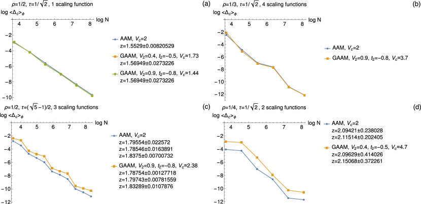
Figure S11: Scaling of the charge gap using open boundary conditions and averaged over $\phi$, for different fillings and choices of $\tau$ and at critical points of different models. The different critical points were estimated by imposing twisted boundary conditions and estimating the value $V=V_{c}$ for which $\Delta E_{\kappa\varphi}=1$ (leaving the remaining parameters fixed), for the largest used system size. We indicate all the relevant parameters in the figure and also the number of scaling functions for the selected $\tau$ and $\rho$, that were obtained in Cookmeyer et al. (2020). The values of $z$ indicated are extracted from fits using sizes $N_{\mathcal{N}j+1},j=0,\cdots,j_{{\rm max}}$ of the lists given in table S2, where $\mathcal{N}$ is the number of scaling functions. In (a) we used the $5$ largest sizes, in (c) the 3 largest sizes belonging to each scaling function and in (d) we used all sizes. The different $z$ estimates in (c,d) for the same critical points were obtained from fits to sizes that belong to the different existing scaling functions.