Model-agnostic cosmological constraints from the baryon acoustic oscillation feature in redshift space

Abstract

We develop a framework for self-consistently extracting cosmological information from the clustering of tracers in redshift space, without relying on model-dependent templates to describe the baryon acoustic oscillation (BAO) feature. Our approach uses the recently proposed Laguerre reconstruction technique for the BAO feature and its linear point $r_{\rm LP}$, and substantially extends it to simultaneously model the multipoles $\ell=0,2,4$ of the anisotropic galaxy 2-point correlation function (2pcf). The approach is ‘model-agnostic’: it assumes that the non-linear growth of structure smears the BAO feature by an approximately Gaussian kernel with a smearing scale $\sigma_{\rm v}$, but does not assume any fiducial cosmology for describing the shape of the feature itself. Using mock observations for two realistic survey configurations assuming $\Lambda$ cold dark matter ($\Lambda$CDM), combined with Bayesian parameter inference, we show that the linear point $r_{\rm LP}$ and smearing scale $\sigma_{\rm v}$ can be accurately recovered by our method in both existing and upcoming surveys. The precision of the recovery of $r_{\rm LP}$ is always better than $1\%$, while $\sigma_{\rm v}$ can be recovered with $\lesssim 10\%$ uncertainty provided the linear galaxy bias $b$ is separately constrained, e.g., using weak lensing observations. Our method is also sensitive to the linear growth rate $f$, albeit with larger uncertainties and systematic errors, especially for upcoming surveys such as DESI. We discuss how our model can be modified to improve the recovery of $f$, such that the resulting constraints on $\{f,\sigma_{\rm v},r_{\rm LP}\}$ can potentially be used as a test of cosmological models including and beyond $\Lambda$CDM.

1 Introduction

The baryon acoustic oscillation (BAO) feature in the distribution of galaxies and the inter-galactic medium has emerged as one of the most promising tools for the extraction of the cosmic distance scale (or standard ruler) related to the sound horizon at last scattering from multiple cosmological epochs (Eisenstein et al., 2005; Cole et al., 2005; Anderson et al., 2012, 2014; Alam et al., 2017). While the majority of current BAO analyses (e.g., Cuesta et al., 2016; Beutler et al., 2017; Blomqvist et al., 2019; du Mas des Bourboux et al., 2020; Gil-Marín et al., 2020; Noda et al., 2020; Abbott et al., 2022) do this by fitting 2-point correlation function (2pcf) measurements near the BAO feature in configuration or Fourier space to templates inspired by a given cosmological model such as $\Lambda$ cold dark matter ($\Lambda$CDM), recent work has also shown how this extraction can be done in model-independent frameworks (Anselmi et al., 2016; Anselmi et al., 2018a, b; Nikakhtar et al., 2021a, b).

Among the latter, the use of Laguerre functions has been shown to be physically well-motivated (Nikakhtar et al., 2021a) in cosmological models – such as $\Lambda$CDM – in which gravitationally driven bulk flows smear the BAO feature (Bharadwaj, 1996; Crocce & Scoccimarro, 2006) with an approximately Gaussian kernel of smearing scale $\sigma_{\rm v}$. In this Laguerre reconstruction exercise, the ‘linear point’ distance scale $r_{\rm LP}$ (Anselmi et al., 2016) can be extracted from measurements of the non-linear galaxy 2pcf without relying on any cosmological model for a template (e.g., Gil-Marín et al., 2020; He et al., 2023) or physical reconstruction of galaxy positions (Eisenstein et al., 2007; Padmanabhan et al., 2012). Although the smearing scale $\sigma_{\rm v}$ is now a parameter in the problem, it is a single number as compared to a parametrised template shape, which makes the Laguerre reconstruction approach very appealing. However, it is not easy to disentangle the effects of $\sigma_{\rm v}$ in this approach from those of the coefficients $\mathbf{a}$ of the basis of Laguerre functions. While there has been some discussion regarding constraining $\sigma_{\rm v}$ simultaneously with these coefficients (Nikakhtar et al., 2022), this has relied on approximations of the joint a posteriori distribution $p(\mathbf{a},\sigma_{\rm v})$, and other analyses have typically assumed fixed values of $\sigma_{\rm v}$ (Nikakhtar et al., 2021a, b; Paranjape & Sheth, 2022).

In the present work, we show that measurements of the anisotropies in the observed galaxy 2pcf in redshift space can be leveraged to break the degeneracy between the basis coefficients $\mathbf{a}$ and the smearing scale $\sigma_{\rm v}$, without any assumptions regarding their joint distribution. We will also argue that, as a bonus, the same analysis can be used in principle to constrain the logarithmic growth rate $f={\rm d}\ln D/{\rm d}\ln a$, $D(a)$ being the linear theory growth factor. Our argument starts by exploiting the fact, noticed by Nikakhtar et al. (2021b) and also used by Paranjape & Sheth (2022, hereafter, PS22), that the monopole of the redshift space 2pcf can be treated identically to the real space 2pcf as regards the Laguerre reconstruction framework, with the replacement of linear halo bias $b$ and smearing scale $\sigma_{\rm v}$  with appropriately modified expressions that depend on $f$. We generalise this result to the multipoles $\xi_{\rm NL}^{(\ell)}$ of the non-linear 2pcf $\xi_{\rm NL}$ for $\ell=0,2,4$ and show that the dependence of the resulting model on $\sigma_{\rm v}$ and $f$ can, in principle, allow us to constrain these parameters simultaneously with the shape of the linear theory 2pcf.

The resulting constraints on the cosmological variables $\{f,\sigma_{\rm v},r_{\rm LP}\}$ are model-agnostic. They do not explicitly assume a $\Lambda$CDM (or any other) cosmology at any stage during the fitting procedure. Instead, they assume that the Zel’dovich approximation (Zel’dovich, 1970) is sufficiently accurate on the scales of interest, so that the BAO feature is approximately smoothed by a Gaussian kernel, as mentioned above. This has interesting implications for testing cosmological models, including and beyond $\Lambda$CDM, which we briefly discuss. In this work, we present results based on some simplifying assumptions, the most important being that of scale-independent linear bias and the neglect of so-called ‘mode coupling’ terms in galaxy power spectra. While these assumptions turn out to be acceptable for analysing current surveys, we show that they would be insufficient for upcoming surveys, and we discuss some avenues for improving the framework.

The paper is organised as follows. In section 2, we describe our main Zel’dovich smearing approximation and its effect on the 2pcf multipoles, including a discussion of the accuracy of the approximation. In section 3, we show how the multipoles in this approximation can be modelled in the Laguerre reconstruction framework without any reference to the shape of the 2pcf in any fiducial cosmology. We test our framework on mock data, whose generation and analysis we describe in section 4, with results presented in section 5 along with a discussion of shortcomings in the current model and possible ways forward. We summarise and conclude in section 6. Wherever needed, we assume the Baryon Oscillation Spectroscopic Survey (BOSS) Final Year flat $\Lambda$CDM cosmology (Alam et al., 2017) with parameters $\{\Omega_{\rm m},\Omega_{\rm b},h,n_{\rm s},\sigma_{8}\}=\{0.31,0.04814,0.676,0.97,0.8\}$ and use a linear theory transfer function calculated with the code class (Lesgourgues, 2011; Blas et al., 2011).

2 Zel’dovich smearing approximation

In this section, we describe the analytical framework, based on an anisotropic smearing approximation in $\Lambda$CDM, that motivates our model-agnostic reconstruction setup of section 3.

Throughout, we will use boldface symbols to denote vectors and tensors, and symbols with carets to denote unit vectors, so that, e.g., $\mathbf{k}=k\,\hat{k}$. We will use $\mathcal{P}_{\ell}$ to denote the Legendre polynomials, defined as

$$\mathcal{P}_{\ell}(\mu)=\frac{1}{2^{\ell}\ell!}\frac{{\rm d}^{\ell}}{{\rm d}\mu^{\ell}}\left(\mu^{2}-1\right)^{\ell}\,;\quad\ell=0,1,\ldots\,,$$ (1)

where $-1\leq\mu\leq 1$, in terms of which the multipoles $h_{\ell}$ of some function $h(\mu)$ are defined as

$$h_{\ell}=(2\ell+1)\int_{-1}^{1}\frac{{\rm d}\mu}{2}\,\mathcal{P}_{\ell}(\mu)\,h(\mu)\,.$$ (2)

We will also need the following integral relations obeyed by the Legendre polynomials,

$$\int_{-1}^{1}\frac{{\rm d}\mu}{2}\,\mathcal{P}_{\ell}(\mu)\,\mathcal{P}_{\ell^{\prime}}(\mu) =\frac{1}{(2\ell+1)}\,\delta_{\ell\ell^{\prime}}\,,$$ (3)

$$\int_{-1}^{1}\frac{{\rm d}\mu}{2}\,\mathcal{P}_{\ell}(\mu)\,\mathcal{P}_{\ell^{\prime}}(\mu)\,\mathcal{P}_{\ell^{\prime\prime}}(\mu) =\begin{pmatrix}\ell&\ell^{\prime}&\ell^{\prime\prime}\\ 0&0&0\end{pmatrix}^{2}\,,$$ (4)

where $\left(\begin{smallmatrix}j_{1}&j_{2}&j_{3}\\ m_{1}&m_{2}&m_{3}\end{smallmatrix}\right)$ is a Wigner $3j$ symbol (Wigner, 1993). Finally, we will always assume the plane parallel approximation with line-of-sight direction $\hat{n}$, and use the symbol $\mu$ with subscripts to indicate the cosine of the angle between a given vector and $\hat{n}$, e.g.,

$$\mu_{s}\equiv\hat{s}\cdot\hat{n}\,;\quad\mu_{k}\equiv\hat{k}\cdot\hat{n}\,.$$ (5)

2.1 Smearing due to displacements

If $\xi_{\rm L}(\mathbf{r})$ and $\xi_{\rm NL}(\mathbf{r})$ are, respectively, the linear and non-linearly evolved galaxy 2pcf in real space, and we focus on large separations $r$ close to the BAO feature, then the effect of bulk flows is to smear the linear 2pcf according to (Bharadwaj, 1996; Crocce & Scoccimarro, 2006, 2008)

$$\xi_{\rm NL}(\mathbf{r})\approx\int{\rm d}^{3}r^{\prime}\,\xi_{\rm L}(\mathbf{r}^{\prime})\,\mathcal{N}\left(\mathbf{r}-\mathbf{r}^{\prime};\,2\sigma_{\rm v}^{2}\,\bm{1}\right)\,,$$ (6)

where $\mathcal{N}(\mathbf{x};\mathbf{\Sigma})$ denotes a 3-dimensional Gaussian distribution in $\mathbf{x}$ having zero mean and covariance matrix $\mathbf{\Sigma}$, with $\bm{1}$ indicating the identity matrix, we defined the linear theory 1-dimensional, single-particle velocity dispersion $\sigma_{\rm v}$ (in units of comoving length) using

$$\sigma_{\rm v}^{2}\equiv\frac{1}{3}\int{\rm d}\ln k\,k^{-2}\,\Delta^{2}_{\rm lin}(k)\,,$$ (7)

with $\Delta^{2}_{\rm lin}(k)=k^{3}P_{\rm lin}(k)/(2\pi^{2})$ being the dimensionless linear theory matter power spectrum (whose redshift dependence we suppress), and we ignored the effects of mode coupling and scale-dependent bias in equation (6). They can be included following, e.g., Desjacques & Sheth (2010), and we discuss the systematic biases introduced by their neglect in section 5.2. The assumption of scale-independent bias implies

$$\xi_{\rm L}(\mathbf{r})=b^{2}\xi_{\rm lin}(r)=b^{2}\int{\rm d}\ln k\,\Delta^{2}_{\rm lin}(k)\,j_{0}(kr)\,,$$ (8)

where $b$ is the linear, scale-independent galaxy bias and $j_{\ell}(x)$ denotes the spherical Bessel function of order $\ell$.

In redshift space, the covariance matrix of the Gaussian kernel in equation (6) becomes anisotropic: $2\sigma_{\rm v}^{2}\,\bm{1}\to\mathbf{\Sigma}$, with variances $\sigma_{\parallel}^{2}$ and $\sigma_{\perp}^{2}$ along and perpendicular to the line-of-sight, respectively, given by (Taylor & Hamilton, 1996; Desjacques & Sheth, 2010; Peloso et al., 2015)

$$\sigma_{\parallel}^{2}=2\sigma_{\rm v}^{2}\,(1+f)^{2}\,\quad{\rm and}\quad\sigma_{\perp}^{2}=2\sigma_{\rm v}^{2}\,,$$ (9)

which allows us to write the non-linearly evolved 2pcf in redshift space $\xi_{\rm NL}(\mathbf{s})$ in terms of the linear 2pcf in redshift space $\xi_{\rm L}(\mathbf{s})$ as

$$\xi_{\rm NL}(\mathbf{s})\approx\int{\rm d}^{3}s^{\prime}\,\xi_{\rm L}(\mathbf{s}^{\prime})\,\mathcal{N}\left(\mathbf{s}-\mathbf{s}^{\prime};\,\mathbf{\Sigma}\right)\,,$$ (10)

with

$$\xi_{\rm L}(\mathbf{s})=\int\frac{{\rm d}^{3}k}{(2\pi)^{3}}\,{\rm e}^{i\mathbf{k}\cdot\mathbf{s}}\,b^{2}\left(1+\beta\mu_{k}^{2}\right)^{2}\,P_{\rm lin}(k)\,,$$ (11)

where $\beta\equiv f/b$ (Kaiser, 1987). We can now find expressions for the multipoles $\xi_{\rm NL}^{(\ell)}(s)$ of $\xi_{\rm NL}(\mathbf{s})$ as follows:

$$(2\ell+1)^{-1}\,\xi_{\rm NL}^{(\ell)}(s)$$

$$=\int_{-1}^{1}\frac{{\rm d}\mu_{s}}{2}\,\mathcal{P}_{\ell}(\mu_{s})\xi_{\rm NL}(\mathbf{s})$$

$$=\int_{-1}^{1}\frac{{\rm d}\mu_{s}}{2}\,\mathcal{P}_{\ell}(\mu_{s})\int{\rm d}^{3}s^{\prime}\,\xi_{\rm L}(\mathbf{s}^{\prime})\int\frac{{\rm d}^{3}k}{(2\pi)^{3}}\,{\rm e}^{i\mathbf{k}\cdot(\mathbf{s}-\mathbf{s}^{\prime})}\,{\rm e}^{-\mathbf{k}^{\rm T}\cdot\mathbf{\Sigma}\cdot\mathbf{k}/2}$$

$$=\int\frac{{\rm d}k\,k^{2}}{2\pi^{2}}\int_{-1}^{1}\frac{{\rm d}\mu_{k}}{2}\,b^{2}\,P_{\rm lin}(k)\left(1+\beta\mu_{k}^{2}\right)^{2}\,{\rm e}^{-k^{2}\sigma_{\rm v}^{2}\left[1+\mu_{k}^{2}f(f+2)\right]}$$

$$\phantom{\int\frac{{\rm d}k\,k^{2}}{2\pi^{2}}\int_{-1}^{1}\frac{{\rm d}\mu_{k}}{2}\,b^{2}}\times\int_{-1}^{1}\frac{{\rm d}\mu_{s}}{2}\,\mathcal{P}_{\ell}(\mu_{s})\int_{0}^{2\pi}\frac{{\rm d}\phi_{k}}{2\pi}\,{\rm e}^{i\mathbf{k}\cdot\mathbf{s}}\,.$$ (12)

The plane wave expansion

$${\rm e}^{i\mathbf{k}\cdot\mathbf{s}}=4\pi\sum_{\ell^{\prime}=0}^{\infty}i^{\ell^{\prime}}\,j_{\ell^{\prime}}(ks)\sum_{m^{\prime}=-\ell^{\prime}}^{\ell^{\prime}}\,Y^{m^{\prime}}_{\ell^{\prime}}(\hat{k})\,Y^{m^{\prime}\ast}_{\ell^{\prime}}(\hat{s})$$ (13)

in terms of spherical harmonics $Y^{m}_{\ell}$ then gives

$$\int_{0}^{2\pi}\frac{{\rm d}\phi_{k}}{2\pi}\,{\rm e}^{i\mathbf{k}\cdot\mathbf{s}}=\sum_{\ell^{\prime}=0}^{\infty}i^{\ell^{\prime}}\,j_{\ell^{\prime}}(ks)\,(2\ell^{\prime}+1)\mathcal{P}_{\ell^{\prime}}(\mu_{k})\mathcal{P}_{\ell^{\prime}}(\mu_{s})\,,$$ (14)

so that

$$\int_{-1}^{1}\frac{{\rm d}\mu_{s}}{2}\,\mathcal{P}_{\ell}(\mu_{s})\int_{0}^{2\pi}\frac{{\rm d}\phi_{k}}{2\pi}\,{\rm e}^{i\mathbf{k}\cdot\mathbf{s}}=i^{\ell}\,j_{\ell}(ks)\,\mathcal{P}_{\ell}(\mu_{k})\,.$$ (15)

Plugging this into equation (12) gives us

$$\xi_{\rm NL}^{(\ell)}(s)=i^{\ell}\int{\rm d}\ln k\,j_{\ell}(ks)\,\Delta^{(\ell)2}_{\rm NL}(k)\,,$$ (16)

where we defined

$$\Delta^{(\ell)2}_{\rm NL}(k) \equiv\Delta_{\rm lin}^{2}(k)\,b^{2}\,{\rm e}^{-k^{2}\sigma_{\rm v}^{2}}\,(2\ell+1)$$

$$\phantom{b^{2}}\times\int_{-1}^{1}\frac{{\rm d}\mu_{k}}{2}\,\mathcal{P}_{\ell}(\mu_{k})\left(1+\beta\mu_{k}^{2}\right)^{2}{\rm e}^{-K^{2}\mu_{k}^{2}}\,,$$ (17)

with

$$K^{2}\equiv k^{2}\sigma_{\rm v}^{2}\,f(f+2)\,.$$ (18)

The integral over $\mu_{k}$ can be done analytically (see Appendix A.2); for any $\ell$, it is the sum of terms which multiply ${\rm erf}\left(K\right)/K$ and others which multiply $\exp(-K^{2})$, but these are not very illuminating. If expanded as a Taylor series (in $K^{2}$), then it has terms of alternating sign, so any truncation must be done with care. We discuss this below. Hereon, we will only be interested in the multipoles $\ell=0,2,4$, and all summations $\sum_{\ell}$ over $\ell$ will be restricted to these three values, unless explicitly stated otherwise.

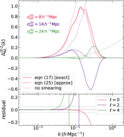
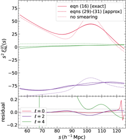
Figure 1: Multipoles of the non-linearly evolved redshift space dimensionless power spectrum (left panel) and 2pcf (right panel) in the DESI LRG configuration (Table 1). In each upper panel, solid curves show the exact result assuming scale-independent bias and ignoring mode coupling, dashed curves show the Zel’dovich smearing approximation, and dotted curves show the limit of no smearing; it is the obvious differences between these and the other curves which motivates Laguerre reconstruction. The text labels in the left upper panel give the estimated input values of $\sigma_{\rm eff}^{(\ell)}$ (equation 27) for this configuration. The solid curves in the lower panels show the corresponding residuals (i.e., approximate/exact - 1), while the horizontal dotted lines indicate $\pm 5\%$ deviations. See text for a discussion.

To simplify equation (17), we start by noting the identity

$$\left(1+\beta\mu_{k}^{2}\right)^{2}=\sum_{\ell}\,\chi_{\ell}(\beta)\,\mathcal{P}_{\ell}(\mu_{k})\,,$$ (19)

where, following Hamilton (1992), we defined

$$\chi_{0}(\beta) \equiv 1+\frac{2\beta}{3}+\frac{\beta^{2}}{5}\,,$$

$$\chi_{2}(\beta) \equiv 4\beta\left(\frac{1}{3}+\frac{\beta}{7}\right)\,,$$

$$\chi_{4}(\beta) \equiv\frac{8\beta^{2}}{35}\,.$$ (20)

Next, we use the fact that we are only interested in redshift space separations close to the BAO feature, so that $s\sim 100h^{-1}{\rm Mpc}$, while the bulk flow smearing scale $\sigma_{\rm v}\sim 10h^{-1}{\rm Mpc}$, so that $\sigma_{\rm v}/s\ll 1$. Since the Bessel functions in equation (16) effectively restrict the integral over $k$ to values $k\lesssim 1/s$, in equation (17) we can safely assume $K^{2}\ll 1$, so that ${\rm e}^{-K^{2}\mu_{k}^{2}}=1-K^{2}\mu_{k}^{2}+\mathcal{O}(K^{4})$ under the integral over $\mu_{k}$ (since $|\mu_{k}|\leq 1$). Finally, we use equations (3) and (4) to obtain the identity

$$(2\ell+1)\int_{-1}^{1}\frac{{\rm d}\mu}{2}\,\mathcal{P}_{\ell}(\mu)\,\mathcal{P}_{\ell^{\prime}}(\mu)\,\mu^{2}$$

$$\phantom{(2\ell+1)}=\frac{1}{3}\left[\delta_{\ell,\ell^{\prime}}+2(2\ell+1)\begin{pmatrix}\ell&\ell^{\prime}&2\\ 0&0&0\end{pmatrix}^{2}\right]\,.$$ (21)

Putting all this together, the integral in equation (17) becomes

$$(2\ell+1)\int_{-1}^{1}\frac{{\rm d}\mu_{k}}{2}\,\mathcal{P}_{\ell}(\mu_{k})\left(1+\beta\mu_{k}^{2}\right)^{2}{\rm e}^{-K^{2}\mu_{k}^{2}}$$

$$\phantom{2\ell}=\chi_{\ell}(\beta)\bigg{[}1-\frac{K^{2}}{3}\left\{1+\frac{2(2\ell+1)}{\chi_{\ell}(\beta)}\sum_{\ell^{\prime}}\chi_{\ell^{\prime}}(\beta)\begin{pmatrix}\ell&\ell^{\prime}&2\\ 0&0&0\end{pmatrix}^{2}\right\}$$

$$\phantom{2\ell\sum_{\ell^{\prime}}\chi_{\ell^{\prime}}(\beta)\delta_{\ell\ell^{\prime}}}+\mathcal{O}(K^{4})\bigg{]}$$

$$\phantom{2\ell}=\chi_{\ell}(\beta)\exp\left[-\frac{K^{2}}{3}\left(1+\frac{2(2\ell+1)}{\chi_{\ell}(\beta)}\sum_{\ell^{\prime}}\mathcal{C}_{\ell\ell^{\prime}}\chi_{\ell^{\prime}}(\beta)\right)\right]$$

$$\phantom{\chi_{\ell}(\beta)\exp[]}\times\left(1+\mathcal{O}(K^{4})\right)\,,$$ (22)

where, in the last equality, we defined the symmetric matrix $\mathcal{C}_{\ell\ell^{\prime}}$,

$$\mathcal{C}_{\ell\ell^{\prime}}\equiv\begin{pmatrix}\ell&\ell^{\prime}&2\\ 0&0&0\end{pmatrix}^{2}\,,$$ (23)

with $\ell$ and $\ell^{\prime}$ taking values $0,2,4$. Evaluating $\mathcal{C}_{\ell\ell^{\prime}}$ for these values using the definition of the Wigner $3j$ symbols gives

$$\mathcal{C}_{\ell\ell^{\prime}}=\begin{pmatrix}\mathcal{C}_{00}&\mathcal{C}_{02}&\mathcal{C}_{04}\\ \mathcal{C}_{20}&\mathcal{C}_{22}&\mathcal{C}_{24}\\ \mathcal{C}_{40}&\mathcal{C}_{42}&\mathcal{C}_{44}\end{pmatrix}=\begin{pmatrix}0&1/5&0\\ 1/5&2/35&2/35\\ 0&2/35&20/693\end{pmatrix}\,.$$ (24)

The expression for $\Delta^{(\ell)2}_{\rm NL}(k)$ in equation (17) simplifies to

$$\Delta^{(\ell)2}_{\rm NL}(k)=\Delta_{\rm lin}^{2}(k)\,b_{\rm eff}^{(\ell)2}\,{\rm e}^{-k^{2}\sigma_{\rm eff}^{(\ell)2}/2}\left(1+\mathcal{O}(K^{4})\right)\,,$$ (25)

where we defined the effective bias $b_{\rm eff}^{(\ell)}$ and effective smearing scale $\sigma_{\rm eff}^{(\ell)}$ using

$$b_{\rm eff}^{(\ell)2} \equiv b^{2}\,\chi_{\ell}(\beta)\,,$$ (26)

$$\sigma_{\rm eff}^{(\ell)2} \equiv 2\,\sigma_{\rm v}^{2}\left[1+\frac{f(f+2)}{3}\left(1+\frac{2(2\ell+1)}{\chi_{\ell}(\beta)}\sum_{\ell^{\prime}}\mathcal{C}_{\ell\ell^{\prime}}\,\chi_{\ell^{\prime}}(\beta)\right)\right]\,.$$ (27)

In effect, we have dealt with the fact that $\exp(-K^{2}\mu_{k}^{2})$ has alternating signs by evaluating the integral to lowest order in $K^{2}$, and then used the result to define an effective smearing scale. As a result, upto terms of order $\mathcal{O}(K^{4})$, the Fourier transform of $\Delta^{(\ell)2}_{\rm NL}(k)/k^{3}$ is explicitly an isotropic Gaussian smearing of the linear 2pcf with the replacements $b\to b_{\rm eff}^{(\ell)}$ and $2\sigma_{\rm v}^{2}\to\sigma_{\rm eff}^{(\ell)2}$ in equations (6) and (8). For $\ell=0$, this recovers the derivation of $\xi_{\rm NL}^{(0)}(s)$ in Nikakhtar et al. (2021b). For $\ell=2,4$, however, the presence of $j_{2}$ and $j_{4}$ in (16) means that the Fourier transform of $\Delta^{(\ell)2}_{\rm NL}(k)/k^{3}$ does not directly appear in $\xi_{\rm NL}^{(2)}$ and $\xi_{\rm NL}^{(4)}$.

To proceed further, we manipulate the Bessel functions to simplify the expressions for $\xi_{\rm NL}^{(\ell)}$ as described in Appendix A.1. As we show there, it is useful to define the quantity

$$\xi_{0}(s|\sigma)\equiv\int{\rm d}\ln k\,j_{0}(ks)\,\Delta_{\rm lin}^{2}(k)\,{\rm e}^{-k^{2}\sigma^{2}/2}\,,$$ (28)

which is exactly of the form for $\xi_{\rm NL}^{(0)}$, except that the Gaussian smearing uses the generic scale $\sigma$. In terms of this, the smearing approximation reduces to

$$\xi_{\rm NL}^{(0)}(s) =b_{\rm eff}^{(0)2}\,\xi_{0}(s|\sigma_{\rm eff}^{(0)})\,,$$ (29)

$$\xi_{\rm NL}^{(2)}(s) =b_{\rm eff}^{(2)2}\left[\xi_{0}(s|\sigma_{\rm eff}^{(2)})-\bar{\xi}_{0}(s|\sigma_{\rm eff}^{(2)})\right]\,,$$ (30)

$$\xi_{\rm NL}^{(4)}(s) =b_{\rm eff}^{(4)2}\left[\xi_{0}(s|\sigma_{\rm eff}^{(4)})+\frac{5}{2}\bar{\xi}_{0}(s|\sigma_{\rm eff}^{(4)})-\frac{7}{2}\bar{\bar{\xi}}_{0}(s|\sigma_{\rm eff}^{(4)})\right]\,,$$ (31)

where ${\bar{\xi}}_{0}(s|\sigma)$ and ${\bar{\bar{\xi}}}_{0}(s|\sigma)$ are defined in equation (68) and equation (69), respectively. Note especially the appearance of $\sigma_{\rm eff}^{(\ell)}$ in the expression for $\xi_{\rm NL}^{(\ell)}$, for each $\ell$. We refer to equations (29)-(31) as our Zel’dovich smearing approximation in what follows. In the limit of no smearing ($\sigma_{\rm eff}^{(l)}\to 0$) these expressions reduce to equations (6-8) of Hamilton (1992).

2.2 Accuracy of the smearing approximation

If the effects of mode coupling and scale-dependent bias can be ignored, the key step that allows us to approximate equation (16) by equations (29)-(31) (equivalently, equation 17 by equation 25) is the assumption that terms of order $\mathcal{O}(K^{4})$ in equation (25) can be approximately resummed into an exponential smearing term. There are several aspects of this approximation that bear some discussion.

The left panel of Fig. 1 compares the full integral expression (17) for $\Delta^{(\ell)2}_{\rm NL}$ (solid) with the no smearing limit (dotted) and our Zel’dovich smearing approximation (25) (dashed) in the DESI LRG configuration described later, for $\ell=0,2$ and $4$. The dotted curves have the same shape but different amplitudes ($\propto b_{\rm eff}^{(\ell)2}$). At each $\ell$, they are similar to the solid curves only at very small $k$, but they are otherwise very different: this is why some accounting for the smearing must be made. The dashed curves show that our approximation (25) fares much better. It loses fidelity at increasingly smaller $k$ as $\ell$ increases, with $\sim 5\%$ inaccuracies being reached at $k\simeq 0.17,0.07,0.035\,h\,{\rm Mpc}^{-1}$ for $\ell=0,2,4$, respectively. This is essentially a consequence of the fact that, having repackaged the $\mathcal{O}(K^{2})$ term into an exponential, the resulting $\sigma_{\rm eff}^{(\ell)}$ increases with $\ell$ (see the text labels in the left panel of Fig. 1). For comparison, $\sqrt{2}\sigma_{\rm v}\simeq 5.6h^{-1}{\rm Mpc}$ for this choice of parameters. In addition, this repackaging fails badly at large $k$, since it cannot reproduce the fact that, for $\ell=2$ and 4, the ‘exact’ result changes sign. (Note, however, that the ‘exact’ result ignores the effects of mode coupling and scale-dependent bias, both of which likely matter at large $k$.)

To see how this affects the BAO feature in configuration space, the right panel of Fig. 1 compares the full integral (16) for $\xi_{\rm NL}^{(\ell)}(s)$ (solid) with the no-smearing limit (dotted), and the smearing approximation in equations (29)-(31) (dashed). The latter was numerically evaluated using the identities (70). In this case, the no-smearing limit is again quite bad for all $\ell$, whereas our smearing approximation for $\xi_{\rm NL}^{(0)}$ is accurate at better than $\sim 1\%$ over nearly the entire range of scales of interest, failing in a relative sense only in the near vicinity of the zero-crossing of the function ($s\sim 123h^{-1}{\rm Mpc}$). The approximation for $\xi_{\rm NL}^{(2)}$ is accurate at better than $\sim 5\%$ over the entire range. While this level of agreement is remarkable, it is also clear that the approximation does not capture the oscillatory features of wavelength $\lambda_{\rm osc}\sim 30h^{-1}{\rm Mpc}$ seen near the BAO feature in the exact integral. These oscillations can be traced to the behaviour of the solid purple curve for $\Delta^{(2)2}_{\rm NL}(k)$ in the left panel, which has a (negative) spike in power at $k\sim 0.2\,h\,{\rm Mpc}^{-1}\approx 2\pi/\lambda_{\rm osc}$. The smearing approximation (dashed purple) has $\sigma_{\rm eff}^{(2)}\simeq 14h^{-1}{\rm Mpc}$, which understandably washes over the oscillations and cannot reproduce the change in sign of the $k$-space power. Finally, the approximation for $\xi_{\rm NL}^{(4)}$, although very close to the exact integral in an absolute sense, shows $>20\%$ deviations at $s<95h^{-1}{\rm Mpc}$. This is not surprising, considering that we saw $\gtrsim 5\%$ inaccuracies in the corresponding $k$-space approximation at $k\gtrsim 0.035\,h\,{\rm Mpc}^{-1}$ in the left panel.

This comparison suggests that, in practice, while the smearing approximation (29) for $\xi_{\rm NL}^{(0)}$ is expected to be very accurate near the BAO feature, the approximation for $\xi_{\rm NL}^{(2)}$ is likely to introduce biases when the observational errors on $\xi_{\rm NL}^{(2)}$ approach $\sim 5\%\,\times\sqrt{N}$ for $N$ independent measurements. Similarly, for $\xi_{\rm NL}^{(4)}$, the increasing inaccuracy of the model at $s\lesssim 90h^{-1}{\rm Mpc}$ makes it likely that accurate measurements of $\xi_{\rm NL}^{(4)}$ could introduce biases in the inferred parameters.

Another consequence of the $\ell$-dependence of $\sigma_{\rm eff}^{(\ell)}$ is that the steepness of the increase with $\ell$ is especially pronounced for highly biased tracers, for which $\beta$ can be small. This is quite different from the $\ell=0$ behaviour, because $\chi_{\ell}(\beta)\to 1$ in the denominator of the last term in equation (27) for $\ell=0$ but diverges for other $\ell$, if $\beta\to 0$. This can potentially complicate the Laguerre reconstruction described in section 3, for which a useful rule of thumb is that the BAO feature should be about one smearing length away from the smallest and largest scales being modelled.

The level to which these inaccuracies in the model affect parameter recovery will depend on the details of the survey in question. We return to this point in section 5 where we show results for two mock survey configurations.

3 Multipole reconstruction

If we model the real space linear theory 2pcf $\xi_{\rm lin}(r)$ in some range $r_{\rm min}\leq r\leq r_{\rm max}$ as the simple polynomial of degree $M-1$,

$$b^{2}\xi_{\rm lin}(r)=\sum_{m=0}^{M-1}\frac{a_{m}}{m!}\left(\frac{r}{\sigma_{\rm fid}}\right)^{m}\,,$$ (32)

where $\sigma_{\rm fid}$ is a fiducial scale used to non-dimensionalise the problem, then the Gaussian convolution $\xi_{0}(s|\sigma)$ becomes

$$b^{2}\xi_{0}(s|\sigma)=\sum_{m=0}^{M-1}\frac{a_{m}}{m!}\left(\frac{\sigma}{\sigma_{\rm fid}}\right)^{m}\,\mu_{m}(s/\sigma)\,,$$ (33)

in a corresponding range $s_{\rm min}\leq s\leq s_{\rm max}$, where the $\mu_{m}(x)$ are given by equation (7) of Nikakhtar et al. (2021a) in terms of generalised Laguerre functions.

PS22 exploited the fact that, when focusing on the redshift space monopole $\xi_{\rm NL}^{(0)}$ and fixing the smearing scale $\sigma=\sigma_{\rm eff}^{(0)}$, the coefficients $\mathbf{a}$ give a representation of the un-smeared real space linear 2pcf in some chosen range of scales. If we think of this as saying that the coefficients $\mathbf{a}$ describe the behaviour of (the Fourier transform of) $\Delta_{\rm lin}^{2}(k)/k^{3}$, then the derivation in section 2 shows that it is only the value of the smearing scale in the factor $\sim{\rm e}^{-k^{2}\sigma^{2}/2}$ which changes when considering different multipoles. This means that the same polynomial coefficients $\mathbf{a}$ should give a good description of all multipoles $\xi_{\rm NL}^{(\ell)}$, $\ell=0,2,4$, provided one appropriately modifies the smearing scale (i.e., uses $\sigma=\sigma_{\rm eff}^{(\ell)}$) and propagates the effect of volume averaging of the resulting Laguerre functions. In this case, $b$, $\beta$ and $\sigma_{\rm v}$ would be free parameters that must be jointly constrained with $\mathbf{a}$. The fact that the polynomial description of the linear 2pcf is only valid over a finite range of scales $s_{\rm min}\leq s\leq s_{\rm max}$ can be accounted for by introducing three new free parameters, which would capture the (constant) integrals of $u^{2}\xi_{0}(u|\sigma_{\rm eff}^{(2)})$, $u^{2}\xi_{0}(u|\sigma_{\rm eff}^{(4)})$ and $u^{4}\xi_{0}(u|\sigma_{\rm eff}^{(4)})$ over the range $0\leq u\leq s_{\rm min}$.

In this section, we describe how to implement this approach. In addition to the linear point $r_{\rm LP}$, this approach can potentially constrain the cosmological parameters $\beta$ and $\sigma_{\rm v}$ without assuming any fiducial cosmology. We will also discuss the role of the linear bias parameter $b$, whose effect in the model is challenging to disentangle from the coefficients $\mathbf{a}$ (but which does not affect the recovery of the linear point).

3.1 Laguerre model for 2pcf multipoles

In practice, it is convenient to choose $\sigma_{\rm fid}$ and the range $\{s_{\rm min},s_{\rm max}\}$ over which to assume equation (32), based on the observed location and width of the BAO feature in the monopole data, so that $\sigma_{\rm fid}\simeq 10h^{-1}{\rm Mpc}$ and $\{s_{\rm min},s_{\rm max}\}\simeq\{60,120\}h^{-1}{\rm Mpc}$. While the value of $\sigma_{\rm fid}$ mainly affects numerical stability and does not change any of the results, the final constraints on the parameters $\mathbf{a}$ are mildly sensitive to the choice of $\{s_{\rm min},s_{\rm max}\}$ (see PS22, for a discussion).

The expressions for $\xi_{\rm NL}^{(\ell)}(s)$ with $\ell=2,4$ depend on volume integrals of $\xi_{0}$ from $0$ to $s$, while the Laguerre expansion for $\xi_{0}$ is only valid in the range $s_{\rm min}\leq s\leq s_{\rm max}$. To account for this, we introduce three new free parameters $\bar{Q}^{(2)}_{2}$, $\bar{Q}^{(4)}_{2}$ and $\bar{Q}^{(4)}_{4}$, defined by

$$\bar{Q}^{(\ell)}_{j}\equiv b^{2}\,\frac{(j+1)}{s_{\rm min}^{j+1}}\int_{0}^{s_{\rm min}}{\rm d}u\,u^{j}\,\xi_{0}(u|\sigma_{\rm eff}^{(\ell)})\,,$$ (34)

so that

$$\bar{Q}^{(2)}_{2} =b^{2}\,\bar{\xi}_{0}(s_{\rm min}|\sigma_{\rm eff}^{(2)})\,,$$

$$\bar{Q}^{(4)}_{2} =b^{2}\,\bar{\xi}_{0}(s_{\rm min}|\sigma_{\rm eff}^{(4)})\,,$$

$$\bar{Q}^{(4)}_{4} =b^{2}\,\bar{\bar{\xi}}_{0}(s_{\rm min}|\sigma_{\rm eff}^{(4)})\,,$$ (35)

and define the volume averages of the $\mu_{m}(x)$ as

$$\bar{\mu}_{m}(s;\sigma) \equiv\frac{3}{s^{3}}\int_{s_{\rm min}}^{s}{\rm d}u\,u^{2}\,\mu_{m}(u/\sigma)\,,$$ (36)

$$\bar{\bar{\mu}}_{m}(s;\sigma) \equiv\frac{5}{s^{5}}\int_{s_{\rm min}}^{s}{\rm d}u\,u^{4}\,\mu_{m}(u/\sigma)\,.$$ (37)

Since the lower integration limits in these expressions are $s_{\rm min}$ rather than $0$, we clearly have $\bar{\mu}_{m}(s_{\rm min};\sigma)=0=\bar{\bar{\mu}}_{m}(s_{\rm min};\sigma)$. Using equations (33), (36) and (37) to construct $\bar{\xi}_{0}$ and $\bar{\bar{\xi}}_{0}$, we can model $\xi_{\rm NL}^{(\ell)}(s)$ (equations 29-31) in the range $s_{\rm min}\leq s\leq s_{\rm max}$ as

$$\xi_{\rm NL}^{(0)}(s) =\chi_{0}\,\sum_{m=0}^{M-1}\frac{a_{m}}{m!}\left(\frac{\sigma_{\rm eff}^{(0)}}{\sigma_{\rm fid}}\right)^{m}\mu_{m}(s/\sigma_{\rm eff}^{(0)})\,,$$ (38)

$$\xi_{\rm NL}^{(2)}(s) =-\chi_{2}\bigg{[}\bar{Q}^{(2)}_{2}\left(\frac{s_{\rm min}}{s}\right)^{3}$$

$$\phantom{b}-\sum_{m=0}^{M-1}\frac{a_{m}}{m!}\left(\frac{\sigma_{\rm eff}^{(2)}}{\sigma_{\rm fid}}\right)^{m}\bigg{\{}\mu_{m}(s/\sigma_{\rm eff}^{(2)})-\bar{\mu}_{m}(s;\sigma_{\rm eff}^{(2)})\bigg{\}}\bigg{]}\,,$$ (39)

$$\xi_{\rm NL}^{(4)}(s) =\chi_{4}\bigg{[}\frac{5}{2}\,\bar{Q}^{(4)}_{2}\left(\frac{s_{\rm min}}{s}\right)^{3}-\frac{7}{2}\,\bar{Q}^{(4)}_{4}\left(\frac{s_{\rm min}}{s}\right)^{5}$$

$$\phantom{-b^{2}}+\sum_{m=0}^{M-1}\frac{a_{m}}{m!}\left(\frac{\sigma_{\rm eff}^{(4)}}{\sigma_{\rm fid}}\right)^{m}\bigg{\{}\mu_{m}(s/\sigma_{\rm eff}^{(4)})$$

$$\phantom{+\sum a_{m}()^{4}}+\frac{5}{2}\,\bar{\mu}_{m}(s;\sigma_{\rm eff}^{(4)})-\frac{7}{2}\,\bar{\bar{\mu}}_{m}(s;\sigma_{\rm eff}^{(4)})\bigg{\}}\bigg{]}\,,$$ (40)

where the prefactors only involve $\chi_{\ell}$ since we absorbed $b^{2}$ into the coefficients $\mathbf{a}$ and the definition of $\bar{Q}^{(\ell)}_{j}$.

To decrease the number of free parameters, we exploit the fact that $\bar{Q}^{(2)}_{2}$ and $\bar{Q}^{(4)}_{2}$ only appear with the combination $(s_{\rm min}/s)^{3}$, and work with the quantities $\Delta\xi_{\rm NL}^{(\ell)}(s)$ defined by

$$\Delta\xi_{\rm NL}^{(\ell)}(s)\equiv\xi_{\rm NL}^{(\ell)}(s)-g_{\ell}\,(s_{\rm min}/s)^{3}\,\xi_{\rm NL}^{(\ell)}(s_{\rm min})\,,$$ (41)

where $g_{0}=0$ and $g_{2}=1=g_{4}$. The models for these quantities are

$$\Delta\xi_{\rm NL}^{(0)}(s) =\chi_{0}\bigg{[}\sum_{m=0}^{M-1}\frac{a_{m}}{m!}\left(\frac{\sigma_{\rm eff}^{(0)}}{\sigma_{\rm fid}}\right)^{m}\mu_{m}(s/\sigma_{\rm eff}^{(0)})\bigg{]}\,,$$ (42)

$$\Delta\xi_{\rm NL}^{(2)}(s) =\chi_{2}\bigg{[}\sum_{m=0}^{M-1}\frac{a_{m}}{m!}\left(\frac{\sigma_{\rm eff}^{(2)}}{\sigma_{\rm fid}}\right)^{m}\bigg{\{}\mu_{m}(s/\sigma_{\rm eff}^{(2)})$$

$$\phantom{\chi_{2}\,\sum_{m=0}^{M-1}}-(s_{\rm min}/s)^{3}\,\mu_{m}(s_{\rm min}/\sigma_{\rm eff}^{(2)})-\bar{\mu}_{m}(s;\sigma_{\rm eff}^{(2)})\bigg{\}}\bigg{]}\,,$$ (43)

$$\Delta\xi_{\rm NL}^{(4)}(s) =\chi_{4}\bigg{[}\frac{7}{2}\bar{Q}^{(4)}_{4}\left(\frac{s_{\rm min}}{s}\right)^{3}\left(1-\left(\frac{s_{\rm min}}{s}\right)^{2}\right)$$

$$\phantom{\frac{7}{2}\bar{q}^{(4)}_{4}}+\sum_{m=0}^{M-1}\frac{a_{m}}{m!}\left(\frac{\sigma_{\rm eff}^{(4)}}{\sigma_{\rm fid}}\right)^{m}\bigg{\{}\mu_{m}(s/\sigma_{\rm eff}^{(4)})$$

$$\phantom{\frac{7}{2}\bar{q}^{(4)}_{4}\frac{a_{m}}{m!}}-(s_{\rm min}/s)^{3}\,\mu_{m}(s_{\rm min}/\sigma_{\rm eff}^{(4)})$$

$$\phantom{\frac{7}{2}\bar{q}^{(4)}_{4}\frac{a_{m}}{m!}}+\frac{5}{2}\bar{\mu}_{m}(s;\sigma_{\rm eff}^{(4)})-\frac{7}{2}\bar{\bar{\mu}}_{m}(s;\sigma_{\rm eff}^{(4)})\bigg{\}}\bigg{]}\,,$$ (44)

which eliminates the parameters $\bar{Q}^{(2)}_{2}$ and $\bar{Q}^{(4)}_{2}$. The final dimensionality of our model is then $M+3$ when only using the monopole and quadrupole and $M+4$ when using all $\ell=0,2,4$. Since $\Delta\xi_{\rm NL}^{(\ell)}(s_{\rm min})=0$ by construction, we delete the corresponding two data points for $\ell=2$ and $4$ from the data set after constructing $\Delta\xi_{\rm NL}^{(\ell)}(s)$ from the observed $\xi_{\rm NL}^{(\ell)}(s)$.

Written like this, the model explicitly depends on the parameter $b$ only through the definitions of $\sigma_{\rm eff}^{(\ell)2}$ which contain factors of $f=b\,\beta$. Since this dependence is quite weak, we include in our data set a measurement of the integral $\Sigma_{\rm obs}^{2}$ of the monopole power spectrum in linearly spaced bins of $\mathbf{k}$,

$$\hat{\Sigma}_{\rm obs}^{2}\equiv\frac{\Delta k}{6\pi^{2}}\sum_{i}\,P^{(0)}(k_{i})\,,$$ (45)

which we model using

$$\Sigma_{\rm obs}^{2} =\frac{1}{3}\int{\rm d}\ln k\,k^{-2}\,\Delta^{(0)2}_{\rm NL}(k)$$

$$\approx\frac{1}{3}\,b_{\rm eff}^{(0)2}\int{\rm d}\ln k\,k^{-2}\,\Delta_{\rm lin}^{2}(k)\,{\rm e}^{-k^{2}\sigma_{\rm eff}^{(0)2}/2}$$

$$\approx b^{2}\,\chi_{0}(\beta)\,\sigma_{\rm v}^{2}\,.$$ (46)

For the BOSS Final Year cosmology, the model approximation in the last line gives $\Sigma_{\rm obs}=10.9\,(10.0)\,h^{-1}{\rm Mpc}$, compared to $9.3\,(8.4)\,h^{-1}{\rm Mpc}$ from the exact integral in the first line for DESI (BOSS DR12) LRGs, an overestimate by $\sim 17\%\,(19\%)$. We therefore divide the last line of (46) by $1.38$ to account for the overestimate,

$$\Sigma_{\rm obs,model}^{2}=b^{2}\,\chi_{0}(\beta)\,\sigma_{\rm v}^{2}\,/\,1.38\,.$$ (47)

We discuss this limitation of our model in section 5.2 below.

3.2 Gauss-Poisson covariance matrix

For simplicity, in this work we use the Gauss-Poisson approximation to model the covariance matrix of our mock observations. This can be easily replaced with more accurate covariance matrix estimates based on simulations or mock galaxy catalogs, as needed (e.g., Chuang et al., 2015; Zhao et al., 2021).

In the Gauss-Poisson approximation, the covariance matrix

$$C^{\ell\ell^{\prime}}_{ij}\equiv\left\langle\,\xi_{\rm NL}^{(\ell)}(s_{i})\xi_{\rm NL}^{(\ell^{\prime})}(s_{j})\,\right\rangle-\left\langle\,\xi_{\rm NL}^{(\ell)}(s_{i})\,\right\rangle\left\langle\,\xi_{\rm NL}^{(\ell^{\prime})}(s_{j})\,\right\rangle$$ (48)

can be written as (e.g. Grieb et al., 2016),

$$C^{\ell\ell^{\prime}}_{ij}=\frac{i^{\ell_{1}+\ell_{2}}}{2\pi^{2}}\int dk\,k^{2}\,{\bar{j}}_{\ell_{1}}(ks_{i})\,{\bar{j}}_{\ell_{2}}(ks_{j})\,\sigma^{2}_{\ell_{1}\ell_{2}}(k)\,,$$ (49)

where

$$\sigma^{2}_{\ell_{1}\ell_{2}}(k) =\frac{(2\ell_{1}+1)(2\ell_{2}+1)}{V_{\rm sur}/2}$$

$$\phantom{V_{sur}/2}\times\int_{-1}^{1}\frac{d\mu}{2}\,\left[P(k,\mu)+\frac{1}{\bar{n}}\right]^{2}\,\mathcal{P}_{\ell_{1}}(\mu)\,\mathcal{P}_{\ell_{2}}(\mu)$$ (50)

for a survey of volume $V_{\rm sur}$ with observed tracer number density $\bar{n}$, and

$${\bar{j}}_{\ell}(ks_{i})=\frac{4\pi}{V_{i}}\int ds\,s^{2}\,j_{\ell}(ks)\,W_{i}(s)$$ (51)

with

$$V_{i}=4\pi\int ds\,s^{2}\,W_{i}(s)\,,$$ (52)

where $W_{i}(s)$ describes the shape of a window over which $j_{\ell}$ has been averaged. E.g., for the tophat bins of width $\Delta s$ centered on $s_{i}$ that we use, $W_{i}(s)=1$ if $s_{i}-\Delta s/2\leq s\leq s_{i}+\Delta s/2$, and the integral which defines $\bar{j}_{\ell}$ can be done analytically.

Since we use $\Delta\xi_{\rm NL}^{(\ell)}$ (equations 42-44) as our observables instead of $\xi_{\rm NL}^{(\ell)}$, the covariance matrix $C^{\ell\ell^{\prime}}_{ij}$ used in the likelihood evaluation must be replaced with

$$\Delta C^{\ell\ell^{\prime}}_{ij} =C^{\ell\ell^{\prime}}_{ij}-g_{\ell}\left(\frac{s_{1}}{s_{i}}\right)^{3}C^{\ell\ell^{\prime}}_{1j}-g_{\ell^{\prime}}\left(\frac{s_{1}}{s_{j}}\right)^{3}C^{\ell\ell^{\prime}}_{i1}$$

$$\phantom{C^{\ell\ell^{\prime}}_{ij}-g_{\ell^{\prime}}}+g_{\ell}\,g_{\ell^{\prime}}\left(\frac{s_{1}^{2}}{s_{i}s_{j}}\right)^{3}C^{\ell\ell^{\prime}}_{11}\,,$$ (53)

where we assumed $s_{1}=s_{\rm min}$ and it is understood that we discard the rows and columns corresponding to $s=s_{\rm min}$ for $\ell=2$ and $\ell=4$.

Finally, when including in the data set a measurement $\Sigma_{\rm obs}^{2}$ (equation 45), we must modify the covariance matrix further, by including a row and column accounting for the error in $\Sigma_{\rm obs}^{2}$ and its covariance with the measured $\xi_{\rm NL}^{(\ell)}(s)$ in bins of $s$. In the Gauss-Poisson approximation, these are respectively given by

$${\rm Var}\left(\hat{\Sigma}_{\rm obs}^{2}\right)=\frac{8\Delta k^{2}}{9}\sum_{i}\frac{1}{V_{k_{i}}^{2}}\int_{k_{i}-\Delta k/2}^{k_{i}+\Delta k/2}{\rm d}k\,k^{2}\sigma^{2}_{00}(k)\,,$$ (54)

$${\rm Cov}\left(\hat{\Sigma}_{\rm obs}^{2},\xi_{\rm NL}^{(\ell)}(s_{j})\right)$$

$$=\frac{2\Delta k}{3\pi}\,i^{\ell}\sum_{i}\frac{1}{V_{k_{i}}}\int_{k_{i}-\Delta k/2}^{k_{i}+\Delta k/2}{\rm d}k\,k^{2}\,\bar{j}_{\ell}(ks_{j})\,\sigma^{2}_{0\ell}(k)\,,$$ (55)

where $V_{k_{i}}=(4\pi/3)[(k_{i}+\Delta k/2)^{3}-(k_{i}-\Delta k/2)^{3}]$ and $\sigma^{2}_{\ell_{1}\ell_{2}}(k)$ and $\bar{j}_{\ell}(ks_{j})$ are defined in equations (50) and (51), respectively. To calculate the covariance of $\hat{\Sigma}_{\rm obs}^{2}$ with $\Delta\xi_{\rm NL}^{(\ell)}$ instead of $\xi_{\rm NL}^{(\ell)}$, we simply subtract $g_{\ell}(s_{1}/s_{j})^{3}{\rm Cov}(\hat{\Sigma}_{\rm obs}^{2},\xi_{\rm NL}^{(\ell)}(s_{1}))$ from equation (55) and delete the entries corresponding to $s_{1}=s_{\rm min}$ as before.

4 Analysis

We use mock data generated assuming two choices of sample: (i) a BOSS DR12 LRG-like sample and (ii) a DESI LRG-like sample. In each case, we define a multivariate Gaussian using equation (16) and the first line of equation (46) as the mean, and equations (49), (54) and (55) with tophat binning as the covariance matrix. The corresponding choices of the survey redshift $z_{\rm sur}$, effective survey volume $V_{\rm sur}$, galaxy number density $\bar{n}$ and linear halo bias $b$ are summarised in Table 1. For each survey choice, we draw one realisation from the corresponding multivariate Gaussian and construct the observables $\Delta\xi_{\rm NL}^{(\ell)}(s)$ using equation (41) for $55h^{-1}{\rm Mpc}\leq s\leq 125h^{-1}{\rm Mpc}$ in $72$ linearly spaced, $\simeq 1h^{-1}{\rm Mpc}$ wide bins, along with $\hat{\Sigma}_{\rm obs}^{2}$ in linearly spaced bins $k_{\rm min}<k_{i}<0.5\,h\,{\rm Mpc}^{-1}$ with spacing $\Delta k=k_{\rm min}/2$, where $k_{\rm min}=2\times 2\pi/V_{\rm sur}^{1/3}$. This gives 84 (189) $k$-bins for the BOSS DR12 (DESI) configuration.

The BOSS DR12 numbers in Table 1 are chosen to match the ‘Bin 3’ sample from Alam et al. (2015), while the DESI LRG numbers are consistent with DESI Collaboration et al. (2016, see their section 3.2) and Zhou et al. (2020). The linear binning choice of $k$-bins for the covariance of $\hat{\Sigma}_{\rm obs}^{2}$ is similar to that in fig. 3 of Beutler et al. (2014). All the results use the BOSS Final Year flat $\Lambda$CDM cosmology (Alam et al., 2017) with parameters as listed in the Introduction. The input (‘true’) values of $(f,\sigma_{\rm v})$ for the BOSS DR12 and DESI configurations are, respectively, $(0.790,4.19\,h^{-1}{\rm Mpc})$ and $(0.814,4.01\,h^{-1}{\rm Mpc})$.

mock	$z_{\rm sur}$	$V_{\rm sur}$	$\bar{n}$	$b$
sample		(${\rm Gpc}^{3}$)	$10^{-4}\,(h^{-1}{\rm Mpc})^{-3}$
BOSS DR12	$0.61$	$4.1$	$4.7$	$2.1$
DESI LRG	$0.7$	$45.3$	$6.0$	$2.435$

Table 1: Sample definitions for mock measurements. The columns give the assumed values of effective survey redshift $z_{\rm sur}$, survey volume $V_{\rm sur}$ in ${\rm Gpc}^{3}$, galaxy number density in $10^{-4}\,(h^{-1}{\rm Mpc})^{-3}$ and linear bias $b$, for the mock samples representing BOSS DR12 LRGs and DESI LRGs. See text for original references.

4.1 Bayesian sampling

In this section, we describe our setup for Bayesian sampling using the Markov Chain Monte Carlo (MCMC) technique to constrain the model parameters using the mock data described above.

4.1.1 Likelihood

We construct a Gaussian likelihood of the form ${\rm e}^{-\chi^{2}/2}$, with

$$\chi^{2}=(\mathbf{d}-\mathbf{m})^{\rm T}\,C^{-1}\,(\mathbf{d}-\mathbf{m})\,,$$ (56)

where $\mathbf{d}$ and $\mathbf{m}$ represent the data and model vector, respectively, and $C$ is the data covariance matrix.

The data vector $\mathbf{d}$ comprises the $\Delta\xi_{\rm NL}^{(\ell)}$ measurements and $\hat{\Sigma}_{\rm obs}^{2}$ as described above. For the BOSS DR12 configuration, we use $\ell=0$ and $2$ measurements for $\Delta\xi_{\rm NL}^{(\ell)}$, since $\ell=4$ is not measured with enough precision to yield useful information. For the DESI configuration, on the other hand, we use $\ell=0,2$ and $4$. Keeping in mind the deletion of data points when constructing $\Delta\xi_{\rm NL}^{(\ell)}$ from $\xi_{\rm NL}^{(\ell)}$ (see the discussion below equation 44), this leads to data vectors of length $144$ and $215$ for the BOSS DR12 and DESI configurations, respectively. The data covariance $C$ is correspondingly modelled by combining equations (53), (54) and (55), along with the modification discussed below equation (55).

The model vector $\mathbf{m}$ correspondingly comprises equations (42)-(44) for $\Delta\xi_{\rm NL}^{(\ell)}$ and equation (47) for $\Sigma_{\rm obs}^{2}$. For reasons we discuss below, we use a degree 7 polynomial ($M=8$) for the BOSS DR12 configuration to model the linear theory 2pcf in (32), while for the DESI configuration we use a degree 9 polynomial ($M=10$). Along with the three parameters $b$, $\beta$ and $\sigma_{\rm v}$, and the new parameter $\bar{Q}^{(4)}_{4}$ when using $\ell=4$ measurements, this leads to $133$ ($201$) degrees of freedom for the BOSS DR12 (DESI) configuration.

4.1.2 Eigen-coefficients and standardisation

Unlike PS22, we have chosen not to introduce an offset scale $r_{\rm fid}$ in equation (32) – which would replace $r^{m}\to(r-r_{\rm fid})^{m}$ – since this considerably simplifies the manipulations of the Laguerre functions $\mu_{m}(x)$. This, however, introduces strong degeneracies between the polynomial coefficients $\mathbf{a}$, because the 2pcf data lie very far from $r=0$. These degeneracies, if not handled carefully, render the MCMC sampling unstable.

To deal with this, we approximately decorrelate the polynomial coefficients prior to MCMC sampling, as follows. We first fix the parameters $(b,\beta,\sigma_{\rm v})$ to some fiducial values $(b_{\ast},\beta_{\ast},\sigma_{{\rm v}\ast})$ and analytically solve the linear Gaussian problem for the a posteriori distribution of $\mathbf{a}$ using the monopole data $\xi_{\rm NL}^{(0)}$ alone, exactly as described by PS22. Since this distribution is a multivariate Gaussian in $\mathbf{a}$, at this stage we obtain a mean vector $\mathbf{a}_{\ast}$ and an $M$-dimensional covariance matrix $C^{\rm(poly)}$ for the polynomial coefficients $\mathbf{a}$. The diagonalising rotation $R$ of $C^{\rm(poly)}$ then approximately decorrelates $\mathbf{a}$ by defining

$$\mathbf{e}=R^{\rm T}\cdot\mathbf{a}$$ (57)

Hereon, we refer to $\mathbf{e}$ as the eigen-coefficients corresponding to $\mathbf{a}$ even though, strictly speaking, this decorrelation is only approximate when we also vary $b,\beta,\sigma_{\rm v}$ below. We also emphasize that, although the rotation $R$ is defined for a specific choice of fiducial values $(b_{\ast},\beta_{\ast},\sigma_{{\rm v}\ast})$, this is a fixed rotation introduced purely for convenience. Our approach does not rely on these fiducial values being close to the ‘truth’; values very different from the underlying true model would only result in somewhat longer convergence times for the MCMC chains, but will not bias the final result.

Another issue we must deal with is that the typical values of the best fit eigen-coefficients span a large dynamic range of $\gtrsim 10^{8}$. To simplify the MCMC sampling, we therefore define the standardised eigen-coefficients $\tilde{\mathbf{e}}$ using

$$\tilde{e}_{m}=(e_{m}-\left\langle\,e\,\right\rangle_{m})/\sigma_{m}\,;\quad 0\leq m\leq M-1\,,$$ (58)

where $\left\langle\,e\,\right\rangle_{m}$ and $\sigma_{m}$ are the mean and standard deviation, respectively, of the $m^{\rm th}$ eigen-coefficient as obtained from the linear Gaussian analysis. Similarly, for convenience, we also standardise the parameters $(b,\beta,\sigma_{\rm v})$ by defining

$$\tilde{b}=b/b_{\ast}-1\,;\quad\tilde{\beta}=\beta/\beta_{\ast}-1\,;\quad\tilde{\sigma}_{\rm v}=\sigma_{\rm v}/\sigma_{{\rm v}\ast}-1\,,$$ (59)

although this is not as essential as the standardisation of $\mathbf{e}$, since the parameters $(b,\beta,\sigma_{\rm v})$ are typically of order unity. When including $\ell=4$ data, we similarly standardise $\bar{Q}^{(4)}_{4}$ using

$$\tilde{Q}^{(4)}_{4}=(\bar{Q}^{(4)}_{4}-Q_{\ast})/\sigma_{Q\ast}\,,$$ (60)

where $Q_{\ast}$ and $\sigma_{Q\ast}$ are respectively set equal to the expected typical value (we use $Q_{\ast}=0.008\times b_{\ast}^{2}$ throughout) and width of the prior range described later.

We set up the MCMC described below to sample the parameters $\{\tilde{\mathbf{e}},\tilde{b},\tilde{\beta},\tilde{\sigma}_{\rm v},[\tilde{Q}^{(4)}_{4}]\}$, but display all our final results in terms of $\{\mathbf{e},b,\beta,\sigma_{\rm v},[\bar{Q}^{(4)}_{4}]\}$ by simply undoing the standardisations.

4.1.3 Parameter priors

We define priors on the sampled parameters as follows.

For each eigen-coefficient $e_{m}$ with $0\leq m\leq M-1$, we use broad uniform priors in the range $e_{m}\in[\left\langle\,e_{m}\,\right\rangle-25\sigma_{m},\left\langle\,e_{m}\,\right\rangle+25\sigma_{m}]$, where $\left\langle\,e_{m}\,\right\rangle$ and $\sigma_{m}$ are obtained from the linear Gaussian analysis as described above. For the parameters $\beta$ and $\sigma_{\rm v}$, we use broad uniform priors over the ranges $\beta\in[-10,+10]$ and $\sigma_{\rm v}\in[0,+20]\,h^{-1}{\rm Mpc}$. When including $\ell=4$ data, we use a uniform prior on $\bar{Q}^{(4)}_{4}$ in the range $\bar{Q}^{(4)}_{4}\in[0,+0.1]\times b_{\ast}^{2}$ (so that $\sigma_{Q\ast}=0.1\,b_{\ast}^{2}$ in equation 60).

For the linear bias $b$, we will display results assuming a $10\%$ Gaussian prior, namely, a Gaussian distribution with mean $b_{\rm true}$ and standard deviation $0.1\,b_{\rm true}$, where $b_{\rm true}$ is the appropriate input value from Table 1. We discuss this choice further in section 5.2, and later also report results of relaxing the prior to be uniform in the range $b\in[-20,+20]$.

4.1.4 MCMC sampling

We use the publicly available Python-based framework cobaya (Torrado & Lewis, 2019, 2021) to perform MCMC sampling. We use the Theory class of cobaya to set up numerical evaluations of equations (42)-(44) and equation (47) for the model, and the Likelihood class to evaluate (56) for the the log-likelihood. Throughout, we sample the standardised parameters $\{\tilde{\mathbf{e}},\tilde{b},\tilde{\beta},\tilde{\sigma}_{\rm v},[\tilde{Q}^{(4)}_{4}]\}$, appropriately accounting for the standardisation in the model evaluation. We set the fiducial parameter values $(b_{\ast},\beta_{\ast},\sigma_{\rm v\ast})$ to the input values for each mock sample, namely, $(2.1,0.376,4.19h^{-1}{\rm Mpc})$ for BOSS DR12 LRGs and $(2.435,0.334,4.01h^{-1}{\rm Mpc})$ for DESI LRGs.

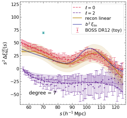
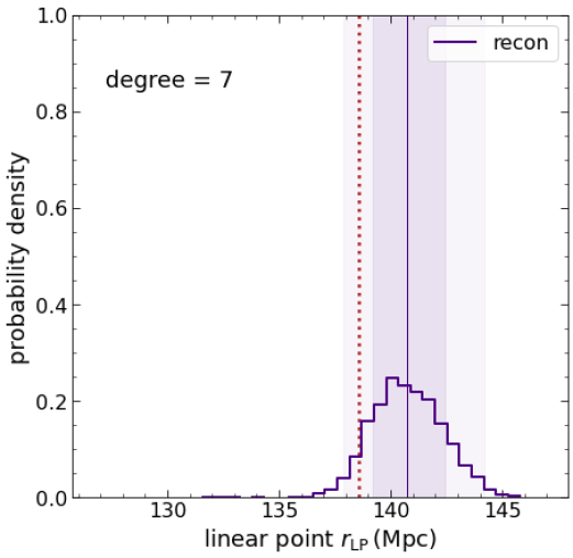
Figure 2: (Left panel): Comparison of mock data and best fit models for $s^{2}\Delta\xi_{\rm NL}^{(\ell)}(s)$ with $\ell=0,2$, along with $\Sigma_{\rm obs}^{2}$, for the mock BOSS DR12 data (Table 1) analysed with a degree 7 Laguerre function (section 3.1). Data points with errors show the mock measurements, dashed curves show the best fit model, with the shaded bands indicating the respective central $68\%$ confidence region. The single cyan data point with error bar shows the mock value of $\Sigma_{\rm obs}^{2}$, with the shaded cyan box (nearly indistinguishable from the data point), showing the value in the best fit model. Dotted curves show the input ‘truth’ used to generate the data as described in section 4. Yellow solid curve shows the reconstructed linear theory $\xi_{\rm L}$ using the best fit polynomial coefficients, with the inner (outer) yellow bands showing the central $68\%$ ($95\%$) confidence region. Blue solid curve shows the linear theory $\xi_{\rm L}=b^{2}\xi_{\rm lin}$ in the input cosmology. (Right panel): Recovery of the linear point $r_{\rm LP}$ for the same analysis. Histogram shows the inferred distribution of $r_{\rm LP}$, with the solid vertical line and inner (outer) vertical band showing the median and central $68\%$ ($95\%$) confidence region. Dotted red vertical line shows the value in the input cosmology. This figure can be compared with figs. 5 and 6 of PS22, where the analysis only used $\ell=0$ and did not vary the parameters $\{b,\beta,\sigma_{\rm v}\}$.

During the model evaluation, we internally scale all the data by a constant factor $10^{4}$ in order to numerically stabilise the initial linear Gaussian calculation (see PS22, for a discussion), and undo the scaling when presenting results. The likelihood calculation also enforces $f=b\,\beta\geq 0$, by returning zeros for all $\Delta\xi_{\rm NL}^{(\ell)}(s)$ otherwise. We use the mcmc sampler included in cobaya, which implements the Metropolis-Hastings algorithm. We initialise all chains by sampling narrow uniform distributions in each parameter, centered on the linear Gaussian result, and stop the chains when the Gelman-Rubin index $|R-1|$ falls below 0.05 for convergence of both, means as well as $95\%$ bounds. The MCMC chains are analysed using the Python package getdist (Lewis, 2019), discarding the first $30\%$ of the samples as burn-in.

5 Results

We now discuss the results of the MCMC analysis of the BOSS DR12 and DESI LRG mock data.

5.1 Parameter constraints

Fig. 2 shows the best fit $\Delta\xi_{\rm NL}^{(\ell)}(s)$ and and $\Sigma_{\rm obs}^{2}$ (left panel) and the inferred distribution of the linear point $r_{\rm LP}$ (right panel), by fitting a degree $7$ Laguerre function to the mock BOSS DR12 measurements for $\ell=0$ and $2$ (shown as the data points with errors). We discuss the choice of degree later.

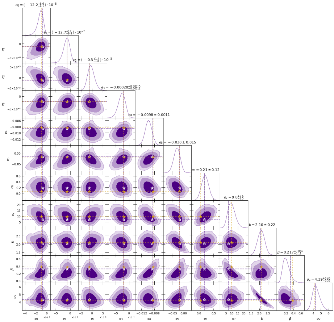
Figure 3: Joint a posteriori distributions of all (eigen)-parameters varied to obtain the results in Fig. 2 for the BOSS DR12 mock data set. Dashed purple lines intersecting at white stars show the best fit values. Yellow dotted lines intersecting at yellow stars show the input values for $b$, $\beta$ and $\sigma_{\rm v}$ and the linear Gaussian prediction (obtained at the input $b$, $\beta$, $\sigma_{\rm v}$) for the eigen-coefficients $e_{p}$.

mock	$b$	$\beta$	$\sigma_{\rm v}$	$\bar{Q}^{(4)}_{4}$	$\chi^{2}/{\rm dof}$
			($h^{-1}{\rm Mpc}$)
BOSS DR12	$2.04$	$0.323$	$4.31$	-	$128.9/133$
DESI LRG	$2.52$	$0.234$	$4.00$	$0.081$	$202.9/201$

Table 2: Best-fit values of the parameters $\{b,\beta,\sigma_{\rm v},[\bar{Q}^{(4)}_{4}]\}$ and $\chi^{2}$ per degree of freedom from the MCMC analysis of the BOSS DR12 and DESI LRG mock data. See Fig. 3 and Fig. 5 for the median and central $68\%$ confidence ranges of each parameter in the respective samples.

Fig. 3 shows the corresponding a posteriori distributions of the varied parameters, with Table 2 summarising the best-fit values of $\{b,\beta,\sigma_{\rm v}\}$ and the best fit $\chi^{2}$ per degree of freedom. We see a strong degeneracy between $b$ and $\sigma_{\rm v}$, which our model and dataset are unable to break. Nevertheless, the constraints on all parameters, including the derived linear point, comfortably include the input values at better than $95\%$ confidence, so that our method should be unbiased for a BOSS DR12 LRG-like sample. While the linear bias is constrained with $10\%$ uncertainty by choice of prior, the $1\sigma$ uncertainties on $\beta$ and $\sigma_{\rm v}$ are $\sim 40\%$ and $\sim 10\%$, respectively, relative to the corresponding median. For the linear point $r_{\rm LP}$ (right panel of Fig. 2), the median and central $68\%$ confidence interval is $r_{\rm LP}=140.7^{+1.7}_{-1.5}$ Mpc, i.e, a $1\%$ uncertainty. We discuss the effect of opening up the prior on $b$ in section 5.2.

One feature of the best fit model, seen already in Fig. 2, is that the best fit $\Delta\xi_{\rm NL}^{(2)}$ (dashed purple curve) lies at the edge of the $1\sigma$ (purple) band of the prediction in data space. This is unlike $\Delta\xi_{\rm NL}^{(0)}$ for which the $1\sigma$ (red) band is symmetrically placed around the best fit (red dashed) curve. This already indicates that our model approximation for $\ell=2$ is approaching the limit of its validity. Another hint that this is happening comes from the fact that the marginal a posteriori distribution of $\beta$ in Fig. 3 is shifted to substantially lower values as compared to the best fit and input values of $\beta$. We discuss this issue further in section 5.2 as well.

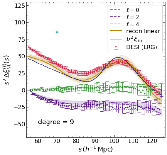
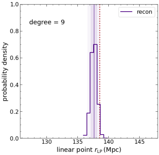
Figure 4: Similar to Fig. 2, showing results for the mock DESI LRG data (Table 1) for $s^{2}\Delta\xi_{\rm NL}^{(\ell)}(s)$ with $\ell=0,2,4$, along with $\Sigma_{\rm obs}^{2}$, analysed with a degree 9 Laguerre function.

The choice of a degree 7 polynomial needs some discussion, since the linear Gaussian analysis of the monopole $\xi_{\rm NL}^{(0)}$ by PS22, using fixed values of $b$, $\beta$ and $\sigma_{\rm v}$, indicated that degree 3 should be sufficient for the BOSS DR12 LRG sample. Our analysis, on the other hand, includes the $\ell=2$ data and allows $\{b,\beta,\sigma_{\rm v}\}$ to vary. We have checked that, using degree 3, 5 and 9 polynomials leads to poorer constraints on $r_{\rm LP}$ ($1\sigma$ errors of $\sim 9.5$ Mpc, $\sim 2.5$ Mpc and $\sim 1.9$ Mpc, respectively) as compared to degree 7 ($\sim 1.6$ Mpc, see above). This indicates that the inclusion of $\ell=2$, along with the opening up of the parameter directions $b$, $\beta$ and $\sigma_{\rm v}$, forces us towards higher degree polynomials, with an optimal degree that leads to the minimum error on $r_{\rm LP}$. We have also checked that including $\ell=4$ measurements in the analysis also degrades the constraints on $r_{\rm LP}$, by broadening the $68\%$ ($95\%$) confidence region by a factor $\sim 2.3\,(1.5)$. This shows that the hexadecapole in BOSS DR12 is expected to add mainly noise rather than signal to the data set (c.f., Ross et al., 2015).

Fig. 4 is formatted identically to Fig. 2 and shows the results of the analysis with the mock DESI LRG measurements of multipoles $\ell=0,2$ and $4$, now with a degree 9 Laguerre function, the choice of degree being made similarly to that described above for the BOSS DR12 mock data. Fig. 5 shows the corresponding a posteriori distributions, with Table 2 summarising the best-fit values of $\{b,\beta,\sigma_{\rm v},\bar{Q}^{(4)}_{4}\}$ and the best fit $\chi^{2}$ per degree of freedom. The degeneracy between $b$ and $\sigma_{\rm v}$ is now more pronounced, largely driven by the reduced error on $\hat{\Sigma}_{\rm obs}^{2}$. The $1\sigma$ uncertainty on $b$ is again $\sim 10\%$ by choice of prior, with the constraint being unbiased relative to the input value. The best-fit and median values of $\sigma_{\rm v}$ agree well with the input value, and the $\sim 10\%$ uncertainty is the same as for the BOSS DR12 mock sample. The $\sim 16\%$ uncertainty on $\beta$ is substantially smaller than for BOSS DR12, but the distribution of $\beta$ excludes the input value at $\gtrsim 99\%$ confidence. Alongside, the best fit values of many of the eigen-coefficients $\mathbf{e}$ are also significantly far from the linear Gaussian expectation at fixed $b$, $\beta$ and $\sigma_{\rm v}$, although each is well-constrained. This is connected to the behaviour of the $\beta$ constraints we highlighted above for the BOSS DR12 mock analysis, and we discuss it further in section 5.2. The auxiliary parameter $\bar{Q}^{(4)}_{4}$ (which has a non-negative prior) is reasonably well-constrained, but with a long positive tail. Finally, the linear point $r_{\rm LP}$ (right panel of Fig. 4) is recovered with very high precision and reasonable accuracy: the median and central $68\%$ confidence interval are $r_{\rm LP}=137.7^{+0.5}_{-0.5}$ Mpc, i.e, a $0.4\%$ uncertainty, with the input value being inside the $95\%$ confidence region.

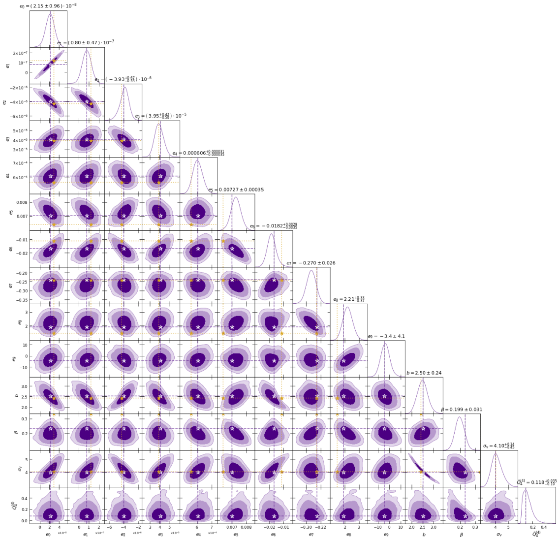
Figure 5: Similar to Fig. 3, for the mock DESI LRG data shown in Fig. 4. In this case, an additional parameter $\bar{Q}^{(4)}_{4}$ was varied in the MCMC analysis (see sections 3.1 and 5.1).

5.2 Theoretical uncertainties and possible improvements

In this section, we discuss some of the limitations of the approximations made in our model and briefly indicate some directions for improvement.

5.2.1 Prior on linear bias

Our results above used a $10\%$ Gaussian prior on the linear bias $b$, which requires some discussion. As mentioned previously, $b$ appears explicitly in our parametrisation only in the evaluation of $\sigma_{\rm eff}^{(\ell)}$ (equations 27), whose dependence on $b$ through explicit factors of $f$ is quite weak, and in the model for $\Sigma_{\rm obs}^{2}$ (equation 47), where $b$ is highly degenerate with $\sigma_{\rm v}$ and also, to some extent, with $\beta$. (The degeneracy with $\sigma_{\rm v}$ is closely connected to the well-known degeneracy between $b$ and $\sigma_{8}$ in usual cosmological analyses of 2pcf observations.)

It is therefore important to ask how our results would be affected if we did not include a strong prior on $b$. For the BOSS DR12 configuration, we have checked that opening up the prior on $b$ to the range $b\in[-20,+20]$ (instead of a $10\%$ Gaussian prior), leads to overall weaker constraints on all parameters which are still unbiased at $95\%$ confidence relative to the input values, with the uncertainties on $b$, $\beta$ and $\sigma_{\rm v}$ being, respectively, $\sim 37\%$, $\sim 40\%$ and $\sim 42\%$. The uncertainties on the eigen-coefficients are typically a factor $2$ larger than those seen in Fig. 3. The corresponding uncertainty on $r_{\rm LP}$, however, is again $\sim 1\%$.

In other words, the main effect of opening up the parameter space along $b$ is to degrade the constraint on $b$ itself and on $\sigma_{\rm v}$ (as expected from their degeneracy), but not on $\beta$ or the linear point. Having said this, we also expect that the combination of galaxy positions and weak gravitational lensing from upcoming surveys should be able to constrain the linear bias to an accuracy of $\sim 10\%$, by breaking the degeneracy between $b$ and $\sigma_{8}$ in those observations (Miyatake et al., 2022; Pandey et al., 2022). In this case, a $10\%$ Gaussian prior on $b$ would not be unrealistic.

We therefore conclude that our choice of prior on $b$ is not likely to be a cause for concern in our framework.

5.2.2 Constraint on $\beta$

As we discussed in section 2.2, we expect our model to become increasingly inaccurate with increasing $\ell$, for sufficiently precise observations (right panel of Fig. 1). This is particularly clear from the behaviour of the constraint on $\beta$ in the DESI LRG configuration presented in section 5.1. For each $\ell$, $\beta$ appears in the model for $\Delta\xi_{\rm NL}^{(\ell)}$ primarily through a multiplicative factor of $\chi_{\ell}(\beta)$ (equations 42-44). Since $\chi_{0}=1+\mathcal{O}(\beta)$, $\chi_{2}=\mathcal{O}(\beta)$ and $\chi_{4}=\mathcal{O}(\beta^{2})$, it is immediately obvious that $\beta$ constraints using high-precision measurements of $\ell=2$ and especially $\ell=4$ will be increasingly sensitive to systematic errors in the model. For example, we have checked that the relative observational errors expected for the DESI LRG $\xi_{\rm NL}^{(4)}(s)$ are smaller than the relative systematic errors in the model (c.f., Fig. 1) by a factor $\gtrsim 2$ for $s\lesssim 90h^{-1}{\rm Mpc}$. Consistently with this, we find that excluding the $\ell=4$ data from the DESI LRG mock analysis leads to unbiased constraints on $\beta$ (although the linear point now shifts to slightly smaller values, excluding the input value at $>95\%$).

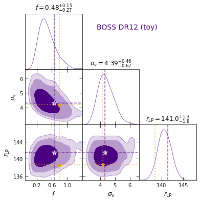
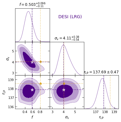
Figure 6: Cosmological constraints from the Laguerre reconstruction exercise for the mock BOSS DR12 (left panel) and DESI LRG data (right panel). These are alternate versions of the constraints shown in Figs. 2-5, focusing on the parameters $\{f,\sigma_{\rm v},r_{\rm LP}\}$, formatted identically to Figs. 3 and 5. The bias in recovering $f$ using the mock DESI LRG data in the right panel is discussed in detail in section 5.2.

5.2.3 Approximation in equation (47)

In equation (46), we introduced an ad hoc factor of $1.38$ to correct the overestimate of $\Sigma_{\rm obs}^{2}$ by our simple model. The value of this factor very likely depends on the parameters $\{b,\beta,\sigma_{\rm v}\}$, although this dependence is probably weak, as seen from the comparison between the DESI LRG and BOSS DR12 configurations above equation (46). However, the error on the measured value of $\hat{\Sigma}_{\rm obs}^{2}$ is only $\sim(1h^{-1}{\rm Mpc})^{2}$ for the DESI LRGs, which is much smaller than the difference $10.9^{2}-9.3^{2}\approx 33(h^{-1}{\rm Mpc})^{2}$ between the model prediction without and with the factor. It is possible, therefore, that the MCMC results are sensitive to the precise value of this factor.

To assess the impact of this approximation, we have repeated the MCMC analysis of the DESI LRG mock data by excluding the measurement of $\Sigma_{\rm obs}^{2}$. We find that the a posteriori distribution of $\beta$ is broader ($\beta=0.220^{+0.044}_{-0.044}$), but has a similar absolute offset of $\sim 0.1$ between its median and the input value $\beta=0.334$ as obtained when including $\Sigma_{\rm obs}^{2}$. The distribution of $\sigma_{\rm v}$, however, now becomes highly biased ($\sigma_{\rm v}=1.79^{+0.54}_{-0.54}\,h^{-1}{\rm Mpc}$), excluding the input value of $\sigma_{\rm v}=4.01\,h^{-1}{\rm Mpc}$ at $>99\%$ confidence. The linear point is unaffected, on the other hand, with a constraint $r_{\rm LP}=138.0^{+0.4}_{-0.4}\,{\rm Mpc}$, which is statistically consistent with the result when including $\Sigma_{\rm obs}^{2}$ and has a similar uncertainty of $\sim 0.3\%$.

This indicates that the inclusion of $\Sigma_{\rm obs}^{2}$ along with the approximation in equation (47) actually helps the model perform better with respect to recovering $\sigma_{\rm v}$, while not affecting the constraint on $r_{\rm LP}$. Improving the smearing approximation in equations (29)-(31) is therefore currently more important than modelling the possible parameter dependence of the normalising factor in equation (47).

5.2.4 Towards a more accurate model

Our mocks treat equation (16) as the truth, so the biases in inferred parameters we found arise from the fact that our Zel’dovich smearing approximation is inadequate for describing DESI LRG-like samples, even in this simple case for which differences between model and truth are as small as those shown in the top right hand panel of Fig. 1. What do we learn from this?

The main deficiency of our model is that its treatment of $\mathcal{O}(K^{4})$ terms and higher is only approximate. In principle, we could extend our treatment by organising the higher order corrections as combinations of powers of $K^{2}$ (i.e., Laplacians in configuration space) and exponentials $\sim{\rm e}^{-K^{2}\sigma^{2}}$ (i.e., Gaussian smoothing kernels) for appropriately chosen smoothing scales $\sigma$. However, in the top left panel of Fig. 1, the zero crossing of $P_{2}$ is at $k<0.2h\,{\rm Mpc}^{-1}$, while in the simulations of Grieb et al. (2016) this does not happen before $k=0.25h\,{\rm Mpc}^{-1}$ (see their fig. 3). Since their choices of redshift, bias and cosmological model are not very different from ours, this discrepancy almost certainly indicates that mode coupling and/or scale-dependent bias – which are absent from our mocks – matter around $k\sim 0.2h\,{\rm Mpc}^{-1}$. Indeed, fig. 2 of Desjacques & Sheth (2010) shows that scale-dependent (density and velocity) bias leave imprints on $\xi_{\rm NL}^{(\ell)}{}$, on BAO scales, that are similar in magnitude to the differences between the solid and dashed curves in Fig. 1.

This suggests that, instead of trying to model equation (16) exactly, we should focus on accounting for mode-coupling and scale-dependent bias. Fortunately, both effects contribute with $k^{2}$ at leading order, so a ‘Laplace-Gaussian’ expansion of the Laguerre-reconstruction approach should be useful, not so much for mimicking equation (16), but for including these other effects as well. We are currently exploring this and will present the results in a forthcoming publication.

5.3 Implications for cosmological inference

The approach presented above has some interesting implications for cosmological inference in general, which we briefly discuss here.

5.3.1 Cosmological constraints

Fig. 6 shows the joint constraints on the set of cosmological parameters $\{f,\sigma_{\rm v},r_{\rm LP}\}$ from the two mock data sets. The model recovers the input values of $\sigma_{\rm v}$ and $r_{\rm LP}$ accurately and precisely for both configurations, and also $f$ for the BOSS DR12 mock. The DESI LRG constraints are biased relative to the input value of the growth rate $f$, for the reasons discussed in section 5.2. Assuming that the Zel’dovich smearing approximation and Laguerre reconstruction scheme can be improved to an accuracy that removes this bias, such a plot can be used to directly compare with any cosmological model that predicts the values of these parameters, not only the $\Lambda$CDM model used here. For example, it would be interesting to explore the region of parameter space covered by linear theory in this plot, when $\Lambda$CDM parameters such as $\{\Omega_{\rm m},h,\sigma_{8}\}$ are varied. This could, in principle, offer a new, model-independent approach to testing dark energy models and/or modified gravity theories.

5.3.2 Choice of tracers

In the context of extracting unbiased constraints on $\beta$, it is worth comparing our approach to that of Hamilton (1992). In that analysis, one completely ignores the smearing due to non-linear growth to find

$$\xi_{\rm NL}^{(2)}/[\xi_{\rm NL}^{(0)}-{\bar{\xi}}^{(0)}_{\rm NL}]=\chi_{2}(\beta)/\chi_{0}(\beta)\,,$$ (61)

where the overbar refers to the volume average in equation (68). In the same approximation, one can also show

$$\xi_{\rm NL}^{(4)}/[\xi_{\rm NL}^{(2)}-(7/5){\bar{\bar{\xi}}}^{(2)}_{\rm NL}]=\chi_{4}(\beta)/\chi_{2}(\beta)\,,$$ (62)

and

$$\xi_{\rm NL}^{(4)}/[\xi_{\rm NL}^{(0)}-{\bar{\xi}}^{(0)}_{\rm NL}+(7/2)({\bar{\xi}}^{(0)}_{\rm NL}-{\bar{\bar{\xi}}}^{(0)}_{\rm NL})]=\chi_{4}(\beta)/\chi_{0}(\beta)\,,$$ (63)

where the double overbar is the volume average in equation (69). Each of these relations could, in principle, be used to extract $\beta$ directly from the observed multipoles of the 2pcf. The MCMC analysis described earlier would then implement this extraction in a fully Bayesian framework.

In our (more realistic) smearing approximation, this simplicity is lost due to the appearance of different smearing scales $\sigma_{\rm eff}^{(\ell)}$ in equations (29)-(31). Equation (27) shows, however, that the differences between the $\sigma_{\rm eff}^{(\ell)}$ could be reduced by considering tracers with either large positive $\beta$, or $\beta<0$. In such cases, equations (29)-(31) can approximately obey Hamilton’s relations, potentially leading to substantial gains in cosmological parameter recovery when combined with constraints on $b$ from lensing studies. Galaxies in voids (having $b\sim 0$ or $b<0$; see, e.g., Paranjape et al., 2018) are likely to be ideal candidates for realising such samples, and could complement existing efforts to include void statistics in parameter recovery (Nadathur et al., 2020, 2022).

Along similar lines, cross-correlating differently biased galaxy sub-samples could also help in parameter recovery, since the corresponding $\sigma_{\rm eff}^{(\ell)}$ and $b_{\rm eff}^{(\ell)}$ values would differ only due to different $b$ values, while having the same values for the cosmological parameters $f$ and $\sigma_{\rm v}$. Such samples would additionally be aided by reduced cosmic variance due to sharing a common volume (McDonald & Seljak, 2009; Wang & Zhao, 2020).

6 Summary & Conclusion

We have charted a path towards using the observed, anisotropic, large-scale 2-point correlation function (2pcf) of galaxies in redshift space to extract cosmological information without relying on a fiducial cosmological model. Such a programme is of particular relevance for testing generic cosmological models, both within general relativity and beyond. Our framework assumes that non-linear growth leads to a smearing of the BAO feature by an approximately Gaussian kernel, and relies on the ‘Laguerre reconstruction’ of the baryon acoustic oscillation (BAO) feature – especially its linear point $r_{\rm LP}$ (Anselmi et al., 2016) – introduced by Nikakhtar et al. (2021a). We have substantially extended the Laguerre reconstruction framework so as to simultaneously model the redshift space multipoles $\xi_{\rm NL}^{(\ell)}(s)$ of the observed 2pcf of biased tracers, for $\ell=0,2,4$.

The starting point of our framework is the Zel’dovich smearing approximation discussed in section 2. We showed that, in the range $55\lesssim s/(h^{-1}{\rm Mpc})\lesssim 125$, all three multipoles under this approximation can be reduced to the isotropic Gaussian smearing of the linear theory real space 2pcf, but with a smoothing scale $\sigma_{\rm eff}^{(\ell)}$ that depends on $\ell$ (equation 27). The accuracy of this approximation is sufficient for use with existing data sets such as the BOSS DR12 LRG sample, but is expected not to be accurate enough for upcoming samples such as DESI LRGs (sections 2.2 and 5.2).

The Laguerre reconstruction scheme in real space relies on a polynomial approximation for the linear theory 2pcf (equation 32), which becomes an expansion in generalised Laguerre functions after a Gaussian smearing (Nikakhtar et al., 2021a, b, 2022). In the approximation mentioned above, this feature extends to all the redshift space multipoles $\xi_{\rm NL}^{(\ell)}$ for $\ell=0,2,4$ (section 3). While this result was already noticed for the monopole $\ell=0$ by Nikakhtar et al. (2021b) and used by those authors as well as Paranjape & Sheth (2022, PS22), our extension of the same ideas to $\ell=2$ and $4$ has significant consequences for parameter recovery. Namely, since the same polynomial coefficients appear in the description of all three multipoles, the additional dependence of these observables on the linear bias $b$, the modified growth rate $\beta=f/b$ and the linear theory velocity dispersion $\sigma_{\rm v}$ can be leveraged to constrain these parameters from observations of the $\xi_{\rm NL}^{(\ell)}$. We emphasize that, unlike standard cosmological BAO analyses (e.g., Anderson et al., 2014; Cuesta et al., 2016; Gil-Marín et al., 2020), as well as recent work on using the linear point for cosmological inference (He et al., 2023), our approach does not assume a fiducial cosmology to model the shape of the BAO feature in redshift space, instead relying on an agnostic basis of functions (here, polynomials).

We tested our framework using mock observations that mimic the existing BOSS DR12 LRG and expected DESI LRG samples (see Table 1). The construction of the mock observations and our MCMC analysis setup are described in section 4, with results presented in section 5. As anticipated, the reconstruction works well for the BOSS DR12 LRG configuration, with unbiased results for the cosmological parameters $\beta$, $\sigma_{\rm v}$ and the linear point $r_{\rm LP}$. For the DESI LRG configuration, while the recovery of $\sigma_{\rm v}$ and $r_{\rm LP}$ remains unbiased, the constraint on $\beta$ excludes the ‘true’ input value at $>99\%$ confidence. The reason for this failure is closely connected to the breakdown of the smearing approximation mentioned above, and is discussed in section 5.2. We also commented in that section on some ways forward in improving the approximation, as well as the role of a reasonably tight prior on the value of $b$, which should be achievable using cross-correlations of the galaxy sample with weak gravitational lensing observations.

Finally, we have not exploited the fact that several of the eigen-coefficients describing the real space linear theory 2pcf $\xi_{\rm lin}(r)$ are statistically consistent with zero in the a posteriori distributions of both the mock samples we studied (Figs. 3 and 5). This fact, which would allow us to substantially decrease the parameter space by only focusing on the most important principle components in the space of polynomial coefficients, can already be determined in the initial, linear Gaussian step of the analysis. It should thus be straightforward to include a step where we only retain these components in the MCMC analysis. Intuitively, these surviving components are likely to be associated with odd, rather than even, Laguerre functions (see, e.g., the discussion in Nikakhtar et al., 2021a). We will test and incorporate this idea, which should further decrease the uncertainties in the recovered parameters, in our future applications.

Our results, and the discussion above, show that it is feasible to extract meaningful constraints on the cosmological parameters $\{f,\sigma_{\rm v},r_{\rm LP}\}$ from upcoming surveys (Fig. 6), without explicitly assuming an underlying cosmological model such as $\Lambda$CDM, and that the sensitivity of this approach can be enhanced by careful choices of sample selection (section 5.3). This bodes well for comparison exercises with a wider class of cosmological models, such as those incorporating dark energy or departures from general relativity. A key requirement for such an exercise would be the prediction of parameters equivalent to $\{f,\sigma_{\rm v},r_{\rm LP}\}$ in these alternate cosmological models. We will expand on this theme in future work.

Data availability

The MCMC chains produced in this work will be made available upon reasonable request to the authors.

Appendix A

A.1 Details of the Zel’dovich smearing approximation

Here we provide some details of the manipulations involved in deriving the final expressions (29)-(31) for the Zel’dovich smearing approximation to equation (16) for $\xi_{\rm NL}^{(\ell)}$.

We use the differential Bessel identity (see 10.1.24 of Abramowitz & Stegun, 1972)

$$j_{\ell}(x)=(-1)^{\ell}\,x^{\ell}\,\left(\frac{1}{x}\frac{{\rm d}}{{\rm d}x}\right)^{\ell}\,j_{0}(x)\,,;\quad\ell=1,2,\ldots\,,$$ (64)

and the Fourier association $\nabla^{2}\leftrightarrow-k^{2}$ to write (16) as

$$\xi_{\rm NL}^{(\ell)}(s) =b_{\rm eff}^{(\ell)2}\,i^{\ell}\,s^{\ell}\left(\frac{1}{s}\frac{\partial}{\partial s}\right)^{\ell}(-\nabla^{-2})^{\ell/2}\,\xi_{0}(s|\sigma_{\rm eff}^{(\ell)})\,,$$ (65)

where we defined $\xi_{0}(s|\sigma)$ in equation (28).

The integro-derivative operator acting on $\xi_{0}(s|\sigma_{\rm eff}^{(\ell)})$ can be simplified for $\ell=2$ and $4$ along the lines of Hamilton (1992). First, note that the 3-dimensional inverse Laplacian of any spherically symmetric function $\xi(s)$ is (Binney & Tremaine, 1987, section 2.4)

$$\nabla^{-2}\xi(s)=-\frac{1}{s}\int_{0}^{s}\,{\rm d}u\,u^{2}\,\xi(u)-\int_{s}^{\infty}{\rm d}u\,u\,\xi(u)\,.$$ (66)

Applying the inverse Laplacian once more and exchanging the order of the resulting double integral gives, after some straightforward algebra,

$$\nabla^{-4}\xi(s) =-\frac{1}{6s}\int_{0}^{s}{\rm d}u\,u^{4}\,\xi(u)-\frac{s}{2}\int_{0}^{s}{\rm d}u\,u^{2}\,\xi(u)$$

$$\phantom{\frac{1}{6}\int{\rm d}u}-\frac{1}{2}\int_{s}^{\infty}{\rm d}u\,u^{3}\,\xi(u)-\frac{s^{2}}{6}\int_{s}^{\infty}{\rm d}u\,u\,\xi(u)\,.$$ (67)

Finally, define the volume averages $\bar{\xi}(s)$ and $\bar{\bar{\xi}}(s)$ of any function $\xi(s)$ as

$$\bar{\xi}(s) \equiv\frac{3}{s^{3}}\int_{0}^{s}{\rm d}u\,u^{2}\,\xi(u)\,,$$ (68)

$$\bar{\bar{\xi}}(s) \equiv\frac{5}{s^{5}}\int_{0}^{s}{\rm d}u\,u^{4}\,\xi(u)\,,$$ (69)

Repeated differentiation of $\nabla^{-\ell}\xi_{0}(s|\sigma_{\rm eff}^{(\ell)})$ for $\ell=0,2$ and $4$ then gives us equations (29)-(30).

The following identities are useful for the numerical evaluation of the approximation shown in the right panel of Fig. 1,

$$\xi_{0}(s|\sigma) =\int{\rm d}\ln k\,\Delta_{\rm lin}^{2}(k)\,{\rm e}^{-k^{2}\sigma^{2}/2}\,j_{0}(ks)\,,$$

$$\bar{\xi}_{0}(s|\sigma) =\int{\rm d}\ln k\,\Delta_{\rm lin}^{2}(k)\,{\rm e}^{-k^{2}\sigma^{2}/2}\,3j_{1}(ks)/(ks)\,,$$

$$\bar{\bar{\xi}}_{0}(s|\sigma) =\int{\rm d}\ln k\,\Delta_{\rm lin}^{2}(k)\,{\rm e}^{-k^{2}\sigma^{2}/2}\,\frac{5}{(ks)^{3}}\bigg{[}2\sin(ks)$$

$$\phantom{\int{\rm d}\ln k\,\Delta_{\rm lin}^{2}(k)\,{\rm e}^{-k^{2}}}+\left((ks)^{2}-6\right)j_{1}(ks)\bigg{]}\,.$$ (70)

A.2 Gauss-Poisson covariance matrix

Here, we discuss some implications of the Gauss-Poisson approximation (49) for the covariance of 2pcf measurements that are relevant for understanding the magnitude of errors on measurements of multipoles with increasing $\ell$. In the following, we focus on Fourier space and denote $\mu_{k}\equiv\hat{n}\cdot\hat{k}$ as $\mu$ for brevity.

As discussed in the main text, at BAO scales, the smearing approximation for the non-linear power spectrum works well. We can then write the anisotropic power spectrum as

$$P(k,\mu)\approx b^{2}\,(1+\beta\mu^{2})^{2}\,P_{\rm lin}(k)\,{\rm e}^{-k^{2}\sigma_{\rm v}^{2}(1-\mu^{2})}{\rm e}^{-k^{2}\sigma_{\rm v}^{2}\mu^{2}(1+f)^{2}},$$ (71)

for which the integral over $\mu$ which defines $\sigma^{2}_{\ell_{1}\ell_{2}}$ in equation (50) can be done analytically for all $(\ell_{1},\ell_{2})$. This is because the integral over $\mu$ is simplified by noting that if

$${\cal I}_{j}(\kappa)\equiv\int_{-1}^{1}\frac{d\mu}{2}\,{\rm e}^{-\kappa^{2}\mu^{2}/2}\,\mu^{j},$$ (72)

then

$$\kappa^{2}\,{\cal I}_{2(n+1)}(\kappa)=(2n+1)\,{\cal I}_{2n}(\kappa)-{\rm e}^{-\kappa^{2}/2},$$ (73)

with

$${\cal I}_{0}(\kappa)=\frac{\sqrt{\pi}}{2}\,\frac{{\rm erf}(\kappa/\sqrt{2})}{\kappa/\sqrt{2}}.$$ (74)

(Note that all ${\cal I}_{2n+1}(\kappa)=0$.) The multipoles $P_{0}$ and $P_{2}$ of $P(k,\mu)$ are then

$$P_{0}(k)=b^{2}\,P_{\rm lin}(k)\,{\rm e}^{-k^{2}\sigma_{\rm v}^{2}}\sum_{j=0}^{2}{2\choose j}\beta^{j}\,{\cal I}_{2j}(K),$$ (75)

and

$$\frac{P_{2}(k)}{5}=b^{2}\,P_{\rm lin}(k)\,{\rm e}^{-k^{2}\sigma_{\rm v}^{2}}\sum_{j=0}^{2}{2\choose j}\beta^{j}\,\left[\frac{3{\cal I}_{2j+2}(K)-{\cal I}_{2j}(K)}{2}\right]\,,$$ (76)

and $\sigma_{00}^{2}$ becomes

$$\frac{\sigma^{2}_{00}}{2V_{\rm sur}/({\bar{n}}V_{\rm sur})^{2}} =1+2\,{\bar{n}}P_{0}(k)$$

$$+b^{4}\,{\bar{n}}^{2}P^{2}_{\rm lin}(k)\,{\rm e}^{-2k^{2}\sigma_{\rm v}^{2}}\sum_{j=0}^{4}{4\choose j}\,\beta^{j}\,{\cal I}_{2j}(\sqrt{2}K)$$ (77)

where $K^{2}=2k^{2}\sigma_{\rm v}^{2}f(2+f)$. The other $\ell_{1}\ell_{2}$ pairs simply involve more powers of $\mu^{2}$, so yield other combinations of the ${\cal I}_{2j}$.

This leaves the integral over $k$ as the only one which must be done numerically, since only the shot-noise piece is analytic:

$$\int\frac{dk\,k^{2}}{2\pi^{2}}\,\bar{j}_{\ell_{1}}(ks_{i})\,\bar{j}_{\ell_{2}}(ks_{j})$$

$$=\frac{(4\pi)^{2}}{V_{i}V_{j}}\int ds\,s^{2}\,W_{i}(s)\int dt\,t^{2}\,W_{j}(t)\int\frac{dk\,k^{2}}{2\pi^{2}}\,j_{\ell_{1}}(ks)\,j_{\ell_{2}}(kt)\,$$

$$=\frac{4\pi}{V_{i}V_{j}}\int ds\,s^{2}\,W_{i}(s)\,W_{j}(s)\,.$$ (78)

For non-overlapping tophat bins of unit height, the integral is zero unless $i=j$, in which case the expression above becomes $1/V_{i}$. I.e., this shotnoise term contributes as $\delta_{ij}\,2\,(V_{\rm sur}/V_{i})/({\bar{n}}V_{\rm sur})^{2}$, where we recognize that ${\bar{n}}V_{\rm sur}=N$, so $2\,(V_{\rm sur}/V_{i})/N^{2}\approx(V_{i}/V_{\rm sur})^{-1}/{N\choose 2}$. This diverges in the limit of small bins, as expected. For typical BAO samples which have ${\bar{n}}P\sim 1$ at $k\sim 0.1\,h\,{\rm Mpc}^{-1}$, the other terms dominate unless the bins are substantially narrower than a tenth of an Mpc.

However, to gain intuition, it is useful to invoke the smearing approximation and write the anisotropic power spectrum as

$$P(k,\mu)\approx\sum_{\ell}P_{\ell}(k)\,\mathcal{P}_{\ell}(\mu)$$ (79)

with

$$P_{\ell}(k)\equiv P_{\rm lin}(k)\,b_{\rm eff}^{(\ell)2}\,{\rm e}^{-k^{2}\sigma_{\rm eff}^{(\ell)2}/2}\,,$$ (80)

where $b_{\rm eff}^{(\ell)}$ and $\sigma_{\rm eff}^{(\ell)}$ were defined in equations (26) and (27), respectively. Then, the orthogonality of Legendre polynomials means that the $1/\bar{n}^{2}$ term in equation (50) gives $\delta_{\ell_{1}\ell_{2}}\,(2\ell_{1}+1)\,2/(\bar{n}^{2}V_{\rm sur})$. The term proportional to $(2P(k,\mu)/\bar{n}V_{\rm sur})$ involves the product of three Legendre polynomials, which equation (4) simplifies to

$$\frac{2}{\bar{n}V_{\rm sur}}\,(2\ell_{1}+1)(2\ell_{2}+1)\,2\sum_{\ell}\begin{pmatrix}\ell_{1}&\ell_{2}&\ell\\ 0&0&0\end{pmatrix}^{2}\,P_{\ell}(k)\,.$$ (81)

Finally, the term proportional to $P^{2}(k,\mu)$ involves four Legendre polynomials. It can be simplified by using the fact that

$$\mathcal{P}_{\ell_{1}}(\mu)\,\mathcal{P}_{\ell_{2}}(\mu)=\sum_{\ell=|\ell_{1}-\ell_{2}|}^{\ell_{1}+\ell_{2}}\begin{pmatrix}\ell_{1}&\ell_{2}&\ell\\ 0&0&0\end{pmatrix}^{2}(2\ell+1)\,\mathcal{P}_{\ell}(\mu);$$ (82)

this reduces the expression to the product of three polynomials, and then equation (4) further simplifies it to

$$\frac{2}{V_{\rm sur}} \,(2\ell_{1}+1)(2\ell_{2}+1)\sum_{\ell=|\ell_{1}-\ell_{2}|}^{\ell_{1}+\ell_{2}}\begin{pmatrix}\ell_{1}&\ell_{2}&\ell\\ 0&0&0\end{pmatrix}^{2}\,(2\ell+1)$$

$$\times\sum_{\ell^{\prime}}\sum_{\ell^{\prime\prime}}\begin{pmatrix}\ell&\ell^{\prime}&\ell^{\prime\prime}\\ 0&0&0\end{pmatrix}^{2}P_{\ell^{\prime}}(k)\,P_{\ell^{\prime\prime}}(k).$$ (83)

When $\ell_{1}=\ell_{2}=0$ (for the covariance of the monopole) then this term becomes

$$\frac{2}{V_{\rm sur}}\,\sum_{\ell^{\prime}}\sum_{\ell^{\prime\prime}}\begin{pmatrix}0&\ell^{\prime}&\ell^{\prime\prime}\\ 0&0&0\end{pmatrix}^{2}P_{\ell^{\prime}}(k)\,P_{\ell^{\prime\prime}}(k)=\frac{2}{V_{\rm sur}}\,\sum_{\ell}\frac{P_{\ell}^{2}(k)}{2\ell+1},$$ (84)

making

$$\sigma^{2}_{00}(k) =\frac{2}{V_{\rm sur}}\,\sum_{\ell}\frac{P_{\ell}^{2}(k)}{2\ell+1}+\frac{2}{\bar{n}V_{\rm sur}}\,2P_{0}(k)+\frac{2}{\bar{n}^{2}V_{\rm sur}}$$

$$=\frac{2}{V_{\rm sur}}\,\left[\left(P_{0}(k)+\frac{1}{\bar{n}}\right)^{2}+\sum_{\ell>0}\frac{P_{\ell}^{2}(k)}{2\ell+1}\right].$$ (85)

Notice that this has a contribution from the higher order multipoles, in addition to the naive term one might expect from the monopole itself. Similarly,

$$\sigma^{2}_{22}(k) =\frac{2}{V_{\rm sur}}\times 5\,\bigg{[}\left(P_{0}(k)+\frac{1}{\bar{n}}\right)^{2}+\frac{3}{7}\,P^{2}_{2}(k)$$

$$\phantom{2}+\frac{1789}{9009}\,P_{4}^{2}(k)+\frac{4}{7}\left(P_{0}(k)+\frac{1}{\bar{n}}\right)[P_{2}(k)+P_{4}(k)]$$

$$\phantom{2V_{\rm sur}}+\frac{24}{77}P_{2}(k)P_{4}(k)\bigg{]}$$ (86)

and

$$\sigma^{2}_{44}(k) =\frac{2}{V_{\rm sur}}\times 9\,\bigg{[}\left(P_{0}(k)+\frac{1}{\bar{n}}\right)^{2}+\frac{1789}{5005}\,P^{2}_{2}(k)$$

$$\phantom{2}+\frac{529}{1001}\frac{9}{17}\,P_{4}^{2}(k)+\frac{360}{1001}P_{2}(k)P_{4}(k)$$

$$\phantom{2}+\left(P_{0}(k)+\frac{1}{\bar{n}}\right)\left(\frac{40}{77}P_{2}(k)+\frac{324}{1001}P_{4}(k)\right)\bigg{]}.$$ (87)

The cross terms are

$$\sigma^{2}_{02}(k) =\frac{2}{V_{\rm sur}}\bigg{[}\,2\left(P_{0}(k)+\frac{1}{\bar{n}}\right)\,P_{2}(k)$$

$$+\frac{2}{7}\left(P^{2}_{2}(k)+2P_{2}(k)P_{4}(k)+\frac{50}{99}P^{2}_{4}(k)\right)\bigg{]}\,,$$ (88)

$$\sigma^{2}_{04}(k) =\frac{2}{V_{\rm sur}}\bigg{[}2\left(P_{0}(k)+\frac{1}{\bar{n}}\right)\,P_{4}(k)$$

$$+\frac{2}{7}\left(\frac{9}{5}P^{2}_{2}(k)+\frac{81}{143}P^{2}_{4}(k)+\frac{20}{11}P_{2}(k)\,P_{4}(k)\right)\bigg{]}$$ (89)

and

$$\sigma^{2}_{24}(k) =\frac{2}{V_{\rm sur}}\bigg{[}2P_{2}(k)P_{4}(k)$$

$$\phantom{2/Vs}+\frac{2}{7}\left(P_{0}(k)+\frac{1}{\bar{n}}\right)\left(18P_{2}(k)+\frac{100}{11}P_{4}(k)\right)$$

$$+\frac{2}{7}\left(\frac{54}{11}P^{2}_{2}(k)+\frac{450}{143}P^{2}_{4}(k)+\frac{788}{143}P_{2}(k)P_{4}(k)\right)\bigg{]}.$$ (90)

For most galaxy samples $P_{0}(k)>P_{2}(k)>P_{4}(k)$ around BAO scales $k\sim 0.1\,h\,{\rm Mpc}^{-1}$ (see, e.g., the left panel of Fig. 1, or fig. 3 of Grieb et al., 2016), which suggests that

$$\sigma^{2}_{\ell\ell}(k)\approx(2\ell+1)\,\sigma^{2}_{00}(k)$$ (91)

should be reasonably accurate. Indeed, this expression mimics the dependence on $\ell$ shown in fig. 4 of Grieb et al. (2016) quite well. Similarly,

$$\sigma^{2}_{0\ell}(k)\approx\frac{2}{V_{\rm sur}}\,2\left[P_{0}(k)+\frac{1}{\bar{n}}\right]\,P_{\ell}(k).$$ (92)

In this case,

$$R_{\ell_{1}\ell_{2}}(k)\equiv\frac{\sigma^{2}_{\ell_{1}\ell_{2}}(k)}{\sigma_{\ell_{1}\ell_{1}}(k)\sigma_{\ell_{2}\ell_{2}}(k)}\approx\frac{\sigma^{2}_{\ell_{1}\ell_{2}}(k)/\sigma^{2}_{00}(k)}{\sqrt{(2\ell_{1}+1)(2\ell_{2}+1)}}.$$ (93)

making

$$R_{0\ell}(k)\approx\frac{\sigma^{2}_{0\ell}(k)/\sigma^{2}_{00}(k)}{\sqrt{(2\ell+1)}}=\frac{2}{\sqrt{2\ell+1}}\frac{\bar{n}P_{\ell}(k)}{\bar{n}P_{0}(k)+1}.$$ (94)

This seems to be in good agreement with the $k_{i}=k_{j}$ (diagonal) elements shown in fig. 5 of Grieb et al. (2016).

References

- Abbott et al. (2022) Abbott T. M. C., et al., 2022, Phys. Rev. D, 105, 043512
- Abramowitz & Stegun (1972) Abramowitz M., Stegun I. A., 1972, Handbook of Mathematical Functions. Dover Publications Inc., New York
- Alam et al. (2015) Alam S., et al., 2015, ApJS, 219, 12
- Alam et al. (2017) Alam S., et al., 2017, MNRAS, 470, 2617
- Anderson et al. (2012) Anderson L., et al., 2012, MNRAS, 427, 3435
- Anderson et al. (2014) Anderson L., et al., 2014, MNRAS, 439, 83
- Anselmi et al. (2016) Anselmi S., Starkman G. D., Sheth R. K., 2016, MNRAS, 455, 2474
- Anselmi et al. (2018a) Anselmi S., Corasaniti P.-S., Starkman G. D., Sheth R. K., Zehavi I., 2018a, Phys. Rev. D, 98, 023527
- Anselmi et al. (2018b) Anselmi S., Starkman G. D., Corasaniti P.-S., Sheth R. K., Zehavi I., 2018b, Phys. Rev. Lett., 121, 021302
- Beutler et al. (2014) Beutler F., et al., 2014, MNRAS, 443, 1065
- Beutler et al. (2017) Beutler F., et al., 2017, MNRAS, 466, 2242
- Bharadwaj (1996) Bharadwaj S., 1996, ApJ, 472, 1
- Binney & Tremaine (1987) Binney J., Tremaine S., 1987, Galactic dynamics. Princeton University Press, Princeton, NJ
- Blas et al. (2011) Blas D., Lesgourgues J., Tram T., 2011, J. Cosmology Astropart. Phys, 2011, 034
- Blomqvist et al. (2019) Blomqvist M., et al., 2019, , 629, A86
- Chuang et al. (2015) Chuang C.-H., Kitaura F.-S., Prada F., Zhao C., Yepes G., 2015, MNRAS, 446, 2621
- Cole et al. (2005) Cole S., et al., 2005, MNRAS, 362, 505
- Crocce & Scoccimarro (2006) Crocce M., Scoccimarro R., 2006, Phys. Rev. D, 73, 063520
- Crocce & Scoccimarro (2008) Crocce M., Scoccimarro R., 2008, Phys. Rev. D, 77, 023533
- Cuesta et al. (2016) Cuesta A. J., et al., 2016, MNRAS, 457, 1770
- DESI Collaboration et al. (2016) DESI Collaboration et al., 2016, arXiv e-prints, p. arXiv:1611.00036
- Desjacques & Sheth (2010) Desjacques V., Sheth R. K., 2010, Phys. Rev. D, 81, 023526
- Eisenstein et al. (2005) Eisenstein D. J., et al., 2005, ApJ, 633, 560
- Eisenstein et al. (2007) Eisenstein D. J., Seo H.-J., Sirko E., Spergel D. N., 2007, ApJ, 664, 675
- Gil-Marín et al. (2020) Gil-Marín H., et al., 2020, MNRAS, 498, 2492
- Grieb et al. (2016) Grieb J. N., Sánchez A. G., Salazar-Albornoz S., Dalla Vecchia C., 2016, MNRAS, 457, 1577
- Hamilton (1992) Hamilton A. J. S., 1992, ApJ, 385, L5
- He et al. (2023) He M., Zhao C., Shan H., 2023, arXiv e-prints, p. arXiv:2303.10661
- Hunter (2007) Hunter J. D., 2007, Computing In Science & Engineering, 9, 90
- Kaiser (1987) Kaiser N., 1987, MNRAS, 227, 1
- Lesgourgues (2011) Lesgourgues J., 2011, arXiv e-prints, p. arXiv:1104.2932
- Lewis (2019) Lewis A., 2019, arXiv e-prints, p. arXiv:1910.13970
- Marra & Chirinos Isidro (2019) Marra V., Chirinos Isidro E. G., 2019, MNRAS, 487, 3419
- McDonald & Seljak (2009) McDonald P., Seljak U., 2009, J. Cosmology Astropart. Phys, 2009, 007
- Menote & Marra (2022) Menote R., Marra V., 2022, MNRAS, 513, 1600
- Miyatake et al. (2022) Miyatake H., et al., 2022, Phys. Rev. D, 106, 083520
- Nadathur et al. (2020) Nadathur S., et al., 2020, MNRAS, 499, 4140
- Nadathur et al. (2022) Nadathur S., et al., 2022, MNRAS, 516, 2936
- Nikakhtar et al. (2021a) Nikakhtar F., Sheth R. K., Zehavi I., 2021a, Phys. Rev. D, 104, 043530
- Nikakhtar et al. (2021b) Nikakhtar F., Sheth R. K., Zehavi I., 2021b, Phys. Rev. D, 104, 063504
- Nikakhtar et al. (2022) Nikakhtar F., Sheth R. K., Zehavi I., 2022, Phys. Rev. D, 105, 043536
- Noda et al. (2020) Noda E., Peloso M., Pietroni M., 2020, Physics of the Dark Universe, 29, 100579
- Nunes et al. (2020) Nunes R. C., Yadav S. K., Jesus J. F., Bernui A., 2020, MNRAS, 497, 2133
- Padmanabhan et al. (2012) Padmanabhan N., Xu X., Eisenstein D. J., Scalzo R., Cuesta A. J., Mehta K. T., Kazin E., 2012, MNRAS, 427, 2132
- Pandey et al. (2022) Pandey S., et al., 2022, Phys. Rev. D, 106, 043520
- Paranjape & Sheth (2022) Paranjape A., Sheth R. K., 2022, MNRAS, 517, 4696
- Paranjape et al. (2018) Paranjape A., Hahn O., Sheth R. K., 2018, MNRAS, 476, 3631
- Peloso et al. (2015) Peloso M., Pietroni M., Viel M., Villaescusa-Navarro F., 2015, J. Cosmology Astropart. Phys, 2015, 001
- Ross et al. (2015) Ross A. J., Percival W. J., Manera M., 2015, MNRAS, 451, 1331
- Sánchez et al. (2011) Sánchez E., et al., 2011, MNRAS, 411, 277
- Taylor & Hamilton (1996) Taylor A. N., Hamilton A. J. S., 1996, MNRAS, 282, 767
- Torrado & Lewis (2019) Torrado J., Lewis A., 2019, Cobaya: Bayesian analysis in cosmology, Astrophysics Source Code Library, record ascl:1910.019 (ascl:1910.019)
- Torrado & Lewis (2021) Torrado J., Lewis A., 2021, J. Cosmology Astropart. Phys, 2021, 057
- Van Der Walt et al. (2011) Van Der Walt S., Colbert S. C., Varoquaux G., 2011, preprint, (arXiv:1102.1523)
- Virtanen et al. (2020) Virtanen P., et al., 2020, Nature Methods, 17, 261
- Wang & Zhao (2020) Wang Y., Zhao G.-B., 2020, Research in Astronomy and Astrophysics, 20, 158
- Wigner (1993) Wigner E. P., 1993, On the Matrices Which Reduce the Kronecker Products of Representations of S. R. Groups. Springer Berlin Heidelberg, Berlin, Heidelberg, pp 608–654, doi:10.1007/978-3-662-02781-3˙42, https://doi.org/10.1007/978-3-662-02781-3_42
- Zel’dovich (1970) Zel’dovich Y. B., 1970, 5, 84
- Zhao et al. (2021) Zhao C., et al., 2021, MNRAS, 503, 1149
- Zhou et al. (2020) Zhou R., et al., 2020, Research Notes of the American Astronomical Society, 4, 181
- du Mas des Bourboux et al. (2020) du Mas des Bourboux H., et al., 2020, ApJ, 901, 153