ALR-GAN: Adaptive Layout Refinement for Text-to-Image Synthesis

Abstract

We propose a novel Text-to-Image Generation Network, Adaptive Layout Refinement Generative Adversarial Network (ALR-GAN), to adaptively refine the layout of synthesized images without any auxiliary information. The ALR-GAN includes an Adaptive Layout Refinement (ALR) module and a Layout Visual Refinement (LVR) loss. The ALR module aligns the layout structure (which refers to locations of objects and background) of a synthesized image with that of its corresponding real image. In ALR module, we proposed an Adaptive Layout Refinement (ALR) loss to balance the matching of hard and easy features, for more efficient layout structure matching. Based on the refined layout structure, the LVR loss further refines the visual representation within the layout area. Experimental results on two widely-used datasets show that ALR-GAN performs competitively at the Text-to-Image generation task.

I Introduction

Text-to-Image Generation (T2I) aims to synthesize photorealistic images from a text description. To realize this challenging cross-modal generation task can facilitate multimedia tasks such as image editing [48, 22], story visualization [17], and cross-modal retrieval [6]. Owing to Generative Adversarial Networks (GANs) [5], the latest T2I methods facilitate the synthesis of high-resolution images [47, 8, 49], refinement of image details [43, 52, 14, 15], and enhancement of image semantics [35, 26, 44, 25, 45].

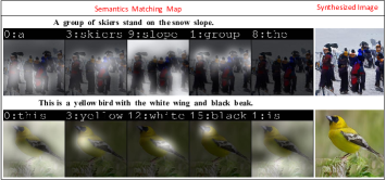
Figure 1: Visualization of semantics-matching maps and corresponding synthesized image. The brighter the color, the more semantic correlation between the word and image subregions.

While these T2I methods can synthesize high-quality images, they tend to focus on single-object synthesis, such as a bird, flower, or dog. For complex image synthesis tasks such as those on the MS-COCO dataset [21], synthesized objects are easily placed on various unreasonable locations of the image, i.e., the layout structure (which refers to the locations of the objects and background) is chaotic. Some excellent methods [13, 19, 11, 16] have improved the layout structure through auxiliary information such as the object bounding box, object shape, and scene graph. However, 1) the acquisition of this auxiliary information is generally expensive and not conducive to the promotion and application of the task; and 2) these methods generally ignore the visual quality within the layout area. We aim to improve the layout of the synthesized image with no auxiliary information.

We exploit the layout structure information from the image and text description to improve the layout structure of the synthesized image. In the Text-to-Image matching task [3, 7, 51], each word has semantics-matched subregions on its corresponding image by matching semantics between words and image subregions. In Fig. 1, highlighted areas indicate the semantic correlation between the word and corresponding image subregions, reflecting the semantic location or structure information of the word on the image. Accordingly, all semantics-matched subregions of words in the text description reflect the layout structure of the corresponding image. Therefore, the obvious idea is to align the layout structure of the synthesized image with that of its corresponding real image based on semantics-matching. However, in the layout structure matching process, the structures of some subregions are easier to align than others. Such hard subregions cause major difficulty in layout refinement. Thus, in each training stage, the model should spend more effort in layout structure matching in such hard subregions. For this, we design an adaptive weight adjustment mechanism to adaptively improve the hard and easy structures for the synthesized image.

In addition to improving the layout structure, we enhance the visual representation of the synthesized image. One of the most straightforward ideas is to directly constrain the visual consistency between the whole synthesized image and the whole real image. However, the semantics of the text description only covers some partial semantics of the images in general. Over-constraint on layout and details that are not included in the text description can significantly increase the training burden of the model. Thus, within the corrected layout area, we try to align the visual representations of the synthesized and corresponding real images.

Finally, we propose an Adaptive Layout Refinement Generative Adversarial Network (ALR-GAN) to improve the layout of the synthesized image. The ALR-GAN includes an Adaptive Layout Refinement (ALR) module and Layout Visual Refinement (LVR) loss. The ALR module and the proposed Adaptive Layout Refinement (ALR) loss act to adaptively align the layout structure of the synthesized image with the visual representation of its corresponding real image. The adaptive weight adjustment mechanism in the ALR loss adaptively balances the matching weights of hard and easy parts in the layout structure alignment process. In the layout refined by the ALR module, the LVR loss is designed to align the texture perception and style information of the synthesized image with that of its corresponding real image. Our contributions can be summarized as follows:

$\bullet$ We propose an ALR module, equipped with the proposed ALR loss to adaptively refine the layout structure of synthesized images.

$\bullet$ We propose LVR loss to enhance the visual representation within the layout.

$\bullet$ Experimental results and analysis show the efficacy of ALR-GAN on the CUB-Bird [41] and large-scale MS-COCO [21] benchmarks based on four metrics.

II Related Work

In current T2I models, the design and refinement of layouts of synthesized objects and details are often achieved with the help of auxiliary information. Visual Question Answering (VQA) datasets are used to enhance object semantics during image synthesis [4, 30, 24, 10]. These models extract semantic information from questions and feed it to the VQA model. Visual question-answering loss is adopted to align the semantics in generated images with those extracted in the VQA tasks. Another type of auxiliary information, the object box [33, 32, 31, 50], helps control the structure of objects in synthesized scenes. The object box defines the location of each object using a bounding box with a category label. It can be used to control the placement of these objects during image synthesis from a higher-level perspective. Object shape information is another type of auxiliary information that has been used [12, 16] to help generator networks improve the geometric properties of synthesized objects. In text description, the relationship between multiple objects can often be more explicitly represented using a more structured scene graph. Compared with the plain text description, scene graphs can encode more information on objects’ positions and spatial relationships, which can provide explicit guidance in layout design and refinement  [13, 40, 18].

While auxiliary information can effectively help the layout design, it must be obtained through extra data collection and annotation procedures (which are often expensive and not scalable) or by solving additional tasks (which might not be easier than T2I itself). Unlike the above, we exploit layout structure information from the text description and corresponding images. Layout design and refinement can then be performed together with the mainstream T2I pipelines, without collecting extra auxiliary information.

III Adaptive Layout Refinement Generative Adversarial Network

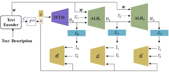
Figure 2: Architecture of proposed ALR-GAN.

Fig. 2 shows the architecture of the proposed ALR-GAN, which contains two new components: the Adaptive Layout Refinement (ALR) module and Layout Visual Refinement (LVR) loss. The ALR module is equipped with the proposed Adaptive Layout Refinement (ALR) loss to adaptively refine the layout structure of a synthesized image with the aid of that of its corresponding real image. LVR loss aims to enhance the texture perception and style information within the layout area.

We provide an overview of the ALR-GAN structure in section III-A, describe the ALR module in section III-B, describe the LVR loss in section III-C, and summarize all the losses for ALR-GAN in section III-D.

III-A Overview

As shown in Fig. 2, ALR-GAN contains a text encoder [43]; a conditioning augmentation module [47] $F^{ca}$; $m$ generators $G_{i}$, $\emph{i}=0,1,2,\ldots,m-1$); an Initial Feature Transition Module (IFTM); $m-1$ ALR modules $ALR_{i}$, $\emph{i}=1,2,\ldots,m-1$; and $m$ discriminators $D_{i}$, $\emph{i}=0,1,2,\ldots,m-1$.

The text encoder transforms the input text description (a single sentence) into a sentence feature $s^{\prime}$ and word features $W$. $F^{ca}$ [47] converts $s^{\prime}$ to a conditioning sentence feature $s$. The IFTM translates the text embedding $s$ and noise $z\sim N(0,1)$ into the image feature $H_{0}$, which is an initial generation stage. The ALR module adaptively refines the layout structure of synthesized images in the training process. In the training stage, the input information of $ALR_{i}$ consists of the word features $W$, image feature $H_{i-1}$, and $i^{th}$ scale real image $I_{i}^{*}$. The ouput information of $ALR_{i}$ is the image feature $H_{i}$. In the testing stage, $ALR_{i}$ takes the image feature $H_{i-1}$ and word feature $W$ to produce the hidden feature $H_{i}$. Note that during the testing stage, the input information to the generator does not include real images.

III-B Adaptive Layout Refinement module

Without the aid of auxiliary information, we need to exploit the layout structure information from text and images, and refine the layout structure of the synthesized image. As described in section I, we can obtain the layout structure information of the image from the semantics-matching between words and image subregions. To this end, we can align the layout structure of the synthesized image with that of its corresponding real image. To achieve this goal, we propose the Adaptive Layout Refinement (ALR) module, whose architecture is shown in Fig. 3.

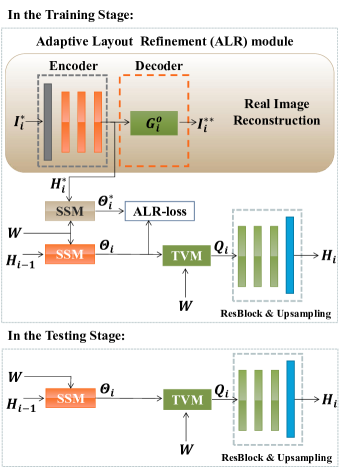
Figure 3: Architecture of ALR module in training and testing stage. SSM: Semantics Similarity Matrix; ALR loss: Adaptive Layout Refinement loss; TVM: Text-Vision Matrix. In the ResBlock & Upsampling part, the green box is the ResBlock module, and the Upsampling module is blue. In the training stage, the ALR module requires the participation of real images, which provide the high-quality layout information for the generator; in the testing stage, the input information of the ALR module does not include the real image.

III-B1 Construction of Layout Structure

In the $i^{th}$ ALR_i module, the word embeddings are denoted as $W=\{w_{j}\in\mathbb{R}^{D}|j=1,2,\cdots,T\}$, the image feature of the previous stage $ALR_{i-1}$ or IFTM is denoted as $H_{i-1}=\{h^{k}_{i-1}\in\mathbb{R}^{D}|k=1,2,\cdots,N=W_{H}\times H_{H}\}$, $N$ is the number of image subregions ($W_{H}$ and $H_{H}$ are the respective width and height of feature $H_{i-1}$), $D$ is the dimension of the feature, and $T$ is the number of words.

We capture the layout structure from the semantics matching between the words $W$ and image subregions $H_{i-1}$, defined as

$$\theta_{k,j}=\frac{exp(S_{k,j}^{\prime})}{\sum_{k=1}^{T}exp(S_{k,j}^{\prime})},\,\,\,\,S^{\prime}_{k,j}=(h^{k}_{i-1})^{T}w_{j}.$$ (1)

Here $\Theta=\{\theta_{k,j}|k=1,2,\cdots,N;j=1,2,\cdots,T\}$ is called a Semantics Similarity Matrix (SSM), $\theta_{k,j}$ is the semantics similaity weight between the ${j}^{th}$ word $w_{i}$ and the $k^{th}$ image subregion $h^{k}_{i-1}$, and the above calculation process is defined as a function, $\Theta_{i-1}=SSM(W,H_{i-1})$. Without ambiguity, we omit the subscripts $i-1$ of $\Theta$, i.e., $\Theta=SSM(W,H_{i-1})$.

In $\Theta$, each matrix $\Theta_{j}\in\mathbb{R}^{W_{H}\times H_{H}}$ calculates the semantics similarity between the ${j}^{th}$ word $w_{j}$ and all image subregions $H$. When the weight $\Theta_{j}$ is overlaid on the image, as shown in Fig. 1, the highlighted visual regions express that their semantics are related to the word $w_{j}$. Accordingly, $\Theta$ encodes the layout structure of the image. However, the layout structure of the synthesized image is often chaotic due to incorrect or inadequate understanding of text semantics by the generator. Thus, we hope that $\Theta$ of the synthesized image is aligned with that of the real image. Before alignment, we need to calculate $\Theta^{*}$ of the real image $I^{*}_{i}$.

As shown in Fig. 3, we use the encoder (which contains a series of convolution blocks) to extract feature $H^{*}_{i}$ of the real image $I^{*}_{i}$. To ensure the quality of $H^{*}_{i}$, we put $H^{*}_{i}$ in $G_{i}(\cdot)$ to reconstruct image $I^{**}_{i}$, and introduce the reconstruction loss,

$$\mathcal{L}^{REC}_{i}=||I^{*}_{i}-I^{**}_{i}||_{1}$$ (2)

Then $\Theta^{*}$ of the real image $I^{*}_{i}$ is calculated by $\Theta^{*}=SSM(W,H^{*}_{i})$.

III-B2 Adaptive Layout Refinement (ALR) loss

We can align $\Theta$ with $\Theta^{*}$ by minimizing $||\Theta-\Theta*||_{F}$. During optimization, some elements in $\Theta$ and $\Theta^{*}$ are easy to match, and some are hard. A hard region causes major problems in the layout refinement process. Thus, during training, the model should pay more attention to matching in hard regions. Balancing easy versus hard information is important to improve the model’s performance [23, 20, 2]. We propose Adaptive Layout Refinement (ALR) loss to address this issue. There are four steps to its construction.

Step 1. Calculate the absolute residual tensor $R=Abs.(\Theta^{*}-\Theta)$, $R=\{r_{i,j}|i=1,2,\cdots,N;j=1,2,\cdots,T\}$, where “Abs” denotes the absolute operation.

Step 2. Divide the elements in $R$ into hard and easy parts. We set a threshold value $\gamma$. Elements $r_{i,j}<\gamma$ are easy to match, and elements $r_{i,j}\geq\gamma$ are hard to match.

Step 3. Define the adaptive weight adjustment terms for the easy and hard parts. Recently,  [23, 20, 2, 42] adaptively adjusted the loss weights for hard and easy samples, but these adjustments are suitable for the sample but not the feature pixel. Thus, we design an adaptive feature-level weight adaptation mechanism to adjust loss weights for easy and hard matching elements in $\Theta$ and $\Theta^{*}$. There are four steps (3.a-3.d) to construct the adaptive weight adaptation mechanism. We show the adaptive weight adjustment mechanism for the easy part, and the adjustment for the hard part is similar.

Step 3.a. Keep the elements of $R$ less than $\gamma$, set the rest to $0$, and call it a tensor, $R^{\prime}_{easy}$.

Step 3.b. $R^{\prime}_{easy}\in\mathbb{R}^{N\times T}$ is maped into the same latent space as $H^{*}$ by padding with zeros, which is called $R_{easy}$.

Step 3.c. The feature corresponding to the easy part $R_{easy}$ on real image feature $H^{*}$ is calculated by $R_{easy}\odot H^{*}$.

Step 3.d. The loss weight of $R_{easy}$ is denoted as $\alpha$, which is learned from $\alpha=\phi_{\alpha}(R_{easy}\odot H^{*})$. Here, $\phi_{\alpha}(\cdot)$ is composed of a series of neural layers and activation layers, and $\odot$ denotes the Hadamar Product. Note that $\alpha$ has the same dimension as $R$.

For the hard part, we keep the elements of $R$ larger than $\gamma$, set the rest to $0$, and call it $R_{hard}$. The loss weight of $R_{hard}$ is denoted as $\beta$, and this is learned from $\beta=\phi_{\beta}(R_{hard}\odot H^{*})$. $\phi_{\beta}(\cdot)$ is also composed of a series of neural and activation layers.

Step 4. In the training process, the hard part should be better focused on. Therefore, the weight $\beta$ should be bigger than $\alpha$. So, we design a regularization item $softplus(\max(\alpha)-\min(\beta))$ in $L_{ALR}$ to satisfy it. Here, $y=softplus(x)=\ln(1+e^{x})$ is a monotonically increasing function that helps numerical optimization by avoiding negative loss values.

Based on Steps 1–4, the ALR loss is defined by

$$L^{ALR}_{i}=\frac{1}{N\cdot D}(||\alpha_{i}\odot R_{easy_{i}}||_{F}+||\beta_{i}\odot R_{hard_{i}}||_{F}$$ (3)

$$+||softplus(\max(\alpha_{i})-\min(\beta_{i}))||_{F})$$

where the subscript $F$ stands for frobenius norm, and $\gamma=0.2$ is based on experiments on a hold-out validation set.

III-B3 Constructing the Text-vision Matrix (TVM)

Based on the corrected SSM $\Theta$, for the $k^{th}$ subregion, the dynamic representation of words w.r.t. $h^{k}_{i-1}$ is $q^{k}_{i-1}=\sum_{j=1}^{T}\theta_{j,k}w_{j}$. So, the Text-Vision Matrix (TVM) for word embeddings $W$ and image feature $H_{i-1}$ is denoted by $Q_{i-1}=(q^{1}_{i-1},q^{2}_{i-1},...,q^{N}_{i-1})\in\mathbb{R}^{D\times N}$. The TVM $Q_{i-1}$ and image feature $H_{i-1}$ are concatenated, and fed into the ResBlocks and Upsampling modules to output the image feature $H_{i}$.

III-C Layout Visual Refinement (LVR) loss

Based on the refined layout structure, we further enhance the visual representation within the layout area. To do this, we propose Layout Visual Refinement (LVR) loss to enhance the texture perception and style information in the layout. LVR loss includes Perception Refinement (PR) loss and Style Refinement (SR) loss.

III-C1 Perception Refinement loss

To contruct Perception Refinement (PR) loss, we first construct the layout mask. In SSM $\Theta\in\mathbb{R}^{T\times N}$, each column consists of the semantics similarity weights between one subregion and all words. The maximum value in each column is the most related word to the subregion. Therefore, we use a maximization operation in each column of $\Theta(^{*})$ to get $Mask_{\Theta(^{*})}\in\mathbb{R}^{W_{H}\times H_{H}}$. Then we capture the image feature within the layout: the layout masks $Mask_{\Theta}$ and $Mask_{\Theta*}$ dot product the $H_{i}$ and $H^{*}_{i}$, respectively. Finally, the perception refinement loss is defined as

$$L^{PR}_{i}=\frac{1}{N\cdot D}\|Mask_{\Theta_{i}}\odot H_{i}-Mask_{\Theta^{*}_{i}}\odot H^{*}_{i}\|_{F}$$ (4)

$L_{PR_{i}}$ can drive the generator to better enhance the texture perception in the layout area.

III-C2 Style Refinement loss

To further enhance style-related information in the layout, we align the Gram Matrix of the $Mask_{\Theta_{i}}\odot H_{i}$ with that of the $Mask_{\Theta^{*}_{i}}\odot H^{*}_{i}$, and define the Style Refinement (SR) loss as

$$~{}L^{SR}_{i}=\frac{1}{N\cdot D}\|\mathcal{G}(Mask_{\Theta_{i}}\odot H_{i})-\mathcal{G}(Mask_{\Theta^{*}_{i}}\odot H^{*}_{i})\|_{F}$$ (5)

where $\mathcal{G}(\cdot)$ is Gram Matrix calculation.

The LVR Loss is defined as $L^{LVR}_{i}=\eta_{1}\mathcal{L}^{PR}_{i}+\eta_{2}\mathcal{L}^{SR}_{i}$. The hyperparameters $\eta_{1}=1.0$ and $\eta_{2}=1.0$ are based on experiments on a holdout validation set.

III-D Objective Functions in ALR-GAN

Combining the above modules, at the $i$-th stage of ALR-GAN, the generative loss $\mathcal{L}_{G_{i}}$ is defined as

$$L_{G_{i}}=\underbrace{-\frac{1}{2}\mathbb{E}_{\hat{I_{i}}\sim P_{G_{i}}}[logD_{i}(\hat{I_{i}})]}_{\text{unconditional loss}}-\underbrace{\frac{1}{2}\mathbb{E}_{\hat{I_{i}}\sim P_{G_{i}}}[logD_{i}(\hat{I_{i}},s)]}_{\text{conditional loss}},$$ (6)

where the unconditional loss pushes the synthesized image to be more realistic, to fool the discriminator, and the conditional loss drives the synthesized image to better match the corresponding text description. The discriminative loss is defined as

$$L_{D_{i}}= \underbrace{-\frac{1}{2}\mathbb{E}_{I^{*}_{i}\sim P_{data_{i}}}[logD_{i}(I^{*}_{i})]-\frac{1}{2}\mathbb{E}_{\hat{I_{i}}\sim P_{G_{i}}}[log(1-D_{i}(\hat{I_{i}})]}_{\text{unconditional loss}}+$$ (7)

$$\underbrace{-\frac{1}{2}\mathbb{E}_{I^{*}_{i}\sim P_{data_{i}}}[logD_{i}(I^{*}_{i},s)]-\frac{1}{2}\mathbb{E}_{\hat{I_{i}}\sim P_{G_{i}}}[log(1-D_{i}(\hat{I_{i}},s)]}_{\text{conditional loss}},$$

where $I^{*}_{i}$ and $\hat{I_{i}}$ are the $i$-th scale image, the discriminative loss $\mathcal{L}_{D_{i}}$ classifys the input image sampling from the real image distribution or synthesized image distribution.

To generate realistic images, the final objective functions of the generative and discriminative networks are defined respectively as

$$L_{G}=\sum_{i=0}^{m-1}L_{G_{i}}+\sum_{i=1}^{m-1}[L^{ALR}_{i}+\lambda_{1}L^{REC}_{i}+L^{LVR}_{i}]+\lambda_{2}L_{DAMSM},$$ (8)

$$L_{D}=\sum_{i=0}^{m-1}L_{D_{i}}.$$ (9)

Here, ALR-GAN has three stage generators ($m=3$), and $\lambda_{1}=10^{-1}$. The parameter $\lambda_{2}=50$ in the MS-COCO dataset, and the parameter $\lambda_{2}=5$ in the CUB-Bird dataset. The values of $\lambda_{2}$ in ALR-GAN are the same as in AttnGAN [43] and DM-GAN [52]. The parameter $\lambda_{2}$ is used to balance the loss $\mathcal{L}_{DAMSM}$ in the generative loss $L_{G}$, and is introduced to improve the semantics-matching between image subregions and words.

TABLE I: IS $\uparrow$, FID $\downarrow$, SOA-C/SOA-I $\uparrow$, and R-Precision $\uparrow$ by some SOTA GAN-based T2I models and ALR-GAN on the CUB-Bird and MS-COCO test sets. W A.I.: With Auxiliary Information. W/O A.I.: Without Auxiliary Information. Scores for models marked with * were calculated with pretrained models provided by the respective authors. First, second, and third scores are shown in red, green, and blue, respectively.

Pattern	Method	CUB-Bird			MS-COCO
		IS	FID	R-Presion (%)	IS	FID	R-Presion (%)	SOA-C	SOA-I
	Obj-GAN [16]	-	-	-	$30.29\pm 0.33$	$25.64$	$91.05$	$27.14^{*}$	$41.24^{*}$
W A.I.	OP+AttnGAN [11]	-	-	-	$27.88\pm 0.12$	$24.70$	$89.01$	$35.85$	$50.47$
	CP-GAN [19]	-	-	-	$52.73\pm 0.61$	-	$93.59$	$77.02$	$84.55$
	RiFe-GAN [1]	$5.23\pm 0.09$	-	$\sim 22.5$(Average)	$31.70$	-	-	-
	AttnGAN [43]	$4.36\pm 0.02$	$23.98$	$52.62^{*}$	$25.89\pm 0.19$	$35.49$	$61.34^{*}$	$25.88^{*}$	$39.01^{*}$
	CSM-GAN [37]	$4.62\pm 0.08$	$20.18$	$54.92^{*}$	$26.77\pm 0.24$	$33.48$	$63.84^{*}$	$27.24^{*}$	$42.10^{*}$
	SE-GAN [35]	$4.67\pm 0.04$	$18.17$	-	$27.86\pm 0.31$	$32.28$	-	-	-
	DM-GAN [52]	$4.75\pm 0.07$	$16.09$	$59.21^{*}$	$30.49\pm 0.57$	$32.64$	$70.63^{*}$	$33.44^{*}$	$48.03^{*}$
W/O A.I.	KT-GAN [36]	$4.85\pm 0.04$	$17.32$	$70.76^{*}$	$31.67\pm 0.36$	$30.73$	$65.20^{*}$	$35.02^{*}$	$42.86^{*}$
	DF-GAN [39]	$4.86\pm 0.04$	$19.24$	-	-	-	-	-	-
	DAE-GAN [28]	$4.42\pm 0.04$	$15.19$	$59.44^{*}$	$35.08\pm 1.16$	$28.12$	$73.81^{*}$	$38.41^{*}$	$57.30^{*}$
	DR-GAN [38]	$4.90\pm 0.05$	$14.96$	$61.17^{*}$	$34.59\pm 0.51$	$27.80$	$77.27^{*}$	$41.62^{*}$	$60.73^{*}$
	XMC-GAN [46]	-	-	-	$30.45$	$9.33$	$71.00$	$50.94$	$71.33$
	Baseline	$4.51\pm 0.04$	$23.32$	$71.63$	$29.17\pm 0.22$	$33.67$	$61.29$	$31.74$	$47.12$
	ALR-GAN	4.96 $\pm$ 0.04	$15.14$	$77.54$	$34.70\pm 0.66$	$29.04$	$69.20$	$42.47$	$62.20$
W/O A.I.	DMGAN [52]+ALR+LVR	$4.81\pm 0.06$	$15.37$	$63.90$	$35.27\pm 0.46$	$29.42$	$74.28$	$43.13$	$58.90$
	DAE-GAN [28]+ALR+LVR	$4.53\pm 0.09$	$14.26$	$62.03$	$37.02\pm 0.76$	$23.79$	$79.40$	$55.64$	$72.56$
	DR-GAN [38]+ALR+LVR	$4.94\pm 0.03$	$14.70$	$64.40$	$35.12\pm 0.57$	$26.03$	$79.04$	$49.73$	$73.10$

IV Experimental Results

We discuss the experiment settings, compare ALR-GAN with many GAN-based T2I methods, and evaluate the effectiveness of each component. In the training stage: (i) in the CUB-Bird dataset, the training batch size is $16$, and the training epoch is $800$; (2) in the MS-COCO dataset, the training batch size is $14$, and the training epoch is $150$. All experiments about ALR-GAN are trained and tested on one GTX 3090 GPU respectively.

IV-A Experiment Settings

IV-A1 Datasets

ALR-GAN was evaluated on two public datasets, CUB-Bird [41] and MS-COCO [21]. CUB-Bird contains $11,788$ bird images, and $10$ sentences for each image. MS-COCO contains $80$K training images and $40$K testing images, each with five sentences. The testing and training sets were preprocessed using the same pattern as in [27, 47]. We adopt the image generated by the first sentence in the testing dataset as our “Testing Set”. The data setting is the same as these SOTA T2I methods [52, 28, 38]. Besides, we adopt the image generated by the second sentence in the testing dataset as our “Validation Set”. So, the number of the “Testing set” and “Validation set” in CUB-Bird is $2933$; the number of the “Testing set” and “Validation set” in MS-COCO is $\sim$ $40K$.

IV-A2 Baseline

Our baseline model is AttnGAN [43] with Spectral Normalization [34], which limits drastic gradient changes and improves training efficiency, and hence model performance. Due to GPU memory limitations, the Baseline model includes three generators, each with a corresponding discriminator. The first through third generators generate $64\times 64$, $128\times 128$, and $256\times 256$ images, respectively.

IV-A3 Evaluation

We use four measures to evaluate the performance of ALR-GAN, where $\uparrow$ means that the higher the value the better the performance, and vice versa. Inception Score (IS$\uparrow$):  [29] This is obtained by an Inception-V3 model fine-tuned by [47] to calculate the KL-divergence between the marginal and conditional class distributions. A large IS indicates that synthesized images have high diversity for all classes, and each image can be recognized as a specific class. Fréchet Inception Distance (FID$\downarrow$): [9] A lower FID score between synthesized and real images means that the synthesized image distribution is closer to the real image distribution, and that the generator can synthesize photo-realistic images. Semantic Object Accuracy (SOA$\uparrow$ ): This includes SOA-C and SOA-I scores. SOA-C is the percentage of synthesized images per class in which the desired object is detected, and SOA-I is the percentage of synthesized images in which the desired object is detected. R-precision$\uparrow$: This is used to evaluate the semantic consistency between a synthesized image and the corresponding text description.

IV-B Comparison with state-of-the-art GAN models

Image Diversity and Objective Evaluation. We use IS scores, as shown in Table I, to evaluate the objectives and diversity of synthesized images on the CUB-Bird and MS-COCO test sets. Compared with T2I methods Without Auxiliary Information (W/O A.I. in Table I), ALR-GAN performs competitively. The IS score of DAE-GAN [28] is higher than that of ALR-GAN on the MS-COCO dataset because DAE-GAN uses extra NLTK POS tagging and manually designs rules for different datasets. Compared with T2I methods With Auxiliary Information (W A.I. in Table I), the IS score of RiFe-GAN [1] is higher than that of ALR-GAN on CUB-Bird, and the IS score of CP-GAN [19] is higher than that of ALR-GAN on MS-COCO, because RiFe-GAN [1] requires additional text sentences to train the model. CP-GAN [19] requires additional auxiliary information, including the object’s bounding box and shape, to train the T2I model. In contrast, we only explore the layout information from the image and the text description, without additional auxiliary information, to guide the generator to correct the layout, to synthesize a high-quality image. Here, the DAE-GAN+ALR+LVR and DR-GAN+ALR+LVR are trained on one Tesla V100 GPU from scratch. We adopt the DAE-GAN and DR-GAN pre-trained model released by authors to synthesize images on one GTX 3090 GPU respectively. All experiments about DM-GAN+ALR+LVR are trained and tested on one GTX 3090 GPU. We also train the DM-GAN+ALR+LVR from scratch.

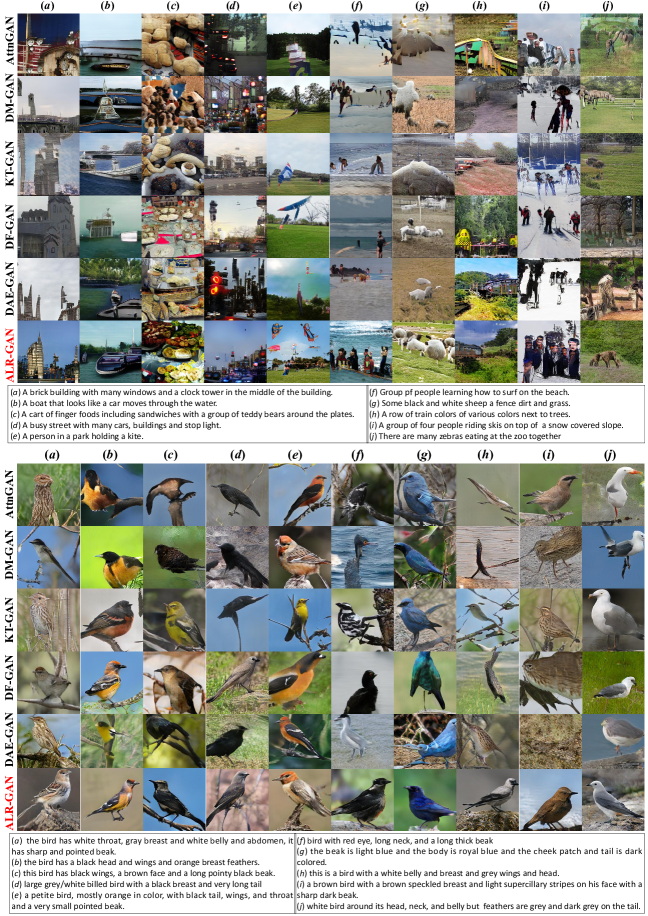
Figure 4: Images of $256\times 256$ resolution are synthesized by AttnGAN, DM-GAN, KT-GAN, DF-GAN, DAE-GAN, and ALR-GAN conditioned on text descriptions from MS-COCO dataset (Upper Part) and CUB-Bird dataset (Lower Part).

Semantic Object Accuracy Evaluation. We adopt the SOA score (which includes the SOA-C and SOA-I scores) [11] to evaluate the quality of individual objects and regions within an image on the MS-COCO dataset. As shown in Table I, the SOA-C and SOA-I scores of ALR-GAN are much better than those of most T2I methods (including DAE-GAN [28]) and Baselines without auxiliary information. ALR-GAN is better than methods with auxiliary information, such as Obj-GAN [16] and OP-GAN [11]. The SOA-C and SOA-I scores of XMC-GAN [46] and CP-GAN [19] are higher than those of ALR-GAN. CP-GAN [19] requires additional auxiliary information, including the object’s bounding box and shape. XMC-GAN adopted contrastive learning to capture inter-modality and intra-modality correspondences, which enriched the global semantics and region semantics of the synthesized image. The intra-modality correspondence can push the synthesized image into the real image. The synthesized image distribution is closer to the real image distribution. The SOA-C is the percentage of synthesized images per class in which the desired object is detected, and SOA-I is the percentage of synthesized images in which the desired object is detected. Sufficient global and regional semantics of synthesized images are conducive to object recognition, so XMC-GAN gets high SOA-I/SOA-C scores.

Distribution and Semantics Consistency Evaluation. We use the FID to evaluate distribution consistency between real and synthesized images. We use the R-precision proposed by AttnGAN [43] to evaluate the semantic consistency between the text description and synthesized image. As shown in Table I, ALR-GAN achieves competitive performance on two measures, and is much better than our Baseline. The FID score of DAE-GAN [28] is higher than that of ALR-GAN because DAE-GAN uses extra NLTK POS tagging and manually-designed rules for different datasets, while we only explore the layout information from the image and the text description, without additional auxiliary information.

Generalization. To observe the generalization of the ALR module and LVR loss, we introduce them into DMGAN [52], DR-GAN [38], and DAE-GAN [28]. As shown in Table I, these two designs can help these methods perform better on different measures because they are designed to refine the layout structure and enhance the visual representation of the object or background within the layout. However, these components intuitively constrain the diversity of layouts. In fact, the layouts of objects in training samples are diverse. Thus, they guide the generator to better learn the distribution of the object’s layout. Therefore, for the same text description, the generator still can synthesize diverse layouts, as shown in Fig. 5. Hence our proposed ALR module and LVR loss are plugin designs that can be applied to other T2I models.

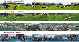
Figure 5: Examples of ALR-GAN on ability to catch subtle changes (phrase or words in red) of text descriptions on MS-COCO test set, and synthesizing diverse images with reasonable layout.

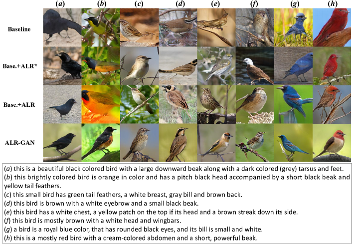
Figure 6: Images ($256\times 256$) synthesized by Baseline (Base.), Base.+ALR, and ALR-GAN conditioned on text descriptions from CUB-Bird test set.

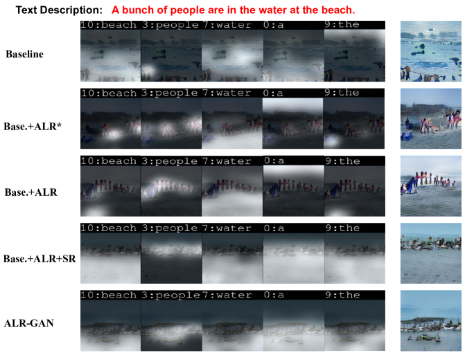
Figure 7: Semantics-matched regions between words and image from Baseline (Base.), Base.+ALR^∗, Base.+ALR, Base.+ALR+PR, and ALR-GAN. Highlighted region is semantics-matched region between word and whole image.

Visualization Evaluation. We qualitatively evaluate ALR-GAN and some outstanding GAN-based T2I methods by image visualization on the CUB-Bird and MS-COCO test sets. On CUB-Bird, the image is dominated by a single bird. Compared with other methods, ALR-GAN can improve the layout and detail semantics of various parts of the bird’s body in the Lower Part of Fig. 4. On MS-COCO, images are usually scene-type images with a variety of objects or backgrounds. Compared with CUB-Bird, there is little specific appearance information of a single object in MS-COCO. Therefore, the visual quality of the synthesized objects in this dataset is not as good as in CUB-Bird. We can observe from the Upper Part of Fig. 4 that the layout quality synthesized by ALR-GAN is more reasonable than by other T2I methods. Although DAE-GAN has a better IS score on COCO than ALR-GAN, the latter focuses on layout generation. On the COCO dataset, the layout synthesized by ALR-GAN is better than by DAE-GAN.

We further evaluate the sensitivity of the proposed ALR-GAN by changing just one word or phrase in the input sentence. As shown in Fig. 5, the synthesized images are modified according to the words or phrase changes of the input text description, e.g., image scene and objects (“in water,” “on a grass field,” “people,” “cows,” “sheep”). We can see that ALR-GAN also can catch subtle changes of the text description and retain semantic diversity from text and reasonable layouts.

Model Cost. Table II compares ALR-GAN with SOTA T2I methods under four model cost measures: Training Time, Training Epoch, Model Size, and Testing Time. Using the MS-COCO dataset as an example, compared with these methods, the model cost of ALR-GAN is appropriate.

TABLE II: Training Time, Training Epochs, Model Size, and Testing Time of ALR-GAN and SOTA T2I methods on MS-COCO dataset.

Method	Training Time	Training Epoch	Model Size	Testing Time
AttnGAN [43]	$\sim 8Days$	$120$	$\sim 55.5M$	$\sim 1200s$
DM-GAN[52]	$\sim 14Days$	$200$	$\sim 89.7M$	$\sim 1800s$
DAE-GAN[28]	$\sim 11Days$	$200$	$\sim 91M$	$\sim 1900s$
DF-GAN[39]	-	$300$	$\sim 189M$	-
DR-GAN[38]	$\sim 10Days$	$150$	$\sim 73.2M$	$\sim 1400s$
ALR-GAN(Ours)	$\sim 10Days$	$150$	$\sim 76M$	$\sim 1400s$

IV-C Ablation Study

We evaluate the effectiveness of the ALR module and LVR loss. The IS score, FID score, SOA-C score, and SOA-I score are shown in Table III. The IS and FID scores produced by combining different components on the CUB-Bird dataset; the SOA-C score and SOA-I score produced by combining different components on the MS-COCO dataset.

We gradually add these components to the Baseline (Base.), and introduce the ALR module, i.e., Base.+ALR. As shown in Table III, compared with the Baseline, on the CUB-Bird dataset, Base.+ALR improves the IS score from $4.51$ to $4.79$, and the FID score of Base.+ALR drops from $23.32$ to $17.33$; on the MS-COCO Dataset, Base.+ALR improves the SOA-C score from $31.74$ to $38.12$, and improves the SOA-I score from $47.12$ to $55.81$. We introduce the Perception Refinement (PR) loss to Base.+ALR, i.e., Base.+ALR+PR. As shown in Table III, compared with Base.+ALR, on the CUB-Bird dataset, Base.+ALR+PR improves the IS score from $4.79$ to $4.84$, and the FID score of Base.+ALR+PR drops from $17.33$ to $16.08$; on the MS-COCO Dataset, Base.+ALR+PR improves the SOA-C score from to $38.12$ to $40.28$, and improves the SOA-I score from $55.81$ to $57.29$. We introduce the LVR loss to Base.+ALR, i.e., ALR-GAN. Compared with Base.+ALR+PR, ALR-GAN improves the performance over four measures. Note that the LVR loss contains the Perception Refinement (PR) and Style Refinement (SR) loss.

TABLE III: IS $\uparrow$ and FID $\downarrow$ produced by combining different components on CUB-Bird dataset. SOA-C $\uparrow$ and SOA-I $\uparrow$ produced by combining different components on MS-COCO dataset.

Method	CUB-Bird		MS-COCO
	IS	FID	SOA-C	SOA-I
Baseline (Base.)	4.51 $\pm$ 0.04	$23.32$	$31.74$	$47.12$
Base.+ALR	4.79$\pm$ 0.03	$17.33$	$38.12$	$55.81$
Base.+ALR+PR	4.84 $\pm$ 0.05	$16.08$	$40.28$	$57.29$
ALR-GAN	4.96 $\pm$ 0.04	$15.14$	$42.47$	$62.20$
Base.+ALR∗	4.58$\pm$ 0.03	$21.03$	$35.85$	$50.11$
Base.+ALR+PR∗	4.81$\pm$ 0.02	$16.92$	$39.65$	$56.31$
Base.+ALR+PR+SR∗	4.86$\pm$ 0.07	$16.13$	$41.63$	$59.44$

We discuss the effectiveness of the adaptive weight adjustment mechanism in $L^{ALR}_{i}$ (Eq. 3). We substitute $\|\Theta-\Theta^{*}\|_{F}$ for $L^{ALR}_{i}$ (Eq. 3) in the ALR module, i.e., Base.+ALR^†, in Table III. Base.+ALR^∗ performs worse than Base.+ALR. As shown in Fig. 6 and Fig. 7, the layout structure of the synthesized image is worse than that of Base.+ALR. This indicates that the adaptive weight adjustment mechanism can effectively improve the matching efficiency between $\Theta$ and $\Theta^{*}$, to further improve image quality.

We discuss the importance of Perception Refinement (PR) loss $L^{PR}_{i}$ (Eq. 4) in LVR loss $L^{LVR}_{i}$. We substitute $\frac{1}{N\cdot D}\|H-H^{*}\|_{F}$ for $L^{PR}_{i}$ (Eq. 4), i.e., Base.+ALR+PR^∗, in Table III. Compared with Base.+ALR+PR, the performance of Base.+ALR+PR^∗ is worse. We further discuss the importance of Style Refinement (SR) loss ($L^{SR}_{i}$, Eq. 5) in LVR loss $L^{LVR}_{i}$. As shown in Fig. 7, from Base.+ALR to Base.+ALR+SR, the style and layout information of the synthesized images is significantly improved. We further substitute $\frac{1}{N\cdot D}\|\mathcal{G}(H)-\mathcal{G}(H^{*})\|_{F}$ for $L^{SR}_{i}$ (Eq. 5), i.e., Base.+ALR+PR+SR^∗, in Table III. Compared with ALR-GAN, the performance of Base.+ALR+PR+SR^∗ is also worse. Through the experimental results, we can simply analyze the reasons. This is because the semantics of the text description only covers part of the semantics of the image. Over-constraint on the layout and details that are not included in the text description can significantly increase the training burden of the model. For the synthesized image, this additional uncontrollable visual information generation will interfere with image quality evaluation.

Finally, we qualitatively evaluate the effectiveness of each component by image visualization (Fig. 6 and Fig. 7). In Fig. 6, we can see that these proposed strategies can effectively improve the details, structure, and layout of birds. And, with the addition of losses, the structure and layout of the birds gradually improves. In Fig. 7, we can also see that with the introduction of modules or loss functions, the attention area and layout structure of the scene, the style information are gradually improved. Overall, these ablation studies indicate that the ALR module and LVR loss can effectively improve the details, structure, and layout of the synthesized images.

IV-D Parametric Sensitivity Analysis

We analyze the sensitivity of $\gamma$, $\eta_{1}$, $\eta_{2}$, $m$, and $\lambda_{1}$.

TABLE IV: IS $\uparrow$ and FID $\downarrow$ of different values of $\gamma$ on CUB-Bird dataset. SOA-C $\uparrow$ and SOA-I $\uparrow$ of different values of $\gamma$ on MS-COCO dataset.

Method	CUB-Bird		MS-COCO
	IS	FID	SOA-C	SOA-I
$\gamma=0,1.0$	$\sim 4.6$	$\sim 20.1$	$\sim 36.4$	$\sim 52.2$
$\gamma=0.1$	4.89$\pm$ 0.04	$16.11$	$41.87$	$58.61$
$\gamma=0.2$	4.96 $\pm$ 0.04	$15.14$	$42.47$	$62.20$
$\gamma=0.3$	4.94 $\pm$ 0.07	$15.59$	$42.65$	$60.22$
$\gamma=0.5$	4.90 $\pm$ 0.04	$15.64$	$42.66$	$59.96$
$\gamma=0.8$	4.83 $\pm$ 0.03	$16.22$	$39.45$	$54.73$

TABLE V: IS $\uparrow$ and FID $\downarrow$ under different numbers of generators on CUB-Bird dataset. SOA-C $\uparrow$ and SOA-I $\uparrow$ are under different numbers of generators on MS-COCO dataset. $m=0,1,2$: number of generators is $1$, $2$, and $3$, respectively.

Method	CUB-Bird		MS-COCO
	IS	FID	SOA-C	SOA-I
$m=0$	2.91 $\pm$ 0.10	$48.22$	$5.27$	$15.03$
$m=1$	4.05 $\pm$ 0.08	$32.17$	$22.53$	$36.74$
$m=2$	4.96 $\pm$ 0.04	$15.14$	$42.47$	$62.20$

TABLE VI: IS $\uparrow$ and FID $\downarrow$ of different values of $\eta_{1}$ on CUB-Bird dataset. SOA-C $\uparrow$ and SOA-I $\uparrow$ of different values of $\eta_{1}$ on MS-COCO dataset.

Method	CUB-Bird		MS-COCO
	IS	FID	SOA-C	SOA-I
$\eta_{1}=0$	4.88$\pm$ 0.07	$16.20$	$40.28$	$58.84$
$\eta_{1}=0.1$	4.93$\pm$ 0.10	$15.08$	$42.21$	$62.84$
$\eta_{1}=0.5$	4.92 $\pm$ 0.09	$15.44$	$41.00$	$62.12$
$\eta_{1}=1.0$	4.96 $\pm$ 0.04	$15.14$	$42.47$	$62.20$
$\eta_{1}=5.0$	4.66 $\pm$ 0.02	$19.45$	$35.22$	$50.63$

TABLE VII: IS $\uparrow$ and FID $\downarrow$ of different values of $\eta_{2}$ on CUB-Bird dataset. SOA-C $\uparrow$ and SOA-I $\uparrow$ of different values of $\eta_{2}$ on MS-COCO dataset.

Method	CUB-Bird		MS-COCO
	IS	FID	SOA-C	SOA-I
$\eta_{2}=0$	4.84$\pm$ 0.05	$16.08$	$40.28$	$57.29$
$\eta_{2}=0.1$	4.90$\pm$ 0.09	$16.05$	$43.70$	$59.01$
$\eta_{2}=0.5$	4.94 $\pm$ 0.04	$15.62$	$41.82$	$61.94$
$\eta_{2}=1.0$	4.96 $\pm$ 0.04	$15.14$	$42.47$	$62.20$
$\eta_{2}=5.0$	4.71 $\pm$ 0.10	$18.33$	$36.62$	$52.67$

Hyperparameter $\gamma$. The threshold value $\gamma$ seperates the easy and hard parts in ALR loss. We set $\gamma$ to different values and observe the performance of ALR-GAN, as reported in Table IV, from which we see that ALG-GAN achieves the best performance when $\gamma=0.2$. When $\gamma=0$ or $\gamma=1.0$, there is no weight balance mechanism for the simple and hard parts, which results in a moderate drop in performance. When $\gamma=0$ or $\gamma=1.0$, the attention weight in the ALR loss is still obtained through model learning. As shown in Table IV, ALG-GAN still maintains appropriate performance.

Hyperparameters $\eta_{1}$ and $\eta_{2}$. The LVR loss includes the Perception Refinement (PR) loss and Style Refinement (SR) loss. Hyperperameters $\eta_{1}$ and $\eta_{2}$ are used to adjust the training weights of the PR and SR loss, respectively. The numerical experimental results of parameter sensitivity are reported in Tables VI and VII. (i) When $\eta_{1}=0$ or $\eta_{2}=0$, the performance of the model degrades; it means that two sub-loss functions in LVR loss can help improve the quality of the synthesized image; (ii) When $\eta_{1}\in[0.1,1.0]$ or $\eta_{2}\in[0.1,1.0]$, the performance of the model is stable. The values of the two parameters in $[0.1,1.0]$ will not cause dramatic changes in model performance; (iii) When the two parameters are too large, the performance is significantly degraded. This is because the goal of the GAN is to learn the real image distribution and generate diverse images. This is a kind of global distribution learning based on local sampling. Although such consistency loss as LVR loss helps to improve the quality of the generated image, if the training weight is too large, the model will fall into the strong constraint of local samples. This destroys the learning mechanism of GANs and is prone to mode collapse.

Hyperparameter $m$. We discuss the effect of the number of generators on the quality of the synthesized image. The results are reported in Table V. The values $m=0,1,2$, respectively, indicate $1$, $2$, and $3$ generators. We can clearly see that the quality of the generated images increases with the number of generators. Due to memory limitations and fair comparison with other SOTA methods, ALR-GAN contains three generators, i.e., $m=2$.

Hyperparameter $\lambda_{1}$. We further show the sensitivity of $\lambda_{1}$, as shown in Table VIII. In ALR-GAN, $\lambda_{1}$ is used to adjust the training weight of the image reconstruction loss $L^{REC}_{i}$ (Eq. 2) in $L_{G}$ (Eq. 8). The goal of the loss function $L^{REC}_{i}$ is to provide high-quality real image features to the ALR mechanism. When $\lambda_{1}=0$, the loss function $L^{REC}_{i}$ is removed, at which point the image encoder can easily lose important visual or layout information. In this way, low-quality real image features will mislead the generator to depict poor-quality layout structure and visual semantics. When $\lambda_{1}=0.001~{}or~{}0.1$, the performance of the model is stable. With the increase of $\lambda_{1}$, the performance of the model decreases. This is similar to model performance when $\eta_{1}$ and $\eta_{2}$ are increased. If the training weight is too large, the model will fall into the strong constraint of local samples. The training center of ALR-GAN is also transferred to the learning of sample consistency, which weakens the GAN’s learning of distribution, destroying its learning mechanism, and making it prone to mode collapse.

TABLE VIII: IS $\uparrow$ and FID $\downarrow$ of different values of hyperparameter $\lambda_{1}$ on CUB-Bird dataset. SOA-C $\uparrow$ and SOA-I $\uparrow$ of different values of hyperparameter $\lambda_{1}$ on MS-COCO dataset.

Method	CUB-Bird		MS-COCO
	IS	FID	SOA-C	SOA-I
$\lambda_{1}=0$	4.44 $\pm$ 0.10	$23.17$	$28.66$	$45.10$
$\lambda_{1}=0.01$	4.90$\pm$ 0.05	$15.12$	$41.38$	$61.64$
$\lambda_{1}=0.1$	4.96 $\pm$ 0.04	$15.14$	$42.47$	$62.20$
$\lambda_{1}=1.0$	4.81 $\pm$ 0.10	$16.33$	$39.03$	$56.37$
$\lambda_{1}=10.0$	4.55 $\pm$ 0.02	$21.73$	$35.10$	$48.79$

V Conclusions

In this paper, we presented a Text-to-Image generation model, ALR-GAN, to improve the layout of synthesized images. ALR-GAN includes an ALR module and LVR loss. The ALR module combined the proposed ALR loss adaptively refined the layout structure of the synthesized image. Based on the refined layout, the LVR loss further refined the visual representation within the layout area. Experimental results and analysis demonstrated the effectiveness of these proposed schemes, and the ALR module and LVR loss enhanced the performance of other GAN-based T2I methods.

References

- [1] Jun Cheng, Fuxiang Wu, Yanling Tian, Lei Wang, and Dapeng Tao. Rifegan: Rich feature generation for text-to-image synthesis from prior knowledge. In IEEE Conference on Computer Vision and Pattern Recognition (CVPR), pages 10908–10917, 2020.
- [2] Xingping Dong and Jianbing Shen. Triplet loss in siamese network for object tracking. In European Conference on Computer Vision(ECCV), pages 472–488, 2018.
- [3] Faghri Fartash, Fleet David J., Kiros Jamie Ryan, and Fidler Sanja. Vse++: Improved visual-semantic embeddings. In BMVC, 2018.
- [4] Stanislav Frolov, Shailza Jolly, Jörn Hees, and Andreas Dengel. Leveraging visual question answering to improve text-to-image synthesis. 2020.
- [5] Ian J. Goodfellow, Jean Pouget-Abadie, Mehdi Mirza, Xu Bing, David Warde-Farley, Sherjil Ozair, Aaron Courville, and Yoshua Bengio. Generative adversarial nets. In Conference on Neural Information Processing Systems (NeurIPS), pages 2672–2680, 2014.
- [6] Jiuxiang Gu, Jianfei Cai, Shafiq Joty, Li Niu, and Gang Wang. Look, imagine and match: Improving textual-visual cross-modal retrieval with generative models. In IEEE/CVF Conference on Computer Vision and Pattern Recognition (CVPR), pages 7181–7189, June 2018.
- [7] Jiuxiang Gu, Jianfei Cai, Shafiq Joty, Li Niu, and Gang Wang. Look, imagine and match: Improving textual-visual cross-modal retrieval with generative models. In IEEE Conference on Computer Vision and Pattern Recognition (CVPR), 2018.
- [8] Zhang Han, Xu Tao, Hongsheng Li, Shaoting Zhang, Xiaogang Wang, Xiaolei Huang, and Dimitris Metaxas. Stackgan++: Realistic image synthesis with stacked generative adversarial networks. IEEE Trans. Pattern Anal. Mach. Intell., 41(8):1947–1962, 2019.
- [9] Martin Heusel, Hubert Ramsauer, Thomas Unterthiner, Bernhard Nessler, and Sepp Hochreiter. Gans trained by a two time-scale update rule converge to a local nash equilibrium. In NIPS, 2017.
- [10] Tobias Hinz, Stefan Heinrich, and Stefan Wermter. Generating multiple objects at spatially distinct locations. In ICLR, 2019.
- [11] Tobias Hinz, Stefan Heinrich, and Stefan Wermter. Semantic object accuracy for generative text-to-image synthesis. IEEE Transactions on Pattern Analysis and Machine Intelligence (TPAMI), pages 1–1, 2020.
- [12] Seunghoon Hong, Dingdong Yang, Jongwook Choi, and Honglak Lee. Inferring semantic layout for hierarchical text-to-image synthesis. In IEEE Conference on Computer Vision and Pattern Recognition (CVPR), pages 7986–7994, 2018.
- [13] Johnson Justin and Gupta Agrimand Fei-Fei Li. Image generation from scene graphs. In IEEE Conference on Computer Vision and Pattern Recognition (CVPR), pages 1219–1228, 2018.
- [14] Bowen Li, Xiaojuan Qi, Thomas Lukasiewicz, and Philip H. S. Torr. Controllable text-to-image generation. In Conference on Neural Information Processing Systems (NeurIPS), pages 2063–2073, 2019.
- [15] Ruifan Li, Ning Wang, Fangxiang Feng, Guangwei Zhang, and Xiaojie Wang. Exploring global and local linguistic representations for text-to-image synthesis. IEEE Transactions on Multimedia, 22(12):3075–3087, 2020.
- [16] Wenbo Li, Pengchuan Zhang, Lei Zhang, Qiuyuan Huang, Xiaodong He, Siwei Lyu, and Jianfeng Gao. Object-driven text-to-image synthesis via adversarial training. In IEEE Conference on Computer Vision and Pattern Recognition (CVPR), pages 12174–12182, 2019.
- [17] Yitong Li, Zhe Gan, Yelong Shen, Jingjing Liu, Yu Cheng, Yuexin Wu, Lawrence Carin, David Carlson, and Jianfeng Gao. Storygan: A sequential conditional gan for story visualization. In IEEE Conference on Computer Vision and Pattern Recognition (CVPR), pages 6329–6338, 2019.
- [18] Yikang LI, Tao Ma, Yeqi Bai, Nan Duan, Sining Wei, and Xiaogang Wang. Pastegan: A semi-parametric method to generate image from scene graph. In Advances in Neural Information Processing Systems (NeurIPS), pages 3950–3960, 2019.
- [19] Jiadong Liang, Wenjie Pei, and Feng Lu. Cpgan: Content-parsing generative adversarial networks for text-to-image synthesis. In ECCV, 2020.
- [20] Tsung Yi Lin, Priya Goyal, Ross Girshick, Kaiming He, and Piotr Dollar. Focal loss for dense object detection. IEEE Transactions on Pattern Analysis and Machine Intelligence, PP(99):2999–3007, 2017.
- [21] Tsung Yi Lin, Michael Maire, Serge Belongie, James Hays, Pietro Perona, Deva Ramanan, Piotr Dollár, and C. Lawrence Zitnick. Microsoft coco: Common objects in context. In European Conference on Computer Vision(ECCV), pages 740–755, 2014.
- [22] Yahui Liu, Marco De Nadai, Deng Cai, Huayang Li, and Bruno Lepri. Describe what to change: A text-guided unsupervised image-to-image translation approach. In ACM MULTIMEDIA (ACM MM), pages 1357–1365, 2020.
- [23] Xiankai Lu, Chao Ma, Bingbing Ni, Xiaokang Yang, Ian Reid, and Ming-Hsuan Yang. Deep regression tracking with shrinkage loss. In European Conference on Computer Vision(ECCV), pages 369–386, 2018.
- [24] Tianrui Niu, Fangxiang Feng, Li Lingxuan, and Xiaojie Wang. Image synthesis from locally related texts. In International Conference on Multimedia Retrieval (ICMR), pages 1–10, 2020.
- [25] Jun Peng, Yiyi Zhou, Xiaoshuai Sun, Liujuan Cao, Yongjian Wu, Feiyue Huang, and Rongrong Ji. Knowledge-driven generative adversarial network for text-to-image synthesis. IEEE Transactions on Multimedia, pages 1–1, 2021.
- [26] Tingting Qiao, Jing Zhang, Duanqing Xu, and Dacheng Tao. Mirrorgan: Learning text-to-image generation by redescription. In IEEE Conference on Computer Vision and Pattern Recognition (CVPR), pages 1505–1514, 2019.
- [27] Scott Reed, Zeynep Akata, Xinchen Yan, Lajanugen Logeswaran, Bernt Schiele, and Honglak Lee. Generative adversarial text-to-image synthesis. In International Conference on Machine Learning(ICML), pages 1060–1069, 2016.
- [28] Shulan Ruan, Yong Zhang, Kun Zhang, Yanbo Fan, Fan Tang, Qi Liu, and Enhong Chen. Dae-gan: Dynamic aspect-aware gan for text-to-image synthesis. 2021 IEEE/CVF International Conference on Computer Vision (ICCV), pages 13940–13949, 2021.
- [29] Tim Salimans, Ian J. Goodfellow, Wojciech Zaremba, Vicki Cheung, Alec Radford, and Xi Chen. Improved techniques for training gans. ArXiv, abs/1606.03498, 2016.
- [30] Shikhar Sharma, Dendi Suhubdy, Vincent Michalski, Samira Ebrahimi Kahou, and Yoshua Bengio. Chatpainter: Improving text to image generation using dialogue. 2018.
- [31] Wei Sun and Tianfu Wu. Image synthesis from reconfigurable layout and style. In IEEE International Conference on Computer Vision (ICCV), pages 10530–10539, 2019.
- [32] Wei Sun and Tianfu Wu. Learning layout and style reconfigurable gans for controllable image synthesis. 2021.
- [33] Tristan Sylvain, Pengchuan Zhang, Yoshua Bengio, R Devon Hjelm, and Shikhar Sharma. Object-centric image generation from layouts. 2020.
- [34] Masanori Koyama Yuichi Yoshida Takeru Miyato, Toshiki Kataoka. Spectral normalization for generative adversarial networks. In International Conference on Learning Representations (ICLR), 2018.
- [35] Hongchen Tan, Xiuping Liu, Xin Li, Yi Zhang, and Baocai Yin. Semantics-enhanced adversarial nets for text-to-image synthesis. In IEEE International Conference on Computer Vision (ICCV), pages 10500–10509, 2019.
- [36] Hongchen Tan, Xiuping Liu, Meng Liu, Baocai Yin, and Xin Li. Kt-gan: Knowledge-transfer generative adversarial network for text-to-image synthesis. IEEE Transactions on Image Processing, 30:1275–1290, 2021.
- [37] Hongchen Tan, Xiuping Liu, Baocai Yin, and Xin Li. Cross-modal semantic matching generative adversarial networks for text-to-image synthesis. IEEE Transactions on Multimedia, pages 1–1, 2021.
- [38] Hongchen Tan, Xiuping Liu, Baocai Yin, and Xin Li. Dr-gan: Distribution regularization for text-to-image generation. IEEE Transactions on Neural Networks and Learning Systems, pages 1–15, 2022.
- [39] Ming Tao, Hao Tang, Songsong Wu, Nicu Sebe, Fei Wu, and Xiao-Yuan Jing. DF-GAN: deep fusion generative adversarial networks for text-to-image synthesis. CoRR, abs/2008.05865, 2020.
- [40] Duc Minh Vo and Akihiro Sugimoto. Visual-relation conscious image generation from structured-text. In European Conference on Computer Vision(ECCV), pages 290–306, 2020.
- [41] C. Wah, S. Branson, P. Welinder, P. Perona, and S. Belongie. The Caltech-UCSD Birds-200-2011 Dataset. Technical report, 2011.
- [42] Kun-Juan Wei, Muli Yang, H. Wang, Cheng Deng, and Xianglong Liu. Adversarial fine-grained composition learning for unseen attribute-object recognition. 2019 IEEE/CVF International Conference on Computer Vision (ICCV), pages 3740–3748, 2019.
- [43] Tao Xu, Pengchuan Zhang, Qiuyuan Huang, Han Zhang, Zhe Gan, Xiaolei Huang, and Xiaodong He. Attngan: Fine-grained text to image generation with attentional generative adversarial networks. In IEEE Conference on Computer Vision and Pattern Recognition (CVPR), pages 1316–1324, 2018.
- [44] Guojun Yin, Bin Liu, Lu Sheng, Nenghai Yu, Xiaogang Wang, and Jing Shao. Semantics disentangling for text-to-image generation. In IEEE Conference on Computer Vision and Pattern Recognition (CVPR), pages 2327–2336, 2019.
- [45] Mingkuan Yuan and Yuxin Peng. Ckd: Cross-task knowledge distillation for text-to-image synthesis. IEEE Transactions on Multimedia, 22(8):1955–1968, 2020.
- [46] Han Zhang, Jing Yu Koh, Jason Baldridge, Honglak Lee, and Yinfei Yang. Cross-modal contrastive learning for text-to-image generation. 2021 IEEE/CVF Conference on Computer Vision and Pattern Recognition (CVPR), pages 833–842, 2021.
- [47] Han Zhang, Tao Xu, and Li Hongsheng. Stackgan: Text to photo-realistic image synthesis with stacked generative adversarial networks. In IEEE International Conference on Computer Vision (ICCV), pages 5908–5916, 2017.
- [48] Lisai Zhang, Qingcai Chen, Baotian Hu, and Shuoran Jiang. Text-guided neural image inpainting. In ACM MULTIMEDIA (ACM MM), pages 1302–1310, 2020.
- [49] Zizhao Zhang, Yuanpu Xie, and Yang Lin. Photographic text-to-image synthesis with a hierarchically-nested adversarial network. In IEEE Conference on Computer Vision and Pattern Recognition (CVPR), pages 6199–6208, 2018.
- [50] B. Zhao, L. Meng, W. Yin, and L. Sigal. Image generation from layout. In Proceedings of the IEEE Computer Vision and Pattern Recognition, pages 8584–8593, 2019.
- [51] Zhedong Zheng, Liang Zheng, Michael Garrett, Yi Yang, and Yi Dong Shen. Dual-path convolutional image-text embedding with instance loss. https://arxiv.org/abs/1711.05535v3.
- [52] Minfeng Zhu, Pingbo Pan, Wei Chen, and Yi Yang. Dm-gan: Dynamic memory generative adversarial networks for text-to-image synthesis. In IEEE Conference on Computer Vision and Pattern Recognition (CVPR), pages 5802–5810, 2019.