Testing electroweak scale seesaw models at $e^{-}\gamma$ and $\gamma\gamma$ colliders

Abstract

We investigate the possibilities of probing the electroweak scale seesaw scenarios such as type-I, type-II and type-III seesaw at $e^{-}\gamma$ and $\gamma\gamma$ colliders. For the case of type-I seesaw, the heavy neutrinos can be produced at $e^{-}\gamma$ colliders in association with a $W$ boson. We study a variety of final states in this case including single and multilepton modes in association with jets to estimate bounds on the light-heavy neutrino mixing angle. In case of type-II seesaw, doubly charged multiplets of the SU$(2)_{L}$ triplet scalar can be produced in pair at $\gamma\gamma$ collider. We study the multi-leptonic decay modes coming from this pair production of doubly charged Higgs and show how one can probe neutrino mass hierarchy. We also study same sign $W$ boson production from the doubly charged Higgs to study multilepton modes in association with missing energy. From the type-III seesaw, we study same sign dilepton+jets and trilepton+jets modes at $e^{-}\gamma$ collider which are coming from the neutral and charged component of the triplet fermion in association with a $W$ boson and $Z$ boson, respectively. Due to the existing limits on the triplet fermions from the LHC we choose heavier mass so that the gauge boson originated from the decay of a neutral multiplet can be sufficiently boosted producing a fat-jet signature in association with same sign dilepton and trilepton. Finally we estimate bounds on the light neutrino-heavy triplet fermion mixing angle and compare with the existing bounds.

I Introduction

The tiny neutrino mass and flavor mixing from different experiments [1] address a long standing puzzle of the massless neutrino sector in the Standard Model (SM). However, within the SM the answer of the origin of the tiny neutrino mass and flavor mixing is hitherto unknown despite a variety of proposals to explain these experimental anomalies. The most amicable idea was introduced by a dimension five operator in the context of SM which is commonly known as the Weinberg operator [2] which literally inaugurated a simple but powerful direction of beyond the SM (BSM) physics followed by the introduction of SM singlet heavy Majorana type Right Handed Neutrinos (RHNs) [3, 4, 5, 6, 7, 8] where tiny neutrino mass is generated by the suppression of a lepton number violating high mass scale. This scenario is called the canonical seesaw or type-I seesaw scenario. These RHNs can have masses from eV upto a very heavy scale [9]. The sterile neutrinos having mass in the eV to keV scale may lead to effects from the short distance neutrino oscillation experiments [10, 11, 12, 13, 14, 15] to cosmology [16, 17]. The RHNs having mass in the MeV to GeV scale may lead to the effects which can be studied in neutrino beam-dump [18, 19, 20], near detector [21, 22] and meson decay [23, 24, 25, 26, 27, 28, 29, 30, 31, 32, 33, 34] experiments. Heavy neutrinos in the GeV to TeV scale has been studied extensively in the context of the high energy colliders from a variety of initial states via prompt and displaced vertex searches, see Refs. [35, 36, 37, 38, 39, 40, 41, 42, 43, 44, 45, 46, 47, 48, 49, 50, 51, 52, 53, 54, 55, 56, 57, 58, 59, 60, 61, 62, 63, 64, 65, 66, 67, 68, 69, 70, 71, 72, 73, 74, 75, 76, 77, 78, 79, 80, 81, 82, 83, 84, 85, 86, 87, 88, 89, 90, 91, 92, 93, 91, 94, 95, 96, 97, 98, 99, 100, 101, 102, 103, 104].

Type-II seesaw scenario [105, 106, 107, 108, 109, 110, 111] is another attractive possibility to study neutrino mass generation mechanism which can explain the origin of tiny neutrino mass and flavor mixing. This is a UV-complete scenario of the dimension five Weinberg operator, where a triplet scalar field with the hypercharge $Y=+2$ is introduced to the SM where we find an extended scalar sector [112, 113, 114, 115, 116, 117]. In this case the complex scalar transforms as a triplet under the SU$(2)_{L}$ group which interacts with the SM gauge bosons, the lepton doublets and the SM Higgs doublet. The neutral component of the triplet scalar acquires a vacuum expectation value (VEV) $v_{\Delta}$ which allows to generate eV scale light neutrino masses through the Yukawa interaction between lepton doublets and triplet scalar fields. The type-II seesaw model can naturally allow large neutrino Yukawa couplings simultaneously with a light seesaw scale even below TeV scale. This can be realized with relatively small value of induced triplet VEV $(v_{\Delta})$ which naturally generates eV scale neutrino masses with even $\mathcal{O}(1)$ neutrino Yukawa coupling. Also, in this scenario, the same Yukawa interaction has a significant impact on charged Higgs phenomenology. The most intriguing element of this model is the presence of a doubly charged Higgs, which can have multiple decay modes whose branching ratios are determined by neutrino oscillation data [118, 119]. As a result, the detection of this exotic particle could have a ‘smoking gun’ signature of this model. Several experimental searches to study a variety of signatures from the doubly-charged Higgs at high energy colliders have been conducted in [120, 121, 122, 123, 124]. Theoretical aspects of the type-II seesaw and triplet scalar models at different colliders have been discussed in [125, 126, 127, 128, 129, 130, 131, 132, 133, 134, 135, 136, 137, 138, 139, 140, 141, 142, 143, 144]. Depending on the magnitude of the triplet VEV $v_{\Delta}$, the doubly-charged Higgs mainly decay to same sign dileptons ($v_{\Delta}\leq 10^{-4}$ GeV) or gauge bosons ($v_{\Delta}>10^{-4}$ GeV). Studying these leptonic or gauge boson decay modes, constraints on doubly charged Higgs properties can been probed by the LHC search. For small triplet VEV $v_{\Delta}\leq 10^{-4}$ GeV, the constraint is $m_{H^{\pm\pm}}>870$ GeV [121, 120], whereas for $v_{\Delta}>10^{-4}$ GeV, the constraint is rather loose, $m_{H^{\pm\pm}}>220$ GeV [122]. On the other hand, for the case of singly charged and neutral scalars, the official LHC searches have been conducted in the context of type-II seesaw model through the gluon-fusion channels in [145, 146, 147, 148, 149, 150] which are further suppressed by $\mathcal{O}(v_{\Delta}^{2})$, rendering them irrelevant for constraining the type-II seesaw model.

Apart from the type-I and type-II seesaw scenarios, type-III seesaw can be considered as another interesting framework which is realized extending the SM by an SU$(2)_{\rm L}$ triplet fermion with zero hypercharge. Such a set-up can generate small neutrino mass [151] and flavor mixing through the seesaw mechanism. The triplet fermion contains singly charged and charge neutral multiplets. The light neutrino mass is generated by the vacuum expectation value of the charge-neutral multiplet after the seesaw mechanism. These charge neutral multiplets can mix with the SM neutrinos through which they interact with the SM bosons. The charged multiplets of the triplet fermions can also interact with the SM gauge bosons through such mixings at the time of their association with the SM leptons. Therefore such neutral and charged multiplets of the triplet fermions can be produced at the high energy colliders through their interactions with the SM gauge bosons and such production modes are generally suppressed by the light-heavy mixing square. On the other hand the charged multiplets of the fermion triplets can be pair produced directly (i.e., not being suppressed by light-heavy mixing) from the neutral SM boson mediated processes. Type-III seesaw scenario has been studied at the high energy colliders to study a variety of phenomenological aspects like prompt and displaced signatures from multi-lepton and multi-jet channels [152, 153, 154, 155, 156, 157, 158, 159, 160, 161, 161, 162, 163, 164, 165]. Recently LHC has studied these triplets from the multi-lepton mode at $\sqrt{s}=13$ TeV with 138 (139) fb^-1 luminosity at CMS (ATLAS) experiment setting a limit on their masses as 1 TeV from flavor democratic scenario [166, 167].

These seesaw scenarios can be tested at different high energy colliders from a variety of final states. Among these high energy machines lepton colliders are interesting ones, however, they can also be modified in an interesting way. Commonly we use electron and positron beams to construct a lepton collider. In some proposals muons and anti-muons are also considered to be a future collider where muon mass helps to achieve a high center of mass energy [168, 169, 170, 171]. On the other hand in the context of electron positron colliders, positron beam can be replaced by a back scattered photon to think about an electron photon collider which can have extremely rich physics potential [172, 173, 174, 175, 176, 177, 178, 179, 180, 181, 182, 183, 184, 185, 186, 187, 188, 189, 190, 191, 192, 193, 194, 195, 184, 196, 197, 198, 199, 200, 201, 202] at different projected luminosities [203, 204, 205, 206] including conceptually interesting beam dump facilities [207, 208]. In addition to that both electron and positron can be replaced by back scattered photons to propose photon photon collider. Taking $e^{-}\gamma$ and $\gamma\gamma$ colliders under consideration we propose some interesting and unique signatures from the seesaw models which can be significant to test neutrino mass generation mechanism in future.

In case of type-I seesaw the SM singlet heavy neutrino can be produced at $e^{-}\gamma$ colliders in association with $W$ boson. The heavy neutrino then can decay into charged lepton and $W$ boson. The leptonic decay of the associated $W$ can produce same sign dilepton (SSDL) and hadronic decay can produce multi-jet signatures provided that the $W$ boson from the heavy neutrino decays into jets. In $e^{-}\gamma$ colliders we directly produce the first generation heavy neutrino which couples with electron dominantly. The SSDL signature is unlikely to observe from a single heavy neutrino production at the electron positron colliders. As a result this mode could be an interesting complementarity check of the neutrino mass generation mechanism. We also consider the opposite sign dilepton (OSDL) signal to study limits on the mixing angle and compare with those obtained from the SSDL scenarios.

In case of type-II seesaw the triplet scalar has single and double charged multiplets. Doubly charged multiplet can be produced at $e^{-}\gamma$ collider in association with charged leptons and at $\gamma\gamma$ collider in pair. The doubly charged multiplet can decay into pair of $W$ bosons or pair of charged leptons giving lepton number and flavor violating signatures which could be probed at these colliders. The leptonic decay of the doubly charged Higgs involve the Yukawa coupling which depends on the neutrino mass hierarchy. Investigation of such decay modes from the charged multiplets of the triplet scalar may enlighten the order of the light neutrino mass at the $e^{-}\gamma$ and $\gamma\gamma$ colliders.

In case of type-III seesaw the triplet fermion consisting of neutral and charged multiplets can be produced at the $e^{-}\gamma$ colliders. Due to the high mass bound on the triplet fermion from the LHC, we investigate the boosted decay of the gauge bosons from the neutral and charged multiplets of the triplet fermion. In case of neutral multiplet we study the SSDL signature with boosted $W$ boson from the neutral multiplet of the triplet fermion. On the other hand we investigate the production of the charged multiplet in association with $Z$ boson. Considering the leptonic decay mode of the associated $Z$ boson and boosted $Z$ boson decay from the charged multiplet of the triplet fermion, we investigate a trilepton signature with a fat-jet. Due to the presence of the visible final states, we may reconstruct the triplet fermion involved in the neutrino mass generation mechanism.

The paper is arranged in the following way. In Sec. II we discuss the testable seesaw models at the tree level. We calculate the production cross sections of the BSM particles in Sec. III in the context of electron photon and photon photon colliders. In Sec. IV we discuss collider analyses of different production modes of the BSM particles. Finally we conclude the article in Sec. V.

II Testable seesaw models at the tree level

Mechanism of neutrino mass generation has been proposed in many ways which can explain the origin of tiny neutrino mass and flavor mixing leading to a variety of reach phenomenology. The common scenarios are known as type-I seesaw where SM is extended by SM singlet heavy Majorana neutrinos, type-II seesaw where SM is extended by SU$(2)_{\rm L}$ triplet scalar and type-III seesaw where SM is extended by SU$(2)_{\rm L}$ triplet fermion respectively. In the following section we give a comprehensive review of type-I, II and III seesaw mechanisms:

II.1 Singlet fermion induced tree level seesaw scenario

In case of type-I seesaw scenario, SM singlet RHNs $(N_{R}^{\beta})$ are introduced. The RHNs directly couple with the SM lepton doublets $(\ell_{L}^{\alpha})$ and the SM Higgs doublet $(H)$. The relevant part of the interaction Lagrangian is written below as

$$\mathcal{L}_{\rm int}\supset-y_{D}^{\alpha\beta}\overline{\ell_{L}^{\alpha}}HN_{R}^{\beta}-\frac{1}{2}m_{N}^{\alpha\beta}\overline{N_{R}^{\alpha C}}N_{R}^{\beta}+H.c..$$ (1)

where $\alpha$ and $\beta$ are flavor indices. After the spontaneous electroweak symmetry breaking through the VEV of the Higgs field, $H=\begin{pmatrix}\frac{v}{\sqrt{2}}&0\end{pmatrix}^{T}$, we obtain the Dirac mass matrix as $M_{D}=\frac{y_{D}v}{\sqrt{2}}$. We write down the neutrino mass matrix below using the Dirac and Majorana mass matrices as

$$M_{\nu}=\begin{pmatrix}0&&M_{D}\\ M_{D}^{T}&&M_{N}\end{pmatrix}.$$ (2)

Hence diagonalizing Eq. 2, we obtain the seesaw formula for the light Majorana neutrinos as

$$m_{\nu}\simeq-M_{D}M_{N}^{-1}M_{D}^{T}.$$ (3)

For example using $M_{N}\simeq 100$ GeV, we may obtain $y_{D}\sim 10^{-6}$ with $m_{\nu}\simeq 0.1$ eV. However, in the general parameterization for the seesaw formula [209], Dirac Yukawa coupling $y_{D}$ can be $\mathcal{O}(1)$, and in this paper we consider such a scenario.

Assuming $M_{D}M_{N}^{-1}\ll 1$, the light neutrino flavor eigenstates ($\nu$) can be expressed as a combination of the light ($\nu_{m}$) and heavy ($N_{m}$) neutrino mass eigenstates in the following way

$$\nu\simeq{\cal N}\nu_{m}+VN_{m},$$ (4)

where

$$V=M_{D}M_{N}^{-1},\;{\cal N}=\left(1-\frac{1}{2}\epsilon\right)U_{\rm PMNS},$$ (5)

with $\epsilon=V^{*}V^{T}$, and $U_{\rm PMNS}$ is the usual neutrino mixing matrix by which the mass matrix $m_{\nu}$ is diagonalized as

$$U_{\rm PMNS}^{T}m_{\nu}U_{\rm PMNS}={\rm diag}(m_{1},m_{2},m_{3}).$$ (6)

In the presence of $\epsilon$, the mixing matrix ${\cal N}$ is not unitary [210, 211, 212, 213]. Replacing the flavor eigenstates from Eq. 4 in the charged current (CC) interaction of the SM we obtain the modified form the $\mathcal{L}_{\rm CC}$ in the following as

$$\mathcal{L}_{\rm CC}=-\frac{g}{\sqrt{2}}W_{\mu}\overline{e}\gamma^{\mu}P_{L}\left({\cal N}\nu_{m}+VN_{m}\right)+\text{h.c.},$$ (7)

where $e$ denotes the three generations of the charged leptons in the vector form, and $P_{\rm L(R)}=\frac{1}{2}(1\mp\gamma_{5})$ are the projection operators. Similarly, replacing the flavor eigenstate of the light neutrinos in terms of the mass eigenstates from Eq. 4 in the SM neutral current (NC) interaction we obtain

$$\mathcal{L}_{\rm NC}=-\frac{g}{2c_{w}}Z_{\mu}\left[\overline{\nu_{m}}\gamma^{\mu}P_{L}({\cal N}^{\dagger}{\cal N})\nu_{m}+\overline{N_{m}}\gamma^{\mu}P_{L}(V^{\dagger}V)N_{m}+\left\{\overline{\nu_{m}}\gamma^{\mu}P_{L}({\cal N}^{\dagger}V)N_{m}+h.c.\right\}\right],$$ (8)

where $c_{w}=\cos\theta_{w}$ is the weak mixing angle. Because of non-unitarity of the matrix ${\cal N}$, ${\cal N}^{\dagger}{\cal N}\neq 1$, the flavor-changing neutral current occurs.

The dominant decay modes of the heavy neutrino when it’s heavier than the SM gauge and scalar bosons are $N\to\ell W$, $\nu_{\ell}Z$, $\nu_{\ell}h$, respectively and the corresponding partial decay widths are respectively given by

$$\Gamma(N_{i}\rightarrow\ell_{\alpha}W) = \frac{g^{2}|V_{i\alpha}|^{2}}{64\pi}\frac{(M_{N}^{2}-M_{W}^{2})^{2}(M_{N}^{2}+2M_{W}^{2})}{M_{N}^{3}M_{W}^{2}},$$

$$\Gamma(N_{i}\rightarrow\nu_{\alpha}Z) = \frac{g^{2}|V_{i\alpha}|^{2}}{128\pi c_{w}^{2}}\frac{(M_{N}^{2}-M_{Z}^{2})^{2}(M_{N}^{2}+2M_{Z}^{2})}{M_{N}^{3}M_{Z}^{2}},$$

$$\Gamma(N_{i}\rightarrow\nu_{\alpha}h) = \frac{|V_{i\alpha}|^{2}(M_{N}^{2}-M_{h}^{2})^{2}}{32\pi M_{N}}\left(\frac{1}{v}\right)^{2}.$$ (9)

The partial decay width of the heavy neutrino into charged gauge bosons being twice as large as neutral one owing to the two degrees of freedom of $(W^{\pm})$. When heavy neutrinos are in the mass range $10\text{ GeV}\leq M_{N}<M_{W}$, they undergo mainly through three body decay channels. In this case, the partial decay widths of $N_{i}$ can be approximately given by

$$\Gamma(N_{i}\to\ell_{\alpha}^{-}\ell_{\beta}^{+}\nu_{\ell_{\beta}}) =\Gamma(N_{i}\to\ell_{\alpha}^{+}\ell_{\beta}^{-}\bar{\nu}_{\ell_{\beta}})\simeq|V_{\alpha i}|^{2}\frac{G_{F}^{2}}{192\pi^{3}}M_{N_{i}}^{5}\quad(\alpha\neq\beta),$$ (10)

$$\Gamma(N_{i}\to\ell_{\beta}^{-}\ell_{\beta}^{+}\nu_{\ell_{\alpha}}) =\Gamma(N_{i}\to\ell_{\beta}^{+}\ell_{\beta}^{-}\bar{\nu}_{\ell_{\alpha}})$$ (11)

$$\simeq|V_{\alpha i}|^{2}\frac{G_{F}^{2}}{192\pi^{3}}M_{N_{i}}^{5}\left(\frac{1}{4}\cos^{2}2\theta_{W}+\sin^{4}\theta_{W}\right)\quad(\alpha\neq\beta),$$

$$\Gamma(N_{i}\to\ell_{\alpha}^{-}\ell_{\alpha}^{+}\nu_{\ell_{\alpha}}) =\Gamma(N_{i}\to\ell_{\alpha}^{+}\ell_{\alpha}^{-}\bar{\nu}_{\ell_{\alpha}})$$ (12)

$$\simeq|V_{\alpha i}|^{2}\frac{G_{F}^{2}}{192\pi^{3}}M_{N_{i}}^{5}\left(\frac{1}{4}\cos^{2}2\theta_{W}+\cos 2\theta_{W}+\sin^{4}\theta_{W}\right),$$

$$\Gamma(N_{i}\to\nu_{\beta}\bar{\nu}_{\beta}\nu_{\ell_{\alpha}}) =\Gamma(N_{i}\to\nu_{\beta}\bar{\nu}_{\beta}\bar{\nu}_{\ell_{\alpha}})\simeq|V_{\alpha i}|^{2}\frac{1}{4}\frac{G_{F}^{2}}{192\pi^{3}}M_{N_{i}}^{5},$$ (13)

$$\Gamma(N_{i}\to\ell_{\alpha}^{-}q_{a}\bar{q}_{b}) =\Gamma(N_{i}\to\ell_{\alpha}^{+}\bar{q}_{a}q_{b})\simeq N_{c}|V_{\alpha i}|^{2}|V_{\rm CKM}^{ab}|^{2}\frac{G_{F}^{2}}{192\pi^{3}}M_{N_{i}}^{5},$$ (14)

$$\Gamma(N_{i}\to q_{a}\bar{q}_{a}\nu_{\ell_{\alpha}}) =\Gamma(N_{i}\to q_{a}\bar{q}_{a}\bar{\nu}_{\ell_{\alpha}})\simeq N_{c}|V_{\alpha i}|^{2}\frac{G_{F}^{2}}{192\pi^{3}}M_{N_{i}}^{5}2\left(|g_{V}^{q}|^{2}+|g_{A}^{q}|^{2}\right),$$ (15)

where

$$g_{V}^{u}=\frac{1}{2}-\frac{4}{3}\sin^{2}\theta_{W},\,\,g_{A}^{u}=-\frac{1}{2},$$

$$g_{V}^{d}=-\frac{1}{2}+\frac{2}{3}\sin^{2}\theta_{W},\,\,g_{A}^{u}=\frac{1}{2}.$$ (16)

respectively which come from the interaction between $Z$ boson and the quarks. $N_{c}=3$ is the color factor for the quarks.

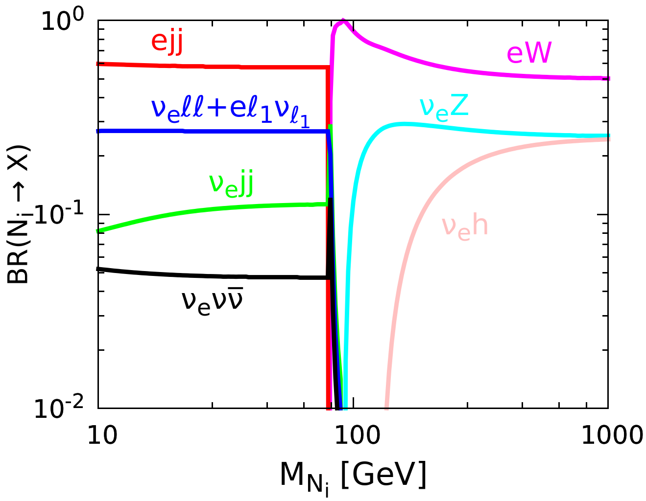
Figure 1: Branching ratios of $N_{i}$ to different final states under the assumption $V_{eN_{i}}=1,V_{\mu N_{i}}=0$ and $V_{\tau N_{i}}=0$. We show the branching ratios to three body leptonic channels $e\ell_{1}\nu_{\ell_{1}}+\nu_{e}\ell\ell$, $\nu_{e}\nu\bar{\nu}$ and semi-leptonic channels such as $ejj$ and $\nu_{e}jj$, where $\ell=e,\mu,\tau$, $\ell_{1}=\mu,\tau$. For relatively large $M_{N_{i}}$ the two body decay channels such as $eW$, $\nu_{e}Z$ and $\nu_{e}h$ dominates.

In Fig. 1, we show the branching ratios of heavy neutrinos $N_{i}$ to various final states with the assumption $V_{eN_{i}}=1,V_{\mu N_{i}}=0$ and $V_{\tau N_{i}}=0$. For mass range $M_{N_{i}}<M_{W}$, three body leptonic or semi-leptonic final states dominates, whereas for $M_{N_{i}}>M_{W}$, two body decay channels starts to dominate. Note that for large values of $M_{N}$ with $|V_{\ell N_{i}}|\neq 0$, the branching ratios can be obtained as

$$\text{BR}(N_{i}\to\ell W):\text{BR}(N_{i}\to\nu_{\ell}Z):\text{BR}(N_{i}\to\nu_{\ell}h)=2:1:1.$$

Note that for sufficiently small mixing and relatively small $M_{N_{i}}$, the heavy neutrinos are long-lived particles that can travel macroscopic distances before they decay, giving rise to displaced vertex signatures. In our study we consider mass and mixing angle to be free parameter and the mixing angle is always large enough to have prompt decay.

II.2 Triplet scalar induced tree level seesaw scenario

Here we focus on type-II seesaw scenario [105, 106, 107, 108, 109]. It introduces one heavy $SU(2)_{L}$ triplet scalar $\Delta=(\Delta^{++},\Delta^{+},\Delta^{0})^{T}$, with hypercharge $Y_{\Delta}=2$. It is convenient to describe $\Delta$ in its matrix form as

$$\Delta=\left(\begin{array}[]{cc}\Delta^{+}/\sqrt{2}&\Delta^{++}\\ \Delta^{0}&-\Delta^{+}/\sqrt{2}\end{array}\right).$$ (17)

The new triplet scalar field $\Delta$, being a triplet under $SU(2)_{L}$ interacts with the SM gauge bosons. In addition to the gauge interactions, $\Delta$ has Yukawa interaction with the SM lepton doublet. The relevant Lagrangian reads as

$${\cal L}_{{\rm type\ II}}=\left[iY_{\Delta\alpha\beta}L_{\alpha}^{T}C^{-1}\tau_{2}\Delta L_{\beta}+\text{h.c.}\right]+\left(D_{\mu}\Phi\right)^{\dagger}\left(D^{\mu}\Phi\right)+\left(D_{\mu}\Delta\right)^{\dagger}\left(D^{\mu}\Delta\right)-V(\Phi,\Delta),$$ (18)

where $Y_{\Delta}^{\alpha\beta}$ is a symmetric complex matrix, $L_{\alpha}$ are lepton doublets, $C$ is the charge conjugation operator, and $D_{\mu}$ is the covariant derivative of the related scalar field. The scalar potential $V(\Phi,\Delta)$ is given as,

$$V(\Phi,\Delta)= -m_{\Phi}^{2}\Phi^{\dagger}\Phi+\frac{\lambda}{4}(\Phi^{\dagger}\Phi)^{2}+\tilde{M}_{\Delta}^{2}{\rm Tr}\left[\Delta^{\dagger}\Delta\right]+\lambda_{2}\left[{\rm Tr}\Delta^{\dagger}\Delta\right]^{2}+\lambda_{3}{\rm Tr}\left[\Delta^{\dagger}\Delta\right]^{2}$$ (19)

$$+\left[\mu\Phi^{T}i\sigma_{2}\Delta^{\dagger}\Phi+\text{h.c.}\right]+\lambda_{1}(\Phi^{\dagger}\Phi){\rm Tr}\left[\Delta^{\dagger}\Delta\right]+\lambda_{4}\Phi^{\dagger}\Delta\Delta^{\dagger}\Phi.$$

A tiny induced VEV for the triplet characterizes the Higgs triplet UV-completion of the Weinberg operator. Minimization of the total potential $V(\Phi,\Delta)$ leads to the relations

$$\tilde{M}_{\Delta}^{2} =\displaystyle M_{\Delta}^{2}-\frac{1}{2}\left[2v_{\Delta}^{2}(\lambda_{2}+\lambda_{3})+v_{\Phi}^{2}(\lambda_{1}+\lambda_{4})\right],\,\,\text{ with }M_{\Delta}^{2}\equiv\frac{v_{\Phi}^{2}\mu}{\sqrt{2}v_{\Delta}}.$$ (20)

$$m_{\Phi}^{2} =\displaystyle\frac{1}{2}\left[\frac{v_{\Phi}^{2}\lambda}{2}+v_{\Delta}^{2}(\lambda_{1}+\lambda_{4})-2\sqrt{2}\mu v_{\Delta}\right].$$ (21)

In the limit $M_{\Delta}\gg v_{\Phi}$, which is consistent with all the existing constraints, we can solve Eq. (20) for $v_{\Delta}$. Keeping terms of $\mathcal{O}(v_{\Phi}/M_{\Delta})$ we get the small induced triplet VEV

$$v_{\Delta}\approx\frac{\mu v_{\Phi}^{2}}{\sqrt{2}\tilde{M}_{\Delta}^{2}}.$$ (22)

The light neutrino mass can be produced from the type-II scenario using the Yukawa interaction between the scalar triplet and SM lepton doublets given in Eq. 18 as

$$m_{\nu}=\sqrt{2}Y_{\Delta}v_{\Delta}=Y_{\Delta}\frac{\mu v_{\Phi}^{2}}{\tilde{M}_{\Delta}^{2}}.$$ (23)

From the observed light neutrino mass constraints, the triplet Yukawa and the triplet VEV can be written using the U_PMNS matrix depending on the neutrino oscillation data in the following way

$$Y_{\Delta}=\frac{1}{\sqrt{2}v_{\Delta}}U_{\rm{PMNS}}m_{\nu}^{\rm diag}U_{\rm{PMNS}}^{T},$$ (24)

where $m_{\nu}^{\rm diag}$ is the neutrino mass eigenvalues which further depends on the neutrino oscillation data and the normal and inverted orderings of the light neutrino masses. Eq. (22) explicitly shows that the smallness of the triplet VEV can be induced either by a small $\mu$, or by a large value for $\tilde{M}_{\Delta}$. We can write the doublet and triplet neutral fields as follows after spontaneous symmetry breaking:

$$\Delta=\frac{1}{\sqrt{2}}\begin{pmatrix}\Delta^{+}&\sqrt{2}\Delta^{++}\\ v_{\Delta}+h_{\Delta}+i\eta_{\Delta}&-~{}\Delta^{+}\end{pmatrix},~{}~{}~{}~{}~{}~{}~{}\Phi=\frac{1}{\sqrt{2}}\begin{pmatrix}\sqrt{2}{\Phi}^{+}\\ v+h_{\Phi}+i\eta_{\Phi}\end{pmatrix}.$$ (25)

Scalar sector contains 10 degrees of freedom, among which, after EW breaking, seven remain as physical fields with definite masses: $H^{\pm\pm}$, $H^{\pm}$, and the neutral Higgs bosons $h$, $H^{0}$ and $A^{0}$. The doubly-charged Higgs $H^{\pm\pm}$ is simply the $\Delta^{\pm\pm}$ present in $\Delta$. The physical masses of doubly charged Higgs bosons $H^{\pm\pm}$ can be written as:

$$m_{H^{++}}^{2}=M_{\Delta}^{2}-v_{\Delta}^{2}\lambda_{3}-\frac{\lambda_{4}}{2}v_{\Phi}^{2}.$$ (26)

The other mass eigenstates can be obtained by rotating the gauge eigenstates as shown below:

$$\left(\begin{array}[]{c}\Phi^{\pm}\\ \Delta^{\pm}\end{array}\right)=R(\beta_{\pm})\left(\begin{array}[]{c}H^{\pm}\\ G^{\pm}\end{array}\right),~{}\left(\begin{array}[]{c}h_{\Phi}\\ h_{\Delta}\end{array}\right)=R(\alpha)\left(\begin{array}[]{c}h\\ H^{0}\end{array}\right),$$

$$\left(\begin{array}[]{c}\eta_{\Phi}\\ \eta_{\Delta}\end{array}\right)=R(\beta_{0})\left(\begin{array}[]{c}A^{0}\\ G^{0}\end{array}\right),~{}R(\theta)=\left(\begin{array}[]{cc}\cos\theta&-\sin\theta\\ \sin\theta&\cos\theta\\ \end{array}\right)~{},$$

where $\beta^{\pm},\beta_{0}$ and $\alpha$ are the rotation angles with $\tan\beta^{\pm}=\frac{\sqrt{2}v_{\Delta}}{v_{\Phi}}$, $\tan\beta_{0}=\frac{2v_{\Delta}}{v_{\Phi}}$ and $\tan(2\alpha)=\frac{2B}{A-C}$ where,

$$A = \frac{\lambda}{2}{v_{\Phi}^{2}},\;\;B=v_{\Phi}(-\sqrt{2}\mu+(\lambda_{1}+\lambda_{4})v_{\Delta}),\;\;C=M_{\Delta}^{2}+2(\lambda_{2}+\lambda_{3})v_{\Delta}^{2}.$$ (29)

The two scalar fields $\Phi^{\pm}$ and $\Delta^{\pm}$ from $\Phi$ and $\Delta$ mix, giving $H^{\pm}$ and the unphysical charged Goldstone $G^{\pm}$. The physical masses of singly-charged Higgs bosons $H^{\pm}$ can be written as:

$$m_{H^{+}}^{2}=\left(M_{\Delta}^{2}-\frac{\lambda_{4}}{4}v_{\Phi}^{2}\right)\left(1+\frac{2v_{\Delta}^{2}}{v_{\Phi}^{2}}\right).$$ (30)

Similarly, $\eta_{\Delta}$ and $\eta_{\Phi}$ will mix and give rise to the CP-odd scalar $A^{0}$ and the neutral Goldstone boson $G^{0}$ which becomes the longitudinal mode of $Z$ boson. The mass of this CP-odd Higgs field $A^{0}$ has the following mass:

$$m_{A^{0}}^{2} = M_{\Delta}^{2}\left(1+\frac{4v_{\Delta}^{2}}{v_{\Phi}^{2}}\right).$$ (31)

Finally, CP-even fields $h_{\Delta}$ and $h_{\Phi}$ will mix and give rise to the SM Higgs boson $h$ and a heavy Higgs boson $H^{0}$. The masses of $h$ and $H^{0}$ have the following physical masses:

$$m_{h}^{2} = \frac{1}{2}[A+C-\sqrt{(A-C)^{2}+4B^{2}}],$$ (32)

$$m_{H^{0}}^{2} = \frac{1}{2}[A+C+\sqrt{(A-C)^{2}+4B^{2}}].$$ (33)

The triplet VEV $v_{\Delta}$ is subject to constraint coming from $\rho$ parameter. The $\rho$ parameter leads to upper bound of $\mathcal{O}(1\text{ GeV})$ on the triplet VEV $v_{\Delta}$ [1]. For $v_{\Delta}\ll v_{\Phi}$, the masses of the physical Higgs bosons can be approximated as follows:

$$m_{H^{\pm\pm}}^{2}\simeq M_{\Delta}^{2}-\frac{\lambda_{4}}{2}v_{\Phi}^{2},\,\,\,\,m_{H^{\pm}}^{2}\simeq M_{\Delta}^{2}-\frac{\lambda_{4}}{4}v_{\Phi}^{2},\,\,\,\,m_{h}^{2}\simeq 2\lambda v_{\Phi}^{2}\,\,\,\,\text{and}\,\,\,\,m_{H^{0}}^{2}\approx m_{A^{0}}^{2}\simeq M_{\Delta}^{2},$$ (34)

so their mass-squared differences are given by:

$$m_{H^{\pm}}^{2}-m_{H^{\pm\pm}}^{2}\approx m_{H^{0}/A^{0}}^{2}-m_{H^{\pm}}^{2}\approx\frac{\lambda_{4}}{4}v_{\Phi}^{2}.$$ (35)

We further define the two mass-splittings as follows:

$$\delta m_{1}=m_{H^{0}}-m_{H^{\pm}},\,\,\,\,\,\,\,\,\delta m_{2}=m_{H^{\pm}}-m_{H^{\pm\pm}}.$$ (36)

With the assumptions $v_{\Delta}\ll v_{\Phi}$ and $M_{\Delta}^{2}\gg|\lambda_{4}|v_{\Phi}^{2}$, the two mass-splittings $\delta m_{1,2}$ can be approximated as

$$\Delta m\equiv\delta m_{1,2}\approx\frac{\lambda_{4}}{8}\frac{v_{\Phi}^{2}}{M_{\Delta}}.$$ (37)

Hence, the masses of all the physical Higgs states can be written in terms of just two parameters: $m_{H^{\pm\pm}}$ and $\Delta m$. Note that $\lambda_{4}$ should be small as a relatively large value of this quartic coupling at the electroweak scale can become non-perturbative at high energies even below the Planck scale. Also the mass splitting $\Delta m=m_{H^{\pm}}-m_{H^{\pm\pm}}$ affects the electroweak precision data observables, such as $S,T$ and $U$ parameters. These put a tight constraints on the mass splitting $|\Delta m|\lesssim 40$ GeV [214, 215, 117, 114]. Note that, three different mass spectra are expected depending on the value (sign) of $\lambda_{4}$, as: $(1).\,\,\lambda_{4}=0:\,\,\Delta m\approx 0\,(m_{H^{\pm\pm}}\simeq m_{H^{\pm}}\simeq m_{H^{0}/A^{0}})$, $(2).\,\,\lambda_{4}<0:\,\,\Delta m<0\,(m_{H^{\pm\pm}}>m_{H^{\pm}}>m_{H^{0}/A^{0}})$ and $(3).\,\,\lambda_{4}>0:\,\,\Delta m>0\,(m_{H^{\pm\pm}}<m_{H^{\pm}}<m_{H^{0}/A^{0}})$. These will be important for our later discussions. The Higgs triplet has, of course, interaction with gauge bosons, as well as Yukawa couplings to the SM fermions. This opens up a number of possible decay modes. We write down all possible partial decay widths of the charged multiplets $H^{\pm\pm}$ and $H^{\pm}$ of the triplet scalar. The relevant partial decay widths of $H^{\pm\pm}$ in the case of degenerate scenario ($\delta m\approx 0$) are written below

$$\Gamma(H^{\pm\pm}\to l^{\pm}_{i}l^{\pm}_{j})=\frac{m_{H}^{\pm\pm}}{(1+\delta_{ij})8\pi}\left|\frac{m_{ij}^{\nu}}{v_{\Delta}}\right|^{2},\,\,m^{\nu}=Y_{\Delta}v_{\Delta}/\sqrt{2},$$ (38)

$$\Gamma(H^{\pm\pm}\to W^{\pm}W^{\pm})=\frac{g^{2}v^{2}_{\Delta}}{8\pi m_{H^{\pm\pm}}}\sqrt{1-\frac{4}{r^{2}_{W}}}\left[\left(2+(r_{W}/2-1)^{2}\right)\right],$$ (39)

where $r_{W}=\frac{m_{H^{\pm\pm}}}{M_{W}}$. Here $m^{\nu}$ denotes the neutrino mass matrix, $i,j$ are the generation indices. For the case of negative mass splitting $(\delta m<0)$, one must also consider the additional decay channel:

$$\Gamma(H^{\pm\pm}\to H^{\pm}W^{\pm*})=\frac{9g^{4}m_{H^{\pm\pm}}\cos^{2}\beta_{\pm}}{128\pi^{3}}G\left(\frac{m_{H^{\pm}}^{2}}{m_{H^{\pm\pm}}^{2}},\frac{m_{W}^{2}}{m_{H^{\pm\pm}}^{2}}\right),$$ (40)

where $\tan\beta_{\pm}=\frac{\sqrt{2}v_{\Delta}}{v_{\Phi}}$ and the functions $\lambda(x,y)$, $G(x,y)$ are given as

$$\lambda(x,y)=(1-x-y)^{2}-4xy~{},$$ (41)

$$G(x,y)=\frac{1}{12y}\Bigg{[}2\left(-1+x\right)^{3}-9\left(-1+x^{2}\right)y+6\left(-1+x\right)y^{2}-6\left(1+x-y\right)y\sqrt{-\lambda(x,y)}\Bigg{\{}\tan^{-1}\left(\frac{1-x+y}{\sqrt{-\lambda(x,y)}}\right)$$

$$+\tan^{-1}\left(\frac{1-x-y}{\sqrt{-\lambda(x,y)}}\right)\Bigg{\}}-3\left(1+\left(x-y\right)^{2}-2y\right)y\log x\Bigg{]}~{},$$ (42)

The relevant partial decay widths of $H^{\pm}$ in the case of degenerate scenario ($\delta m\approx 0$) are written below

$$\Gamma(H^{\pm}\to q\bar{q}^{\prime})=\frac{3m_{H^{\pm}}^{3}\sin^{2}\beta_{\pm}}{8\pi v_{\Phi}^{2}}\left[\left(\frac{m_{q}^{2}}{m_{H^{\pm}}^{2}}+\frac{m_{q^{\prime}}^{2}}{m_{H^{\pm}}^{2}}\right)\left(1-\frac{m_{q}^{2}}{m_{H^{\pm}}^{2}}-\frac{m_{q^{\prime}}^{2}}{m_{H^{\pm}}^{2}}\right)-4\frac{m_{q}^{2}}{m_{H^{\pm}}^{2}}\frac{m_{q^{\prime}}^{2}}{m_{H^{\pm}}^{2}}\right]\lambda^{\frac{1}{2}}\left(\frac{m_{q}^{2}}{m_{H^{\pm}}^{2}},\frac{m_{q^{\prime}}^{2}}{m_{H^{\pm}}^{2}}\right),$$ (43)

$$\Gamma(H^{\pm}\to\ell_{i}^{\pm}\nu_{j})=\frac{m_{H^{\pm}}}{8\pi v_{\Phi}^{2}}\left(\delta_{ij}m_{i}^{2}\sin^{2}\beta_{\pm}+|Y^{ij}_{\Delta}|^{2}v_{\Phi}^{2}\cos^{2}\beta_{\pm}\right)\left(1-\frac{m_{i}^{2}}{m_{H^{\pm}}^{2}}\right)^{2},$$ (44)

$$\Gamma(H^{\pm}\to W^{\pm}Z)=\frac{g^{4}v_{\Delta}^{2}\cos^{2}\beta_{\pm}}{32\pi\cos^{2}\theta_{w}m_{H^{\pm}}}\left[\lambda\left(\frac{m_{W}^{2}}{m_{H^{\pm}}^{2}},\frac{m_{Z}^{2}}{m_{H^{\pm}}^{2}}\right)\right]^{1/2}\left[2+\frac{m_{H^{\pm}}^{4}}{4m_{W}^{2}m_{Z}^{2}}\left(1-\frac{m_{W}^{2}}{m_{H^{\pm}}^{2}}-\frac{m_{Z}^{2}}{m_{H^{\pm}}^{2}}\right)^{2}\right].$$ (45)

For the case of non-zero mass splitting $|\delta m|\neq 0$, one also has the following decay channels for $H^{\pm}$:

$$\Gamma(H^{\pm}\to H^{0}/AW^{\pm*})=\frac{9g^{4}m_{H^{\pm}}}{512\pi^{3}}\xi_{H^{\pm}W^{\mp}H^{0}/A}^{2}G\left(\frac{m_{H^{0}/A}^{2}}{m_{H^{\pm}}^{2}},\frac{m_{W}^{2}}{m_{H^{\pm}}^{2}}\right);\text{ for }\delta m<0,$$ (46)

$$\Gamma(H^{\pm}\to H^{\pm\pm}W^{\mp*})=\frac{9g^{4}m_{H^{\pm}}\cos^{2}\beta_{\pm}}{128\pi^{3}}G\left(\frac{m_{H^{\pm\pm}}^{2}}{m_{H^{\pm}}^{2}},\frac{m_{W}^{2}}{m_{H^{\pm}}^{2}}\right);\text{ for }\delta m>0,$$ (47)

where $\xi_{H^{\pm}W^{\mp}\hat{\varphi}}=\cos\alpha\sin\beta_{\pm}-\sqrt{2}\sin\alpha\cos\beta_{\pm}$, $\sin\alpha\sin\beta_{\pm}+\sqrt{2}\cos\alpha\cos\beta_{\pm}$, $\sin\beta_{0}\sin\beta_{\pm}+\sqrt{2}\cos\beta_{0}\cos\beta_{\pm}$, $\text{ for }\hat{\varphi}=h^{0},~{}H^{0},~{}A$, $\tan(2\alpha)=\frac{2B}{A-C}\text{ and }\tan\beta_{0}=\frac{2v_{\Delta}}{v_{\Phi}}.$

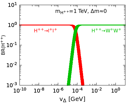
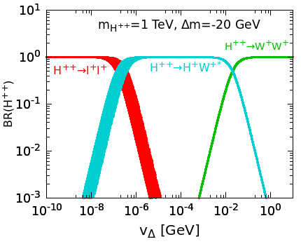
Figure 2: Branching ratios of $H^{\pm\pm}$ for mass $m_{H^{\pm\pm}}=1$ TeV with mass splitting $\Delta m\approx 0$ (left-panel) and $\Delta m=-20$ GeV (right-panel), respectively. The red, green and cyan points stand for the decay mode $H^{\pm\pm}\to\ell^{\pm}\ell^{\pm}$, $H^{\pm\pm}\to W^{\pm}W^{\pm}$ and $H^{\pm\pm}\to H^{\pm}W^{\pm*}$, respectively. Note that the decay mode $H^{\pm\pm}\to H^{\pm}W^{\pm*}$ is only open when mass-splitting is negative and further dominates in the intermediate triplet VEV region when mass-splitting is relatively large. The Dirac phase $\delta_{\text{CP}}$ is varied in the range $[-\pi:\pi]$ and other oscillation parameters are varied within their $3\sigma$ ranges whereas the lightest neutrino mass is varied in the range $10^{-4}\,\text{eV}\leq m_{\text{lightest}}<0.1\,\text{eV}$.

In Fig. 2, we display the branching ratios of $H^{\pm\pm}$ for $m_{H^{\pm\pm}}=1$ TeV with mass splitting $\Delta m\approx 0$ (left panel) and $\Delta m=-20$ GeV (right panel), respectively. For the case of small mass splitting, depending on the magnitude of the triplet VEV $v_{\Delta}$, $H^{\pm\pm}$ mainly decay to same-sign dileptons ($v_{\Delta}\leq 10^{-4}$ GeV) or gauge bosons ($v_{\Delta}>10^{-4}$ GeV). On the other hand from the right panel of Fig. 2 we see that with relatively large negative mass splitting, the cascade decay $H^{\pm\pm}\to H^{\pm}W^{\pm*}$ quickly dominate over the leptonic and diboson decay modes in the intermediate triplet VEV region.

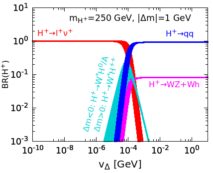
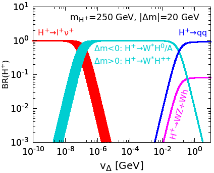
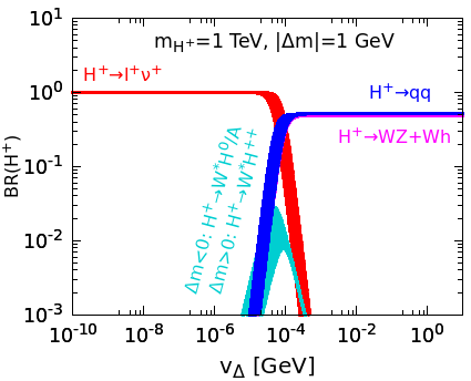
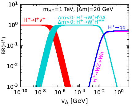
Figure 3: Branching ratios of $H^{\pm}$ for mass $m_{H^{\pm}}=250$ GeV (top-panel) and $m_{H^{\pm}}=1$ TeV (bottom-panel) with mass splitting $|\Delta m|=1\,\text{GeV}$ (left-panel) and $|\Delta m|=20$ GeV (right-panel). The singly-charged Higgs boson $H^{\pm}$ has four decay modes: (i) $\ell^{\pm}\nu$ (red), (ii) $qq$ (blue), (iii) $W^{\pm}Z+W^{\pm}h$ (magenta) and (iv) $H^{0}/AW^{*}\,(\Delta m<0)$ (cyan) or $H^{\pm\pm}W^{\mp*}\,(\Delta m>0)$ (cyan). For large mass of $H^{\pm}$, hadronic and dibosonic decay modes almost coincides. The oscillation parameters are varied again in same manner as in Fig. 2.

The branching ratio of the singly-charged Higgs $H^{\pm}$ into various channels is depicted in Figs. 3. $H^{\pm}$ has four decay modes: (i) leptonic decay, i.e. $\ell^{\pm}\nu$, (ii) hadronic decay, i.e. $q\bar{q^{\prime}}$, (iii) diboson decay, i.e. $W^{\pm}Z$, $W^{\pm}h$ and (iv) cascade decay, i.e. $H^{0}/AW^{\pm*}$ ($\delta m<0$) or $H^{\pm\pm}W^{\mp*}$ ($\delta m>0$). When comparing the left and right panels in Fig. 3, we can see that cascade decays dominate in the intermediate triplet VEV area for relatively significant mass splitting. The branching ratio pattern for singly-charged scalar decays is extremely sensitive to mass splitting and the triplet VEV, as it is for doubly-charged scalar decays. In both Figs. 2 and 3, the band for various decay modes are due to the variation of oscillation parameters. The lightest neutrino mass is varied in the range $10^{-4}\text{ eV}\leq m_{\rm lightest}\leq 0.1\text{ eV}$. The Dirac phase $\delta_{\text{CP}}$ is varied in the range $[-\pi:\pi]$ and other oscillation parameters are varied within their $3\sigma$ ranges [118, 119].

The tightest constraint on triplet scalar comes basically from doubly charged Higgs scalar searches at LHC. One clearly sees from Fig. 2 that the collider search strategy for the doubly charged Higgs boson crucially depends on the value of the triplet VEV $v_{\Delta}$ and mass splitting $\Delta m$. The direct limit on $m_{H^{\pm\pm}}$ has been derived from collider searches of multi-lepton final states assuming $\Delta m\approx 0$. Stringent constraints on $m_{H^{\pm\pm}}$ have been placed by the 13 TeV LHC searches by analysing Drell-Yan production $pp\to H^{++}H^{--}$ and subsequent decay in the $H^{\pm\pm}\to\ell^{\pm}\ell^{\pm}$ channel. In addition to this LHC has also studied the associated production of $H^{\pm\pm}H^{\mp}$ through s-channel $W^{\pm}$ exchange, followed by $H^{\pm\pm}$ decay to charged lepton pair and $H^{\pm}\to\ell^{\pm}\nu$. This combined channel of Drell-Yan production and associated production gives the constarint $m_{H^{\pm\pm}}>820$ GeV [121] at $95\%$ C.L. ATLAS searches only include the Drell-Yan production and the bound is $m_{H^{\pm\pm}}>870$ GeV at $95\%$ C.L [120]. LEP has also searched for $H^{\pm\pm}H^{\mp\mp}$ pair production through s-channel $\gamma/Z$ exchange, with subsequent decay of $H^{\pm\pm}$ into charged lepton pairs and they put constraint as $m_{H^{\pm\pm}}>97.3$ GeV [124] at $95\%$ C.L. These limits hold only for small triplet VEV, $v_{\Delta}<10^{-4}$ GeV. For large triplet VEV $v_{\Delta}>10^{-4}$ GeV, $H^{\pm\pm}$ decay dominantly to diboson mode $W^{\pm}W^{\pm}$ and hence a search via pair-production $H^{\pm\pm}H^{\mp\mp}$ , with subsequent decay into gauge boson and further to leptonic final states is required. The ATLAS collaboration has studied this channel and constrained the doubly-charged Higgs mass around 220 GeV [122]. Searches for singly-charged and neutral scalars [145, 146, 147, 148, 149, 150], on the other hand, do not apply to the type-II seesaw because the involved couplings are $v_{\Delta}^{2}$ suppressed.

II.3 Triplet fermion induced tree level seesaw scenario

Type-III seesaw is an unique possibility to describe the origin of tiny neutrino mass and flavor mixing where SM is extended by zero hypercharge SU$(2)_{\rm L}$ triplet fermion $(\Psi)$. It allows us to generate tiny but nonzero mass term form the light neutrinos through the seesaw mechanism. We write down the Lagrangian in the following way

$$\mathcal{L}=\mathcal{L}_{\text{SM}}+\text{Tr}(\overline{\Psi}i\gamma^{\mu}D_{\mu}\Psi)-\frac{1}{2}M\text{Tr}(\overline{\Psi}\Psi^{c}+\overline{\Psi^{c}}\Psi)-\sqrt{2}(\overline{\ell_{L}}Y_{D}^{\dagger}\Psi H+H^{\dagger}\overline{\Psi}Y_{D}\ell_{L}).$$ (48)

Here $D_{\mu}$ and $M$ denote the covariant derivative and Majorana mass term respectively. $\mathcal{L}_{\text{SM}}$ is the relevant part of the SM Lagrangian involved in the type-III seesaw scenario. In this analysis we consider three generations of the triplet fremion which are degenerate in mass. Hence we consider $M$ is proportional to $\bf{1}_{3\times 3}$. $Y_{D}$ is the Dirac Yukawa coupling among the triplet fermion $(\Psi)$, SM lepton doublet $(\ell_{L})$ and SM Higgs doublet $(H)$ respectively. We suppress the generation indices for simplicity. We represent the SM candidates, the triplet fermion and its charged conjugate $(\Psi^{c}=C\overline{\Psi}^{T})$ involved in the type-III seesaw mechanism as

$$\ell_{L}=\begin{pmatrix}\nu_{L}\\ e_{L}\\ \end{pmatrix},\,\,\,H=\begin{pmatrix}h^{0}\\ h^{-}\\ \end{pmatrix},\,\,\,\Psi=\begin{pmatrix}\Sigma^{0}/\sqrt{2}&\Sigma^{+}\\ \Sigma^{-}&-\Sigma^{0}/\sqrt{2}\\ \end{pmatrix}\,\,\text{and}\,\,\Psi^{c}=\begin{pmatrix}\Sigma^{0c}/\sqrt{2}&\Sigma^{-c}\\ \Sigma^{+c}&-\Sigma^{0c}/\sqrt{2}\\ \end{pmatrix}.$$ (49)

When electroweak symmetry is broken, $h^{0}$ acquires a VEV as $h^{0}=\frac{v+h}{\sqrt{2}}$ with $v=246$ GeV. To study the mixing between $\Sigma^{\pm}$ and the SM charged leptons we write the four degrees of freedom of each $\Sigma^{\pm}$ in terms of a Dirac spinor such as $\Sigma=\Sigma_{R}^{-}+\Sigma_{R}^{+c}$ where as $\Sigma^{0}$ are two component fermions with two degrees of freedom. After electroweak symmetry breaking the corresponding Lagrangian can be written as

$$-\mathcal{L}_{\text{mass}}=\begin{pmatrix}\overline{e}_{L}&\overline{\Sigma}_{L}\\ \end{pmatrix}\begin{pmatrix}m_{\ell}&Y_{D}^{\dagger}v\\ 0&M\\ \end{pmatrix}\begin{pmatrix}e_{R}\\ \Sigma_{R}\\ \end{pmatrix}+\frac{1}{2}\begin{pmatrix}\overline{\nu_{L}^{c}}&\overline{\Sigma_{R}^{0}}\\ \end{pmatrix}\begin{pmatrix}0&Y_{D}^{T}\frac{v}{\sqrt{2}}\\ Y_{D}\frac{v}{\sqrt{2}}&M\\ \end{pmatrix}\begin{pmatrix}\nu_{L}\\ \Sigma_{R}^{0c}\\ \end{pmatrix}+\text{h. c.},$$ (50)

where $m_{\ell}$ is the Dirac mass term of the SM charged lepton. The $3\times 3$ Dirac mass of the triplets can be written as

$$M_{D}=\frac{Y_{D}^{T}v}{\sqrt{2}}.$$ (51)

Diagonalizing the neutrino mass matrix in Eq. 50 we write the light neutrino mass eigenvalue in the following as

$$m_{\nu}\simeq-\frac{v^{2}}{2}Y_{D}^{T}M^{-1}Y_{D}=M_{D}M^{-1}M_{D}^{T}.$$ (52)

The mixing between the light and heavy mass eigenstates can be obtained as $\mathcal{O}(M_{D}M^{-1})$. The light neutrino flavor eigenstate can be written in terms of the light $(\nu_{m})$ and heavy $(\Sigma_{m})$ mass eigenstates as

$$\nu=\mathcal{A}\nu_{m}+V\Sigma_{m},$$ (53)

where $V=M_{D}M^{-1}$ and $\mathcal{A}=\Big{(}1-\frac{1}{2}\tilde{\epsilon}\Big{)}U_{\text{PMNS}}$ respectively with $\tilde{\epsilon}=V^{\ast}V^{T}$ and $U_{\text{PMNS}}$ is the $3\times 3$ neutrino mixing matrix which diagonalizes the light neutrino mass matrix in the following way

$$U_{\text{PMNS}}^{T}m_{\nu}U_{\text{PMNS}}=\text{diag}(m_{1},m_{2},m_{3}).$$ (54)

Due to the presence of $\tilde{\epsilon}$ the mixing matrix $(\mathcal{A})$ becomes non-unitary, $\mathcal{A}^{\dagger}\mathcal{A}\neq 1$. Replacing the neutrino flavor eigenstates with the mass eigenstates from Eq. 53 in the SM we express the charged current (CC) interactions in the following way

$$-\mathcal{L}_{\text{CC}} = \frac{g}{\sqrt{2}}\begin{pmatrix}\overline{e}&\overline{\Sigma}\\ \end{pmatrix}\gamma^{\mu}W_{\mu}^{-}P_{L}\begin{pmatrix}(1+\frac{\epsilon}{2})U_{\text{PMNS}}&-\frac{Y_{D}^{\dagger}M^{-1}v}{\sqrt{2}}\\ 0&\sqrt{2}(1-\frac{\epsilon^{\prime}}{2})\\ \end{pmatrix}\begin{pmatrix}\nu\\ \Sigma^{0}\\ \end{pmatrix}$$ (55)

$$+ \frac{g}{\sqrt{2}}\begin{pmatrix}\overline{e}&\overline{\Sigma}\\ \end{pmatrix}\gamma^{\mu}W_{\mu}^{-}P_{R}\begin{pmatrix}0&-\sqrt{2}m_{\ell}Y_{D}^{\dagger}M^{-2}v\\ -\sqrt{2}M^{-1}Y_{D}(1-\frac{\epsilon^{\ast}}{2})V_{\text{PMNS}}^{\ast}&\sqrt{2}(1-\frac{\epsilon^{\prime^{\ast}}}{2})\end{pmatrix}\begin{pmatrix}\nu\\ \Sigma^{0}\\ \end{pmatrix}.$$

Similarly using Eq. 53 in the SM neutral current (NC) interaction for the leptons we obtain the modified NC interaction as

$$-\mathcal{L}_{\text{NC}} = \frac{g}{\cos\theta_{W}}\begin{pmatrix}\overline{e}&\overline{\Sigma}\\ \end{pmatrix}\gamma^{\mu}Z_{\mu}P_{L}\begin{pmatrix}\frac{1}{2}-\cos^{2}\theta_{W}-\epsilon&\frac{Y_{D}^{\dagger}M^{-1}v}{2}\\ \frac{M^{-1}Y_{D}v}{2}&\epsilon^{\prime}-\cos^{2}\theta_{W}\end{pmatrix}\begin{pmatrix}e\\ \Sigma\\ \end{pmatrix}$$ (56)

$$+ \frac{g}{\cos\theta_{W}}\begin{pmatrix}\overline{e}&\overline{\Sigma}\\ \end{pmatrix}\gamma^{\mu}Z_{\mu}P_{R}\begin{pmatrix}1-\cos^{2}\theta_{W}&m_{\ell}Y_{D}^{\dagger}M^{-2}v\\ M^{-2}Y_{D}m_{\ell}v&-\cos^{2}\theta_{W}\end{pmatrix}\begin{pmatrix}e\\ \Sigma\\ \end{pmatrix}$$

$$+ \begin{pmatrix}\overline{\nu}&\overline{\Sigma^{0}}\\ \end{pmatrix}\gamma^{\mu}Z_{\mu}P_{L}\begin{pmatrix}1-U_{\text{PMNS}}^{\dagger}\epsilon U_{\text{PMNS}}&\frac{U_{\text{PMNS}}^{\dagger}Y_{D}^{\dagger}M^{-1}v}{\sqrt{2}}\\ \frac{M^{-1}Y_{D}U_{\text{PMNS}}v}{\sqrt{2}}&\epsilon^{\prime}\end{pmatrix}\begin{pmatrix}\nu\\ \Sigma^{0}\\ \end{pmatrix},$$

where $\theta_{W}$ is the weak mixing angle. Now we write down the interaction Lagrangian among the triplet fermion, SM lepton doublet and SM Higgs doublet $(H)$ in the following

$$-\mathcal{L}_{H} = \frac{g}{2M_{W}}\begin{pmatrix}\overline{e}&\overline{\Sigma}\\ \end{pmatrix}hP_{L}\begin{pmatrix}-\frac{m_{\ell}}{v}(1-3\epsilon)&m_{\ell}Y_{D}^{\dagger}M^{-1}\\ Y_{D}(1-\epsilon)+M^{-2}Y_{D}m_{\ell}^{2}&Y_{D}Y_{D}^{\dagger}M^{-1}v\end{pmatrix}\begin{pmatrix}e\\ \Sigma\\ \end{pmatrix}$$ (57)

$$+ \frac{g}{2M_{W}}\begin{pmatrix}\overline{e}&\overline{\Sigma}\\ \end{pmatrix}hP_{R}\begin{pmatrix}-\frac{m_{\ell}}{v}(1-3\epsilon^{\ast})&M^{-1}Y_{D}^{\dagger}m_{\ell}\\ (1-\epsilon^{\ast})Y_{D}^{\dagger}+m_{\ell}^{2}Y_{D}^{\dagger}M^{-2}&M^{-1}Y_{D}Y_{D}^{\dagger}v\end{pmatrix}\begin{pmatrix}e\\ \Sigma\\ \end{pmatrix}$$

$$+ \begin{pmatrix}\overline{\nu}&\overline{\Sigma^{0}}\\ \end{pmatrix}hP_{L}\begin{pmatrix}\frac{\sqrt{2}m_{\nu}}{v}&U_{\text{PMNS}}^{T}m_{\nu}Y_{D}^{\dagger}M^{-1}\\ (Y_{D}-\frac{Y_{D}\epsilon}{2}-\frac{\epsilon^{\prime T}Y_{D}}{2})U_{\text{PMNS}}&\frac{Y_{D}Y_{D}^{\dagger}M^{-1}v}{\sqrt{2}}\end{pmatrix}\begin{pmatrix}\nu\\ \Sigma^{0}\\ \end{pmatrix}$$

$$+ \begin{pmatrix}\overline{e}&\overline{\Sigma^{0}}\\ \end{pmatrix}hP_{R}\begin{pmatrix}\frac{\sqrt{2}m_{\nu}}{v}&M^{-1}Y_{D}m_{\nu}U_{\text{PMNS}}^{\ast}\\ U_{\text{PMNS}}^{\ast}(Y_{D}^{\dagger}-\frac{\epsilon^{\ast}Y_{D}^{\dagger}}{2}-\frac{Y_{D}^{\dagger}\epsilon^{\prime\ast}Y_{D}}{2})&\frac{M^{-1}Y_{D}Y_{D}^{\dagger}v}{\sqrt{2}}\end{pmatrix}\begin{pmatrix}\nu\\ \Sigma^{0}\\ \end{pmatrix}.$$

The charged multiplets of the triplet fermions also interact with photon $(A_{\mu})$. The corresponding interaction Lagrangian can be derived from Eq. 48 as

$$-\mathcal{L}_{\gamma\Sigma\Sigma} = g\sin\theta_{W}\begin{pmatrix}\overline{e}&\overline{\Sigma}\\ \end{pmatrix}\gamma^{\mu}A_{\mu}P_{L}\begin{pmatrix}1&0\\ 0&1\end{pmatrix}\begin{pmatrix}e\\ \Sigma\\ \end{pmatrix}+g\sin\theta_{W}\begin{pmatrix}\overline{e}&\overline{\Sigma}\\ \end{pmatrix}\gamma^{\mu}A_{\mu}P_{R}\begin{pmatrix}1&0\\ 0&1\end{pmatrix}\begin{pmatrix}e\\ \Sigma\\ \end{pmatrix}.$$ (58)

In the Eqs. 55-57 the parameters $\epsilon=\frac{v^{2}}{2}Y_{D}^{\dagger}M^{-2}Y_{D}$ and $\epsilon^{\prime}=\frac{v^{2}}{2}M^{-1}Y_{D}Y_{D}^{\dagger}M^{-1}$ are the small quantities according to Refs. [211, 216, 153]. We neglect the effects of the higher powers (above $1$) of $\epsilon$ and $\epsilon^{\prime}$ in the calculations. Using Eq. 55 to Eq. 57, we calculate the partial decay widths of $(\Sigma^{0})$ in the following way

$$\Gamma(\Sigma^{0}\to\ell^{+}W) = \Gamma(\Sigma^{0}\to\ell^{-}W)=\frac{g^{2}|V_{\ell\Sigma}|^{2}}{64\pi}\Big{(}\frac{M^{3}}{M_{W}^{2}}\Big{)}\Big{(}1-\frac{M_{W}^{2}}{M^{2}}\Big{)}^{2}\Big{(}1+2\frac{M_{W}^{2}}{M^{2}}\Big{)},$$

$$\Gamma(\Sigma^{0}\to\nu Z) = \Gamma(\Sigma^{0}\to\overline{\nu}Z)=\frac{g^{2}|V_{\ell\Sigma}|^{2}}{128\pi\cos^{2}\theta_{W}}\Big{(}\frac{M^{3}}{M_{Z}^{2}}\Big{)}\Big{(}1-\frac{M_{Z}^{2}}{M^{2}}\Big{)}^{2}\Big{(}1+2\frac{M_{Z}^{2}}{M^{2}}\Big{)},$$

$$\Gamma(\Sigma^{0}\to\nu h) = \Gamma(\Sigma^{0}\to\overline{\nu}h)=\frac{g^{2}|V_{\ell\Sigma}|^{2}}{128\pi}\Big{(}\frac{M^{3}}{M_{W}^{2}}\Big{)}\Big{(}1-\frac{M_{h}^{2}}{M^{2}}\Big{)}^{2}.$$ (59)

Similarly the partial decay widths of $(\Sigma^{\pm})$ can be calculated in terms of the mixing $(V_{\ell\Sigma})$ as

$$\Gamma(\Sigma^{\pm}\to\nu W) = \frac{g^{2}|V_{\ell\Sigma}|^{2}}{32\pi}\Big{(}\frac{M^{3}}{M_{W}^{2}}\Big{)}\Big{(}1-\frac{M_{W}^{2}}{M^{2}}\Big{)}^{2}\Big{(}1+2\frac{M_{W}^{2}}{M^{2}}\Big{)},$$

$$\Gamma(\Sigma^{\pm}\to\ell Z) = \frac{g^{2}|V_{\ell\Sigma}|^{2}}{64\pi\cos^{2}\theta_{W}}\Big{(}\frac{M^{3}}{M_{Z}^{2}}\Big{)}\Big{(}1-\frac{M_{Z}^{2}}{M^{2}}\Big{)}^{2}\Big{(}1+2\frac{M_{Z}^{2}}{M^{2}}\Big{)},$$

$$\Gamma(\Sigma^{\pm}\to\ell h) = \frac{g^{2}|V_{\ell\Sigma}|^{2}}{64\pi}\Big{(}\frac{M^{3}}{M_{W}^{2}}\Big{)}\Big{(}1-\frac{M_{h}^{2}}{M^{2}}\Big{)}^{2},$$ (60)

where $M_{W}$, $M_{Z}$ and $M_{h}$ are the SM $W$, $Z$ and Higgs boson masses respectively. The charged and neutral multiplets $\Sigma^{\pm,0}$ are degenerate in mass at the tree-level, however, radiative corrections induced by the SM gauge boson in the loop can help in lifting such degeneracy. The estimation of this mass difference $\Delta M$ can be found in [217] and that is given by

$$\Delta M=\frac{\alpha_{2}M}{4\pi}\Big{(}f\big{(}\frac{M_{W}}{M}\big{)}-\cos^{2}\theta_{W}f\big{(}\frac{M_{Z}}{M}\big{)}\Big{)},$$ (61)

where the function $f$ and $A$ are defined as $f(r)=\frac{r}{2}\big{(}2r^{3}\text{ln}\,r-2r+\sqrt{r^{2}-4}(r^{2}+2)\text{ln}\,A\big{)}$ and $A=\big{(}r^{2}-2-r\sqrt{r^{2}-4}\big{)}/2$ respectively. This mass splitting saturates at $\Delta M\approx 170$ MeV for mass $M>500$ GeV. If this mass splitting $\Delta M$ is larger than pion mass, then $\Sigma^{\pm}$ will have additional decay modes according to [217] and the corresponding partial decay widths can be written as

$$\Gamma(\Sigma^{\pm}\to\Sigma^{0}\pi^{\pm}) = \frac{2G_{F}^{2}V_{ud}^{2}\Delta M^{3}f_{\pi}^{2}}{\pi}\sqrt{1-\frac{m_{\pi}^{2}}{\Delta M^{2}}},$$

$$\Gamma(\Sigma^{\pm}\to\Sigma^{0}e\nu_{e}) = \frac{2G_{F}^{2}\Delta M^{5}}{15\pi},$$

$$\Gamma(\Sigma^{\pm}\to\Sigma^{0}\mu\nu_{\mu}) = 0.12\Gamma(\Sigma^{\pm}\to\Sigma^{0}e\nu_{e}),$$ (62)

which are independent of the free parameters. The value of the Fermi constant, $G_{F}$, is $1.1663787\times 10^{-5}$ GeV^-2, the value of the CKM parameter $(V_{ud})$ is $0.97420\pm 0.00021$ and the decay constant of the $\pi$ meson, $f_{\pi}$, is $0.13$ GeV [218]. Notice that for vanishing mixing angles $V_{\ell\Sigma}$, the $\Sigma^{\pm}$ dominantly decay into $\Sigma^{0}$, hence the decay width or the decay length is determined by $\Delta M$. Hence it is a constant. On the contrary, for very large mixing angles, $\Sigma^{0}$ decay width (decay length) is very large (very small). The Branching ratios (Br) of the neutral and charged multiplets $(\Sigma^{0,\pm})$ of the SU$(2)_{L}$ triplet fermion into SM particles are shown Fig. 4 as a function of $M$ for $V_{e}=0.019$, $V_{\mu}=0$ and $V_{\tau}=0$. The same for $V_{e}=V_{\mu}=0.0001$ and $V_{\tau}=0$ are shown in Fig. 5.

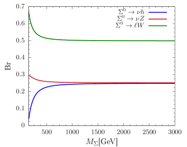
Figure 4: Branching ratio (Br) of $\Sigma^{0}$ (left) and $\Sigma^{\pm}$ (right) into the SM particles as a function of $M_{\Sigma}$ for $V_{e}=0.019$, $V_{\mu}=0$ and $V_{\tau}=0$.

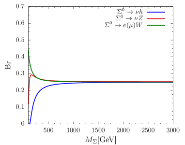
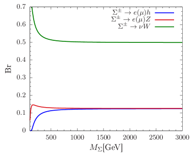
Figure 5: Branching ratio (Br) of $\Sigma^{0}$ (left) and $\Sigma^{\pm}$ (right) into the SM particles as a function of $M_{\Sigma}$ for $V_{e}=$ $V_{\mu}=0.0001$ and $V_{\tau}=0$.

Note that for large values of $M_{\Sigma}$ with $|V_{\ell}|\neq 0$, the branching ratios can be obtained as

$$\text{BR}(\Sigma^{0}\to\ell W):\text{BR}(\Sigma^{0}\to\nu_{\ell}Z):\text{BR}(\Sigma^{0}\to\nu_{\ell}h)=2:1:1,$$

$$\text{BR}(\Sigma^{\pm}\to\nu_{\ell}W^{\pm}):\text{BR}(\Sigma^{\pm}\to\ell^{\pm}Z):\text{BR}(\Sigma^{\pm}\to\ell^{\pm}h)=2:1:1.$$

III Electron photon and photon photon colliders

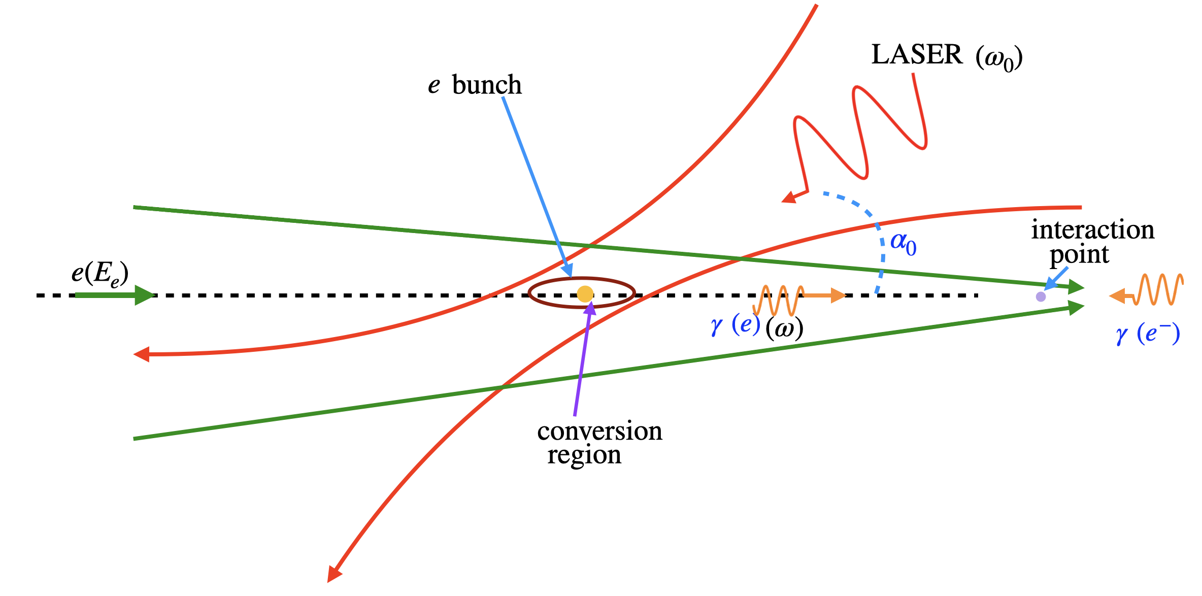
Figure 6: Schematic presentation of the proposed $e^{-}\gamma$ and $\gamma\gamma$ colliders in $e^{-}e^{+}$ collider facilities where positron can be converted into a beam of high energy photons by Compton back scattering with LASER beams. Similar procedure can be performed with electrons. In this notation $e$ represents both electron and positron. A pictorial presentation from DESY.

A linear collider with colliding electrons and positrons can be transformed into electron photon collider where positron can be replaced by a backward Compton scattered photon which comes from the collision between LASER beam with energy $\omega_{0}$ focused on a bunch of positron (it can be potentially electrons if selected) with energy $E_{e}$. The positrons beam focused towards the interaction point collide with the focused LASER beam at the conversion region and the scattered high energy photons with energy $\omega$ follow the direction of incident positron trajectories with a small angular spread. Hence they are also focused towards the interaction point. Thus produced photon beam from the Compton backward scattering can further collides with the oncoming electron beam or a similar photon beam giving rise to $e^{-}\gamma$ or $\gamma\gamma$ collisions [176, 175]. The distance between the conversion region and impact point could be $\mathcal{O}(\rm mm)$ and the schematic presentation of the $e^{-}\gamma$ and $\gamma\gamma$ collisions are shown in Fig. 6.

Unlike electron and positron beams, the $e^{-}\gamma$ colliding beams will not be mono-chromatic. The full cross section should be evaluated from the sub-process by convoluting with the structure function of photon which is basically the energy spectrum of the photons described by the Compton distribution as

$$\frac{1}{N_{\gamma}}\frac{dN_{\gamma}}{dy}\equiv F_{\gamma/e}(x,y)=\frac{1}{D(x)}\Big{(}\frac{1}{1-y}+1-y-\frac{4y}{x(1-y)}+\frac{4y^{2}}{x^{2}(1-y)^{2}}\Big{)},$$ (63)

with,

$$D(x) =\Big{(}1-\frac{4}{x}-\frac{8}{x^{2}}\Big{)}\text{ln}(1+x)+\frac{1}{2}+\frac{8}{x}-\frac{1}{2(1+x)^{2}},\,\,\,x=\frac{4E_{e}\omega_{0}}{m_{e}^{2}}\cos^{2}(\frac{\alpha_{0}}{2}),$$

$$y =\frac{\omega}{E_{e}}\leq y_{m}=\frac{\omega_{m}}{E_{e}}=\frac{x}{x+1}.$$ (64)

In the above $\omega_{0}$ is the energy of the incident photon which is scattered on the positron with energy $E_{e}$ at a small collision angle $\alpha_{0}$ which is shown in Fig. 6. Here $\omega_{m}$ is maximum achievable energy of the scattered photon and it can be large for large value of $x$. In Fig. 7, we show the energy spectrum of the photon for different choices of electron or positron beam energies $E_{e}=46$ GeV, 125 GeV, 250 GeV and 500 GeV. We see that photon energy may reach up to $80\%(90\%)$ of the energy of the initial electrons $E_{e}=250$ GeV (500 GeV) with LASER energy $\omega_{0}=1.17$ eV. Hence for larger $x$, the energy spectrum for the photon beam will be more mono-chromatic and will be peaked at high energy.

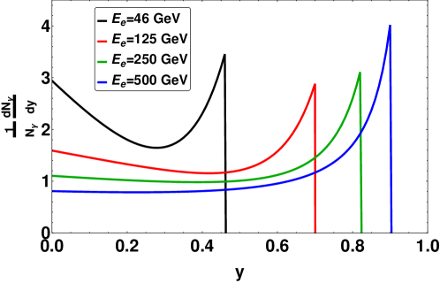
Figure 7: Energy spectrum of photons. Four lines stand for three different electron beam energies $E_{e}=46$ GeV(black), 125 GeV(red), 250 GeV(green) and 500 GeV(blue), respectively.

The total luminosity of the $e^{-}\gamma$ beam is $\mathcal{L}_{\gamma e}=\kappa\mathcal{L}_{ee}$, where $\kappa=\frac{N_{\gamma}}{N_{e}}$ is the photon conversion coefficient. This is basically the average number of high energy photons per one electron and is defined as [186]

$$\kappa=\frac{N_{\gamma}}{N_{e}}=\frac{2|\vec{v}_{e}-\vec{v}_{\gamma}|\sigma_{C}}{N_{e}}\int n_{e}n_{\gamma}dVdt$$ (65)

$\vec{v}_{e}$ and $\vec{v}_{\gamma}$ is the velocity of electrons/ positrons and incoming photons. $\sigma_{C}$ is the cross section of the Compton scattering.

III.1 Heavy Majorana neutrino production modes

The heavy neutrinos can be produced at the electron positron colliders from a variety of production modes. An interesting production of the heavy neutrinos can be considered as $e^{-}e^{+}\to N\nu$ through $t$ and $s-$channels exchanging the $W$ and $Z$ bosons, respectively. We mention these modes because of complementarity with the study of the heavy neutrino production at the electron photon collider. In electron photon colliders we can produce heavy neutrinos from $e^{-}\gamma\to NW^{-}$ involving the $t-$ channel and $s-$ channel processes. In both these case interference between these $s$ and $t-$channels take place. In both these colliders heavy neutrino production cross sections are suppressed by the square of the light-heavy mixing. For the process $e^{-}e^{+}\to N\nu$, due to the interaction with the electron we dominantly produce the first generation heavy neutrino $(N=N_{1})$, however, in the case of $Z$ mediated $s-$ channel process $e^{-}e^{+}\to N\nu$ process, second or third generation RHNs can be produced. In the following we discuss about the heavy neutrino production cross sections at the $e^{-}e^{+}$ and $e^{-}\gamma$ colliders respectively.

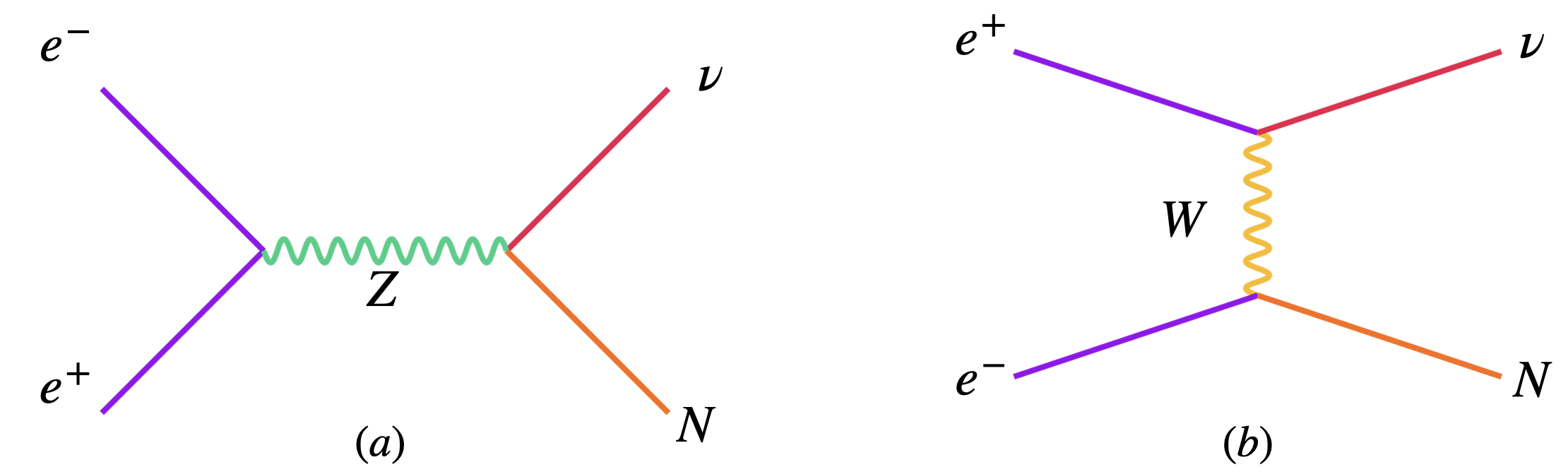
Figure 8: Heavy neutrino production processes at $e^{-}e^{+}$ colliders in association with neutrino.

Let us first consider the $e^{-}e^{+}\to\nu N_{1}$ process. Corresponding Feynman diagrams are shown in Fig. 8. We calculate the differential scattering cross section including the $s-$ channel, $t-$ channel processes and the interference term as

$$d\sigma=\frac{1}{32\pi s}\left(1-\frac{M_{N}^{2}}{s}\right)\left(|\mathcal{M}_{s}|^{2}+|\mathcal{M}_{t}|^{2}+2\text{Re}\left(\mathcal{M}_{s}^{\dagger}\mathcal{M}_{t}\right)\right),$$ (66)

The differential cross-sections are with respect to angle $\cos\theta$ in the center of mass (CM) frame. The corresponding scattering amplitude modulus squared are given below as

$$|\mathcal{M}_{s}|^{2} =\frac{g_{Z}^{4}|V_{eN_{1}}|^{2}}{16\left((s-m_{Z}^{2})^{2}+m_{Z}^{2}\Gamma_{Z}^{2}\right)}\left((1-2x_{w})^{2}(s+t)(s+t-M_{N_{1}}^{2})+4x_{w}^{2}t(t-M_{N_{1}}^{2})\right),$$ (67)

$$|\mathcal{M}_{t}|^{2} =\frac{g_{2}^{4}|V_{eN_{1}}|^{2}}{4\left((t-m_{W}^{2})^{2}+m_{W}^{2}\Gamma_{W}^{2}\right)}(s+t)(s+t-M_{N_{1}}^{2}),$$ (68)

and the interference term can be written as

$$2\text{Re}\left(\mathcal{M}_{s}^{\dagger}\mathcal{M}_{t}\right) =-\frac{g_{2}^{2}g_{Z}^{2}|V_{eN_{1}}|^{2}(1-2x_{w})}{4\left((s-m_{Z}^{2})^{2}+m_{Z}^{2}\Gamma_{Z}^{2}\right)\left((t-m_{W}^{2})^{2}+m_{W}^{2}\Gamma_{W}^{2}\right)}$$

$$(s+t)(s+t-M_{N_{1}}^{2})\left((s-m_{Z}^{2})(t-m_{W}^{2})+m_{W}m_{Z}\Gamma_{W}\Gamma_{Z}\right),$$ (69)

with $g_{Z}=\frac{e}{\sin\theta_{W}\cos\theta_{W}}$, $g_{2}=\frac{e}{\sin\theta_{W}}$, $x_{w}=\sin^{2}\theta_{W}$, $t=-\frac{1}{2}(s-M_{N}^{2})(1-\cos\theta)$ and assuming initial massless states and neglecting the light neutrino masses respectively. The total cross sections normalized by the square of the mixing for the $N_{1}\nu$ mode with respect to $M_{N_{1}}$ at different center of mass energies $(\sqrt{s})$ are shown in the left panel of Fig. 9 and those for the $N_{2}\nu$ are shown in the right panel of Fig. 9. In the second case only the $Z$ mediated $s-$ channel process participates. We find that the cross section can reach at a maximum value for $\sqrt{s}=91.2$ GeV which close to the $Z$ pole enhancing the effect of the $Z$ mediation for heavy neutrino production of any generation. The cross section decreases with the increase in $\sqrt{s}$ while going away from the $Z$ pole.

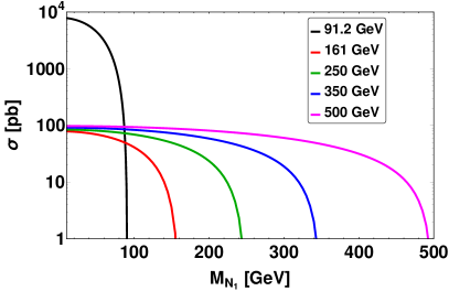
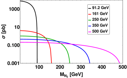
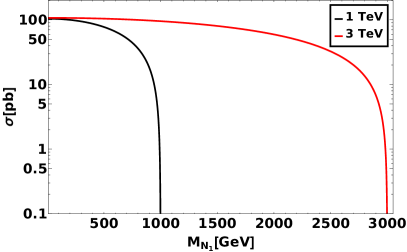
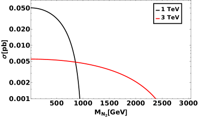
Figure 9: RHN production cross section normalized by the square of the light-heavy neutrino mixing at the linear collider considering $e^{+}e^{-}\to\nu N_{1}$ (left panel) and $e^{+}e^{-}\to\nu N_{2}$ (right panel) process at the different center of mass energies.

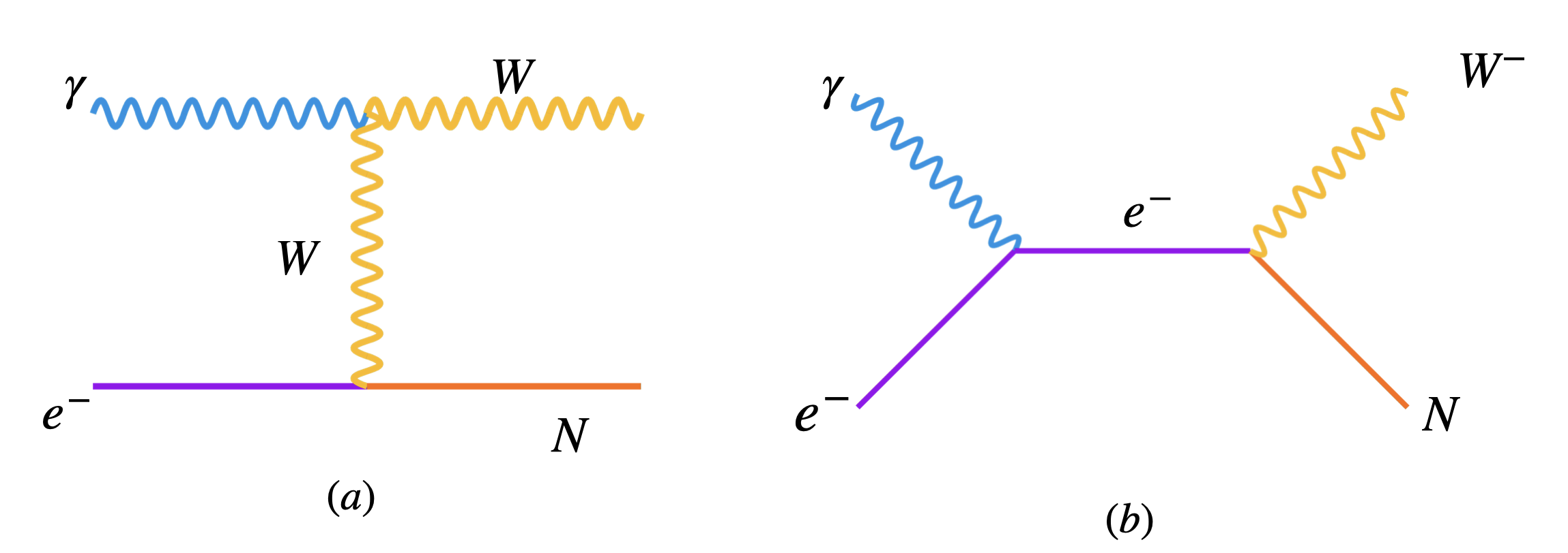
Figure 10: Heavy neutrino production processes at $e^{-}\gamma$ colliders in association with $W^{-}$.

We now calculate the $N_{1}W$ production cross section from $e^{-}\gamma$ process. Corresponding Feynman diagrams are given in Fig. 10. We estimate the differential scattering cross section of the process $\gamma e^{-}\to W^{-}N_{1}$ including the $s-$ channel and $t-$ channel processes and their interference as

$$d\sigma=\frac{1}{32\pi s}\lambda^{\frac{1}{2}}\Big{(}1,\frac{M_{N_{1}}^{2}}{s},\frac{m_{W}^{2}}{s}\Big{)}\left(|\mathcal{M}_{s}|^{2}+|\mathcal{M}_{t}|^{2}+2\text{Re}\left(\mathcal{M}_{s}^{\dagger}\mathcal{M}_{t}\right)\right),$$ (70)

and the corresponding scattering amplitude modulus squared are given below as

$$|\mathcal{M}_{s}|^{2} =\frac{g_{2}^{4}x_{w}V_{eN_{1}}^{2}}{4sm_{W}^{2}}\left(t(M_{N_{1}}^{2}-s)-m_{W}^{2}(2m_{W}^{2}+M_{N_{1}}^{2}-2(s+t))\right),$$ (71)

$$|\mathcal{M}_{t}|^{2} =\frac{g_{2}^{4}x_{w}V_{eN_{1}}^{2}}{4m_{W}^{2}\left((t-m_{W}^{2})^{2}+m_{W}^{2}\Gamma_{W}^{2}\right)}\Big{(}-m_{W}^{4}(M_{N_{1}}^{2}+5s-t)$$

$$+m_{W}^{2}(-3M_{N_{1}}^{4}-M_{N_{1}}^{2}t+5s^{2}+6st+4t^{2})$$

$$-t(-M_{N_{1}}^{4}+s^{2}+st+t^{2})\Big{)},$$ (72)

and the interference term can be written as

$$2\text{Re}\left(\mathcal{M}_{s}^{\dagger}\mathcal{M}_{t}\right) =\frac{g_{2}^{4}x_{w}V_{eN_{1}}^{2}}{4sm_{W}^{2}\left((t-m_{W}^{2})^{2}+m_{W}^{2}\Gamma_{W}^{2}\right)}(t-m_{W}^{2})\Big{(}-4m_{W}^{2}(M_{N_{1}}^{2}+s-t)+m_{W}^{2}(2M_{N_{1}}^{4}-2M_{N_{1}}^{2}(s+t)$$

$$+3s^{2})+2M_{N_{1}}^{6}-M_{N_{1}}^{4}(3s+2t)+M_{N_{1}}^{2}st+s(s^{2}+st+2t^{2})\Big{)},$$ (73)

where $t=m_{W}^{2}-\frac{s}{2}\Big{(}\sqrt{\lambda\Big{(}1,\frac{M_{N_{1}}^{2}}{s},\frac{m_{W}^{2}}{s}\Big{)}+\frac{4m_{W}^{2}}{s}}-\lambda^{\frac{1}{2}}\Big{(}1,\frac{M_{N_{1}}^{2}}{s},\frac{m_{W}^{2}}{s}\Big{)}\cos\theta\Big{)}$. The total cross section can be obtained being averaged over the photon spectrum and that can be written as

$$\braket{\sigma_{\gamma e\to N_{1}W}(\sqrt{s_{ee}})}=\int_{y_{\text{min}}}^{y_{\text{max}}}dyF_{\gamma/e}(x,y)\sigma_{\gamma e\to N_{1}W}(\sqrt{s_{e\gamma}}),$$ (74)

where $s_{ee}=4E_{e}^{2}$, $y_{\text{max}}=\frac{x}{1+x}$, $y_{\text{min}}=\frac{(M_{N_{1}}+M_{W})^{2}}{s_{ee}}$ and $s_{e\gamma}=4yE_{e}^{2}$. The analytical expression for bare process $\sigma_{\gamma e\to N_{1}W}(\sqrt{s_{e\gamma}})$ can be directly obtained from the differential scattering cross section in Eq. 70. In the right panel of Fig. 11, we show the averaged cross section along with bare cross section for two choices of heavy neutrino masses $M_{N_{1}}=100$ GeV and $M_{N_{1}}=500$ GeV respectively. The total cross sections averaged over the photon spectrum as a function of the heavy neutrino mass are shown in the right panel of Fig. 11 for different $\sqrt{s}$.

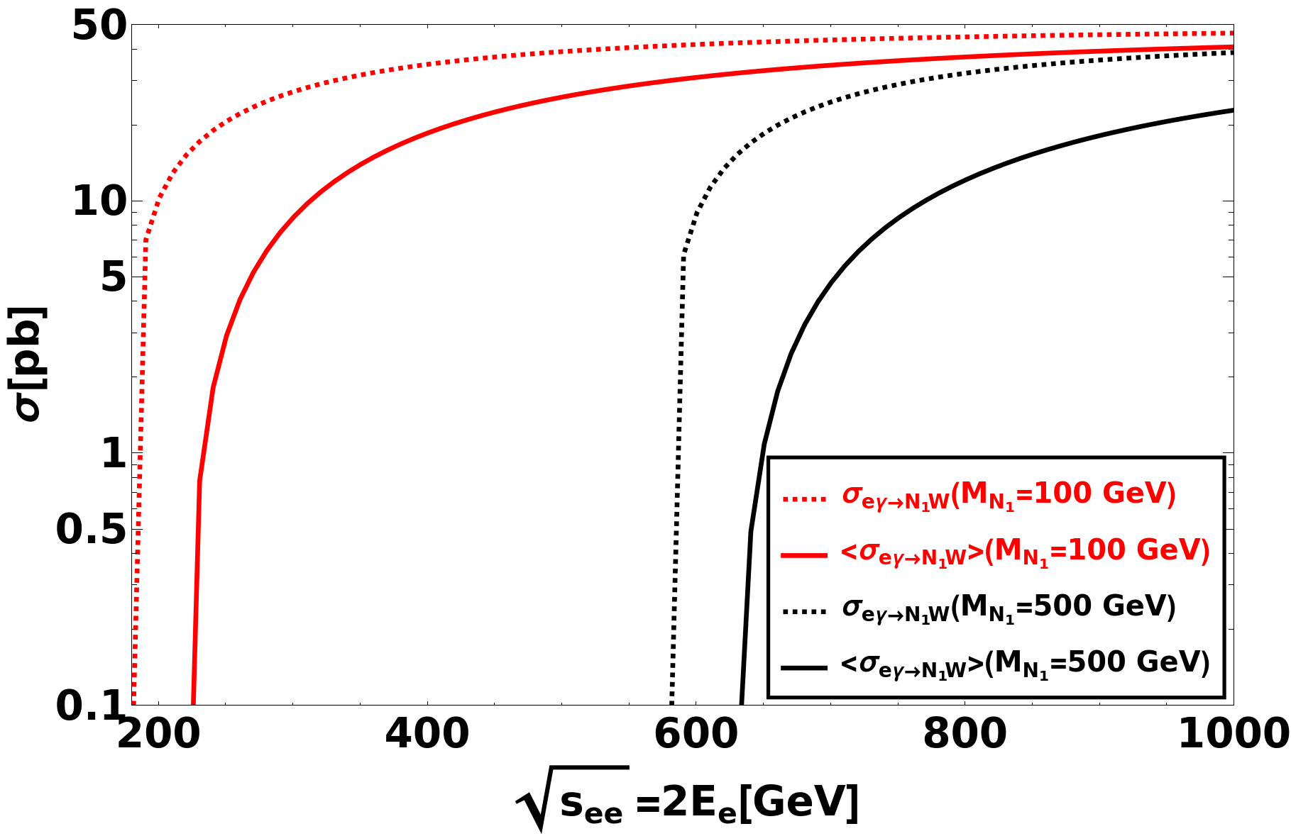
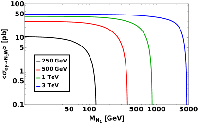
Figure 11: Left panel: Comparison of $N_{1}W$ production cross section at $e^{-}\gamma$ collider for $M_{N_{1}}=100$ GeV and $M_{N_{1}}=500$ GeV. The red and black dashed line represents the bare cross section and the red, black solid line represents the total corss section averaged over the photon spectrum normalized by the square of the mixing. Right panel: Total cross section of the $N_{1}W$ production mode at $e^{-}\gamma$ colliders for different $\sqrt{s}$ as a function of the heavy neutrino mass after averaged over photon spectrum normalized by the square of the mixing.

III.2 Triplet scalar production modes

Triplet scalar has doubly charged multiplet $(H^{\pm\pm})$ which can be tested at the $e^{-}\gamma$ colliders. The Feynman diagrams of the doubly charged scalars in association with a charged lepton ($\ell^{\pm}$) are shown in Fig. 12.

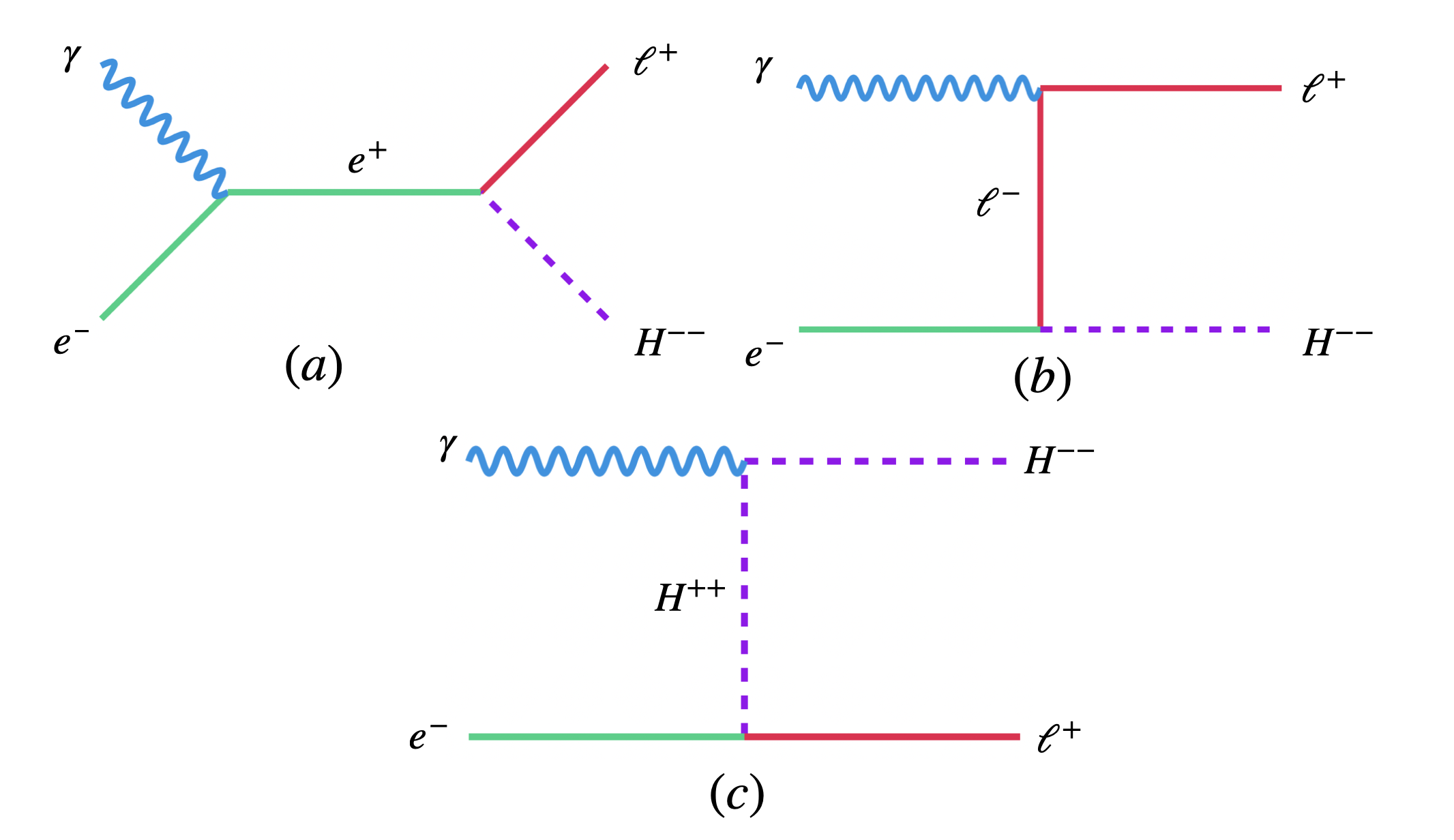
Figure 12: Feynman diagrams for the production processes $\ell^{+}H^{--}$ at the $e^{-}\gamma$ colliders where $\ell^{+}=e^{+},\mu^{+},\tau^{+}$.

In this case $\ell^{\pm}$ could be $e^{\pm}$, $\mu^{\pm}$ or $\tau^{\pm}$ which could help in testing the Lepton Flavor Violating (LFV) modes from the type-II seesaw mechanism at the $e^{-}\gamma$ coilliders. We shown the $s-$ channel and $t-$ channel processes in Fig. 12. Finally we estimate the production cross section of the $\ell^{+}H^{--}$ process and the corresponding differential scattering cross section can be written as

$$d\sigma=\frac{1}{32\pi s}\bigg{(}1-\frac{M_{H^{\pm\pm}}^{2}}{s}\bigg{)}\Big{(}|\mathcal{M}_{a}|^{2}+|\mathcal{M}_{b}|^{2}+|\mathcal{M}_{c}|^{2}+2\text{Re}\left(\mathcal{M}_{a}^{\dagger}\mathcal{M}_{b}\right)+2\text{Re}\left(\mathcal{M}_{a}^{\dagger}\mathcal{M}_{c}\right)+2\text{Re}\left(\mathcal{M}_{b}^{\dagger}\mathcal{M}_{c}\right)\Big{)},$$ (75)

where $s-$ channel and two $t-$ channel scattering amplitude modulus squared terms can be written as

$$|\mathcal{M}_{a}|^{2}=-g_{2}^{2}x_{w}|Y_{\Delta}^{e\ell}|^{2}\frac{t}{s},\,\,\,|\mathcal{M}_{b}|^{2}=-g_{2}^{2}x_{w}|Y_{\Delta}^{e\ell}|^{2}\frac{s}{t},\,\,|\mathcal{M}_{c}|^{2}=4g_{2}^{2}x_{w}|Y_{\Delta}^{e\ell}|^{2}\frac{(M_{H^{\pm\pm}}^{2}-s-t)(2M_{H^{\pm\pm}}^{2}-s-t)}{M_{H^{\pm\pm}}^{2}\Gamma_{H^{\pm\pm}}^{2}+(s+t)^{2}},$$ (76)

and the corresponding interference terms can be written as

$$2\text{Re}(\mathcal{M}_{a}^{\dagger}\mathcal{M}_{b})=2g_{2}^{2}x_{w}|Y_{\Delta}^{e\ell}|^{2}\frac{(M_{H^{\pm\pm}}^{2}-s)(M_{H^{\pm\pm}}^{2}-t)}{st},$$

$$2\text{Re}(\mathcal{M}_{a}^{\dagger}\mathcal{M}_{c})=-2g_{2}^{2}x_{w}|Y_{\Delta}^{e\ell}|^{2}\frac{(2M_{H^{\pm\pm}}^{2}-s)(s+t)(M_{H^{\pm\pm}}^{2}-s-t)}{s(M_{H^{\pm\pm}}^{2}\Gamma_{H^{\pm\pm}}^{2}+(s+t)^{2})},$$

$$2\text{Re}(\mathcal{M}_{b}^{\dagger}\mathcal{M}_{c})=-2g_{2}^{2}x_{w}|Y_{\Delta}^{e\ell}|^{2}\frac{(2M_{H^{\pm\pm}}^{2}-t)(s+t)(M_{H^{\pm\pm}}^{2}-s-t)}{t(M_{H^{\pm\pm}}^{2}\Gamma_{H^{\pm\pm}}^{2}+(s+t)^{2})}.$$ (77)

In the upper and bottom left panel of Fig. 13, we showed the averaged cross section along with bare cross section for two choices of charged Higgs mass $M_{H^{--}}=$ 300 GeV and 1000 GeV. The production

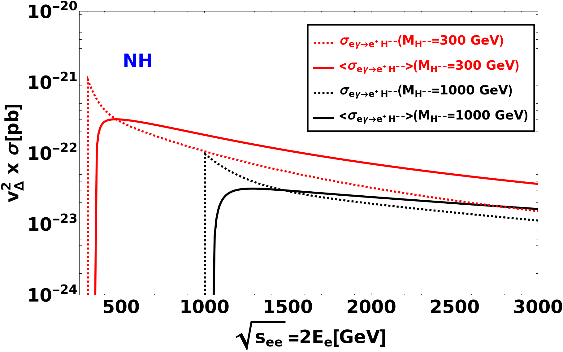
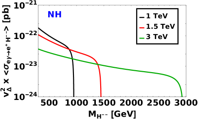
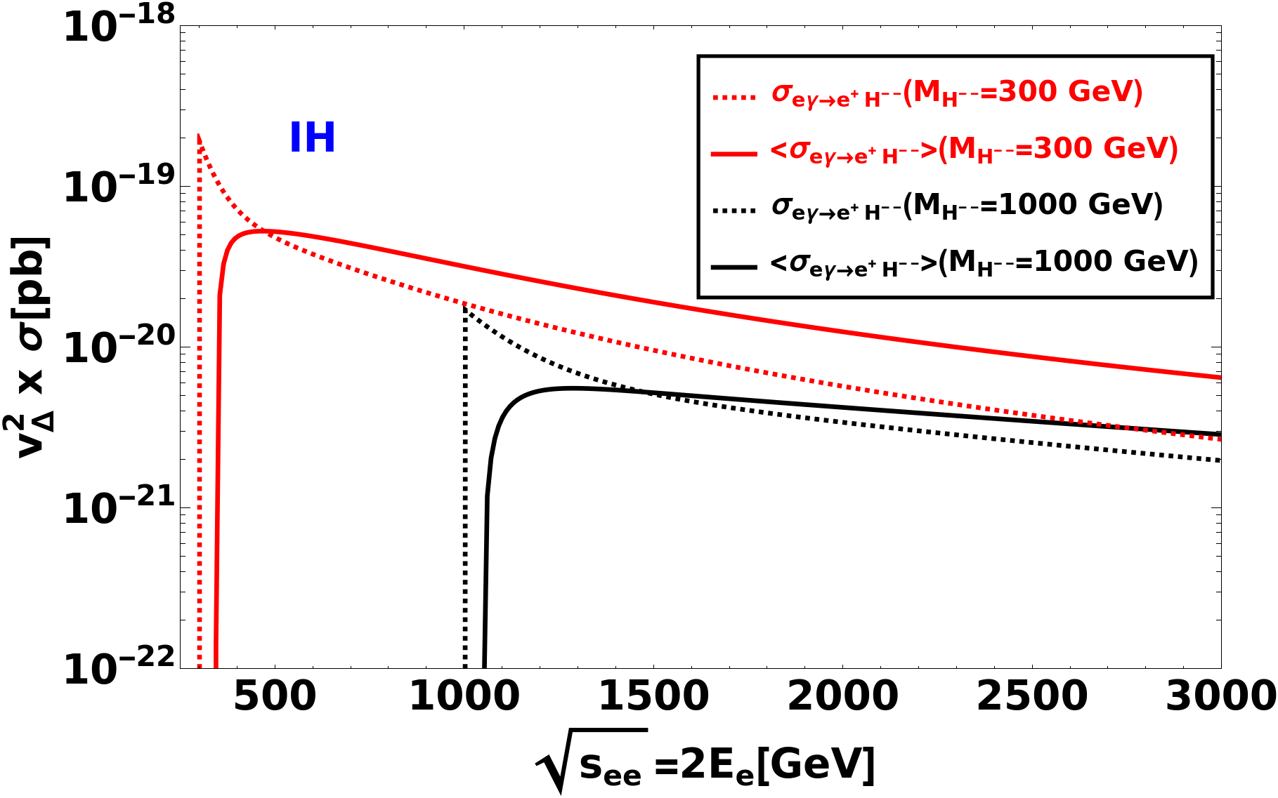
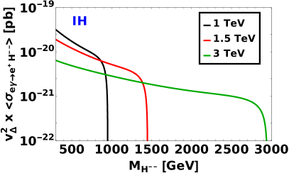
Figure 13: Production cross section of $H^{--}\ell^{+}$ process at the $e^{-}\gamma$ colliders. The upper and lower panel are for normal and inverted hierarchy. Left panel: comparison of bare and averaged cross section for charged Higgs mass $M_{H^{\pm\pm}}=300$ GeV and $M_{H^{\pm\pm}}=1000$ GeV. The red and black dashed line represents the bare cross section and the red, black solid line represents the total cross section averaged over the photon spectrum. Right panel: cross section for different $\sqrt{s}$ as a function of the charged Higgs mass after averaged over photon spectrum.

cross section of $H^{--}\ell^{+}$ as a function of $M_{H^{--}}$ for different $\sqrt{s}$ are shown in the upper right and bottom right panel. The production cross section drops with the increase in $M_{H^{--}}$ and sharply drops when $M_{H^{--}}\to\sqrt{s}$. Note that this production cross section is directly proportional to the Yukawa coupling $Y_{\Delta}$. Yukawa coupling $Y_{\Delta}$ is determined by Eq. 24 and is inversely proportional to $v_{\Delta}$. Also current measurements of neutrino oscillations parameter [119, 118] determines the pattern of Yukawa coupling $Y_{\Delta}$ and is different for normal hierarchy (NH) and inverted hierarchy (IH). This fact is clearly visible when comparing upper and bottom panel of Fig. 13. Fig. 13 is also suggests that cross section will only be sizable if one consider very small value of VEV $v_{\Delta}$. As the Yukawa coupling is inversely proportional to $v_{\Delta}$, smaller the $v_{\Delta}$, larger the Yukawa coupling. But Yukawa coupling $Y_{\Delta}$ can not be arbitrarily large as there can be potential problem with constraints coming from charged lepton flavour violating observables such as $\mu\to e\gamma$ and $\mu\to\bar{e}ee$. This actually exclude the region with $v_{\Delta}\leq 10^{-8}$ GeV [219]. With this kind of $v_{\Delta}$, the cross section will be very small and hence we decide not to discuss this production mode further.

Singly and doubly charged Higgs bosons can be produced in pair at $\gamma\gamma$ colliders. The corresponding Feynman diagrams are shown in Fig. 14.

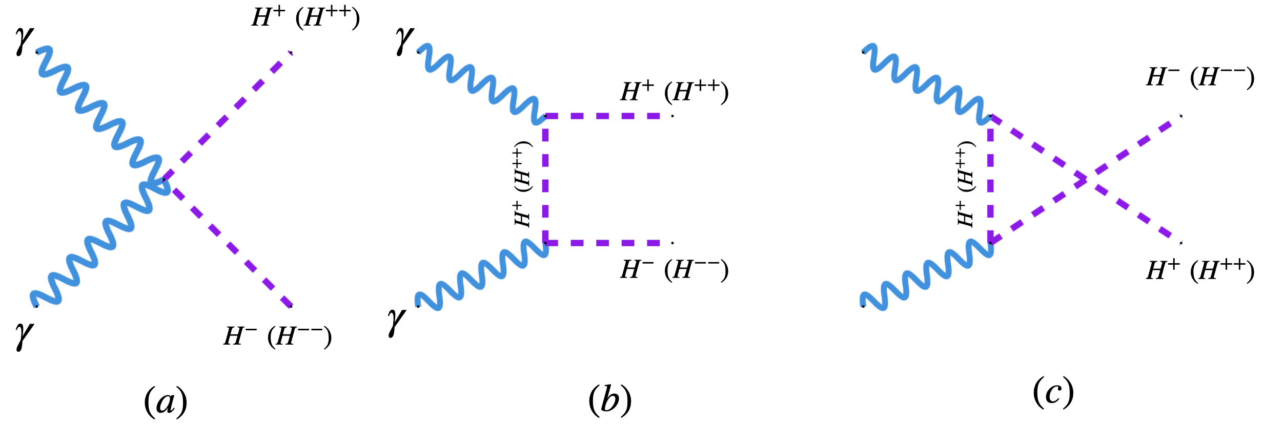
Figure 14: Production processes of the singly $(H^{\pm}H^{\mp})$ and doubly $(H^{\pm\pm}H^{\mp\mp})$ charged scalars at the $\gamma\gamma$ colliders.

The differential scattering cross section for the process $\gamma\gamma\to H^{\pm}H^{\mp}(H^{\pm\pm}H^{\mp\mp})$ is can be written as

$$d\sigma=\frac{1}{32\pi s}\sqrt{1-\frac{4M_{k}^{2}}{s}}\Big{(}|\mathcal{M}_{a}|^{2}+|\mathcal{M}_{b}|^{2}+|\mathcal{M}_{c}|^{2}+2\text{Re}\left(\mathcal{M}_{a}^{\dagger}\mathcal{M}_{b}\right)+2\text{Re}\left(\mathcal{M}_{a}^{\dagger}\mathcal{M}_{c}\right)+2\text{Re}\left(\mathcal{M}_{b}^{\dagger}\mathcal{M}_{c}\right)\Big{)}.$$ (78)

The respective terms in Eq. 78 are given below

$$|\mathcal{M}_{a}|^{2}=4Q_{k}^{4},\,\,\,\,|\mathcal{M}_{b}|^{2}=\frac{Q_{k}^{4}(M_{k}^{2}+t)^{2}}{M_{k}^{2}\Gamma_{k}^{2}+(M_{k}^{2}-t)^{2}},\,\,\,\,|\mathcal{M}_{c}|^{2}=\frac{Q_{k}^{4}(s+t-3M_{k}^{2})^{2}}{M_{k}^{2}\Gamma_{k}^{2}+(s+t-M_{k}^{2})^{2}},$$ (79)

and the interference terms can be written as

$$2\text{Re}(\mathcal{M}_{a}^{\dagger}\mathcal{M}_{b})=\frac{Q_{k}^{4}(M_{k}^{2}-t)(4M_{k}^{2}-s+4t)}{2\Big{(}M_{k}^{2}\Gamma_{k}^{2}+(M_{k}^{2}-t)^{2}\Big{)}},$$

$$2\text{Re}(\mathcal{M}_{a}^{\dagger}\mathcal{M}_{c})=\frac{Q_{k}^{4}(12M_{k}^{2}-5s-4t)(s+t-M_{k}^{2})}{2\Big{(}M_{k}^{2}\Gamma_{k}^{2}+(s+t-M_{k}^{2})^{2}\Big{)}},$$

$$2\text{Re}(\mathcal{M}_{b}^{\dagger}\mathcal{M}_{c})=\frac{Q_{k}^{4}(s-4M_{k}^{2})^{2}\Big{(}M_{k}^{2}\Gamma_{k}^{2}+(M_{k}^{2}-t)(s+t-M_{k}^{2})\Big{)}}{2\Big{(}M_{k}^{2}\Gamma_{k}^{2}+(M_{k}^{2}-t)^{2}\Big{)}\Big{(}M_{k}^{2}\Gamma_{k}^{2}+(s+t-M_{k}^{2})^{2}\Big{)}},$$ (80)

where $M_{k}=\{M_{H^{\pm}},M_{H^{\pm\pm}}\}$, $t=M_{k}^{2}+\frac{s}{2}\Big{(}\cos\theta\sqrt{1-\frac{4M_{k}^{2}}{s}}-1\Big{)}$ and $Q_{k}=e(2e)$ for $H^{\pm}(H^{\pm\pm})$. We show the $H^{\pm}$ and $H^{\pm\pm}$ pair production cross section in Fig. 15 and Fig. 16, respectively. In the left panel of Fig. 15 and 16, we showed the cross section averaged over photon spectrum along with bare cross section for two choices of charged Higgs mass $M_{H^{\pm},H^{\pm\pm}}=300$ GeV and 1000 GeV. We also show the averaged cross section as a function of charged Higgs mass $M_{H^{\pm}}$ and $M_{H^{\pm\pm}}$ for different center of mass energies in the right panel of Fig. 15 and 16. The cross section decreases with the increase in mass and falls sharply at the vicinity of $\frac{\sqrt{s}}{2}$.

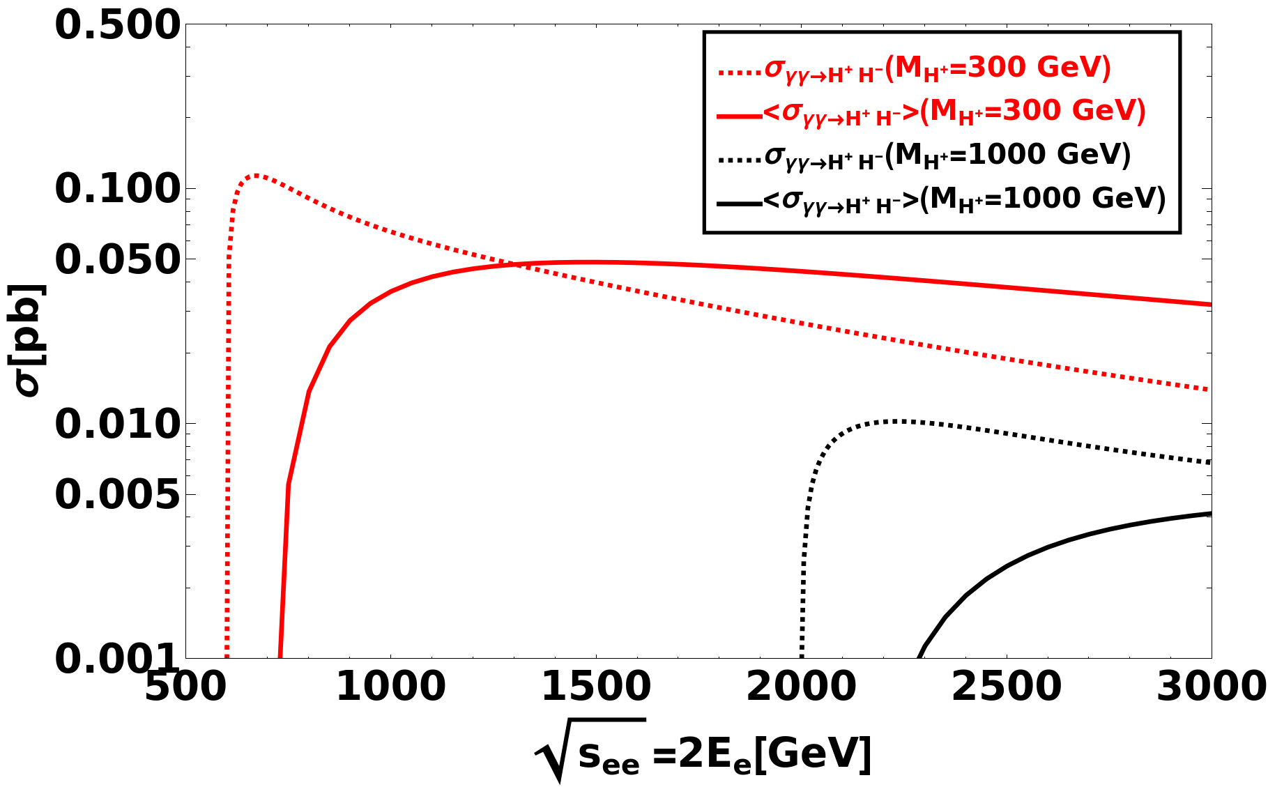
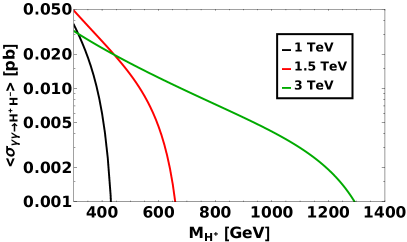
Figure 15: Production cross section of $H^{\pm}$ pair production process at the $\gamma\gamma$ colliders. Left panel: comparison of bare and averaged cross section for charged Higgs mass $M_{H^{\pm}}=300$ GeV and $M_{H^{\pm}}=1000$ GeV. The red and black dashed line represents the bare cross section and the red, black solid line represents the total corss section averaged over the photon spectrum. Right panel: cross section for different $\sqrt{s}$ as a function of the charged Higgs mass after averaging over photon spectrum.

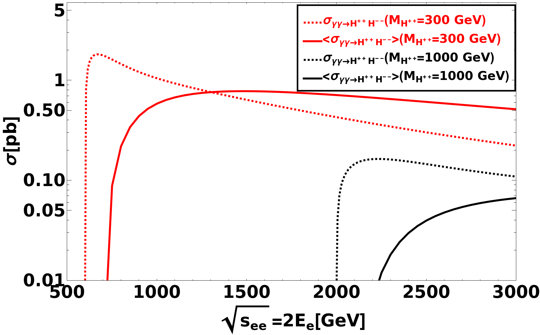
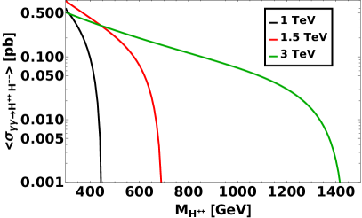
Figure 16: Same as Fig. 15 but now for process $\gamma\gamma\to H^{\pm\pm}H^{\mp\mp}$.

III.3 Triplet fermion production modes

The triplet fermions can also be tested at the $e^{-}\gamma$ collider. The triplet fermion has neutral and charged multiplets which can be produced at the $e^{-}\gamma$ colliders in association with $W^{-}$, $Z$ and $h$ bosons respectively. The Feynman diagrams of $\Sigma^{0}$ production is shown in Fig. 17.

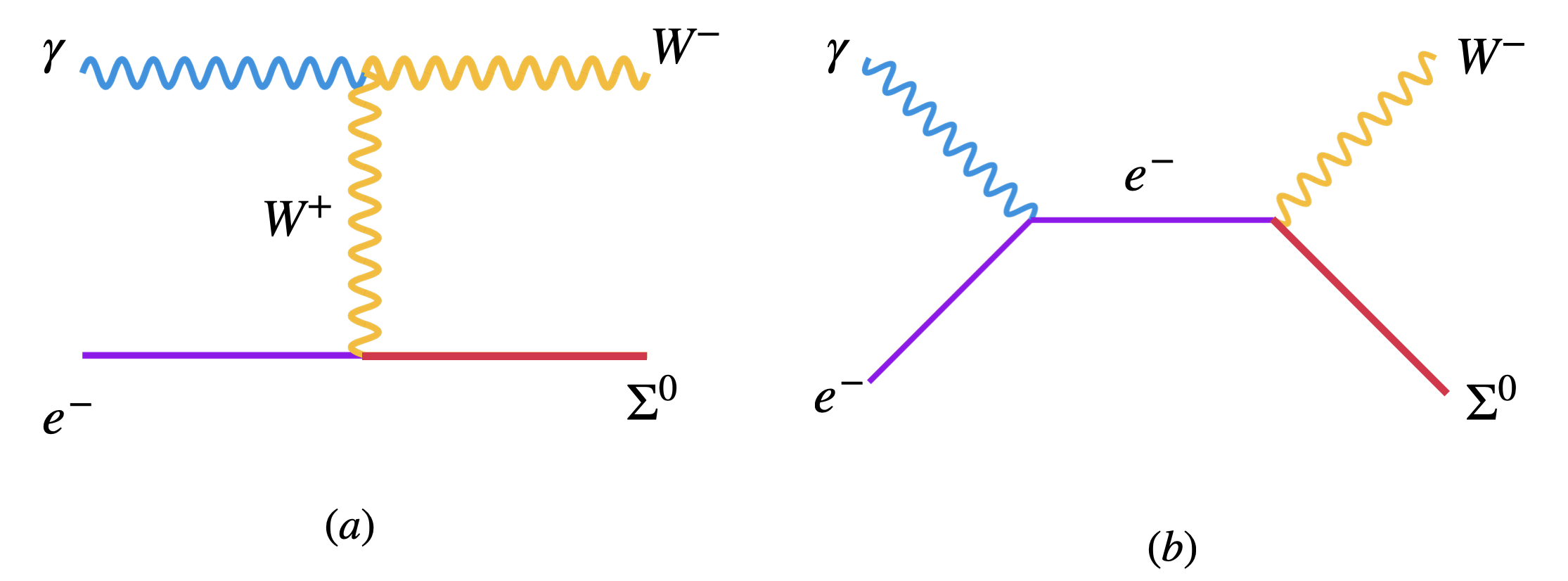
Figure 17: Neutral component of the triplet fermion production at the $e^{-}\gamma$ colliders in association with $W^{-}$.

The analytical expressions for this process is same as $e^{-}\gamma\to N_{1}W^{-}$, see Eqs. 70 and 74. We have to replace $M_{N_{1}}$ and $V_{eN_{1}}$ by $M_{\Sigma}$ and $V_{e}$, respectively. The total cross sections for different center of mass energies are shown in Fig. 18. The production cross section increases with the increase in $\sqrt{s}$. In case of type-III seesaw the triplet mass is roughly ruled out below 1 TeV from the LHC searches at 139 fb^-1 luminosity [166, 167]. Hence we consider lepton colliders with $\sqrt{s}=1.5$ TeV and 3 TeV respectively.

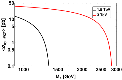
Figure 18: Total cross section of the $W\Sigma^{0}$ process in $e^{-}\gamma$ colliders as a function of $M_{\Sigma}$ for different $\sqrt{s}$ normalized by the square of the mixing.

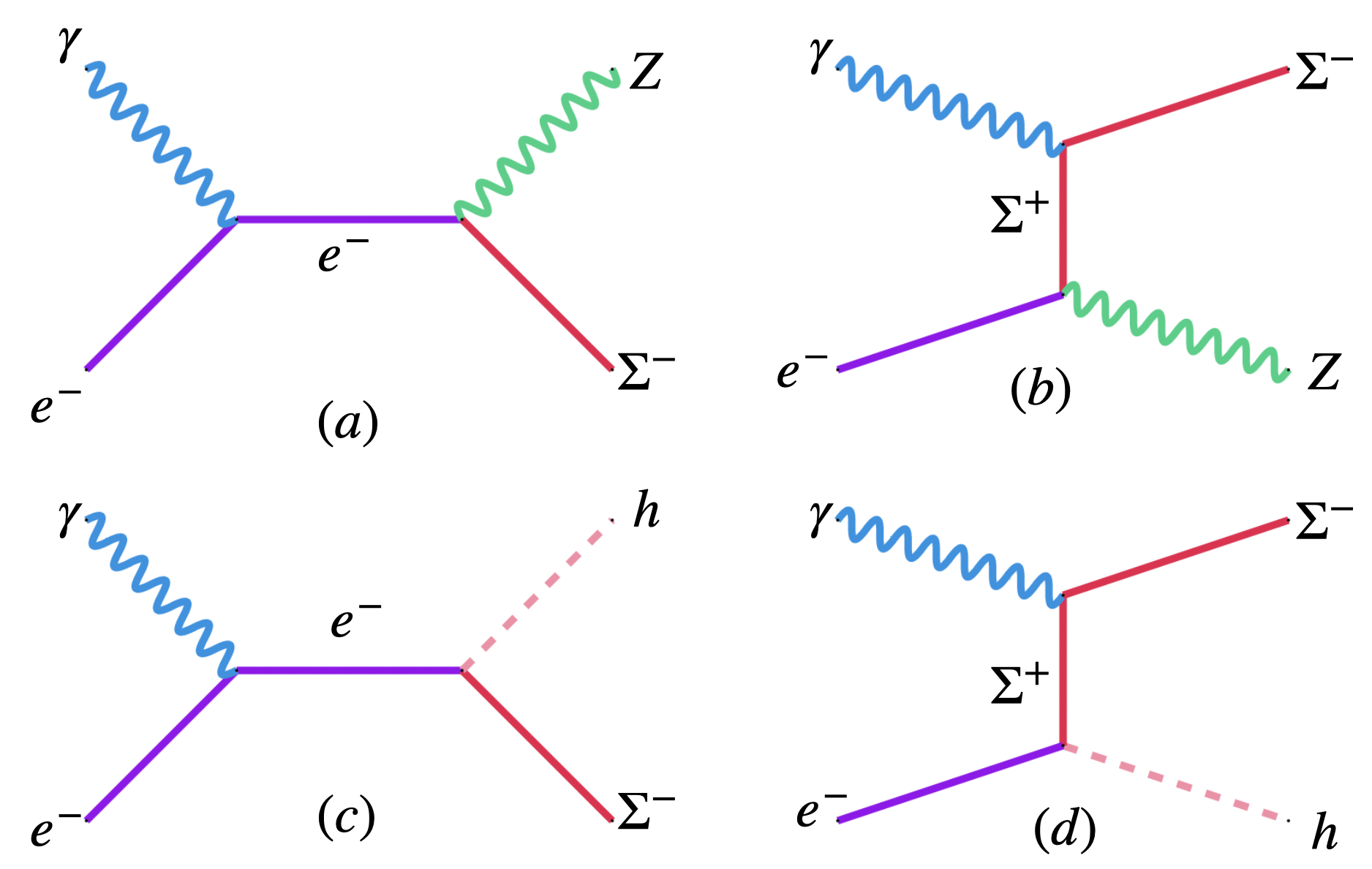
Figure 19: Charged components of the triplet fermion production at the $e^{-}\gamma$ colliders in association with $Z$ (upper panel) and $h$ (lower panel).

The charged multiplet of the triplet fermion $\Sigma^{\pm}$ can be produced in association with $Z$ and $h$ in the $e^{-}\gamma$ collider. The corresponding Feynman diagrams are shown in Fig. 19. We first describe the $e^{-}\gamma\to\Sigma^{-}Z$ process and calculate the differential scattering cross section as

$$d\sigma=\frac{1}{32\pi s}\lambda^{\frac{1}{2}}\Big{(}1,\frac{M_{\Sigma^{-}}^{2}}{s},\frac{m_{Z}^{2}}{s}\Big{)}\left(|\mathcal{M}_{s}|^{2}+|\mathcal{M}_{t}|^{2}+2\text{Re}\left(\mathcal{M}_{s}^{\dagger}\mathcal{M}_{t}\right)\right),$$ (81)

considering the $s-$ channel, $t-$ channel process and their interference. The corresponding scattering amplitude modulus squared are given below as

$$|\mathcal{M}_{s}|^{2} =\frac{V_{e}^{2}e^{4}}{4sc_{W}^{2}s_{W}^{2}m_{Z}^{2}}\Big{(}m_{Z}^{2}(2M_{\Sigma^{-}}^{2}-s-2t)+(M_{\Sigma^{-}}^{2}-s)(M_{\Sigma^{-}}^{2}-s-t)\Big{)},$$ (82)

$$|\mathcal{M}_{t}|^{2} =\frac{V_{e}^{2}e^{4}}{4c_{W}^{2}s_{W}^{2}m_{Z}^{2}\Big{(}M_{\Sigma^{-}}^{2}\Gamma_{\Sigma^{-}}^{2}+(M_{\Sigma^{-}}^{2}-t)^{2}\Big{)}}\Big{(}4M_{\Sigma^{-}}^{2}m_{Z}^{4}-m_{Z}^{2}(M_{\Sigma^{-}}^{4}-2sM_{\Sigma^{-}}^{2}+t(t+2s))$$

$$+t(M_{\Sigma^{-}}^{4}-M_{\Sigma^{-}}^{2}(s+4t)+t(s+t))\Big{)},$$ (83)

and the interference term can be written as

$$2\text{Re}\left(\mathcal{M}_{s}^{\dagger}\mathcal{M}_{t}\right) =\frac{V_{e}^{2}e^{4}}{2sc_{W}^{2}s_{W}^{2}m_{Z}^{2}\Big{(}M_{\Sigma^{-}}^{2}\Gamma_{\Sigma^{-}}^{2}+(M_{\Sigma^{-}}^{2}-t)^{2}\Big{)}}(M_{\Sigma^{-}}^{2}-t)\Big{(}-m_{Z}^{4}(M_{\Sigma^{-}}^{2}+2(s+t))$$

$$+m_{Z}^{2}(M_{\Sigma^{-}}^{2}-s)(t-M_{\Sigma^{-}}^{2})+2m_{Z}^{6}+t((M_{\Sigma^{-}}-s)^{2}+st)\Big{)},$$ (84)

where $m_{Z}$ is the $Z$ mass. Next we consider the $e^{-}\gamma\to\Sigma^{-}h$ process and calculate the differential scattering cross section as

$$d\sigma=\frac{1}{32\pi s}\lambda^{\frac{1}{2}}\Big{(}1,\frac{M_{\Sigma^{-}}^{2}}{s},\frac{m_{h}^{2}}{s}\Big{)}\left(|\mathcal{M}_{s}|^{2}+|\mathcal{M}_{t}|^{2}+2\text{Re}\left(\mathcal{M}_{s}^{\dagger}\mathcal{M}_{t}\right)\right).$$ (85)

We consider the $s-$ channel, $t-$ channel processes and their interference. The corresponding scattering amplitude modulus squared are given below as

$$|\mathcal{M}_{s}|^{2} =\frac{V_{e}^{2}(1-V_{e}^{2}-V_{\mu}^{2}-V_{\tau}^{2})^{2}e^{2}M_{\Sigma^{-}}^{2}}{sv_{H}^{2}}\Big{(}M_{\Sigma^{-}}^{2}-t\Big{)},$$ (86)

$$|\mathcal{M}_{t}|^{2} =\frac{V_{e}^{2}(1-V_{e}^{2}-V_{\mu}^{2}-V_{\tau}^{2})^{2}e^{2}M_{\Sigma^{-}}^{2}}{v_{H}^{2}\Big{(}M_{\Sigma^{-}}^{2}\Gamma_{\Sigma^{-}}^{2}+(M_{\Sigma^{-}}^{2}-t)^{2}\Big{)}}\Big{(}M_{\Sigma^{-}}^{2}(s+2m_{h}^{2})-t(s+2M_{\Sigma^{-}}^{2})\Big{)},$$ (87)

and the interference term can be written as

$$2\text{Re}\left(\mathcal{M}_{s}^{\dagger}\mathcal{M}_{t}\right) =\frac{2V_{e}^{2}(1-V_{e}^{2}-V_{\mu}^{2}-V_{\tau}^{2})^{2}e^{2}M_{\Sigma^{-}}^{2}}{sv_{H}^{2}\Big{(}M_{\Sigma^{-}}^{2}\Gamma_{\Sigma^{-}}^{2}+(M_{\Sigma^{-}}^{2}-t)^{2}\Big{)}}\Big{(}M_{\Sigma^{-}}^{2}-t\Big{)}\Big{(}m_{h}^{4}-m_{h}^{2}(M_{\Sigma^{-}}^{2}+s+t)+M_{\Sigma^{-}}^{2}(t-s)+st\Big{)},$$ (88)

where $m_{h}$ is the SM Higgs mass. The $Z\Sigma^{-}$ and $h\Sigma^{-}$ production cross section as a function of triplet mass for different center of mass energies has been shown in the left and right panel of Fig. 20.

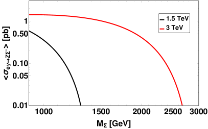
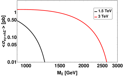
Figure 20: Total production cross section of $Z\Sigma^{-}$ and $h\Sigma^{-}$ production modes at $\gamma e$ colliders as a function of $M_{\Sigma}$ for different $\sqrt{s}$ normalized by the square of the mixing.

In the context of type-III seesaw we will consider $e^{-}\gamma\to\Sigma^{0}W^{-}$ and $Z\Sigma^{-}$ modes to probe the triplet fermions at the $e^{-}\gamma$ colliders.

IV Different signatures form the seesaw models at the colliders

In the following we consider in detail to study various final states of the singlet heavy neutrino from type-I seesaw, triplet scalar from the type-II seesaw and triplet fermion from type-III seesaw respectively. We use MadGraph [220] to generate the signal and background events and hadronize through Pythia 8 [221]. We perform the detector simulation using Delphes [222]. We used the IDEA card for $\sqrt{s}=$91.2 GeV $e^{-}e^{+}$ colldier, ILC-gen card for $\sqrt{s}=250$ GeV and ILD-card for $\sqrt{s}=500$ GeV, 1 TeV and 3 TeV $e^{-}e^{+}$, $e^{-}\gamma$ and $\gamma\gamma$ colliders respectively. To simplify the analysis, we assumed that heavy neutrinos $N_{2,3}$ are too high to acces at the considered colliders or their couplings to SM particles are zero. Further we assumed that the heavy neutrino $N_{1}$ is only coupled to electron, i.e. $V_{eN_{1}}=V_{eN}\neq 0,V_{\mu N_{1}}=V_{\tau N_{1}}=0$. Note that our analysis at $e^{-}\gamma$ and $\gamma\gamma$ collider are done assuming unpolarized electron and photon beams, which is ofcourse not true in realistic scenario as the backward Compton scattered photons are in general will be polarized. In the case of polarized beam, the signal and background behave differently for different polarization and this might weaken our obtained bound discussed below.

IV.1 Different signatures from heavy neutrinos

In our analysis we concentrate on the first generation RHN which dominantly couples with first generation of the leptons. We consider the decay mode of the heavy neutrino as $N\to eW$ followed by the hadronic decay of the $W$ boson. We study the heavy neutrino production at the $e^{-}\gamma$ colliders and we estimate the bounds on the light-heavy mixing after studying various possible signal and their SM backgrounds. We also study final states coming from heavy neutrino production at the $e^{-}e^{+}$ collider as a part of complementarity study.

IV.1.1 Heavy neutrinos at $e^{-}\gamma$ colliders

At the $e^{-}\gamma$ collider, we have considered the following set of signals after the production of the heavy neutrinos in association with $W^{-}$:

• $e^{-}\gamma\to NW^{-}\to e^{\pm}W^{\mp}W^{-}\to e^{\pm}+4j$, where $W^{\mp}$ boson coming from $N$ decays and associated $W^{-}$ boson both decays into jets. The corresponding Feynman diagram is shown in the left panel of Fig. 21. We do not show the Feynman diagram for the $s$-channel process, however, included in the analysis. Note that the final state $e^{-}+4j$ is lepton number conserving (LNC) where as $e^{+}+4j$ final state is lepton number violating (LNV). Hence one expect no SM background for $e^{+}+4j$ final state. In our analysis we combine both the LNV and LNC final state.

• $e^{-}\gamma\to NW^{-}\to e^{\pm}W^{\mp}W^{-}\to e^{-}jj\ell^{-}\nu$, where in this case associated $W^{-}$ decays leptonically. The corresponding Feynman diagram is shown in the right panel of Fig. 21. We will refer to this final state $e^{-}jj\ell^{-}\nu$ as same sign dilepton (SSDL). If $\ell^{-}=e^{-}$, we call it Same Sign Same Flavor (SSSF) scenario and if $\ell^{-}=\mu^{-}$, we call it Same Sign Different Flavor (SSDF) signal. The SSSF or SSDF signal is very interesting which may help to probe the Majorana nature of the heavy neutrino involved in this process. We study the SSDL mode combining SSSF and SSDF modes respectively.

  

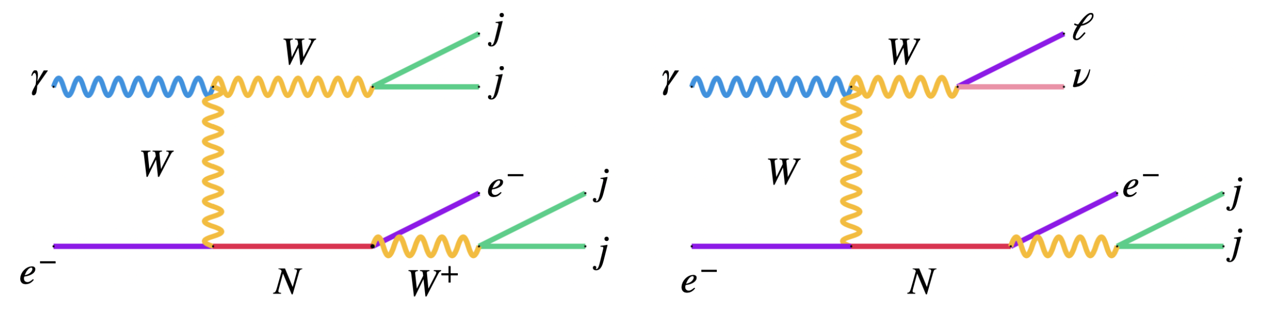
  Figure 21: $e^{\pm}+4j$ (left) and SSDL (right, $\ell^{-}=e^{-},\mu^{-}$) final states in the context of $e^{-}\gamma$ colliders. The SSDL signal is obtained combining SSSF and SSDF signals. The corresponding $s$-channel processes has been included in the analyses.

  

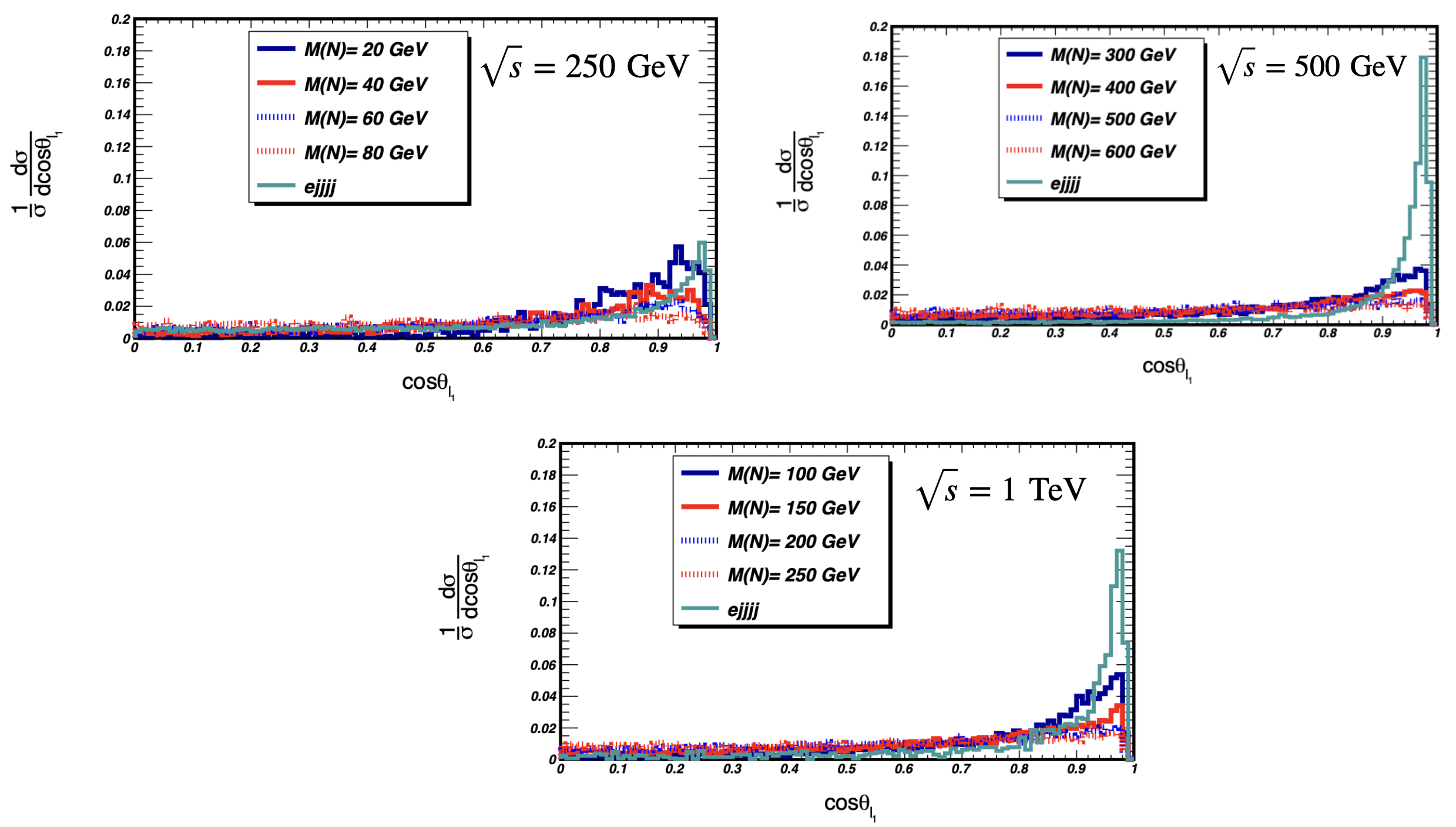
  Figure 22: The polar angle $(\cos\theta_{\ell_{1}})$ of the electron for the signal and generic background processes for $e^{-}\gamma$ collider at $\sqrt{s}=$250 GeV, 500 GeV and 1 TeV respectively for the $e^{\pm}+4j$ process. The cyan line stands for the leading SM background where as other lines stand for signal with different mass of RHN.

  In our analysis, we combine LNV and LNC channels to obtain the final states as $e^{\pm}+4j$. The LNV signal $e^{+}+4j$ is almost background free untill some $e^{+}+\text{jets}$ events appear from some radiations, however that effect will be negligible. For LNC channel $e^{-}+4j$, the leading SM backgrounds come from $e^{-}jj,e^{-}jjj$ and $e^{-}jjjj$ including initial and final state radiations. Generating the $e^{\pm}+4j$ events we show the distributions of the polar angle of the lepton, $\cos\theta_{\ell_{1}}$, of the signal and the corresponding generic background in Fig. 22 for $\sqrt{s}=250$ GeV, 500 GeV and 1 TeV respectively. The polar angle variable for the lepton $\cos\theta_{\ell}$ in Fig. 22 is defined as $\theta_{\ell}=\text{tan}^{-1}(\frac{p_{T}^{\ell}}{p_{z}^{\ell}})$, where $p_{z}^{\ell}$ is the $z$ component of the three momentum of the lepton. This is a very effective cut which reduces the SM background significantly. Note that the invariant mass cut of jets $m_{jj}$ which is coming from $W$ boson is also very effective to reduce SM background. This is because the invariant mass distribution of jets has low energy peaks which come from the hadronic activity of the low energy jets. In addition to this one can also use the invariant mass cut of the RHN. As the RHN will decay as $N\to ejj$, the invariant mass of $ejj$ will peak at $M_{ejj}\sim M_{N}$. Although we dont need to use this cut as it becomes redundant after using the lepton polar angle cut and invariant mass $m_{jj}$ cut.

  $\sqrt{s}$ (GeV)	$M_{N}$ (GeV)	Signal		Background
  		before cuts (fb)	after cuts (fb)	before cuts (fb)	after cuts (fb)
  	20	4108	63.26	102.86	4.21
  	40	3629	290.3	102.86	4.21
  250	60	2923	426.7	102.86	4.21
  	80	3460	477.8	102.86	4.21

  Table 1: Cross sections of the signal (normalized by $|V_{eN}|^{2}$) and generic background before and after cuts for $e^{-}\gamma$ collider at $\sqrt{s}=$250 GeV for the final state $e^{\pm}+4j$. We have used the following cuts: 60 GeV $<m_{jj}<$ 100 GeV, $\cos\theta_{\ell_{1}}<0.94$, $p_{T}^{j_{1,\rm leading}}>25$ GeV, $p_{T}^{j_{2,\rm trailing}}>15$ GeV, $p_{T}^{j_{3,\rm trailing}}>10$ GeV, $p_{T}^{j_{4,\rm trailing}}>7$ GeV and $p_{T}^{\ell}>12$ GeV.

  $\sqrt{s}$ (GeV)	$M_{N}$ (GeV)	Signal		Background
  		before cuts (fb)	after cuts (fb)	before cuts (fb)	after cuts (fb)
  	100	15601	3744	126.32	7.94
  	150	7279	2984	126.32	7.94
  500	200	5677	1446	126.32	1.96
  	250	3952	1288	126.32	1.96

  Table 2: Cross sections of the signal (normalized by $|V_{eN}|^{2}$) and generic background before and after cuts for $e^{-}\gamma$ collider at $\sqrt{s}=$500 GeV for the final state $e^{\pm}+4j$. We have used the following cuts: $\cos\theta_{\ell_{1}}<0.94$, 60 GeV $<m_{jj}<$ 100 GeV, $p_{T}^{j_{1,\rm leading}}>30$ GeV, $p_{T}^{j_{2,\rm trailing}}>20$ GeV, $p_{T}^{j_{3,\rm trailing}}>20$ GeV, $p_{T}^{j_{4,\rm trailing}}>10$ GeV and $p_{T}^{\ell}>10$ GeV for $M_{N_{1}}=100-150$ GeV, where as for $M_{N_{1}}>150$ GeV we used the following cuts: $\cos\theta_{\ell_{1}}<0.92$, 60 GeV $<m_{jj}<$ 100 GeV, $p_{T}^{j_{1,\rm leading}}>50$ GeV, $p_{T}^{j_{2,\rm trailing}}>40$ GeV, $p_{T}^{j_{3,\rm trailing}}>20$ GeV, $p_{T}^{j_{4,\rm trailing}}>10$ GeV and $p_{T}^{\ell}>40$ GeV.

  $\sqrt{s}$ (TeV)	$M_{N}$ (GeV)	Signal		Background
  		before cuts (fb)	after cuts (fb)	before cuts (fb)	after cuts (fb)
  	300	11161	1339	94.93	0.241
  	400	9519	1561	94.93	0.241
  1	500	7696	1301	94.93	0.082
  	600	5648	1174	94.93	0.082
  	700	3368	720.7	94.93	0.082

  Table 3: Cross sections of the signal (normalized by $|V_{eN}|^{2}$) and generic background before and after cuts for $e^{-}\gamma$ collider at $\sqrt{s}=$1 TeV for the final state $e^{\pm}+4j$. We have used the following cuts: $\cos\theta_{\ell_{1}}<0.92$, $M_{N_{1}}-40$ GeV $<m_{ejj}<M_{N_{1}}+40$, 60 GeV $<m_{jj}<$ 100 GeV, $p_{T}^{j_{1,\rm leading}}>60$ GeV, $p_{T}^{j_{2,\rm trailing}}>30$ GeV, $p_{T}^{j_{3,\rm trailing}}>20$ GeV, $p_{T}^{j_{4,\rm trailing}}>10$ GeV and $p_{T}^{\ell}>60$ GeV for $M_{N_{1}}=300-400$ GeV, whereas for $M_{N_{1}}>400$ GeV, we have used the following cuts: $\cos\theta_{\ell_{1}}<0.92$, $M_{N_{1}}-40$ GeV $<m_{ejj}<M_{N_{1}}+40$, 60 GeV $<m_{jj}<$ 100 GeV, $p_{T}^{j_{1,\rm leading}}>100$ GeV, $p_{T}^{j_{2,\rm trailing}}>50$ GeV, $p_{T}^{j_{3,\rm trailing}}>30$ GeV, $p_{T}^{j_{4,\rm trailing}}>10$ GeV and $p_{T}^{\ell}>120$ GeV.

  We study the $e^{\pm}+4j$ signal from the RHN production in a $e^{-}\gamma$ collider at the $\sqrt{s}=250$ GeV, 500 GeV and 1 TeV. The signal normalized by the square of the mixing and corresponding generic background cross sections for the $e^{\pm}+4j$ final state at $\sqrt{s}=$250 GeV, 500 GeV and 1 TeV are given in Tab. 1, 2 and 3, respectively.

  $\sqrt{s}$ (GeV)	$M_{N}$ (GeV)	Signal		Background
  		before cuts (fb)	after cuts (fb)	before cuts (fb)	after cuts (fb)
  	20	539.18	11.93	2.02	0.105
  	40	467.44	24.71	2.02	0.105
  250	60	379.17	47.05	2.02	0.105
  	80	1676.1	223.91	2.02	0.105

  Table 4: Cross sections of the signal (normalized by $|V_{eN}|^{2}$) and generic background before and after cuts for $e^{-}\gamma$ collider at $\sqrt{s}=$250 GeV for the SSDL final state. We have used the following cuts: $p_{T}^{j_{1},\rm leading}$, $p_{T}^{j_{2},\rm trailing}$ $>10$ GeV, $p_{T}^{\ell_{1},\rm leading},p_{T}^{\ell_{2},\rm trailing}>10$ GeV, 60 GeV $<m_{j_{1}j_{2}}<$ 100 GeV and $\cos\theta_{l_{1,\rm leading}}<0.9$, $\cos\theta_{l_{2,\rm trailing}}<0.92$.

  $\sqrt{s}$ (GeV)	$M_{N}$ (GeV)	Signal		Background
  		before cuts (fb)	after cuts (fb)	before cuts (fb)	after cuts (fb)
  	100	1480.1	211.82	57.64	5.31
  	150	931.49	236.61	57.64	7.42
  500	200	643.48	189.58	57.64	6.09
  	250	419.61	135.61	57.64	4.68

  Table 5: Cross sections of the signal (normalized by $|V_{eN}|^{2}$) and generic background before and after cuts for $e^{-}\gamma$ collider at $\sqrt{s}=$500 GeV for the SSDL final state. We have used the following cuts: $p_{T}^{j_{1},\rm leading}$, $p_{T}^{j_{2},\rm trailing}$ $>10$ GeV, $p_{T}^{\ell_{1},\rm leading},p_{T}^{\ell_{2},\rm trailing}>10$ GeV, 60 GeV $<m_{j_{1}j_{2}}<$ 100 GeV, $M_{N_{1}}-40$ GeV $<m_{\ell jj}<M_{N_{1}}+40$ GeV and $\cos\theta_{l_{1,\rm leading}}<0.9$, $\cos\theta_{l_{2,\rm trailing}}<0.92$.

  $\sqrt{s}$ (TeV)	$M_{N}$ (GeV)	Signal		Background
  		before cuts (fb)	after cuts (fb)	before cuts (fb)	after cuts (fb)
  	300	2596.01	123.3	128.82	1.76
  	400	2137.9	307.5	128.82	1.68
  1	500	1699.8	109.5	128.82	0.22
  	600	1236.02	190.9	128.82	0.37
  	700	733.0	139.5	128.82	0.25

  Table 6: Cross sections of the signal (normalized by $|V_{eN}|^{2}$) and generic background before and after cuts for $e^{-}\gamma$ collider at $\sqrt{s}=$1 TeV for the SSDL final state. We have used the following cuts: $p_{T}^{j_{1},\rm leading}>80$ GeV, $p_{T}^{j_{2},\rm trailing}>20$ GeV, $p_{T}^{\ell_{1},\rm leading}>120$ GeV, $p_{T}^{\ell_{2},\rm trailing}>20$ GeV, $E_{\ell_{1},\rm leading}>120$ GeV, 60 GeV $<m_{j_{1}j_{2}}<$ 100 GeV, $M_{N_{1}}-40$ GeV $<m_{\ell jj}<M_{N_{1}}+40$ GeV and $\cos\theta_{l_{1,\rm leading}}<0.92$.

  $\sqrt{s}$ (TeV)	$M_{N}$ (GeV)	Signal		Background
  		before cuts (fb)	after cuts (fb)	before cuts (fb)	after cuts (fb)
  	1000	1342.1	167.94	85.47	0.14
  3	1500	1128.67	269.75	85.47	0.13
  	2000	821.51	130.49	85.47	0.012
  	2500	325.73	77.05	85.47	0.008

  Table 7: Cross sections of the signal (normalized by $|V_{eN}|^{2}$) and generic background before and after cuts for $e^{-}\gamma$ collider at $\sqrt{s}=$3 TeV for the SSDL final state. We have used the following cuts: $p_{T}^{J}>400$ GeV, $p_{T}^{\ell_{1},\rm leading}>400$ GeV for $M_{N}=1000$ GeV, 1500 GeV and $p_{T}^{J}>800$ GeV, $p_{T}^{\ell_{1},\rm leading}>800$ GeV for $M_{N}=2000$ GeV, 2500 GeV. We have used the following additional cuts irrespective of heavy neutrino masses: 60 GeV $<m_{J}<$ 100 GeV, $M_{N_{1}}-40$ GeV $<m_{\ell J}<M_{N_{1}}+40$ GeV and $\cos\theta_{l_{1,\rm leading}}<0.92$.

  For the case of SSDL signal we again use the polar angle cut of lepton coming from RHN. We have not shown polar angle distribution as it’s behaviour almost same as in Fig. 22. In addition to this we used the leading lepton energy cut and the invariant mass of the jets $(m_{j_{1}j_{2}})$ are considered to be 60 GeV $<m_{j_{1}j_{2}}<$ 100 GeV for the $W$ boson being originated from the RHN decay. The signal normalized by the square of the mixing and corresponding generic background cross sections at $\sqrt{s}=$250 GeV, 500 GeV and 1 TeV before and after our applied cuts are given in Table. 4, 5 and 6, respectively. When necessary we also use the invariant mass of $ejj$ which peaks at RHN mass. The specific cuts we have used for each center of mass energies are mentioned in the caption of Table. 4, 5 and 6, respectively.

  We have also considered center of mass energy $\sqrt{s}=3$ TeV for the SSDL signal. As, in this case one can consider heavy RHN mass, $W$ boson from the RHN decay can be boosted so that the hadronic jets could be collimated to produce a boosted jet called fatjet ($J$). We have shown the corresponding results in Table. 7. We have used high $p_{T}$ cut for fatjet and the invariant mass cut $60\text{ GeV}\leq m_{J}\leq 100\text{ GeV}$, $M_{N_{1}}-40\text{ GeV}\leq m_{eJ}\leq M_{N_{1}}+40$ GeV.

• We study another interesting signal in the context of $e^{-}\gamma$ collider in the form of opposite sign dilepton (OSDL) final state considering $e^{-}\gamma\to NW^{-}\to e^{\pm}W^{\mp}W^{-}\to e^{-}\ell^{+}jj\nu/e^{+}\mu^{-}jj\nu$, where in this case associated $W^{-}$ decays either leptonically or hadronically. In this case we consider $\ell=e,\mu$ in the following:

  • Note that the final state $e^{+}\mu^{-}jj\nu$ is almost background free and we call it opposite sign different flavor signal. In Table. 8, we have shown the corresponding results for $\sqrt{s}=250$ GeV, 500 GeV, 1 TeV and 3 TeV, respectively. As this final state is almost background free, we have used very basic cuts such as $p_{T}^{j}>10$ GeV, $p_{T}^{\ell}>10$ GeV and $|\eta_{\ell,j}|<2.5$ to study the events.

    $\sqrt{s}$ (GeV)	$M_{N}$ (GeV)	Signal
    		before cuts (fb)	after cuts (fb)
    	20	386.6	77.33
    	40	341.6	102.5
    250	60	275.2	110.1
    	80	195.6	68.46
    	100	1481	698.3
    	150	928.5	601.4
    500	200	641.1	432.9
    	250	418.8	283.1
    	300	1161	678.4
    	400	954.1	584.1
    1000	500	756.9	471.2
    	600	547.1	339.1
    	700	322.9	190.2
    	1000	1299	879.3
    	1500	1085	804.6
    3000	2000	783.6	625.4
    	2500	309.5	262.9

    Table 8: Cross sections of the signal (normalized by $|V_{eN}|^{2}$) before and after cuts for $e^{-}\gamma$ collider at different center of mass energies for the final state $e^{+}\mu^{-}jjp_{T}^{\rm miss}$. We have used the following basic cuts: $p_{T}^{j}>10$ GeV, $p_{T}^{\ell}>10$ GeV and $|\eta_{\ell,j}|<2.5$. For $\sqrt{s}=$250 GeV, 500 GeV and 1 TeV we have demanded at least two jets, whereas for $\sqrt{s}=$3 TeV we have considered final states with one or more jets as for this one has the possibility of a fat-jet. The criteria for fat-jet are same the SSDL scenario.

  • On the other hand the final state $e^{-}\ell^{+}jj\nu$ with $\ell^{+}=e^{+},\mu^{+}$has sizable SM background from the process $e^{-}\gamma\to e^{-}W^{+}W^{-}$. In Table. 9, we show the signal and corresponding backgrounds for $\sqrt{s}=250$ GeV, 500 GeV, 1 TeV and 3 TeV, respectively. The specific cuts we have used for each center of mass energies are mentioned in the caption of Table. 9.

    $\sqrt{s}$ (GeV)	$M_{N}$ (GeV)	Signal		Background
    		before cuts (fb)	after cuts (fb)	before cuts (fb)	after cuts (fb)
    	20	866.9	83.69	2.08	0.79
    	40	752.7	121.65	2.08	0.79
    250	60	618.2	153.97	2.08	0.79
    	80	2953	670.28	2.08	0.79
    	100	2962	490.53	59.78	10.35
    	150	1860	455.06	59.78	10.35
    500	200	1287	371.46	59.78	10.35
    	250	838.75	253.79	59.78	10.35
    	300	2318	248.91	141.75	7.38
    	400	1908	361.26	141.75	7.38
    1000	500	1513	375.15	141.75	7.38
    	600	1095	240.59	141.75	2.58
    	700	644.5	151.98	141.75	2.58
    	1000	2591	91.66	120.56	0.34
    	1500	2168	242.91	120.56	0.34
    3000	2000	1572	133.91	120.56	0.017
    	2500	616.5	42.46	120.56	0.017

    Table 9: Cross sections of the signal (normalized by $|V_{eN}|^{2}$) before and after cuts for $e^{-}\gamma$ collider at different center of mass energies for the final state $e^{-}\ell^{+}jjp_{T}^{\rm miss}$. For $\sqrt{s}=$250 GeV, 500 GeV and 1 TeV we have demanded at least two jets, whereas for $\sqrt{s}=$3 TeV we have considered final states with one or more jets as for this one has the possibility of a fat-jet. The criteria for fat-jet are same the SSDL scenario. For all of considered center of mass energies we used the polar angle cuts for leptons as $|\cos\theta_{\ell_{1}}|<0.9$, $|\cos\theta_{\ell_{2}}|<0.92$ and invariant mass cut $60<m_{j_{1}j_{2}}<100$ GeV. For $\sqrt{s}=250$ GeV and 500 GeV, we have used the following basic cuts: $p_{T}^{j_{i}}>10$ GeV, $p_{T}^{\ell_{i}}>10$ GeV. For $\sqrt{s}=1000$ GeV, we used the following cuts: $p_{T}^{j_{1}}>20$ GeV, $p_{T}^{j_{2}}>10$ GeV, $p_{T}^{\ell_{1}}>90$ GeV, $p_{T}^{\ell_{2}}>20$ GeV for $M_{N}=300-500$ GeV whereas for $M_{N}>500$ GeV, we used $p_{T}^{j_{1}}>20$ GeV, $p_{T}^{j_{2}}>10$ GeV, $p_{T}^{\ell_{1}}>150$ GeV, $p_{T}^{\ell_{2}}>20$ GeV. For $\sqrt{s}=3000$ GeV, we used the following cuts: $p_{T}^{J}>180$ GeV, $p_{T}^{\ell_{1}}>450$ GeV, $p_{T}^{\ell_{2}}>30$ GeV, $60<m_{J}<100$ GeV in mass range $M_{N}=1000-1500$ GeV, where as for $M_{N}>1500$ GeV we used: $p_{T}^{J}>180$ GeV, $p_{T}^{\ell_{1}}>800$ GeV, $p_{T}^{\ell_{2}}>40$ GeV, $60<m_{J}<100$ GeV.

Using the normalized signal events from Tabs. 1-9 and the corresponding backgrounds we estimate a $2\sigma$ contour on the $M_{N_{1}}-|V_{eN}|^{2}$ plane solving the following equation

$$\sigma=\frac{\rm S\times|V_{eN}|^{2}}{\sqrt{\rm S\times|V_{eN}|^{2}+\rm B}},$$ (89)

where $S$ and $B$ stands for signal and corresponding backgrounds, respectively. We consider 5.6 ab^-1, 4 ab^-1, 8 ab^-1 and 4 ab ^-1 luminosities as benchmarks for the colliders with center of mass energies 250 GeV, 500 GeV, 1 TeV and 3 TeV respectively. The 2$\sigma$ limits are shown in Fig. 23 by the thick solid (combined $e^{\pm}+4j$ and SSDL, ‘with SSDL’) blue line. Combining the results given in Tab. 8 and 9 and applying Eq. 89 we estimate bounds on the mixing angle and it is shown by the dashed (combined $e^{\pm}+4j$ and OSDL, ‘with OSDL’) orange line.

IV.1.2 Heavy neutrinos at $e^{+}e^{-}$ colliders for complementarity

We consider $e^{+}e^{-}\to N\nu$ process followed by $N\to e^{\pm}W^{\mp}$ and hadronic decay of the $W$ boson showing $e^{\pm}+2j+p_{T}^{\rm miss}$ final state. To study this final state we consider $\sqrt{s}=91.2$ GeV, 250 GeV and 500 GeV. The distributions of the polar angle of the electron for the signal and corresponding backgrounds are same as in Fig. 22. To study this final state at $\sqrt{s}=91.2$ GeV, we consider a generic background. The signal normalized by the square of the mixing and generic background cross sections before and after cuts at $\sqrt{s}=91.2$ GeV are given in in Tab. 10. The selection cuts for the signal and generic background are mentioned in the caption of Table. 10.

$\sqrt{s}$ (GeV)	$M_{N}$ (GeV)	Signal		Background
		before cuts (fb)	after cuts (fb)	before cuts (fb)	after cuts (fb)
	20	370.21 $\times 10^{4}$	93.24$\times 10^{4}$		0.163
	40	282.10$\times 10^{4}$	105.53$\times 10^{4}$	2.52	0.163
91.2	60	156.23$\times 10^{4}$	63.16$\times 10^{4}$		0.320
	80	183.47$\times 10^{4}$	69.63$\times 10^{4}$		0.564

Table 10: Cross sections of the signal (normalized by $|V_{eN}|^{2}$) and generic background before and after cuts for $e^{-}e^{+}$ collider at $\sqrt{s}=$91.2 GeV for the final state $e^{\pm}+2j+p_{T}^{\rm miss}$. We have used the following cuts: $\cos\theta_{\ell}<0.92$, $p_{T}^{j_{1}}>15$ GeV, $p_{T}^{j_{2}}>10$ GeV, $p_{T}^{\rm miss}>15$ GeV and $p_{T}^{\ell}>10$ GeV.

To study the $e^{\pm}+2j+p_{T}^{\rm miss}$ final state at $\sqrt{s}=250$ GeV $e^{-}e^{+}$ collider, in addition to the generic background we also consider the background coming from the $ZZ$ final state where one $Z$ boson decays leptocically and the other hadronically. For relatively larger center of mass energy such as $\sqrt{s}=500$ GeV one need to also add another important background in the form of $t\overline{t}$ process. The signal normalized by the square of the mixing and generic background cross sections before and after cuts at $\sqrt{s}=250$ GeV and $\sqrt{s}=500$ GeV for $e^{\pm}+2j+p_{T}^{\rm miss}$ final state are shown in Tab. 11 and Tab. 12, respectively.

$\sqrt{s}$ (GeV)	$M_{N}$ (GeV)	Signal		Backgrounds
		before cuts (fb)	after cuts (fb)	before cuts (fb)	after cuts (fb)
	100	40510	5502	$e\nu jj:$ 4536	267
				$ZZ:$ 101	4.6
	250	38200	3097	$e\nu jj:$ 4536	99
				$ZZ:$ 101	1.3
250	150	20300	3813	$e\nu jj:$ 4536	92.4
				$ZZ:$ 101	1.3
	450	8600	2320	$e\nu jj:$ 4536	60
				$ZZ:$ 101	0.63

Table 11: Cross sections of the signal (normalized by $|V_{eN}|^{2}$) and backgrounds before and after cuts for $e^{-}e^{+}$ collider at $\sqrt{s}=$250 GeV for the final state $e^{\pm}+2j+p_{T}^{\rm miss}$. We have used the following cuts: $\cos\theta_{\ell}<0.92$, $p_{T}^{j_{1}}>30$ GeV, $p_{T}^{j_{2}}>20$ GeV, $p_{T}^{\ell}>10$ GeV and $p_{T}^{\rm miss}>20$ GeV.

$\sqrt{s}$ (GeV)	$M_{N}$ (GeV)	Signal		Backgrounds
		before cuts (fb)	after cuts (fb)	before cuts (fb)	after cuts (fb)
	100	51028	16409	$e\nu jj:$ 2251	841
				$ZZ:$ 38	1.53
				$t\overline{t}:$ 198.5	8.8
	250	24506	11023	$e\nu jj:$ 2251	392.4
				$ZZ:$ 38	0.35
				$t\overline{t}:$ 198.5	2.54
500	350	15212	6303	$e\nu jj:$ 2251	146.3
				$ZZ:$ 38	0.2
				$t\overline{t}:$ 198.5	0.6
	450	4701	2017	$e\nu jj:$ 2251	51.0
				$ZZ:$ 38	0.1
				$t\overline{t}:$ 198.5	0.06

Table 12: Cross sections of the signal (normalized by $|V_{eN}|^{2}$) and backgrounds before and after cuts for $e^{-}e^{+}$ collider at $\sqrt{s}=$500 GeV for the final state $e^{\pm}+2j+p_{T}^{\rm miss}$. We have used the following cuts: $\cos\theta_{\ell}<0.92$, $p_{T}^{j_{1}}>45$ GeV, $p_{T}^{j_{2}}>10$ GeV, $p_{T}^{\rm miss}>15$ and $p_{T}^{\ell}>50$.

Using the normalized signal events $(S)$ from Tabs. 10-12 and the corresponding backgrounds $(B)$, we estimate the significance of a $2\sigma$ contour on the $M_{N_{1}}-|V_{eN}|^{2}$ plane solving Eq. 89 with luminosities 150 ab^-1, 5.6 ab^-1 and 4 ab^-1 for $\sqrt{s}=91.2$ GeV [223], 250 GeV and 500 GeV [224, 225, 226] respectively. In this context we have scaled the previous $\sqrt{s}=$1 TeV [225] and 3 TeV [226] results using fat-jet signatures (hadronic decay of the $W$ boson) from [60] at 8 ab^-1 and 5 ab^-1 luminosities respectively. These are represented by thick, darker green dot dashed contour in Fig. 23 as ‘$e^{-}e^{+}$’. We show these bounds as a part of complementary study.

IV.1.3 Different limits on light-heavy mixing angle

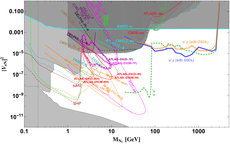
Figure 23: Limits on mixing angles of the first generation heavy neutrino compared with existing and some prospective bounds. Shaded regions are already ruled out from different searches. The closed ATLAS contours represent limits from different displaced vertex searches. The prospective limits obtained from $e^{-}\gamma$ colliders at $\sqrt{s}=250$ GeV, 500 GeV, 1 TeV and 3 TeV are shown by light blue and orange thick dashed lines. In this case ‘with SSDL’ (blue, thick solid) stands for mixings coming from combined $e^{\pm}+4j$ and SSDL modes. On the other hand ‘with OSDL’ (orange, thick dashed) stands for mixings coming from combined $e^{\pm}+4j$ and OSDL modes. The thick light green dot-dashed line represents limits for the $e^{-}e^{+}$ colliders for $\sqrt{s}=91.2$ GeV, 250 GeV, 500 GeV, 1 TeV and 3 TeV respectively as complementarity.

We compare our results with the existing bounds from a variety of experiments shown by the shaded gray region in Fig. 23. The ATLAS and CMS bounds from the SSDL signal at $\sqrt{s}=8$ TeV LHC is shown by the red dashed and dotted lines from [227, 228] respectively. The bounds from the L3 detector of LEP are shown by light green dot dashed line from [229]. The bounds from $\sqrt{s}=13$ TeV LHC using the SSDL searches from CMS [230] using cyan dot-dashed and trilepton searches from ATLAS [231] using cyan dashed and CMS [232] brown dot dashed lines respectively. The bounds obtained from the prompt (Pr) and long-lived (LL) heavy neutrinos searches from DELPHEI [233] are shown by dot dashed and dashed lines respectively. The limits from the EWPD [234, 235, 236] for the electron flavor are shown by the solid cyan line. Bounds on the mixing using long-lived particle (LLP) searches from the CMS [237] are shown by the solid magenta line for Dirac type and dot dashed purple line for Majorana types heavy neutrinos respectively. The conservative limits on the heavy neutrino mixing from the meson decay are shown by light green dashed line from [31]. The displaced vertex (DV) searches in ATLAS from the heavy neutrinos are taken from [238] where Dirac (D) and Majorana (M) types heavy neutrinos were considered for single flavor (1F) and different neutrino mass hierarchies such as normal hierarchy (NH) and inverted hierarchy (IH). The 1F case for the Dirac and Majorana types neutrinos are shown by purple and magenta dotted closed curves whereas other DV scenarios are shown by red solid (M-IH), light red dot dashed (D-IH), red dashed (D-NH) and light red dashed (M-NH) closed curves respectively. The prospective bounds obtained from the future circular collider for electron positron (FCC-ee) are shown by dashed Magenta line from [239]. The limits on the light-heavy mixing from SHiP are shown by the darker red dot dashed line from [240, 241] and those from the NA62 experiments are shown by darker red dashed line [242, 243, 244, 245]. Prospective upper limits from MATHUSLA at FCC-hh for the $W/Z$ boson decays for MATHUSLA surface version are presented by M-WZ-FCC-hh(S) and forward version M-WZ-FCC-hh(F) and the lines are shown by orange dashed and orange dotted lines respectively. The prospective limits for the heavy neutrinos produced from the $W/Z$ boson decays at the high luminosity LHC (HL LHC)are presented by M-HL-LHC-WZ and shown by solid orange line. The bounds on the heavy neutrinos obtained from the $B/D$ meson decays are represented by M-HL-LHC-BD and shown by orange dot dashed line [246]. The prospective bounds obtained from the FASER collaboration with detector radius 20 cm and 1 m are shown by the darker cyan dashed and dot dashed lines being marked as FASER20 and FASER1 respectively [247, 248]. For $M_{N_{1}}\geq 2$ GeV we find that recent bounds from LHC are stronger and rules out many existing results. Furthermore EWPD is stronger for heavier RHNs showing the gray shaded regions as ruled out parameter space. For $M_{N_{1}}\leq$ 2 GeV we find strong limits from CHARM[249, 250, 251], JNIR [252], PS191 [253], BBN [254, 255] and theoretical bounds can be obtained from the seesaw scenario [256, 257, 258] in the anti clockwise direction. We find that the prospective limits from the $e^{-}\gamma$ colliders could be compared with the bounds obtained from $e^{-}e^{+}$ colliders from $M_{N_{1}}\geq 80$ GeV.
Here we would like to mention that one can also obtain prospective bound on mixing angle $|V_{\mu N}|^{2}$ at futuristic muon collider, see Refs. [102, 103, 104] for recent studies. They found that the 3 TeV/10 TeV muon collider can probe mixing angle as $|V_{\mu N}|^{2}\sim 10^{-5}/10^{-6}$ for $M_{N}\sim\mathcal{O}(100\,\,\text{GeV})/\mathcal{O}(1\,\text{TeV})$.

IV.2 Different signatures from triplet scalars

At $\gamma\gamma$ collider, one can easily produce $H^{\pm}$ and $H^{\pm\pm}$ in pair. We found that $\gamma\gamma\to H^{+}H^{-}$ mode has nearly one order of magnitude less cross section than $\gamma\gamma\to H^{++}H^{--}$ process. Therefore we consider only the pair production of doubly charged scalar multiplet at $\gamma\gamma$ collider. As shown in Fig. 2, depending on the choices of $v_{\Delta}$ and $\Delta m$, $H^{\pm\pm}$ decays to either $\ell^{\pm}\ell^{\pm}$, $W^{\pm}W^{\pm}$ or $H^{\pm}W^{\pm*}$ with 100$\%$ branching ratio. In our analysis we will assume the mass splitting $\delta m\approx 0$ so that $H^{\pm\pm}$ either decays to $\ell^{\pm}\ell^{\pm}$ ($v_{\Delta}<10^{-4}\,\text{GeV}$) or $W^{\pm}W^{\pm}$ ($v_{\Delta}>10^{-4}\,\text{GeV}$). Hence depending on the values of $v_{\Delta}$, pair production of $H^{\pm\pm}$ can produce either four leptons $\ell_{i}^{\pm}\ell_{j}^{\pm}\ell_{k}^{\mp}\ell_{m}^{\mp}$ or $W^{\pm}W^{\pm}W^{\mp}W^{\mp}$ in the final state. The $W^{\pm}W^{\pm}W^{\mp}W^{\mp}$ mode can produce several jets in the final state following the hadronic decay of the four $W$ bosons.

Let us first discuss the leptonic mode $\gamma\gamma\to H^{\pm\pm}H^{\mp\mp}\to\ell_{i}^{\pm}\ell_{j}^{\pm}\ell_{k}^{\mp}\ell_{m}^{\mp}$ at $e^{+}e^{-}$ collider with $\sqrt{s}=3$ TeV. In this case, we assume $v_{\Delta}<10^{-4}$ GeV such that the leptonic decay from the charged Higgs $\text{BR}(H^{\pm\pm}\to\ell^{\pm}\ell^{\pm})$ can be dominant. Note that the doubly charged Higgs boson decay to leptonic final state goes as $\Gamma^{H^{\pm\pm}}_{\ell_{i}\ell_{j}}\propto|Y_{\Delta}^{ij}|^{2}$. Hence, the patterns of various leptonic channels will exactly follow the pattern of $Y_{\Delta}^{ij}$, which is determined by oscillation parameter. As a result the $\text{BR}(H^{\pm\pm}\to\ell_{i}^{\pm}\ell_{j}^{\pm})$ will also depend on the ordering of light neutrino mass. Hence, one expects that collider observables such as the cross-section $\sigma(\gamma\gamma\to H^{\pm\pm}H^{\mp\mp}\to\ell_{i}^{\pm}\ell_{j}^{\pm}\ell_{k}^{\mp}\ell_{m}^{\mp})$ may strongly correlate with neutrino mass ordering. To show that indeed this is the case, we consider three possible scenario:

• $\gamma\gamma\to H^{++}H^{--}\to\ell_{i}^{+}\ell_{j}^{+}\ell_{i}^{-}\ell_{j}^{-}$, where the index $i,j$ is summed over. We are not considering $\tau$ channel as it is harder to detect compare to electron or muon. Note that this channel is lepton flavor conserving (LFC). In this analysis we consider a generic background of four lepton $4\ell$ and two lepton with two $W$ bosons $2\ell 2W$ where the $W$ bosons decay leptonically. As for $v_{\Delta}<10^{-4}$ GeV, there exist tight constraint on the mass of $M_{H^{\pm\pm}}$, we consider relatively high $M_{H^{\pm\pm}}$. Due to this reason one expect that lepton $p_{T}$ distribution will peak at high $p_{T}$. Also lepton polar angle distribution will be similar as Fig. 22. The signal and backgrounds cross sections before and after the cuts are given in Tab. 13 for the NH and IH cases which affect the branching ratio of the charged scalars into leptons depending on the light neutrino mass hierarchy as the corresponding Yukawa couplings carry information from the neutrino oscillation data.

  $\sqrt{s}$ (TeV)	$M_{H^{\pm\pm}}$ (GeV)	Signal(NH)		Signal(IH)		Background
  		before cuts (fb)	after cuts (fb)	before cuts (fb)	after cuts (fb)	before cuts (fb)	after cuts (fb)
  	900	5.5	2.6	13.536	6.916	4$\ell$: 1.4	0.005
  						2$\ell$2$W$: 3.74	0.0008
  	1000	4.2	2.2	10.81	5.29	4$\ell$: 1.4	0.005
  3						2$\ell$2$W$: 3.74	0.0008
  	1200	1.91	0.9	4.69	2.34	4$\ell$: 1.4	0.0011
  						2$\ell$2$W$: 3.74	0.00022
  	1200	0.14	0.07	0.34	0.17	4$\ell$: 1.4	0.0011
  						2$\ell$2$W$: 3.74	0.00022

  Table 13: Cross sections for the signal and SM backgrounds before and after cuts for $\ell_{i}^{+}\ell_{j}^{+}\ell_{i}^{-}\ell_{j}^{-}$ final state from the $\gamma\gamma\to H^{++}H^{--}$ process where both $i=j$ and $i\neq j$ are possible scenarios. We have used the following cuts: $\cos\theta_{l_{1,3}}<0.9$, $\cos\theta_{l_{2,4}}<0.92$, $p_{T}^{\ell_{1,3}}>400$ GeV and $p_{T}^{\ell_{2,4}}>150$ GeV.

  We estimate the significance $(\sigma)$ of the process as a function of luminosity $(\mathcal{L})$ and it is shown in the top row for the NH (IH) case in the left (right) panel of Fig. 24. For the case of NH, the signal can reach at a significance of 5$\sigma$ between 10 fb^-1- 12 fb^-1 luminosity for $M_{H^{\pm\pm}}=900$ GeV and 1000 GeV. That for $M_{H^{\pm\pm}}=1200$ GeV can reach at 5$\sigma$ at 30 fb^-1 luminosity. A significance of 3$\sigma$ can be reached around 150 fb^-1 luminosity for $M_{H^{\pm\pm}}=1400$ GeV. We find slight improvement in the IH case where more than 5$\sigma$ significance could be attained around 10 fb^-1 luminosity for $M_{H^{\pm\pm}}=900$ GeV, 1000 GeV and 1200 GeV respectively, however, a 5$\sigma$ significance could be attained around a luminosity slightly above 200 fb^-1 for $M_{H^{\pm\pm}}=$ 1400 GeV.

• Second we consider the process $\gamma\gamma\to H^{++}H^{--}\to\ell_{i}^{+}\ell_{i}^{+}\ell_{j}^{-}\ell_{j}^{-}$ where $i\neq j$ and $i,j$ are summed over electron and muon channel. This final state violates lepton flavor by two units. In this case we use the similar mass points and cuts as shown in Tab. 13. For this signal we find there is no irreducible backgrounds in this case. The signal cross sections before and after cuts are shown in Tab. 14 for the NH and IH case.

  $\sqrt{s}$ (TeV)	$M_{H}^{\pm\pm}$ (GeV)	Signal(NH)		Signal(IH)
  		before cuts (fb)	after cuts (fb)	before cuts (fb)	after cuts (fb)
  	900	0.162	0.12	5.31	3.82
  3	1000	0.122	0.09	3.99	2.87
  	1200	0.056	0.04	1.84	1.32
  	1400	0.0041	0.003	0.13	0.09

  Table 14: Cross sections for the signal $\ell_{i}^{+}\ell_{i}^{+}\ell_{j}^{-}\ell_{j}^{-}$ before and after cuts, where $i\neq j$ and $i,j$ are summed over electron and muon channel. The cuts are same as in Table. 13.

  The estimated significance of this signal are shown in the middle row of Fig. 24 at $\sqrt{s}=3$ TeV for NH (IH) case in the left (right) panel. The NH cases of $M_{H^{++}}=900$ GeV, 1000 GeV and 1200 GeV could be observed at 5$\sigma$ significance around 100 fb^-1 luminosity. The case with $M_{H^{++}}=1400$ GeV will have low significance throughout the considered range of luminosity. We find significant improvement in the IH case where 5$\sigma$ significance could be achieved within 10 fb^-1 luminosity to 20 fb^-1 luminosity for $M_{H^{++}}=900$ GeV, 1000 GeV and 1200 GeV respectively, however, that could be achieved around 300 fb^-1 luminosity for $M_{H^{++}}=$ 1400 GeV.

• Finally we consider $\gamma\gamma\to H^{++}H^{--}\to\ell_{i}^{+}\ell_{i}^{+}\ell_{i}^{-}\ell_{j}^{-}+\ell_{i}^{+}\ell_{j}^{+}\ell_{i}^{-}\ell_{i}^{-}$, where $i\neq j$ and $i,j$ is summed over electron and muon channel. This final state violates lepton flavor by one unit. In this case we use the similar mass points and cuts as shown in Tab. 13. For this signal we find that the important background only comes from $2\ell 2W$ final state. The signal cross sections before and after cuts are shown in Tab. 15 for the NH and IH case.

  $\sqrt{s}$ (TeV)	$M_{H}^{\pm\pm}$ (GeV)	Signal(NH)		Signal(IH)		Background $2\ell$2$W$
  		before cuts (fb)	after cuts (fb)	before cuts (fb)	after cuts (fb)	before cuts (fb)	after cuts (fb)
  	900	1.51	0.67	0.87	0.39	3.74	$9.72\times 10^{-4}$
  3	1000	1.13	0.55	0.66	0.32	3.74	$9.72\times 10^{-4}$
  	1200	0.52	0.23	0.31	0.13	3.74	$7.48\times 10^{-5}$
  	1400	0.04	0.02	0.02	0.01	3.74	$7.48\times 10^{-5}$

  Table 15: Cross sections for the signal and SM backgrounds before and after cuts for $\ell_{i}^{+}\ell_{i}^{+}\ell_{i}^{-}\ell_{j}^{-}+\ell_{i}^{+}\ell_{j}^{+}\ell_{i}^{-}\ell_{i}^{-}$, where $i\neq j$ and $i,j$ is summed over electron and muon channel. The cuts are same as in Table. 13.

  The estimated significance of this signal are shown in the bottom row of Fig. 24 at $\sqrt{s}=3$ TeV for NH (IH) case in the left (right) panel. In NH case a 5$\sigma$ significance could be attained with 50 fb^-1 luminosity to 120 fb^-1 luminosity for $M_{H^{\pm\pm}}=900$ GeV, 1000 GeV and 1200 GeV respectively whereas this signal can be probed at 3$\sigma$ significance around 500 fb^-1 luminosity for $M_{H^{\pm\pm}}=1400$ GeV. On the other hand this signal from the IH case can be observed with a significance of 5$\sigma$ within 60 fb^-1 luminosity to 150 fb^-1 luminosity for $M_{H^{\pm\pm}}=900$ GeV, 1000 GeV and 1200 GeV respectively whereas the case for $M_{H^{\pm\pm}}=1400$ GeV could be observed at 2$\sigma$ significance with a luminosity of 500 fb^-1.

Next we consider $v_{\Delta}>10^{-3}$ GeV where $H^{\pm\pm}\to W^{\pm}W^{\pm}$ is the dominant mode. We specifically focous on the leptonic mode coming from $\gamma\gamma\to H^{++}H^{--}$ process followed by $H^{\pm\pm}\to W^{\pm}W^{\pm}$ and $W^{\pm}\to\ell^{\pm}\nu$ in association with missing momentum where $\ell=e,\mu$. We generate the SM backgrounds like 4$W$, $W^{\pm}Z$ and 4$\ell$. In this case $W$ and $Z$ bosons decay leptonically taking electrons and muons under consideration. We estimate the signal and background cross sections before and after the following selection cuts:

• Transverse momentum for the $p_{T}$ ordered leptons follow: (1) $p_{T}^{\ell_{1,3}}>80$ GeV, $p_{T}^{\ell_{2,4}}>30$ GeV for $M_{H^{++}}=300$ GeV at $\sqrt{s}=1$ TeV, (2) $p_{T}^{\ell_{1,3}}>100$ GeV, $p_{T}^{\ell_{2,4}}>50$ GeV for $M_{H^{++}}=400$ GeV at $\sqrt{s}=1.5$ TeV and (3) $p_{T}^{\ell_{1,3}}>150$ GeV, $p_{T}^{\ell_{2,4}}>75$ GeV for $M_{H^{++}}=600$ GeV and 800 GeV at $\sqrt{s}=3$ TeV respectively.

• The energy of the leptons are followed as: (1) $E_{\ell_{1,3}}>100$ GeV and $E_{\ell_{2,4}}>50$ GeV for $M_{H^{++}}=300$ GeV at $\sqrt{s}=1$ TeV, (2) $E_{\ell_{1,3}}>150$ GeV and $E_{\ell_{2,4}}>75$ GeV for $M_{H^{++}}=400$ GeV at $\sqrt{s}=1.5$ TeV and (3) $E_{\ell_{1,3}}>200$ GeV and $E_{\ell_{2,4}}>100$ GeV for $M_{H^{++}}=600$ GeV and $800$ GeV at $\sqrt{s}=3$ TeV respectively.

• The azimuthal angles of the leptons follow: (1) $\cos\theta_{\ell_{1,3}}<0.9$, $\cos\theta_{\ell_{2,4}}<0.92$ for $M_{H^{++}}=300$ GeV at $\sqrt{s}=1$ TeV, (2) $\cos\theta_{\ell_{1,3}}<0.88$, $\cos\theta_{\ell_{2,4}}<0.92$ for $M_{H^{++}}=400$ GeV at $\sqrt{s}=1.5$ TeV and (3) $\cos\theta_{\ell_{1,3}}<0.88$, $\cos\theta_{\ell_{2,4}}<0.92$ for $M_{H^{++}}=600$ GeV and 800 GeV at $\sqrt{s}=3$ TeV, respectively.

The signal and backgrounds cross sections before and after the cuts are given in Tab. 16.

$\sqrt{s}$ (TeV)	$M_{H}^{\pm\pm}$ (GeV)	Signal		Background
		before cuts (fb)	after cuts (fb)	before cuts (fb)	after cuts (fb)
1	300	1.21	0.08	4$W$: 0.02	0.0004
				4$\ell$: 8.0	0.112
				$W^{\pm}Z$: 1.45	0.035
1.5	400	0.88	0.052	4$W$: 0.092	0.0008
				4$\ell$: 4.45	0.066
				$W^{\pm}Z$: 3.21	0.038
3	600	0.42	0.054	4$W$: 1.0	0.0023
				4$\ell$: 1.4	0.00027
				$W^{\pm}Z$: 7.2	0.0145
	800	0.25	0.05	4$W$: 0.46	0.0023
				4$\ell$: 1.4	0.03
				4$\ell$: 7.2	0.014

Table 16: Cross sections for the signal and SM backgrounds before and after cuts for 4$W$ final state from the $\gamma\gamma\to H^{++}H^{--}$ process where $W$ bosons decay leptonically.

We show the significance of this process as a function of the integrated luminosity in Fig. 25. The significance can reach at 5$\sigma$ with a luminosity between 600 fb^-1 luminosity to 1 ab^-1 luminosity.

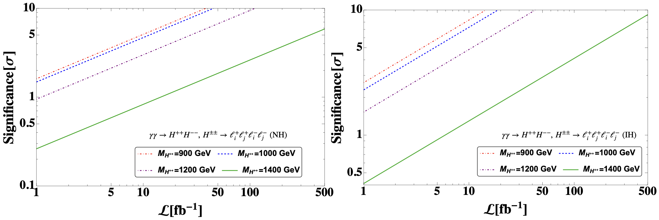
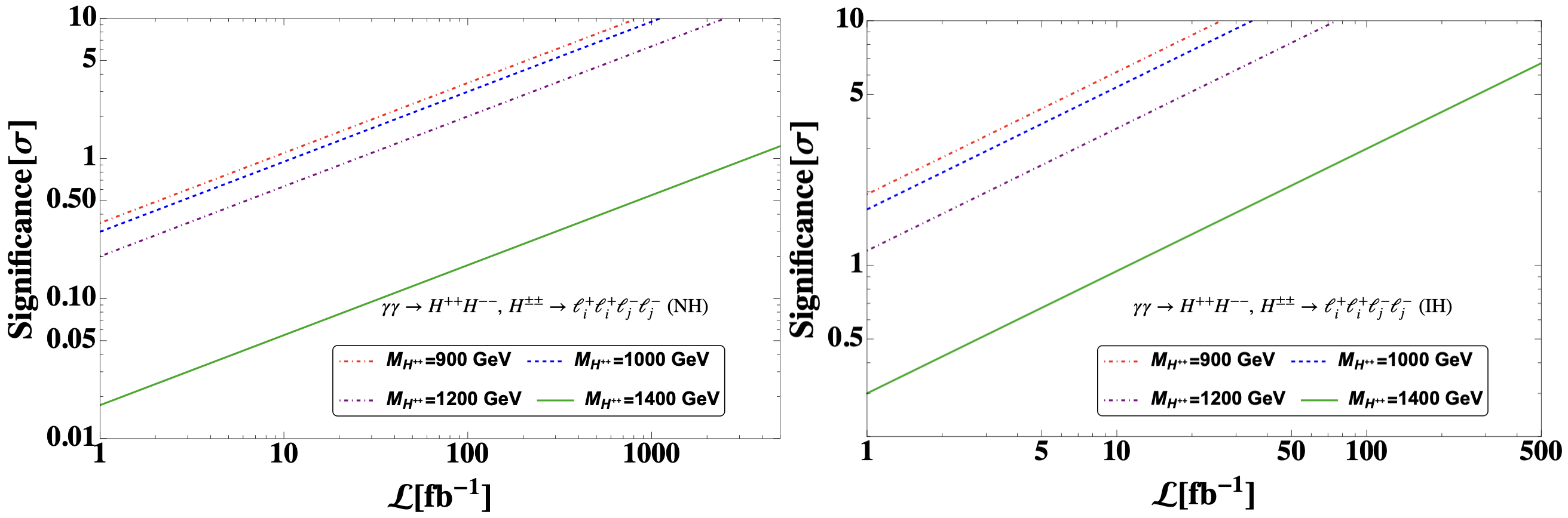
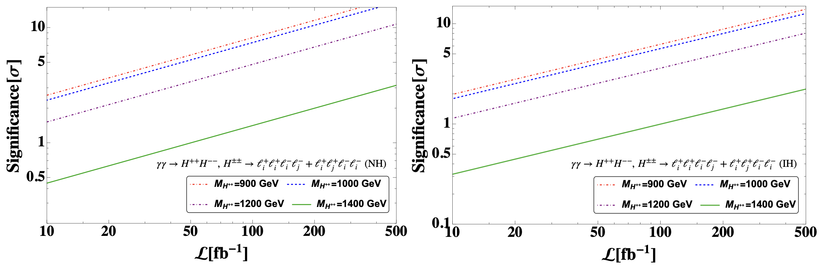
Figure 24: Significance of different final sates from $\gamma\gamma\to H^{++}H^{--}$ process at $\sqrt{s}=3$ TeV as a function of integrated luminosity.

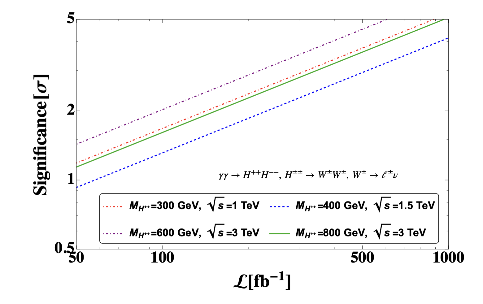
Figure 25: Significance of different final sates from $\gamma\gamma\to H^{++}H^{--}$ process at different $\sqrt{s}$ as a function of integrated luminosity.

IV.3 Different signatures from triplet fermions

We study the production of triplet fermion at the $e^{-}\gamma$ collider. The triplet fermion has neutral and charged multiplets. The lower limit on the triplet fermion mass form the LHC is nearly 1 TeV. As a result we consider $M_{\Sigma}\geq 1.2$ TeV and center of mass energy of $e^{-}\gamma$ collider as $3$ TeV. The dominant decay mode of the neutral multiplet is $W^{\mp}\ell$ and the second dominant mode of the charged multiplet is $Z\ell$. Due to the heavy triplet fermion mass under consideration, these $W$ and $Z$ bosons will be boosted and produce fat-jets. In this scenario we consider two different aspects in the following:

IV.3.1 SSDL mode

We first consider the $W^{-}\Sigma^{0}$ case where $W^{-}$ decays leptonically and $\Sigma^{0}$ decays into the dominant mode $e^{-}W^{+}$ where $W^{+}$ decays hadronically. In this analysis we consider a heavy triplet $M_{\Sigma}\geq 1.2$ TeV. As a result $W^{+}$ from the $\Sigma^{0}$ decay can be boosted so that the hadronic jets could be collimated to produce a boosted object called fat-jet $(J)$. The fat jet topology is a very powerful tool to significantly reduce the SM backgrounds. In our analysis the jets are reconstructed by Cambridge-Achen algorithm [259, 260] implemented in Fastjet [261, 262] package with the radius parameter as $R=0.8$. Hence we consider SSDL$+J$ signature in association with missing momentum. Again as in the case of Type-I seesaw we have two possibilities such as SSSF and SSDF depending on the flavour of $\ell^{-}$ coming from the associated $W^{-}$ decay. Hence we consider both the SSSF and SSDF signals with a fet-jet in association with missing momentum which can be useful to probe the Majorana nature of $\Sigma^{0}$. The corresponding Feynman diagram is given in Fig. 26.

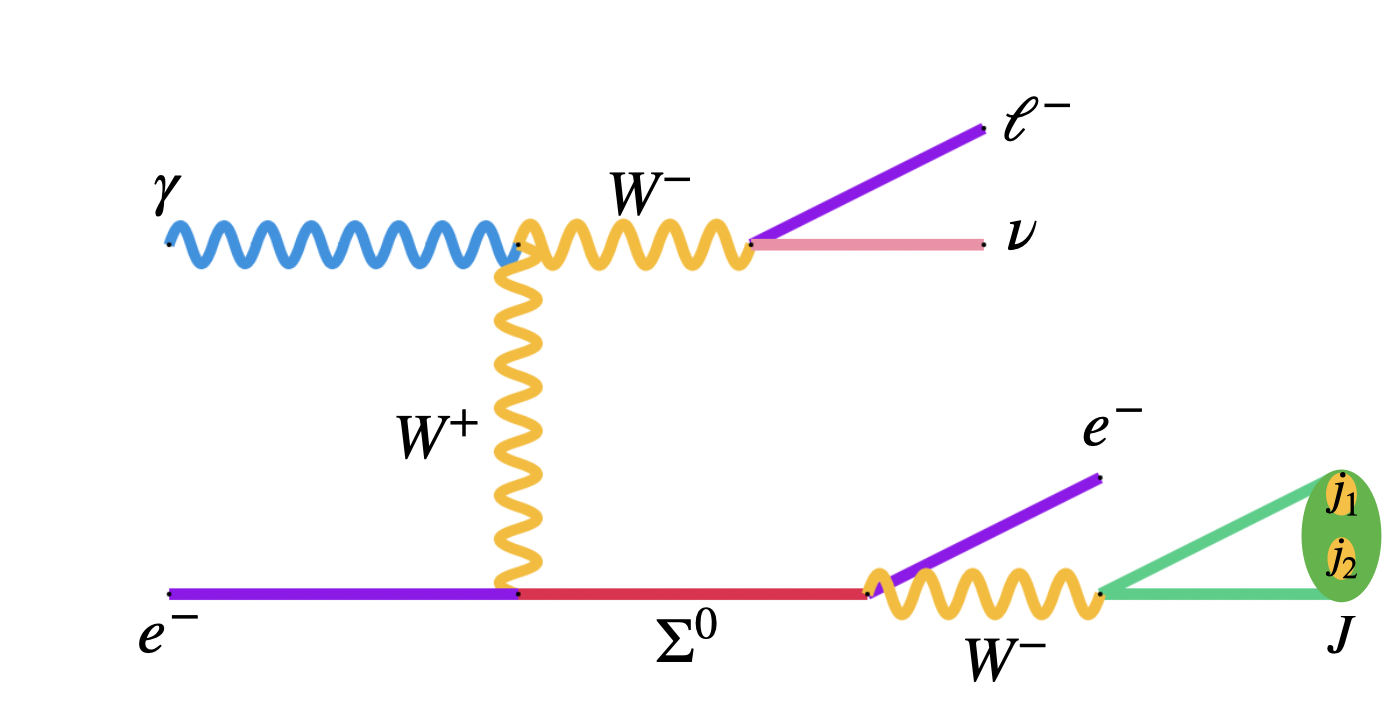
Figure 26: SSDL+ J final state in association with missing momentum at $e^{-}\gamma$ collider where $\ell^{-}=e^{-},\mu^{-}$. There is an additional $s$-channel process giving same final state which has been added in the analysis but not shown here.

In Fig. 27, we show the distributions of fat-jet transverse momentum $(p_{T}^{J})$, transverse momenta of the leptons $(p_{T}^{\ell_{1,2}})$, fat-jet mass $(m_{J})$, the polar angles of the leptons $(\cos\theta_{\ell_{1,2}})$ of the signal and corresponding backgrounds at $\sqrt{s}=3$ TeV. In view of these distributions we use the following cuts for the signal and generic background:

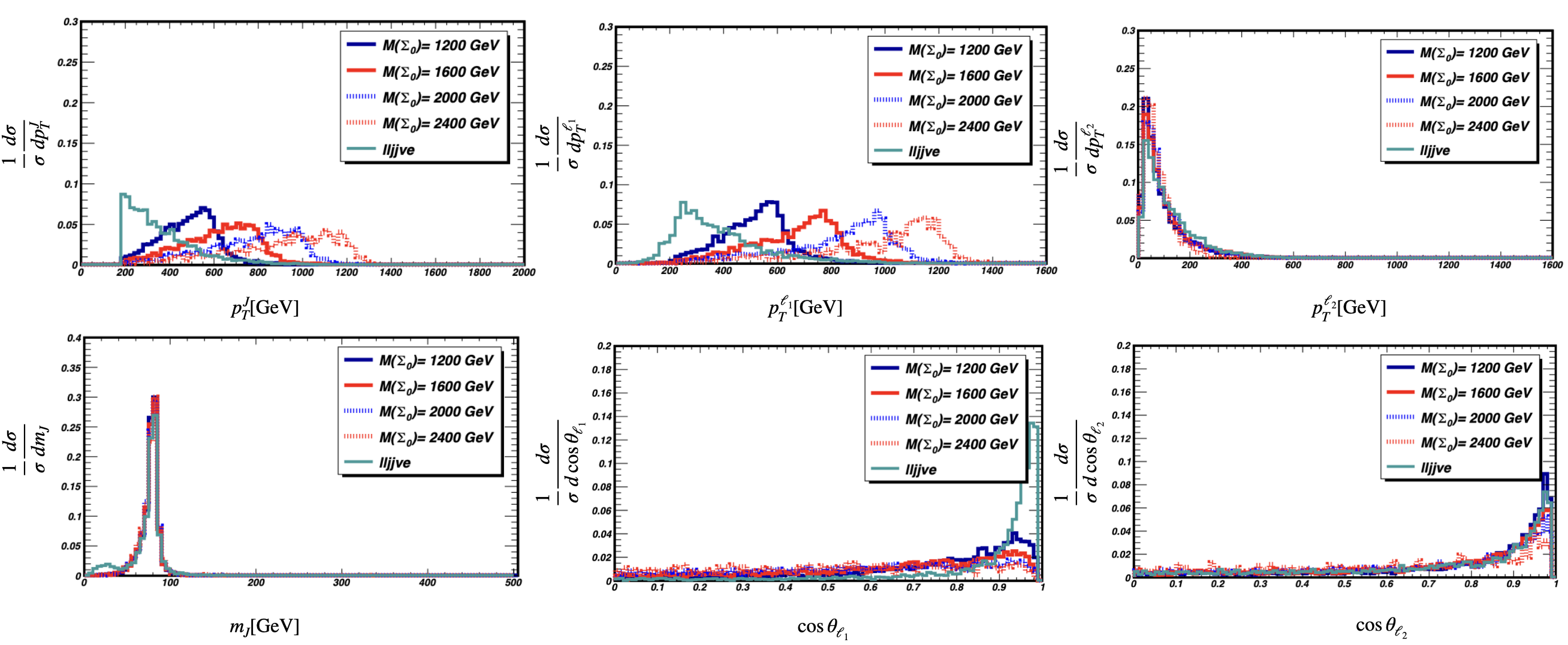
Figure 27: The distributions of different kinematic variables from the SSDL signal from type-III seesaw and corresponding generic background from $e^{-}\gamma$ collider at $\sqrt{s}=$3 TeV.

• The events selected with at least one fat-jets $(J)$ and leptons $(\ell=e,\mu)$ having transverse momenta $p_{T}^{J}>400$ GeV, $p_{T}^{\ell_{1},\rm leading}>400$ GeV and $p_{T}^{\ell_{2},\rm trailing}>10$ GeV respectively for the neutral component of the triplet fermion with mass $M_{\Sigma^{0}}=1200$ GeV, 1400 GeV, 1600 GeV and 1800 GeV respectively. For $M_{\Sigma^{0}}=2000$ GeV, 2200 GeV and 2400 GeV, the cuts are $p_{T}^{J}>600$ GeV, $p_{T}^{\ell_{1},\rm leading}>600$ GeV and $p_{T}^{\ell_{2},\rm trailing}>10$ GeV respectively.

• The jet mass $(m_{J})$ of the fat-jet is considered to be within 60 GeV $<m_{J}<$ 100 GeV.

• We reconstruct $\Sigma^{0}$ considering the electron and fat-jet system $(e^{-}J)$ and using the invariant mass cut $M_{\Sigma^{0}}-40$ GeV $<m_{\ell J}<M_{\Sigma^{0}}+40$ GeV where $M_{\Sigma^{0}}$ is the mass of the neutral component of the triplet fermion.

• The cosine of the polar angle of the leptons are considered to be $\cos\theta_{l_{1,\rm leading}}<0.92$ and $\cos\theta_{l_{2,\rm trailing}}<0.9$ respectively.

The signal normalized by the square of the mixing and corresponding background cross sections for the SSDL final state at $\sqrt{s}=$3 TeV are given in Tab. 17.

$\sqrt{s}$ (TeV)	$M_{\Sigma}$ (GeV)	Signal		Background
		before cuts (fb)	after cuts (fb)	before cuts (fb)	after cuts (fb)
	1200	2716.82	312.4	95.8	0.204
	1400	2527.68	377.15	95.8	0.243
3	1600	2317.24	394.13	95.8	0.252
	1800	2068.63	380.31	95.8	0.371
	2000	1763.19	711.1	95.8	0.128
	2200	1386.45	273.5	95.8	0.102
	2400	939.3	204.43	95.82	0.068

Table 17: Cross sections of the signal (normalized by $|V_{e\Sigma}|^{2}$) and generic background before and after cuts for $e^{-}\gamma$ collider at $\sqrt{s}=$3 TeV for the SSDL final state.

IV.3.2 Trilepton mode

The charged multiplets of the triplet fermion can also be produced at the $e^{-}\gamma$ collider in association with $Z$ boson. $\Sigma^{-}$ decays into $e^{-}Z$ followed by the hadronic decay mode of the $Z$ boson. Due to the heavy mass of the triplet fermion after the recent LHC limits we consider $M_{\Sigma}\geq 1$ TeV hence it can produce a boosted $Z$ boson which can produce a fat-jet after the hadronic decay which could have a unique feature. The associated $Z$ boson decays into a pair of charged leptons. Hence we finally observe a trilepton plus fat-jet signal which could be an interesting signature at the $e^{-}\gamma$ colliders. In addition to this mode another interesting channel could be the $\Sigma^{-}h$ mode where $h$ can decay into b-jets dominantly followed by the $\Sigma^{-}\to e^{-}J$ mode from the charged multiplet of the triplet fermion. However, in this article we finally concentrate on the gauge boson associated triplet production processes not including the Higgs associated channel in further consideration. The corresponding Feynman diagram is given in Fig. 28.

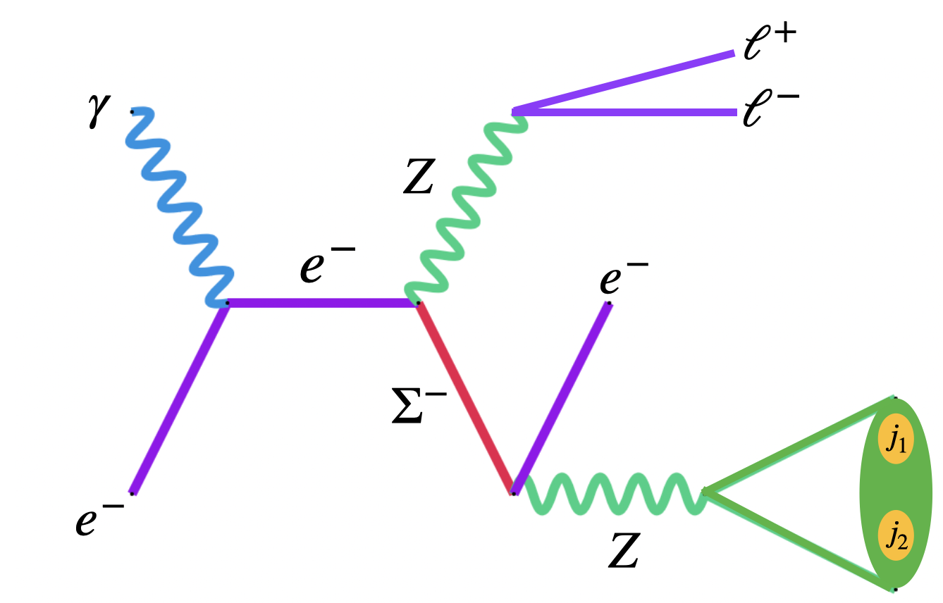
Figure 28: Feynman diagram for the process $e^{-}\gamma\to e^{-}\ell^{+}\ell^{-}+J$. There is an additional $t$-channel process giving same final state which has been added in the analysis but not shown here.

Generating the trilepton events with jets we show the distributions of fat-jet transverse momentum $(p_{T}^{J})$, transverse momenta of the leptons $(p_{T}^{\ell_{1,2,3}})$, fat-jet mass $(m_{J})$, the polar angles of the leptons $(\cos\theta_{\ell_{1,2,3}})$ of the signal and corresponding backgrounds in Fig. 29.

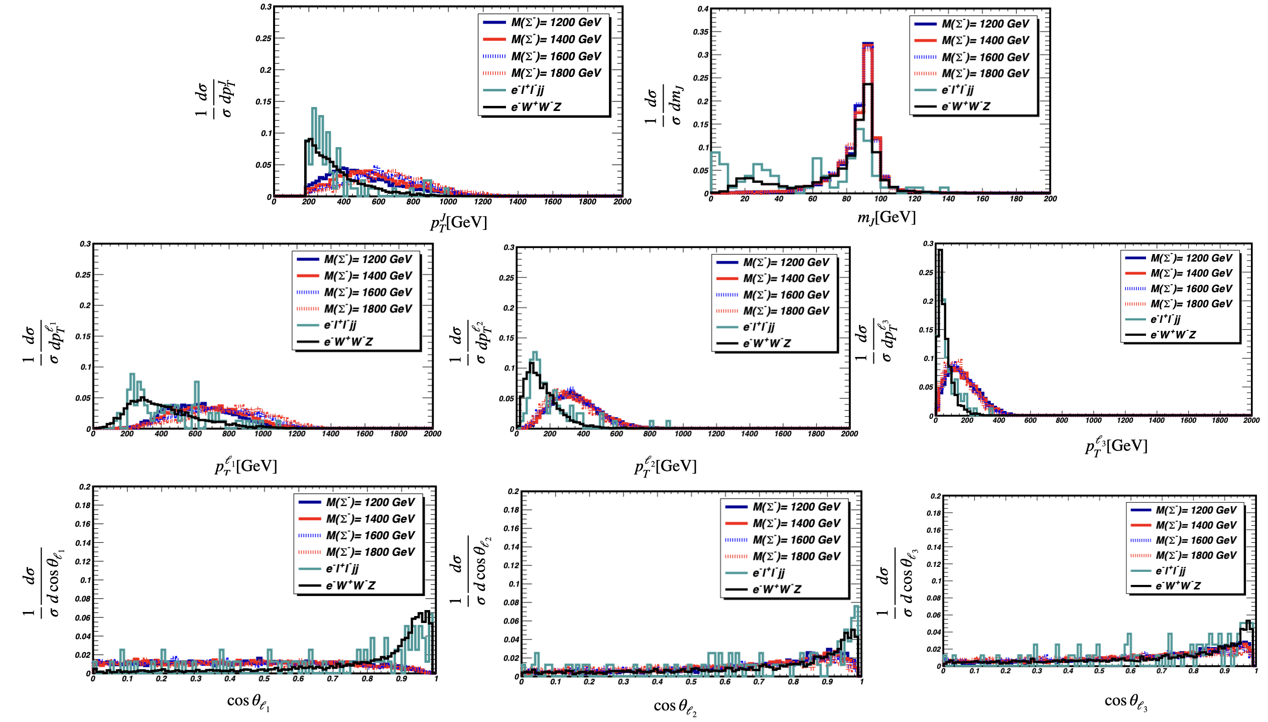
Figure 29: The distributions of different kinematic variables from the trilepton plus fat-jet signal from type-III seesaw and corresponding backgrounds from $e^{-}\gamma$ collider at $\sqrt{s}=$3 TeV.

In view of these distributions we use the following cuts to generate trilepton plus fat-jet events for the signal and generic background:

• The events selected with at least one fat-jet $(J)$ and three leptons having transverse momenta $p_{T}^{J}>300$ GeV, $p_{T}^{\ell_{1},\rm leading}>400$ GeV, $p_{T}^{\ell_{2},\rm trailing}>150$ GeV and $p_{T}^{\ell_{3},\rm trailing}>75$ GeV respectively for $M_{\Sigma}^{-}=1200$ GeV, 1400 GeV, 1600 GeV and 1800 GeV respectively.

• The jet mass $(m_{J})$ of the fat-jet is considered to be within 60 GeV $<m_{J}<$ 100 GeV.

• We reconstruct $\Sigma^{-}$ considering the electron and fat-jet system $(e^{-}J)$ and using the invariant mass cut $M_{\Sigma^{-}}-40$ GeV $<m_{\ell J}<M_{\Sigma^{-}}+40$ GeV.

• The cosine of the polar angle of the leptons are considered to be $\cos\theta_{l_{1,\rm leading}}<0.9$, $\cos\theta_{l_{2,\rm trailing}}<0.92$ and $\cos\theta_{l_{3,\rm trailing}}<0.94$ respectively.

The signal normalized by the square of the mixing and corresponding background cross sections for the trilepton plus fat-jet final state at $\sqrt{s}=$3 TeV are given in Tab. 18.

$\sqrt{s}$ (TeV)	$M_{\Sigma}$ (GeV)	Signal		Background
		before cuts (fb)	after cuts (fb)	before cuts (fb)	after cuts (fb)
	1200	24.67	3.63		-
					0.0014
	1400	21.23	5.11		-
					0.000741
3	1600	16.82	4.06	$e\ell\ell jj:0.491$	-
				$eWWZ:$1.353	0.00115
	1800	12.1	2.73		-
					0.00017

Table 18: Cross sections of the signal $e^{-}\gamma\to e^{-}\ell^{+}\ell^{-}+J$ (normalized by $|V_{e\Sigma}|^{2}$) and generic background before and after cuts for $e^{-}\gamma$ collider at $\sqrt{s}=$3 TeV. In the background column ‘-’ stands for extremely low cross section of the background $e\ell\ell jj$ compared to $eWWZ$.

IV.3.3 Limits on the mixing angle

For both the case of SSDL$+J$ and $e^{-}\ell^{+}\ell^{-}+J$, studying the signal $(S)$ and the corresponding backgrounds $(B)$ we estimate the 2-$\sigma$ limits on the mixing using Eq. 89 taking 5 ab^-1 of integrated luminosity as a benchmark. The limits coming from SSDL$+J$ and $e^{-}\ell^{+}\ell^{-}+J$ are represented by the thick blue and dashed blue line, respectively in Fig. 30. We compare the results with the limits from EWPD for electron $(V_{e\Sigma}=0.019)$ and universal EWPD $(V_{e\Sigma}=0.016)$ respectively from [235]. We find that the 2-$\sigma$ bound on the mixing for the SSDL signal can reach $\mathcal{O}(10^{-5})$ for $M_{\Sigma}=2$ TeV which is well below the expected limits. The 2-$\sigma$ limit on the mixing from the trilepton plus fat-jet signal can reach up to $2.2\times 10^{-4}$ for $M_{\Sigma}=1.475$ TeV which is slightly stronger than the EWPD-U limit. We find that the limits almost remain flat through out the mass range we consider apart from some heavy masses where fat-jet signatures become stronger for the signal over the backgrounds. We do not probe the energy threshold because cross section sharply falls near that region which may provide comparatively weaker bounds on the mixing.

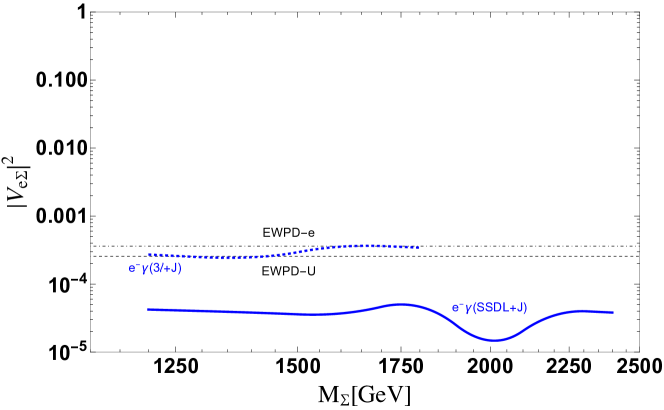
Figure 30: $2\sigma$ limits on the mixing angle from SSDL+J in association with missing momentum (thick, blue) and $3\ell+J$ final state (dashed, blue) at $e^{-}\gamma$ collider with $\sqrt{s}=3$ TeV at 5 ab^-1 luminosity. We compare the results with the limits from EWPD for electron (black dot-dashed) and universal EWPD (black dashed).

V Discussions and conclusions

In this paper we study three types of electroweak scale seesaw scenarios at electron photon and photon photon colliders at different center of mass energies. We have systemically calculated the cross sections of different production modes of the BSM particles at these colliders averaging over photon spectrum for fixed $\sqrt{s}$ as a function of the corresponding BSM particle mass. First we consider the production of a heavy Majorana neutrinos from the type-I seesaw scenario at the electron photon collider in association with $W$ boson. From this channel we study $e^{\pm}+4j$ scenario where the heavy neutrino dominantly decays to $W^{\mp}e^{\pm}$, followed by the hadronic decay of W bosons produced in this channel. In addition to that we consider the leptonic decay of the associated $W$ boson so that SSDL and OSDL modes could be obtained. Considering these final states in association with two jets from the hadronic decay of the $W$ boson coming from the heavy neutrino we estimate the limits on the light-heavy mixing. Hence combining SSDL mode with $e^{\pm}+4j$ and OSDL mode with $e^{\pm}+4j$ we estimate limits on the mixing angle separately for comparison at $2\sigma$ significance. For completeness we compare the limits with the existing bounds and prospective limits at electron positron colliders at different center of mass energies. Depending on the center of mass energy, heavy neutrino mass and the choice of the final state signal, the limits on the light-heavy mixing obtained from electron photon colliders could be stronger compare to existing limits. The obtained limits are stronger than the limits obtained from the eletroweak precision study. Second we consider the type-II seesaw scenario where we produce doubly charged scalar at photon photon collider studying a variety of multilepton modes. Studying the signals and SM backgrounds we find that signals with 5$\sigma$ significance could be obtained at 3 TeV photon photon collider where the triplet scalar masses around 1 TeV. Like the singlet fermion we have studied triplet fermion production in electron photon collider from the type-III seesaw scenario as the third case. In this case we consider 3 TeV collider as the triplet mass is greater than 1.2 TeV due to the current LHC limit. We study SSDL mode from the neutral multiplet and trilepton mode from the charged multiplet of the triplet fermion in association with fat-jet. Studying the signal and SM backgrounds we estimate limits on the light-heavy mixings and find stronger bounds compared to those obtained from the eletroweak precision measurements. Finally we mention that a systematic study involving multivariate analysis may improve these results. When electron positron collider will be built in future, unique opportunities of constructing electron photon and photon photon colliders will be possible where one can test electroweak scale seesaw scenarios. This will help to fix neutrino mass generation mechanism. In addition to that possible studies on Majorana or Dirac nature of neutrinos could also be possible.
Finally we would like to stress that in our study we have used the cut-based analyses where the cuts do depend on the mass of the heavy degrees of freedom. This search strategy is always less efficient than a “bump-hunting" algorithm or a boosted decision tree (BDT) based on general kinematic variables which are not based on search mass priors. Also we would like to again mention that if one consider polarized beam, the bound might be weaker compare to what we obtained.

Appendix A Photon PDF

⬇

1 ! bcompton(y,epol,apol) described below is the function which gives the energy spectrum of the photon coming from Compton back-scattering. ! y is the ratio between photon energy and electron energy. epol and apol are the electron and photon polarization.

2 ! The bcompton(y,epol,apol) function described below is written based on the paper hep-ex/0108012 can be added at line number 101 of PhotonFlux.f file in Madgraph.

3

4 real*8 function bcompton(y,epol,apol)

5 real*8 y,epol,apol

6 real*8 x,Dx,lee,laa,ymax,r,f

7 data x/2.24034d0/

8

9 lee=0.0d0*epol

10 laa=apol

11

12 Dx= (1d0-4d0/x-8d0/x**2)*dlog(1d0+x)+0.5d0+8d0/x-0.5d0/(1d0+x)**2

13 & +2d0*lee*laa*( (1d0+2d0/x)*dlog(1d0+x)-2.5d0+1d0/(1d0+x)

14 & -0.5/(1d0+x)**2 )

15

16 ymax=x/(1d0+x)

17 if (y.le.ymax) then

18 r=y/x/(1d0-y)

19 f=( 1d0/(1d0-y) +1d0-y -4d0*r*(1d0-r)

20 & -2d0*lee*laa*r*x*(2d0*r-1d0)*(2d0-y) ) /Dx

21 else

22 f=0d0

23 endif

24 bcompton = f

25 !write(1,*)y,f

26 end

- [1] Particle Data Group Collaboration, P. A. Zyla et al., “Review of Particle Physics,” PTEP 2020 no. 8, (2020) 083C01.
- [2] S. Weinberg, “Baryon and Lepton Nonconserving Processes,” Phys. Rev. Lett. 43 (1979) 1566–1570.
- [3] J. Schechter and J. W. F. Valle, “Neutrino Masses in SU(2) x U(1) Theories,” Phys. Rev. D 22 (1980) 2227.
- [4] P. Minkowski, “ at a Rate of One Out of Muon Decays?,” Phys. Lett. B 67 (1977) 421–428.
- [5] M. Gell-Mann, P. Ramond, and R. Slansky, “Complex Spinors and Unified Theories,” Conf. Proc. C 790927 (1979) 315–321, arXiv:1306.4669 [hep-th].
- [6] T. Yanagida, “Horizontal gauge symmetry and masses of neutrinos,” Conf. Proc. C 7902131 (1979) 95–99.
- [7] O. Sawada and A. Sugamoto, eds., Proceedings: Workshop on the Unified Theories and the Baryon Number in the Universe: Tsukuba, Japan, February 13-14, 1979. Natl.Lab.High Energy Phys., Tsukuba, Japan, 1979.
- [8] R. N. Mohapatra and G. Senjanovic, “Neutrino Mass and Spontaneous Parity Nonconservation,” Phys. Rev. Lett. 44 (1980) 912.
- [9] K. N. Abazajian et al., “Light Sterile Neutrinos: A White Paper,” arXiv:1204.5379 [hep-ph].
- [10] BOREXINO Collaboration, G. Bellini et al., “Neutrinos from the primary proton–proton fusion process in the Sun,” Nature 512 no. 7515, (2014) 383–386.
- [11] MiniBooNE Collaboration, A. A. Aguilar-Arevalo et al., “Updated MiniBooNE neutrino oscillation results with increased data and new background studies,” Phys. Rev. D 103 no. 5, (2021) 052002, arXiv:2006.16883 [hep-ex].
- [12] P. B. Denton, “Sterile Neutrino Searches with MicroBooNE: Electron Neutrino Disappearance,” arXiv:2111.05793 [hep-ph].
- [13] P. D. Bolton, F. F. Deppisch, and P. S. Bhupal Dev, “Neutrinoless double beta decay versus other probes of heavy sterile neutrinos,” JHEP 03 (2020) 170, arXiv:1912.03058 [hep-ph].
- [14] P. A. Machado, O. Palamara, and D. W. Schmitz, “The Short-Baseline Neutrino Program at Fermilab,” Ann. Rev. Nucl. Part. Sci. 69 (2019) 363–387, arXiv:1903.04608 [hep-ex].
- [15] MicroBooNE Collaboration, P. Abratenko et al., “Search for Neutrino-Induced Neutral Current Radiative Decay in MicroBooNE and a First Test of the MiniBooNE Low Energy Excess Under a Single-Photon Hypothesis,” arXiv:2110.00409 [hep-ex].
- [16] C. A. Argüelles, K. Farrag, T. Katori, R. Khandelwal, S. Mandalia, and J. Salvado, “Sterile neutrinos in astrophysical neutrino flavor,” JCAP 02 (2020) 015, arXiv:1909.05341 [hep-ph].
- [17] B. Dasgupta and J. Kopp, “Sterile Neutrinos,” Phys. Rept. 928 (2021) 63, arXiv:2106.05913 [hep-ph].
- [18] K. Jodłowski and S. Trojanowski, “Neutrino beam-dump experiment with FASER at the LHC,” JHEP 05 (2021) 191, arXiv:2011.04751 [hep-ph].
- [19] P. Bakhti, Y. Farzan, and S. Pascoli, “Discovery potential of FASER with contained vertex and through-going events,” JHEP 04 (2021) 075, arXiv:2010.16312 [hep-ph].
- [20] Y. Jho, J. Kim, P. Ko, and S. C. Park, “Search for sterile neutrino with light gauge interactions: recasting collider, beam-dump, and neutrino telescope searches,” arXiv:2008.12598 [hep-ph].
- [21] P. Ballett, T. Boschi, and S. Pascoli, “Heavy Neutral Leptons from low-scale seesaws at the DUNE Near Detector,” JHEP 03 (2020) 111, arXiv:1905.00284 [hep-ph].
- [22] S. Carbajal and A. M. Gago, “Indirect search of Heavy Neutral Leptons using the DUNE Near Detector,” arXiv:2202.09217 [hep-ph].
- [23] G. Cvetic, C. Dib, and C. S. Kim, “Probing Majorana neutrinos in rare decays,” JHEP 06 (2012) 149, arXiv:1203.0573 [hep-ph].
- [24] G. Cvetič, C. S. Kim, and J. Zamora-Saá, “CP violation in lepton number violating semihadronic decays of ,” Phys. Rev. D 89 no. 9, (2014) 093012, arXiv:1403.2555 [hep-ph].
- [25] C. Dib and C. S. Kim, “Remarks on the lifetime of sterile neutrinos and the effect on detection of rare meson decays ,” Phys. Rev. D 89 no. 7, (2014) 077301, arXiv:1403.1985 [hep-ph].
- [26] G. Cvetic, C. S. Kim, R. Kogerler, and J. Zamora-Saa, “Oscillation of heavy sterile neutrino in decay of ,” Phys. Rev. D 92 (2015) 013015, arXiv:1505.04749 [hep-ph].
- [27] S. Mandal and N. Sinha, “Favoured Decay modes to search for a Majorana neutrino,” Phys. Rev. D 94 no. 3, (2016) 033001, arXiv:1602.09112 [hep-ph].
- [28] S. Mandal, M. Mitra, and N. Sinha, “Constraining the right-handed gauge boson mass from lepton number violating meson decays in a low scale left-right model,” Phys. Rev. D 96 no. 3, (2017) 035023, arXiv:1705.01932 [hep-ph].
- [29] C. O. Dib, C. S. Kim, and K. Wang, “Signatures of Dirac and Majorana sterile neutrinos in trilepton events at the LHC,” Phys. Rev. D 95 no. 11, (2017) 115020, arXiv:1703.01934 [hep-ph].
- [30] G. Cvetic and C. S. Kim, “Sensitivity limits on heavy-light mixing from lepton number violating meson decays,” Phys. Rev. D 96 no. 3, (2017) 035025, arXiv:1705.09403 [hep-ph]. [Erratum: Phys.Rev.D 102, 019903 (2020), Erratum: Phys.Rev.D 102, 039902 (2020)].
- [31] E. J. Chun, A. Das, S. Mandal, M. Mitra, and N. Sinha, “Sensitivity of Lepton Number Violating Meson Decays in Different Experiments,” Phys. Rev. D 100 no. 9, (2019) 095022, arXiv:1908.09562 [hep-ph].
- [32] S. Tapia, M. Vidal-Bravo, and J. Zamora-Saa, “Discovering heavy neutrino oscillations in rare Bc meson decays at HL-LHCb,” Phys. Rev. D 105 no. 3, (2022) 035003, arXiv:2109.06027 [hep-ph].
- [33] J.-L. Tastet, E. Goudzovski, I. Timiryasov, and O. Ruchayskiy, “Projected NA62 sensitivity to heavy neutral lepton production in K+→0e+N decays,” Phys. Rev. D 104 no. 5, (2021) 055005, arXiv:2008.11654 [hep-ph].
- [34] A. Abada, D. Bečirević, O. Sumensari, C. Weiland, and R. Zukanovich Funchal, “Sterile neutrinos facing kaon physics experiments,” Phys. Rev. D 95 no. 7, (2017) 075023, arXiv:1612.04737 [hep-ph].
- [35] Y.-S. Tsai, “Decay Correlations of Heavy Leptons in ,” Phys. Rev. D 4 (1971) 2821. [Erratum: Phys.Rev.D 13, 771 (1976)].
- [36] M. Gourdin and X.-Y. Pham, “Study of Electron Type Neutral Heavy Lepton in Electron - Positron Reactions. 1. Production,” Nucl. Phys. B 164 (1980) 387–398.
- [37] M. Gourdin and X.-Y. Pham, “STUDY OF ELECTRON TYPE NEUTRAL HEAVY LEPTON IN ELECTRON - POSITRON REACTIONS. 2. LEPTONIC DECAY,” Nucl. Phys. B 164 (1980) 399–412.
- [38] S. T. Petcov, “Possible Signature for Production of Majorana Particles in and Collisions,” Phys. Lett. B 139 (1984) 421–426.
- [39] J. Maalampi, K. Mursula, and R. Vuopionpera, “Heavy neutrinos in e+ e- collisions,” Nucl. Phys. B 372 (1992) 23–43.
- [40] W. Buchmuller and C. Greub, “Right-handed currents and heavy neutrinos in high-energy and scattering,” Nucl. Phys. B 381 (1992) 109–128.
- [41] T. Asaka and M. Shaposhnikov, “The MSM, dark matter and baryon asymmetry of the universe,” Phys. Lett. B 620 (2005) 17–26, arXiv:hep-ph/0505013.
- [42] T. Han and B. Zhang, “Signatures for Majorana neutrinos at hadron colliders,” Phys. Rev. Lett. 97 (2006) 171804, arXiv:hep-ph/0604064.
- [43] D. Gorbunov and M. Shaposhnikov, “How to find neutral leptons of the MSM?,” JHEP 10 (2007) 015, arXiv:0705.1729 [hep-ph]. [Erratum: JHEP 11, 101 (2013)].
- [44] F. del Aguila and J. A. Aguilar-Saavedra, “Distinguishing seesaw models at LHC with multi-lepton signals,” Nucl. Phys. B 813 (2009) 22–90, arXiv:0808.2468 [hep-ph].
- [45] M. Mitra, G. Senjanovic, and F. Vissani, “Neutrinoless Double Beta Decay and Heavy Sterile Neutrinos,” Nucl. Phys. B 856 (2012) 26–73, arXiv:1108.0004 [hep-ph].
- [46] A. Das and N. Okada, “Inverse seesaw neutrino signatures at the LHC and ILC,” Phys. Rev. D 88 (2013) 113001, arXiv:1207.3734 [hep-ph].
- [47] P. S. Bhupal Dev, R. Franceschini, and R. N. Mohapatra, “Bounds on TeV Seesaw Models from LHC Higgs Data,” Phys. Rev. D 86 (2012) 093010, arXiv:1207.2756 [hep-ph].
- [48] P. S. B. Dev, A. Pilaftsis, and U.-k. Yang, “New Production Mechanism for Heavy Neutrinos at the LHC,” Phys. Rev. Lett. 112 no. 8, (2014) 081801, arXiv:1308.2209 [hep-ph].
- [49] A. Das, P. S. Bhupal Dev, and N. Okada, “Direct bounds on electroweak scale pseudo-Dirac neutrinos from TeV LHC data,” Phys. Lett. B 735 (2014) 364–370, arXiv:1405.0177 [hep-ph].
- [50] A. Das and N. Okada, “Improved bounds on the heavy neutrino productions at the LHC,” Phys. Rev. D 93 no. 3, (2016) 033003, arXiv:1510.04790 [hep-ph].
- [51] S. Antusch, E. Cazzato, and O. Fischer, “Higgs production from sterile neutrinos at future lepton colliders,” JHEP 04 (2016) 189, arXiv:1512.06035 [hep-ph].
- [52] A. Das, P. Konar, and S. Majhi, “Production of Heavy neutrino in next-to-leading order QCD at the LHC and beyond,” JHEP 06 (2016) 019, arXiv:1604.00608 [hep-ph].
- [53] A. Das, P. Konar, and A. Thalapillil, “Jet substructure shedding light on heavy Majorana neutrinos at the LHC,” JHEP 02 (2018) 083, arXiv:1709.09712 [hep-ph].
- [54] A. Bhardwaj, A. Das, P. Konar, and A. Thalapillil, “Looking for Minimal Inverse Seesaw scenarios at the LHC with Jet Substructure Techniques,” J. Phys. G 47 no. 7, (2020) 075002, arXiv:1801.00797 [hep-ph].
- [55] S. Antusch, E. Cazzato, O. Fischer, A. Hammad, and K. Wang, “Lepton Flavor Violating Dilepton Dijet Signatures from Sterile Neutrinos at Proton Colliders,” JHEP 10 (2018) 067, arXiv:1805.11400 [hep-ph].
- [56] E. Arganda, M. J. Herrero, X. Marcano, and C. Weiland, “Exotic jj events from heavy ISS neutrinos at the LHC,” Phys. Lett. B 752 (2016) 46–50, arXiv:1508.05074 [hep-ph].
- [57] A. Das, P. S. B. Dev, and C. S. Kim, “Constraining Sterile Neutrinos from Precision Higgs Data,” Phys. Rev. D 95 no. 11, (2017) 115013, arXiv:1704.00880 [hep-ph].
- [58] A. Das, Y. Gao, and T. Kamon, “Heavy neutrino search via semileptonic Higgs decay at the LHC,” Eur. Phys. J. C 79 no. 5, (2019) 424, arXiv:1704.00881 [hep-ph].
- [59] S. Chakraborty, M. Mitra, and S. Shil, “Fat Jet Signature of a Heavy Neutrino at Lepton Collider,” Phys. Rev. D 100 no. 1, (2019) 015012, arXiv:1810.08970 [hep-ph].
- [60] A. Das, S. Jana, S. Mandal, and S. Nandi, “Probing right handed neutrinos at the LHeC and lepton colliders using fat jet signatures,” Phys. Rev. D 99 no. 5, (2019) 055030, arXiv:1811.04291 [hep-ph].
- [61] J. Liu, Z. Liu, L.-T. Wang, and X.-P. Wang, “Enhancing Sensitivities to Long-lived Particles with High Granularity Calorimeters at the LHC,” JHEP 11 (2020) 066, arXiv:2005.10836 [hep-ph].
- [62] A. Das and N. Okada, “Bounds on heavy Majorana neutrinos in type-I seesaw and implications for collider searches,” Phys. Lett. B 774 (2017) 32–40, arXiv:1702.04668 [hep-ph].
- [63] J. Liu, Z. Liu, L.-T. Wang, and X.-P. Wang, “Seeking for sterile neutrinos with displaced leptons at the LHC,” JHEP 07 (2019) 159, arXiv:1904.01020 [hep-ph].
- [64] S. Mondal and S. K. Rai, “Probing the Heavy Neutrinos of Inverse Seesaw Model at the LHeC,” Phys. Rev. D 94 no. 3, (2016) 033008, arXiv:1605.04508 [hep-ph].
- [65] J. C. Helo, M. Hirsch, and Z. S. Wang, “Heavy neutral fermions at the high-luminosity LHC,” JHEP 07 (2018) 056, arXiv:1803.02212 [hep-ph].
- [66] M. Drewes, “The Phenomenology of Right Handed Neutrinos,” Int. J. Mod. Phys. E 22 (2013) 1330019, arXiv:1303.6912 [hep-ph].
- [67] M. Drewes and J. Hajer, “Heavy Neutrinos in displaced vertex searches at the LHC and HL-LHC,” JHEP 02 (2020) 070, arXiv:1903.06100 [hep-ph].
- [68] M. Drewes, A. Giammanco, J. Hajer, and M. Lucente, “New long-lived particle searches in heavy-ion collisions at the LHC,” Phys. Rev. D 101 no. 5, (2020) 055002, arXiv:1905.09828 [hep-ph].
- [69] M. Hirsch and Z. S. Wang, “Heavy neutral leptons at ANUBIS,” Phys. Rev. D 101 no. 5, (2020) 055034, arXiv:2001.04750 [hep-ph].
- [70] Y. Gao and K. Wang, “Heavy Neutrino Searches via Same-sign Lepton Pairs at the Higgs Factory,” arXiv:2102.12826 [hep-ph].
- [71] A. Abada, C. Hati, X. Marcano, and A. M. Teixeira, “Interference effects in LNV and LFV semileptonic decays: the Majorana hypothesis,” JHEP 09 (2019) 017, arXiv:1904.05367 [hep-ph].
- [72] A. Abada, N. Bernal, M. Losada, and X. Marcano, “Inclusive Displaced Vertex Searches for Heavy Neutral Leptons at the LHC,” JHEP 01 (2019) 093, arXiv:1807.10024 [hep-ph].
- [73] A. Abada, A. Hernández-Cabezudo, and X. Marcano, “Beta and Neutrinoless Double Beta Decays with KeV Sterile Fermions,” JHEP 01 (2019) 041, arXiv:1807.01331 [hep-ph].
- [74] V. De Romeri, M. J. Herrero, X. Marcano, and F. Scarcella, “Lepton flavor violating Z decays: A promising window to low scale seesaw neutrinos,” Phys. Rev. D 95 no. 7, (2017) 075028, arXiv:1607.05257 [hep-ph].
- [75] A. Abada, V. De Romeri, M. Lucente, A. M. Teixeira, and T. Toma, “Effective Majorana mass matrix from tau and pseudoscalar meson lepton number violating decays,” JHEP 02 (2018) 169, arXiv:1712.03984 [hep-ph].
- [76] A. Abada, V. De Romeri, and A. M. Teixeira, “Impact of sterile neutrinos on nuclear-assisted cLFV processes,” JHEP 02 (2016) 083, arXiv:1510.06657 [hep-ph].
- [77] J.-L. Tastet, O. Ruchayskiy, and I. Timiryasov, “Reinterpreting the ATLAS bounds on heavy neutral leptons in a realistic neutrino oscillation model,” JHEP 12 (2021) 182, arXiv:2107.12980 [hep-ph].
- [78] K. Mękała, J. Reuter, and A. F. Żarnecki, “Heavy neutrinos at future linear e+e- colliders,” JHEP 06 (2022) 010, arXiv:2202.06703 [hep-ph].
- [79] F. del Aguila and J. A. Aguilar-Saavedra, “Electroweak scale seesaw and heavy Dirac neutrino signals at LHC,” Phys. Lett. B 672 (2009) 158–165, arXiv:0809.2096 [hep-ph].
- [80] F. del Aguila, J. A. Aguilar-Saavedra, and R. Pittau, “Heavy neutrino signals at large hadron colliders,” JHEP 10 (2007) 047, arXiv:hep-ph/0703261.
- [81] F. del Aguila and J. A. Aguilar-Saavedra, “l W nu production at CLIC: A Window to TeV scale non-decoupled neutrinos,” JHEP 05 (2005) 026, arXiv:hep-ph/0503026.
- [82] F. del Aguila, J. A. Aguilar-Saavedra, A. Martinez de la Ossa, and D. Meloni, “Flavor and polarisation in heavy neutrino production at e+ e- colliders,” Phys. Lett. B 613 (2005) 170–180, arXiv:hep-ph/0502189.
- [83] D. Atwood, S. Bar-Shalom, and A. Soni, “Neutrino masses, mixing and leptogenesis in a two Higgs doublet model ’for the third generation’,” Phys. Lett. B 635 (2006) 112–117, arXiv:hep-ph/0502234.
- [84] D. Atwood, S. Bar-Shalom, and A. Soni, “Seesaw induced electroweak scale, the hierarchy problem and sub-eV neutrino masses,” Eur. Phys. J. C 45 (2006) 219–225, arXiv:hep-ph/0408191.
- [85] F. del Aguila, S. Bar-Shalom, A. Soni, and J. Wudka, “Heavy Majorana Neutrinos in the Effective Lagrangian Description: Application to Hadron Colliders,” Phys. Lett. B 670 (2009) 399–402, arXiv:0806.0876 [hep-ph].
- [86] S. Bar-Shalom, G. Eilam, T. Han, and A. Soni, “Charged Higgs Boson Effects in the Production and Decay of a Heavy Majorana Neutrino at the CERN LHC,” Phys. Rev. D 77 (2008) 115019, arXiv:0803.2835 [hep-ph].
- [87] D. Atwood, S. Bar-Shalom, and A. Soni, “Signature of heavy Majorana neutrinos at a linear collider: Enhanced charged Higgs pair production,” Phys. Rev. D 76 (2007) 033004, arXiv:hep-ph/0701005.
- [88] S. Bar-Shalom, N. G. Deshpande, G. Eilam, J. Jiang, and A. Soni, “Majorana neutrinos and lepton-number-violating signals in top-quark and W-boson rare decays,” Phys. Lett. B 643 (2006) 342–347, arXiv:hep-ph/0608309.
- [89] G. Cottin, O. Fischer, S. Mandal, M. Mitra, and R. Padhan, “Displaced Neutrino Jets at the LHeC,” arXiv:2104.13578 [hep-ph].
- [90] G. Bélanger, S. Khan, R. Padhan, M. Mitra, and S. Shil, “Right handed neutrinos, TeV scale BSM neutral Higgs boson, and FIMP dark matter in an EFT framework,” Phys. Rev. D 104 no. 5, (2021) 055047, arXiv:2104.04373 [hep-ph].
- [91] G. Cottin, J. C. Helo, M. Hirsch, A. Titov, and Z. S. Wang, “Heavy neutral leptons in effective field theory and the high-luminosity LHC,” JHEP 09 (2021) 039, arXiv:2105.13851 [hep-ph].
- [92] A. Abada, P. Escribano, X. Marcano, and G. Piazza, “Collider searches for heavy neutral leptons: beyond simplified scenarios,” Eur. Phys. J. C 82 no. 11, (2022) 1030, arXiv:2208.13882 [hep-ph].
- [93] C. A. R, G. Cottin, J. C. Helo, and M. Hirsch, “Long-lived charged particles and multi-lepton signatures from neutrino mass models,” Phys. Rev. D 101 no. 9, (2020) 095033, arXiv:2003.11494 [hep-ph].
- [94] C. O. Dib, J. C. Helo, M. Nayak, N. A. Neill, A. Soffer, and J. Zamora-Saa, “Searching for a sterile neutrino that mixes predominantly with at factories,” Phys. Rev. D 101 no. 9, (2020) 093003, arXiv:1908.09719 [hep-ph].
- [95] G. Cottin, J. C. Helo, and M. Hirsch, “Displaced vertices as probes of sterile neutrino mixing at the LHC,” Phys. Rev. D 98 no. 3, (2018) 035012, arXiv:1806.05191 [hep-ph].
- [96] G. Cottin, J. C. Helo, and M. Hirsch, “Searches for light sterile neutrinos with multitrack displaced vertices,” Phys. Rev. D 97 no. 5, (2018) 055025, arXiv:1801.02734 [hep-ph].
- [97] D. Barducci, E. Bertuzzo, A. Caputo, P. Hernandez, and B. Mele, “The see-saw portal at future Higgs Factories,” JHEP 03 (2021) 117, arXiv:2011.04725 [hep-ph].
- [98] F. F. Deppisch, P. S. Bhupal Dev, and A. Pilaftsis, “Neutrinos and Collider Physics,” New J. Phys. 17 no. 7, (2015) 075019, arXiv:1502.06541 [hep-ph].
- [99] A. Das, “Searching for the minimal Seesaw models at the LHC and beyond,” Adv. High Energy Phys. 2018 (2018) 9785318, arXiv:1803.10940 [hep-ph].
- [100] P. Bandyopadhyay, A. Karan, and C. Sen, “Discerning Signatures of Seesaw Models and Complementarity of Leptonic Colliders,” arXiv:2011.04191 [hep-ph].
- [101] X.-G. He, S. Oh, J. Tandean, and C.-C. Wen, “Large Mixing of Light and Heavy Neutrinos in Seesaw Models and the LHC,” Phys. Rev. D 80 (2009) 073012, arXiv:0907.1607 [hep-ph].
- [102] K. Mękała, J. Reuter, and A. F. Żarnecki, “Optimal search reach for heavy neutral leptons at a muon collider,” Phys. Lett. B 841 (2023) 137945, arXiv:2301.02602 [hep-ph].
- [103] T. H. Kwok, L. Li, T. Liu, and A. Rock, “Searching for Heavy Neutral Leptons at A Future Muon Collider,” arXiv:2301.05177 [hep-ph].
- [104] P. Li, Z. Liu, and K.-F. Lyu, “Heavy neutral leptons at muon colliders,” JHEP 03 (2023) 231, arXiv:2301.07117 [hep-ph].
- [105] J. Schechter and J. W. F. Valle, “Neutrino Decay and Spontaneous Violation of Lepton Number,” Phys. Rev. D 25 (1982) 774.
- [106] M. Magg and C. Wetterich, “Neutrino Mass Problem and Gauge Hierarchy,” Phys. Lett. B 94 (1980) 61–64.
- [107] T. P. Cheng and L.-F. Li, “Neutrino Masses, Mixings and Oscillations in SU(2) x U(1) Models of Electroweak Interactions,” Phys. Rev. D 22 (1980) 2860.
- [108] G. Lazarides, Q. Shafi, and C. Wetterich, “Proton Lifetime and Fermion Masses in an SO(10) Model,” Nucl. Phys. B 181 (1981) 287–300.
- [109] R. N. Mohapatra and G. Senjanovic, “Neutrino Masses and Mixings in Gauge Models with Spontaneous Parity Violation,” Phys. Rev. D 23 (1981) 165.
- [110] S. Mandal, O. G. Miranda, G. S. Garcia, J. W. F. Valle, and X.-J. Xu, “High-energy colliders as a probe of neutrino properties,” Phys. Lett. B 829 (2022) 137110, arXiv:2202.04502 [hep-ph].
- [111] S. Mandal, O. G. Miranda, G. Sanchez Garcia, J. W. F. Valle, and X.-J. Xu, “Toward deconstructing the simplest seesaw mechanism,” Phys. Rev. D 105 no. 9, (2022) 095020, arXiv:2203.06362 [hep-ph].
- [112] A. Arhrib, R. Benbrik, M. Chabab, G. Moultaka, M. C. Peyranere, L. Rahili, and J. Ramadan, “The Higgs Potential in the Type II Seesaw Model,” Phys. Rev. D 84 (2011) 095005, arXiv:1105.1925 [hep-ph].
- [113] P. S. Bhupal Dev, D. K. Ghosh, N. Okada, and I. Saha, “125 GeV Higgs Boson and the Type-II Seesaw Model,” JHEP 03 (2013) 150, arXiv:1301.3453 [hep-ph]. [Erratum: JHEP 05, 049 (2013)].
- [114] D. Das and A. Santamaria, “Updated scalar sector constraints in the Higgs triplet model,” Phys. Rev. D 94 no. 1, (2016) 015015, arXiv:1604.08099 [hep-ph].
- [115] C. Bonilla, R. M. Fonseca, and J. W. F. Valle, “Consistency of the triplet seesaw model revisited,” Phys. Rev. D 92 no. 7, (2015) 075028, arXiv:1508.02323 [hep-ph].
- [116] E. J. Chun, S. Khan, S. Mandal, M. Mitra, and S. Shil, “Same-sign tetralepton signature at the Large Hadron Collider and a future collider,” Phys. Rev. D 101 no. 7, (2020) 075008, arXiv:1911.00971 [hep-ph].
- [117] R. Primulando, J. Julio, and P. Uttayarat, “Scalar phenomenology in type-II seesaw model,” JHEP 08 (2019) 024, arXiv:1903.02493 [hep-ph].
- [118] P. F. de Salas et al., “2020 global reassessment of the neutrino oscillation picture,” JHEP 02 (2021) 071, arXiv:2006.11237 [hep-ph].
- [119] P. F. De Salas et al., “Chi2 profiles from Valencia neutrino global fit,” 2021. {https://doi.org/10.5281/zenodo.4726908}.
- [120] ATLAS Collaboration, M. Aaboud et al., “Search for doubly charged Higgs boson production in multi-lepton final states with the ATLAS detector using proton–proton collisions at ,” Eur. Phys. J. C 78 no. 3, (2018) 199, arXiv:1710.09748 [hep-ex].
- [121] CMS Collaboration, “A search for doubly-charged Higgs boson production in three and four lepton final states at ,”.
- [122] ATLAS Collaboration, M. Aaboud et al., “Search for doubly charged scalar bosons decaying into same-sign boson pairs with the ATLAS detector,” Eur. Phys. J. C 79 no. 1, (2019) 58, arXiv:1808.01899 [hep-ex].
- [123] CMS Collaboration, V. Khachatryan et al., “Study of vector boson scattering and search for new physics in events with two same-sign leptons and two jets,” Phys. Rev. Lett. 114 no. 5, (2015) 051801, arXiv:1410.6315 [hep-ex].
- [124] DELPHI Collaboration, J. Abdallah et al., “Search for doubly charged Higgs bosons at LEP-2,” Phys. Lett. B 552 (2003) 127–137, arXiv:hep-ex/0303026.
- [125] A. G. Akeroyd and M. Aoki, “Single and pair production of doubly charged Higgs bosons at hadron colliders,” Phys. Rev. D 72 (2005) 035011, arXiv:hep-ph/0506176.
- [126] R. Padhan, D. Das, M. Mitra, and A. Kumar Nayak, “Probing doubly and singly charged Higgs bosons at the collider HE-LHC,” Phys. Rev. D 101 no. 7, (2020) 075050, arXiv:1909.10495 [hep-ph].
- [127] A. Crivellin, M. Ghezzi, L. Panizzi, G. M. Pruna, and A. Signer, “Low- and high-energy phenomenology of a doubly charged scalar,” Phys. Rev. D 99 no. 3, (2019) 035004, arXiv:1807.10224 [hep-ph].
- [128] P. Fileviez Perez, T. Han, G.-y. Huang, T. Li, and K. Wang, “Neutrino Masses and the CERN LHC: Testing Type II Seesaw,” Phys. Rev. D78 (2008) 015018, arXiv:0805.3536 [hep-ph].
- [129] A. Melfo, M. Nemevsek, F. Nesti, G. Senjanovic, and Y. Zhang, “Type II Seesaw at LHC: The Roadmap,” Phys. Rev. D85 (2012) 055018, arXiv:1108.4416 [hep-ph].
- [130] S. Chakrabarti, D. Choudhury, R. M. Godbole, and B. Mukhopadhyaya, “Observing doubly charged Higgs bosons in photon-photon collisions,” Phys. Lett. B434 (1998) 347–353, arXiv:hep-ph/9804297 [hep-ph].
- [131] M. Aoki, S. Kanemura, and K. Yagyu, “Testing the Higgs triplet model with the mass difference at the LHC,” Phys. Rev. D85 (2012) 055007, arXiv:1110.4625 [hep-ph].
- [132] A. G. Akeroyd and H. Sugiyama, “Production of doubly charged scalars from the decay of singly charged scalars in the Higgs Triplet Model,” Phys. Rev. D84 (2011) 035010, arXiv:1105.2209 [hep-ph].
- [133] E. J. Chun and P. Sharma, “Search for a doubly-charged boson in four lepton final states in type II seesaw,” Phys. Lett. B728 (2014) 256–261, arXiv:1309.6888 [hep-ph].
- [134] F. del Águila and M. Chala, “LHC bounds on Lepton Number Violation mediated by doubly and singly-charged scalars,” JHEP 03 (2014) 027, arXiv:1311.1510 [hep-ph].
- [135] S. Banerjee, M. Frank, and S. K. Rai, “Higgs data confronts Sequential Fourth Generation Fermions in the Higgs Triplet Model,” Phys. Rev. D89 no. 7, (2014) 075005, arXiv:1312.4249 [hep-ph].
- [136] Z. Kang, J. Li, T. Li, Y. Liu, and G.-Z. Ning, “Light Doubly Charged Higgs Boson via the Channel at LHC,” Eur. Phys. J. C75 no. 12, (2015) 574, arXiv:1404.5207 [hep-ph].
- [137] Z.-L. Han, R. Ding, and Y. Liao, “LHC Phenomenology of Type II Seesaw: Nondegenerate Case,” Phys. Rev. D91 (2015) 093006, arXiv:1502.05242 [hep-ph].
- [138] Z.-L. Han, R. Ding, and Y. Liao, “LHC phenomenology of the type II seesaw mechanism: Observability of neutral scalars in the nondegenerate case,” Phys. Rev. D92 no. 3, (2015) 033014, arXiv:1506.08996 [hep-ph].
- [139] K. S. Babu and S. Jana, “Probing Doubly Charged Higgs Bosons at the LHC through Photon Initiated Processes,” arXiv:1612.09224 [hep-ph].
- [140] P. Fileviez Perez, T. Han, G.-y. Huang, T. Li, and K. Wang, “Neutrino Masses and the CERN LHC: Testing Type II Seesaw,” Phys. Rev. D 78 (2008) 015018, arXiv:0805.3536 [hep-ph].
- [141] S. Ashanujjaman and K. Ghosh, “Revisiting Type-II see-saw: Present Limits and Future Prospects at LHC,” arXiv:2108.10952 [hep-ph].
- [142] T. G. Rizzo, “Decays of Heavy Higgs Bosons,” Phys. Rev. D 22 (1980) 722.
- [143] W.-Y. Keung and W. J. Marciano, “HIGGS SCALAR DECAYS: H — W+- X,” Phys. Rev. D 30 (1984) 248.
- [144] A. Djouadi, “Decays of the Higgs bosons,” in International Workshop on Quantum Effects in the Minimal Supersymmetric Standard Model, pp. 197–222. 12, 1997. arXiv:hep-ph/9712334.
- [145] CMS Collaboration, V. Khachatryan et al., “Search for a charged Higgs boson in pp collisions at TeV,” JHEP 11 (2015) 018, arXiv:1508.07774 [hep-ex].
- [146] ATLAS Collaboration, M. Aaboud et al., “Search for charged Higgs bosons decaying via in the +jets and +lepton final states with 36 of collision data recorded at TeV with the ATLAS experiment,” JHEP 09 (2018) 139, arXiv:1807.07915 [hep-ex].
- [147] ATLAS Collaboration, M. Aaboud et al., “Search for charged Higgs bosons decaying into top and bottom quarks at = 13 TeV with the ATLAS detector,” JHEP 11 (2018) 085, arXiv:1808.03599 [hep-ex].
- [148] ATLAS Collaboration, M. Aaboud et al., “Search for additional heavy neutral Higgs and gauge bosons in the ditau final state produced in 36 fb-1 of pp collisions at TeV with the ATLAS detector,” JHEP 01 (2018) 055, arXiv:1709.07242 [hep-ex].
- [149] CMS Collaboration, A. M. Sirunyan et al., “Search for additional neutral MSSM Higgs bosons in the final state in proton-proton collisions at 13 TeV,” JHEP 09 (2018) 007, arXiv:1803.06553 [hep-ex].
- [150] ATLAS Collaboration, M. Aaboud et al., “Combination of searches for heavy resonances decaying into bosonic and leptonic final states using 36 fb-1 of proton-proton collision data at TeV with the ATLAS detector,” Phys. Rev. D 98 no. 5, (2018) 052008, arXiv:1808.02380 [hep-ex].
- [151] R. Foot, H. Lew, X. G. He, and G. C. Joshi, “Seesaw Neutrino Masses Induced by a Triplet of Leptons,” Z. Phys. C 44 (1989) 441.
- [152] R. Franceschini, T. Hambye, and A. Strumia, “Type-III see-saw at LHC,” Phys. Rev. D 78 (2008) 033002, arXiv:0805.1613 [hep-ph].
- [153] C. Biggio and F. Bonnet, “Implementation of the Type III Seesaw Model in FeynRules/MadGraph and Prospects for Discovery with Early LHC Data,” Eur. Phys. J. C 72 (2012) 1899, arXiv:1107.3463 [hep-ph].
- [154] P. Bandyopadhyay, S. Choi, E. J. Chun, and K. Min, “Probing Higgs bosons via the type III seesaw mechanism at the LHC,” Phys. Rev. D 85 (2012) 073013, arXiv:1112.3080 [hep-ph].
- [155] J. A. Aguilar-Saavedra, P. M. Boavida, and F. R. Joaquim, “Flavored searches for type-III seesaw mechanism at the LHC,” Phys. Rev. D 88 (2013) 113008, arXiv:1308.3226 [hep-ph].
- [156] P. Bandyopadhyay, S. Choubey, and M. Mitra, “Two Higgs Doublet Type III Seesaw with mu-tau symmetry at LHC,” JHEP 10 (2009) 012, arXiv:0906.5330 [hep-ph].
- [157] G. Klemz, K. Monig, and I. Will, “Design study of an optical cavity for a future photon-collider at ILC,” Nucl. Instrum. Meth. A 564 (2006) 212–224, arXiv:physics/0507078.
- [158] P. Bandyopadhyay and E. J. Chun, “Displaced Higgs production in type III seesaw,” JHEP 11 (2010) 006, arXiv:1007.2281 [hep-ph].
- [159] D. Goswami and P. Poulose, “Direct searches of Type III seesaw triplet fermions at high energy collider,” Eur. Phys. J. C 78 no. 1, (2018) 42, arXiv:1702.07215 [hep-ph].
- [160] S. Jana, N. Okada, and D. Raut, “Displaced Vertex and Disappearing Track Signatures in type-III Seesaw,” arXiv:1911.09037 [hep-ph].
- [161] A. Das, S. Mandal, and T. Modak, “Testing triplet fermions at the electron-positron and electron-proton colliders using fat jet signatures,” Phys. Rev. D 102 no. 3, (2020) 033001, arXiv:2005.02267 [hep-ph].
- [162] A. Das and S. Mandal, “Bounds on the triplet fermions in type-III seesaw and implications for collider searches,” Nucl. Phys. B 966 (2021) 115374, arXiv:2006.04123 [hep-ph].
- [163] S. Ashanujjaman and K. Ghosh, “Type-III see-saw: Search for triplet fermions in final states with multiple leptons and fat-jets at 13 TeV LHC,” Phys. Lett. B 825 (2022) 136889, arXiv:2111.07949 [hep-ph].
- [164] S. Ashanujjaman and K. Ghosh, “Type-III see-saw: Phenomenological implications of the information lost in decoupling from high-energy to low-energy,” Phys. Lett. B 819 (2021) 136403, arXiv:2102.09536 [hep-ph].
- [165] T. Li and X.-G. He, “Neutrino Masses and Heavy Triplet Leptons at the LHC: Testability of Type III Seesaw,” Phys. Rev. D 80 (2009) 093003, arXiv:0907.4193 [hep-ph].
- [166] ATLAS Collaboration, G. Aad et al., “Search for type-III seesaw heavy leptons in leptonic final states in collisions at TeV with the ATLAS detector,” arXiv:2202.02039 [hep-ex].
- [167] CMS Collaboration, A. Tumasyan et al., “Inclusive nonresonant multilepton probes of new phenomena at = 13 TeV,” arXiv:2202.08676 [hep-ex].
- [168] S. Geer, “Muon Colliders and Neutrino Factories,” Ann. Rev. Nucl. Part. Sci. 59 (2009) 347–365.
- [169] D. Adey, R. Bayes, A. Bross, and P. Snopok, “nuSTORM and A Path to a Muon Collider,” Ann. Rev. Nucl. Part. Sci. 65 (2015) 145–175.
- [170] T. Han, Y. Ma, and K. Xie, “High energy leptonic collisions and electroweak parton distribution functions,” Phys. Rev. D 103 no. 3, (2021) L031301, arXiv:2007.14300 [hep-ph].
- [171] H. Al Ali et al., “The Muon Smasher’s Guide,” arXiv:2103.14043 [hep-ph].
- [172] N. Arteaga-Romero, A. Jaccarini, P. Kessler, and J. Parisi, “Photon-photon collisions, a new area of experimental investigation in high-energy physics,” Phys. Rev. D 3 (1971) 1569–1579.
- [173] V. M. Budnev, I. F. Ginzburg, G. V. Meledin, and V. G. Serbo, “The Two photon particle production mechanism. Physical problems. Applications. Equivalent photon approximation,” Phys. Rept. 15 (1975) 181–281.
- [174] I. F. Ginzburg, G. L. Kotkin, V. G. Serbo, and V. I. Telnov, “Production of High-Energy Colliding gamma gamma and gamma e Beams with a High Luminosity at Vlepp Accelerators,” JETP Lett. 34 (1981) 491–495.
- [175] I. F. Ginzburg, G. L. Kotkin, S. L. Panfil, and V. G. Serbo, “The W± Boson Production on the Colliding e+e-, e and Beams,” Nucl. Phys. B 228 (1983) 285–300. [Erratum: Nucl.Phys.B 243, 550–550 (1984)].
- [176] I. F. Ginzburg, G. L. Kotkin, S. L. Panfil, V. G. Serbo, and V. I. Telnov, “Colliding gamma e and gamma gamma Beams Based on the Single Pass e+ e- Accelerators. 2. Polarization Effects. Monochromatization Improvement,” Nucl. Instrum. Meth. A 219 (1984) 5–24.
- [177] A. M. Sessler, “Gamma-ray colliders and muon colliders,” Phys. Today 51N3 (1998) 48–53.
- [178] J. Gluza, J. Maalampi, M. Raidal, and M. Zralek, “Heavy neutrino mixing and single production at linear collider,” Phys. Lett. B 407 (1997) 45–52, arXiv:hep-ph/9703215.
- [179] S. Bray, J. S. Lee, and A. Pilaftsis, “Heavy Majorana neutrino production at e- gamma colliders,” Phys. Lett. B 628 (2005) 250–261, arXiv:hep-ph/0508077.
- [180] ECFA/DESY Photon Collider Working Group Collaboration, B. Badelek et al., “TESLA: The Superconducting electron positron linear collider with an integrated X-ray laser laboratory. Technical design report. Part 6. Appendices. Chapter 1. Photon collider at TESLA,” Int. J. Mod. Phys. A 19 (2004) 5097–5186, arXiv:hep-ex/0108012.
- [181] M. M. Velasco et al., “Photon Photon and Electron Photon Colliders with Energies Below a TeV,” eConf C010630 (2001) E3005, arXiv:hep-ex/0111055.
- [182] D. Choudhury, D. K. Ghosh, and S. Roy, “Signals of anomaly mediated supersymmetry breaking in an e- gamma collider,” Nucl. Phys. B 646 (2002) 3–23, arXiv:hep-ph/0208240.
- [183] S. J. Brodsky, “Photon-Photon Collisions: Past and Future,” Acta Phys. Polon. B 37 (2006) 619–632.
- [184] F. Bechtel, G. Klamke, G. Klemz, K. Monig, H. Nieto, H. Kluge, A. Rosca, J. Sekaric, and A. Stahl, “Studies for a photon collider at the ILC,” Nucl. Instrum. Meth. A 564 (2006) 243–261, arXiv:physics/0601204.
- [185] V. I. Telnov, “Problems of Obtaining and Colliding Beams at Linear Colliders,” Nucl. Instrum. Meth. A 294 (1990) 72–92.
- [186] V. I. Telnov, “The Photon collider at ILC: Status, parameters and technical problems,” Acta Phys. Polon. B 37 (2006) 1049–1072, arXiv:physics/0604108.
- [187] G. V. Jikia, “Higgs boson pair production in high-energy photon-photon collisions,” Nucl. Phys. B 412 (1994) 57–78.
- [188] S. Berge, M. Klasen, and Y. Umeda, “Sfermion pair production in polarized and unpolarized gamma gamma collisions,” Phys. Rev. D 63 (2001) 035003, arXiv:hep-ph/0008081.
- [189] T. Honkavaara, K. Huitu, and S. Roy, “Signals of sneutrino-antisneutrino mixing in an e- gamma collider in anomaly-mediated supersymmetry breaking,” Phys. Rev. D 73 (2006) 055011, arXiv:hep-ph/0512277.
- [190] J. Sekaric, Studies of gauge boson production with a -collider at TESLA. PhD thesis, Humboldt U., Berlin, Inst. Math., 2005. arXiv:hep-ph/0512307.
- [191] E. E. Boos, “Top quarks at photon colliders,” Nucl. Instrum. Meth. A 472 (2001) 22–29, arXiv:hep-ph/0009100.
- [192] M. Krawczyk, “ECFA summary: Higgs, gamma gamma and e gamma physics,” Eur. Phys. J. C 33 (2004) S638–S640, arXiv:hep-ph/0312341.
- [193] A. De Roeck, “Physics at a and option for a linear collider,” in 4th ECFA / DESY Workshop on Physics and Detectors for a 90-GeV to 800-GeV Linear e+ e- Collider, pp. 69–78. 11, 2003. arXiv:hep-ph/0311138.
- [194] R. Belusevic and G. Jikia, “Higgs selfcoupling in gamma gamma collisions,” Phys. Rev. D 70 (2004) 073017, arXiv:hep-ph/0403303.
- [195] M. M. Muhlleitner and P. M. Zerwas, “Elements of physics with a photon collider,” Acta Phys. Polon. B 37 (2006) 1021–1038, arXiv:hep-ph/0511339.
- [196] S. Kanemura and K. Tsumura, “A Powerful tool for measuring Higgs associated Lepton Flavour Violation,” Phys. Lett. B 674 (2009) 295–298, arXiv:0901.3159 [hep-ph].
- [197] K. Mawatari, B. Oexl, and Y. Takaesu, “Associated production of light gravitinos in and collisions,” Eur. Phys. J. C 71 (2011) 1783, arXiv:1106.5592 [hep-ph].
- [198] V. I. Telnov, “Optimization of the beam crossing angle at the ILC for and collisions,” JINST 13 no. 03, (2018) P03020, arXiv:1801.10471 [physics.acc-ph].
- [199] M. Demirci, “Precise predictions for charged Higgs boson pair production in photon-photon collisions,” Nucl. Phys. B 961 (2020) 115235, arXiv:2004.08834 [hep-ph].
- [200] V. I. Telnov, “Photon Collider Technology Overview,” in International Conference on the Structure and Interactions of the Photon and 18th International Workshop on Photon-Photon Collisions and International Workshop on High Energy Photon Linear Colliders, pp. 73–82. 8, 2009. arXiv:0908.3136 [physics.acc-ph].
- [201] D. Choudhury and F. Cuypers, “Production of heavy selectrons in e- gamma collisions,” Nucl. Phys. B 451 (1995) 16–30, arXiv:hep-ph/9412245.
- [202] D. Choudhury, B. Mukhopadhyaya, S. Rakshit, and A. Datta, “Radiative production of invisible charginos in photon photon collisions,” JHEP 01 (2003) 069, arXiv:hep-ph/0205103.
- [203] V. I. Telnov, “Status of gamma gamma, gamma electron colliders,” Nucl. Phys. B Proc. Suppl. 82 (2000) 359–366, arXiv:hep-ex/9908005.
- [204] V. I. Telnov, “Photon collider at TESLA,” Nucl. Instrum. Meth. A 472 (2001) 43–60, arXiv:hep-ex/0010033.
- [205] A. V. Pak, D. V. Pavluchenko, S. S. Petrosyan, V. G. Serbo, and V. I. Telnov, “Measurement of gamma gamma and gamma electron luminosities at photon colliders,” Nucl. Phys. B Proc. Suppl. 126 (2004) 379–385, arXiv:hep-ex/0301037.
- [206] V. Makarenko, K. Monig, and T. Shishkina, “Measuring the luminosity of a gamma gamma collider with gamma gamma — l+ l- gamma events,” Eur. Phys. J. C 32S1 (2003) 143–150, arXiv:hep-ph/0306135.
- [207] L. I. Shekhtman and V. I. Telnov, “A Conception of the photon collider beam dump,” in International Conference on Linear Colliders (LCWS 04), pp. 507–508. 11, 2004. arXiv:physics/0411253.
- [208] L. I. Shekhtman and V. I. Telnov, “A concept of the photon collider beam dump,” JINST 9 (2014) C09031, arXiv:1409.5586 [physics.acc-ph].
- [209] J. A. Casas and A. Ibarra, “Oscillating neutrinos and muon e, gamma,” Nucl. Phys. B618 (2001) 171–204, arXiv:hep-ph/0103065 [hep-ph].
- [210] S. Antusch, C. Biggio, E. Fernandez-Martinez, M. B. Gavela, and J. Lopez-Pavon, “Unitarity of the Leptonic Mixing Matrix,” JHEP 10 (2006) 084, arXiv:hep-ph/0607020 [hep-ph].
- [211] A. Abada, C. Biggio, F. Bonnet, M. B. Gavela, and T. Hambye, “Low energy effects of neutrino masses,” JHEP 12 (2007) 061, arXiv:0707.4058 [hep-ph].
- [212] S. Antusch and O. Fischer, “Non-unitarity of the leptonic mixing matrix: Present bounds and future sensitivities,” JHEP 10 (2014) 094, arXiv:1407.6607 [hep-ph].
- [213] S. Antusch and O. Fischer, “Probing the nonunitarity of the leptonic mixing matrix at the CEPC,” Int. J. Mod. Phys. A31 no. 33, (2016) 1644006, arXiv:1604.00208 [hep-ph]. [,83(2017)].
- [214] M. Aoki, S. Kanemura, M. Kikuchi, and K. Yagyu, “Radiative corrections to the Higgs boson couplings in the triplet model,” Phys. Rev. D 87 no. 1, (2013) 015012, arXiv:1211.6029 [hep-ph].
- [215] E. J. Chun, H. M. Lee, and P. Sharma, “Vacuum Stability, Perturbativity, EWPD and Higgs-to-diphoton rate in Type II Seesaw Models,” JHEP 11 (2012) 106, arXiv:1209.1303 [hep-ph].
- [216] A. Abada, C. Biggio, F. Bonnet, M. B. Gavela, and T. Hambye, “mu — e gamma and tau — l gamma decays in the fermion triplet seesaw model,” Phys. Rev. D 78 (2008) 033007, arXiv:0803.0481 [hep-ph].
- [217] M. Cirelli, N. Fornengo, and A. Strumia, “Minimal dark matter,” Nucl. Phys. B 753 (2006) 178–194, arXiv:hep-ph/0512090.
- [218] Particle Data Group Collaboration, M. Tanabashi et al., “Review of Particle Physics,” Phys. Rev. D98 no. 3, (2018) 030001.
- [219] S. Antusch, O. Fischer, A. Hammad, and C. Scherb, “Low scale type II seesaw: Present constraints and prospects for displaced vertex searches,” JHEP 02 (2019) 157, arXiv:1811.03476 [hep-ph].
- [220] J. Alwall, M. Herquet, F. Maltoni, O. Mattelaer, and T. Stelzer, “MadGraph 5 : Going Beyond,” JHEP 06 (2011) 128, arXiv:1106.0522 [hep-ph].
- [221] T. Sjöstrand, S. Ask, J. R. Christiansen, R. Corke, N. Desai, P. Ilten, S. Mrenna, S. Prestel, C. O. Rasmussen, and P. Z. Skands, “An introduction to PYTHIA 8.2,” Comput. Phys. Commun. 191 (2015) 159–177, arXiv:1410.3012 [hep-ph].
- [222] DELPHES 3 Collaboration, J. de Favereau, C. Delaere, P. Demin, A. Giammanco, V. Lemaître, A. Mertens, and M. Selvaggi, “DELPHES 3, A modular framework for fast simulation of a generic collider experiment,” JHEP 02 (2014) 057, arXiv:1307.6346 [hep-ex].
- [223] A. Blondel and P. Janot, “FCC-ee overview: new opportunities create new challenges,” Eur. Phys. J. Plus 137 no. 1, (2022) 92, arXiv:2106.13885 [hep-ex].
- [224] CEPC Study Group Collaboration, “CEPC Conceptual Design Report: Volume 1 - Accelerator,” arXiv:1809.00285 [physics.acc-ph].
- [225] LCC Physics Working Group Collaboration, K. Fujii et al., “Tests of the Standard Model at the International Linear Collider,” arXiv:1908.11299 [hep-ex].
- [226] CLICdp, CLIC Collaboration, T. K. Charles et al., “The Compact Linear Collider (CLIC) - 2018 Summary Report,” arXiv:1812.06018 [physics.acc-ph].
- [227] ATLAS Collaboration, G. Aad et al., “Search for heavy Majorana neutrinos with the ATLAS detector in pp collisions at TeV,” JHEP 07 (2015) 162, arXiv:1506.06020 [hep-ex].
- [228] CMS Collaboration, V. Khachatryan et al., “Search for heavy Majorana neutrinos in jets events in proton-proton collisions at = 8 TeV,” Phys. Lett. B 748 (2015) 144–166, arXiv:1501.05566 [hep-ex].
- [229] L3 Collaboration, P. Achard et al., “Search for heavy isosinglet neutrino in annihilation at LEP,” Phys. Lett. B 517 (2001) 67–74, arXiv:hep-ex/0107014.
- [230] CMS Collaboration, A. M. Sirunyan et al., “Search for heavy Majorana neutrinos in same-sign dilepton channels in proton-proton collisions at TeV,” JHEP 01 (2019) 122, arXiv:1806.10905 [hep-ex].
- [231] ATLAS Collaboration, G. Aad et al., “Search for heavy neutral leptons in decays of bosons produced in 13 TeV collisions using prompt and displaced signatures with the ATLAS detector,” JHEP 10 (2019) 265, arXiv:1905.09787 [hep-ex].
- [232] CMS Collaboration, A. M. Sirunyan et al., “Search for heavy neutral leptons in events with three charged leptons in proton-proton collisions at 13 TeV,” Phys. Rev. Lett. 120 no. 22, (2018) 221801, arXiv:1802.02965 [hep-ex].
- [233] DELPHI Collaboration, P. Abreu et al., “Search for neutral heavy leptons produced in Z decays,” Z. Phys. C 74 (1997) 57–71. [Erratum: Z.Phys.C 75, 580 (1997)].
- [234] J. de Blas, “Electroweak limits on physics beyond the Standard Model,” EPJ Web Conf. 60 (2013) 19008, arXiv:1307.6173 [hep-ph].
- [235] F. del Aguila, J. de Blas, and M. Perez-Victoria, “Effects of new leptons in Electroweak Precision Data,” Phys. Rev. D 78 (2008) 013010, arXiv:0803.4008 [hep-ph].
- [236] E. Akhmedov, A. Kartavtsev, M. Lindner, L. Michaels, and J. Smirnov, “Improving Electro-Weak Fits with TeV-scale Sterile Neutrinos,” JHEP 05 (2013) 081, arXiv:1302.1872 [hep-ph].
- [237] CMS Collaboration, A. Tumasyan et al., “Search for long-lived heavy neutral leptons with displaced vertices in proton-proton collisions at =13 TeV,” JHEP 07 (2022) 081, arXiv:2201.05578 [hep-ex].
- [238] ATLAS Collaboration, “Search for heavy neutral leptons in decays of bosons using a dilepton displaced vertex in TeV collisions with the ATLAS detector,” arXiv:2204.11988 [hep-ex].
- [239] FCC-ee study Team Collaboration, A. Blondel, E. Graverini, N. Serra, and M. Shaposhnikov, “Search for Heavy Right Handed Neutrinos at the FCC-ee,” Nucl. Part. Phys. Proc. 273-275 (2016) 1883–1890, arXiv:1411.5230 [hep-ex].
- [240] S. Alekhin et al., “A facility to Search for Hidden Particles at the CERN SPS: the SHiP physics case,” Rept. Prog. Phys. 79 no. 12, (2016) 124201, arXiv:1504.04855 [hep-ph].
- [241] SHiP Collaboration, C. Ahdida et al., “Sensitivity of the SHiP experiment to Heavy Neutral Leptons,” JHEP 04 (2019) 077, arXiv:1811.00930 [hep-ph].
- [242] NA62 Collaboration, E. Cortina Gil et al., “The Beam and detector of the NA62 experiment at CERN,” JINST 12 no. 05, (2017) P05025, arXiv:1703.08501 [physics.ins-det].
- [243] NA62 Collaboration, E. Cortina Gil et al., “Search for heavy neutral lepton production in decays,” Phys. Lett. B 778 (2018) 137–145, arXiv:1712.00297 [hep-ex].
- [244] NA62 Collaboration, G. Lanfranchi, “Search for Hidden Sector particles at NA62,” PoS EPS-HEP2017 (2017) 301.
- [245] M. Drewes, J. Hajer, J. Klaric, and G. Lanfranchi, “NA62 sensitivity to heavy neutral leptons in the low scale seesaw model,” JHEP 07 (2018) 105, arXiv:1801.04207 [hep-ph].
- [246] D. Curtin et al., “Long-Lived Particles at the Energy Frontier: The MATHUSLA Physics Case,” Rept. Prog. Phys. 82 no. 11, (2019) 116201, arXiv:1806.07396 [hep-ph].
- [247] F. Kling and S. Trojanowski, “Heavy Neutral Leptons at FASER,” Phys. Rev. D 97 no. 9, (2018) 095016, arXiv:1801.08947 [hep-ph].
- [248] FASER Collaboration, H. Abreu et al., “The FASER Detector,” arXiv:2207.11427 [physics.ins-det].
- [249] CHARM Collaboration, F. Bergsma et al., “A Search for Decays of Heavy Neutrinos in the Mass Range 0.5-GeV to 2.8-GeV,” Phys. Lett. B 166 (1986) 473–478.
- [250] CHARM II Collaboration, P. Vilain et al., “Search for heavy isosinglet neutrinos,” Phys. Lett. B 343 (1995) 453–458.
- [251] J. Orloff, A. N. Rozanov, and C. Santoni, “Limits on the mixing of tau neutrino to heavy neutrinos,” Phys. Lett. B 550 (2002) 8–15, arXiv:hep-ph/0208075.
- [252] S. A. Baranov et al., “Search for heavy neutrinos at the IHEP-JINR neutrino detector,” Phys. Lett. B 302 (1993) 336–340.
- [253] G. Bernardi et al., “FURTHER LIMITS ON HEAVY NEUTRINO COUPLINGS,” Phys. Lett. B 203 (1988) 332–334.
- [254] A. Boyarsky, O. Ruchayskiy, and M. Shaposhnikov, “The Role of sterile neutrinos in cosmology and astrophysics,” Ann. Rev. Nucl. Part. Sci. 59 (2009) 191–214, arXiv:0901.0011 [hep-ph].
- [255] O. Ruchayskiy and A. Ivashko, “Restrictions on the lifetime of sterile neutrinos from primordial nucleosynthesis,” JCAP 10 (2012) 014, arXiv:1202.2841 [hep-ph].
- [256] A. de Gouvea, W.-C. Huang, and J. Jenkins, “Pseudo-Dirac Neutrinos in the New Standard Model,” Phys. Rev. D 80 (2009) 073007, arXiv:0906.1611 [hep-ph].
- [257] A. de Gouvea, “See-saw energy scale and the LSND anomaly,” Phys. Rev. D 72 (2005) 033005, arXiv:hep-ph/0501039.
- [258] M. Cirelli, G. Marandella, A. Strumia, and F. Vissani, “Probing oscillations into sterile neutrinos with cosmology, astrophysics and experiments,” Nucl. Phys. B 708 (2005) 215–267, arXiv:hep-ph/0403158.
- [259] Y. L. Dokshitzer, G. D. Leder, S. Moretti, and B. R. Webber, “Better jet clustering algorithms,” JHEP 08 (1997) 001, arXiv:hep-ph/9707323.
- [260] M. Wobisch and T. Wengler, “Hadronization corrections to jet cross-sections in deep inelastic scattering,” in Workshop on Monte Carlo Generators for HERA Physics (Plenary Starting Meeting), pp. 270–279. 4, 1998. arXiv:hep-ph/9907280.
- [261] M. Cacciari and G. P. Salam, “Dispelling the myth for the jet-finder,” Phys. Lett. B 641 (2006) 57–61, arXiv:hep-ph/0512210.
- [262] M. Cacciari, G. P. Salam, and G. Soyez, “FastJet User Manual,” Eur. Phys. J. C 72 (2012) 1896, arXiv:1111.6097 [hep-ph].