Factorized Inverse Path Tracing
for Efficient and Accurate Material-Lighting Estimation

Abstract

Inverse path tracing has recently been applied to joint material and lighting estimation, given geometry and multi-view HDR observations of an indoor scene. However, it has two major limitations: path tracing is expensive to compute, and ambiguities exist between reflection and emission. Our Factorized Inverse Path Tracing (FIPT) addresses these challenges by using a factored light transport formulation and finds emitters driven by rendering errors. Our algorithm enables accurate material and lighting optimization faster than previous work, and is more effective at resolving ambiguities. The exhaustive experiments on synthetic scenes show that our method (1) outperforms state-of-the-art indoor inverse rendering and relighting methods particularly in the presence of complex illumination effects; (2) speeds up inverse path tracing optimization to less than an hour. We further demonstrate robustness to noisy inputs through material and lighting estimates that allow plausible relighting in a real scene. The source code is available at: https://github.com/lwwu2/fipt

1 Introduction

We address the task of estimating the materials and lighting of an indoor scene based on image observations (Fig. 1). Recent work has shown that optimizing per-scene material and emission profiles through photometric loss and a differentiable renderer, with geometry reconstructed with the existing 3D reconstruction algorithms [40, 30, 53], can lead to promising results [1, 33, 51]. However, key challenges remain unsolved in these methods: (1) they require expensive Monte Carlo estimation for both the loss and derivative evaluations; (2) inherent ambiguity exists between material and lighting, and this ill-posed inverse problem hinders the optimization. We present an alternative inverse rendering algorithm that outperforms the state-of-the-art in terms of both efficiency and accuracy.

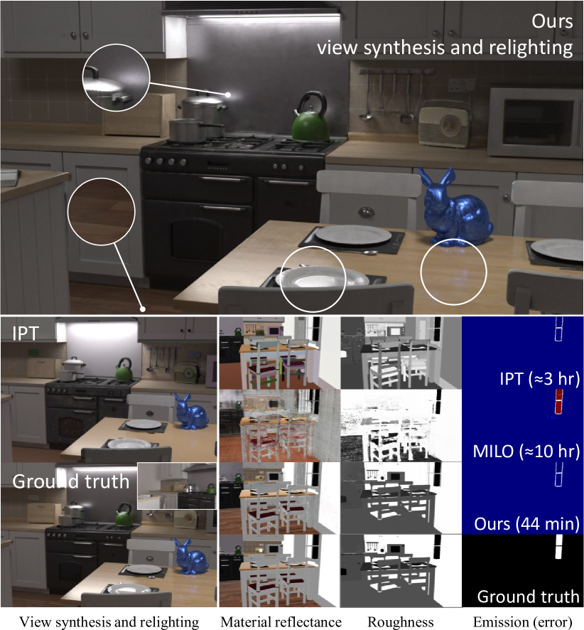
Figure 1: Ours vs standard IPT. IPT [1] takes a piecewise constant parameterization of material to reduce Monte Carlo variance and ambiguity for inverse rendering, losing fine spatial details as a result. Directly extending it to complex material representation (e.g. MILO [51]) shows very slow convergence. In contrast, we propose Factorized Inverse Path Tracing (FIPT) to get rid of variance and reduce ambiguities, yielding efficient and high quality BRDF and emission (4th row), appealing relighting (1st row), and object insertion (the bunny on the table). The presented scene is synthetic with the inset showing the input (lower-left sub-figure). We further showcase results on real scenes in Fig. 10 and  11.

Optimizing scene parameters with Monte Carlo differentiable rendering can suffer from high variance and lead to slow convergence. Inspired by classical irradiance caching literature [49], our key idea to address this challenge is to factorize the material term out of the rendering integral and bake the incoming radiance to significantly speed up inverse rendering. Unlike prior work which also applies a similar factorization (e.g. [37, 25]) but does not consider view-dependent reflections, our method extends to general specular materials and both local and global illumination.

To address the ill-posed nature of joint optimization of material and lighting, we observe that by taking out the emission term in the rendering equation for the first bounce, only emissive surfaces will have high rendering loss. This observation allows us to design an effective way to detect emitters. We incorporate our emitter detection method into a full inverse rendering pipeline and independently estimate the emission after emitter detection.

Overall, our method achieves fast convergence over the material-lighting estimation task thanks to our factorized light transport formulation and emitter extraction strategy (Fig. 1). To demonstrate accurate BRDF-emission comparison, we perform exhaustive experiments on synthetic scenes (Sec. 5.1, 5.2) while also validating on noisy data of captured real scenes (Sec. 5.3). The results show our method is able to obtain high-quality reconstruction for complicated indoor scenes that can easily fail for the state-of-the-art (Tab. 2), yet the training speed is 4-10 times faster (Tab. 3).

2 Related Work

Inverse rendering.

Inverse rendering aims to estimate the intrinsic properties of an observed scene, via decoupling material, geometry and lighting which jointly contribute to image appearance. Given the inherent ambiguity between the aforementioned high-dimensional factors, classical methods seek to regularize the solution with a surface rendering objective. Approaches include a low-dimensional surface reflectance representation [52], sparsity priors for intrinsic images [4], and spherical-harmonics-based lighting representation [29]. These methods rely on simplified representation of material or lighting, and their regression-based nature calls for heuristic-based priors which may not be appropriate for a wide variety of scenes.

Earlier work can already photorealistically render synthetic objects in a photograph by estimating lighting and geometry [12, 18, 19]. These methods do not retrieve the materials of the scene, and thus cannot show the reflection of the object on a specular surface in the scene.

Learning-based methods.

Learning-based approaches leverage priors learned from datasets. These methods typically take a single image [41, 23, 57, 48, 24] or a pair of stereo images [44], and apply deep learning models to predict spatially-varying materials and lighting. Although learned priors help to regularize individual components, these methods do not explicitly model the physics of global light transport and have to rely on approximated inference [27].

Philip et al. [37] take multiple images and aggregate multiview irradiance and albedo information to a pre-trained network to synthesize the relit image. The network takes physically rendered shading using light sources that are semi-automatically estimated as inputs, and outputs an image after relighting. We show in the results that in our synthetic scenes, their method’s reliance on the network to render the final image can lead to undesired artifacts, while our use of a physically-based renderer delivers more realistic images.

Local or distant lighting.

Many recent methods aim to model a specific form of light transport. Some methods focus on a single object or distant illumination (environment map) [14, 55, 32, 7, 8, 56]. Srinivasan et al. [43] model two-bounce volumetric lighting with known light sources, and Yao et al. [50] represent incident radiance as a 5D network. However, optimization of spatially-varying lighting without physically-based constraints is extremely ill-posed especially without abundant observation of light sources. Moreover, object-centric methods do not trivially generalize to indoor settings, where complex lighting effects including occlusion, inter-reflections, and directional highlights call for modeling of long-range interactions of lighting and scene properties.

Global light transport.

Most related to our work, to model general global light transport, recent methods [1, 33, 51] build on a per-scene optimization pipeline using a differentiable path tracer [22, 3, 34, 54]. These methods jointly optimize material and lighting along extensively sampled light paths, and thus are subject to incorrect and slow convergence and high variance due to expensive path queries, gradient propagation, and Monte Carlo sampling, as well as the inherent ambiguity between materials and lighting. We propose an inverse rendering pipeline that models the global light transport, but converges significantly faster and more accurately than existing methods. Our variance reduction technique using light baking is inspired by classical rendering methods [49, 21, 42], and we tightly integrate the technique in an inverse rendering pipeline. A concurrent work TexIR [26] adopts similar ideas to ours by using a pre-baked irradiance as HDR texture map to recover scene materials. However, they do not model view-dependent light transport and do not estimate emission.

3 Background

$(\cdot)_{+}$	dot product clamped to positive value
$\bm{\omega}_{i}$	incident (light) direction
$\bm{\omega}_{o}$	outgoing (viewing) direction
$\mathbf{h}$	half vector: $(\bm{\omega}_{i}+\bm{\omega}_{o})/\lVert\bm{\omega}_{i}+\bm{\omega}_{o}\lVert_{2}$
$\mathbf{n}$	surface normal
$\mathbf{a}(\mathbf{x})$	surface base color
$m(\mathbf{x})$	surface metallic
$\sigma(\mathbf{x})$	surface roughness
$\mathbf{k}_{d}(\mathbf{x})$	diffuse reflectance: $\mathbf{a}(\mathbf{x})(1-m(\mathbf{x}))$
$\mathbf{k}_{s}(\mathbf{x})$	specular reflectance: $\mathbf{a(\mathbf{x})}m(\mathbf{x})+0.04(1-m(\mathbf{x}))$
$D(\cdot)$	GGX normal distribution [47]
$F(\cdot)$	Schlick’s approximation of Fresnel coefficient [39]
$G(\cdot)$	Geometry (Shadow-Masking) term [47]

Table 1: Notations

Given posed HDR image captures of an indoor scene, our method builds upon input mesh or existing 3D reconstruction algorithms (e.g. MonoSDF [53]) to further estimate the material and lighting of the scene. To ensure the problem is well-constrained, we make similar assumptions about scene acquisition as in previous works [1, 37, 51] that the dominant light sources and most of the scene geometry are observed in input images.

The material is described as a spatially varying BRDF [17] (including the cosine term) with notations specified in Tab. 1:

$$\begin{gathered}f(\mathbf{x},\bm{\omega}_{i},\bm{\omega}_{o})=\frac{\mathbf{k}_{d}(\mathbf{x})}{\pi}\left(\mathbf{n}\cdot\bm{\omega}_{i}\right)_{+}\\ +\frac{F(\bm{\omega}_{i},\mathbf{h},\mathbf{k}_{s}(\mathbf{x}))D(\mathbf{h},\mathbf{n},\sigma(\mathbf{x}))G(\bm{\omega}_{i},\bm{\omega}_{o},\mathbf{n},\sigma(\mathbf{x}))}{4(\mathbf{n}\cdot\bm{\omega}_{o})},\end{gathered}$$ (3)

where $\mathbf{k}_{d}=\mathbf{a}(1-m)$ and $\mathbf{k}_{s}=0.04(1-m)+\mathbf{a}m$ are the diffuse and specular reflectance with base color $\mathbf{a}$ and metallic $m$ controlling the two coefficients. The emitted light is assumed to be view-independent across the surface: $\mathbf{L}_{e}(\mathbf{x},\bm{\omega}_{o})=\mathbf{L}_{e}(\mathbf{x})$, which generalizes well to the emission profile of the indoor scene (extension to more complex emitters is possible; see Sec. 5.4).

With the parameterization above, our goal is to find $\mathbf{a},\sigma,m,\mathbf{L}_{e}$ that minimize the difference of renderings with respect to the ground truth over the training images:

$$\min_{\mathbf{a},\sigma,m,\mathbf{L}_{e}}\sum_{\mathbf{x},\bm{\omega}_{o}}\left\|\mathbf{L}_{o}(\mathbf{x},\bm{\omega}_{o})-\mathbf{L}_{gt}(\mathbf{x},\bm{\omega}_{o})\right\|_{2}^{2}$$ (4)

$$\mathbf{L}_{o}(\mathbf{x},\bm{\omega}_{o})=\mathbf{L}_{e}(\mathbf{x},\bm{\omega}_{o})+\mathbf{L}_{r}(\mathbf{x},\bm{\omega}_{o})$$ (5)

$$\mathbf{L}_{r}(\mathbf{x},\bm{\omega}_{o})=\int_{\Omega^{+}}\mathbf{L}_{i}(\mathbf{x},\bm{\omega}_{i})f(\mathbf{x},\bm{\omega}_{i},\bm{\omega}_{o})d\bm{\omega}_{i}.$$ (6)

$\mathbf{L}_{gt}$ is a ground truth RGB pixel obtained from camera ray $(\mathbf{x},\bm{\omega}_{o})$. $\mathbf{L}_{o}$ denotes the synthesized rendering following the rendering equation [16], where $\mathbf{L}_{e}$ is the surface emitted radiance and $\mathbf{L}_{r}$ is the reflected radiance, given by integrating incident radiance $\mathbf{L}_{i}$ times the BRDF response (Eq. 6). Note, $\mathbf{L}_{i}$ is defined in a recursive manner with multi-bounce illumination naturally taken into account of.

4 Factorized Inverse Path Tracing

To optimize re-rendering error (Eq. 4), previous works [1, 33] apply differentiable path tracing to solve Eq. 5 and update BRDF and emission jointly with gradient descent. This approach can be unstable and inefficient: (1) gradient descent optimization is computationally intensive, which limits the number of path tracing samples and therefore increases the estimation variance; (2) fundamental ambiguities exist between BRDF and emission, making emission optimization difficult to regularize or converge. To reduce variance in optimization, we propose a factorized light transport representation (Sec. 4.1) which utilizes pre-baking of diffuse and specular shading maps (Eq. 8) to separate the BRDF coefficients out of the rendering integral.

Our full pipeline is demonstrated in Fig. 2, which optimizes dense BRDF and emission from posed images and scene geometry. The pipeline consists of 3 stages: (1) first, the factorized diffuse and specular shadings are initialized (baked) as described in Sec. 4.2; (2) given baked shadings, BRDF and emission mask are then optimized (Sec. 4.5), followed by emitter extraction (Sec. 4.4); (3) given current BRDF-emission estimation, the shadings are refined (Sec. 4.3), and the algorithm alternates between (2) and (3) until convergence.

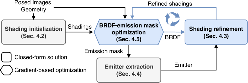
Figure 2: Our inverse rendering pipeline approximates diffuse and specular shadings from input images and geometry, which are used for efficient renderings during the BRDF-emitter optimization. The optimized BRDF and emitters are then passed into a path tracer to refine shadings. The BRDF and the shadings are then updated alternatively.

4.1 Factorized light transport

A common way to speed up path tracing in the rendering literature [49, 21, 42] is to factor the BRDF from the rendering integral, and then to pre-bake and reuse the integral parts. Employing a similar idea, we rewrite the reflection equation (Eq. 6) as:

$$\begin{split}\mathbf{L}_{r}(\mathbf{x},\bm{\omega}_{o})&=\mathbf{k}_{d}\mathbf{L}_{d}(\mathbf{x})\\ &+\mathbf{k}_{s}\mathbf{L}_{s}^{0}(\mathbf{x},\bm{\omega}_{o},\sigma)+\mathbf{L}_{s}^{1}(\mathbf{x},\bm{\omega}_{o},\sigma)\end{split}$$ (7)

$$\begin{split}\mathbf{L}_{d}(\mathbf{x})&=\int_{\Omega^{+}}\mathbf{L}_{i}(\mathbf{x},\bm{\omega}_{i})\frac{(\mathbf{n}\cdot\bm{\omega}_{i})_{+}}{\pi}d\bm{\omega}_{i}\\ \mathbf{L}_{s}^{0}(\mathbf{x},\bm{\omega}_{o},\sigma)&=\int_{\Omega^{+}}\mathbf{L}_{i}(\mathbf{x},\bm{\omega}_{i})\frac{F_{0}DG}{4(\mathbf{n}\cdot\bm{\omega}_{o})}d\bm{\omega}_{i}\\ \mathbf{L}_{s}^{1}(\mathbf{x},\bm{\omega}_{o},\sigma)&=\int_{\Omega^{+}}\mathbf{L}_{i}(\mathbf{x},\bm{\omega}_{i})\frac{F_{1}DG}{4(\mathbf{n}\cdot\bm{\omega}_{o})}d\bm{\omega}_{i},\end{split}$$ (8)

where $\mathbf{L}_{d}$ is the diffuse shading; $\mathbf{L}_{s}^{0},\mathbf{L}_{s}^{1}$ are the two specular shadings associated with two Fresnel components [39]:

$$\begin{gathered}F(\mathbf{h},\bm{\omega}_{i},\mathbf{k}_{s}(\mathbf{x}))=\mathbf{k}_{s}(\mathbf{x})F_{0}+F_{1}\\ F_{0}=\left(1-(1-\mathbf{h}\cdot\bm{\omega}_{i})^{5}\right),F_{1}=(1-\mathbf{h}\cdot\bm{\omega}_{i})^{5}.\end{gathered}$$ (9)

The specular shadings are further approximated by linear interpolation of 6 pre-defined roughness levels:

$$\mathbf{L}_{s}^{*}(\cdot,\sigma)\approx\text{lerp}(\{\mathbf{L}_{s}^{*}(\cdot,\sigma_{k})|\sigma_{k}\in\text{linspace(0,1,6)}\},\sigma),$$ (10)

such that $\mathbf{k}_{d},\mathbf{k}_{s},\sigma$ are all separated out of the integral.

With this factorization, we can bake the shadings $\mathbf{L}_{d},\mathbf{L}_{s}^{0},\mathbf{L}_{s}^{1}$ offline for each input view into image buffers, then query the shading pixels at training time to speed up rendering. Baking shadings offline allows us to use a large sampling rate for variance reduction. Owing to its linear formulation, we also empirically found this factorized rendering handles mirror-like objects much better (Fig. 9), while standard Monte Carlo integration can easily obtain unstable gradients caused by the large BRDF value.

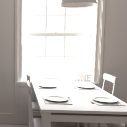
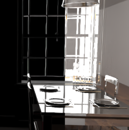
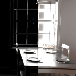
	Estimated
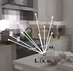
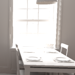
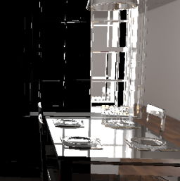
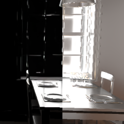
	Ground truth $\mathbf{L}_{d}$ $\mathbf{L}_{s}^{*}(\sigma=0.02)$ $\mathbf{L}_{s}^{*}(\sigma=0.2)$

Figure 3: Diffuse and specular shadings are initialized by tracing a voxel representation of the surface light field $\mathbf{L}^{\prime}$ (left), which gives approximations (top row on right) close to the ground truth (bottom row on the right; obtained by path tracing).

4.2 Image-based shading initialization

As we pre-bake the shadings $\mathbf{L}_{d},\mathbf{L}_{s}^{0},\mathbf{L}_{s}^{1}$, they are fixed during BRDF-lighting estimation. They need to be properly initialized; otherwise, the optimization will not converge. For simplicity, we abstract the integrands in Eq. 8 to the form: $\mathbf{L}_{*}=\mathbf{L}_{i}g$, where $g$ denotes the factorized BRDF term. In path tracing notation, the shading integral can be initialized by querying a surface light field approximation:

$$\begin{gathered}\mathbf{L}_{*}(\mathbf{x})=\mathbf{L}(\mathbf{x}_{1}\rightarrow\mathbf{x})g(\mathbf{x}_{1}\rightarrow\mathbf{x})\\ \approx\mathbf{L}^{\prime}(\mathbf{x}_{1})g(\mathbf{x}_{1}\rightarrow\mathbf{x}),\end{gathered}$$ (11)

where $\mathbf{L}$ is the exact surface light field at sampled location $\mathbf{x}_{1}$ towards $\mathbf{x}$, and $\mathbf{L}^{\prime}$ is its approximation obtained by average pooling all the input pixels onto a voxel grid spanned on the scene geometry (Fig. 3 left). Since objects in an indoor scene are often near-diffuse, and the renderings are essentially low pass filtering the incident light field [38] that blurs the detail, we find that using a $256^{3}$ voxel grid with nearest neighbor radiance query gives good shading approximations (Fig. 3 right).

4.3 Path-traced shading refinement

Eq. 11 gives incorrect shading if the surface light field is sampled at locations that are mainly specular ($\mathbf{L}$ is view dependent), which subsequently leads to incorrect BRDF estimation. Given BRDF-emitter estimations optimized from Eq. 4 under current shading estimations, we re-estimate the light transport on specular surfaces by growing the path in Eq. 11 until the ray either hits an emitter or intersects with a near diffuse surface (identified by $\sigma>0.6$; Fig. 4):

$$\begin{gathered}\mathbf{L}_{*}(\mathbf{x})=\mathbf{R}(\mathbf{x}_{n})\prod_{i=1}^{n-1}f(\mathbf{x}_{i+1}\rightarrow\mathbf{x}_{i})g(\mathbf{x}_{1}\rightarrow\mathbf{x}),\\ \text{s.t. }\sigma(\mathbf{x}_{i})\leq 0.6\text{, }\forall i<n\end{gathered}$$ (14)

$$\mathbf{R}(\mathbf{x}_{n})=\begin{cases}\mathbf{L}^{\prime}(\mathbf{x}_{n})&\sigma(\mathbf{x}_{n})>0.6\\ \mathbf{L}_{e}(\mathbf{x}_{n})&\mathbf{L}_{e}(\mathbf{x}_{n})>0\end{cases},$$ (15)

where $n$ is the length of a certain path before it terminates. The above equation essentially estimates the shadings by multi-bounced path tracing with $\mathbf{L}^{\prime}$ being a diffuse radiance cache, which helps speed up the evaluation and also reduce error: initial estimations of $f$s may retain large error but $\mathbf{L}^{\prime}$ is very close to a diffuse surface light field (as it is also view-independent). Most of the path hits a diffuse surface within one to two bounces, such that the errors from the BRDF will not be magnified (Fig. 5).

Substituting shadings in factorized rendering by their refinements makes Eq. 7 more closely match the ground truth light transport, such that BRDF can be re-estimated with fewer artifacts (Fig. 4: ‘Origin’ VS ‘Refined’). The re-estimated BRDF in turn is applied to further improve the shadings, and this BRDF and shading refinement is performed alternatively until convergence.

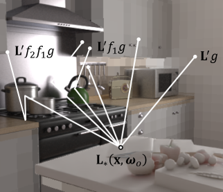
Origin Refined Ground truth

Figure 4: Shading refinement: The cabinet’s diffuse reflectance estimation is initially darker than ground truth, owing to the excessive incident light received from the range hood that reflects non-diffuse light (2nd column). The artifacts are reduced by growing the path for the specular surface according to the optimized BRDF (1st column), which gives more accurate shadings that can be used to further refine the BRDF (3rd column).

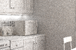
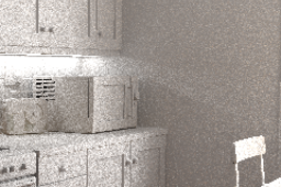
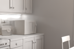
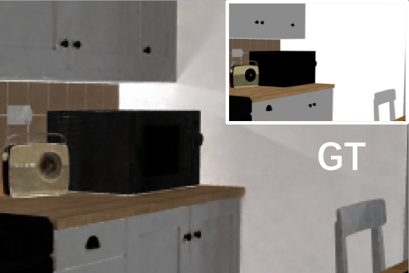
w/o cache	w/ cache	GT	$\mathbf{k}_{d}$ w/o cache

Figure 5: Diffuse radiance cache from $\mathbf{L}^{\prime}$ helps reduce variance and error for shading estimation (2nd image). Without it, sampling the tiny emitters below the cabinet will be difficult (1st image), which leads to incorrect shading and albedo (4th image).

4.4 Error-driven emitter estimation

If we replace rendering equation Eq. 5 by Eq. 6 that excludes the emission, the objective Eq. 4 still converges for non-emissive surfaces (as their $\mathbf{L}_{e}=0$), but regions with emission will present large errors, which is a good indicator of emitters (Fig. 6). With this intuition, we introduce an emission mask (encouraged to be small) $\alpha\in[0,1]$ to the rendering loss:

$$\begin{gathered}\min_{\mathbf{a},\sigma,m,\alpha}\sum_{\mathbf{x},\bm{\omega}_{o}}\left\|(1-\alpha)\mathbf{L}_{r}+\alpha\mathbf{L}_{gt}-\mathbf{L}_{gt}\right\|_{2}^{2}\\ \text{s.t. }\alpha\rightarrow 0.\end{gathered}$$ (18)

When a surface is non-emissive, $\alpha$ will stay small owing to the regularization and the loss is minimized by adjusting $\mathbf{L}_{r}$ towards $\mathbf{L}_{gt}$; but $\mathbf{L}_{r}$ cannot model the emission, so $\alpha$ for an emissive surface has to become large to accommodate the error. In practice we apply a L1 sparsity loss to $\alpha$. By changing the optimization objective to Eq. 18, we first jointly estimate the BRDF-emission mask, and then threshold the mask to find the emitter ($\alpha>0.01$). Afterward, each emitter’s emission $\mathbf{L}_{e}$ is estimated independently from BRDF:

$$\mathbf{L}_{e}=\begin{cases}\underset{\mathbf{L}_{e}}{\arg\min}\underset{\mathbf{x},\bm{\omega}_{o}}{\sum}\left\|\mathbf{L}_{e}+\mathbf{L}_{r}-\mathbf{L}_{gt}\right\|_{1}&\alpha>0.01\\ 0&\text{otherwise}\end{cases}.$$ (19)

Our formulation is found to be more stable than joint optimization (demonstrated in ablations in Sec. 5.4), because the emission mask value is in the same range as BRDF coefficients, such that the gradient update is balanced between the BRDF and the emission mask. In contrast, surface emission can be much larger than BRDF coefficients, making it more difficult to directly fit or regularize.

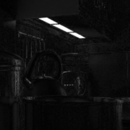
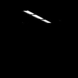
RGB	GT emission	Rendering error	Emission mask

Figure 6: Rendering images without emission terms produces distinctive error near emissive surfaces (3rd image). By jointly optimizing an emission mask (4th image) to cancel this error, the emitter can be found by checking the mask’s response, which is robust even for tiny emitters (2nd image for ground truth).

Emitter extraction.

We assume emission is constant for each mesh triangle. After $\alpha$ is optimized, we uniformly sample 100 locations on each triangle and find their corresponding $\alpha$ value. A triangle is then classified as an emitter if the mean of its $\alpha$s is above 0.01. Eq. 19 in general is ill-posed (e.g. $\mathbf{k}_{d}$ can be increased by decreasing $\mathbf{L}_{e}$), so we make the assumption that an emitter reflects zero light ($f=0$). In such a situation, $\mathbf{L}_{e}$ for a triangle has the closed-form solution as the median of RGBs from all input pixels it intersects, which does not require any gradient descent optimization, so it can be estimated efficiently and accurately.

4.5 Optimization

Given either initial or refined shadings, the BRDF and emission mask are optimized using the objective in Eq. 18. We encode BRDF and the emission mask with two MLPs:

$$\begin{gathered}(\mathbf{a},m,\sigma)=\text{Sigmoid}\left(\text{MLP}_{\text{brdf}}(\mathbf{x})\right)\\ \alpha=1-\exp{\left(-\text{ReLU}(\text{MLP}_{\text{emit}}(\mathbf{x}))\right),}\end{gathered}$$ (20)

where $\text{MLP}_{\text{brdf}}$ uses hash encoding [31] and $\text{MLP}_{\text{emit}}$ is a positional encoded MLP [30]. The objective Eq. 18 is converted to a gradient descent loss function as a tone-mapped L2 loss $l$ plus a L1 regularization term $l_{e}$:

$$l=\sum_{\mathbf{x,o}}\left\|\Gamma((1-\alpha)\mathbf{L}_{r}+\alpha\mathbf{L}_{gt})-\Gamma(\mathbf{L}_{gt})\right\|_{2}^{2}$$ (21)

$$l_{e}=\lambda_{e}\sum_{\mathbf{x}}\|\text{MLP}_{\text{emit}}(\mathbf{x})\|_{1},\lambda_{e}=1,$$ (22)

where $\Gamma$ is the tone-mapping function by Munkberg et al. [32] to help suppress noise from high dynamic range values. We prefer neural networks rather than a textured mesh (as in [1, 33]) as scenes with complex geometries can create degenerate UVs, which reduces the BRDF quality.

Roughness-metallic regularization.

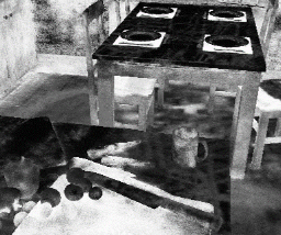
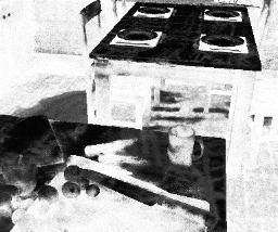
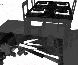
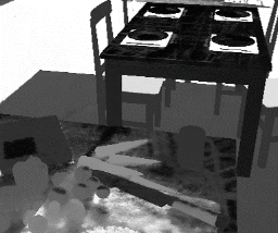
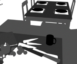
w/o $l_{d},l_{p}$	w/o $l_{p}$	w/ part	w/ semantic	GT

Figure 7: Roughness optimization can be ambiguous without any regularization (1st image). By encouraging a surface to be diffuse, specular surfaces still get an incorrect roughness value if no highlights are observed (2nd image). The roughness can be more reasonably estimated with part segmentation for guidance (3rd image). Semantic segmentation (4th image) shows similar results except the roughness for small objects get blurred.

Surface roughness and metallic can take arbitrary values if there are no highlights ($\mathbf{L}_{s}^{0},\mathbf{L}_{s}^{1}\approx 0$), which leads to ambiguity. We prevent this by encouraging surfaces to be diffuse:

$$l_{d}=\lambda_{d}\sum_{\mathbf{x}}\left(\|1-\sigma(\mathbf{x})\|_{1}+\|m(\mathbf{x})\|_{1}\right),\lambda_{d}=\text{5e-4},$$ (23)

such that a diffuse surface will not be misinterpreted as a specular surface with weak reflection. To get valid roughness-metallic for input pixels that do not observe highlights, we further assume they stay constant inside each material part, and utilize image-level part segmentation to group input pixels. The roughness-metallic from pixels with highlights are propagated to their corresponding group by another regularization loss:

$$l_{p}=\lambda_{p}\sum_{\mathbf{x}}\left\|\begin{bmatrix}\sigma(\mathbf{x})\\ m(\mathbf{x})\end{bmatrix}-\begin{bmatrix}\sigma^{\prime}(\mathbf{x})\\ m^{\prime}(\mathbf{x})\end{bmatrix}\right\|_{1},\lambda_{p}=\text{5e-3}$$ (24)

$$\begin{gathered}\begin{bmatrix}\sigma^{\prime}(\mathbf{x})\\ m^{\prime}(\mathbf{x})\end{bmatrix}=\sum_{\text{Seg}(\mathbf{x^{\prime}})=\text{Seg}(\mathbf{x})}\frac{w(\mathbf{x^{\prime}})}{\sum_{\mathbf{x}^{\prime}}w(\mathbf{x}^{\prime})}\begin{bmatrix}\sigma(\mathbf{x^{\prime}})\\ m(\mathbf{x^{\prime}})\end{bmatrix}\\ w(\mathbf{x^{\prime}})=\text{sg}\left(\|\mathbf{k_{s}}\mathbf{L}_{s}^{0}+\mathbf{L}_{s}^{1}\|_{1}\right),\end{gathered}$$ (27)

where $\text{Seg}(\mathbf{x})$ gives the segmentation ID for $\mathbf{x}$, $\text{sg}(\cdot)$ denotes stop the gradient, and $w(\mathbf{x})$ is a propagation kernel that weights the pixel by the amount of highlights. While part segmentation in practice can be hard to obtain, semantic segmentation is readily available from pre-trained model e.g. Mask2Former [11], where multiple material parts may stay inside the same semantic label. To account for such detail loss, we consider two pixels belong to the same material part only if: (1) they share the same semantic ID; (2) have similar albedo value; (3) and are close to each other, which suggests an alternative propagation kernel $w(\mathbf{x,x^{\prime}})$:

$$\begin{gathered}w(\mathbf{x}^{\prime},\mathbf{x})=\text{sg}\left(e^{-\frac{\|\mathbf{a}(\mathbf{x})-\mathbf{a}(\mathbf{x^{\prime}})\|_{2}^{2}}{2\sigma_{a}^{2}}}e^{-\frac{\|\mathbf{x}-\mathbf{x^{\prime}}\|_{2}^{2}}{2\sigma_{x}^{2}}}\right)\\ \sigma_{a}=\text{1.6e-2},\sigma_{x}=\text{1e-2}.\end{gathered}$$ (28)

By replacing $\mathbf{w}(\mathbf{x})$ with $\mathbf{w}(\mathbf{x,x}^{\prime})$ and changing the regularization weight to $\lambda_{p}=\text{1e-3}$, we can still have reasonable roughness-metallic estimation even with semantic segmentation (Fig. 7).

5 Experiments

BRDF and emission estimation
Li22 [24]	IPT [1]	FIPT	Ground truth	Li22 [24]	IPT [1]	FIPT	Ground truth

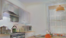
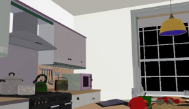
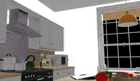
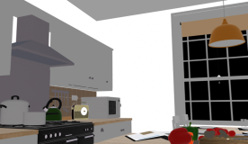
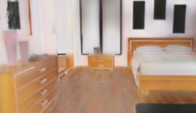
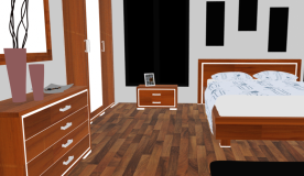
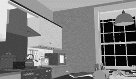
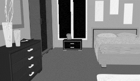
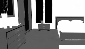
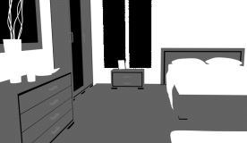
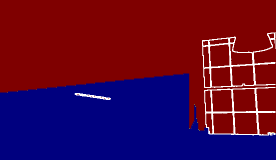
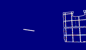
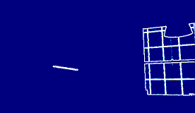
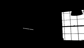
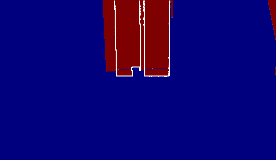
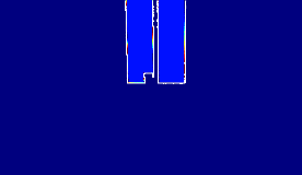
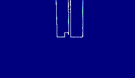
Figure 8: BRDF and emission estimation results on 2 synthetic scenes shows our method successfully reconstructs material reflectance (1st row), roughness (2nd row), and emission (3rd row) with high frequency details and less ambiguity. Emission estimation is shown as error heatmaps (warmer colors indicate higher emission error; GT emitter boundary is marked in white lines). Input views are shown in upper-right corner.

View synthesis				Relighting
FVP [37]	IPT [1]	FIPT	Ground truth	FVP [37]	IPT [1]	FIPT	Ground truth

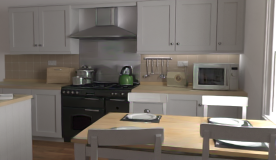
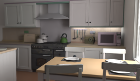
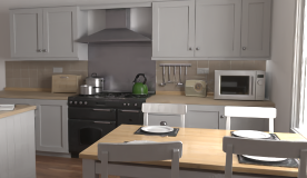
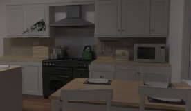
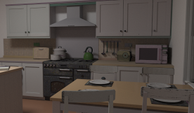
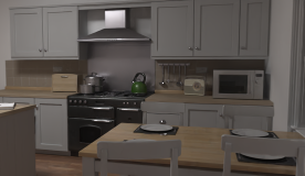
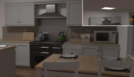
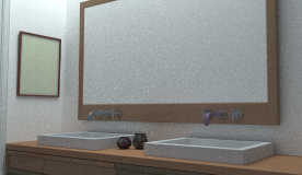
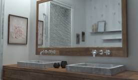
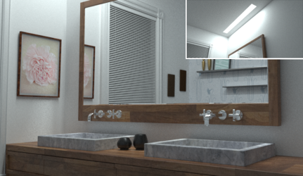
Figure 9: Qualitative results of view synthesis (left) and relighting (right) on 2 synthetic scenes demonstrate accurate light transport can be simulated with our estimated BRDF and emission even for very specular surfaces. The reflection of the chair from the microwave oven can be seen in kitchen scene on top, and mirrors are correctly rendered for bathroom (bottom).

We evaluate our method on 4 synthetic and 2 real indoor scenes, where the synthetic scenes are obtained from Bitterli’s rendering resources [5] with large glass objects being removed (as we do not model transmission), and the real scenes are captured by us. Each synthetic scene contains around 200 posed HDR images generated by Mitsuba3 [15], per-camera view BRDF-emission maps generated by Blender [6], and ground truth geometry. For synthetic scenes, we show our method with both part segmentation (FIPT) and semantic segmentation mask (FIPT-sem).

The real scenes (Conference room and Classroom) are captured by a Sony A7M3 camera with around 200 HDR images reconstructed by 5-stop exposure bracketing. The camera poses are estimated from COLMAP [40] and the geometry is reconstructed using MonoSDF [53]. Please refer to the supplementary material for details on real scene capturing and additional results.

5.1 Synthetic: BRDF-emission estimation

While synthetic scenes allow us to directly compare with the ground truth BRDF-emission without noise from geometry or image captures, BRDF parameterizations can vary across different baselines. For fair comparison, we empirically found diffuse reflectance $\mathbf{k}_{d}$ for diffuse surfaces, roughness $\sigma$, and the material reflectance defined by $\mathbf{a}^{\prime}=\int_{\Omega^{+}}fd\bm{\omega}_{i}$ are very close across different BRDF models [9, 17]. We therefore measure the PSNR for these metrics in image space for BRDF comparison. The $\mathbf{k}_{d}$ is compared only for diffuse surfaces, and $\mathbf{a}^{\prime}$ is estimated using Monte Carlo integration of 128 samples per pixel. For emission, we estimate the IoU of emission mask and $\log\text{L2}$ error of emission map.

Baselines.

We compare with the original inverse path tracing (IPT) [1] and its extension MILO [51] that also parameterizes spatially varying BRDF with neural networks. IPT assumes BRDF parameters to be constant inside each mesh triangle, and MILO takes manual input of number of emitters. Both IPT and MILO are evaluated by their original authors due to non-public code, and the MILO training is stopped after 10 hours. Meanwhile, we also compare NeILF [50] that models illumination in an unconstrained way and the learning based approach [24] (Li22) for single-view inverse rendering.

	Method	$\mathbf{k}_{d}$	$\mathbf{a}^{\prime}$	$\sigma$	$\mathbf{L}_{e}$
		PSNR$\uparrow$			IoU$\uparrow$	logL2$\downarrow$
Bathroom	Li22 [24]	19.92	15.78	13.77	0.45	1.35
	NeILF [50]	10.12	9.01	14.82	-	-
	IPT [1]	22.43	18.59	14.69	0.33	1.09e-1
	MILO [51]	11.83	9.80	5.56	0.05	5.60e-1
	FIPT	30.13	25.28	28.79	0.63	3.18e-2
	FIPT-sem	27.81	24.00	21.84	0.63	3.18e-2
Bedroom	Li22 [24]	21.87	17.18	12.12	0.34	2.78
	NeILF [50]	14.88	12.42	11.30	-	-
	IPT [1]	29.39	22.46	13.33	0.92	4.01e-3
	MILO [51]	23.65	15.16	15.42	0.08	1.59e-2
	FIPT	31.10	29.41	23.19	0.96	4.95e-4
	FIPT-sem	31.00	28.45	25.23	0.96	4.93e-4
Livingroom	Li22 [24]	17.25	15.32	12.72	0.17	3.61
	NeILF [50]	12.34	10.97	13.45	-	-
	IPT [1]	21.24	19.01	11.77	0.90	6.08e-3
	MILO [51]	22.88	18.39	13.98	0.06	1.39e-2
	FIPT	28.86	28.70	32.48	0.95	8.06e-4
	FIPT-sem	29.09	28.62	25.15	0.95	8.09e-4
Kitchen	Li22 [24]	18.14	14.54	10.82	0.43	1.41
	NeILF [50]	12.63	9.96	10.64	-	-
	IPT [1]	25.68	21.61	11.84	0.83	1.08e-2
	MILO [51]	18.25	13.86	12.56	0.10	8.28e-2
	FIPT	33.07	27.53	29.24	0.91	1.54e-3
	FIPT-sem	33.25	27.38	21.70	0.91	1.54e-3

Table 2: BRDF-emission comparison on synthetic scenes shows that our method gives the overall best reconstruction. The results are similar even if only semantic segmentation is provided (FIPT-sem). NeILF does not estimate emitters. The best method is marked in bold.

Our per-stage profiling Stage 1 Stage 2 Stage 3 Memory 3.2GB 2.8GB 3.4GB Time 6min 2min 16min

Method training time$\downarrow$ NeILF [50] 1h38min IPT [1] $\approx$3hr MILO [51] $\approx$10hr FIPT 44min

Table 3: Averaged training speed comparison suggests our method is very efficient (right table). The per-stage profiling is shown on the left with Stage 2 and 3 being repeated twice. The comparison is made on a 3090Ti GPU.

Results.

As is shown in Tab. 2, our method gives the best BRDF and emission estimation with the fastest training speed (Tab. 3) even when only semantic level segmentation is provided (FIPT-sem). The learning-based approach (Li22) fails to generate reasonable reconstruction as it does not utilize multi-view cues, while unconstrained optimization (NeILF) suffers from the ambiguity between material and lighting. While IPT converges, its accuracy is limited by a piece-wise constant constraint to reduce the variance. MILO also fails to reconstruct high frequency details because of the Monte Carlo noise from path tracing, and it requires manual specification of the number of emitters to constrain the emission optimization. In contrast, our method requires no human input during optimization, which allows more stable and faster convergence with results that match the ground truth well (Fig. 8).

5.2 Synthetic: view synthesis and relighting

To demonstrate the applications of inverse rendering outputs, we compare the rendered scenes under novel views and novel lighting using estimated BRDF and emission. For quantitative comparison, we tone-map the rendered images with $\gamma=1/2.2$ then calculate their PSNR with respect to the ground truth.

Baselines.

Besides IPT, MILO, and Li22, we also consider FVP [37] that performs view synthesis and relighting in a learning-based way. FVP assumes emissions come from saturated regions on the images, which may wrongly classify surfaces with strong reflection as emitters. So we offer ground truth emission to FVP instead as oracle. The renderings for IPT, MILO, and our method are obtained by path tracing with 1024 samples per pixel, which is further denoised by the Optix denoiser [35].

	Method	Bathroom	Bedroom	Livingroom	Kitchen
View synthesis	FVP [37]	23.38	20.49	24.63	20.77
	IPT [1]	14.76	21.85	23.87	19.94
	MILO [51]	20.62	20.25	24.47	18.09
	FIPT	25.42	29.84	30.86	25.38
	FIPT-sem	25.76	29.89	30.84	25.27
Relight	Li22 [24]	22.86	23.20	19.83	21.76
	FVP [37]	23.72	24.11	19.51	23.31
	IPT [1]	20.61	28.16	27.26	27.28
	MILO [51]	14.97	23.39	22.10	19.62
	FIPT	31.28	36.64	31.56	29.13
	FIPT-sem	31.03	36.69	30.82	28.79

Table 4: Quantitative results (PSNR) of view synthesis and relighting on synthetic scenes show our estimation yields very consistent rendering under novel views and lighting. View synthesis is unavailable for Li22.

MILO [51]	Li22 [24]	FIPT	MILO [51]	Li22 [24]	FIPT	Input views

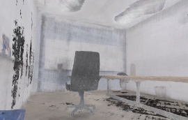
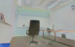
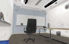
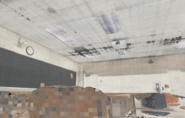
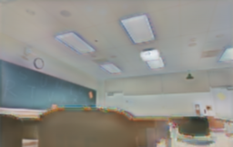
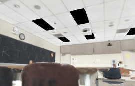
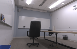
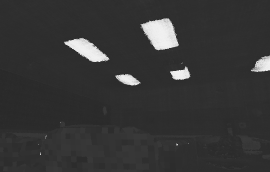
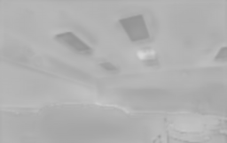
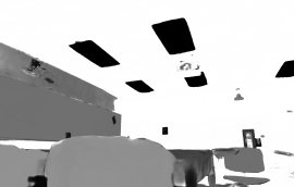
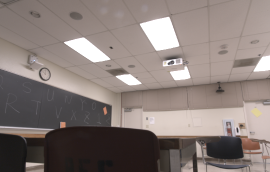
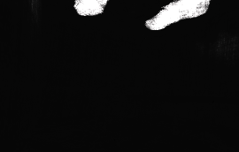
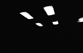
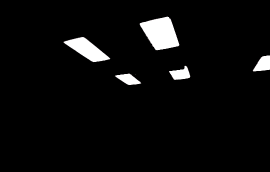
Figure 10: BRDF and emission estimation results on 2 real world scenes demonstrate our method gives reasonable estimation of BRDF and emission. The albedo and roughness preserve details without noticeable artifacts (row 1-2), and the emitters are correctly identified (3rd row).

Rerendering					Relighting
MILO [51]	Li22 [24]	FVP [37]	FIPT	Ground truth	MILO [51]	Li22 [24]	FVP [37]	FIPT

Figure 11: Rerendering and relighting on 2 real world scenes show our estimation fits the ground truth well (column 1-5) and gives good rendering under novel light (column 6-9). The inset in lower-right sub-figure shows the reference relighting for the Classroom scene.

Results.

As is shown in Tab. 4, our (FIPT and FIPT-sem) estimated BRDF-emission gives the most accurate view synthesis and relighting results. While results from FVP are seemingly visually appealing, the method is not guaranteed to be physically plausible and fails to match the ground truth. As shown in Fig. 9, our method handles specular reflections and even mirror reflection well, which is difficult to be modeled by standard inverse path tracing owing to its high variance.

5.3 Real-world scenes

Considering that it is not possible to obtain ground truth BRDF and emission from just RGB captures, we only showcase qualitative comparison with MILO, FVP, and Li22 in terms of material-lighting estimation, rerendering, and relighting. Only semantic segmentation is used for the real scenes as ground truth part segmentation is unavailable.

Results.

As is shown in Fig. 10, our method visually produces more reasonable material reflectance and roughness with emission masks closer to the actual emitters. The rerendering and relighting in Fig. 11 further serve as indirect measurements of the reconstruction quality, where our method is capable of reconstructing the reflection of the emitters on the Conference room wall and the Classroom table, and our relighting is visually closer to reference photos (obtained by switching lights; see supplementary) than the baselines with good reproduction of specular highlights and shadows.

5.4 Ablation study

Training strategy.

Tab. 5 shows the effect of different training strategies on the kitchen scene. If we jointly optimize the emission and BRDF with the regularization term in IPT [1], the BRDF optimization can still converge, but the emission estimation does not converge given the same amount of time (2 epochs). Since the majority of the scene receives incident light from nearby diffuse surfaces, the reconstruction result is still reasonable without shading refinement (stage 3), but further refining the BRDF estimation helps to correct light transport for specular surfaces. If we simply path-trace the BRDF-emission without using the radiance cache from stage 1, the refined shadings will accumulate too much estimation error causing the subsequent BRDF estimation to deviate from ground truth.

Training strategy	$\mathbf{k}_{d}$	$\mathbf{a}^{\prime}$	$\sigma$	$\mathbf{L}_{e}$
	PSNR$\uparrow$			IoU$\uparrow$	logL2$\downarrow$
Joint $\mathbf{L}_{e}$ opt.	32.31	25.50	22.77	0.10	6.62e-1
w/o stage 3	32.20	25.18	23.37	0.91	1.54e-3
w/o rad. cache	19.35	16.82	25.65	0.91	1.54e-3
Full model	33.07	27.53	29.24	0.91	1.54e-3

Table 5: Ablation study on training strategy shows joint BRDF-emission optimization can lead to slow convergence of the emission, and shading refinement helps further improve the reconstruction quality.

Segmentation artifacts		Geometry artifacts

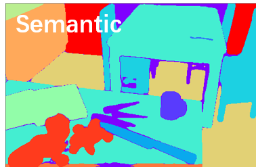
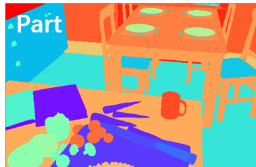
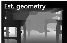
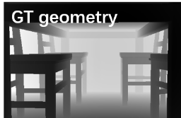
Figure 12: Example of input noise introduced by semantic segmentation and estimated geometry.

Training input	$\mathbf{k}_{d}$	$\mathbf{a}^{\prime}$	$\sigma$	$\mathbf{L}_{e}$		Relight
	PSNR$\uparrow$			IoU$\uparrow$	logL2$\downarrow$	PSNR$\downarrow$
Fewer views	32.64	26.7	28.80	0.91	1.57e-3	28.90
Est. geometry	27.01	22.57	21.33	0.78	0.1142	27.90
Semantic seg.	33.25	27.38	21.70	0.91	1.54e-3	28.79
Part seg.	33.07	27.53	29.24	0.91	1.54e-3	29.13

Table 6: Ablation study on training input shows our method gives similar performance with fewer training images. If the input geometry or the segmentation is not perfect (semantic segmentation), the reconstruction quality downgrades but can still give reasonable relighting.

Sensitive analysis on training inputs.

We run our algorithm on the kitchen scene with different setups: (1) using 60 training views instead of 200; (2) using geometry from MonoSDF [53] instead of the ground truth; (3) and replacing part segmentation by semantic segmentation. As is shown in Tab. 6, training with fewer views shows almost equal quality as long as they cover most of the scene. However, it still requires around 200 images in capturing to get good geometry reconstruction. Both estimated geometry and semantic segmentation introduce inaccuracy for detailed objects (Fig. 12), which disrupts roughness estimation for regions that see weak highlights. However, given the lighting for those regions is mostly ambiguous, it does not affect the overall reconstruction quality or relighting too much.

Complex geometry	Environment light

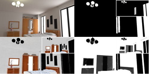
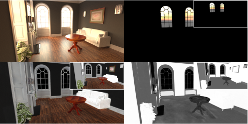
Figure 13: Reconstruction with complex emitters. Our method can also correctly identify complex lamps (first 2 columns) or environment lighting (last 2 columns) with reasonable BRDF reconstruction. Ground truth is shown in the insets.

Complex emitters.

Our method also works with lamp-like emitters with complex geometry (Fig. 13). For windows with hollow geometry, we can model the window light as a directional light source and let rays that fail to hit any indoor geometry to query an outdoor environment map. Each pixel of the environment map is estimated similarly as the emission of an emitter triangle. While environment lighting may not be fully observed and consequently causes artifacts near windows (see Sec. 6), a majority of the surfaces can still be reconstructed well owing to the diffuse radiance cache.

6 Limitations and Future Work

Bad input geometry		Insufficient emission observation

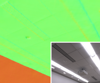
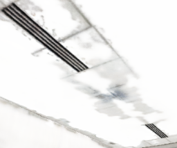
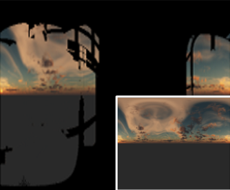
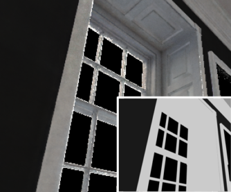
Figure 14: Limitations. Bad geometry estimation of an emitter (1st image) will lead to incorrect BRDF reconstruction of its nearby regions (2nd image). Incomplete observation of the environment light (3rd image) can cause artifacts in BRDF estimation (4th image).

Our method shares certain limitations with standard inverse path tracing. The framework does not optimize geometry, so that the BRDF and emission estimations can be inaccurate if the input geometry (especially for emitters) is extremely bad (Fig 14, left). Combining differentiable geometry optimization [2, 46] may help improve the robustness. Meanwhile, the BRDF estimation fails if the dominant light source (e.g. the sun) is not directly observed, which can happen very often with environment emitters whose observations are blocked by the windows (Fig. 14, right). Incorporating learning based methods may help. Lastly, the optimization relies on photometric observations, which means it cannot remove ambient occlusion effects out of the BRDF maps (as radiance there is near zero) and our model does not model transparent objects.

Acknowledgements.

This work was supported in part by NSF grants 1751365, 2100237, 2105806, 2110409, 2120019, 2127544, ONR grant N000142012529, N000142312526, a Sony research Award, gifts from Qualcomm, Adobe and Google, the Ronald L. Graham Chair and the UC San Diego Center for Visual Computing.

Additionally, we would like to thank Bohan Yu, Dejan Azinovic, Julien Philip, and Zhengqin Li for generous assistance in evaluation of their methods, David Forsyth, Shenlong Wang, and Merlin Nimier-David for insightful discussions, as well as Jiaer Zhang for assistance in implementation.

Supplementary Material Overview

In Sec. A, we provide the details of our pipeline implementation and data pre-processing.

In Sec. B, we present additional details of our experiments, including: (1) the setup of real world scenes (Sec. B.1); (2) detailed ablation study (Sec. B.2); (2) additional results (Sec. B.3); and (4) the schemes for evaluating the baselines (Sec. B.4).

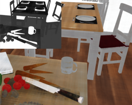
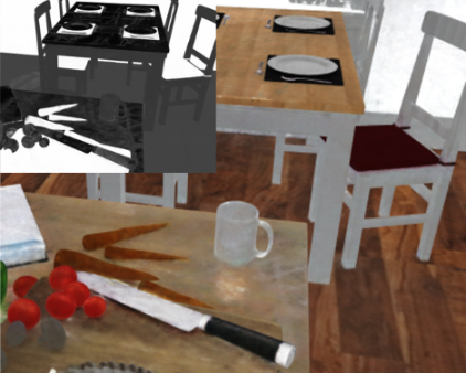
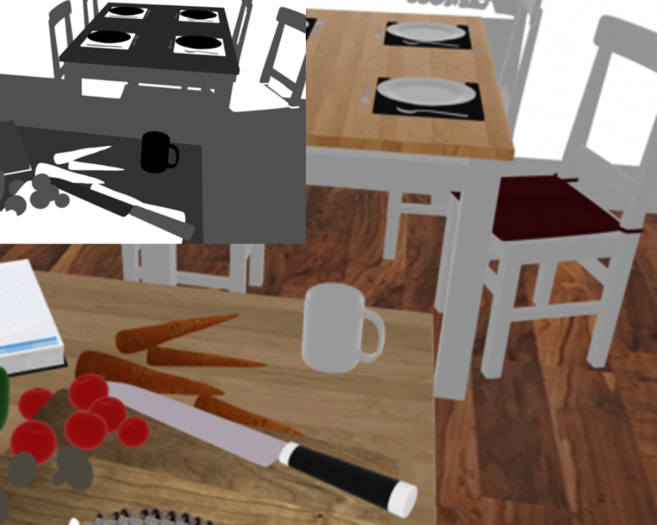
Positional encoding	Hash grid	Ground truth

Figure 15: Qualitative comparison of different input encoding shows a hash grid can better model the detailed texture on the floor.

Origin semantic segmentation		Fused semantic segmentation

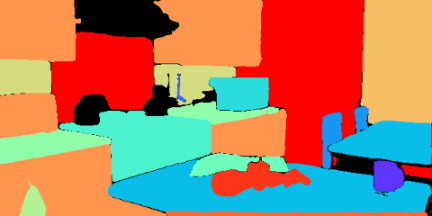
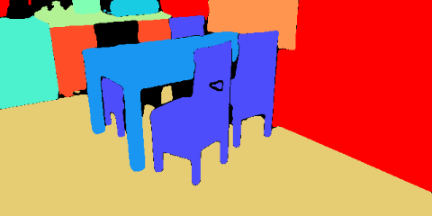
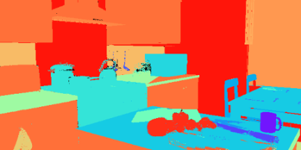
Figure 16: Fusing segmentation on raw images onto the mesh produces multi-view consistent segmentation.

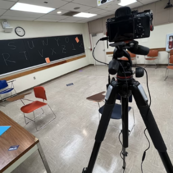
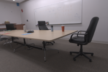
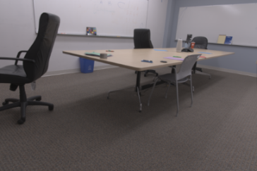
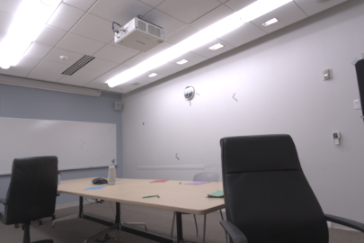
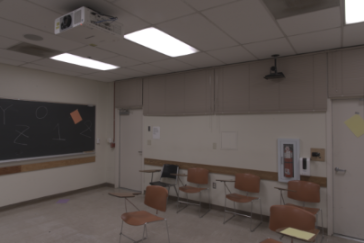
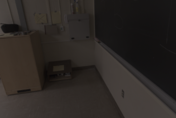
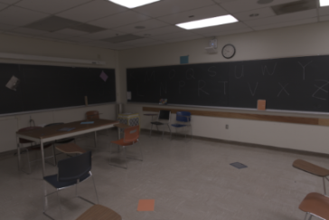
Conference room Classroom

Figure 17: The capture setting (left) and observations of the real world scenes (middle and right). We present two real world scenes (Conference room and Classroom) with samples of captured images, reconstructed geometries in 3 views, and all camera poses.

Appendix A Implementation Details

We implement our method in PyTorch [36] and Mitsuba 3 [15]. The diffuse and specular shadings in Eq. 6 are path-traced and denoised by the OptiX denoiser [35], where we use 128 samples per pixel for diffuse shadings and 64 for specular shadings. Importance sampling of the BRDF is applied for shading initialization (stage 1), and multiple importance sampling is applied for shading refinement (stage 3). For each round of BRDF-emission mask estimation (stage 2), the optimization is run over the entire training set for 2 epochs using Adam [20] optimizer with a learning rate of 1e-3 and a batch size of 8,192. Stage 2 and 3 are repeated twice after stage 1, and all the experiments are run on a single 3090Ti GPU.

Network architecture.

The BRDF network $\text{MLP}_{\text{brdf}}$ has 2 hidden layers of size 64, and its hash encoding [31] has 32 levels and 19 $\log_{2}$ hash map size with other parameters set to their recommended defaults. For emission mask network $\text{MLP}_{\text{emit}}$, we use positional encoding [30] with 10 frequency bands, 6 hidden layers of size 128, and one residual connection in the middle. Hash encoding is preferred for the BRDF network as albedo usually demonstrates high frequency pattern, which can be more efficiently modeled by a hash grid (Fig. 15). Both networks use ReLU activation between the intermediate layers.

Semantic segmentation acquisition.

To obtain semantic segmentation, we use Mask2Former [11] pre-trained on the COCO dataset [28] with Swin-L backbone. The input images are firstly tone-mapped with $\gamma=1/2.2$ then clipped to be in the range $[0,1]$. Given segmentation from multi-view images, we fuse them onto the mesh and let each mesh triangle take the segmentation ID with the maximum occurrence (Fig. 16).

Geometry acquisition with MonoSDF [53].

We adapt the original code from MonoSDF in the default configuration for ScanNet with Multi-Resolutional Feature Grids architecture and the following changes: (1) instead of having all rays coming from one image in each training iteration, we randomly sample over all training pixels, which is empirically found to yield more stable convergence on noisy inputs especially for real world images; (2) input images are changed from SDR to HDR to be in the same format as our model input; accordingly, output activation of MLP is changed to ReLU, and re-rendering loss is changed to L1 loss on tone-mapped outputs and labels. Considering MonoSDF does not incorporate an outlier rejection algorithm, we employ a two-step training strategy to deal with the bad camera poses. We first train for one epoch to acquire a rough mesh and reproject the mesh onto all frames. Frames with significant misalignment are then rejected and the model is re-trained. To extract the mesh, we employ Marching Cubes with a grid size of 512. In total, the entire process takes around 1 day per-scene.

Appendix B Experiment Details

B.1 Real world scene capture and relighting

Need for acquiring new real world data.

Existing datasets that provide multi-view HDR images and camera poses of real world scenes may include: Replica [45] , Matterport3D [10], and sample scenes from FVP [37]. However, each dataset has their own limitations that prohibit usage in our evaluation. Specifically, HDR images from FVP do not employ exposure bracketing, which results in overexposed emission that is not applicable to our physically-based light transport modeling. HDR images from Replica are not publicly available, thus view-dependent effects cannot be observed. For Matterport3D, the captured images exhibit artifacts including camera glare and problematic tone-mapping.

Therefore, we capture a few scenes as proof of concept of our method, including a conference room scene presented in the main paper and an additional classroom scene. Fig. 17 demonstrates our capture setting. We mount a Sony A7M3 full-frame camera on a tripod and use a remote control shutter release to capture images with exposure bracketing of 5 steps 1EV each or 5 steps 2EV each depending on the dynamic range of the room. We take images from multiple locations of the room, starting roughly with a direction towards the room center, then randomizing yaw angles between $-60\degree$ to $60\degree$, pitch angles between $-45\degree$ to $45\degree$, with minimal roll. The camera height is sampled between $0.5m$ to $2.5m$. For HDR reconstruction, we process the captured RAW images with black level subtraction, demosaicing, de-vignetting, and undistortion. The recovered images are assumed to follow linear camera response and are combined using a hat function similar to Debevec et al. [13].

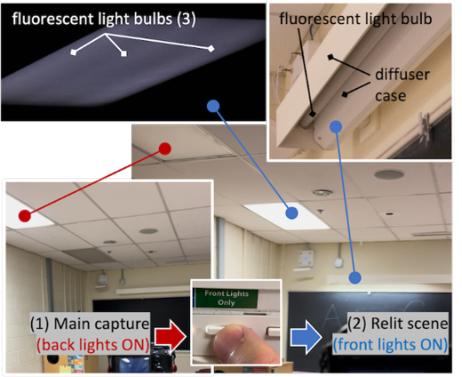
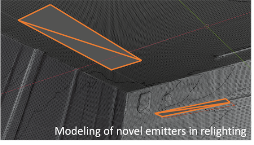
Figure 18: Relighting of the Classroom scene. The upper figure shows (1) the lighting for main captures with only back lights turned on, and (2) the relit scene with only front lights on (as reference for our relighting experiments). The lower figure shows our inserted area emitters as approximation of the actual front lights.

Reference relighting of Classroom.

As is shown in Fig. 18, lights in the Classroom can be switched between front and rear light modes. We choose the rear lights as original lighting for the main capture, and take a few additional photos with only front lights on as reference for relighting. Given BRDF-emission estimation from the main capture, we relight the scene by turning the estimated emission off and insert simple novel emitters to roughly match the front lights in their actual locations (see demonstration in Fig. 18, bottom). Considering it is not possible to have the manually inserted novel emitters to perfectly match the actual complex front lights, we treat the reference relighting photos only as pseudo-ground truth.

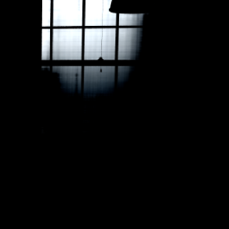
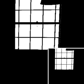
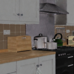
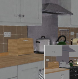
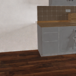
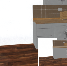
Joint vs separate $\mathbf{L}_{e}$ opt.		w/o vs w/ stage 3		w/o vs w/ rad. cache

Figure 19: Qualitative comparison of different training strategies shows all of the strategies are necessary for efficient and accurate BRDF-emission estimation. The insets are the ground truth.

Estimated geometry		Ground truth geometry
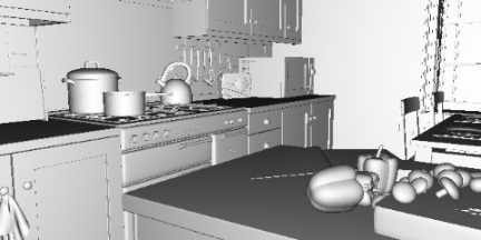
Semantic segmentation		Part segmentation
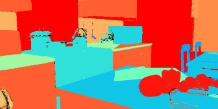
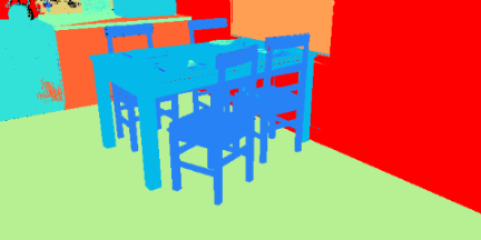
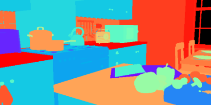
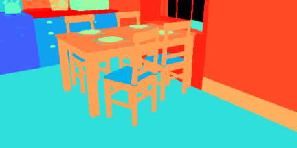
w/ estimated geometry
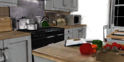
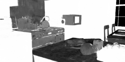
w/ semantic segmentation
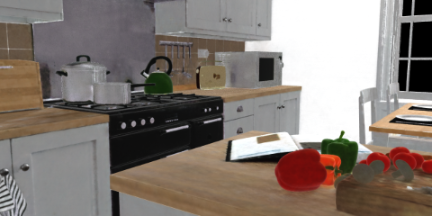
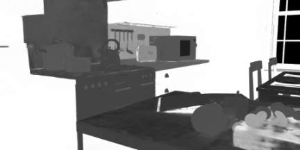
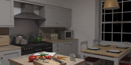
w/ ground truth geometry and part segmentation
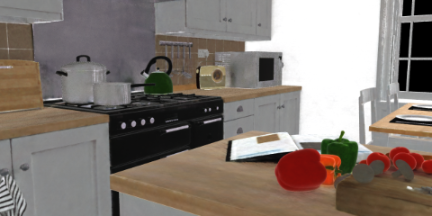
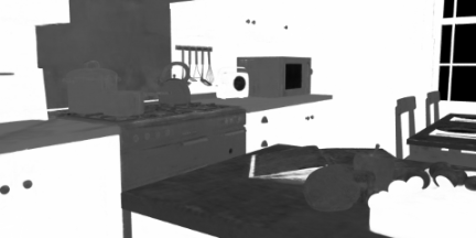
Ground truth

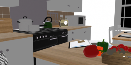
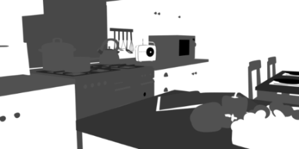
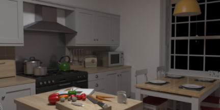
Figure 20: Sensitivity analysis on training inputs. Imperfect geometry and the usage of semantic segmentation instead of fine-grained part segmentation (row 1-2) can be acceptable for our BRDF-emission estimation (row 3-4, column 1-2). Ambiguity in roughness increases as geometry is imperfect or coarser segmentation is used (row 3-4, column 2), but they do not significantly affect applications like relighting (row 3-4, column 4).

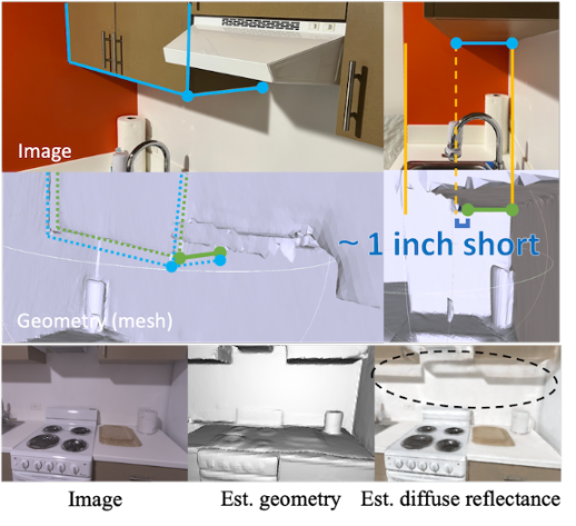
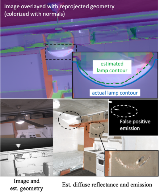
Figure 21: Failure cases of our method due to bad geometry. Top: indented cupboard (actual boundary in blue; estimated in green which has a geometry error of around 1 inch) results in incorrect light-surface intersection and boundary artifacts on the diffuse reflectance map (circled). Bottom: emission and bright artifacts (for diffuse reflectance) get erroneously baked onto the wall and cupboard (circled) because of the missing geometry on the lamp.

B.2 Ablation study details

Fig. 19 shows the effect of different training strategies on BRDF-emission estimation as discussed in Sec. 5.4. To demonstrate the impact of noisy inputs, Fig. 20 shows the quality of estimated geometry and semantic segmentation with respect to their ground truth together with the corresponding reconstruction results. It can be seen that surface roughness for regions with weak highlights can be very sensitive to inputs, while emission and material reflectance estimation are robust as long as the noise stays in a reasonable range.

Failure cases.

As discussed in the limitation section (Sec. 6), broken geometry can lead to large artifacts in our BRDF-emission reconstruction. A dormitory scene capture is shown in Fig. 21 to demonstrate the problem, where the front face of the reconstructed wall cabinet fails to align with the actual geometry (because of insufficient view coverage), causing the shadow boundary to be baked into the reflectance map. Meanwhile, geometry of the lamp on the ceiling fan is partly missing, which causes the emission to be incorrectly projected to the background wall and cabinet surface, creating bright artifacts on the reflectance map and phantom emitters on the wall.

B.3 Additional results

In Fig. 22, 23, we show the per-scene qualitative comparison of estimated BRDF and emission for all methods on synthetic dataset, and we compare the view synthesis and relighting results in Fig. 24, 25. In Fig. 26 and Fig. 27, we provide evaluation on additional views of our real world captures.

B.4 Evaluation scheme of baseline methods

For FVP [37], We use its original code with the following adaptations: FVP relies on thresholding RGB values to locate emitters, so we pick the threshold that separates emitters from the rest of the scene in our images. It also involves a step to manually set the exposure of each overexposed emitter, which in our adaptation is provided as the median radiance within each emitter. In relighting, FVP assumes the maximum radiance of novel emitters to be 1 so as to yield shading in SDR for input into its network. Afterwards, the exposure of novel emitters can be set to arbitrary numbers in FVP’s GUI. We follow the strategy but set exposure as our desired radiance values for novel emitters, so that relighting results from FVP can be directly comparable.

For evaluation of IPT [1] and MILO [51], since their code is not available, and a re-implementation requires careful design choices, we depend on results provided by the authors of MILO and IPT on our data, where it was possible for them to evaluate. Because MILO and FVP use texture-based representations, geometry is remeshed to prevent artifacts like UV seam and bleeding, which gives equivalent quality in most of the cases except for thin structures like disks on the kitchen table.

For Li22 [24], instead of using predicted depth, we directly back-project ground truth geometry to obtain a depth image as its input. On real scenes, considering the method is based on single-view input and does not allow rerendering to novel views under different lighting, we directly feed the reference relighting image as the input, replace all estimated emitters by our novel eimtters (Sec. B.1), and re-render the scene with estimated materials using its neural rendering pipeline.

Kitchen
MILO [51]	IPT [1]	Li22 [24]	NeILF [50]	FIPT (Ours)	FIPT-sem (Ours)	Ground truth
Bathroom

Figure 22: BRDF and emission estimation on synthetic Kitchen and Bathroom for all methods. Input views are shown in the upper-right corner of each scene.

Bedroom
MILO [51]	IPT [1]	Li22 [24]	NeILF [50]	FIPT (Ours)	FIPT-sem (Ours)	Ground truth
Livingroom

Figure 23: BRDF and emission estimation results on synthetic Bedroom and Livingroom for all methods, showing 2 views per-scene. Input views are shown in the upper-right corner of each scene.

Kitchen
MILO [51]	IPT [1]	FVP [37]	FIPT (Ours)	FIPT-sem (Ours)	Ground truth
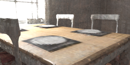
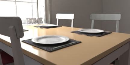
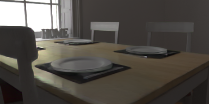
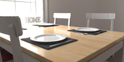
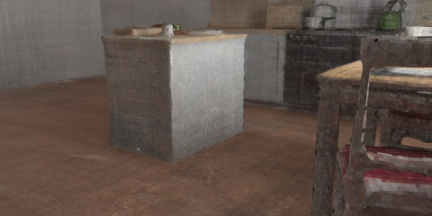
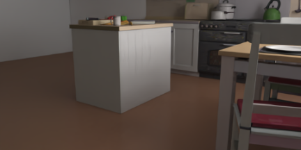
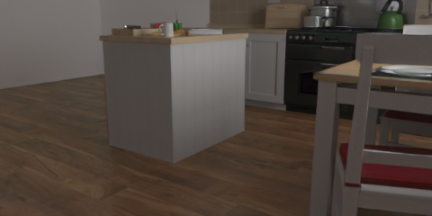
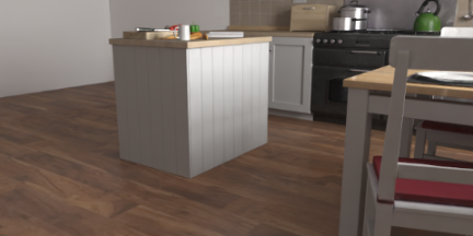
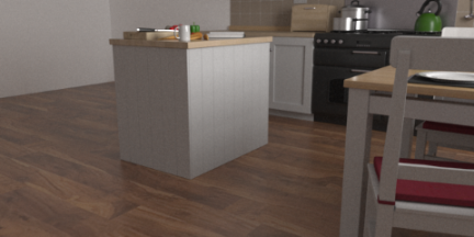
Bathroom
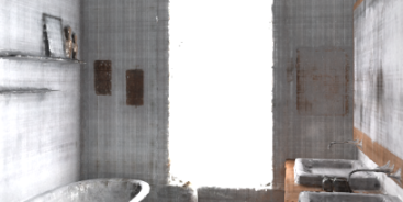
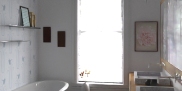
Bedroom
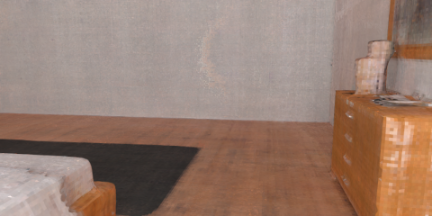
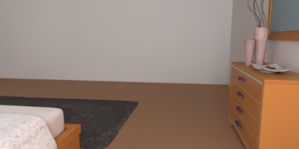
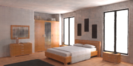
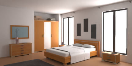
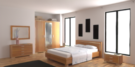
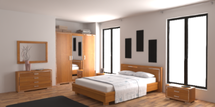
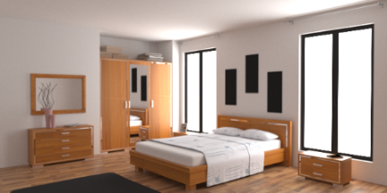
Livingroom

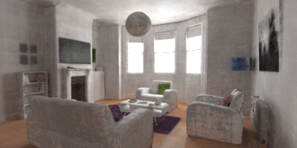
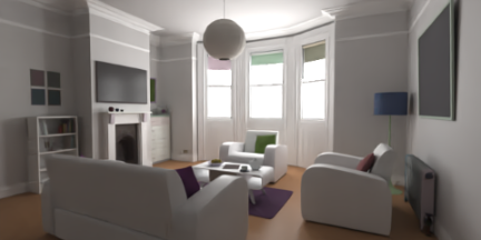
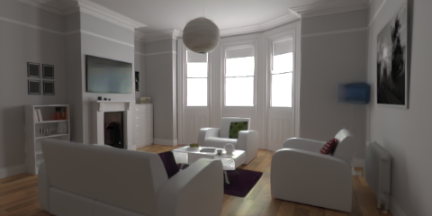
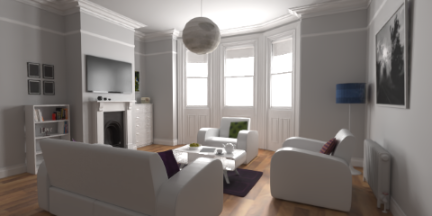
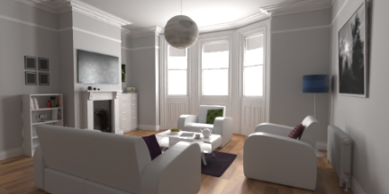
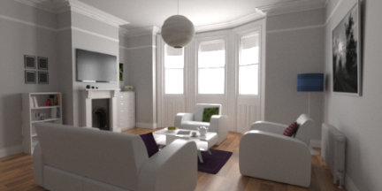
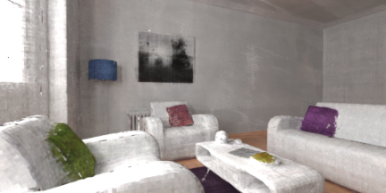
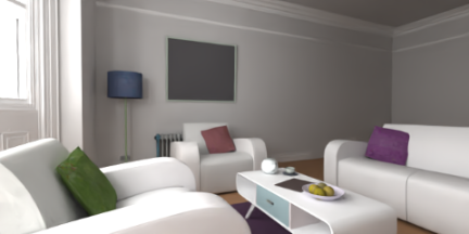
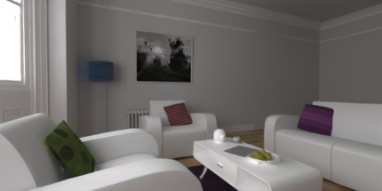
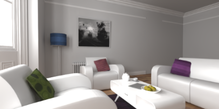
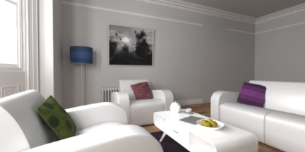
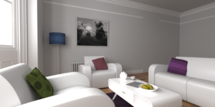
Figure 24: View synthesis results on synthetic scenes for all methods, showing 2 views per-scene.

Kitchen
MILO [51]	IPT [1]	Li22 [24]	FVP [37]	FIPT (Ours)	FIPT-sem (Ours)	Ground truth
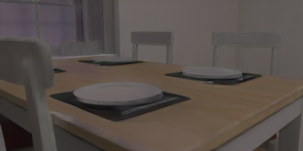
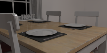
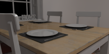
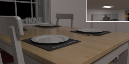
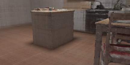
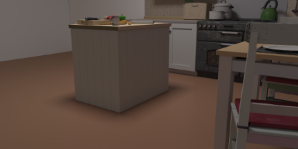
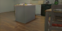
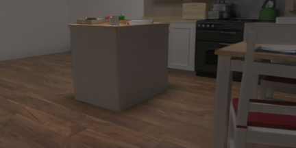
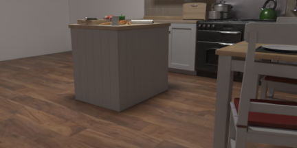
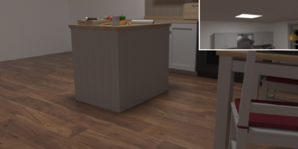
Bathroom
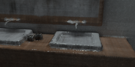
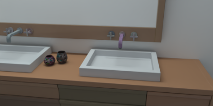
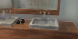
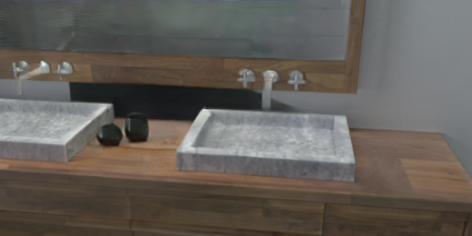
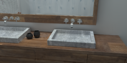
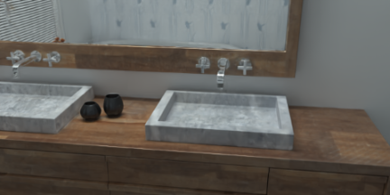
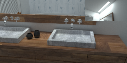
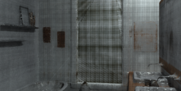
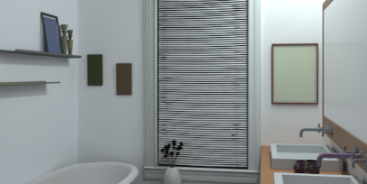
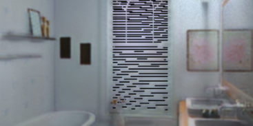
Bedroom
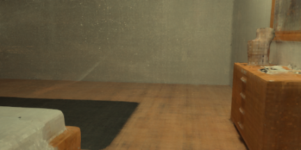
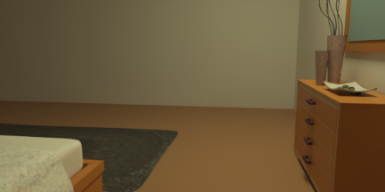
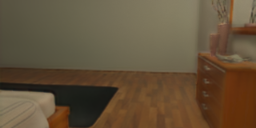
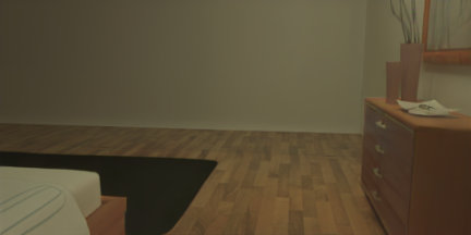
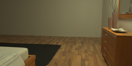
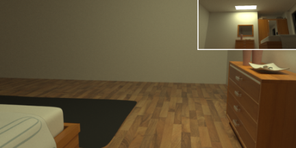
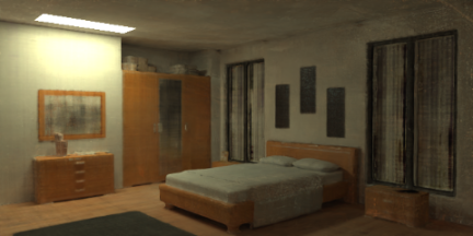
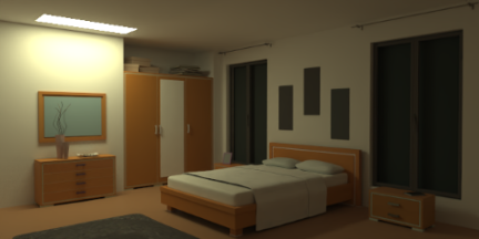
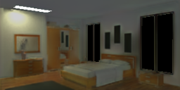
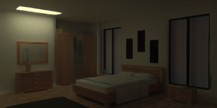
Livingroom

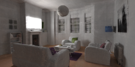
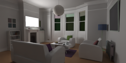
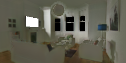
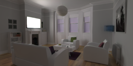
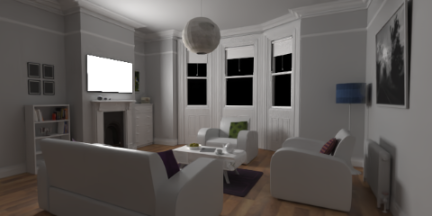
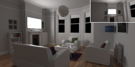
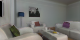
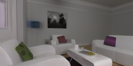
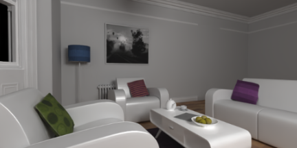
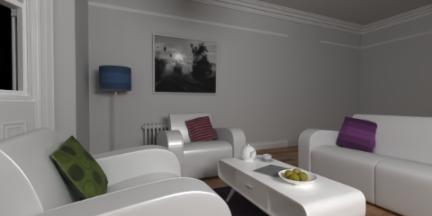
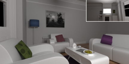
Figure 25: Relighting results on synthetic scenes for all methods, showing 2 views per-scene.

Conference room			Classroom
MILO [51]	Li22 [24]	FIPT (Ours)	MILO [51]	Li22 [24]	FIPT (Ours)	Reference

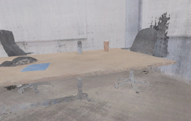
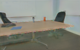
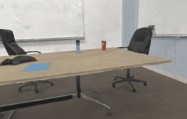
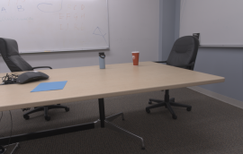
Figure 26: BRDF and emission estimation on real scenes, showing 1 additional view per-scene besides views shown in the main paper.

Conference room
MILO [51]	Li22 [24]	FVP [37]	FIPT (Ours)	Ground Truth
Classroom
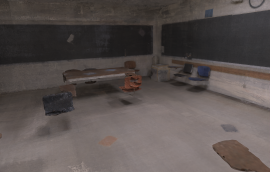
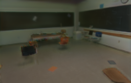
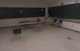
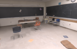
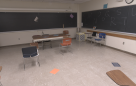
Rerendering
Conference room
MILO [51]	Li22 [24]	FVP [37]	FIPT (Ours)	Reference
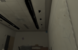
Classroom
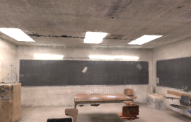
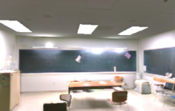
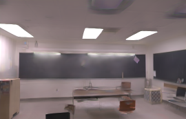
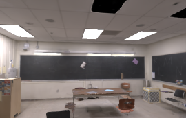
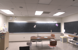
Relighting

Figure 27: Rerendering and relighting on real scenes, showing 1 additional view per-scene for each task besides views shown in the main paper. Top two rows show the rerendering with original lighting (Conference room: all ceiling lamps on; Classroom: rear lights on and fronts lights off). Bottom two rows show the relighting under novel light with relit Classroom also included as pseudo-ground truth (with rear lights off, and front lights on).

References

- [1] Dejan Azinovic, Tzu-Mao Li, Anton Kaplanyan, and Matthias Nießner. Inverse path tracing for joint material and lighting estimation. In CVPR, 2019.
- [2] Sai Praveen Bangaru, Michaël Gharbi, Fujun Luan, Tzu-Mao Li, Kalyan Sunkavalli, Milos Hasan, Sai Bi, Zexiang Xu, Gilbert Louis Bernstein, and Frédo Durand. Differentiable rendering of neural sdfs through reparameterization. In SIGGRAPH Asia, 2022.
- [3] Sai Praveen Bangaru, Tzu-Mao Li, and Frédo Durand. Unbiased warped-area sampling for differentiable rendering. In ACM Transactions on Graphics (TOG), volume 39, pages 1–18, 2020.
- [4] Jonathan T Barron and Jitendra Malik. Intrinsic scene properties from a single rgb-d image. In Proceedings of the IEEE Conference on Computer Vision and Pattern Recognition, pages 17–24, 2013.
- [5] Benedikt Bitterli. Rendering resources, 2016. https://benedikt-bitterli.me/resources/.
- [6] Blender Online Community. Blender - a 3d modelling and rendering package, 2022.
- [7] Mark Boss, Raphael Braun, Varun Jampani, Jonathan T Barron, Ce Liu, and Hendrik Lensch. Nerd: Neural reflectance decomposition from image collections. In ICCV, pages 12684–12694, 2021.
- [8] Mark Boss, Varun Jampani, Raphael Braun, Ce Liu, Jonathan Barron, and Hendrik Lensch. Neural-pil: Neural pre-integrated lighting for reflectance decomposition. In NeurIPS, volume 34, pages 10691–10704, 2021.
- [9] Brent Burley and Walt Disney Animation Studios. Physically-based shading at disney. In SIGGRAPH, volume 2012, pages 1–7. vol. 2012, 2012.
- [10] Angel Chang, Angela Dai, Thomas Funkhouser, Maciej Halber, Matthias Niebner, Manolis Savva, Shuran Song, Andy Zeng, and Yinda Zhang. Matterport3d: Learning from rgb-d data in indoor environments. In 3DV, pages 667–676, 2018.
- [11] Bowen Cheng, Ishan Misra, Alexander G. Schwing, Alexander Kirillov, and Rohit Girdhar. Masked-attention mask transformer for universal image segmentation. In CVPR, 2022.
- [12] Paul Debevec. Rendering synthetic objects into real scenes: Bridging traditional and image-based graphics with global illumination and high dynamic range photography. In SIGGRAPH, page 189–198, 1998.
- [13] Paul E Debevec and Jitendra Malik. Recovering high dynamic range radiance maps from photographs. In ACM SIGGRAPH 2008 classes, pages 1–10, 2008.
- [14] Marc-André Gardner, Kalyan Sunkavalli, Ersin Yumer, Xiaohui Shen, Emiliano Gambaretto, Christian Gagné, and Jean-François Lalonde. Learning to predict indoor illumination from a single image. ACM Transactions on Graphics (TOG), 36(6):1–14, 2017.
- [15] Wenzel Jakob, Sébastien Speierer, Nicolas Roussel, Merlin Nimier-David, Delio Vicini, Tizian Zeltner, Baptiste Nicolet, Miguel Crespo, Vincent Leroy, and Ziyi Zhang. Mitsuba 3 renderer, 2022. https://mitsuba-renderer.org.
- [16] James T Kajiya. The rendering equation. In SIGGRAPH, pages 143–150, 1986.
- [17] Brian Karis. Real shading in unreal engine 4. In SIGGRAPH 2013 Course: Physically Based Shading in Theory and Practice, 2013.
- [18] Kevin Karsch, Varsha Hedau, David Forsyth, and Derek Hoiem. Rendering synthetic objects into legacy photographs. ACM Transactions on Graphics (TOG), 30(6):1–12, 2011.
- [19] Kevin Karsch, Kalyan Sunkavalli, Sunil Hadap, Nathan Carr, Hailin Jin, Rafael Fonte, Michael Sittig, and David Forsyth. Automatic scene inference for 3d object compositing. ACM Transactions on Graphics (TOG), 33(3):1–15, 2014.
- [20] Diederik P Kingma and Jimmy Ba. Adam: A method for stochastic optimization. arXiv preprint arXiv:1412.6980, 2014.
- [21] Jaroslav Křivánek, Pascal Gautron, Greg Ward, Okan Arikan, and Henrik Wann Jensen. Practical global illumination with irradiance caching. In ACM SIGGRAPH 2007 courses, 2007.
- [22] Tzu-Mao Li, Miika Aittala, Frédo Durand, and Jaakko Lehtinen. Differentiable monte carlo ray tracing through edge sampling. In ACM Transactions on Graphics (TOG), volume 37, pages 1–11, 2018.
- [23] Zhengqin Li, Mohammad Shafiei, Ravi Ramamoorthi, Kalyan Sunkavalli, and Manmohan Chandraker. Inverse rendering for complex indoor scenes: Shape, spatially-varying lighting and svbrdf from a single image. In CVPR, 2020.
- [24] Zhengqin Li, Jia Shi, Sai Bi, Rui Zhu, Kalyan Sunkavalli, Miloš Hašan, Zexiang Xu, Ravi Ramamoorthi, and Manmohan Chandraker. Physically-based editing of indoor scene lighting from a single image. In ECCV, 2022.
- [25] Zhen Li, Lingli Wang, Mofang Cheng, Cihui Pan, and Jiaqi Yang. Multi-view inverse rendering for large-scale real-world indoor scenes. arXiv preprint arXiv:2211.10206, 2022.
- [26] Zhen Li, Lingli Wang, Mofang Cheng, Cihui Pan, and Jiaqi Yang. Multi-view inverse rendering for large-scale real-world indoor scenes. arXiv preprint arXiv:2211.10206, 2022.
- [27] Zhengqin Li, Zexiang Xu, Ravi Ramamoorthi, Kalyan Sunkavalli, and Manmohan Chandraker. Learning to reconstruct shape and spatially-varying reflectance from a single image. In ACM Trans. Graph. (Proc. SIGGRAPH Asia), volume 37, 2018.
- [28] Tsung-Yi Lin, Michael Maire, Serge Belongie, James Hays, Pietro Perona, Deva Ramanan, Piotr Dollár, and C Lawrence Zitnick. Microsoft coco: Common objects in context. In ECCV, pages 740–755, 2014.
- [29] Robert Maier, Kihwan Kim, Daniel Cremers, Jan Kautz, and Matthias Nießner. Intrinsic3d: High-quality 3d reconstruction by joint appearance and geometry optimization with spatially-varying lighting. In ICCV, pages 3114–3122, 2017.
- [30] Ben Mildenhall, Pratul P. Srinivasan, Matthew Tancik, Jonathan T. Barron, Ravi Ramamoorthi, and Ren Ng. Nerf: Representing scenes as neural radiance fields for view synthesis. In ECCV, 2020.
- [31] Thomas Müller, Alex Evans, Christoph Schied, and Alexander Keller. Instant neural graphics primitives with a multiresolution hash encoding. In ACM Transactions on Graphics (ToG), volume 41, pages 1–15, 2022.
- [32] Jacob Munkberg, Jon Hasselgren, Tianchang Shen, Jun Gao, Wenzheng Chen, Alex Evans, Thomas Müller, and Sanja Fidler. Extracting triangular 3d models, materials, and lighting from images. In CVPR, pages 8280–8290, 2022.
- [33] Merlin Nimier-David, Zhao Dong, Wenzel Jakob, and Anton Kaplanyan. Material and Lighting Reconstruction for Complex Indoor Scenes with Texture-space Differentiable Rendering. In Adrien Bousseau and Morgan McGuire, editors, Eurographics Symposium on Rendering - DL-only Track, 2021.
- [34] Merlin Nimier-David, Delio Vicini, Tizian Zeltner, and Wenzel Jakob. Mitsuba 2: A retargetable forward and inverse renderer. In ACM Trans. Graph. (Proc. SIGGRAPH Asia), volume 38, 2019.
- [35] Steven G Parker, James Bigler, Andreas Dietrich, Heiko Friedrich, Jared Hoberock, David Luebke, David McAllister, Morgan McGuire, Keith Morley, Austin Robison, et al. Optix: a general purpose ray tracing engine. In Acm transactions on graphics (tog), volume 29, pages 1–13, 2010.
- [36] Adam Paszke, Sam Gross, Francisco Massa, Adam Lerer, James Bradbury, Gregory Chanan, Trevor Killeen, Zeming Lin, Natalia Gimelshein, Luca Antiga, et al. Pytorch: An imperative style, high-performance deep learning library. In NeurIPS, volume 32, 2019.
- [37] Julien Philip, Sébastien Morgenthaler, Michaël Gharbi, and George Drettakis. Free-viewpoint indoor neural relighting from multi-view stereo. In ACM Transactions on Graphics (TOG), volume 40, pages 1–18, 2021.
- [38] Ravi Ramamoorthi and Pat Hanrahan. An efficient representation for irradiance environment maps. In SIGGRAPH, pages 497–500, 2001.
- [39] Christophe Schlick. An inexpensive brdf model for physically-based rendering. In Computer graphics forum, volume 13, pages 233–246. Wiley Online Library, 1994.
- [40] Johannes Lutz Schönberger, Enliang Zheng, Marc Pollefeys, and Jan-Michael Frahm. Pixelwise view selection for unstructured multi-view stereo. In ECCV, 2016.
- [41] Soumyadip Sengupta, Jinwei Gu, Kihwan Kim, Guilin Liu, David W Jacobs, and Jan Kautz. Neural inverse rendering of an indoor scene from a single image. In ICCV, pages 8598–8607, 2019.
- [42] Dario Seyb, Peter-Pike Sloan, Ari Silvennoinen, Michał Iwanicki, and Wojciech Jarosz. The design and evolution of the UberBake light baking system. In ACM Trans. Graph. (Proc. SIGGRAPH), volume 39, 2020.
- [43] Pratul P Srinivasan, Boyang Deng, Xiuming Zhang, Matthew Tancik, Ben Mildenhall, and Jonathan T Barron. Nerv: Neural reflectance and visibility fields for relighting and view synthesis. In CVPR, pages 7495–7504, 2021.
- [44] Pratul P Srinivasan, Ben Mildenhall, Matthew Tancik, Jonathan T Barron, Richard Tucker, and Noah Snavely. Lighthouse: Predicting lighting volumes for spatially-coherent illumination. In CVPR, pages 8080–8089, 2020.
- [45] Julian Straub, Thomas Whelan, Lingni Ma, Yufan Chen, Erik Wijmans, Simon Green, Jakob J Engel, Raul Mur-Artal, Carl Ren, Shobhit Verma, et al. The replica dataset: A digital replica of indoor spaces. arXiv preprint arXiv:1906.05797, 2019.
- [46] Delio Vicini, Sébastien Speierer, and Wenzel Jakob. Differentiable signed distance function rendering. In ACM Transactions on Graphics (TOG), volume 41, pages 1–18, 2022.
- [47] Bruce Walter, Stephen R Marschner, Hongsong Li, and Kenneth E Torrance. Microfacet models for refraction through rough surfaces. In Eurographics conference on Rendering Techniques, pages 195–206, 2007.
- [48] Zian Wang, Jonah Philion, Sanja Fidler, and Jan Kautz. Learning indoor inverse rendering with 3d spatially-varying lighting. In ICCV, pages 12538–12547, 2021.
- [49] Gregory J. Ward, Francis M. Rubinstein, and Robert D. Clear. A ray tracing solution for diffuse interreflection. In SIGGRAPH, pages 85–92, 1988.
- [50] Yao Yao, Jingyang Zhang, Jingbo Liu, Yihang Qu, Tian Fang, David McKinnon, Yanghai Tsin, and Long Quan. Neilf: Neural incident light field for physically-based material estimation. In ECCV, pages 700–716, 2022.
- [51] Bohan Yu, Siqi Yang, Xuanning Cui, Siyan Dong, Baoquan Chen, and Boxin Shi. Milo: Multi-bounce inverse rendering for indoor scene with light-emitting objects. In IEEE Transactions on Pattern Analysis and Machine Intelligence, 2023.
- [52] Yizhou Yu, Paul Debevec, Jitendra Malik, and Tim Hawkins. Inverse global illumination: Recovering reflectance models of real scenes from photographs. In SIGGRAPH, pages 215–224, 1999.
- [53] Zehao Yu, Songyou Peng, Michael Niemeyer, Torsten Sattler, and Andreas Geiger. Monosdf: Exploring monocular geometric cues for neural implicit surface reconstruction. In NeurIPS, 2022.
- [54] Tizian Zeltner, Sébastien Speierer, Iliyan Georgiev, and Wenzel Jakob. Monte Carlo estimators for differential light transport. In ACM Trans. Graph. (Proc. SIGGRAPH), volume 40, 2021.
- [55] Kai Zhang, Fujun Luan, Qianqian Wang, Kavita Bala, and Noah Snavely. Physg: Inverse rendering with spherical gaussians for physics-based material editing and relighting. In CVPR, pages 5453–5462, 2021.
- [56] Xiuming Zhang, Pratul P Srinivasan, Boyang Deng, Paul Debevec, William T Freeman, and Jonathan T Barron. Nerfactor: Neural factorization of shape and reflectance under an unknown illumination. In ACM Transactions on Graphics (TOG), volume 40, pages 1–18, 2021.
- [57] Rui Zhu, Zhengqin Li, Janarbek Matai, Fatih Porikli, and Manmohan Chandraker. Irisformer: Dense vision transformers for single-image inverse rendering in indoor scenes. In CVPR, pages 2822–2831, 2022.