Evidence of experimental three-wave resonant interactions
between two dispersion branches

Abstract

We report the observation of nonlinear three-wave resonant interactions between two different branches of the dispersion relation of hydrodynamic waves, namely the gravity-capillary and sloshing modes. These atypical interactions are investigated within a torus of fluid for which the sloshing mode can be easily excited. A triadic resonance instability is then observed due to this three-wave two-branch interaction mechanism. An exponential growth of the instability and phase locking are evidenced. The efficiency of this interaction is found to be maximal when the gravity-capillary phase velocity matches the group velocity of the sloshing mode. For a stronger forcing, additional waves are generated by a cascade of three-wave interactions populating the wave spectrum. Such a three-wave two-branch interaction mechanism is probably not restricted to hydrodynamics and could be of interest in other systems involving several propagation modes.

I Introduction

Nonlinear wave interactions occur in a variety of systems, where waves of different wavenumbers and frequencies can exchange energy through nonlinear couplings. Such interactions also form the basis for wave-turbulent regimes, where a whole ensemble of waves with different wavenumbers interact among each other and can exhibit a cascade of energy from large to small scales [1].

The case of three-wave interactions is prevalent in many areas, such as plasma physics [2, 3], nonlinear optics [4], Rossby waves [5], and even mechanical systems such as suspended cables [6] or thin rings [7]. For hydrodynamic surface waves, three-wave interactions have been extensively studied in the case of gravity-capillary waves [8, 9] and hydroelastic waves [10]. In the case of gravity waves, four-wave interactions dominate [11, 12]. However, considering one-dimensional (1D) deep-water propagation leads at the leading order to five-wave resonant interactions for either pure capillary waves [13] or pure gravity waves [14, 15].

Three-wave systems can also be the source of instability [16]. Depending on the nonlinear coupling between the three waves, a single “mother” wave can give rise to two “daughter” waves, that then grow exponentially in amplitude. The waves of this triadic resonant instability (TRI) satisfy both resonances in wavenumber and frequency and has been widely observed in internal waves in stratified flows [17, 18, 19], as well as in inertial waves [20, 21] providing a potential route to wave turbulence [22, 23, 24, 25]. A special case of TRI is the parametric subharmonic instability, involving daughter waves with frequencies close to the first subharmonic of the mother wave and has been well investigated in areas such as plasma physics [26, 27] and oceanic systems [28].

Gravity-capillary waves on the two-dimensional surface of a fluid are well-known in both the linear regime [29] as well as the nonlinear wave-turbulent case [30, 31]. When one of the dimensions of the system is much smaller than the other, for example in canals, sloshing waves become apparent [29, 32], and lead to longitudinal waves with associated discrete transverse modes. This results in a countably infinite number of branches in the dispersion relation, each corresponding to one of the transverse modes, similar to modes of waveguides [33].

The sloshing modes can theoretically trigger nonlinear interactions between waves belonging to different branches of the dispersion relation [34]. However, the study of the interaction between nonlinear waves of different types (i.e., belonging to separate branches) has not been investigated experimentally so far. Such an unexplored interaction mechanism could potentially be applicable in various domains such as two-component systems  [35, 36], atomic lattices [37], or plasma physics [38]. Such multiple branch dispersion relations are also characteristic of waves in waveguides, for example in solid and soft plates [33]. Besides, it provides a way to test wave turbulence in media where multiple wave species are present [39] and bears a similarity to interactions between interfacial and free-surface waves [40, 41].

Here, we will study the interaction between gravity-capillary waves and the first sloshing mode. To the best of our knowledge, such three-wave interactions have not been considered experimentally which is possibly due to the difficulty of cleanly exciting sloshing modes in typical experiments. The system under study is a torus of fluid, which has been shown to contain multiple modes of propagation, including sloshing [42], but also easily demonstrates nonlinear behavior, as shown in the case of Korteweg-de Vries (KdV) solitons [43]. Because of its relatively small size ($R\approx 8$ cm), the torus is easy to manipulate and excite.

The paper is organized as follows. First, we describe in Sec. II the experimental setup and the different branches of the dispersion relation. Section III will then present the experimental results related to the three-wave two-branch interaction. In particular, the sloshing branch can trigger a triadic resonant instability, generating two gravity-capillary waves, for which the wave growth rate and phase locking are characterized. The efficiency of this mechanism is shown to be mediated by a velocity matching between the two types of propagation modes. Finally, Sec. IV draws the conclusions.

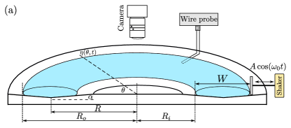
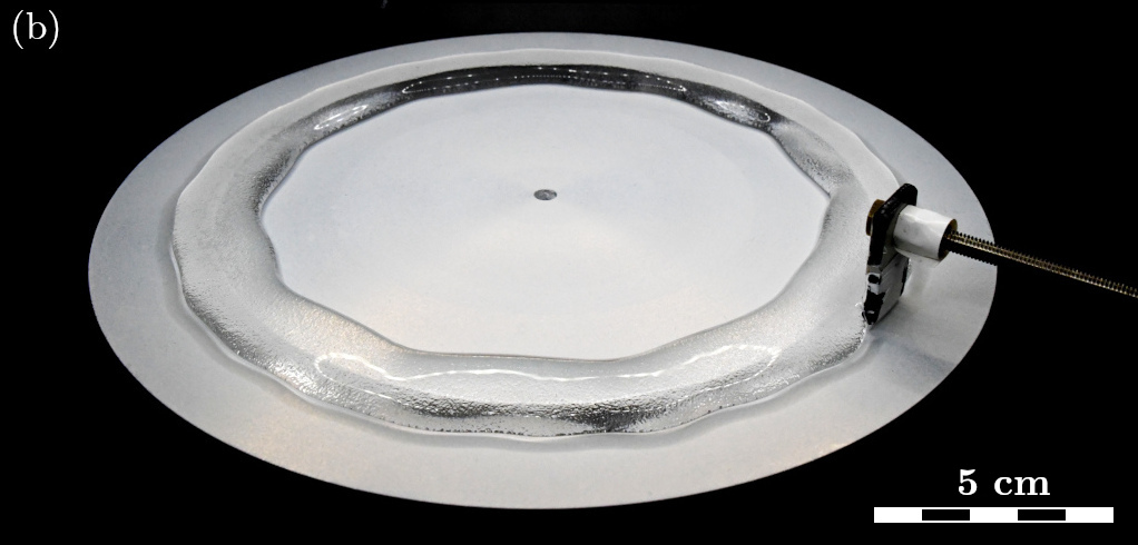
Figure 1: (a) Cross-section of the experimental setup with relevant quantities. (b) Side-view of the torus ($R_{0}=7.85$ cm) under monochromatic excitation, $f_{0}=7.4$ Hz.

II The torus of fluid

II.1 Experimental setup

The experimental setup used is the same as the one described in Ref. [42]. The torus of fluid is formed by depositing distilled water on top of a circular plate that has been coated with a commercial superhydrophobic treatment. The plate has a triangular groove running along its perimeter, as is shown in Fig. 1a. The angle of the groove is $\alpha=4.5\degree$. It prevents the closing of the central hole of the torus due to capillarity.

The waves are created by a Teflon plate connected to an electromagnetic shaker with adjustable sinusoidal amplitude and frequency typically in the range $7$-$9$ Hz [see Fig. 1b]. The waves propagate azimuthally on both the inner and outer borders of the torus. The waves also experience dissipation, which is primarily due to friction of the triple contact line, and not necessarily viscosity [43]. The motion of the border of the torus is captured by a camera located directly above the plate. By using a contour extraction algorithm we obtain the displacement $\eta(\theta,t)$ of the borders. We will be focusing on the motion of the outer border unless otherwise mentioned. The second method of detecting the border displacement is through the use of a custom-made local capacitive wire probe, giving the position of the outer border over time at a fixed azimuthal point $\theta_{0}$ with a high temporal resolution ($2$ kHz) [see Fig. 1a]. The central radius of the groove of the plate is $R=7$ cm, while the torus size is fixed at the outer border radius $R_{o}=7.85$ cm. The torus width is then fixed to $W=R_{o}-R_{i}=2(R_{o}-R)=1.7$ cm.

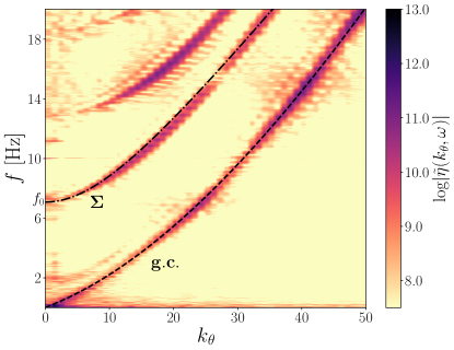
Figure 2: Space-time Fourier spectrum $\tilde{\eta}(k_{\theta},f)$ of the outer border displacement $\eta(\theta,t)$ on a torus of fluid, $R_{o}=7.85$ cm. Forcing: frequency sweep between $0$ and $20$ Hz on the outer border. Dashed lines: fit of the gravity-capillary dispersion relation (gc) of Eq. (1), and of the sloshing branch, $\Sigma$, given by Eq. (2).

II.2 Dispersion relation and resonant interaction

The torus admits several modes of wave propagation such as gravity-capillary azimuthal waves and sloshing modes [42]. Using a sweep forcing, the experimental Fourier spectrum $\tilde{\eta}(k_{\theta},f)$ of the outer border displacement $\eta(\theta,t)$ is shown in Fig. 2 highlighting the gravity-capillary and sloshing branches.

The dispersion relation of gravity-capillary waves is found to be empirically well described by [42]

$$\omega^{2}_{\mathrm{gc}}=\left(g_{\mathrm{eff}}\frac{k_{\theta}}{R_{o}}+\frac{\sigma_{\mathrm{eff}}}{\rho}\frac{k_{\theta}^{3}}{R_{o}^{3}}\right)\tanh{\left(\frac{k_{\theta}}{R_{o}}\chi^{2}\widetilde{W}\right)}{\rm\,,}$$ (1)

with $\widetilde{W}=W/2$ the half-width, $\chi=R_{o}/R$ a measure of curvature, $\rho=1000$ kg$/$m³ the density of the fluid, and $k_{\theta}$ the angular integer wavenumber, i.e., the discrete mode number which is given as $k_{\theta}=kR_{o}$, with $k$ the dimensional wavenumber of a wave traveling along the torus border. Since the waves are moving on a slope, they experience an effective gravity which is given by $g_{\mathrm{eff}}=g\sin\alpha\approx 0.77\,\textup{ms}^{-2}$. The effective surface tension is inferred from fitting the dispersion relation as $\sigma_{\mathrm{eff}}=55$ mN$/$m. This low value is due to the channel geometry and renormalization effects [44].

Alongside the gravity-capillary branch, we consider the first sloshing mode, also given empirically as [42]

$$\omega_{\Sigma}^{2}=\omega_{0}^{2}+g_{\mathrm{eff}}\frac{k_{\theta}^{2}}{R}{\rm\,,}$$ (2)

for values of $k_{\theta}\lesssim 40$, where $\omega_{0}$ is the cutoff frequency at $k_{\theta}=0$. This relationship includes only gravity, and for higher frequencies surface tension needs to be taken into account. In the present work, we will assume that the relationship is a good approximation at the low wavenumbers we consider here.

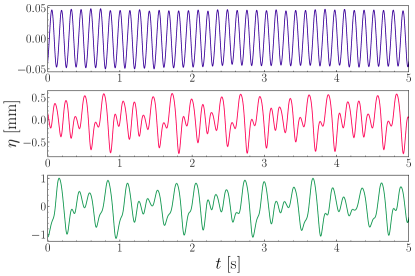
Figure 3: Displacement $\eta(t)$ at a fixed point for three different amplitudes of forcing ($f_{1}=7.4$ Hz) increasing from top to bottom with the corresponding values of wave steepness $\epsilon=0.003$, 0.02, and 0.03. The signal goes from a sine wave into a superposition of various subharmonics.

We now turn to the nonlinear interactions between waves. Waves are capable of exchanging energy through nonlinear resonant interactions if they satisfy the conservation of both frequency and wavenumber, which in the case of three waves are

$$\begin{split}k_{1}&=k_{2}+k_{3}{\rm\,,}\\ \omega_{1}&=\omega_{2}+\omega_{3}{\rm\,,}\end{split}$$ (3)

with $\omega_{i}=\omega(|k_{i}|)$, $\omega(k)$ being the dispersion relation of the considered system. The above equations can be solved once the dispersion relation of the waves is provided. In addition, the involved waves do not need to be of the same type and may belong to different dispersion branches. Depending on the studied system, solutions of Eq. (3) can also give only trivial solutions which do not lead to an exchange of energy. We will be interested in studying the interaction of the two different modes mentioned above i.e., between the first two branches in Fig. 2 (namely the gravity-capillary and first sloshing branch) and whether they satisfy the conditions given by Eq. (3).

III Experimental observations

III.1 Triadic instability

A monochromatic signal is sent to the shaker at a frequency of $f_{1}=\omega_{1}/2\pi$. We measure the displacement of the outer border $\eta(t)$ at a fixed point for three different amplitudes of forcing as shown in Fig. 3

At low forcing, $\eta(t)$ very closely resembles a sine wave. By increasing the amplitude, $\eta(t)$ changes significantly, indicating the existence of a critical forcing amplitude and seems to become a superposition of multiple different frequencies, while still preserving some quasi-periodicity.

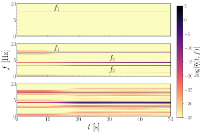
Figure 4: Time-frequency spectrum of the wave amplitudes of Fig. 3. For low forcing, a single frequency is present, $f_{1}=7.4$ Hz (top), but for a high enough forcing, two frequencies appear at $f_{2}=4.2$ Hz and $f_{3}=3.2$ Hz (middle). Further increase of the forcing generates an ensemble of different modes (bottom).

We compute the time-frequency spectrum of $\eta(t)$ (also called spectrograms) to distinguish the frequency components contained in the signal, as shown in Fig. 4 for the three forcing amplitudes. For a low forcing, a single frequency is found, corresponding precisely to the forcing one, $f_{1}$. As the forcing is increased, two additional subharmonic frequencies appear, neither of which is located at $f_{1}/2$. This behavior is characteristic of the triadic resonant instability, where, by forcing the system at a given pump frequency $f_{1}$, two subharmonic waves, $f_{2}$ and $f_{3}$ are pumped up from zero amplitude and thus begin to deplete the pump. It is worth noting that the sum of these two new frequencies, $f_{2}$ and $f_{3}$ equals $f_{1}$. We also see that a typical time (of the order of $10$ s) is necessary for these waves to be established in the spectrum. As the amplitude of forcing is increased further, additional frequencies besides the first pair become visible but take more time to appear, and they do so after the original pair is established.

III.2 Resonance conditions

To verify that the signals we observe are due to a resonant three-wave interaction, we first consider the spatiotemporal signal of the torus outer border $\eta(\theta,t)$. We then compute the corresponding space and time Fourier transform $\tilde{\eta}(k_{\theta},\omega)$ as shown in Fig. 5. It gives us not only the frequency but also wavenumber information of the waves present in the system. Figure 5 shows that the pumping frequency $f_{1}$ excited the sloshing branch, and the corresponding part on the gravity-capillary branch, but also two lower frequency points, $f_{2}$ and $f_{3}$ on the gravity-capillary branch. Note that the discreteness in $k_{\theta}$ is due to the torus finite size, whereas the one in $f$ corresponds to the inverse of the total measurement time.

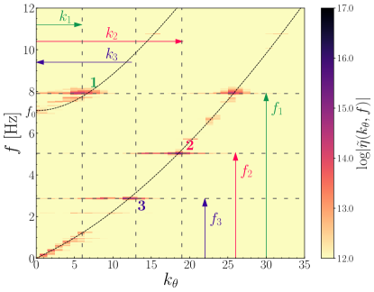
Figure 5: Fourier spectrum $\tilde{\eta}(k_{\theta},f)$ of the torus outer border displacement $\eta(\theta,t)$. Monochromatic forcing at $f_{1}=7.9$ Hz. Points $(k_{2},f_{2})$ and $(k_{3},f_{3})$ lie on the gravity-capillary branch whereas, point $(k_{1},f_{1})$ lies on the sloshing branch where it is forced. All three points verify the resonance conditions in both frequency and wavenumber (see arrows). $f_{0}$ is the cutoff frequency of the sloshing branch.

Thus, one has to consider the following resonant conditions

$$\begin{split}\omega_{1}^{\Sigma}&=\omega_{2}^{{\mathrm{gc}}}+\omega_{3}^{{\mathrm{gc}}}{\rm\,,}\\ k_{\theta}\left(\omega_{1}^{\Sigma}\right)&=k_{\theta}\left(\omega_{2}^{{\mathrm{gc}}}\right)+k_{\theta}\left(\omega_{3}^{{\mathrm{gc}}}\right){\rm\,,}\end{split}$$ (4)

which can be solved graphically in the $(k_{\theta},\omega)$ plane as demonstrated in Fig. 6. Experimentally we find the resonance conditions in both wavenumber and frequency to be verified by the points 1, 2, and 3 displayed in Fig. 5. Since the forcing frequency is known at all times, i.e., $\omega_{1}=\omega_{1}^{\Sigma}$, we solve exactly the above Eq. (4), using the two branches of the dispersion relation of Eqs. (1) and (2), leading to a system of four equations and four unknowns. Since no analytic solution exists, we look for the two unknown daughter frequencies $f_{2}$ and $f_{3}$ numerically. It is also important to note that one of the daughter waves will always have a negative wavenumber, i.e., it will be counterpropagating with respect to the other two waves. If exclusively three interacting gravity-capillary waves are taken into account (i.e., no sloshing), no nontrivial solution to the above equations exists far from the capillary-gravity transition [45].

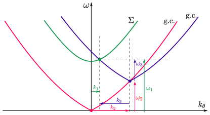
Figure 6: Graphical solution of the resonance conditions of Eq. (4) involving a sloshing wave decomposing into two gravity-capillary waves using the corresponding dispersion relations. One of the waves has to be counter-propagating to verify Eq. (4).

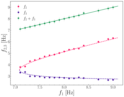
Figure 7: Measured values (dots) of the daughter frequencies $f_{2}$ (red) and $f_{3}$ (blue) for different mother frequencies $f_{1}$. The dashed lines are theoretical values obtained numerically through the resonance conditions of Eq. (4). Solid line of slope 1 corresponds to $f_{1}$ and green dots indicate the sum $f_{2}+f_{3}$.

Due to the periodicity of the system and its finite size, the dispersion relation of the torus is necessarily discrete [42]. If we denote by $\Delta_{\omega}\equiv\omega(k_{\theta}+1)-\omega(k_{\theta})$ the frequency gap between two adjacent discrete wavenumber $k_{\theta}$ and by $\Gamma_{\omega}$ the frequency nonlinear broadening of the dispersion relation, we can experimentally estimate whether discrete effects are to be taken into account ($\Gamma_{\omega}/\Delta_{\omega}\ll 1$) or if the system is in a kinetic regime ($\Gamma_{\omega}/\Delta_{\omega}\gg 1$) [46]. Indeed, we find approximately that $\Gamma_{\omega}/\Delta_{\omega}\in[3,6]$ in our experiment, hence we can consider the dispersion relation continuous.

The two daughter frequencies are now measured for different values of the mother frequency $f_{1}$ to confirm that the resonance conditions are well satisfied. Both the numerical solution of Eq. (4) (dashed lines), and the experimentally found values (dots) of $f_{1}$ and $f_{2}$ are in very good agreement as shown in Fig. 7. As we can see the frequencies satisfy the conditions extremely well, and not only confirm the frequency matching condition but also wavenumber conservation since this is implicitly included when solving the resonance conditions in Eq. (4). This confirms that the system is experiencing a resonant three-wave (two-branch) interaction. We note that below the cutoff frequency $\omega_{0}$ of the sloshing branch ($f_{0}<7.1$ Hz - see Figs. 2 and 5), no solution occurs in Fig. 7. Indeed, forcing below $f_{0}$ does not lead experimentally to the appearance of nonlinear resonant interactions.

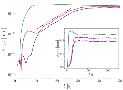
Figure 8: Semilog plot of amplitudes $A_{i}$ as a function of time of the mother wave (green, $f_{1}=7.4$ Hz), and the two daughter waves (in red and blue) measured using the Hilbert transform. We can observe that at around $12$ s the two daughters start growing exponentially as $e^{t/\tau}$ with $\tau=7$ s (dashed line). Inset: same in linear scale for the whole duration of the experiment, $T=240$ s. We can see how initially, as the daughter waves grow, the mother wave has to lose energy.

III.3 Wave amplitude growth

Three-wave interactions are usually described using amplitude equations. We now consider the amplitudes of each wave at frequency $f_{i}$, which are experimentally accessible through the use of the Hilbert transform of $\eta(t)$ [11]. This is done by first using a bandpass filter around the frequency of interest, onto which the Hilbert transform is then applied. This procedure then yields both the wave amplitude at frequency $f_{i}$ but also its phase $\varphi_{i}$.

We focus first on the displacement $\eta(t)$ forced at $f_{1}=7.4$ Hz from which we extract the three amplitudes. As we saw in Fig. 4 (middle), some typical time is needed for the transfer of energy from the mother wave $f_{1}$ into the daughters $f_{2}$ and $f_{3}$. The temporal evolutions of the amplitudes of all three waves are shown in Fig.  8. Once the mother wave is established, ($t<3$ s) it then increases rapidly up to a stationary out-of-equilibrium state ($t>10$ s). The growth is indeed balanced by dissipation when it begins pumping the daughter waves which grow exponentially, ($12<t<25$ s). Eventually, all three reach a stationary state ($t>35$ s). The exponential growth of the two daughter waves indicates that they undergo an instability. In addition, the mother wave reaches an initially higher amplitude which then decreases to the steady one, since it transfers energy to the two daughter waves through the instability. It is important to note that the three amplitudes are of the same order of magnitude, and the mother wave cannot be considered to be much stronger than the daughter waves as it is usual in three-wave resonant interactions [8, 11, 26].

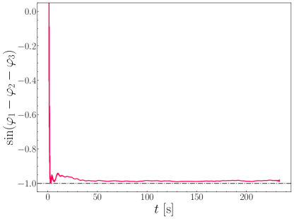
Figure 9: Temporal evolution of the sine of the total phase $\varphi=\varphi_{1}-\varphi_{2}-\varphi_{3}$ of the three waves obtained using the argument of the Hilbert transform. The total phase $\varphi$ is found to be locked to a value close to $-\pi/2$. Same forcing as in Fig. 8.

III.4 Phase locking

The phase of each wave reads $\varphi_{j}(\theta,t)=k_{\theta}\theta-\omega t+\phi_{j}$ and in general, it depends on time, $\phi_{j}$ being an initial arbitrary constant. Conversely, when Eq. (4) is satisfied, the interaction phase defined as $\Phi=\varphi_{1}-\varphi_{2}-\varphi_{3}$ remains constant (i.e., $\phi_{1}-\phi_{2}-\phi_{3}=\mathrm{const.}$), thus making the three waves phase-locked. Experimentally, $\varphi_{i}$ is measured by the argument of the Hilbert transform of $\eta(t)$ in the stationary regime.

To avoid possible phase jumps, we plot the sine of the total phase $\Phi$ in Fig. 9. Once the stationary regime is reached, the total phase remains constant over time. The three waves are thus phase-locked around $\Phi\simeq-\pi/2$ as expected theoretically for a three-wave resonant mechanism (see Sec. III.5).

III.5 Amplitude equations

We now consider the three-wave amplitude equations in the case of resonant interaction [47, 34] for a physical description of this instability

$$\dot{A}_{1}=iI_{23}A_{2}A_{3}{\rm\,,}$$ (5)

$$\dot{A}_{2}=iI_{13}A_{1}A_{3}^{*}{\rm\,,}$$ (6)

$$\dot{A}_{3}=iI_{12}A_{1}A_{2}^{*}{\rm\,,}$$ (7)

with $A_{i}$ the complex wave amplitude and $I_{i,i+1}$ are the unknown positive interaction coefficients. Note that the latter are known for gravity-capillary wave interaction involving no sloshing [48]. We will not approach the full problem of the above equations, which constitute an integrable system [49]. We instead focus only on the case where the pump-wave has a fixed amplitude $A_{1}$ (the so-called pump-wave approximation). Indeed, we saw experimentally that the stationary regime of the mother wave is established before the one of two daughter waves. For completeness, we include damping as well, leading to

$$\dot{A_{2}}=iI_{13}A_{1}A_{3}^{*}-\alpha_{2}A_{2}{\rm\,,}$$ (8)

$$\dot{A_{3}}=iI_{12}A_{1}A_{2}^{*}-\alpha_{3}A_{3}{\rm\,,}$$ (9)

with $\alpha_{j}$ the temporal damping rate of wave $j$. Inserting Eq. (8) into Eq. (9) leads to

$$\ddot{A_{3}}=I_{13}I_{12}A_{3}|A_{1}|^{2}-(\alpha_{2}+\alpha_{3})\dot{A}_{3}-\alpha_{2}\alpha_{3}A_{3}{\rm\,,}$$ (10)

which has a solution of the form

$$A_{3}=a_{+}e^{\sigma_{+}t}+a_{-}e^{\sigma_{-}t}{\rm\,,}$$ (11)

with $a_{\pm}$ depending on the initial conditions and the growth rate obeying

$$\sigma_{\pm}=-\frac{\alpha_{2}+\alpha_{3}}{2}\pm\sqrt{I_{12}I_{13}|A_{1}|^{2}+\frac{(\alpha_{2}-\alpha_{3})^{2}}{4}}{\rm\,.}$$ (12)

Thus an instability (i.e., $\sigma_{+}>0$) can be observed provided the mother amplitude overcomes a threshold due to dissipation. The daughter waves then grow exponentially, as observed experimentally. This means that if at time $t=0$, only wave $1$ has a finite amplitude, the other two waves, which are infinitesimal in magnitude, will be pumped up exponentially, and eventually be bounded by damping. The exact values of the interaction coefficients would follow from a weak nonlinear expansion of equations of motion, which for the case of the torus in this experimental geometry are so far unknown.

As for the phases of the waves, denoting $A_{j}=a_{j}e^{i\varphi_{j}}$ yields the equation for the temporal evolution of the total phase [47]

$$\dot{\Phi}=a_{1}a_{2}a_{3}\left(\frac{I_{23}}{a_{1}^{2}}-\frac{I_{13}}{a_{2}^{2}}-\frac{I_{12}}{a_{3}^{2}}\right)\cos\Phi=\beta\cos\Phi{\rm\,.}$$ (13)

If we consider that in the final stationary state all three amplitudes are constant, one finds a solution of the form

$$\Phi=2\arctan\left[\tanh\left(\frac{\beta(t_{0}+t)}{2}\right)\right]{\rm\,,}$$ (14)

which at large $t$ leads to $\varphi=\textup{sgn}(\beta)\pi/2$. Depending on the sign of $\beta$, i.e., the values of the interaction coefficients and amplitudes, the sign of the total phase will be differently determined, which we find experimentally to be $-\pi/2$. We find that the interaction phase $\Phi$ does not change with the frequency of the mother wave in the experiment.

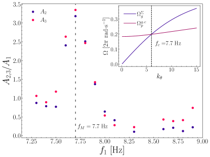
Figure 10: Normalized amplitudes of the two daughter waves for different frequencies of the mother wave $f_{1}$. We clearly observe a peak at around $f_{M}\approx 7.7$ Hz, where the daughter waves are three times larger than the mother wave in amplitude. Inset: Predicted group velocity of the sloshing mode (blue) and phase velocity of gravity-capillary mode (red), intersecting at $k_{c}=6$ corresponding to the peak frequency $f_{M}=7.7$ Hz.

III.6 Maximal energy transfer by velocity matching

We now turn to the dependence of the daughter amplitudes on the frequency $f_{1}$ of the mother wave. The daughter wave amplitudes normalized by the mother wave $A_{2,3}/A_{1}$ are shown as a function of $f_{1}$ in Fig. 10. The two daughter waves appear to follow the same relation and experience a maximal relative amplitude, making their amplitudes significantly larger than the mother wave. The plot is strongly reminiscent of the resonance curve of a driven harmonic oscillator. The peak of this curve, experimentally found to be at $f_{M}=7.7$ Hz, has to be located at a frequency that depends only on the system properties. We find it to be close to the frequency $\omega_{\Sigma}(k_{c})$ where $k_{c}=6$ is the wavenumber at which the group velocity, $\Omega^{\Sigma}_{g}=\textup{d}\omega_{\Sigma}/\textup{d}k_{\theta}$, of the sloshing branch and the phase velocity of the gravity-capillary, $\Omega^{\mathrm{gc}}_{p}=\omega_{\mathrm{gc}}/k_{\theta}$, intersect, numerically found to be $f_{c}\approx 7.7$ Hz, shown in the inset of Fig. 10.

The energy transfer is thus most efficient when a velocity matching occurs between the group velocity of the sloshing mode and the phase velocity of the gravity-capillary mode. Such an atypical velocity matching involving group and phase velocities differs from the usual phase-phase velocity matching [50], but has been considered theoretically for surface and internal waves [51, 52]. The energy transfer is thus found to be maximal when the carrier of a sloshing wavepacket has the same velocity as a gravity-capillary monochromatic wave for an identical wavenumber. Note that the efficiency of the wave interaction is thus related to the velocity matching, whereas the triadic interaction is the transfer mechanism.

Sloshing branches have previously been modeled, in the linear case, using systems of oscillators [53], while their nonlinear interaction remains more complicated. A model of the branch interaction would have to resemble the driven harmonic oscillator whose amplitude depends on $\omega_{c}^{2}-\omega_{3}^{2}$, similar to that found in [9], where $\omega_{c}=\omega_{\Sigma}(k_{c})$ is the frequency at which $\Omega_{p}^{\mathrm{gc}}=\Omega_{g}^{\Sigma}$.

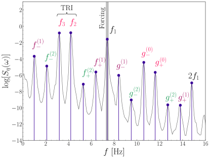
Figure 11: Power spectrum of a signal forced at $f_{1}=7.4$ Hz. The forcing is strong enough to excite additional couples besides the primary three-wave pairs, $f_{1}^{(1)}$ and $f_{2}^{(1)}$. The first two daughters, continue to generate firstly the subharmonic secondary waves of Eq. (15), which then go on to create tertiary waves through interactions with the mother wave at $f_{1}$.

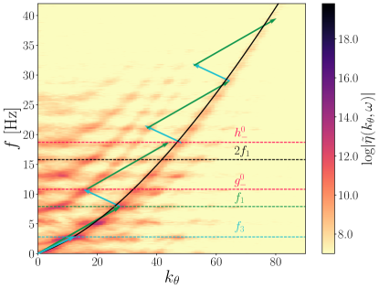
Figure 12: Fourier spectrum $\tilde{\eta}(k_{\theta},f)$ of the torus outer border displacement $\eta(\theta,t)$. Most of the energy is concentrated along the gravity-capillary branch. Quasiresonant interaction is observed following Eq. (17) and Eq. (18) with $\delta k_{\theta}=1.6$. Monochromatic forcing at $f_{1}=7.9$ Hz.

III.7 Subfrequency wave generation

As already noted at the bottom of Fig. 4, more than the expected three frequencies appear in the spectrum for high enough forcings. In order to better understand this, we apply a stronger monochromatic forcing leading to the power spectrum in Fig. 11. As shown above, the forcing frequency $f_{1}$, through the TRI, creates two daughters at $f_{2}$ and $f_{3}$. Under sufficiently strong forcing, these two daughters, through three-wave interactions create a second pair of frequencies which satisfies

$$\begin{split}f_{2}-f_{3}&=f_{-}^{(1)}{\rm\,,}\\ f_{-}^{(1)}+f_{+}^{(1)}&=f_{1}{\rm\,,}\end{split}$$ (15)

where $f_{\pm}^{(1)}$ is the first generation of secondary waves, the superscript indicating the generation order and the subscript sign indicates the relative value. The notation $+$ indicates the largest of the pair $f_{\pm}$ and vice-versa. The relationship between the frequencies, governed by Eq. (15), is well verified experimentally in Fig. 11. These grand-daughters can go on generating another generation $f^{(2)}_{\pm}$ in exactly the same way, which can then be repeated again and so on, thus populating the region with a high number of discrete peaks (see Fig. 11). This mechanism (analogous to that described for internal waves [19]) leads to a discrete type of energy cascade, where energy is transmitted into all the different possible daughter-wave generations. More generally, we have for the $n$th wave generation

$$\begin{split}f_{2}-f_{3}&=f_{-}^{(n)}{\rm\,,}\\ f_{-}^{(n)}+f_{+}^{(n)}&=f_{1}{\rm\,,}\end{split}$$ (16)

as also well observed in Fig. 11.

III.8 Upper-frequency wave generation

Let us now focus on the high-frequency part of the spectrum ($f_{1}<f<2f_{1}$) in Fig. 11. The corresponding discrete set of peaks is formed in a way similar to that of in Sec. III.7, but involving interaction with $f_{1}$. We find that these tertiary waves arise from the interaction of the daughter waves ($f_{2,3}$) or of the secondary waves ($f^{(n)}_{\pm}$) with the mother wave $f_{1}$. We find that they satisfy the following conditions:

$$\begin{split}f_{2,3}+f_{1}&=g^{(0)}_{\pm}{\rm\,,}\\ f^{(n)}_{\pm}+f_{1}&=g^{(n)}_{\pm}{\rm\,.}\end{split}$$ (17)

Note that the zeroth generation ($g^{0}_{\pm}$) is determined by the daughter waves $f_{2}$ and $f_{3}$, whereas the $n$th generation ($n>0$) involves the secondary waves. This relationship is verified in Fig. 11. Such interaction thus provides a way to populate the high-frequency content of the spectrum with discretely excited modes. The generation mechanism of Eq. (17) is further iterated, e.g., $g^{(0)}_{\pm}+f_{1}=h^{(0)}_{\pm}$, $g^{(n)}_{\pm}+f_{1}=h^{(n)}_{\pm}$, as observed experimentally (not shown in Fig. 11).

To determine whether tertiary waves lie on the dispersion relation and are also resonant in wavenumber we compute the experimental space-time Fourier spectrum $\tilde{\eta}(k_{\theta},f)$ of the torus outer border displacement as shown in Fig. 12. First, we can indeed observe that the excited tertiary waves lie on the dispersion relation. Interestingly, for a given tertiary wave, all branches present at that frequency are excited. But, looking more carefully and taking $g_{-}^{0}$ as an example, we find that

$$k_{\Sigma}\left(g_{-}^{0}\right) =k_{{\mathrm{gc}}}(f_{1})+k_{{\mathrm{gc}}}(f_{3})+\delta k_{\theta}{\rm\,,}$$ (18)

$$g_{-}^{0} =f_{1}+f_{3}{\rm\,,}$$ (19)

where $\delta k_{\theta}$ corresponds to the widening of the gravity-capillary dispersion branch due to nonlinearity. $\delta k_{\theta}$ is inferred from the standard deviation of a Gaussian fit around the peak of the Fourier spectrum at a fixed $f$. Equation (18) implies that a quasiresonant interaction occurs in wavenumber. We observed this in Fig. 12, since the frequencies have a perfect match, whereas the wavenumbers require broadening to fall on the dispersion relation.

III.9 Bicoherence

Finally, we experimentally quantify the three-wave interactions (i.e., $\nu_{1}+\nu_{2}=\nu_{3}$) by computing the normalized third-order correlation in frequency of the wave elevation called bicoherence [54]

$$B(\nu_{1},\nu_{2})=\frac{\left|\left\langle\tilde{\eta}^{*}(\nu_{1})\tilde{\eta}^{*}(\nu_{2})\tilde{\eta}(\nu_{1}+\nu_{2})\right\rangle\right|}{\sqrt{\langle|\tilde{\eta}(\nu_{1})\tilde{\eta}(\nu_{2})|^{2}\rangle\langle|\tilde{\eta}(\nu_{1}+\nu_{2})|^{2}\rangle}}{\rm\,,}$$ (20)

where $*$ denotes the complex conjugate. $\langle\cdot\rangle$ corresponds to an ensemble average over 101 temporal windows of the signal. The normalization is such that $B\in[0,1]$ where $0$ represents no correlation and $1$ a perfect correlation.

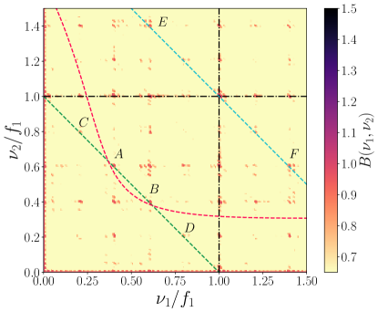
Figure 13: Bicoherence $B(\nu_{1},\nu_{2})$ of a wave elevation signal, recorded during $40$ min, at a given point. Forcing: sine wave with $f_{1}=7.5$ Hz. The mother wave is located at $(1,1)$, while all possible pairs whose sum is $1$ are on the green oblique dashed line of slope $-1$. The two daughter waves are located at the intersection of this line with the resonant manifold (dashed red line), solutions of Eq. (4), at points $A(f_{2},f_{3})$ and $B(f_{3},f_{2})$. Points $C$ and $D$ satisfy Eq. (15)b whereas points $E$ and $F$ follow Eq. (17)b.

The bicoherence for a monochromatic forcing at $7.5$ Hz is depicted in Fig. 13. We observe the primary mother wave at $(1,1)$. Note that $B(\nu_{1},\nu_{2})$ is symmetric about the $\nu_{2}=\nu_{1}$ diagonal. Moreover, the green dashed line shows all of the frequency pairs whose sum is $f_{1}$, but not all of them form resonant triads. The resonant triad $f_{1}=f_{2}+f_{3}$ is only found to occur at the points $A$ and $B$, which are the intersection points between the green dashed line and the red dashed line coming from solving the resonance conditions of Eq. (4). We can see that the daughters are located on the intersection of the resonant manifold with the frequency-sum line.

We can see that the plane is populated by other points, some of which are trivial (e.g., $f_{1},f_{1}$), as well as secondary and tertiary waves. According to Eq. (15)b, secondary waves will be located on the green dashed line since their sum yields $f_{1}$. The first generation $f^{(1)}_{\pm}$ is found at points $C$, and by symmetry, $D$.

Tertiary waves, however, can be seen to satisfy $g_{\pm}^{(n)}+f^{(n)}_{\mp}=2f_{1}$ according to Eq. (17)b and using Eq. (16)b. This is evidenced in Fig. 13 by points E and F, lying on the cyan dashed line which contains all points whose sum is equal to $2f_{1}$.

IV Conclusion

We have demonstrated the existence of nonlinear three-wave resonant interactions occurring between two different branches of the hydrodynamic wave dispersion relation, namely the gravity-capillary and sloshing modes. To the best of our knowledge, this three-wave two-branch interaction mechanism has never been reported experimentally in any wave system.

The system used is a torus of fluid for which the sloshing mode can easily be excited. When subjected to a weak monochromatic forcing, a triadic resonance instability is first observed with an exponential growth of the daughter waves and a phase locking of the three waves. The efficiency of this interaction is found to be maximum when the gravity-capillary phase velocity matches the group velocity of the sloshing mode. The interaction between waves belonging to these two branches can be considered as an analog of a forced harmonic oscillator. For stronger forcing, additional waves are generated by a cascade of three-wave interactions populating the high-frequency part of the wave spectrum. Since this mechanism authorizes three-wave interactions in a 1D system far from the gravity-capillary transition, it thus paves the way to reach a wave turbulence regime triggered by this atypical mechanism.

In the future, we plan to explore the role of the system periodicity on the wave interactions and on a possible wave turbulence regime, as previously shown for solitons [43]. Finally, such a three-wave two-branch interaction mechanism is probably not restricted to hydrodynamics and could be of primary interest in other fields involving several propagation modes, such as elastic plates [33], or optical waveguides [55].

- [1] V. E. Zakharov, V. S. L’vov, and G. Falkovich, Kolmogorov Spectra of Turbulence. I: Wave Turbulence (Springer, Berlin, Germany, 1992).
- [2] L. Stenflo, Resonant three-wave interactions in plasmas, Phys. Scr. T50, 15 (1994).
- [3] S. Hoijer and H. Wilhelmsson, Studies of nonlinear resonance conditions for three-wave interactions in a plasma, Plasma Phys. 12, 585 (1970).
- [4] J. A. Armstrong, N. Bloembergen, J. Ducuing, and P. S. Pershan, Interactions between light waves in a nonlinear dielectric, Phys. Rev. 127, 1918 (1962).
- [5] C. P. Connaughton, B. T. Nadiga, S. V. Nazarenko, and B. E. Quinn, Modulational instability of Rossby and drift waves and generation of zonal jets, J. Fluid Mech. 654, 207 (2010).
- [6] T. Guo, H. Kang, L. Wang, and Y. Zhao, Triad mode resonant interactions in suspended cables, Sci. China Phys., Mech. 59, 634501 (2016).
- [7] D. A. Kovriguine and A. I. Potapov, Nonlinear oscillations in a thin ring - i. three-wave resonant interactions, Acta Mech. 126, 189 (1998).
- [8] F. Haudin, A. Cazaubiel, L. Deike, T. Jamin, E. Falcon, and M. Berhanu, Experimental study of three-wave interactions among capillary-gravity surface waves, Phys. Rev. E 93, 043110 (2016).
- [9] A. Cazaubiel, F. Haudin, E. Falcon, and M. Berhanu, Forced three-wave interactions of capillary-gravity surface waves, Phys. Rev. Fluids 4, 074803 (2019).
- [10] L. Deike, M. Berhanu, and E. Falcon, Experimental observation of hydroelastic three-wave interactions, Phys. Rev. Fluids 2, 064803 (2017).
- [11] F. Bonnefoy, F. Haudin, G. Michel, B. Semin, T. Humbert, S. Aumaître, M. Berhanu, and E. Falcon, Observation of resonant interactions among surface gravity waves, J. Fluid Mech. 805, R3 (2016).
- [12] S. Liu, T. Waseda, and X. Zhang, Four-wave resonant interaction of surface gravity waves in finite water depth, Phys. Rev. Fluids 7, 114803 (2022).
- [13] G. Ricard and E. Falcon, Experimental quasi-1D capillary-wave turbulence, Europhys. Lett. 135, 64001 (2021).
- [14] A. Dyachenko, Y. Lvov, and V. Zakharov, Five-wave interaction on the surface of deep fluid, Physica D 87, 233 (1995).
- [15] Y. Lvov, Effective five-wave Hamiltonian for surface water waves, Phys. Lett. A 230, 38 (1997).
- [16] K. Hasselmann, A criterion for nonlinear wave stability, J. Fluid Mech. 30, 737 (1967).
- [17] B. Bourget, T. Dauxois, S. Joubaud, and P. Odier, Experimental study of parametric subharmonic instability for internal plane waves, J. Fluid Mech. 723, 1 (2013).
- [18] H. Scolan, E. Ermanyuk, and T. Dauxois, Nonlinear fate of internal wave attractors, Phys. Rev. Lett. 110, 234501 (2013).
- [19] C. Brouzet, E. V. Ermanyuk, S. Joubaud, I. Sibgatullin, and T. Dauxois, Energy cascade in internal-wave attractors, Europhys. Lett. 113, 44001 (2016).
- [20] E. Monsalve, M. Brunet, B. Gallet, and P.-P. Cortet, Quantitative experimental observation of weak inertial-wave turbulence, Phys. Rev. Lett. 125, 254502 (2020).
- [21] G. Bordes, F. Moisy, T. Dauxois, and P.-P. Cortet, Experimental evidence of a triadic resonance of plane inertial waves in a rotating fluid, Phys. Fluids 24, 014105 (2012).
- [22] G. Davis, T. Jamin, J. Deleuze, S. Joubaud, and T. Dauxois, Succession of resonances to achieve internal wave turbulence, Phys. Rev. Lett. 124, 204502 (2020).
- [23] C. Brouzet, E. Ermanyuk, S. Joubaud, G. Pillet, and T. Dauxois, Internal wave attractors: different scenarios of instability, J. Fluid Mech. 811, 544 (2017).
- [24] C. Savaro, A. Campagne, M. C. Linares, P. Augier, J. Sommeria, T. Valran, S. Viboud, and N. Mordant, Generation of weakly nonlinear turbulence of internal gravity waves in the Coriolis facility, Phys. Rev. Fluids 5, 073801 (2020).
- [25] Y. Pan, B. K. Arbic, A. D. Nelson, D. Menemenlis, W. R. Peltier, W. Xu, and Y. Li, Numerical Investigation of Mechanisms Underlying Oceanic Internal Gravity Wave Power-Law Spectra, J. Phys. Oceanogr. 50, 2713 (2020).
- [26] A. D. D. Craik and J. A. Adam, Evolution in space and time of resonant wave triads. i. the “pump-wave approximation”, Proc. R. Soc. Lond. 363, 243 (1978).
- [27] J. F. Drake, P. K. Kaw, Y. C. Lee, G. Schmid, C. S. Liu, and M. N. Rosenbluth, Parametric instabilities of electromagnetic waves in plasmas, Phys. Fluids 17, 778 (1974).
- [28] J. A. MacKinnon, M. H. Alford, O. Sun, R. Pinkel, Z. Zhao, and J. Klymak, Parametric subharmonic instability of the internal tide at 29on, J. Phys. Oceanogr. 43, 17 (2013).
- [29] H. Lamb, Hydrodynamics, (Cambridge University Press, Cambridge, UK, 1932).
- [30] E. Falcon, C. Laroche, and S. Fauve, Observation of gravity-capillary wave turbulence, Phys. Rev. Lett. 98, 094503 (2007).
- [31] E. Falcon and N. Mordant, Experiments in Surface Gravity-Capillary Wave Turbulence, Annu. Rev. Fluid Mech. 54, 1 (2022).
- [32] R. A. Ibrahim, Recent Advances in Physics of Fluid Parametric Sloshing and Related Problems, J. Fluids Eng. 137, 09 (2015).
- [33] J. Laurent, D. Royer, and C. Prada, In-plane backward and zero group velocity guided modes in rigid and soft strips, J. Acoust. Soc. Am. 147, 1302 (2020).
- [34] A. Marchenko, Resonance interactions of waves in an ice channel, J. Appl. Math. Mech. 61, 931 (1997).
- [35] K. Khusnutdinova and D. Pelinovsky, On the exchange of energy in coupled Klein-Gordon equations, Wave Motion 38, 1 (2003).
- [36] I. Akhatov, V. Baikov, and K. Khusnutdinova, Non-linear dynamics of coupled chains of particles, J. Appl. Math. Mech. 59, 353 (1995).
- [37] A. Pezzi, G. Deng, Y. Lvov, M. Lorenzo, and M. Onorato, Three-wave resonant interactions in the diatomic chain with cubic anharmonic potential: theory and simulations, arXiv:2103.08336 [cond-mat.stat-mech]
- [38] E. M. Tejero, C. Crabtree, D. D. Blackwell, W. E. Amatucci, G. Ganguli, and L. Rudakov, Experimental characterization of nonlinear processes of whistler branch waves, Phys. Plasmas 23, 055707 (2016).
- [39] F. Dias, P. Guyenne, and V. Zakharov, Kolmogorov spectra of weak turbulence in media with two types of interacting waves, Phys. Lett. A 291, 139 (2001).
- [40] J. Zaleski, P. Zaleski, and Y. V. Lvov, Excitation of interfacial waves via surface–interfacial wave interactions, J. Fluid Mech. 887, A14 (2020).
- [41] B. Issenmann, C. Laroche, and E. Falcon, Wave turbulence in a two-layer fluid: Coupling between free surface and interface waves, Europhys. Lett. 116, 64005 (2016).
- [42] F. Novkoski, E. Falcon, and C.-T. Pham, Experimental Dispersion Relation of Surface Waves Along a Torus of Fluid, Phys. Rev. Lett. 127, 144504 (2021).
- [43] F. Novkoski, C.-T. Pham, and E. Falcon, Experimental observation of periodic Korteweg-de Vries solitons along a torus of fluid, Europhys. Lett. 139, 53003 (2022).
- [44] G. Le Doudic, S. Perrard, and C.-T. Pham, Surface waves along liquid cylinders. Part 2. varicose, sinuous, sloshing and nonlinear waves, J. Fluid Mech. 923, A13 (2021).
- [45] S. Nazarenko, Wave Turbulence (Springer, Berlin, 2011).
- [46] V. S. L’vov and S. Nazarenko, Discrete and mesoscopic regimes of finite-size wave turbulence, Phys. Rev. E 82, 056322 (2010).
- [47] A. D. D. Craik, Wave Interactions and Fluid Flows, (Cambridge University Press, Cambridge, UK, 1986).
- [48] W. F. Simmons and M. J. Lighthill, A variational method for weak resonant wave interactions, Proc. R. Soc. Lond. A 309, 551 (1969).
- [49] D. J. Kaup, The three-wave interaction – A nondispersive phenomenon, Stud. Appl. Math. 55, 9 (1976).
- [50] A. V. Fedorov, W. K. Melville, and A. Rozenberg, An experimental and numerical study of parasitic capillary waves, Phys. Fluids 10, 1315 (1998).
- [51] T. Kawahara, N. Sugimoto, and T. Kakutani, Nonlinear interaction between short and long capillary-gravity waves, J. Phys. Soc. Japan 39, 1379 (1975).
- [52] T. M. A. Taklo and W. Choi, Group resonant interactions between surface and internal gravity waves in a two-layer system, J. Fluid Mech. 892, A14 (2020).
- [53] R. A. Ibrahim, V. N. Pilipchuk, and T. Ikeda, Recent Advances in Liquid Sloshing Dynamics, Appl. Mech. Rev. 54, 133 (2001).
- [54] V. Kravtchenko-Berejnoi, F. Lefeuvre, V. Krasnossel’skikh, and D. Lagoutte, On the use of tricoherent analysis to detect nonlinear wave-wave interactions, Signal Process. 42, 291 (1995).
- [55] A. Ghatak and K. Thyagarajanm, An Introduction to Fiber Optics, (Cambridge University Press, Cambridge, UK, 1998).