Algebroid Solutions of the Degenerate Third Painlevé Equation for Vanishing Formal Monodromy Parameter

Abstract

Various properties of algebroid solutions of the degenerate third Painlevé equation,

$$u^{\prime\prime}(\tau)\!=\!\frac{(u^{\prime}(\tau))^{2}}{u(\tau)}\!-\!\frac{u^{\prime}(\tau)}{\tau}\!+\!\frac{1}{\tau}\!\left(-8\varepsilon(u(\tau))^{2}\!+\!2ab\right)\!+\!\frac{b^{2}}{u(\tau)},\qquad\varepsilon=\pm 1,\quad\varepsilon b>0,$$

for the monodromy parameter $a=0$ are studied. The paper contains connection results for asymptotics as $\tau\to+0$ and as $\tau\to+\infty$ for $a\in\mathbb{C}$. Using these results, the simplest algebroid solution with asymptotics $u(\tau)\to c\tau^{1/3}$ as $\tau\to 0$, where $c\in\mathbb{C}\setminus\{0\}$, together with its associated integral $\smallint_{0}^{\tau}{(u(t))^{-1}\,\mathrm{d}t}$, are considered in detail, and their basic asymptotic behaviours are visualized.

2020 Mathematics Subject Classification. 33E17, 34M30, 34M35, 34M40, 34M55, 34M56,

20F55

Abbreviated Title. Algebroid Solutions of the Degenerate Third Painlevé Equation

Key Words. Algebroid function, asymptotics, Coxeter group, monodromy manifold, Painlevé

equation

1 Introduction

We consider the degenerate third Painlevé equation [25, 26] in the form

$$u^{\prime\prime}(\tau)\!=\!\frac{(u^{\prime}(\tau))^{2}}{u(\tau)}\!-\!\frac{u^{\prime}(\tau)}{\tau}\!+\!\frac{1}{\tau}\!\left(-8\varepsilon(u(\tau))^{2}\!+\!2ab\right)\!+\!\frac{b^{2}}{u(\tau)},$$ (1.1)

where the prime denotes differentiation with respect to $\tau$, $\varepsilon=\pm 1$, and $b\in\mathbb{R}\setminus\{0\}$ and $a\in\mathbb{C}$ are parameters. Equation (1.1) is also refered as the third Painlevé equation of $D_{7}$ type [32].

Algebroid solutions of equation (1.1) can be viewed as meromorphic solutions of the Painlevé-type equations that are equivalent, in the sense of Ince’s classification [23], to equation (1.1); therefore, it is natural to extend some results and ideas developed by one of the authors of this work in [28] for the study of the meromorphic solutions of (1.1) to this wider class of solutions. The algebroid solutions represent an interesting class of solutions from the point of view of their asymptotics, because their large-$\tau$ asymptotic behaviour can be explicitly expressed in terms of the initial values of the associated meromorphic functions. Recall that, in a generic situation, such explicit formulae are not obtainable for any Painlevé equation. At the same time, however, the behaviour of the algebroid solutions at the point at infinity resembles the behaviour of generic solutions; so, we take this opportunity to “visualize the asymptotics”, namely, we consider several examples of initial values for the simplest algebroid solution and compare the graphs of the numerical solutions with their asymptotics. This comparison elucidates many interesting features of the numeric-asymptotic correspondence. In view of the present asymptotic study, we’ve included updated and reformulated connection results obtained in [26, 27] for asymptotics of solutions of equation (1.1) for generic $a\in\mathbb{C}$ in Appendices B and C. A detailed description of the contents of this paper is given below, after a brief account of the literature.

We now mention some works that are related to the topic of our study. Gromak [17] proved that the general third Painlevé equation has algebraic solutions iff it reduces (with, perhaps, the help of the transformation $u(\tau)\to 1/u(\tau)$) to the degenerate case (1.1) with $\mathrm{i}a=n\in\mathbb{Z}$: for each $n$, equation (1.1) has exactly three solutions of the form $R(x)$, where $R$ is a rational function and $(2\varepsilon x)^{3}=b^{2}\tau$. From the functional point of view, we have one multi-valued function, and the three solutions are obtained via a cyclic permutation of the sheets of the Riemann surface $(2\varepsilon x)^{3}=b^{2}\tau$. The function $R(x)$ can be constructed via a successive application of the Bäcklund transformations to the three different solutions $u(\tau)=\tfrac{\varepsilon}{2}\sqrt[3]{b^{2}\tau}$ of (1.1) for the simplest case $a=0$. Recently, Buckingham and Miller [7] studied a double-scaling limit of the algebraic solution as $n\to\infty$ and $\tau/n^{3/2}=\mathcal{O}(1)$.

Among other asymptotic results for equation (1.1) that concern its general solutions, we mention the recent paper by Shimomura [36] on the elliptic asymptotic representation of the general solution of (1.1) in terms of the Weierstrass $\wp$-function in cheese-like strip domains along generic directions in $\mathbb{C}\setminus\left(\mathbb{R}\cup\mathrm{i}\mathbb{R}\right)$. Another interesting paper by Gamayun, Iorgov, and Lisovyy [16] gives, in particular, a derivation of the asymptotic expansions via a proper double-scaling limit from the sixth Painlevé equation to the degenerate third Painlevé equation, with emphasis placed on the combinatorial properties of the coefficients of the asymptotic expansions.

In the last decade, an ever-increasing number of papers dedicated to the application of the degenerate third Painlevé equation and its generalizations, e.g., the cylindrical reduction of the Toda system, to some models in applied and theoretical physics and in geometry have appeared; see, for example, [3, 8, 9, 11, 12, 18, 19, 20, 21, 22, 39, 40, 41]. The majority of these works refer to, or report, some novel results in the asymptotic description of some special solutions appearing in particular applications. In this paper, we can not, nor do we attempt to, give an overview of these works, as such a presentation would lead us too far astray from our goals. As a matter of fact, it would be of considerable interest to prepare an account of these works in the form of a review article dedicated to the multifarious manifestations of the degenerate third Painlevé equation (1.1). Hereafter, we discuss only those works that are of primary relevance for our current research.

The main illustrative object of study in this article is the holomorphic at $r=0$ function $H(r)$ which solves the ordinary differential equation (ODE)

$$H^{\prime\prime}(r)\!=\!\frac{(H^{\prime}(r))^{2}}{H(r)}\!-\!\frac{H^{\prime}(r)}{r}\!+\!\frac{1}{r}\!\left((H(r))^{2}\!-\!\frac{1}{H(r)}\right),$$ (1.2)

where the prime denotes differentiation with respect to $r$. This function, in the real case $H(r)\in\mathbb{R}$ for $r\in\mathbb{R}$, was introduced by Bobenko and Eitner in [4] as the function defining the Blaschke metrics of the two-dimensional regular indefinite affine sphere in $\mathbb{R}^{3}$ with two affine straight lines. They proved, in particular, that, for this special class of the affine spheres, the function $H(r)$ is a similarity solution of the general Tzitzéica equation describing regular indefinite affine spheres in $\mathbb{R}^{3}$. The authors of [4] formulated a special Goursat boundary-value problem for the Tzitzéica equation: the solution of this problem is a similarity function which solves equation (1.2). Exploiting the unique solvability of the Goursat problem for second-order hyperbolic partial differential equations, Bobenko and Eitner proved the existence and the uniqueness of the smooth at $r=0$ real solution $H(r)$ of equation (1.2). Assuming, then, the existence of the smooth solution $H(r)$, they deduced from equation (1.2) that $H^{\prime\prime}(r)$ is also smooth, and, substituting the expansion

$$H(r)\underset{r\to 0}{=}H(0)+H^{\prime}(0)r+\mathcal{O}(r^{2}),$$ (1.3)

where $\mathcal{O}(r^{2})$ is a smooth function, into equation (1.2), proved that

$$H^{\prime}(0)=(H(0))^{2}-\frac{1}{H(0)}.$$ (1.4)

Bobenko and Eitner also showed that the Painlevé property of this equation allows one to make several useful, for the geometry of the affine sphere, conclusions about the qualitative behaviour of this solution; for example, if $H(0)>0$, then the solution has neither poles nor zeros on the negative-$r$ semi-axis, and, for $H(0)<0$, the smooth solution is growing monotonically from some—largest—pole on the negative-$r$ semi-axis to the first zero on the positive-$r$ semi-axis.

We now commence with the detailed discussion of the contents of this work.

Section 2 consists of two subsections. In Subsection 2.1, we prove that, for $H(0)\in\mathbb{C}\setminus\{0\}$, there exists a unique solution of equation (1.2) which is holomorphic at $r=0$: we use the straightforward method that is based on the proof of the convergence of a formal power series. This choice for the method of the proof is adopted because, in the following Subsection 2.2 and in Section 6, we use the recurrence relation that is analysed in Subsection 2.1. The main goal that we pursue in Subsection 2.2 is to study the coefficients of the Taylor-series expansion of $H(r)$ introduced in Subsection 2.1. Actually, our goal in this respect is two-fold: (i) to formulate some number-theoretic properties of these coefficients; and (ii) to give an effective tool for their calculation. After some preliminary results and experimentation with Maple, we were able to formulate a conjecture regarding the content of the polynomials in $a_{0}:=-H(0)$ defining the Taylor-series coefficients. A substantial part of Subsection 2.2 is devoted to the technique of generating functions for the calculation of the coefficients. This technique was suggested in [28] for the study of the Taylor coefficients of holomorphic solutions of equation (1.1) in the case where these coefficients are rational functions of the parameter $a\in\mathbb{C}\setminus\{0\}$. Equation (1.2) is related (see the discussion below) to equation (1.1), but with $a=0$, and our coefficients are functions of the parameter $H(0)$. Nevertheless, we show that the technique of generating functions is also applicable in this situation; moreover, in Appendix A, we present a stratagem that actually helps in the situation where straightforward calculations lead to cumbersome formulae.

Via the change of variables

$$y(t)\!=\!t^{1/3}H(r),\qquad r=\left(\frac{3}{4}\right)^{2}t^{4/3},$$ (1.5)

one shows that equation (1.2) transforms into the canonical form of the third Painlevé equation [23] with the coefficients $(1,0,0,-1)$,

$$y^{\prime\prime}(t)\!=\!\frac{(y^{\prime}(t))^{2}}{y(t)}\!-\!\dfrac{y^{\prime}(t)}{t}\!+\!\frac{(y(t))^{2}}{t}\!-\!\dfrac{1}{y(t)},$$ (1.6)

where the prime denotes differentiation with respect to $t$. Equation  (1.1) can also be identified as a special case of the canonical form of the third Painlevé equation with the following set of coefficients, $(-8\varepsilon,2ab,0,b^{2})$. One can, of course, identify equations (1.1) and (1.6) by setting $\varepsilon=-1/8$, $b=\pm\mathrm{i}$, and $a=0$; however, since we are planning on using the asymptotic results obtained in [26, 27], where it is assumed that $\varepsilon=\pm 1$ and $\varepsilon b>0$, we identify these equations by choosing, for the coefficients in equation (1.1), the values

$$\varepsilon\!=\!b\!=\!+1\qquad\text{and}\qquad a=0,$$ (1.7)

and making the following change of variables

$$\tau=2^{-3/2}\mathrm{e}^{3\pi\mathrm{i}/4}t\qquad\text{and}\qquad u(\tau)=-2^{-3/2}\mathrm{e}^{-3\pi\mathrm{i}/4}y(t).$$ (1.8)

For future reference, we rewrite the expansion (1.3) in terms of the functions $y(t)$ and $u(\tau)$; the expansion for $y(t)$ follows immediately from equations (1.3) and (1.5):

$$y(t)\underset{t\to 0}{=}t^{1/3}\!\left(H(0)+H^{\prime}(0)\!\left(3/4\right)^{2}t^{4/3}+\mathcal{O}\big{(}t^{8/3}\big{)}\right),$$ (1.9)

where the branches of $t^{1/3}$ and $t^{4/3}$ are defined to be positive for $t>0$. Now, equations (1.8) imply that

$$u(\tau)\underset{\tau\to+0}{=}\frac{1}{2}\tau^{1/3}\!\left(H(0)-H^{\prime}(0)(3/2)^{2}\tau^{4/3}+\mathcal{O}(\tau^{8/3})\right),$$ (1.10)

where the branches of $\tau^{1/3}$ and $\tau^{4/3}$ are defined analogously as for the powers of $t$ above, and the coefficient values (1.7) are assumed.

Section 3 begins with the general description of the algebroid solutions of equation (1.6). This consideration is based on the fact that equation (1.6) possesses the Painlevé property, and its solutons have only one branching point at the origin $t=0$; therefore, a solution is algebroid when the exponent defining its behaviour at the origin ($\tau=t=r=0$) is a rational number; moreover, there are no logarithmic terms in the complete asymptotic expansion as $t\to 0$ of this solution. After that, we define two particular series (infinite sequences) of algebroid solutions and show how to match the classical definition of the algebroid function (see, for example, [38]) as the solution of an algebraic equation with meromorphic coefficients. This approach is based on the study of the expansion of the solution as $t\to 0$. We derive a structure for the coefficients of this expansion as functions of the initial value $a_{0}$. This analysis is similar to the corresponding part of Subsection 2.2 for the study of the function $H(r)$; however, the combinatorics of the coefficients proves to be more interesting. We then deviate from the course of study of Subsection 2.2, and, instead of using generating functions for the coefficients, define, for each algebroid solution, with the help of its small-$t$ expansion, a set of meromorphic functions that are holomorphic at the origin. In terms of these meromorphic functions, we present an explicit construction for the algebraic equations of the algebroid solutions of the aforementioned series. This construction leads to the study of some interesting functional determinants. Finally, we derive systems of second-order differential equations which allow one to determine the meromorphic functions used for the construction of the algebraic equations mentioned above as the unique solutions of these systems that are holomorphic at the origin. We expect that the methodology expounded in Section 3 will work for the case of generic algebroid solutions of equation (1.1); technically, however, the explicit construction may prove to be unwieldy.

In Section 4, we return to the study of the function $H(r)$. We recall the definition of the monodromy manifold defined in our work [26] corresponding to the function $u(\tau)$ that solves (1.1) for the coefficient values (1.7). This manifold uniquely describes the pair of functions $u(\tau)$ and $\mathrm{e}^{\mathrm{i}\varphi(\tau)}$, where the function $\varphi(\tau)$ is an indefinite integral, that is, $\varphi^{\prime}(\tau)=2a/\tau+b/u(\tau)$. We see that the function $v(\tau):=\mathrm{e}^{\mathrm{i}\varphi(\tau)}$ depends on an additional multiplicative constant of integration compared to the function $u(\tau)$; moreover, as long as the function $v(\tau)$ is known, the function $u(\tau)$ can be readily obtained via differentiation. One can actually parametrize our system of isomonodromy deformations [26] in terms of the function $v(\tau)$ which solves, in its own right, a third-order Painlevé equation that can be derived from equation (1.1) via the substitution $u(\tau)=-b\left(2a/\tau+\mathrm{i}v^{\prime}(\tau)/v(\tau)\right)^{-1}$. Our goal, however, is to compare the asymptotic results of the papers [25] and [26]. Towards this end, we eliminate the multiplicative constant from the monodromy data of the monodromy manifold of [26] to arrive at the so-called contracted monodromy manifold, and show that the contracted manifold is equivalent to the monodromy manifold considered in the paper [25]. The main purpose of Section 4 is to explain how one can use the results of [26] in order to calculate the monodromy data corresponding to the solution (1.10) associated with $H(r)$ in terms of the initial value $H(0)$. For the reader’s convenience, some basic results from [26] that are necessary for understanding the material of this section are formulated in Appendix B. These results concern the asymptotic behaviour as $\tau\to 0$ of the function $u(\tau)$ and of its indefinite integral, $\varphi(\tau)$, related to equation (1.1) for generic parameter $a\in\mathbb{C}$, with $|\mathrm{Im}\,a|<1$. As discussed above, the function $\varphi(\tau)$ has a closely-knit relationship to the system of isomonodromy deformations studied in [26, 27], so that it is very helpful for the study of asymptotics of some definite integrals related to $u(\tau)$. Compared to [26], we have, in Appendix B, simplified the notation and some formulae, and have presented explicit asymptotics for the function $\varphi(\tau)$. It is our expectation that the detailed derivation presented in Section 4, in conjunction with the improved presentation for the asymptotic results given in Appendix B, will be of benefit to those readers for whom the derivation of analogous parametrizations for other types of solutions of (1.1) is required.

In Section 5, we give a group-theoretical characterization of the algebroid solutions of (1.1) for $a=0$. The contracted monodromy manifold “enumerating” the solutions of (1.1) for generic values of $a$ is a cubic surface in $\mathbb{C}^{3}$. The projectivization of this surface is a singular cubic surface in $\mathbb{CP}^{3}$ with a singularity of type $A_{3}$. With the help of a rational parametrization for this cubic surface, we derive its group of automorphisms, $G$. A formula for one of the generators of this group is not properly defined, thus we consider its regularization: this regularization is obtained for the restriction of the group $G$, denoted as $G(s)$, where $s$ is a Stokes multiplier, acting on a disjoint sum of two conics. These disjoint sums of two conics do not intersect for different values of $s$, so that continuing the action of $G(s)$ as the identity transformation on the complement of the contracted monodromy manifold to the conics on which $G(s)$ is acting non-trivially, we can present $G$ as an infinite direct sum of groups $G(s)$ with $s\in\mathbb{C}\setminus\{-1,3\}$. The group $G(s)$ is isomorphic to a Coxeter group of the type

$$\bullet\underset{4}{\tfrac{\phantom{xxxx}}{\phantom{xxxx}}}\bullet\underset{m}{\tfrac{\phantom{xxxx}}{\phantom{xxxx}}}\bullet$$

which has a normal subgroup isomorphic to the dihedral group $Dih_{m}$, $m\in\mathbb{N}\cup\{\infty\}$. The solution is algebroid iff the corresponding monodromy data belongs to the conics where $m$ is finite. This condition is equivalent to the statement that the corresponding Stokes multiplier $s$ is a real algebraic number that solves one of the polynomial equations $q_{m}(s)$, $m\in\mathbb{N}$, defined recursively in Section 5 with the help of the Chebyshev polynomials. The polynomials $q_{m}(s)$ are known in the mathematical literature as representing the “trigonometric” algebraic numbers; in particular, their Galois group is solvable, so that their roots which coincide with the Stokes multipliers of the algebroid solutions can be presented in terms of radicals.

Section 6 is devoted to the visualization of the large-$r$ asymptotics on the negative-$r$ semi-axis. In this section, we compare the numerical plots of the functions $H(r)$ and $I(r):=\smallint_{r}^{0}\tfrac{1}{\sqrt{-r}H(r)}\,\mathrm{d}r=(\varphi(\tau)-\varphi(0))\left.\right|_{\tau^{2/3}=\frac{2}{3}\sqrt{-r}}$ with the plots of their asymptotics, where the function $\varphi(\tau)$ is addressed above. For the convenience of the reader, we present a summary of our previous results [26, 27] on the small- and large-$\tau$ asymptotics for solutions of equation (1.1) for generic $a\in\mathbb{C}$ in Appendices B and C, respectively; furthermore, in these appendices, the reader will also find several new results for asymptotics of the function $\varphi(\tau)$. In our previous papers [27, 28, 29], we found and corrected some mistakes in [26]; therefore, we have amalgamated the corrected results in Appendices B and C. In addition, in these appendices, we improve the notation and simplify some of the formulae: all these changes are indicated therein.

By the locution “visualization of asymptotics” we mean the visual comparison of the plots of the numerical solutions with their asymptotics. The primary goal of this comparison is three-fold: (i) for different initial values $H(0)$, to observe the behaviour of the functions $H(r)$ and $I(r)$ at “finite” distances; (ii) to verify the correctness of the asymptotic formulae; and (iii) to understand at what rate these functions achieve their asymptotic behaviour. These goals are fundamental from the point of view of applications of these functions; however, it is by no means a trivial matter to put these concepts on rigorous mathematical footing.

Section 6 consists of six examples that were deliberately chosen in order to exhibit the dependence of the functions $H(r)$ and $I(r)$ on the initial value $H(0)$ on the negative-$r$ semi-axis, together with the features of their asymptotic approximations. These examples do not represent the complete list of known solutions: the solutions that are not mentioned here represent some special classes of solutions (in our case, solutions that depend on one real parameter) with some specific asymptotic behaviours; for example, solutions which are singular on the negative-$r$ semi-axis, or so-called truncated solutions [42].

There is an ancient proverb which states: “One look is worth a thousand words in a book”. In the context of our studies, it can be rephrased as the locution “visualization of asymptotics”. A “present-day look”, however, is not possible without the help of computer simulations, where the presentation of the results undergo a correction by the corresponding computer programs; thus, it is important to discuss some features of this correction. These features meddle with fact that equation (1.2) has a singularity at $r=0$, where the initial data is specified.

At first glance, everything appears to be simple: if one observes that the plots of a function and its asymptotics approach one another on some segment of reasonable length, then, one concludes that the asymptotics is correct…, or, most likely correct… A subtle point here, of course, is the notion of “reasonable length”, which is not that apparent. Since we are dealing with asymptotics, we have to verify them over relatively large distances, because, in certain situations, even though the numerical solution and its proposed asymptotics are close to one another over short distances, they may diverge over longer ones. This may occur, for example, if there is a minor mistake in the asymptotic formula: the behaviour of the solution has not yet stabilized and, at this stage, is partially compensated by a mistake, and some residual discrepancies between the plots can be explained by the fact that the asymptotics is not supposed to coincide exactly with the solution. In order to exclude the possibility of a mistake in the asymptotics, we have to increase the length of the interval of comparison. Doing so, however, may compromise the accuracy of the numerical solution, so that the asymptotics is correct, but the discrepancy between the two starts to grow. Both of these problems can be rectified, but as a result, one will have to compare the plots over relatively large intervals. Then, in order to fit into a standard page, the plots are appropriately scaled by a computer programme. As a result, some of the features of the plots may be lost, as, say, in our case, where in some of the figures presented in Section 6 (see, also, Figs. 1 and 2 below) the reader will see sharp peaks and icicles, even though all functions are, de facto, smooth, and, at their extremal points, the derivatives vanish, although “a look” shows that they are close to infinity. Another problem related to the scaling is the length of the first two peaks/icicles, which are the narrowest ones. The plot is built on the basis of a finite number of points of which very few land inside the narrow peaks/icicles. Actually, when the number of plot points are not sufficient, these peaks/icicles resemble a fence constructed from sticks of random lengths. Looking at such a plot, one can conclude that this situation occurs because the poles near the negative-$r$ semi-axis are located at random distances, which, however, is not the case! Of course, the behaviour of solutions at distances relatively close to the origin is not a particularly important problem from the point of view of asymptotics, because we want to see that everything is correct over distances longer than that of the location of the first two peaks/icicles; nevertheless, in many cases, the asymptotics resembles the behaviour of the numerical solutions even over these very small distances, which is related with the problem of how quickly the solutions attain their asymptotic behaviour; therefore, it is intriguing to observe the discrepancy between the corresponding plots even over such small distances. The true length of the first peaks/icicles can be determined by considering close-up pictures of these peaks/icicles, and in the most complicated cases by making numerical calculations with smaller step sizes. Then, one varies the number of points that are calculated for the generation of the plots in order to find a better correspondence for the lengths of the peaks/icicles. For the examples presented in Section 6, the discrepancy between the lengths of the first two peaks/icicles on both the scaled and close-up figures is about $5$ to $6$ percent, or less, whereas for the subsequent peaks/icicles this difference is not observable. We present such close-up pictures in some of the examples so that the reader can compare the real lengths of the peaks/icicles with the ones on the scaled figures. Such close-up pictures also show the reader the quality of the approximations of the numerical solutions by their large-$r$ asymptotics even over small distances: on the non-close-up figures, such approximations look better as a result of scaling.

One may ask: whence a notion of approximating a function at finite or even small distances by its large-$r$ asymptotics emanate? Well, “finite” and “small” are not well-defined notions; after all, on the practical level, if one wants to compare a function to its asymptotics, then one has to start this comparison from some “finite” value of the argument! Recalling the aforementioned proverb, the reader may ask: where does one have to cast “a look” to be sure that the asymptotics correctly approximates the function? Another point is that all mathematical models of practical value are applicable in some bounded domains (times, distances, etc.); therefore, it is imperative to know whether or not our asymptotics are actually applicable in, or far away from, the domains of interest.

The gist of the discussion in the previous paragraph can be visualized with the help of Figs. 1 and 2 below.

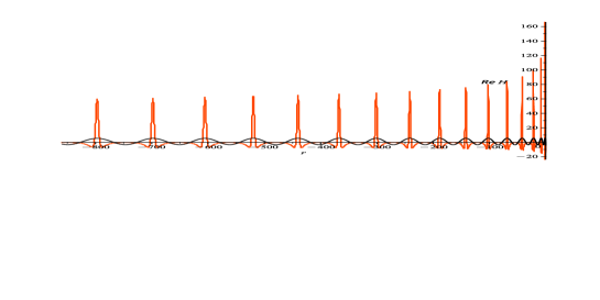
Figure 1: The red and black plots are, respectively, the real parts of the numeric and large-$r$ asymptotic (cf. equation (6.1)) values of the function $H(r)$ for $r\leqslant-0.1$ corresponding to the initial value $H(0)=-0.2+\mathrm{i}0.045$ (see Subsection 6.6).

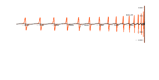
Figure 2: The red and black plots are, respectively, the imaginary parts of the numeric and large-$r$ asymptotic (cf. equation (6.1)) values of the function $H(r)$ for $r\leqslant-0.1$ corresponding to the initial value $H(0)=-0.2+\mathrm{i}0.045$ (see Subsection 6.6).

In Figs. 1 and 2, the red plots are the real and imaginary parts, respectively, of the function $H(r)$ considered in Example 6 of Section 6. The black plots in these figures are the corresponding leading terms of asymptotics. “A look” seems to suggest that something is wrong: (i) perhaps it’s the asymptotics; (ii) perhaps it’s the distance whence the asymptotics start to work; or (iii) perhaps it’s the absence of the correction terms? Our claim is the following: (i) the asymptotics are, in fact, correct; (ii) the proper distances over which these facts can be visualized can not be attained numerically; and (iii) a finite number of correction terms will not help to visualize that the asymptotics are correct, even though they may be beneficial for improving the correspondence of the plots on larger distances relative to the origin. We now justify our claims. How do we know that the asymptotics are correct? We have, in fact, two asymptotic formulae with overlapping domains of applicability, one of which obtained in [26], the other in [27]. The formula taken from [26] is visualized in Figs. 1 and 2, where as the formula taken from 2 is visualized in Figs. 33 and 35 of Subsec 6.6: this visualization shows that the latter formulae approximate the numerical solution with a very high degree of accuracy for $r\leqslant-0.1$. This formula from [27] can be further simplified for very large values of $|r|$, so that we can find, so to say, the “asymptotics of asymptotics”, and thus obtain a simplified asymptotic formula that coincides with the one plotted in Figs. 1 and 2. The simplified asymptotics shows that $\operatorname{Re}\,H(r)\to 1$ as $|r|\to\infty$. In Subsection 6.6, we evaluated the distance over which the plots presented in Figure 1 become positive: this evaluation shows that the required time and accuracy for the calculation of the numerical solution goes well beyond the possibilities of modern computers; furthermore, even if we could execute such a calculation, it wouldn’t be possible to visualize it, because we would only be able to see small fragments of the corresponding plot with no possibility whatsoever of being able to discern the connection between the fragments. Without the knowledge of the interplay of these asymptotics, one could, in principle, continue the calculations to values like $r=-10^{4},-10^{5}\ldots$, and observe that the plots are changing very slowly, namely, the maxima of the numerical solution decrease slightly whilst the minima increase slightly, the distance between maxima grows like $n$, where $n$ is the number of quasi-periods (a part of the plot between two neighbouring peaks), the scaling eats away at the distances, but not entirely, and, visually, the general pictures remain very similar to the ones presented. The correction terms may shift the location of the extrema and render the plot narrower in their neighbourhoods; but, since the plots are changing very slowly, to achieve such sharp peaks with a finite number ($5$ to $10$, say) of correction terms is simply not possible. If we did not have the second asymptotic formula from the paper [27], then, we would probably illustrate, with the help of Figs. 1 and 2, that the asymptotics from [26] is not valid for the solution $H(r)$ presented in these figures! The reader will note that there are initial values of $H(r)$ for which the first asymptotics taken from [26], contrary to the example discussed above, better approximates the solution for finite values of $r$, and therefore more instrumental for the study of the solutions for such initial values.

Each of the six examples considered in Section 6 is supplemented with three types of comments: (i) the settings used in the corresponding Maple programs that would enable the reader to reproduce our plots, or to generate plots for other solutions of equation (1.1); (ii) our understanding of the qualitative behaviour of the solutions and the corresponding asymptotics; and (iii) some comments of an emotional nature—embedded in the footnotes—when we encounter unexpected behaviours of the solutions. We now discuss these items in succession.

(i) The construction of the numerical solutions is based on the Cauchy problem with initial data $H(0)$, $H^{\prime}(0)$, and $I(0)=0$, where $H^{\prime}(0)$ given in (1.4). The problem involved is that equation (1.2) has a singularity at $r=0$. It seems that Maple has an algorithm that allows one to make calculations in this case, but it must understand that the initial condition (1.4) is satisfied exactly. For some selected initial data (see Appendix D, Figs. 42–44), we were able to use standard Maple programs for the numerical calculations in order to generate the corresponding plots, but for minor changes of the initial value, $H(0)$, from, say, $5/7$ to $4/7$ or $3/7$, the standard programs did not work. Consequently, we had to consider the Cauchy problem set at some point $r_{1}$ close to the origin. Since we are dealing with large-$r$ asymptotics, we have to construct our solutions over relatively long intervals. For a longer interval, a lower accuracy of the solution is attained closer to the far-end of the interval. In our calculations, therefore, we have to guarantee, somehow, the accuracy of the calculations for the numerical solutions sufficient enough for the purposes of comparison with their asymptotics. To achieve this goal, we used the methodology adopted in [2]: we do the calculations for some rather small, in our opinion, value $r_{1}$, say, with good accuracy, plot the graph of the function we are analysing, consider yet another value for $r_{1}$, usually 10 times closer to the origin, compare the plots, then increase the accuracy of the calculations two-fold and compare the plots, and in the event that the plots coincide on some interval, we then increase its length by 1.5 to 2 times and see whether or not there is a discrepancy. The plots are illustrated with different colours, so that it is easy to observe whether or not the plots coincide visually. This algorithmic-in-nature procedure is not as complicated as it may appear at first glance, because, after some experience, the first approximation is already good enough, and only $2$ to $3$ additional calculations are necessary to confirm that the numerical solution is accurate enough over the chosen interval. Calculations of the asymptotics for the function $H(r)$ do not present any problems, since the errors are not accumulating with the distance of the calculation, so that a very high degree of accuracy is not required here. At the same time, though, the numerical calculation of asymptotics for the function $I(r)$ is more subtle, and even requires considerably more execution time than for the calculation of the corresponding numerical solution.

(ii) We also supplement our examples with explanations of the behaviour of the solutions and of some features of their approximations via the asymptotics. These explanations should be viewed upon as providing preliminary observations that, hopefully, could be developed to the level of qualitative analysis of equation (1.1). As mentioned above, the qualitative analysis of smooth real solutions is quite simple, and, in fact, was done in [4]. The qualitative analysis for complex solutions is more interesting; in this case, we encounter an “interaction” between the stable and unstable attracting curves (the straight lines for the function $H(r)$ and parabolae for $I(r)$), which complicates considerably the behaviour of the solutions. One may have a question about the appearance of finite poles and/or zeros destroying the numerical calculations of the solutions on the negative-$r$ semi-axis. For some special classes of solutions, for example, real solutions with $H(0)<0$ (see the discussion above), such a problem actually exists. For complex solutions with randomly-chosen initial data $H(0)$, this problem does not appear in practice: even though we have studied many examples of complex solutions, several of which have been presented in this paper, we have yet to encounter this problem.

(iii) Comparing the asymptotics with the numerical solutions is, for us, a surprisingly emotional endeavour: recall that the method we used to derive our asymptotic formulae, namely, The Isomonodromy Deformation Method, does not “suggest” any direct involvement of equation (1.1) in the asymptotic analysis, while the numerical methods are based on difference schemes for the approximations of solutions of this equation; therefore, when we see that the numeric and asymptotic plots are practically merging into one and the same curve, it resembles a manifestation of the integrity of Mathematics. At the same time, we have an example presented in Figs. 1 and 2 where, as discussed above, the correctness of the asymptotics can only be justified theoretically. In these figures, the asymptotics and numerical solutions are, at least, located in the same ‘domains of the pictures’, not far from the negative-$r$ semi-axis. A more astonishing situation occurs for the corresponding integral $I(r)$. According to our studies, $I(r)\genfrac{}{}{0.0pt}{3}{=}{r\to-\infty}2\sqrt{-r}+\mathcal{O}(1)$. Actually, in Examples $1$ and $2$ of Section 6, we corroborate this asymptotic behaviour; however, in Examples $3$–$6$ of Section 6, for randomly chosen initial values, $H(0)$, the initial—and quite substanial—part of the plots for $I(r)$ appear, rather unexpectedly, to be located below the negative-$r$ semi-axis! A considerable increase of the interval of integration, and yet, $I(r)$ continues to follow the wrong tendency! After a further increase of the integration interval, the function $I(r)$ abruptly changes its behaviour to the correct—asymptotic—one! As a result, the plot of the numerical solution resembles an “underground bunker” with two staircases leading to the surface, but in opposite directions. One may think that we do not have a formula that approximates the right staircase; but, it happens that we do, in fact, have one that, possibly with a $2\pi k$ shift, for some integer $k$, provides us with a reasonable approximation for the right staircase! Who, or what kind of entity, can reside in such a bunker and manage to spoil the correct behaviour of the function $I(r)$? For reasons explained in Footnote 2, we coined the name “mole’s dwelling” for this underground bunker. On the other hand, we found some initial values for which we were not able to numerically reach the mole’s dwelling: one of these initial values is discussed in Example 6 of Section 6. With the help of the asymptotics, we evaluated the location of the mole’s dwelling: this location suggests that it can not be inhabited by an ordinary mole. So, the main intrigue underlying the generation of emotions in the visualization studies is related to the rate at which the solution attains its large-$r$ asymptotic behaviour. When this attainment is realized for values of $r$ close to the origin, there is also a question of why it takes place so quickly. When we originally derived the asymptotics for the function $u(\tau)$, and consequently for $H(r)$, many intermediate expressions were considerably simplified, or neglected, under the assumption that $\tau$ was very large; for small values of $\tau$, though, such terms are close to those that eventually form the leading term of asymptotics! In our case, a very helpful circumstance is that we have two asymptotic formulae for each of the functions $H(r)$ and $I(r)$ which are valid in overlapping domains of the initial values $H(0)$. We found that at least one of the asymptotics provides a good approximation for the corresponding solutions beginning from small values of $r$. In our opinion, the emotional component of these visualization studies indicates that there is a need for the qualitative analysis of complex solutions of equation (1.1) which would serve as a bridge connecting numerical and indirect asymptotic methods.

In the main body of the paper we deal with equation (1.1) for $a=0$; thence, we decided to verify some of the results obtained in the work [25] in Appendix D by taking, as an example, the function $H(r)$. In contrast to the examples discussed in Section 6, we consider, in Appendix D, regular real solutions $H(r)$. At the time when the paper [25] was published, there were strict limitations on the pagination count for publications, and all formulae were presented in handwritten form; this, unfortunately, resulted in a number of misprints. In Appendix D, we’ve corrected all such misprints that are obvious at first glance (without any additional calculations), and then show the consistency of the results with those presented in Appendices B and C. In Appendix D, we comment on the Russian version of the paper [25]. Two years after the appearance of [25], the English translation emerged; when compared with the original version, it contained additional misprints: these misprints are also addressed in Appendix D.

2 The Solution $H(r)$ Holomorphic at the Origin

This section consists of two subsections. In Subsection 2.1, we prove the existence of the solution of equation (1.2), $H(r)$, holomorphic at $r=0$. In Subsection 2.2, some number-theoretic properties of the coefficients of the Taylor-series expansion for $H(r)$ are studied.

2.1 Existence

Proposition 2.1.

For any $a_{0}\in\mathbb{C}\setminus\{0\}$, there exists a unique formal solution of equation (1.2),

$$H(r)=-a_{0}+\sum_{k=1}^{\infty}a_{k}r^{k},$$ (2.1)

where the coefficients $a_{k}\in\mathbb{C}$ are independent of $r$.

Proof.

For $a_{0}\in\mathbb{C}\setminus\{0\}$, substituting the expansion (2.1) into equation (1.2) and equating to zero the coefficients of like powers of $r^{k}$, $k=-1,0,\ldots$, one obtains

$$a_{1}=\frac{a_{0}^{3}+1}{a_{0}},$$ (2.2)

and the following recurrence relation for the coefficients $a_{k}$,

$$\begin{split}(n+1)^{2}a_{0}a_{n+1}&=\big{(}(n-1)^{2}a_{1}-3a_{0}^{2}\big{)}a_{n}+3a_{0}\sum_{i=1}^{n-1}a_{i}a_{n-i}+\sum_{i=2}^{n-1}(n+1-i)(n+1-2i)a_{i}a_{n+1-i}\\ &{}-\sum_{\begin{subarray}{c}i+j+k=n\\ i,j,k\geqslant 1\end{subarray}}a_{i}a_{j}a_{k},\qquad n=1,2,\ldots,\end{split}$$ (2.3)

where the conventions $\sum_{i=2}^{0}X_{i}=-X_{1}$ and $\sum_{i=1}^{0}X_{i}=0$ are used. ∎

Lemma 2.1.

For any $a_{0}\in\mathbb{C}\setminus\{0\}$, there exist $R>0$ and $N>0$ such that for any $n\in\mathbb{N}$,

$$|a_{n}|<N\frac{R^{n}}{n^{2}}.\qquad$$ (2.4)

If $\mathcal{D}$ is a compact subset of $\mathbb{C}\setminus\{0\}$, then there exist $N>0$ and $R>0$ such that estimate (2.4) is valid for all $a_{0}\in\mathcal{D}$.

Proof.

The proof proceeds via mathematical induction. The basis of the induction argument consists of the inequalities (cf. (2.17) below)

$$|a_{1}|<NR,\qquad|a_{2}|<NR^{2}/4.$$ (2.5)

Multiplying equation (2.2) by $3|a_{0}|/4$, we see that the inequalities (2.5) are satisfied provided

$$R>\max\left\{3|a_{0}|,\frac{|a_{0}|^{3}+1}{|a_{0}|\,N}\right\},$$ (2.6)

where $N>0$ is, thus far, arbitrary. Assume now that the inequality (2.4) holds for all $n=1,2,\ldots,m$, and prove that it is true for $n=m+1$. Substituting $n=m$ into the recursion relation (2.3) and dividing both sides by $a_{0}$, we proceed to successively estimate the four entries on the right-hand side:

1. $$\begin{gathered}\left|\big{(}(m-1)^{2}a_{1}-3a_{0}^{2}\big{)}a_{m}/a_{0}\right|\leqslant\left((m-1)^{2}\frac{|a_{1}|}{|a_{0}|}+3|a_{0}|\right)|a_{m}|\leqslant\left(\frac{(m-1)^{2}}{m^{2}}\frac{NR}{|a_{0}|}+\frac{3|a_{0}|}{m^{2}}\right)NR^{m}\\ <\left(\frac{N}{|a_{0}|}+\frac{3|a_{0}|}{Rm^{2}}\right)NR^{m+1}\leqslant\left(\frac{1}{8}+\frac{1}{8}\right)NR^{m+1}=\frac{NR^{m+1}}{4},\end{gathered}$$ (2.7)

   where we took into account that $m\geqslant 2$ and imposed the following conditions on $N$ and $R$:

   $$0<N\leqslant\frac{|a_{0}|}{8},\qquad R\geqslant 6|a_{0}|.$$ (2.8)

2. $$\begin{gathered}\left|3\sum_{i=1}^{m-1}a_{i}a_{m-i}\right|\leqslant 3N^{2}R^{m}\sum_{i=1}^{m-1}\frac{1}{i^{2}(m-i)^{2}}=\frac{3N^{2}R^{m}}{m^{2}}\sum_{i=1}^{m-1}\left(\frac{1}{i}+\frac{1}{m-i}\right)^{2}\\ =\frac{3N^{2}R^{m}}{m^{2}}\sum_{i=1}^{m-1}\left(\frac{1}{i^{2}}+\frac{1}{(m-i)^{2}}+\frac{2}{m}\left(\frac{1}{i}+\frac{1}{m-i}\right)\right)=\frac{3N^{2}R^{m}}{m^{2}}\sum_{i=1}^{m-1}\left(\frac{2}{i^{2}}+\frac{4}{m}\cdot\frac{1}{i}\right)\\ <\frac{3N^{2}R^{m}}{m^{2}}\left(\frac{\pi^{2}}{3}+\frac{4}{m}\left(1+\frac{m-2}{2}\right)\right)=\frac{N^{2}R^{m}(\pi^{2}+6)}{m^{2}}\leqslant\frac{16N^{2}R^{m}}{4}\leqslant\frac{NR^{m+1}}{4},\end{gathered}$$ (2.9)

   where, in the last inequality, we assumed that

   $$R\geqslant 16N.$$ (2.10)

3. $$\begin{gathered}\left|\frac{1}{a_{0}}\sum_{i=2}^{m-1}(m+1-i)(m+1-2i)a_{i}a_{m+1-i}\right|\leqslant\frac{N^{2}R^{m+1}}{|a_{0}|}\left(\sum_{i=2}^{m-1}\frac{|m+1-2i|}{(m+1-i)i^{2}}\right)\\ \leqslant\frac{N^{2}R^{m+1}}{|a_{0}|}\left(\sum_{i=2}^{m-1}\frac{1}{i^{2}}+\sum_{i=2}^{m-1}\frac{1}{i(m+1-i)}\right)=\frac{N^{2}R^{m+1}}{|a_{0}|}\left(\sum_{i=2}^{m-1}\frac{1}{i^{2}}+\frac{2}{m+1}\sum_{i=2}^{m-1}\frac{1}{i}\right)\\ <\frac{N^{2}R^{m+1}}{|a_{0}|}\left(\frac{\pi^{2}}{6}-1+\frac{m-2}{m+1}\right)<\frac{\pi^{2}N^{2}R^{m+1}}{6|a_{0}|}\leqslant\frac{NR^{m+1}}{4},\end{gathered}$$ (2.11)

   where the following inequality was imposed,

   $$0<N\leqslant\frac{3|a_{0}|}{20}.$$ (2.12)

4. $$\begin{gathered}\left|\frac{1}{|a_{0}|}\sum_{\begin{subarray}{c}i+j+k=m\\ i,j,k\geqslant 1\end{subarray}}a_{i}a_{j}a_{k}\right|=\left|\frac{1}{|a_{0}|}\sum_{i=1}^{m-2}a_{i}\sum_{j=1}^{m-i-1}a_{j}a_{m-i-j}\right|\leqslant\frac{N^{3}R^{m}}{|a_{0}|}\sum_{i=1}^{m-2}\frac{1}{i^{2}}\sum_{j=1}^{m-i-1}\frac{1}{j^{2}(m-i-j)^{2}}\\ <\frac{N^{3}R^{m}}{|a_{0}|}\sum_{i=1}^{m-2}\frac{1}{i^{2}(m-i)^{2}}\left(\frac{\pi^{2}}{3}+2\right)<\frac{N^{3}R^{m}}{|a_{0}|m^{2}}\left(\frac{\pi^{2}}{3}+2\right)^{2}<\frac{NR^{m+1}}{4},\end{gathered}$$ (2.13)

   where the last inequality is predicated on

   $$\frac{N^{2}}{|a_{0}|R}\left(\frac{\pi^{2}}{3}+2\right)^{2}\leqslant 1.$$ (2.14)

Now, one verifies that there exist $N>0$ and $R>0$ such that the conditions (2.6)–(2.14) are valid. Actually, choose any $N$ satisfying the inequality

$$0<N<\frac{|a_{0}|}{8},$$ (2.15)

and, for that choice of $N$, take

$$R=\max\left\{16N,6|a_{0}|,\frac{|a_{0}|^{3}+1}{|a_{0}|\,N}\right\}.$$ (2.16)

In this case, the conditions (2.6) and (2.10)–(2.14) are satisfied automatically.

If $a_{0}\in\mathcal{D}$, then the functions $|a_{0}|$ and $(|a_{0}|^{3}+1)/|a_{0}|$ have minima and maxima. In this case, we substitute $\min(|a_{0}|)$ in lieu of $|a_{0}|$ in condition (2.15), and the maximum values for $|a_{0}|$ and $(|a_{0}|^{3}+1)/|a_{0}|$ in (2.16). Thus, the estimates (2.7)–(2.13) hold for all $a_{0}\in\mathcal{D}$.

Finally, summing up the estimates (2.7)–(2.13), we arrive at the inequality (2.4) for $n=m+1$, with $N$ and $R$ defined as in (2.15) and (2.16), respectively. ∎

Corollary 2.1.

The series (2.1) is uniformly convergent for $a_{0}\in\mathcal{D}$, where $\mathcal{D}$ is a compact domain of $\mathbb{C}\setminus\{0\}$. The radius of convergence, $1/R$, is estimated in Lemma 2.1.

2.2 Properties of the Coefficients $a_{n}$

Using the recurrence relation (2.3), we calculated, with the help of Maple, the first few coefficients $a_{k}$:

$$\begin{gathered}a_{2}=-\frac{3}{4}(a_{0}^{3}+1),\quad a_{3}=\frac{(a_{0}^{3}+1)(2a_{0}^{3}+1)}{4a_{0}^{2}},\quad a_{4}=-\frac{(a_{0}^{3}+1)(20a_{0}^{3}+17)}{64a_{0}},\\ a_{5}=\frac{3(a_{0}^{3}+1)(100a_{0}^{6}+122a_{0}^{3}+25)}{1600a_{0}^{3}},\quad a_{6}=-\frac{(a_{0}^{3}+1)(700a_{0}^{6}+1113a_{0}^{3}+416)}{6400a_{0}^{2}},\ldots.\end{gathered}$$ (2.17)

Remark 2.1.

It is conspicuous that equation (1.2) has three constant solutions, $\left(H(r)\right)^{3}=1$. In terms of the solution $u(\tau)$ of equation (1.1), these solutions can be amalgamated as the three branches of the algebraic solution $u(\tau)=\tau^{1/3}/2$. This fact can be reformulated, namely, the numerators of the coefficients $a_{k}$, which are polynomials of $a_{0}^{3}$, are divisible by $a_{0}^{3}+1$. Clearly, the last statement can be proved directly by induction with the help of the recurrence relation (2.3). $\blacksquare$

Proposition 2.2.

$$a_{n}=(-1)^{n-1}\frac{\kappa_{n}(a_{0}^{3}+1)P_{n}(a_{0}^{3})}{(n!)^{2}a_{0}^{\frac{n}{2}-\frac{1}{4}-(-1)^{n}\frac{3}{4}}},\qquad n\in\mathbb{N},$$ (2.18)

where $\kappa_{n}\in\mathbb{N}$ and $P_{n}(x)\in\mathbb{Z}[x]$, with $\deg{P_{n}(x)}\leqslant\left\lfloor\frac{n-1}{2}\right\rfloor$, and $\lfloor\ast\rfloor$ denotes the floor of a real number.

Proof.

The proof is by mathematical induction (with the help of the recurrence relation (2.3)). The base of the induction is a consequence of equations (2.2) and (2.17). To take the inductive step from $a_{m}$ to $a_{m+1}$, change $n\to m$ in the recurrence relation and assume that (2.18) is valid for all $n\leqslant m$, substitute it, in lieu of $a_{n}$, into (2.3), and divide both sides of the last equation by $(n+1)^{2}a_{0}$. Finally, on the left-hand side of the obtained equation, one has $a_{m+1}$, whilst on the right-hand side, there are sums of terms, each of which, in view of assumption (2.18), has the form that one expects in order to get $a_{m+1}$. To see this, one has to divide and multiply each term by $(m!)^{2}$, and note that the numeric coefficient in the denominators of the terms is precisely $((m+1)!)^{2}$, and their numerators can be presented as products of natural numbers $\kappa_{j}$ with binomial coefficients in the double sums and trinomial coefficients in the triple sum. In order to establish the functional dependence of the terms with respect to $a_{0}$, it is convenient to consider separately the case for odd and even values of $m$. The sums in equation (2.3) are also convenient to split into sums over odd and even indices. Finally, summing all the terms, one arrives at the result stated in the proposition for $n=m+1$. ∎

Remark 2.2.

The numbers $\kappa_{n}$ are introduced because, later on, we present a conjecture that shows how to choose them in order to keep the coefficients of the polynomial $P_{n}(x)$ coprime. In fact, we prove below that $\deg{P_{n}(x)}=\lfloor\tfrac{n-1}{2}\rfloor$; however, to confirm this with the help of the inductive procedure based on the recurrence relation (2.3) is a circuitous matter, because the polynomial $P_{m+1}(a_{0}^{3})$ is a linear combination of polynomials, each of the same degree, but with positive and negative integer coefficients (see Remark 2.4, equation (2.27) below). $\blacksquare$

Remark 2.3.

Before proceeding, recall some basic notions from Number Theory: $\nu_{3}(\cdot)$ is the $3$-adic valuation of the corresponding natural number, i.e., the largest power of $3$ by which it is divisible; and $|n!|_{3}=3^{-\nu_{3}(n!)}$ is the $3$-adic absolute value of $n!$ (thus $n!|n!|_{3}$ coincides with the decomposition of $n!$ on primes where the entry corresponding to $3$ is omitted).

In this subsection, we use the notation $b_{n}$ to denote the sum of digits of $n$ in base $3$: it is the sequence A053735 in The On-Line Encyclopedia of Integer Sequences (OEIS) [5]. There is a useful formula for the large-$n$ calculation of $b_{n}$ that is due to Benoit Cloitre [5]:

$$b_{n}=n-2\sum_{k=1}^{\infty}\left\lfloor\frac{n}{3^{k}}\right\rfloor.$$ (2.19)

It is interesting to compare equation (2.19) with the famous Legendre formula [30] which, for the $3$-adic valuation of $n!$, reads

$$\nu_{3}(n!)=\sum_{k=1}^{\infty}\left\lfloor\frac{n}{3^{k}}\right\rfloor.$$

Introduce the following notation for the coefficients of the polynomials $P_{n}(x)$:

$$P_{n}(x)=\sum_{k=0}^{\lfloor\frac{n-1}{2}\rfloor}p^{n}_{k}x^{k},\qquad n\in\mathbb{N}.$$ (2.20)

The content of a polynomial with integer coefficients is the greatest common divisor (g.c.d.) of its coefficients  [33], i.e.,

$$\mathrm{cont}(P_{n})=\textrm{g.c.d.}\left\{p^{n}_{0},\ldots,p^{n}_{\lfloor\frac{n-1}{2}\rfloor}\right\}.$$ (2.21)

A polynomial in $\mathbb{Z}[x]$ with coprime coefficients is called primitive; equivalently, $P_{n}$ is primitive iff

$$P_{n}\in\mathbb{Z}[x]\quad\text{and}\quad\mathrm{cont}(P_{n})=1.$$ (2.22)

$\blacksquare$

Proposition 2.3.

$$\kappa_{n}P_{n}(-1)=(-1)^{\lfloor\frac{n-1}{2}\rfloor}3^{n-1},\quad n\in\mathbb{N}.$$ (2.23)

Proof.

Let $f_{m}=(-1)^{\lfloor\frac{m-1}{2}\rfloor+1}\kappa_{m}P_{m}(-1)/(m!)^{2}$. Consider the recurrence relation (2.3) for $n=m$, and divide it by $a_{0}^{3}+1$. Then, having in mind (2.18), substituting $a_{0}=-1$ and taking into account

$$(m-1)-\left(\frac{m}{2}-\frac{1}{4}-(-1)^{m}\frac{3}{4}\right)-\left\lfloor\frac{m-1}{2}\right\rfloor-1=\left\{\begin{matrix}-2&m\;\text{is\;odd},\\ 0&m\;\text{is\;even},\end{matrix}\right.$$ (2.24)

we get $(m+1)^{2}f_{m+1}=3f_{m}$. Multiplying the last equation for $m=1,\ldots,n-1$, one proves $(n!)^{2}f_{n}=3^{n-1}f_{1}$; since $f_{1}=-1$, one obtains $(n!)^{2}f_{n}=-3^{n-1}$, which can be rewritten as equation (2.23). ∎

Corollary 2.2.

For all $n\in\mathbb{N}$, the polynomial $P_{n}(x)$ is not divisible by $x+1$.

Proof.

By contradiction; otherwise, $P_{n}(-1)=0$ for some $n$, which contradicts (2.23). ∎

Corollary 2.3.

$$\mathrm{cont}(P_{n})=3^{c_{n}},\qquad\kappa_{n}=3^{d_{n}},\qquad\textrm{where}\quad c_{n},d_{n}\in\{0\}\cup\mathbb{N}.$$

Further studies of the ansatz (2.18) with the help of the recurrence relation (2.3) seems to be of no avail; however, additional experimentation using Maple allows one to formulate the following

Conjecture 2.1.

$$a_{n}=(-1)^{n-1}\frac{3^{\nu_{3}(n+1)}(a_{0}^{3}+1)P_{n}(a_{0}^{3})}{(n!|n!|_{3})^{2}a_{0}^{\frac{n}{2}-\frac{1}{4}-(-1)^{n}\frac{3}{4}}},\qquad n\in\mathbb{N},$$ (2.25)

where $P_{n}(x)$ is an irreducible polynomial over $\mathbb{Q}$ with positive integer coprime coefficients, and $\deg{P_{n}}=\left\lfloor\frac{n-1}{2}\right\rfloor$.

The first few polynomials $P_{n}(x)$ (cf. Conjecture 2.1) read:

$$\begin{gathered}P_{1}(x)=P_{2}(x)=1,\;\;P_{3}(x)=2x+1,\;\;P_{4}(x)=20x+17,\;\;P_{5}(x)=100x^{2}+122x+25,\\ P_{6}(x)=700x^{2}+1113x+416,\;\;P_{7}(x)=19600x^{3}+38416x^{2}+21275x+2450,\\ P_{8}(x)=78400x^{3}+182672x^{2}+134227x+29952,\;\;\ldots.\end{gathered}$$ (2.26)

Remark 2.4.

In a subsequent part of this subsection, we briefly outline the technique of the generating functions developed in [28], which allows one to derive explicit formulae for the coefficients $p^{n}_{k}$ and $p^{n}_{\left\lfloor\frac{n-1}{2}\right\rfloor-k}$ of the polynomials $P_{n}(x)$ for any given $k\in\mathbb{Z}_{\geqslant 0}:=\{0\}\cup\mathbb{N}$ and for all $n\in\mathbb{N}$. Note that this technique allows one to prove that $\kappa_{n}p^{n}_{\left\lfloor\frac{n-1}{2}\right\rfloor}>0$ for all $n\in\mathbb{N}$, which implies that $\deg{P_{n}}=\left\lfloor\frac{n-1}{2}\right\rfloor$. Furthermore, if $\kappa_{n}=3^{\nu_{3}(n+1)+2\nu_{3}(n!)}$ is fixed, as assumed in Conjecture 2.1, then we prove that the polynomial $P_{n}(x)$ is primitive.

Therefore, Conjecture 2.1 contains three nontrivial statements: (1) the value of the coefficient $\kappa_{n}$; (2) the statement that, for this choice of $\kappa_{n}$, the coefficients $p^{n}_{k}\in\mathbb{N}$ for all $n\in\mathbb{N}$ and $k=0,\ldots,\left\lfloor\frac{n-1}{2}\right\rfloor$; and (3) the assertion that $P_{n}(x)$ is an irreducible polynomial over $\mathbb{Q}$. Let us explain, in particular, the problem related with the justification of item (2). The recurrence relation (2.3) can be rewritten as follows:

$$(n+1)^{2}a_{0}a_{n+1} =-3a_{0}^{2}a_{n}+3a_{0}\sum_{i=1}^{n-1}a_{i}a_{n-i}-\sum_{\begin{subarray}{c}i+j+k=n\\ i,j,k\geqslant 1\end{subarray}}a_{i}a_{j}a_{k}$$ (2.27)

$$+\sum_{i=1}^{\left\lfloor\frac{n}{2}\right\rfloor}(n-2i+1)^{2}a_{i}a_{n+1-i},\qquad n=1,2,\ldots.$$

If we assume the validity of Conjecture 2.1, then the sign of each term in the first line of  (2.27) is $(-1)^{n}$, while the sign of each term of the sum in the second line of (2.27) is $(-1)^{n-1}$.

In this work, the technique of generating functions is not developed in complete detail; rather, some nontrivial results that can be obtained with their utilization are outlined. Further results obtainable for such generating functions can be found in [28].

Perusing equation (2.25), one notes that the coefficients $a_{n}$ have three singular points with respect to the parameter $a_{0}$: $-1$, $0$, and $\infty$. To each of these singular points one can construct an infinite series of generating functions for the coefficients of polynomials $P_{n}$. There are two other cube roots of $-1$, but the corresponding generating functions can be obtained via symmetry from the one corresponding to $-1$.

The following propositions are proved under the assumption that Conjecture 2.1 is valid. Some results can be obtained without reference to this conjecture: these cases are duely noted. $\blacksquare$

Proposition 2.4.

$$3^{\nu_{3}(n+1)}P_{n}(-1)=(-1)^{\left\lfloor\frac{n-1}{2}\right\rfloor}3^{b_{n}-1},\qquad n=1,2,\ldots,$$ (2.28)

where the sequence $b_{n}$ is defined in Remark 2.3.

Remark 2.5.

Consider, for example, $n=34=1021_{3}$, so that $b_{34}=1+0+2+1=4$, $\nu_{3}(35)=0$, thus $P_{34}(-1)=3^{3}$. $\blacksquare$

Proof.

This result is related to the first generating function for $a_{0}=-1$. In general, the generating functions associated with $a_{0}=-1$ are constructed as follows. Define $\varepsilon$ via $a_{0}=-(1-\varepsilon)^{1/3}$; then, the expansion (2.1) can be rewritten as

$$H(r)=(1-\varepsilon)^{1/3}+\sum_{k=1}^{\infty}g_{k}(r)\varepsilon^{k},$$ (2.29)

where the coefficients $g_{k}(r)$, $k=1,2,\ldots$, are the generating functions. To achieve the result stated in the proposition, one requires the generating function $g_{1}(r)$. Substituting the expansion (2.29) into equation (1.2), expanding the corresponding expressions into power series in $\varepsilon$, and equating coefficients of like powers of $\varepsilon$, one arrives at differential equations for $g_{k}(r)$’s; in particular, this procedure for $\varepsilon^{1}$ gives rise to a differential equation for $g_{1}(r)$,

$$(rg_{1}^{\prime}(r))^{\prime}=3g_{1}(r)-1,$$

whose general solution is given in terms of modified Bessel functions,

$$\frac{1}{3}+C_{1}I_{0}\big{(}2\sqrt{3r}\big{)}+C_{2}K_{0}\big{(}2\sqrt{3r}\big{)},$$

where the constant of integration $C_{2}=0$, because our solution $H(r)$ does not contain logarithmic terms in its small-$r$ expansion, and $C_{1}=-1/3$, since the small-$r$ expansion for $g_{1}(r)$ starts with the term $-r$. Thus,

$$g_{1}(r)=\frac{1}{3}\left(1-I_{0}\big{(}2\sqrt{3r}\big{)}\right)=-\sum_{n=1}^{\infty}\frac{3^{n-1}r^{n}}{(n!)^{2}}.$$ (2.30)

To complete the proof, we have to compare the series (2.30) with the part of the expansion (2.1) that is proportional to $\varepsilon$; in order to do so, one extricates the factor $a_{0}^{3}+1=\varepsilon$ from each coefficient $a_{k}$ and then sets $a_{0}=-1$. After setting $a_{0}=-1$, one should take into account equation (2.24). To verify the power of $3$ on the right-hand side of (2.28), one, using the Legendre formula, moves the factor $3^{2\nu_{3}(n!)}$ from the denominators of the coefficients in the series (2.30) to corresponding numerators, and denotes the numbers $b_{n}$ according to the Cloitre formula (2.19). The interpretation of $b_{n}$ as the sum of digits of $n$ in base $3$ is due to [5]. ∎

Remark 2.6.

In $\mathbb{R}^{2}$, consider the points with co-ordinates $(n,b_{n}-1)$, $n\in\mathbb{N}$. Connect the neighbouring points $(n,b_{n}-1)$ and $(n+1,b_{n+1}-1)$ with line segments. As a result, we get a semi-infinite figure located in the first quadrant of the $(x,y)$-plane that is bounded from above by a broken line consisting of segments and from below by the $x$-axis. For brevity, we call this figure ‘the fence’. For $n=3^{l}$, where $l\in\mathbb{Z}_{\geqslant 0}$, $b_{n}=1$, so that the fence consists of ‘parts’. The $l$th part of the fence is located on the segment $\left[3^{l},3^{l+1}\right]$, and at the end-points of the segment the fence has height $0$, so that the neighbouring parts have one common point lying on the $x$-axis. Denote the area of the $l$th part of the fence by $S_{l}$; then,

$$S_{l}=\sum_{l=3^{l}}^{3^{l+1}}(b_{n}-1)=(2l+1)3^{l}\quad\text{and}\quad\sum_{l=0}^{L}S_{l}=L3^{L+1}+1.$$

Note that the natural formula for $S_{l}$ as the sum of the heights of the fence is valid only for those parts between the points $[3^{l},3^{k}]$ for integers $0\leqslant l<k$. In this case, the corresponding part of the fence can be transformed into a part of a rectangular fence with the same area. Note that the sequence $S_{l}$ can be found in OEIS [1] as the sequence A124647. We were not able to locate in OEIS the relation between the sequences $b_{n}$ and $S_{l}$ indicated above. $\blacksquare$

Remark 2.7.

One might expect that the higher generating functions $g_{k}(r)$ for $k\geqslant 2$ may be useful for the proof that, in fact, $c_{n}=0$ in Corollary 2.3. It is straightforward to see that the functions $g_{k}(r)$ allow one to calculate $P_{n}^{(k-1)}(-1)$, the $(k-1)$th derivative of $P_{n}(x)$ with respect to $x$ at $x=-1$.

Using equations (2.26), one shows that $P_{5}^{{}^{\prime}}(-1)=78$, $P_{7}^{{}^{\prime}}(-1)=3243$, and $P_{8}^{{}^{\prime}}(-1)=4083$. All of these numbers are divisible by $3$, so that $g_{2}(r)$ can hardly help in establishing the hypothesis (2.22). At the same time, it is not difficult to see that the first nontrivial derivatives, $P_{5}^{{}^{\prime\prime}}(-1)$, $P_{7}^{{}^{\prime\prime}}(-1)$, and $P_{8}^{{}^{\prime\prime}}(-1)$, are not divisible by $3$, so that the function $g_{3}(r)$ may have perspectives in proving the hypothesis (2.22). In Appendix A, an explicit construction of the generating function $g_{2}(r)$, together with the explicit formula for the coefficients of its expansion at $r=0$, are obtained. This case is of technical interest because, if one follows the standard scheme for the construction of this expansion, which consists of an ODE for the generating function, its explicit solution, and the corresponding expansion, then one encounters a cumbersome expression for the coefficients of the expansion. Furthermore, it is not clear whether it is possible to simplify this formula; however, in case the expansion is obtained directly from the ODE, then the corresponding formula for the coefficients is much simpler. Therefore, it is evident that one can explicitly continue this process of constructing the higher functions $g_{k}(r)$, $k=3,4,\ldots$. With the help of these functions, one can calculate $P_{n}^{(k-1)}(-1)$ for any $n$ and $k$; however, to study the divisibility question with the help of the formulae for $P_{n}^{(k-1)}(-1)$ may be problematic. Since the construction of the generating functions $g_{k}(r)$ is a recursive process, we anticipate that the corresponding explicit expressions for the coefficients of $g_{k}(r)$ should be progressively more complicated for increasing values of $k$. Hence, we do not expect that these functions will be beneficial towards a proof of hypothesis (2.22). Consequently, the other generating functions are considered below. $\blacksquare$

Proposition 2.5.

The higher coefficients of the polynomials $P_{n}$ (cf. (2.20)$)$ are

$$p^{n}_{\lfloor\frac{n-1}{2}\rfloor}=\frac{(n+1)|n+1|_{3}(n!|n!|_{3})^{2}}{2^{n}}=3^{b_{n}-n-\nu_{3}(n+1)}\prod_{k=0}^{n-1}\binom{n+1-k}{2}.$$ (2.31)

Proof.

The proof is done with the help of the first generating function, $A_{1}(z)$, at the point $a_{0}=\infty$:

$$H(r)=a_{0}A_{1}(z)+\mathcal{O}\!\left(1/a_{0}^{3}\right),\quad z=a_{0}r;\qquad a_{0}\to\infty,\quad|z|\leqslant\mathcal{O}(1).$$ (2.32)

As a matter of fact, this expansion can be viewed as a double asymptotics of $H(r)$. Substituting the expansion (2.32) into equation (1.2), dividing the resulting equation by $a_{0}$, and equating to zero the coefficient independent of $a_{0}$, one arrives at a nonlinear ODE for the function $A_{1}(z)$:

$$\left(z\frac{A_{1}^{{}^{\prime}}(z)}{A_{1}(z)}\right)^{\prime}=A_{1}(z).$$ (2.33)

This ODE has the following general and special solutions,

$${A_{1}}_{gen}=\frac{2C_{2}C_{1}^{2}z^{C1-1}}{(1-C_{2}z^{C1})^{2}},\qquad{A_{1}}_{spec}=\frac{2}{z\ln^{2}(C_{2}z)},$$ (2.34)

where $C_{1}$ and $C_{2}$ are constants of integration. Of interest is that solution in (2.34) which can be expanded into a power series in $z$,

$$A_{1}(z)=\sum_{n=0}^{\infty}\alpha_{n}z^{n},$$

where $\alpha_{n}\in\mathbb{C}$. This expansion should be compared with the leading term of asymptotics as $a_{0}\to\infty$ of the function $H(r)$ in (2.1); then, one obtains $\alpha_{0}=-1$, and

$$\alpha_{n}=(-1)^{n-1}\frac{3^{\nu_{3}(n+1)}p^{n}_{\left\lfloor\frac{n-1}{2}\right\rfloor}}{(n!|n!|_{3})^{2}},\quad n\in\mathbb{N}.$$ (2.35)

The fact that $\alpha_{0}=-1$ allows one to fix both constants of integration in (2.34), namely, $C_{1}=1$ and $C_{2}=-1/2$; thus,

$$A_{1}(z)=-\frac{1}{(1+z/2)^{2}}=\sum_{n=0}^{\infty}(-1)^{n-1}\frac{n+1}{2^{n}}z^{n}.$$ (2.36)

Comparing the coefficients of the series (2.36) with the coefficients $\alpha_{n}$, we arrive at equation (2.31). ∎

Remark 2.8.

In the proof above, instead of Conjecture 2.1, we can use Proposition 2.3. In this case, in lieu of equation (2.31), we get $\kappa_{n}p^{n}_{\lfloor\frac{n-1}{2}\rfloor}=(n+1)(n!)^{2}/2$. The last formula implies that $p^{n}_{\lfloor\frac{n-1}{2}\rfloor}>0$ for all $n\in\mathbb{N}$; thus, we confirm that $\deg{P_{n}}=\left\lfloor\frac{n-1}{2}\right\rfloor$. $\blacksquare$

Remark 2.9.

The set of generating functions corresponding to $a_{0}=\infty$, $\{A_{k}(z)\}_{k=1,2,\ldots}$, is defined via the expansion

$$H(r)=a_{0}\sum_{k=1}^{\infty}\frac{A_{k}(z)}{a_{0}^{3(k-1)}},\quad z=a_{0}r;\qquad a_{0}\to\infty,\quad|z|\leqslant\mathcal{O}(1).$$ (2.37)

In fact, this expansion can be viewed as a double asymptotics of $H(r)$. Substituting the expansion (2.37) into equation (1.2), dividing the resulting equation by $a_{0}$, and equating to zero the coefficients of successive powers of $a_{0}^{3(1-k)}$, $k=1,2,\ldots$, we get, for $k=1$, the nonlinear ODE (2.33) for $A_{1}(z)$, and linear inhomogeneous ODEs for the determination of $A_{k}(z)$ for $k=2,3,\ldots$. The homogeneous part of these linear ODEs is the same for all the functions $A_{k}(z)$ and can be viewed as a degenerate hypergeometric equation. The inhomogeneous part is a rational function of $z$ with a single pole at $z=-2$. Since $z=-2$ is the only singular point of all the linear ODEs for the functions $A_{k}(z)$, it then follows that the corresponding $z$-series for these functions have the same radius of convergence, which equals $2$. According to the estimates presented in Lemma 2.1, the series (2.1) for $H(r)$ is convergent at least for $|a_{0}r|<1/16$, so that for these values of $r$ we can rearrange the series (2.1) into the series (2.37) for the generating functions.

So, there is a recursive procedure allowing one to construct $A_{k}(z)$ in case all $A_{l}(z)$’s for $l<k$ are obtained. The small-$z$ expansion of the function $A_{k}(z)$ generates the coefficients of $P_{n}(x)$ at the power $x^{\left\lfloor\frac{n-1}{2}\right\rfloor+1-k}$.

Here, we limit our consideration only to the function $A_{1}(z)$. It is worth mentioning that the reader will find a very similar construction for the higher generating functions in Section 3 of [28], where the first few generating functions are explicitly obtained. $\blacksquare$

Corollary 2.4.

For any $n\in\mathbb{N}$, the polynomial $P_{n}$ is primitive.

Proof.

We have to prove that the coefficients of $P_{n}$ do not have a common divisor, i.e., equation (2.22) is valid. Proposition 2.5 states that the highest coefficient of $P_{n}$ is not divisible by $3$; thus, the statement follows from Corollary 2.3. ∎

Proposition 2.6.

For $k\in\mathbb{N}$,

$$P_{2k-1}(0) =p^{2k-1}_{0}=\frac{(2k)!|(2k)!|_{3}(2k-1)!|(2k-1)!|_{3}}{2^{3k-2}}=\frac{3^{b_{2k-1}-(2k-1)-\nu_{3}(2k)}}{2^{k-1}}\prod_{l=0}^{2k-2}\binom{2k-l}{2}.$$ (2.38)

Proof.

In this case, we introduce the variable $z=r/\sqrt{a_{0}}$ and define the generating function $B_{1}(z)$:

$$H(r)=B_{1}(z)/\sqrt{a_{0}}+O(a_{0}),\qquad a_{0}\to 0,\quad|z|\leqslant\mathcal{O}(1);$$ (2.39)

moreover, $B_{1}(z)$ is an odd function of $z$, and $B_{1}(z)=z+\mathcal{O}(z^{3})$. Substituting the expansion (2.39) into the ODE (1.2) for $H(r)$, one obtains for $B_{1}(z)$ the same ODE (2.33) as for the function $A_{1}(z)$, but for different choices of the constants of integration, $C_{1}=2$ and $C_{2}=1/8$ (cf. (2.34)); thus, we get

$$B_{1}(z)=\frac{z}{(1-z^{2}/8)^{2}}=\sum_{k=1}^{\infty}\frac{k}{8^{k-1}}z^{2k-1}.$$ (2.40)

On the other hand, we calculate the coefficients of the above series with the help of equation (2.25); by considering the expression $\sqrt{a_{0}}a_{2k-1}r^{2k-1}$ and letting $a_{0}\to 0$, one finds the leading term of asymptotics:

$$\frac{3^{\nu_{3}(2k)}P_{2k-1}(0)}{((2k-1)!|(2k-1)!|_{3})^{2}}z^{2k-1}.$$

Equating this expression to the corresponding term of the series (2.40), one arrives at the result stated in the proposition. ∎

Proposition 2.7.

$$P_{2}(0)=p^{2}_{0}=1,\qquad P_{4}(0)=p^{4}_{0}=17,$$

$$P_{2k}(0)=p^{2k}_{0}=\frac{13}{(35)^{2}}\frac{((2k+1)!|(2k+1)!|_{3})^{2}}{2^{3(k-2)}}3^{\nu_{3}(2k+1)},\quad k=3,4,5,\ldots.$$ (2.41)

Proof.

In order to calculate $P_{2k}(0)$, define the generating function $B_{2}(z)$ via

$$H(r)=\frac{B_{1}(z)}{\sqrt{a_{0}}}+a_{0}B_{2}(z)+\mathcal{O}\big{(}a_{0}^{5/2}\big{)},\quad z=\frac{r}{\sqrt{a_{0}}};\qquad a_{0}\to 0,\quad|z|\leqslant\mathcal{O}(1),$$ (2.42)

where $B_{1}(z)$ is given by the first equation in (2.40). Now, substituting the expansion in (2.42) into equation (1.2), dividing both sides of the resulting equation by $a_{0}$, expanding it in powers of $a_{0}^{3/2}$, and equating to zero the coefficient of the highest term $a_{0}^{3/2}$, we arrive at the linear second-order inhomogeneous ODE for the function $B_{2}(z)$:

$$\left((1-z^{2}/8)^{2}B_{2}^{\prime}(z)-(1+3z^{2}/8)(1-z^{2}/8)B_{2}(z)/z\right)^{\prime}=B_{2}(z)-(1-z^{2}/8)^{4}/z^{2}.$$

The homogeneous part of this ODE is a degenerate hypergeometric equation that is not complicated to solve explicitly:

$$B_{2}(z) =C_{1}\frac{z(z^{2}+8)}{(z^{2}-8)^{3}}+C_{2}\frac{z(z^{2}\ln{z}+8\ln{z}+16)}{(z^{2}-8)^{3}}$$

$$+\frac{40140800+15052800z^{2}+1254400z^{4}-56448z^{6}+1704z^{8}-25z^{10}}{78400(z^{2}-8)^{3}},$$

where $C_{1}=C_{2}=0$, because $B_{2}(z)$ is a single-valued even function of $z$. Now, decompose $B_{2}(z)$ into partial fractions,

$$B_{2}(z)=-\frac{1}{2^{6}7^{2}}z^{4}+\frac{69}{70^{2}}z^{2}-\frac{393}{35^{2}}-\frac{13\cdot 2^{6}}{35^{2}}\left(\frac{8}{(1-z^{2}/8)^{3}}-\frac{8}{(1-z^{2}/8)^{2}}+\frac{1}{1-z^{2}/8}\right).$$

Developing the quotients in the above equation into series in powers of $z^{2}$ and combining them into a unique series, we get

$$B_{2}(z)=-\frac{393}{35^{2}}+\frac{69}{70^{2}}z^{2}-\frac{1}{2^{6}7^{2}}z^{4}-\frac{13}{35^{2}}\sum_{k=0}^{\infty}\frac{(2k+1)^{2}}{2^{3(k-2)}}z^{2k}.$$

This series can be rewritten as

$$B_{2}(z)=-1-\frac{3}{4}z^{2}-\frac{17}{64}z^{4}-\frac{13}{35^{2}}\sum_{k=3}^{\infty}\frac{(2k+1)^{2}}{2^{3(k-2)}}z^{2k}.$$

Equate, now, the term $a_{2k}r^{2k}/a_{0}=a_{2k}a_{0}^{k-1}z^{2k}$ of the series $H(r)/a_{0}$ as $a_{0}\to 0$ with the corresponding term of the above series for $B_{2}(z)$. Since

$$\lim_{a_{0}\to 0}a_{2k}a_{0}^{k-1}=-\frac{3^{\nu_{3}(2k+1)}P_{2k}(0)}{((2k)!|(2k)!|_{3})^{2}},$$

one arrives at the result asserted in the proposition. ∎

Remark 2.10.

The justification for the introduction of the generating functions $B_{k}(z)$ is quite similar to that employed for the functions $A_{k}(z)$. We define an infinite sequence of these functions via the expansion

$$H(r)=\frac{1}{\sqrt{a_{0}}}\sum_{k=1}^{\infty}B_{k}(z)a_{0}^{\frac{3}{2}(k-1)},\quad z=\frac{r}{\sqrt{a_{0}}};\qquad a_{0}\to 0,\quad|z|\leqslant\mathcal{O}(1).$$ (2.43)

All the functions $B_{k}(z)$ are rational functions of $z$ with poles only at $z^{2}=8$; therefore, they can be developed into power series in $z$ with the same radius of convergence $2\sqrt{2}$. The series (2.43) is the rearrangement of the series (2.1) for $r=o(a_{0}^{2})$ as $a_{0}\to 0$ (see the estimates in Lemma 2.1). The function $B_{k}(z)$ can be constructed explicitly provided all the functions $B_{n}(z)$ with $n<k$ are already obtained. This inductive procedure is quite analogous to the corresponding procedure for the functions $A_{k}(z)$. It is worth mentioning that the functions $B_{2l+1}(z)$ define $p^{2n-1}_{l}$, whilst $B_{2l+2}(z)$ define $p^{2n}_{l}$, where $l=0,1,\ldots$ and $n=1,2,\ldots$. $\blacksquare$

Corollary 2.5.

The highest and lowest coefficients of the polynomials $P_{n}$ are related by the following equations:

$$2^{k-1}p_{0}^{2k-1} =p_{k-1}^{2k-1},\qquad k=1,2,\ldots,$$ (2.44)

$$2^{k-6}p_{0}^{2k} =\frac{13}{(35)^{2}}(2k+1)p_{k-1}^{2k},\qquad k=3,4,\ldots.$$ (2.45)

Proof.

The formula  (2.44) (resp., (2.45)) follows from the comparison of the explicit formulae (2.31) and (2.38) (resp., (2.31) and (2.41)). ∎

Remark 2.11.

Corollary 2.5 is formally obtained using Conjecture 2.1; however, the relations (2.44) and (2.45) are independent of the value of $\kappa_{n}$ (cf. equation (2.23)). Therefore, these relations can be proved via reference to Proposition 2.3. $\blacksquare$

3 Algebroid Solutions

In this section, we consider algebroid solutions of equation (1.6). It is convenient to rewrite equation (1.6) in the following form:

$$\left(\frac{ty^{\prime}(t)}{y(t)}\right)^{\prime}=y(t)-\frac{t}{(y(t))^{2}}.$$ (3.1)

Theorem 3.1.

If $y(t)$ is an algebroid solution of equation (3.1), then there exist $n,m\in\mathbb{Z}_{\geqslant 0}$ and $\alpha=(m+2n+3)/4$ such that

$$y(t)=x^{n+1-\alpha}w(x),\qquad t=x^{\alpha},$$ (3.2)

where the function $w(x)$, which is holomorphic at $x=0$ and $w(0)\neq 0$, is the unique solution of the equation

$$\left(\frac{xw^{\prime}(x)}{w(x)}\right)^{\prime}=\alpha^{2}\left(x^{n}w(x)-\frac{x^{m}}{(w(x))^{2}}\right).$$ (3.3)

Conversely, for any $n,m\in\mathbb{Z}_{\geqslant 0}$, $\alpha=(m+2n+3)/4$, and $a_{0}\in\mathbb{C}\setminus\{0\}$, there exists a unique solution $w(x)$ of equation (3.3) that is holomorphic at $x=0$ and $w(0)=-a_{0}$, which defines, via (3.2), an algebroid solution of equation (3.1).

Proof.

As a consequence of the Painlevé property, the only branching point of the solution is $t=0$. If the solution $y(t)$ is algebroid, then there exists a natural number $\alpha$ such that $y(x^{\alpha})$ is a holomorphic function at $x=0$, or it has a pole of finite order. It is convenient to make the transformation $y(t)=x^{1-\alpha}v(x)$, $t=x^{\alpha}$, and to consider the function $v(x)$ which solves

$$\left(\frac{xv^{\prime}(x)}{v(x)}\right)^{\prime}=\alpha^{2}\left(v(x)-\frac{x^{4\alpha-3}}{(v(x))^{2}}\right),\qquad 4\alpha-3=m_{1},$$ (3.4)

where $m_{1}\in\mathbb{Z}$, since $\alpha\in\mathbb{N}$. Now, assume that, for some $m_{1}\in\mathbb{Z}$, $v(x)$ is a solution of (3.4) that is holomorphic or has a Laurent expansion at $x=0$; then, we see that $\alpha=(m_{1}+3)/4$ is a rational number, and the solution $y(t)$ has an algebraic singularity at $x=0$. It is clear that $m_{1}\geqslant-2$, because, otherwise, $\alpha\leqslant 0$. In that case, after substituting $x=t^{1/\alpha}$ into the Laurent expansion for $v(x)$, one gets an infinite number of terms with negative powers of $t$ that are growing as $t\to 0$. More precisely, the local analysis shows that the only possibility to balance the leading term is to require that

$$v(x)=\frac{1}{x^{l}}\sum_{k=0}^{\infty}b_{k}x^{k},\qquad b_{0}\in\mathbb{C}\setminus\{0\},\quad m_{1}=-3l,\quad l-1\in\mathbb{N};$$ (3.5)

otherwise, the right-hand side of equation (3.4) would have a pole whilst the left-hand side would not. Even under the assumption (3.5), however, one cannot construct an infinite Laurent expansion, because, by induction, one proves that all the coefficients $b_{k}$, $k\geqslant 1$, of such an expansion should vanish: if, for $k\geqslant 2$, $b_{1}=\dotsb=b_{k-1}=0$, then, on the left-hand side of equation (3.4), we have the leading term $k^{2}b_{k}x^{k-1}/b_{0}$, and, on the right-hand side, the leading term is $3\alpha^{2}b_{0}b_{k}x^{k-l}$, with $b_{0}=-a_{0}$ and $a_{0}^{3}+1=0$; so, the orders of terms are different for $l\geqslant 2$. One proves, analogously, that $b_{1}=0$. Therefore, the only solution for all $l\geqslant 2$ is $v(x)=-a_{0}/x^{l}$. For all $l$, $v(x)$ generates the same explicit solution $y(t)=-a_{0}t^{1/3}$. This observation does not work for $l=1$; in this case, however, $\alpha=0$, and equation (3.4) (even if, instead of $\alpha^{2}$, one uses a parameter) is not related to the Painlevé equation (3.1).

Thus, a solution of equation (3.4) with a Laurent expansion at $x=0$ exists if $m_{1}\geqslant 0$. Section 2 is devoted to the case $m_{1}=0$. The case $m_{1}\geqslant 1$ can be studied similarly. Here, we only outline some key points that are important for the following discussion. The function $v(x)$ cannot have a pole at $x=0$ because the two other terms in equation (3.4) are bounded; therefore, we can write $v(x)=x^{n}w(x)$ for some $n\in\mathbb{Z}_{\geqslant 0}$: by the sense of the introduction of the parameter $n$, we suppose that $w(0)\neq 0$. Making this substitution in equation (3.4), one arrives at equation (3.3) with $m=m_{1}-2n$. By using arguments similar to those employed in the previous paragraph for the proof $m_{1}\geqslant 0$, one confirms that the necessary condition for the existence of a holomorphic at $x=0$ solution of equation (3.3) is $m\in\mathbb{Z}_{\geqslant 0}$. Thus, the direct statement of the theorem is proved.

Conversely, consider equation (3.3) with $n,m\in\mathbb{Z}_{\geqslant 0}$. In this case, the leading terms can always be balanced: since we are looking for the solution with $w(0)\neq 0$, the leading terms as $x\to 0$ of the two expressions on the right-hand side of equation (3.3) are $-a_{0}x^{n}$ and $-x^{m}/a_{0}^{2}$, whilst the leading term as $x\to 0$ of the term on the left-hand side of this equation is $-(q+1)^{2}a_{q+1}x^{q}/a_{0}$, where we assume that $a_{q+1}$ is the second nonvanishing coefficient in the Taylor expansion of $w(x)$ (the first one is $-a_{0}$). Therefore, for any given $n$ and $m$, one can always find an appropriate $q$ to balance the leading terms. (Note that the coefficients $a_{1}=\dotsb=a_{q}=0$). Hence, we see that, for any $a_{0}\neq 0$, we can balance the leading terms, and the subsequent coefficients $a_{k}$ for $k\geqslant q+1$ of the Taylor expansion of $w(x)$ can be uniquely determined with the help of a recurrence relation that can be deduced from equation (3.3). The convergence of such an expansion can be established in a manner similar to that used for the proof of Lemma 2.1. ∎

Remark 3.1.

For any given pair $(n,m)\in\mathbb{Z}^{2}_{\geqslant 0}$, Theorem 3.1 presents the exact construction for a family (class) of solutions to equation (1.6), $y(t)=y(t;a_{0})$, where $a_{0}\in\mathbb{C}\setminus\{0\}$: the set whose elements are such families is denoted by $\mathbb{ALG}(dP3_{0})$: moreover, for any algebroid solution of equation (1.6), there exists a number $a_{0}\in\mathbb{C}\setminus\{0\}$ such that this solution belongs to one of the elements of $\mathbb{ALG}(dP3_{0})$. $\blacksquare$

Corollary 3.1.

There exists a one-to-one correspondence between the set of positive rational numbers $(\mathbb{Q}_{>0})$ and $\mathbb{ALG}(dP3_{0})$:

$$\mathbb{Q}_{>0}\rightarrow\mathbb{ALG}(dP3_{0}),\quad q\mapsto y(t)\underset{t\to 0}{\sim}-a_{0}\,t^{1-4\rho},\quad a_{0}\in\mathbb{C}\setminus\{0\}\;\;\text{and}\;\;2\rho=\frac{1}{1+2q},$$ (3.6)

where $y(t)$ is a representative of the corresponding class.

Proof.

Define a mapping $f:\;\mathbb{Q}_{>0}\rightarrow\mathbb{ALG}(dP3_{0})$ as follows: if $q=\frac{n+1}{m+1}$, with coprime $n+1$ and $m+1$, then $f(q)\rightarrow(n,m)\rightarrow y(t)$, where $y(t)\in\mathbb{ALG}(dP3_{0})$ is constructed in Theorem 3.1.

The mapping $f$ is injective. Consider the behaviour of $y(t)$ as $t\to 0$, namely, $y(t)\underset{t\to 0}{\sim}t^{(n+1)/\alpha-1}w(0)$ (cf. Theorem 3.1). Since $\alpha=(m+1+2(n+1))/4$, we get that the leading branching, $(n+1)/\alpha-1=q/(2q+1)-1$, is different for different $q$.

The mapping $f$ is surjective. According to the construction presented in Theorem 3.1, for any $y(t)\in\mathbb{ALG}(dP3_{0})$, one can find a pair of nonnegative integers $(n,m)$ so that a number $q=(n+1)/(m+1)$ can be defined; the problem, however, is that the numbers $n+1$ and $m+1$ might not be coprime, so that one can not claim that precisely this solution $y(t)$ corresponds to $f(q)$. We are going to prove that, for a given $y(t)\in\mathbb{ALG}(dP3_{0})$, any pair of nonnegative integers representing the same rational number $q$ is suitable.

Assume that there exists $p\in\mathbb{N}$ such that $n+1=(p+1)(\tilde{n}+1)$ and $m+1=(p+1)(\tilde{m}+1)$, where $\tilde{n}+1$ and $\tilde{m}+1$ are coprime. Denote the solution of equation (3.3) corresponding to the parameters $n$ and $m$ by $w_{n,m}(x)$. Now, making the change of independent variable $x\to x^{p+1}$ and noting that

$$\alpha=\frac{1}{4}(m+1+2(n+1))=(p+1)\tilde{\alpha}=\frac{p+1}{4}(\tilde{m}+1+2(\tilde{n}+1)),$$ (3.7)

one proves that $w_{n,m}(x)=w_{\tilde{n},\tilde{m}}(x^{p+1})$, assuming that $w_{n,m}(0)=w_{\tilde{n},\tilde{m}}(0)$. Using the last equation and relation (3.7), one proves that the functions $y(t)$ defined in Theorem 3.1 via the functions $w=w_{n,m}$ and $w=w_{\tilde{n},\tilde{m}}$ coincide exactly:

$$y(t)=x^{n+1-\alpha}w_{n,m}(x)=t^{\frac{n+1}{\alpha}-1}w_{n,m}\left(t^{\frac{1}{\alpha}}\right)=t^{\frac{\tilde{n}+1}{\tilde{\alpha}}-1}w_{\tilde{n},\tilde{m}}\left(t^{\frac{p+1}{\alpha}}\right)=t^{\frac{\tilde{n}+1}{\tilde{\alpha}}-1}w_{\tilde{n},\tilde{m}}\left(t^{\frac{1}{\tilde{\alpha}}}\right)=\tilde{y}(t).$$ (3.8)

Substituting for the function $w_{n,m}(t^{1/\alpha})$ appearing in the second equality of equation (3.8) the first term of its Taylor expansion (cf. Theorem 3.1), one arrives at the asymptotics for $y(t)$ given in (3.6), with $1-4\rho=(n+1)/\alpha-1$. Finally, solving the latter equation for $2\rho$, one finds

$$2\rho=\frac{m+1}{m+1+2(n+1)}=\frac{1}{1+2q}.$$ (3.9)

∎

Remark 3.2.

In the geometrical sense, Corollary 3.1 states that the space of the algebroid solutions is isomorphic to the trivial fiber bundle, $\mathbb{Q}_{>0}\times\mathbb{C}\setminus\{0\}$, where the base is $\mathbb{Q}_{>0}$, and the cylinder, $\mathbb{C}\setminus\{0\}$, is the fiber defining the initial values of the solutions. The constructed mapping allows one to pull back all structures to $\mathbb{ALG}(dP3_{0})$; in particular, the ordering, the topology, and the multiplicative Abelian group that are defined on $\mathbb{Q}_{>0}$. Consider, say, the group structure: for $k=1,2,3$, let $y_{k}(t)\in\mathbb{ALG}(dP3_{0})$, with the branching $\rho_{k}$. We define the group multiplication $\ast$ in $\mathbb{ALG}(dP3_{0})$ as follows: $y_{1}\ast y_{2}=y_{3}$ iff

$$\frac{1}{2\rho_{3}}-1=\frac{1}{2}\left(\frac{1}{2\rho_{1}}-1\right)\left(\frac{1}{2\rho_{2}}-1\right).$$ (3.10)

With the help of the last formula in equation (3.6), it is straightforward to check that the group $\mathbb{Q}_{>0}$, with the usual multiplication of the rational numbers, and $\mathbb{ALG}(dP3_{0})$, with the multiplication defined above, are isomorphic. Note that the solution $y(t)$ which corresponds to the function $H(r)$ (cf. Section 1, equation (1.9)) plays the role of the group unit in $\mathbb{ALG}(dP3_{0})$. A more interesting group that also acts in the fibers of the bundle is studied in Section 5. $\blacksquare$

Remark 3.3.

Algebroid solutions of equation (1.1) have asymptotics as $\tau\to 0$ that are similar to those of the algebroid solutions $y(t)$:

$$u(\tau)\underset{\tau\to 0}{\sim}c\,\tau^{1-4\rho},\quad\text{with}\quad c\in\mathbb{C}\setminus\{0\}\;\;\text{and}\;\;2\rho=\frac{1}{1+2q}.$$

The notation $1-4\rho$ for the branching of the algebroid solutions is used to match with the result for asymptotics of the general solution of equation (1.1) stated in Appendix B, Theorem B.1. $\blacksquare$

The remainder of this section is devoted to the study of two “boundary” sets of the algebroid solutions corresponding to the pairs $(0,m)$ and $(n,0)$, respectively:

$$2\rho =\frac{m+1}{m+3},\quad m=0,1,2,\ldots,\qquad m-\text{series},$$

$$2\rho =\frac{1}{2n+3},\quad n=1,2,\ldots,\qquad n-\text{series}.$$

We call them the algebroid solutions of the $m$- and $n$-series, respectively. Since $1-4\rho=\tfrac{1-m}{m+3}$ for the $m$-series and $1-4\rho=\tfrac{2n+1}{2n+3}$ for the $n$-series, the corresponding solutions $u(\tau)$ and $y(t)$ can be distinguished by the condition on the initial data, namely, $y(0)=u(0)=\infty$ for $m>2$ and $y(0)=u(0)=0$ for the $n$-series. In this sense, the first two solutions of the $m$-series are special: the one which corresponds to $m=0$ ($\rho=1/6$) has the same behaviour as the solutions of the $n$-series for which $y(0)=u(0)=0$, and can, in principle, be treated as the only solution that belongs to both series; the second solution corresponding to $m=1$ has a finite, nonvanishing initial value at $t=\tau=x=0$, and is a meromorphic function in $\mathbb{C}$.

Remark 3.4.

In the study of the coefficients of the Taylor expansion for the function $v(x)$, the parameter $\alpha^{2}$ in equation (3.4) gives rise to slightly cumbersome expressions for the coefficients. It is convenient, therefore, to rescale this equation, and to introduce, in lieu of $v(x)$, the normalized functions $H_{-m}(\hat{x})$ and $H_{n}(\hat{x})$. In the notation of this section, $H_{0}(\hat{x})=H(r)$, with $\hat{x}=r$, where $H(r)$ is the function studied in Section 2. The definitions of the functions $H_{p}$ for $p\neq 0$ read:

$$v(x) =c_{-}^{\frac{m}{3}}H_{-m}(\hat{x}),\quad x=c_{-}\hat{x},\quad\left(\frac{4}{m+3}\right)^{2}c_{-}^{\frac{m+3}{3}}=2,$$

$$v(x) =c_{+}^{\frac{2n}{3}}\hat{x}^{n}H_{n}(\hat{x}),\quad x=c_{+}\hat{x},\quad\left(\frac{4}{2n+3}\right)^{2}c_{+}^{\frac{2n+3}{3}}=1.$$

Thus, $H_{p}(\hat{x})$, $p\in\mathbb{Z}$, are defined as meromorphic functions in $\mathbb{C}$ with $H_{p}(0)=-a_{0}\neq 0$. (These functions depend on the initial data, so that a more complete notation should be $H_{p}(\hat{x};a_{0})$.) They satisfy the following second-order ODEs:

$$\left(\frac{\hat{x}H^{\prime}_{-m}(\hat{x})}{H_{-m}(\hat{x})}\right)^{\prime} =2\left(H_{-m}(\hat{x})-\frac{\hat{x}^{m}}{(H_{-m}(\hat{x}))^{2}}\right), m\geqslant 1,$$ (3.11)

$$\left(\frac{\hat{x}H^{\prime}_{n}(\hat{x})}{H_{n}(\hat{x})}\right)^{\prime} =\hat{x}^{n}H_{n}(\hat{x})-\frac{1}{(H_{n}(\hat{x}))^{2}}, n\geqslant 0.$$ (3.12)

Note that, according to our normalization, the function $H_{0}(\hat{x})$ satisfies equation (3.12), as do equations of the $n$-series. $\blacksquare$

According to Theorem 3.1, in a neighbourhood of $\hat{x}=0$, the functions $H_{p}(\hat{x})$ can be developed into Taylor series:

$$H_{p}(\hat{x})=-a_{0}+\sum_{k=1}^{\infty}a_{k}^{p}\hat{x}^{k}.$$ (3.13)

Note that the superscript $p$ in $a_{k}^{p}$ denotes the label of the corresponding function $H_{p}$, whilst $H_{p}(0)=-a_{0}$ for all $p$; therefore, in the formulae below, $a_{0}^{n}=(a_{0})^{n}$.

Proposition 3.1.

For $m\in\mathbb{N}$,

$$a_{k}^{-m}=(-1)^{k+1}(k+1)a_{0}^{k+1}+\sum_{l=1}^{\lfloor\frac{k+1}{m+2}\rfloor}r_{l}^{-m}a_{0}^{k+1-(m+3)l},\quad k\geqslant 1,$$ (3.14)

where the numbers $r_{l}^{-m}\in\mathbb{Q}\setminus\{0\}$, and $\lfloor\ast\rfloor$ denotes the floor of a real number.

Remark 3.5.

The proof of Proposition 3.1 is similar to the analogous one for the function $H(r)=H_{0}(\hat{x})$, with $\hat{x}=r$, given in Subsection 2.2, Proposition 2.2. Here, manipulations with the sign of $a_{0}$ do not help to make all the numbers $r_{l}^{-m}>0$. $\blacksquare$

Proposition 3.2.

For $n\in\mathbb{N}$,

$$a_{k}^{n}=\sum_{(m_{j},l_{j})\in\mathcal{P}_{k}^{n}}\gamma_{m_{j},l_{j}}^{n}a_{0}^{m_{j}+1-2l_{j}},$$ (3.15)

where $\mathcal{P}_{k}^{n}$ is the set of pairs of nonnegative integers $(m_{j},l_{j})$ that represent all possible partitions of

$$k=(n+1)m_{j}+l_{j},\quad\text{where}\quad l_{j}\in\{0,1,\ldots,m_{j}+1\},$$ (3.16)

with the numbers $\gamma_{m_{j},l_{j}}^{n}\in\mathbb{Q}\setminus\{0\}$, and $\gamma_{0,1}^{n}=1$.

Remark 3.6.

As a matter of fact, the set $\mathcal{P}_{k}^{n}$ contains very few elements:

$$|\mathcal{P}_{k}^{n}|=\left\lfloor\frac{k+2n+2}{n+1}\right\rfloor-\left\lfloor\frac{k+2n+2}{n+2}\right\rfloor.$$ (3.17)

If the set is empty, then the corresponding coefficient $a_{k}^{n}=0$.

As an application of equation (3.17), $|\mathcal{P}_{1}^{n}|=1$ for $n\geqslant 1$; in fact, $a_{1}^{n}=1/a_{0}$ for all $n$. On the other hand, for $n\geqslant 2$, $|\mathcal{P}_{k}^{n}|=0$, $k=2,\dotsc,n$; thus, $a_{2}^{n}=\dotsb=a_{n}^{n}=0$ for $n\geqslant 2$. Concurrently, for $n\geqslant 1$, $|\mathcal{P}_{n+1}^{n}|=1$, so that $a_{n+1}^{n}\neq 0$. As another example, consider, say, $|\mathcal{P}_{37}^{3}|=\lfloor\tfrac{45}{4}\rfloor-\lfloor\tfrac{45}{5}\rfloor=11-9=2$; in fact, $37=4\times 9+1=4\times 8+5$, thus $a_{37}^{3}=\gamma_{9,1}^{3}a_{0}^{8}+\gamma_{8,5}^{3}a_{0}^{-1}$.

For $n=1,2,3,4$, we found the sequences $|P_{k}^{n}|$ in OEIS [37]. Actually, our sequences do not include the first few members of the sequences in OEIS because these sequences have different combinatorial definitions. For $n=5$, we did not find the corresponding sequence in OEIS. It seems that our combinatorial definition of the sequences $|P_{k}^{n}|$ might be new. $\blacksquare$

Remark 3.7.

For every function $H_{p}(\hat{x})$, there corresponds a solution to equation (1.6) (cf. (3.1)) which is denoted by $y_{p}(t)$. Amalgamating the consecutive transformations relating equations (3.1), (3.11), and  (3.12), we find that

$$ty_{-m}(t) =c_{-}^{\frac{m}{3}}t^{\frac{4}{m+3}}H_{-m}\left(c_{-}^{-1}t^{\frac{4}{m+3}}\right),$$ (3.18)

$$ty_{n}(t) =c_{+}^{-\frac{n}{3}}t^{\frac{4(n+1)}{2n+3}}H_{n}\left(c_{+}^{-1}t^{\frac{4}{2n+3}}\right),$$ (3.19)

where $y_{-m}(t)$, $m\in\mathbb{Z}_{\geqslant 0}$, and $y_{n}(t)$, $n\in\mathbb{N}$, denote the solutions of the $m$- and the $n$-series, respectively.

Sometimes, it is imperative to explicitly indicate the dependence of our functions on the parameter $a_{0}$; in such cases, we write

$$y_{p}(t)=y_{p}(t;a_{0}),\quad H_{p}(\hat{x})=H_{p}(\hat{x};a_{0}),\qquad p\in\mathbb{Z}.$$

$\blacksquare$

Corollary 3.2.

For $m\in\mathbb{N}$ and $q,l\in\mathbb{Z}$,

$$H_{-m}\left(\hat{x}\mathrm{e}^{-\frac{2\pi\mathrm{i}q}{m+3}};a_{0}\mathrm{e}^{\frac{2\pi\mathrm{i}q}{m+3}}\right)=\mathrm{e}^{\frac{2\pi\mathrm{i}q}{m+3}}H_{-m}\left(\hat{x};a_{0}\right),$$ (3.20)

$$y_{-m}(t;a_{0})=\mathrm{e}^{\mathrm{i}\varphi_{m,q,l}}y_{-m}\left(t\mathrm{e}^{\mathrm{i}\varphi_{m,q,l}};a_{0}\mathrm{e}^{\frac{2\pi\mathrm{i}q}{m+3}}\right),\qquad\varphi_{m,q,l}=\frac{\pi}{2}\big{(}l(m+3)-q\big{)}.$$ (3.21)

Proof.

The first symmetry  (3.20) is proved via a straightforward calculation with the help of equations (3.13) and (3.14). The second symmetry  (3.21) also follows by means of a direct calculation using the definition of $y_{-m}(t)$ in (3.18) and the first symmetry for $H_{-m}(\hat{x})$. ∎

Corollary 3.3.

For $n\in\mathbb{Z}_{\geqslant 0}$ and $q,l\in\mathbb{Z}$,

$$H_{n}\left(\hat{x}\mathrm{e}^{\frac{4\pi\mathrm{i}q}{2n+3}};a_{0}\mathrm{e}^{\frac{2\pi\mathrm{i}q}{2n+3}}\right)=\mathrm{e}^{\frac{2\pi\mathrm{i}q}{2n+3}}H_{n}(\hat{x};a_{0}),$$ (3.22)

$$y_{n}(t;a_{0})=\mathrm{e}^{\mathrm{i}\psi_{n,q,l}}y_{n}\left(t\mathrm{e}^{\mathrm{i}\psi_{n,q,l}};a_{0}\mathrm{e}^{\frac{2\pi\mathrm{i}q}{2n+3}}\right),\qquad\psi_{n,q,l}=\pi q+\frac{\pi}{2}l(2n+3).$$ (3.23)

Proof.

The function $H_{0}(\hat{x})=H(r)$, with $r=\hat{x}$, formally belongs to $m$-series; however, its intermediate position between the $m$- and the $n$-series diminishes its level of symmetry, so that it has the same type of symmetry as the $n$-series. The formal proof of this fact follows the same line of reasoning as for the $n$-series (see below); however, it requires another formula for the coefficients $a_{k}^{0}=a_{k}$ given in equation (2.18). Here, we outline the proof for a generic member of the $n$-series.

Consider equation (3.16). It can be rewritten in the following form:

$$m_{j}+1-2l_{j}=(2n+3)m_{j}-(2k-1).$$

This equation implies (cf. (3.15)) that, for all $k\geqslant 0$,

$$a_{k}^{n}\big{(}a_{0}\mathrm{e}^{\frac{2\pi\mathrm{i}p}{2n+3}}\big{)}\left(\hat{x}\mathrm{e}^{\frac{4\pi\mathrm{i}p}{2n+3}}\right)^{k}=\mathrm{e}^{\frac{2\pi\mathrm{i}p}{2n+3}}a_{k}^{n}(a_{0})\hat{x}^{k},$$

where we write $a_{k}^{n}=a_{k}^{n}(a_{0})$. Now, equation (3.22) follows from the Taylor series for $H_{n}(\hat{x})$ (cf. (3.13)), and equation (3.23) is obtained from the first one upon invoking the definition of $y_{n}(t)$ given in  (3.19). ∎

Remark 3.8.

Applying Corollaries 3.2 and 3.3 and taking into consideration that the functions $H_{p}(\hat{x};a_{0})$ ($p=-m,n$) are defined via convergent series whose coefficients are rational functions of $a_{0}$, it follows that $H_{p}(\hat{x};a_{0}\mathrm{e}^{2\pi\mathrm{i}})=H_{p}(\hat{x};a_{0})$. The dependence of the functions $y_{p}(t;a_{0})$ on $a_{0}$ is defined via the functions $H_{p}$; therefore, $y_{p}(t;a_{0}\mathrm{e}^{2\pi\mathrm{i}})=y_{p}(t;a_{0})$. $\blacksquare$

Proposition 3.3.

$$ty_{n}(t)=\left(\frac{2n+3}{4}\right)^{2}\,z^{\frac{n+1}{2n+3}}\,\sum_{q=0}^{2n+2}z^{\frac{q}{2n+3}}\,f_{q}^{n}(z)=\left(\frac{2n+3}{4}\right)^{2}\,\sum_{q=0}^{2n+2}z^{\frac{q}{2n+3}}\,\hat{f}_{q}^{n}(z),\quad z=\left(\frac{4}{2n+3}\right)^{6}t^{4},$$ (3.24)

where the functions $f_{q}^{n}(z)$, $q=0,1,\dotsc,2n+2$, are holomorphic at $z=0$,

$$f_{q}^{n}(z)=\sum_{l=0}^{\infty}a_{l,q}^{n}\,z^{l},\quad a_{l,q}^{n}:=a_{l(2n+3)+q}^{n}\in\mathbb{C},\quad q=0,1,\ldots,2n+2;$$

furthermore, $f_{q}^{n}(0)\neq 0$ iff $q\in\{0,1,n+1,n+2,n+3,2n+2\}$; moreover, $\hat{f}_{k}^{n}(z)=zf_{k+n+2}^{n}(z)$ for $k=0,1,\dotsc,n$, $\hat{f}_{k}^{n}(z)=f_{k-n-1}^{n}(z)$ for $k=n+1,n+2,\ldots,2n+2$, and $\hat{f}_{q}^{n}(0)\neq 0$ iff $q\in\{n+1,n+2,2n+2\}$.

Proof.

The definition of the function $y_{n}(t)$ given in (3.19) and the series for $H_{n}(\hat{x})$ in (3.13) imply, after a rearrangement, the result presented in  (3.24). The properties of the functions $f_{q}^{n}(z)$ follow from Proposition 3.2 and Remark 3.6. ∎

Remark 3.9.

It is important to note that, when using for the solution $y_{n}(t)$ the representation (3.24), and for $y_{-m}(t)$ the analogous representation given in equation (3.25) below, the following rule for the consistency of the branches is assumed: $z^{\frac{q}{p}}=|\big{(}\frac{4}{2n+3}\big{)}^{6}t|^{\frac{4q}{p}}\mathrm{e}^{\mathrm{i}\frac{4q}{p}\arg{t}}$. $\blacksquare$

Proposition 3.4.

Depending on the value of $(m+3)\!\!\!\mod\!4$, define the natural numbers $p_{k}$ for $k=1,2,4$ as follows:

$$p_{4}:=m+3\equiv 2n+1,\quad 2p_{2}:=m+3\equiv 2(2n+1),\;\;\text{and}\;\;4p_{1}:=m+3\equiv 4n,\quad n\in\mathbb{N}.$$

Then, for $m=4p_{k}/k-3$, $y_{-m}(t)$ inherits the representation

$$ty_{-m}(t)=2\left(\frac{p_{k}}{k}\right)^{2}(z_{k})^{\frac{1}{p_{k}}}\,\sum_{q=0}^{p_{k}-1}(z_{k})^{\frac{q}{p_{k}}}\,f_{q}^{-m}(z_{k})=2\left(\frac{p_{k}}{k}\right)^{2}\,\sum_{q=0}^{p_{k}-1}(z_{k})^{\frac{q}{p_{k}}}\,\hat{f}_{q}^{-m}(z_{k}),\quad z_{k}=(c_{-})^{-p_{k}}t^{k},$$ (3.25)

where the functions $f_{q}^{-m}(z_{k})$, $q=0,1,\ldots,p_{k}-1$, are holomorphic at $z_{k}=0$,

$$f_{q}^{-m}(z_{k})=\sum_{l=0}^{\infty}a_{l,q}^{-m}\,(z_{k})^{l},\quad a_{l,q}^{-m}:=a_{lp_{k}+q}^{-m}\in\mathbb{C},\quad q=0,1,\ldots,p_{k}-1;$$

furthermore, $f_{q}^{-m}(0)\neq 0$ for all $q=0,1\ldots,p_{k}-1$; moreover, $\hat{f}_{0}^{-m}(z_{k})=z_{k}f_{p_{k}-1}^{-m}(z_{k})$, $\hat{f}_{j}^{-m}(z_{k})=f_{j-1}^{-m}(z_{k})$ for $j=1,2,\ldots,p_{k}-1$, $\hat{f}_{q}^{-m}(0)\neq 0$ for $q=1,2,\ldots,p_{k}-1$, and $\hat{f}_{0}^{-m}(0)=0$.

Proof.

The proof is very similar to the proof of Proposition 3.3: combination of the formulae (3.18) and (3.13) followed by the rearrangement presented in equation (3.25); the only difference between the proofs is that, here, one has to take into account the divisibility of $m+3$ by $2$ and $4$. The properties of the functions $f_{q}^{n}(z_{k})$ are deduced from the properties of the coefficients $a_{k}^{n}$ formulated in Proposition 3.1. ∎

Remark 3.10.

The natural numbers $p_{k}$ and the variables $z_{k}$ defined in Proposition 3.4 can be explicitly written as follows:

$$\frac{p_{k}}{k}=\frac{m+3}{4},\qquad z_{4}=\frac{2^{9}t^{4}}{(2n+1)^{6}},\quad z_{2}=\frac{2^{3/2}t^{2}}{(2n+1)^{3}},\quad z_{1}=\frac{t}{2^{3/4}n^{3/2}}.$$

$\blacksquare$

Proposition 3.5.

The analytic continuations of the functions $f_{q}^{n}(z)$ and $f_{q}^{-m}(z_{k})$ (cf. Propositions 3.3 and 3.4, respectively) are meromorphic on $\mathbb{C}$.

Proof.

Any one of the functions $y_{r}(t)$ introduced in Propositions 3.3 and 3.4 admit the following representation in a neighbourhood of $z=0$ ($z_{k}=0$):

$$ty(t)=c^{2}\sum_{q=0}^{p-1}z^{\frac{q}{p}}\hat{f}_{q}(z),\qquad p\in\mathbb{N},\;\;c\in\mathbb{Q}\setminus\{0\},$$ (3.26)

where the functions $\hat{f}_{q}(z)$ are holomorphic in a neighbourhood of $z=0$.

For $p\geqslant 1$ and $k=0,1,\ldots,p-1$, define the functions $y_{k}(t):=y(te^{2\pi in_{k}})$, where the winding number $n_{k}=k(\text{mod}\,p)$, and the column vectors

$$Y(t)=(y_{0}(t),y_{1}(t),\ldots,y_{p-1}(t))^{T}\quad\text{and}\quad F(z)=(\hat{f}_{0}(z),z^{1/p}\hat{f}_{1}(z),\ldots,z^{(p-1)/p}\hat{f}_{p-1}(z))^{T},$$

where $T$ denotes transposition. Then, equation (3.26) can be rewritten in the matrix form

$$tY(t)=AF(z),$$ (3.27)

where

$$A\!=\!\begin{pmatrix}1&1&1&{1}&1\\ 1&\varepsilon_{p}&\varepsilon_{p}^{2}&\dots&\varepsilon_{p}^{p-1}\\ 1&\varepsilon_{p}^{2}&\varepsilon_{p}^{4}&[1]{1}&\varepsilon_{p}^{2(p-1)}\\ \vdots&\vdots&\vdots&\ddots&\vdots\\ 1&\varepsilon_{p}^{p-1}&\varepsilon_{p}^{2(p-1)}&\ldots&\varepsilon_{p}^{(p-1)^{2}}\end{pmatrix},\qquad\varepsilon_{p}\!=\!\mathrm{e}^{\frac{2\pi\mathrm{i}}{p}},\quad p\!\in\!\mathbb{N}.$$

The $p\times p$ matrix $A$ is invertible because $\det{A}=p^{\frac{p}{2}}e^{-\frac{\pi\mathrm{i}(p-1)(p-2)}{4}}\neq 0$ (see [15], Problem ${}^{*}299$); therefore,

$$F(z)=tA^{-1}Y(t),\qquad t=\left(\frac{2n+3}{4}\right)^{3/2}z^{1/4}.$$ (3.28)

For the functions $y_{-m}(t)$ (cf. Proposition 3.3), $t$ is given via the inversion of the formulae for $z_{k}$ (cf. Remark 3.10).

Equation (3.28) defines the analytic continuation of the vector-valued function $F(z)$ on $\mathbb{C}$; therefore, the only singularities of the components of $F(z)$ are poles, i.e., the only singular points of the functions $\hat{f}_{q}(z)$ on $\mathbb{C}$ are poles. ∎

Remark 3.11.

Proposition 3.3 (resp., Proposition 3.4) implies that solutions of the $n$-series (resp., $m$-series) are single-valued on the Riemann surface of $w^{2n+3}=z$ (resp., $w^{p_{k}}=z_{k}$). Below, we show how to meet the formal definition of the algebroid function (see, for example, [38]). $\blacksquare$

Definition 3.1.

Consider the function

$$g(z)=\sum_{q=0}^{\nu-1}\omega^{q}\tilde{f}_{q}(z),\qquad\omega^{\nu}=z,$$ (3.29)

where the functions $\tilde{f}_{q}(z)$ are holomorphic at $z=0$. For $k=1,2,\ldots,\nu$, define the functions $f_{q}^{k}(z)$ holomorphic at $z=0$ via the identity

$$(g(z))^{k}=\left(\sum_{q=0}^{\nu-1}\omega^{q}\tilde{f}_{q}(z)\right)^{k}=:\sum_{q=0}^{\nu-1}\omega^{q}f_{q}^{k}(z).$$

Define the $\nu\times\nu$ matrix $F_{\nu}(z)=\{f_{q}^{k}(z)\}$, where $q=0,1,\ldots,\nu-1$ enumerates the columns and $k=1,2,\ldots,\nu$ enumerates the rows.

Remark 3.12.

Although the definition of the matrix $F_{\nu}(z)$ looks simple enough, the exact calculation of its determinant appears to be a rather complicated problem. The determinants of $F_{k}(z)$ for $k=1,\ldots,7$ can be calculated almost immediately; however, the calculation of the determinant for the matrix $F_{8}(z)$ takes roughly $340\text{s}$: in the factorized form over $\mathbb{Z}[\tilde{f}_{0},\tilde{f}_{1},\dotsc,\tilde{f}_{\nu-1}]$, the polynomial has four factors, and the size of one of them, namely, a polynomial of degree $12$, exceeds $10^{6}$ symbols, and was not printable. We did not succeed in calculating the determinant of $F_{9}(z)$ because Maple, after a few hours of computations, was incapable of allocating enough memory on a computer equipped with 16GBs of RAM, not even for the calculation of one $8\times 8$ minor of $F_{9}(z)$ (almost the entirety of the RAM was occupied together with part of the hard drive). We present, for example, the explicit formula for $\det(F_{3}(z))$:

$$\det(F_{3}(z))=\Big{(}(\tilde{f}_{1}(z))^{3}-z(\tilde{f}_{2}(z))^{3}\Big{)}\Big{(}(\tilde{f}_{2}(z))^{3}z^{2}+\Big{(}(\tilde{f}_{1}(z))^{3}-3\tilde{f}_{0}(z)\tilde{f}_{1}(z)\tilde{f}_{2}(z)\Big{)}z+(\tilde{f}_{0}(z))^{3}\Big{)}.$$ (3.30)

Using the fact that $\tilde{f}_{k}(z)$ are holomorphic at $z=0$, it is easy to prove that $\det(F_{3}(z))$ is identically non-vanishing. $\blacksquare$

Proposition 3.6.

By regarding the functions $\tilde{f}_{q}(z)$ as transcendental elements over $\mathbb{Z}$ rather than functions of $z$, denote them, in this sense, as the variables $\tilde{f}_{q}$. Consider $\det(F_{\nu}(z))$ as a polynomial of $z$ over $\mathbb{Z}[\tilde{f}_{0},\tilde{f}_{1},\ldots,\tilde{f}_{\nu-1}]$. Then,

$$\deg{\det(F_{\nu}(z))}\leq\frac{\nu(\nu-1)}{2},$$

$$\det(F_{\nu}(z))\underset{z\to\infty}{=}(\tilde{f}_{\nu-1})^{\frac{\nu(\nu+1)}{2}}(-z)^{\frac{\nu(\nu-1)}{2}}+\mathcal{O}\left(z^{\frac{(\nu-2)(\nu+1)}{2}}\right).$$ (3.31)

Proof.

By the definition of the matrix $F_{\nu}(z)$, the elements of the $k$th row are polynomials in $z$ with degrees less than or equal to $k-1$; therefore, the degree of the polynomial $\det(F_{\nu}(z))$ cannot be greater than $0+1+\dotsb+\nu-1$. In fact, the highest degree can only be attained by one product of the elements forming the determinant, that is, the product of the leading terms of the polynomials on the main off-diagonal (listed, successively, from the upper-right corner to the bottom-left),

$$\tilde{f}_{\nu-1},\;(\tilde{f}_{\nu-1})^{2}z,\;\ldots,\;(\tilde{f}_{\nu-1})^{\nu}z^{\nu-1},$$

the product of which, with the corresponding sign $(-1)^{\frac{\nu(\nu-1)}{2}}$, represents the leading term of the polynomial $\det(F_{\nu}(z))$. ∎

Conjecture 3.1.

The polynomial $\det(F_{\nu}(z))$, $\nu\geqslant 3$, is always reducible over $\mathbb{Z}[\tilde{f}_{0},\tilde{f}_{1},\ldots,\tilde{f}_{\nu-1}]$, with the number of factors equal to the number of divisors of $\nu$ (including $1$ and the number itself). One of the factors is a polynomial of $z$ with degree $\nu-1$.

Equation (3.30) in an illustration of Conjecture 3.1.

Lemma 3.1.

$$\det(F_{\nu}(0))=(\tilde{f}_{0}(0))^{\nu}(\tilde{f}_{1}(0))^{\frac{\nu(\nu-1)}{2}},$$ (3.32)

$$\det(F_{\nu}(z))\underset{z\to 0}{=}(-1)^{\nu+1}(\tilde{f}_{1}(0))^{\frac{\nu(\nu+1)}{2}}z+\mathcal{O}\left(z^{2}\right),\quad\tilde{f}_{0}(0)=0,$$ (3.33)

$$\det(F_{2n+3}(z))\underset{z\to 0}{=}(-1)^{\frac{(n+1)(3n+4)}{2}}(\tilde{f}_{n+1}(0))^{(n+2)(2n+3)}z^{(n+1)^{2}}+\mathcal{O}\left(z^{(n+1)^{2}+1}\right),\quad n\in\mathbb{Z}_{\geqslant 0},\\ \tilde{f}_{0}(0)=\dotsb=\tilde{f}_{n}(0)=0.$$ (3.34)

Proof.

Consider the matrix $F_{\nu}(0)$. Its first column consists of powers of $\tilde{f}_{0}(0)$, that is, $(\tilde{f}_{0}(0))^{k}$, $k=1,\dotsc,\nu$. Remove $\tilde{f}_{0}(0)$ from the first column so that it appears as a factor of the determinant; then, the $(1,1)$-element of the resulting matrix is equal to $1$. Multiplying the first row by proper powers of $\tilde{f}_{0}(0)$ and subtracting them, successively, from the other rows, we get a first column consisting of zeros, with the exception of the $(1,1)$-element which equals $1$. It is clear that the resulting determinant is equal to its minor obtained by deleting the first column and the first row: this minor is equal to the determinant of the derived $(\nu-1)\times(\nu-1)$ matrix. The first column of this newly-obtained matrix consists of the elements $\binom{k}{1}(\tilde{f}_{0}(0))^{k}\tilde{f}_{1}(0)$, $k=1,\dotsc,\nu-1$; in particular, the first element is $\tilde{f}_{0}(0)\tilde{f}_{1}(0)$. Remove this factor from the column and obtain a determinant whose first column consists of the terms $\binom{k}{1}(\tilde{f}_{0}(0))^{k-1}$: the first element is equal to $1$. Multiplying the rows of this determinant by proper powers of $\tilde{f}_{0}(0)$ and subtracting them successively from the subsequent rows, one obtains a first column with $1$ as its first element and whose remaining elements are all equal to $0$; thus, the transformed determinant is equal to the $(\nu-2)\times(\nu-2)$ minor that is obtained by deleting the first row and the first column. The first column of the $(\nu-2)\times(\nu-2)$ determinant derived in the previous step consists of the elements $\binom{k}{2}(\tilde{f}_{0}(0))^{k-1}(\tilde{f}_{1}(0))^{2}$, $k=2,\dotsc,\nu-1$. All the terms containing $\tilde{f}_{2}(0)$ that were in the third column of the original determinant are now cancelled as a result of the previous subtractions and certain identities for the binomial coefficients. The first element of this column, $\tilde{f}_{0}(0)\tilde{f}_{1}(0)^{2}$, is now removed from the determinant, and it combines with the factors $\tilde{f}_{0}(0)$ and $\tilde{f}_{0}(0)\tilde{f}_{1}(0)$ obtained in the previous two steps. Hence, this procedure undergoes $\nu$ steps, and it results in an overall multiplicative factor equal to $\tilde{f}_{0}(0)\boldsymbol{\cdot}\tilde{f}_{0}(0)\tilde{f}_{1}(0)\boldsymbol{\cdot}\dotsb\boldsymbol{\cdot}\tilde{f}_{0}(0)(\tilde{f}_{1}(0))^{\nu-1}$.

For the case $\tilde{f}_{0}(0)=0$, let $\tilde{f}_{0}(z)=zg_{0}(z)$ for some function $g_{0}(z)$ that is holomorphic at $z=0$. If we recall the construction of the matrix $F_{\nu}(z)$, then it becomes clear that successive powers of $z$ appear because in products of the type $\prod_{j\leqslant k}\omega^{j}\tilde{f}_{j}$ the sums of indices over $j$ become greater than $\nu$, $2\nu$, etc. Therefore, expanding the holomorphic functions $\tilde{f}_{j}(z)$ into Taylor series, it is apparent that the smallest power of $z$ is generated by the products with the smallest sums of indices. It is evident that there is only one term in $\det(F_{\nu}(z))$ with this property, namely, it is the term that appears as the product of the successive powers of $\tilde{f}_{1}(0)$, which are contained in the matrix elements that lie on the next line above the main diagonal, and the term $z(\tilde{f}_{1}(0))^{\nu}$, which is the only term containing the first power of $z$ that is located at the bottom-left corner of the matrix $F_{\nu}(z)$: $\tilde{f}_{1}(0)\boldsymbol{\cdot}(\tilde{f}_{1}(0))^{2}\boldsymbol{\cdot}\dotsb\boldsymbol{\cdot}(\tilde{f}_{1}(0))^{\nu-1}\boldsymbol{\cdot}z(\tilde{f}_{1}(0))^{\nu}$. The parity of this term is equal to the parity of the permutation $\nu,1,2,\dotsc,\nu-1$.

The proof of the asymptotics (3.34) is quite similar to the previous proof for (3.33). In this case, $\nu=2n+3$. Set $\tilde{f}_{0}(z)=zg_{0}(z),\ldots,\tilde{f}_{n}(z)=zg_{n}(z)$, and employ a gedankenexperiment by associating the remaining functions $\tilde{f}_{k}(z)$ as corresponding to power of $\omega$, that is, $\tilde{f}_{k}(z)\to\omega^{k}\tilde{f}_{k}(z)$. In this manner, we understand that the minimal power of $z$ is given by only one entry of the determinant, which consists of the product of the terms

$$\tilde{f}_{n+1}(0)\boldsymbol{\cdot}(\tilde{f}_{n+1}(0))^{2}\boldsymbol{\cdot}(\tilde{f}_{n+1}(0))^{3}z\boldsymbol{\cdot}(\tilde{f}_{n+1}(0))^{4}z\boldsymbol{\cdot}\dotsb\boldsymbol{\cdot}(\tilde{f}_{n+1}(0))^{2n+1}z^{n}\boldsymbol{\cdot}(\tilde{f}_{n+1}(0))^{2n+2}z^{n}\boldsymbol{\cdot}(\tilde{f}_{n+1}(0))^{2n+3}z^{n+1}.$$

These terms are the entries of the matrix elements in the successive rows $1,2,\ldots,2n+3$, but in the ‘mixed’ columns $n+2,2n+3,n+1,2n+2,n,2n+1,\ldots,2,n+3,1$. This permutation consists of $(n+1)(3n+4)/2$ transpositions. The product equals $(\tilde{f}_{n+1}(0))^{1+2+\dotsb+2n+3}z^{2(0+1+\dotsb+n)+n+1}$. ∎

Proposition 3.7.

There exist meromorphic functions $g_{k}^{p}(z)$, $z\in\mathbb{C}$, such that the functions $y_{p}(t)$ satisfy the polynomial equations

$$\sum_{k=1}^{2n+2}g_{k}^{n}(z)(ty_{n}(t))^{k}-1=0,\quad n\in\mathbb{N},\qquad\sum_{k=1}^{p_{k}-1}g_{k}^{-m}(z_{k})(ty_{-m}(t))^{k}-1=0,\quad m\in\mathbb{Z}_{\geqslant 0},$$ (3.35)

where $z$ is defined in  (3.24), $p_{k}$ and $z_{k}$ are given in Remark 3.10, and the polynomials in equations (3.35) are irreducible over the field of meromorphic functions.

Proof.

Consider the construction of the matrix $F_{\nu}(z)$ (cf. Definition 3.1) by taking $g(z)=ty_{p}(t)$, where $t$ is defined via $z$ or $z_{k}$ depending on whether $p=n$ or $p=-m$ (cf. Propositions 3.3 or 3.4, respectively, and Remark 3.10). Note that, for $p=n$, the parameter $\nu=2n+3$, whilst for $p=-m$, $\nu=p_{k}$, $k=1,2,4$. Next, let $\tilde{f}_{q}(z)=\hat{f}_{q}(z)$, and, for the $m$-series, put $z=z_{k}$. Since the proof for the $n$- and the $m$-series are literally the same, with only the slight change of the notation delineated above, we present it for the $n$-series.

Introduce two column vectors: $Y_{n}(t)=(y_{n}(t),(y_{n}(t))^{2},\ldots,(y_{n}(t))^{\nu})^{T}$ and $\Omega(z)=(1,\omega,\ldots,\omega^{\nu})^{T}$. Now, using the construction for the matrix $F_{\nu}(z)$ given in Definition 3.1, one writes

$$tY_{n}(t)=F_{\nu}(z)\Omega(z).$$ (3.36)

According to Proposition 3.3, $\hat{f}_{n+1}^{n}(0)\neq 0$; therefore, Lemma 3.1 (the asymptotics (3.34)) implies that $F_{\nu}(z)$ does not vanish identically, so that one can invert equation (3.36) to arrive $(F_{\nu}(z))^{-1}tY_{n}(t)=\Omega(z)$. Consequently, the first polynomial equation in (3.35) is none other than the equation for the first component of $\Omega(z)$. In the case of the $m$-series, the invertibility of matrix $F_{\nu}(z_{k})$ is justified via the asymptotics (3.33), because, according to Proposition 3.4, $\hat{f}_{1}^{-m}(0)\neq 0$.

The irreducibility of the polynomials in (3.35) follows from the fact that, otherwise, the functions $y_{n}(t)$ and $y_{-m}(t)$ would have fewer than $2n+3$ and $p_{k}$ branches, respectively. This fact, however, contradicts the small-$t$ expansions of these functions given in  (3.18) and (3.19). ∎

In Proposition 3.7, the polynomial equations, as well as their solutions, are given in terms of the functions $\hat{f}_{q}(z)$. Below, we show that these functions can be characterized as meromorphic solutions of some special nonlinear systems of polynomial differential equations.

Proposition 3.8.

For any algebroid solution, $y(t)$, of equation (1.6) (cf. (3.1)$)$ with $p$ branches, there exists a system $\mathcal{E}_{p}$ of $p$ second-order polynomial ODEs, $E_{p}^{q}=0$, where

$$E_{p}^{q}=E_{p}^{q}\Big{(}z,\{\hat{f}_{0},\hat{f}_{1},\dotsc,\hat{f}_{p-1}\};\{\hat{f}_{0}^{\prime},\hat{f}_{1}^{\prime},\dotsc,\hat{f}_{p-1}^{\prime}\};\{\hat{f}_{0}^{\prime\prime},\hat{f}_{1}^{\prime\prime},\dotsc,\hat{f}_{p-1}^{\prime\prime}\}\Big{)},\quad q=0,1,\ldots,p-1,$$ (3.37)

which has a meromorphic (in $\mathbb{C})$ solution $\{\hat{f}_{0}(z),\hat{f}_{1}(z),\dotsc,\hat{f}_{p-1}(z)\}$ that defines $y(t)$ via the formulae given in Propositions 3.3 or 3.4. Conversely, any meromorphic solution of the system $\mathcal{E}_{p}$ defines, via Propositions 3.3 or 3.4, an algebroid solution of equation (1.6) (cf. (3.1)$)$ with $p$-branches.

Proof.

The proof is constructive. Consider, for example, the case of the $n$- and the $m$-series for for even $m$. According to Propositions 3.3 and 3.4, the solution $y(t)$, in this case, can be presented in the following form:

$$ty(t)=v(z)=(c_{1})^{2}\sum_{q=0}^{p-1}z^{\frac{q}{p}}\tilde{f}_{q}(z),$$ (3.38)

where $p$ is an odd positive integer, and $c_{1}$ is a parameter. The equation for the function $v(z)$ can be written as

$$v(z)\delta^{2}v(z)-\left(\delta v(z)\right)^{2}=(c_{2})^{2}\left((v(z))^{3}-z\right),\qquad\delta=z\frac{\mathrm{d}}{\mathrm{d}z},$$ (3.39)

where $c_{2}$ is some parameter. Since, at this stage, the functions $\tilde{f}_{q}$ are defined modulo multiplication by a parameter, we can, upon rescaling $v(z)$ and $z$, always fix $c_{1}=c_{2}=1$.

Substituting $v(z)$ given by (3.38) into equation (3.39) we arrive at, after straightforward calculations, the equation of the form

$$\sum_{q=0}^{p-1}z^{\frac{q}{p}}E_{p}^{q}=0,$$ (3.40)

where $E_{p}^{q}$ are meromorphic functions of the form (3.37). Since the functions $E_{p}^{q}$ are single-valued, we, after repeating the arguments used in the proof of Proposition 3.5, arrive at the equation $A\vec{\mathcal{E}}_{p}=\vec{0}$ for the vector $\vec{\mathcal{E}}_{p}=(E_{p}^{0},z^{1/p}E_{p}^{1},\ldots,z^{(p-1)/p}E_{p}^{p-1})^{T}$, where the matrix $A$ is defined in Proposition 3.5.

Conversely, if we have a meromorphic solution of the system $\mathcal{E}_{p}$, we construct the functions $v(z)$ and $y(t)$ via the formulae (3.38); after substituting $y(t)$ into equation (1.6), one arrives at equation (3.40), which is valid by virtue of the fact that $E_{p}^{q}=0$, $q=0,1,\dotsc,p-1$. ∎

Remark 3.13.

For the system $\mathcal{E}_{p}$ constructed in the proof of Proposition 3.8, we make some additional remarks.

All meromorphic solutions of the system $\mathcal{E}_{p}$ are holomorphic at the origin. For even values of $m=2n\geqslant 2$, the systems $\mathcal{E}_{m+3}$ and $\mathcal{E}_{2n+3}$ coincide modulo scaling ($c_{1}=c_{2}=1$). This last fact implies that, for any $n\geqslant 1$, system $\mathcal{E}_{2n+3}$ has exactly two meromorphic solutions: these solutions can be distinguished with the help of the initial data given in Propositions 3.3 and  3.4.

This is not the case for $m=0$ (see Remark 3.14 below). The other solutions of the $m$-series for even $m$ (cf. Proposition 3.4) may also have the same branching number when $p_{2}=2n+3$ or $p_{4}=2n+3$; however, the systems $\mathcal{E}_{p_{2}}$ and $\mathcal{E}_{p_{4}}$ are different, because they are obtained from an equation like (3.39) where the variable $z$ on the right-hand side is changed to $(z_{2})^{2}$ or $(z_{4})^{4}$, respectively. Certainly, we can map them into the corresponding system $\mathcal{E}_{2n+3}$ via the change of variable $(z_{2})^{2}=z$ or $(z_{4})^{4}=z$; but, in this case, solutions that are holomorphic at $z_{2}=0$ (resp., $z_{4}=0$) in the variable $z_{2}$ (resp., $z_{4}$) will have an expansion over $\sqrt{z}$ (resp.,$\sqrt[4]{z}$) at $z=0$.

The explicit form of the system $\mathcal{E}_{2n+3}$, whose derivation is described in the proof of Proposition 3.8, reads:

$$E_{p}^{q}: \underset{q_{i}\geqslant 0,\,q_{j}\geqslant 0}{\sum_{q_{i}+q_{j}=q(\text{mod}\,p)}}z^{\frac{q_{i}+q_{j}-q}{p}}\left(\hat{f}_{q_{i}}\bigg{(}\frac{q_{j}^{2}}{p^{2}}\hat{f}_{q_{j}}+\frac{2q_{j}}{p}\delta(\hat{f}_{q_{j}})+\delta^{2}(\hat{f}_{q_{j}})\bigg{)}-\left(\frac{q_{i}}{p}\hat{f}_{q_{i}}+\delta(\hat{f}_{q_{i}})\!\right)\!\!\left(\frac{q_{j}}{p}\hat{f}_{q_{j}}+\delta(\hat{f}_{q_{j}})\!\right)\!\!\right)$$

$$=(c_{1})^{4}(c_{2})^{2}\underset{q_{i}\geqslant 0,\,q_{j}\geqslant 0,\,q_{k}\geqslant 0}{\sum_{q_{i}+q_{j}+q_{k}=q(\text{mod}\,p)}}z^{\frac{q_{i}+q_{j}+q_{k}-q}{p}}\hat{f}_{q_{i}}\hat{f}_{q_{j}}\hat{f}_{q_{k}}\quad-\quad\frac{z}{(c_{1})^{6}}\delta_{0,q},\qquad q=0,1,\ldots,p-1,$$

where $\hat{f}_{q_{l}}=\hat{f}_{q_{l}}(z)$, $\delta(\hat{f}_{q_{l}})=z\frac{\mathrm{d}}{\mathrm{d}z}\hat{f}_{q_{l}}(z)$, $l=i,j,k$, and $\delta_{0,q}$ is the Kronecker delta. $\blacksquare$

Remark 3.14.

Here, we consider the example of $\mathcal{E}_{3}$ system associated with the solution $H(r)$ considered in Section 2. Recall that the corresponding solution of equation (3.1) (cf. (1.6)) is denoted by $y_{0}(t)$. Define

$$v_{0}(z):=ty_{0}(t)=\hat{f}_{0}(z)+z^{1/3}\hat{f}_{1}(z)+z^{2/3}\hat{f}_{2}(z),\qquad z=t^{4}.$$ (3.41)

Comparing this formula with the one given in Proposition 3.4, one notes that the scaling coefficient of $z$ has been modified because we want to arrive exactly at the series introduced in Section 2. Substituting into equation (3.1) the function $v_{0}(z)$, we, after straightforward transformations, arrive at the following ODE for $v_{0}(z)$:

$$9\left(\frac{zv_{0}^{\prime}(z)}{v_{0}(z)}\right)^{\prime}=v_{0}(z)-\frac{z}{(v_{0}(z))^{2}}.$$ (3.42)

Recall that, in the notation of Section 2, $z=r$. To simplify the notation in the ensuing system for the functions $\hat{f}_{q}$, $q=0,1,2$, we omit their $z$-dependence, and the primes denote differentiation with respect to $z$:

$$E_{3}^{0}: z^{2}\big{(}\hat{f}_{2}\hat{f}_{1}^{\prime\prime}-2\hat{f}_{1}^{{}^{\prime}}\hat{f}_{2}^{{}^{\prime}}+\hat{f}_{1}\hat{f}_{2}^{{}^{\prime\prime}}\big{)}+z\big{(}\hat{f}_{0}\hat{f}_{0}^{{}^{\prime\prime}}-(\hat{f}_{0}^{{}^{\prime}})^{2}\big{)}+(1/3)z\hat{f}_{2}\hat{f}_{1}^{{}^{\prime}}+(5/3)z\hat{f}_{1}\hat{f}_{2}^{{}^{\prime}}+\hat{f}_{0}\hat{f}_{0}^{{}^{\prime}}$$

$$=(1/9)\big{(}z(\hat{f}_{2})^{3}+(\hat{f}_{0})^{3}/z+(\hat{f}_{1})^{3}-\hat{f}_{1}\hat{f}_{2}-1\big{)}+(2/3)\hat{f}_{0}\hat{f}_{1}\hat{f}_{2},$$

$$E_{3}^{1}: z^{2}\big{(}\hat{f}_{2}\hat{f}_{2}^{{}^{\prime\prime}}-(\hat{f}_{2}^{{}^{\prime}})^{2}\big{)}+z\big{(}\hat{f}_{1}\hat{f}_{0}^{{}^{\prime\prime}}-2\hat{f}_{0}^{{}^{\prime}}\hat{f}_{1}^{{}^{\prime}}+\hat{f}_{0}\hat{f}_{1}^{{}^{\prime\prime}}\big{)}+(1/3)\hat{f}_{1}\hat{f}_{0}^{{}^{\prime}}+(5/3)\hat{f}_{0}\hat{f}_{1}^{{}^{\prime}}+z\hat{f}_{2}\hat{f}_{2}^{{}^{\prime}}$$

$$=(1/3)\big{(}(\hat{f}_{0})^{2}\hat{f}_{1}/z+\hat{f}_{0}(\hat{f}_{2})^{2}+(\hat{f}_{1})^{2}\hat{f}_{2}\big{)}-(1/9)\hat{f}_{0}\hat{f}_{1}/z,$$

$$E_{3}^{2}: z^{2}\big{(}\hat{f}_{0}\hat{f}_{2}^{{}^{\prime\prime}}-2\hat{f}_{0}^{{}^{\prime}}\hat{f}_{2}^{{}^{\prime}}+\hat{f}_{2}\hat{f}_{0}^{{}^{\prime\prime}}+\hat{f}_{1}\hat{f}_{1}^{{}^{\prime\prime}}-(\hat{f}_{1}^{{}^{\prime}})^{2}\big{)}+z\big{(}(7/3)\hat{f}_{0}\hat{f}_{2}^{{}^{\prime}}-(1/3)\hat{f}_{2}\hat{f}_{0}^{{}^{\prime}}+\hat{f}_{1}\hat{f}_{1}^{{}^{\prime}}\big{)}$$

$$=(1/3)\big{(}(\hat{f}_{1})^{2}\hat{f}_{0}+(\hat{f}_{0})^{2}\hat{f}_{2}+z(\hat{f}_{2})^{2}\hat{f}_{1}\big{)}-(4/9)\hat{f}_{0}\hat{f}_{2}.$$

Analysing the order of the poles in the $E_{3}^{0}$ equation, one proves that a meromorphic solution of the $\mathcal{E}_{3}$ system cannot have a pole at $z=0$: assume, to the contrary, that $\hat{f}_{0}$ has a pole at $z=0$ of order higher than the orders of the poles of $\hat{f}_{1}$ and $\hat{f}_{2}$; then, it is easy to arrive at a contradiction, namely, that one of the functions $\hat{f}_{1}$ or $\hat{f}_{2}$ would have to have a pole of higher order (by at least $1$). An analogous contradiction appears if one assumes that either $\hat{f}_{1}$ or $\hat{f}_{2}$ has the highest-order pole. If, on the other hand, all the poles are of the same order, then the term $\hat{f}_{0}^{3}/z$ has a pole at the origin that cannot be cancelled by the pole of any other term of the $E_{3}^{0}$ equation. Thus, any meromorphic solution of $\mathcal{E}_{3}$ is regular at $z=0$.

It is easy to establish that there is only one solution of the $\mathcal{E}_{3}$ system that can be expanded in a Taylor series at $z=0$; its first few coefficients can be found with the help of Maple:

$$\hat{f}_{0}(z)=z(a_{2}+a_{5}z+a_{8}z^{2}+\dotsb),\quad\hat{f}_{1}(z)=a_{0}+a_{3}z+a_{6}z^{2}+\dotsb,\quad\hat{f}_{2}(z)=a_{1}+a_{4}z+a_{7}z^{2}+\dotsb,$$

where the numbers $a_{k}$, $k=0,1,2,\ldots$, are defined in Section 2 (see equations (2.1), (2.2), (2.3), (2.17), and (2.25)). This structure of the series for the functions $\hat{f}_{q}(z)$ coincides with the one for $m=0$ in Proposition 3.4; in particular, $\hat{f}_{0}(z)=zf_{0}(z)$, with $f(0)\neq 0$. $\blacksquare$

4 The Monodromy Data

The space of solutions of the Painlevé equations can be characterized by the manifold of the monodromy data; in fact, this manifold is an algebraic variety defined by a set of polynomial equations in $\mathbb{C}^{n}$. The co-ordinates of the points of this manifold are called the monodromy data of the solution; in particular, the manifold of the monodromy data for equation (1.1) is defined in [26]. Below, we present a reduced version of this manifold corresponding to the case $a=0$.

Consider $\mathbb{C}^{7}$ with co-ordinates $(s_{0}^{0},s_{0}^{\infty},s_{1}^{\infty},g_{11},g_{12},g_{21},g_{22})$. The monodromy manifold for equation (1.1) with $a=0$, denoted by $\mathcal{M}$, is defined via the following system of algebraic equations:

$$s_{0}^{\infty}s_{1}^{\infty}\!=\!-2\!-\!\mathrm{i}s_{0}^{0},$$ (4.1)

$$g_{21}g_{22}\!-\!g_{11}g_{12}\!+\!s_{0}^{0}g_{11}g_{22}\!=\!\mathrm{i},$$ (4.2)

$$g_{11}^{2}\!-\!g_{21}^{2}\!-\!s_{0}^{0}g_{11}g_{21}\!=\!\mathrm{i}s_{0}^{\infty},$$ (4.3)

$$g_{22}^{2}\!-\!g_{12}^{2}\!+\!s_{0}^{0}g_{12}g_{22}\!=\!\mathrm{i}s_{1}^{\infty},$$ (4.4)

$$g_{11}g_{22}\!-\!g_{12}g_{21}\!=\!1.$$ (4.5)

Remark 4.1.

Multiplying equations (4.3) and (4.4), one proves, with the help of the three remaining equations, that this product is an identity; therefore, $\dim_{\mathbb{C}}{\mathcal{M}}=3$. As a matter of fact, this monodromy manifold uniquely characterizes a solution of a slightly extended system rather than just solutions, $u(\tau)$, to equation (1.1), namely, $\mathcal{M}$ uniquely characterizes the pair of functions $(u(\tau),\varphi(\tau))$, where $\varphi(\tau)$ can be written as the indefinite integral $\smallint^{\tau}\mathrm{d}\xi/u(\xi)$, and the additional parameter is needed in order to fix a particular primitive function. The function $\varphi(\tau)$ is addressed in Appendices B and C.

The unique parametrization of solutions $u(\tau)$ is achieved via a quadratic contraction of $\mathcal{M}$. Define the following contraction variables:

$$\tilde{g}_{1}=\mathrm{i}g_{12}g_{11},\quad\tilde{g}_{2}=\mathrm{i}g_{21}g_{22},\quad\tilde{g}_{3}=g_{11}g_{22},\quad\tilde{g}_{4}=g_{12}g_{21},\quad\tilde{s}=1+\mathrm{i}s_{0}^{0}=-(1+s_{0}^{\infty}s_{1}^{\infty}).$$ (4.6)

The parameter $\tilde{g}_{4}$ is introduced merely for convenience; it plays an auxiliary role, and is formally not required for the definition of the contracted monodromy manifold. Note that, by definition, one has $\tilde{g}_{3}\tilde{g}_{4}=-\tilde{g}_{1}\tilde{g}_{2}$, and equation (4.5) allows one to remove $\tilde{g}_{4}$, that is, $\tilde{g}_{3}-\tilde{g}_{4}=1$. Finally, multiplying equation (4.2) by $-\mathrm{i}$, we arrive at algebraic equations defining, in $\mathbb{C}^{4}$ with co-ordinates $(\tilde{g}_{1},\tilde{g}_{2},\tilde{g}_{3},\tilde{s})$, the contracted monodromy manifold:

$$\tilde{g}_{1}-\tilde{g}_{2}+\tilde{g}_{3}(1-\tilde{s})=1,\qquad\tilde{g}_{3}(\tilde{g}_{3}-1)=-\tilde{g}_{2}\tilde{g}_{1}.$$ (4.7)

Either one of the co-ordinates $\tilde{g}_{1}$ or $\tilde{g}_{2}$ can be further excluded from the system (4.7), so that the contracted monodromy manifold can be presented as a single equation in $\mathbb{C}^{3}$:

$$(\tilde{g}_{1})^{2}+\tilde{g}_{1}\tilde{g}_{3}(1-\tilde{s})+(\tilde{g}_{3})^{2}=\tilde{g}_{1}+\tilde{g}_{3}$$ (4.8)

For an equation equivalent to (1.1) with $a=0$ (see Appendix D, equation (D.1)), two (one for each value of $\varepsilon=\pm 1$) equivalent (related by a birational transformation) monodromy manifolds were introduced in [25]. For $\varepsilon=+1$, say, the corresponding manifold is described by the following system of equations:

$$g_{1}+g_{2}(1-s)+g_{3}=1,\qquad g_{2}(g_{2}-1)=g_{1}g_{3}.$$ (4.9)

The two manifolds (4.7) and (4.9) should be birationally equivalent. There are two apparent permutation transformations:

$$\tilde{s}=s,\quad\tilde{g}_{3}=g_{2},\quad\tilde{g}_{2}=-g_{3},\quad\tilde{g}_{1}=g_{1}\qquad\text{or}\qquad\tilde{s}=s,\quad\tilde{g}_{3}=g_{2},\quad\tilde{g}_{2}=-g_{1},\quad\tilde{g}_{1}=g_{3}.\qquad$$

These transformations, however, do not correlate with the parametrization of the solutions that are obtained in the papers [25, 26]; in fact, comparing the amplitude of the oscillation terms of asymptotics, we see that $\tilde{g}_{3}=g_{3}$, implying that there should be some other birational transformation connecting the contraction manifolds:

$$s=\tilde{s},\;\;g_{3}=\tilde{g}_{3},\;\;g_{2}=-\tilde{g}_{2},\;\;g_{1}=\tilde{g}_{1}-\tilde{s}(\tilde{g}_{2}+\tilde{g}_{3}),$$ (4.10)

or

$$s=\tilde{s},\;\;g_{3}=\tilde{g}_{3},\;\;g_{2}=\tilde{g}_{1},\;\;g_{1}=-\tilde{g}_{2}+\tilde{s}(\tilde{g}_{1}-\tilde{g}_{3}).$$ (4.11)

The proof of the above transformations is slightly more complicated than that for the permutated ones; therefore, we outline the proof by taking, as an example, the transformation (4.11). Substituting the formulae for the variables without tildes into the first equation of (4.9), we immediately confirm the validity of the first equation of (4.7) for the tilde variables. To confirm the second equation of (4.7), we have to use the first one twice; more precisely, substituting variables without tildes into the second equation of (4.9), we get

$$\tilde{g}_{1}(\tilde{g}_{1}-1)=\tilde{g}_{3}(-\tilde{g}_{2}+s\tilde{g}_{1}-s\tilde{g}_{3}) \quad\Rightarrow\quad\tilde{g}_{1}(\tilde{g}_{2}-\tilde{g}_{3}+\tilde{s}\tilde{g}_{3})=\tilde{g}_{3}(-\tilde{g}_{2}+\tilde{s}\tilde{g}_{1}-\tilde{s}\tilde{g}_{3})\Rightarrow$$

$$\tilde{g}_{1}\tilde{g}_{2}=\tilde{g}_{3}(\tilde{g}_{1}-\tilde{g}_{2}+\tilde{s}\tilde{g}_{3}) \quad\Rightarrow\quad\tilde{g}_{1}\tilde{g}_{2}=\tilde{g}_{3}(1-(1-\tilde{s})\tilde{g}_{3}+\tilde{s}\tilde{g}_{3}).$$

$\blacksquare$

Lemma 4.1.

Let $u(\tau)$ be the solution of equation (1.1) with $a=0$ defined by the asymptotics (1.10). Then, the monodromy data characterizing $u(\tau)$ reads:

$$\begin{gathered}\tilde{s}=0,\quad s_{0}^{0}=\mathrm{i},\quad s_{0}^{\infty}s_{1}^{\infty}=-1,\quad s_{0}^{\infty}g_{12}^{2}=s_{1}^{\infty}g_{21}^{2}=-\frac{\mathrm{i}(H(0)-1)^{2}}{3H(0)},\\ \tilde{g}_{4}=g_{12}g_{21}=\frac{(H(0)-1)^{2}}{3H(0)},\quad\tilde{g}_{3}=g_{11}g_{22}=\frac{1}{3H(0)}\Big{(}H(0)-\mathrm{e}^{\frac{2\pi\mathrm{i}}{3}}\Big{)}\Big{(}H(0)-\mathrm{e}^{-\frac{2\pi\mathrm{i}}{3}}\Big{)},\\ \tilde{g}_{2}=\mathrm{i}g_{21}g_{22}=-\frac{\mathrm{e}^{-\frac{2\pi\mathrm{i}}{3}}}{3H(0)}\Big{(}H(0)-1\Big{)}\Big{(}H(0)-\mathrm{e}^{-\frac{2\pi\mathrm{i}}{3}}\Big{)},\quad\tilde{g}_{1}=\mathrm{i}g_{12}g_{11}=\frac{\mathrm{e}^{\frac{2\pi\mathrm{i}}{3}}}{3H(0)}\Big{(}H(0)-1\Big{)}\Big{(}H(0)-\mathrm{e}^{\frac{2\pi\mathrm{i}}{3}}\Big{)}.\\ \end{gathered}$$ (4.12)

Proof.

The asymptotics as $\tau\to 0$ of the solution $u(\tau)$ does not contain logarithmic terms (cf. (1.10)); therefore, its parametrization via the monodromy data is given in Appendix B, Theorem B.1 (where we substitute $a=0$):

$$u(\tau)\underset{\tau\to+0}{=} \,\frac{\tau}{16\pi}\!\left(\varpi_{1}(-\rho)\varpi_{2}(-\rho)\tau^{-4\rho}+\varpi_{1}(-\rho)\varpi_{2}(\rho)+\varpi_{1}(\rho)\varpi_{2}(-\rho)+\varpi_{1}(\rho)\varpi_{2}(\rho)\tau^{4\rho}\right)\left(1+o(\tau^{\delta})\right),$$ (4.13)

where $\varpi_{k}(\lambda)$ for $k=1,2$ and $\lambda=\pm\rho$ are given in equations (B.6)–(B.8), and $\delta>0$.

To match with the asymptotics (1.10), one has to assume that $\varpi_{1}(-\rho)\varpi_{2}(-\rho)\neq 0$ and $1-4\rho=1/3$: the last equality implies $\rho=1/6$. In the conclusions above, we used the fact that the leading term of asymptotics (4.13) is symmetric with respect to the change $\rho\to-\rho$, so that, in case $\rho\neq 0$, one can always assume that $\rho>0$. Equations (B.3) now read

$$\cos\Big{(}\frac{\pi}{3}\Big{)}=\frac{1}{2}=-\frac{\mathrm{i}s_{0}^{0}}{2}=1+\frac{1}{2}s_{0}^{\infty}s_{1}^{\infty},$$

which confirms the fist three relations in (4.12).

Comparing the coefficients of the leading terms in equations (4.13) and  (1.10), we get

$$\frac{\varpi_{1}(-1/6)\varpi_{2}(-1/6)}{16\pi}=\frac{1}{2}H(0).$$ (4.14)

For $\rho=1/6$, equations (B.6)–(B.8) in Appendix B read:

$$\varpi_{1}(\pm 1/6)=\mathbf{p}_{1}(\pm 1/6)\chi_{1}(\pm 1/6)=\mathbf{p}_{1}(\pm 1/6)\left(g_{11}\mathrm{e}^{\mathrm{i}\pi/4}\mathrm{e}^{\pm\mathrm{i}\pi/6}+g_{21}\mathrm{e}^{-\mathrm{i}\pi/4}\mathrm{e}^{\mp\mathrm{i}\pi/6}\right),$$ (4.15)

$$\varpi_{2}(\pm 1/6)=\mathbf{p}_{2}(\pm 1/6)\chi_{2}(\pm 1/6)=\mathbf{p}_{2}(\pm 1/6)\left(g_{12}\mathrm{e}^{\mathrm{i}\pi/4}\mathrm{e}^{\pm\mathrm{i}\pi/6}+g_{22}\mathrm{e}^{-\mathrm{i}\pi/4}\mathrm{e}^{\mp\mathrm{i}\pi/6}\right),$$ (4.16)

with

$$\mathbf{p}_{1}(\pm 1/6)=\pm 6\mathrm{e}^{\pm\mathrm{i}\pi/12}\left(\frac{1}{2}\right)^{\pm 1/6}\frac{\Gamma(1\mp\frac{1}{3})\Gamma(1\pm\frac{1}{6})}{\Gamma(1\pm\frac{1}{3})},\qquad\mathbf{p}_{2}(\pm 1/6)=\mathbf{p}_{1}(\pm 1/6)\mathrm{e}^{\mp\mathrm{i}\pi/6},$$ (4.17)

and $\Gamma(\ast)$ is the (Euler) gamma function [13]. The numbers $\mathbf{p}(\pm 1/6)$ can be calculated explicitly,

$$\mathbf{p}_{1}(1/6)=3\sqrt{2\pi}\,\mathrm{e}^{\frac{\pi\mathrm{i}}{12}},\quad\mathbf{p}_{1}(-1/6)=-2\sqrt{2\pi}\,\mathrm{e}^{-\frac{\pi\mathrm{i}}{12}},\quad\mathbf{p}_{1}(1/6)\,\mathbf{p}_{1}(-1/6)=-12\pi.$$ (4.18)

Combining equations (4.14)–(4.16), one obtains

$$(\mathbf{p}_{1}(-1/6))^{2}\left(g_{11}\mathrm{e}^{\mathrm{i}\pi/4}\mathrm{e}^{-\mathrm{i}\pi/6}+g_{21}\mathrm{e}^{-\mathrm{i}\pi/4}\mathrm{e}^{\mathrm{i}\pi/6}\right)\!\left(g_{12}\mathrm{e}^{\mathrm{i}\pi/4}\mathrm{e}^{-\mathrm{i}\pi/6}+g_{22}\mathrm{e}^{-\mathrm{i}\pi/4}\mathrm{e}^{\mathrm{i}\pi/6}\right)\mathrm{e}^{\mathrm{i}\pi/6}=8\pi H(0).$$ (4.19)

Using the expression for $\mathbf{p}_{1}(-1/6)$ given in (4.18), multiplying out equation (4.19) and exploiting (4.5) in order to remove the term $g_{12}g_{21}$, and introducing the $\tilde{g}_{k}$ variables, one arrives at the following equation for the monodromy data:

$$\tilde{g}_{1}\mathrm{e}^{-\frac{\pi\mathrm{i}}{3}}+2(\tilde{g}_{3}-1)-\tilde{g}_{2}\mathrm{e}^{\frac{\pi\mathrm{i}}{3}}=H(0)-1.$$ (4.20)

Equation (4.20) should be supplemented with two equations defining the monodromy manifold (4.7); therefore, we obtain three equations for the three variables $\tilde{g}_{k}$, $k=1,2,3$. In order to solve these equations, express $\tilde{g}_{1}$ and $\tilde{g}_{2}$ from the linear equations as linear combinations of $H(0)-1$ and $\tilde{g}_{3}-1$; then, substituting these expressions into the quadratic equation in (4.7), one finds that the quadratic term $(\tilde{g}_{3}-1)^{2}$ cancels, so that we get a linear equation in $\tilde{g}_{3}-1=\tilde{g}_{4}$ which contains $H(0)$. Solving the last equation for $\tilde{g}_{4}$, we arrive at the expression for $\tilde{g}_{4}$ stated in (4.12). Then, the formula for $\tilde{g}_{3}$ follows from the equation $\tilde{g}_{3}-1=\tilde{g}_{4}$, and $\tilde{g}_{1}$ and $\tilde{g}_{2}$ are obtained from the linear equations mentioned in the proof above. ∎

Remark 4.2.

Note that the error estimate in the asymptotics (4.13) contains an undetermined positive parameter $\delta$. The value of this parameter in many questions, as, in particular, demonstrated in the proof above, is not important. For some very special cases, though, this parameter may turn out to be an impediment to the direct application of asymptotics for the calculation of the monodromy data; in such cases, however, it is the special properties of the solution that may, nevertheless, help to circumvent this problem (see, for example, [28]). The value of $\delta$ is not universal, and it depends on the solution; of course, the local analysis of the solution allows one to find the value of the parameter $\delta$ for particular solutions (see (4.26) below).

Below, we show how our asymptotic formula (4.13) is consistent with the expansion for the function $H(r)$ studied in Section 2. As a matter of fact, we present an alternative calculation for the monodromy data that were obtained in Lemma 4.1 for the purpose of demonstrating the applicability of those formulae in Appendix B, Theorem B.1 that were not used for the calculation of the monodromy data. Note, however, that this latter calculation does, in fact, use the value of $\delta$.

We commence with the proof of two identities for $\varpi_{k}(\pm 1/6)$, $k=1,2$:

$$\begin{gathered}\varpi_{1}(-1/6)\,\varpi_{2}(1/6)+\varpi_{1}(1/6)\,\varpi_{2}(-1/6)\\ =\mathbf{p}_{1}(1/6)\,\mathbf{p}_{1}(-1/6)\left(\mathrm{e}^{\mathrm{i}\pi/6}\chi_{1}(1/6)\,\chi_{2}(-1/6)+\mathrm{e}^{-\mathrm{i}\pi/6}\chi_{1}(-1/6)\,\chi_{2}(1/6)\right)\\ =-12\pi\sqrt{3}\,(\mathrm{i}(g_{11}g_{12}-g_{21}g_{22})+g_{12}g_{21})=0;\end{gathered}$$ (4.21)

the first equality follows from equation (B.6) and the second equation in (4.17); the second equality uses the definition (B.7) and the third equation in (4.18); and the last relation is equivalent to equations (4.2) (with $s_{0}^{0}=\mathrm{i}$) and (4.5). In an analogous manner, one proves the following identity:

$$\varpi_{1}(1/6)\,\varpi_{1}(-1/6)\,\varpi_{2}(1/6)\,\varpi_{2}(-1/6) =$$ (4.22)

$$\underbrace{\big{(}\mathbf{p}_{1}(-1/6)\mathbf{p}_{1}(1/6)\big{)}^{2}}_{=(-12\pi)^{2}}\underbrace{\big{(}g_{11}^{2}-g_{21}^{2}-\mathrm{i}g_{11}g_{21}\big{)}}_{=\mathrm{i}s_{0}^{\infty}}\underbrace{\big{(}g_{22}^{2}-g_{12}^{2}+\mathrm{i}g_{12}g_{22}\big{)}}_{=\mathrm{i}s_{1}^{\infty}} =144\,\pi^{2};$$

the first equality is derived with the help of the definitions in Theorem B.1; the underbraced relations follow from the third relation in equation (4.18) and the equations (4.3) and (4.4) defining the monodromy manifold; and the last equality is a consequence of equation (4.1) with $s_{0}^{0}=\mathrm{i}$.

Equations (4.22) and  (4.14) imply that

$$\varpi_{1}(1/6)\,\varpi_{2}(1/6)=\frac{144\,\pi^{2}}{\varpi_{1}(-1/6)\,\varpi_{2}(-1/6)}=\frac{18\pi}{H(0)}.$$ (4.23)

Now, with the help of  (4.15) and  (4.16), equation (4.23) can be presented as follows:

$$\big{(}\mathbf{p}_{1}(1/6)\big{)}^{2}\left(g_{11}\mathrm{e}^{\mathrm{i}\pi/4}\mathrm{e}^{\mathrm{i}\pi/6}+g_{21}\mathrm{e}^{-\mathrm{i}\pi/4}\mathrm{e}^{-\mathrm{i}\pi/6}\right)\left(g_{12}\mathrm{e}^{\mathrm{i}\pi/4}\mathrm{e}^{\mathrm{i}\pi/6}+g_{22}\mathrm{e}^{-\mathrm{i}\pi/4}\mathrm{e}^{-\mathrm{i}\pi/6}\right)\mathrm{e}^{-\mathrm{i}\pi/6}=\frac{18\pi}{H(0)}.$$ (4.24)

Using the formula for $\mathbf{p}(1/6)$ given in (4.18), multiplying out the expressions in parentheses, and introducing the contraction variables, we rewrite equation (4.24) as

$$\tilde{g}_{1}\mathrm{e}^{\frac{\pi\mathrm{i}}{3}}+2(\tilde{g}_{3}-1)-\tilde{g}_{2}\mathrm{e}^{-\frac{\pi\mathrm{i}}{3}}=\frac{1}{H(0)}-1.$$ (4.25)

Equation (4.25) is consistent with equation (4.20), and, together with the equations defining the contraction manifold, are equivalent to equations (4.12) stated in Lemma 4.1.

Now, we show that the asymptotics (4.13) is consistent with the local expansion of the function $u(\tau)$ that follows from equations (1.5)–(1.8) and (2.1). For this purpose, substitute into the asymptotic expansion (4.13) the relations for $\varpi_{k}(\pm 1/6)$, $k=1,2$, given in equations (4.14), (4.21), and (4.23). The parameter $\delta$ is not yet specified; but, we know the expansion for $H(r)$ given in Subsection 2.1: the latter implies, in fact, that $\delta=3/4$. Thus, replacing $1+o\big{(}\tau^{\delta}\big{)}$ by a corresponding series expansion, one arrives at

$$u(\tau)\underset{\tau\to+0}{=}\frac{1}{2}\tau^{1/3}\left(H(0)+\frac{9}{4H(0)}\tau^{4/3}\right)\left(1+\sum_{m=1}^{\infty}\mu_{m}\tau^{4m/3}\right)=\frac{1}{2}\tau^{1/3}H\left(-\left(\frac{3}{2}\right)^{2}\tau^{4/3}\right),$$ (4.26)

where $\mu_{m}$ are $\tau$-independent coefficients, and the function $H(r)$ is defined via the series (2.1). Multiplying out the expressions in parentheses in equation (4.26) one shows that

$$H(0)\mu_{1}+\frac{9}{4H(0)}=-\frac{9}{4}H^{\prime}(0)=-\frac{9}{4}\left((H(0))^{2}-\frac{1}{H(0)}\right)\Rightarrow\mu_{1}=-\frac{9}{4}H(0),$$

$$H(0)\mu_{m}+\frac{9}{4H(0)}\mu_{m-1}=(-1)^{m}\left(\frac{3}{2}\right)^{2m}a_{m},\quad m=2,3,\dotsc,$$

where the numbers $a_{m}$ are defined in Section 2. Obviously, the series $\sum_{m=1}^{\infty}\mu_{m}\tau^{4m/3}$ is uniquely defined and convergent in some neighbourhood of $\tau=0$. $\blacksquare$

Corollary 4.1.

There are three algebraic solutions of equation (1.1) (cf. (1.6)$)$ with $a=0$ that correspond to three constant solutions of equation (1.2). These solutions and the corresponding monodromy data of equation (1.1) read:

1. $$u(\tau)=\frac{1}{2}\tau^{1/3},\qquad\qquad y(t)=t^{1/3},\qquad\qquad H(r)=1,$$

   $$\tilde{s}=\tilde{g}_{1}=\tilde{g}_{2}=\tilde{g}_{4}=0,\qquad\tilde{g}_{3}=1,$$

   $$s_{0}^{0}=\mathrm{i},\quad s_{0}^{\infty}=-\mathrm{i}g_{11}^{2},\quad s_{1}^{\infty}=-\mathrm{i}g_{22}^{2},\quad g_{12}=g_{21}=0,\quad g_{11}g_{22}=1;$$

2. $$u(\tau)=\frac{1}{2}\mathrm{e}^{\frac{2\pi\mathrm{i}}{3}}\tau^{1/3},\qquad\qquad y(t)=\mathrm{e}^{\frac{2\pi\mathrm{i}}{3}}t^{1/3},\qquad\qquad H(r)=\mathrm{e}^{\frac{2\pi\mathrm{i}}{3}},$$

   $$\tilde{s}=\tilde{g}_{1}=\tilde{g}_{3}=0,\qquad\tilde{g}_{2}=-1,\quad\tilde{g}_{4}=-\mathrm{i},$$

   $$s_{0}^{0}=\mathrm{i},\quad s_{0}^{\infty}=\mathrm{i}g_{21}^{2},\quad s_{1}^{\infty}=\mathrm{i}g_{12}^{2},\quad g_{11}=0,\quad g_{12}g_{21}=-1,\quad g_{21}g_{22}=\mathrm{i};$$

3. $$u(\tau)=\frac{1}{2}\mathrm{e}^{-\frac{2\pi\mathrm{i}}{3}}\tau^{1/3},\qquad\qquad y(t)=\mathrm{e}^{-\frac{2\pi\mathrm{i}}{3}}t^{1/3},\qquad\qquad H(r)=\mathrm{e}^{-\frac{2\pi\mathrm{i}}{3}},$$

   $$\tilde{s}=\tilde{g}_{2}=\tilde{g}_{3}=0,\qquad\tilde{g}_{1}=1,\quad\tilde{g}_{4}=-\mathrm{i},$$

   $$s_{0}^{0}=\mathrm{i},\quad s_{0}^{\infty}=\mathrm{i}g_{21}^{2},\quad s_{1}^{\infty}=\mathrm{i}g_{12}^{2},\quad g_{22}=0,\quad g_{12}g_{21}=-1,\quad g_{11}g_{12}=-\mathrm{i}.$$

Remark 4.3.

The branch of $\tau^{1/3}$ in Corollary 4.1 is fixed such that it is positive for $\tau>0$. The function $y(t)$ is calculated with the help of relation (1.8). These three different solutions of equation (1.1) (cf. (1.6)) coincide, of course, with the pullback of the three branches of the algebraic function $\tfrac{1}{2}\tau^{1/3}$ (resp., $t^{1/3}$); however, from the point of view of solutions to the ODE, they represent three different solutions, since, for the same value of $\tau$ (resp., $t$), they have different initial values. $\blacksquare$

Remark 4.4.

According to  [17], the solutions enumerated in Corollary 4.1 are the only algebraic solutions of equation (1.1) with $a=0$ (resp., equation (1.6)). Here, we show how this fact can be deduced from our asymptotic results. The essential singular point at infinity imposes severe restrictions on the algebraic behaviour of solutions at this point. Our main results concerning the asymptotic behaviour of solutions at the point at infinity are presented in Appendix C. These asymptotic results imply, in particular, that in case of algebraic behaviour of solutions at the point at infinity, the corresponding monodromy data necessarily satisfy the condition $g_{12}g_{21}g_{11}g_{22}=0$ (cf. equation (C.2) with  (C.3), and equation (C.24) with  (C.26)). There is, seemingly, another possibility, namely, $g_{11}g_{22}=1$ (cf. equation (C.1) with  (C.3)). The latter case, in conjunction with equation (4.5), implies that $g_{12}g_{21}=0$, so that the condition $g_{12}g_{21}g_{11}g_{22}=0$ holds. This last condition, with the help of the equations defining the monodromy manifold (cf. equations (4.2)–(4.5)), can be subdivided into three sub-cases: (1) $g_{12}g_{21}=0$; (2) $g_{11}=0$; and (3) $g_{22}=0$.

Consider sub-case (1) for which the large-$\tau$ asymptotics is stated in Theorem 3.2 of [26]. This theorem implies that the algebraic behaviour is possible only if $s_{0}^{0}=\mathrm{i}$. Now, equations (4.2) and  (4.5) imply that $g_{12}=g_{21}=0$. This supplies the necessary conditions for the existence of algebraic solutions in case the monodromy data satisfy $g_{11}g_{22}=1$. The first case in Corollary 4.1 supplies the sufficiency conditions.

With the help of equations (4.2)–(4.5), sub-case (2) gives rise to the following values for the monodromy data: $g_{11}=0$, $g_{12}g_{21}=-1$, $g_{21}g_{22}=\mathrm{i}$, and $s_{0}^{\infty}=\mathrm{i}g_{21}^{2}$. Even though the values of $s_{0}^{0}$ and $s_{1}^{\infty}$ cannot be determined directly, there is, however, a simple ruse related to symmetries. Clearly, if $u(\tau)$ is an algebraic solution, then $\hat{u}(\tau)=u\big{(}\tau\mathrm{e}^{2\pi\mathrm{i}}\big{)}$ is also an algebraic solution; consequently, one can deduce the action of the transformation $\tau\to\tau\mathrm{e}^{2\pi\mathrm{i}}$ on the monodromy manifold. In our case, that is, $a=0$, this action, in terms of the Stokes matrices, $S_{k}$, and the connection matrix, $G$, defined in [26], reads: $\hat{S}_{k}^{\infty}=S_{k}^{\infty}$ and $-\mathrm{i}S_{0}^{0}\sigma_{1}\hat{G}=G$, where $\sigma_{1}=\left(\begin{smallmatrix}0&1\\ 1&0\end{smallmatrix}\right)$, and where the ‘hat’ denotes the monodromy matrices corresponding to the solution $\hat{u}(\tau)$, whereas the monodromy matrices without the ‘hat’ correspond to the solution $u(\tau)$. Taking into account the definition of these matrices [26] and assuming that the hat variables correspond to sub-case (2), the matrix relations can be rewritten in terms of the corresponding scalar variables as follows: $\hat{s}_{k}^{\infty}=s_{k}^{\infty}$, $k=0,1$, $\hat{s}_{0}^{0}=s_{0}^{0}$, $g_{12}=g_{21}=0$, $g_{11}=-\mathrm{i}\hat{g}_{21}$, and $g_{22}=-\mathrm{i}\hat{g}_{12}$. Thus, we map sub-case (2) to sub-case (1). For sub-case (1), it is proved that algebraic solutions exist iff $s_{0}^{0}=\mathrm{i}$, which means that the same is true for sub-case (2). Clearly, the same matrix action links the monodromy data corresponding to sub-cases (3) and (2), where, now, the hat variables correspond to sub-case (3). Since sub-case (2) is studied, one can repeat the aforementioned arguments in order to confirm the uniqueness of the algebraic solution for sub-case (3). $\blacksquare$

5 The Coxeter Group

In this section, we consider some group actions on the monodromy manifold.

Proposition 5.1.

The projectivization of the contracted monodromy manifold for equation (1.1) is a singular cubic surface of type $A_{3}$.

Proof.

The monodromy manifold for equation (1.1) in the generic case $a\in\mathbb{C}$ is defined in [26] (see [26], p. 1172, the system (33)). We introduce the same change of variables (4.6) as for the case $a=0$ and arrive at the following system for the contracted variables:

$$\tilde{g}_{1}-\tilde{g}_{2}+\tilde{g}_{3}(1-\tilde{s})=\mathrm{e}^{-\pi a},\qquad\tilde{g}_{3}(\tilde{g}_{3}-1)=-\tilde{g}_{1}\tilde{g}_{2}.$$ (5.1)

Solving the first equation of the system (5.1) for $\tilde{g}_{2}$ and substituting the result into the second equation, we obtain the following cubic equation in $\mathbb{C}^{3}$ with the parameter $\mathrm{e}^{-\pi a}$,

$$\tilde{g}_{1}\tilde{g}_{3}(\tilde{s}-1)=(\tilde{g}_{1})^{2}+(\tilde{g}_{3})^{2}-(\tilde{g}_{1}\mathrm{e}^{-\pi a}+\tilde{g}_{3}).$$ (5.2)

Introducing local co-ordinates in $\mathbb{CP}^{3}$, $\{x_{0}:x_{1}:x_{2}:x_{3}\}$, according to the formulae,

$$\tilde{g}_{3}=-\frac{x_{0}}{x_{2}},\qquad\tilde{g}_{1}=-\frac{x_{1}}{x_{2}}\mathrm{e}^{-\pi a},\qquad\tilde{s}-1+2\cosh(\pi a)=\frac{x_{3}}{x_{2}}\,\mathrm{e}^{\pi a},$$ (5.3)

one rewrites equation (5.2) as follows:

$$x_{0}x_{1}x_{3}=x_{2}(x_{0}+x_{1}+x_{2})(x_{0}-ux_{1}),\quad\mathrm{where}\quad\sqrt{-u}=\mathrm{e}^{-\pi a}.$$ (5.4)

This surface has a singularity of type $A_{3}$ [6, 34]. ∎

Henceforth, till the end of this section, we proceed with the study of the case $a=0$ $(u=-1)$; in this case, equation (5.4) reads

$$x_{0}x_{1}x_{3}=x_{2}(x_{0}+x_{1}+x_{2})(x_{0}+x_{1}).$$ (5.5)

Equation (5.5) contains ten $\mathbb{CP}^{3}$-lines [6, 34]. These lines can be presented as the intersection of two hyperplanes. Three of these lines belong to the hyperplane $x_{2}=0$, which is located at “infinity”, namely, they can be presented as the intersection of the plane $x_{2}=0$ with the planes $x_{0}=0$, $x_{1}=0$, and $x_{3}=0$. The monodromy co-ordinates cannot take on infinite values; therefore, we cannot give, at least not directly, an interpretation for these lines in terms of the monodromy data and the corresponding solutions of equation (1.1). Consequently, for our purposes, we resort back to $\mathbb{C}^{4}$, and denote the co-ordinates in this space as $(x,y,z,s)$. We identify these co-ordinates with our monodromy data as follows:

$$x=\tilde{g}_{1},\quad y=-\tilde{g}_{2},\quad z=\tilde{g}_{3},\quad s=\tilde{s}.$$

In these co-ordinates, the system of equations (4.7) defining the contracted monodromy manifold reads

$$x+y+z(1-s)=1,\qquad z(z-1)=xy.$$ (5.6)

The remaining seven lines of the surface (5.5) and the corresponding monodromy co-ordinates are:

1. $x_{0}=0$ and $x_{1}=0$, $(0,1,0,s)$;

2. $x_{0}=0$ and $x_{1}+x_{2}=0$, $(1,0,0,s)$;

3. $x_{1}=0$ and $x_{0}+x_{2}=0$, $(0,s,1,s)$;

4. $x_{3}=0$ and $x_{0}+x_{1}=0$, $(x,x+1,-x,-1)$;

5. $x_{3}=0$ and $x_{0}+x_{1}+x_{2}=0$, $(x,x-1,1-x,-1)$;

6. $x_{1}+x_{2}=0$ and $x_{0}+x_{1}+x_{3}=0$, $(1,s(s-1),s,s)$;

7. $x_{0}+x_{2}=0$ and $x_{0}+x_{1}+x_{3}=0$, $(s,0,1,s)$;

where $s,x\in\mathbb{C}$. Note that, in item 6 above, the dependence of $y$ with respect to $s$ is quadratic, and it remains a straight line due to the fact that the surface (5.5) is written in terms of co-ordinates that do not depend on $y$. These lines appear again later in this section whilst studying the action of the Coxeter group on the contracted monodromy manifold.

Letting $z=\kappa x$ in the system (5.6), one finds a rational parametrization of the contracted monodromy manifold in terms of the parameters $\kappa,s\in\mathbb{C}$. (The second equation in (5.6) suggests three other rational parametrizations; however, this fact is not important for our considerations.) With the help of this rational parametrization, we find the following transformations of the contracted monodromy manifold:

$$r_{1}:\;\;(x,y,z,s)\longrightarrow(y,x,z,s),$$ (5.7)

$$r_{2}:\;\;(x,y,z,s)\longrightarrow(z,y+(x-z)s,x,s),$$ (5.8)

$$r_{3}:\;\;(x,y,z,s)\longrightarrow\left(\frac{(2-x)z+xy}{z+y},-\frac{z-y}{z+y}y,\frac{z-y}{z+y}z,2-s\right).$$ (5.9)

One can consider these transformations as acting in $\mathbb{C}^{4}$. Straightforward calculations show that these transformations are of order $2$:

$$r_{1}^{2}=r_{2}^{2}=r_{3}^{2}=1,$$ (5.10)

where $1$ in  (5.10) above and in (5.11) below denotes the transformation corresponding to the identity map in $\mathbb{C}^{4}$. While the transformations $r_{1}$ and $r_{2}$ act in $\mathbb{C}^{4}$, the transformation $r_{3}$ is not defined on the hyperplane $z+y=0$; moreover, if one desires to apply it twice in order to prove the last relation in (5.10), then one has to exclude the hyperplane $z-y=0$. If one wants to consider the action of the group generated by the three transformations (5.7)–(5.9), then one has to remove a countable number of surfaces from $\mathbb{C}^{4}$. We will not discuss this question further because we are primarily interested in the action of these transformations on the surface (5.6).

Restricted to the surface (5.6), these reflections satisfy the relations

$$(r_{3}r_{1})^{4}=(r_{1}r_{3})^{4}=1\qquad\text{and}\qquad(r_{3}r_{2})^{2}=(r_{2}r_{3})^{2}=1.$$ (5.11)

Of course, the action of $r_{3}$ is not defined on the entirety of the surface (5.6), so that the relations (5.11) are proved only for those points of (5.6) where the corresponding transformations are defined. In fact, as we show at the end of this section, one can regularize the definition of $r_{3}$ on the surface (5.6) so that after the excision of a few lines from the surface it is well defined.

We commence our considerations with the dihedral group $\mathcal{D}_{1,2}$ generated by $\{r_{1},r_{2}\}$. Let $\mathcal{N}_{1,2}$ be its normal subgroup with generator $r_{1}r_{2}$.

Proposition 5.2.

There is a one-to-one correspondence between algebroid solutions of equation (1.1) and the finite orbits of the action of $\mathcal{N}_{1,2}$ on the monodromy manifold (5.6). The length of the finite orbits coincides with the order of a generator of the symmetry transformations for the corresponding algebroid solutions.

Proof.

Let $u(\tau,c)$ be a solution corresponding to the branching parameter $\rho\in\mathbb{C}$ ($u(\tau,c)\underset{\tau\to 0}{\sim}c\,\tau^{1-4\rho}$, where $c\in\mathbb{C}\setminus\{0\}$: see Appendix B); then the transformation corresponding to the generator $r_{1}r_{2}$ is $u(\tau,c)\to-\mathrm{i}u(\tau\mathrm{e}^{\pi\mathrm{i}/2},-c)=u(\tau,-c\mathrm{e}^{-2\pi\mathrm{i}\rho})$. If $\rho\notin\mathbb{Q}$, then any finite number of such transformations give different solutions. On the other hand, all algebroid solutions after a finite number of such iterations are mapped to themselves. For the $m$- and the $n$-series, these symmetries are defined explicitly in Corollaries 3.2 and 3.3.

The only solutions that remain are those possessing logarithmic behavior as $\tau\to 0$ [25, 26]: they have infinite orbits that are explicitly presented in Proposition 5.4 below. ∎

The action of $\mathcal{D}_{1,2}$ on $\mathbb{C}^{4}$ does not change the fourth coordinate. This fact allows us to treat $s$ as a parameter, and to consider the action of $\mathcal{D}_{1,2}$ in $\mathbb{C}^{3}$ by regarding it as the hyperplane $s=s_{0}$ in $\mathbb{C}^{4}$; in this case, we denote this action by $\mathcal{D}_{1,2}(s_{0})$.

Proposition 5.3.

Define $\rho_{1}=1/2-\rho$, where $\rho$ is the branching parameter of the algebroid solution (see Corollary 3.1 and Remark 3.3$)$. The group $\mathcal{D}_{1,2}(s_{0})$ is finite iff $s_{0}$ is an algebraic number that can be written in the form $s_{0}=1+2\cos(2\pi\rho_{1})$, with $\rho_{1}\in\mathbb{Q}$ such that $0<2\rho_{1}<1$. In this case, the length of the orbit of the normal subgroup $\mathcal{N}_{1,2}$ coincides the denominator of $\rho_{1}$ in its representation as an irreducible fraction.

Proof.

We proved in Proposition 5.2 that, when acting on the contracted monodromy manifold, $\mathcal{D}_{1,2}$ has finite orbits for the points corresponding to the algebroid solutions. Here, we consider the action of $\mathcal{D}_{1,2}(s_{0})$ in $\mathbb{C}^{3}$. Consider the column-vector $\mathbf{R}=(x_{0},y_{0},z_{0})^{T}\in\mathbb{C}^{3}$; then, after $n$ iterations via $r_{1}r_{2}$, we arrive at the point $\widehat{P}_{n}(s_{0})\mathbf{R}$, where $\widehat{P}_{n}(s_{0})$ is a $3\times 3$ matrix with polynomial entries in $\mathbb{Z}[s_{0}]$. Assume that $s_{0}$ corresponds to an algebroid solution whose orbit on the contracted monodromy manifold has length $n$. In this case, $\widehat{P}_{n}(s_{0})\mathbf{R}=\mathbf{R}$, for $\mathbf{R}$ defining a point on the monodromy manifold. We choose the following three points of the manifold, $\mathbf{R}_{1}=(1,0,0)^{T}$, $\mathbf{R}_{2}=(0,1,0)^{T}$, and $\mathbf{R}_{3}=(s_{0},0,1)^{T}$; then, the matrix $\widehat{R}:=(\mathbf{R}_{1},\mathbf{R}_{2},\mathbf{R}_{3})$ has unit determinant and satisfies the equation $(\widehat{P}_{n}(s_{0})-I)\widehat{R}=0$, where $I$ is the $3\times 3$ identity matrix . Thus, for this value of $s_{0}$, $\widehat{P}_{n}(s_{0})=I$. Since the matrix $\widehat{P}_{n}(s_{0})$ does not depend on the initial point $\mathbf{R}$, it means that the condition $\widehat{P}_{n}(s_{0})\mathbf{R}=\mathbf{R}$ is true for any point $\mathbf{R}\in\mathbb{C}^{3}$.

Reverting to the proof of Proposition 5.2, since we know that the generator of the transformation $r_{1}r_{2}$ is equivalent to the change of the parameters defining the solution $(\rho,c)\to(\rho,-c\mathrm{e}^{-2\pi\mathrm{i}\rho})$ because $-c\mathrm{e}^{-2\pi\mathrm{i}\rho}=c\mathrm{e}^{2\pi\mathrm{i}(1/2-\rho)}=c\mathrm{e}^{2\pi\mathrm{i}\rho_{1}}$, we see that the finite orbits are possible only for rational $\rho_{1}$, and the lengths of these orbits coincide with the denominators of the irreducible representation of the numbers $\rho_{1}$ as ratios of integers.

According to Theorem B.1 (see Appendix B), the contracted Stokes multiplier $s=1+\mathrm{i}s_{0}^{0}$ (cf. (4.6)) is related to the branching parameter $\rho$ of the solution $u(\tau)$ as $s=1-2\cos(2\pi\rho)$, with $0<2\rho<1$; hence, $s=1+2\cos(2\pi\rho_{1})$, where $0<2\rho_{1}<1$. Since, for the algebroid solutions, $\rho_{1}$ is rational, the corresponding numbers $s$ are algebraic [31], and the dihedral group $\mathcal{D}_{1,2}(s_{0})$ is finite for this $s_{0}=s$. ∎

Remark 5.1.

The length of the orbit of the normal subgroup $\mathcal{N}_{1,2}$ corresponding to solution $u(\tau)$ defined via $H(r)$ (cf. Section 3, Remark 3.3 and Section 4, Lemma 4.1) equals $3$ because $s=0$, $\rho=1/6$, and $\rho_{1}=1/3$. The length of the orbit corresponding to the solution $u(\tau)$ holomorphic at $\tau=0$ (cf. Section 3, Remark 3.3) equals $4$ because $s=1$ and $\rho=\rho_{1}=1/4$.

Below, we define the set of minimal polynomials $q_{k}(s)$, $k\in\mathbb{N}$; for $k=3,4,\dotsc$, these polynomials define the algebraic numbers $s=1+2\cos(2\pi\rho_{1})$, $0<2\rho_{1}<1$, that coincide with the contracted Stokes multipliers corresponding to the algebroid solutions. This set is defined so that the subscript $k$ of the polynomial $q_{k}(s)$ coincides with the denominator of $\rho_{1}$ in its representation as an irreducible fraction, and thus with the length of the corresponding orbit of $\mathcal{N}_{1,2}$. $\blacksquare$

Since the minimal polynomials $q_{k}(s)$ defining the algebraic numbers $1+2\cos(2\pi\rho_{1})$ for $\rho_{1}\in\mathbb{Q}$ and $0<2\rho_{1}<1$ play an important role in the description of the algebroid solutions, we briefly recall the corresponding construction in the notation adopted in this paper. The subject is well known [31], so that some details of the proofs are omitted.

Consider the cyclotomic equation $\mathrm{e}^{2\pi\mathrm{i}\rho_{1}n}=1$. Use the Euler formula $\mathrm{e}^{2\pi\mathrm{i}\rho_{1}}=\cos(2\pi\rho_{1})+\mathrm{i}\sin(2\pi\rho_{1})$ to find that the cyclotomic equation is equivalent to $T_{n}(\cos(2\pi\rho_{1}))=\cos(2\pi\rho_{1}n)=1$, where $T_{n}(x)$ is the $n$th Chebyshev polynomial of the first kind; the explicit formulae for it can be found in [14]:

$$T_{n}(x)=\frac{n}{2}\sum_{m=0}^{\lfloor\frac{n}{2}\rfloor}(-1)^{m}\frac{(n-m-1)!}{m!(n-2m)!}(2x)^{n-2m}.$$

With the aid of the Euler formula, it is easy to establish that the polynomial $T_{n}(x)-1$ for $n\geqslant 2$ is always reducible, and, moreover, the roots of the polynomials on the right-hand sides of the following identities are of order two,

$$2q_{1}(s)\left(T_{2n+1}\left(\frac{s-1}{2}\right)-1\right)=\left(\prod_{d\smallsetminus(2n+1)}q_{d}(s)\right)^{2},$$ (5.12)

$$2q_{1}(s)q_{2}(s)\left(T_{2n+2}\left(\frac{s-1}{2}\right)-1\right)=\left(\prod_{d\smallsetminus(2n+2)}q_{d}(s)\right)^{2},\quad n\in\mathbb{N},$$ (5.13)

where $q_{1}(s)=2(\cos(2\pi\rho_{1})-1)=2(s-1)/2-2=s-3$, and $q_{1}(s)q_{2}(s)=2(\cos(4\pi\rho_{1})-1)=4\cos^{2}(2\pi\rho_{1})-4=(s-3)(s+1)$, so that $q_{2}(s)=s+1$. The polynomials $q_{d}(s)$ are assumed to be irreducible over $\mathbb{Z}$. Equations (5.12) and (5.13) allow one to recursively derive the polynomials $q_{k}(s)\in\mathbb{Z}[s]$ for all $k\in\mathbb{N}$. If we assume that the polynomials are monic, then the sequence $q_{k}(s)$ satisfying the system (5.12) and (5.13) is unique.

It follows (by mathematical induction) from the Gauß  identity for the Euler totient function, $\varphi(n)$,

$$\sum_{d\smallsetminus n}\varphi(d)=n,$$

that $\deg q_{k}(s)=\varphi(k)/2$ for $k>2$. The set of roots of the polynomials $q_{k}(s)$, $k\in\mathbb{N}$, are, by construction, real algebraic numbers that are dense on the segment $[-1,3]$. The Galois group of the polynomials $q_{k}(s)$ is solvable, so that all its roots can be presented in terms of radicals. Thus, the Stokes multipliers corresponding to the algebroid solutions can be expressed in terms of radicals.

In [43], the authors, using identities for the Chebyshev polynomials, derive, from the system (5.12) and (5.13), a more convenient system that allows one to recursively obtain the polynomials $q_{k}(s)$:

$$2(T_{n+1}((s-1)/2)-T_{n}((s-1)/2)) =\prod_{d\smallsetminus(2n+1)}q_{d}(s),$$ (5.14)

$$2(T_{n+1}((s-1)/2)-T_{n-1}((s-1)/2)) =\prod_{d\smallsetminus(2n+2)}q_{d}(s),\qquad n\in\mathbb{N}.$$ (5.15)

We list below the first $18$ polynomials $q_{k}(s):=q_{k}$ derived with the help of equations (5.14) and (5.15):

$$q_{1} =s-3,\;q_{2}=s+1,\;q_{3}=s,\;q_{4}=s-1,\;q_{5}=s^{2}-s-1,\;q_{6}=s-2,\;q_{7}=s^{3}-2s^{2}-s+1\;$$

$$q_{8} =s^{2}-2s-1,\;q_{9}=s^{3}-3s^{2}+3,\;q_{10}=s^{2}-3s+1,\;q_{11}=s^{5}-4s^{4}+2s^{3}+5s^{2}-2s-1,$$

$$q_{12} =s^{2}-2s-2,\;q_{13}=s^{6}-5s^{5}+5s^{4}+6s^{3}-7s^{2}-2s+1,\;q_{14}=s^{3}-4s^{2}+3s+1,$$

$$q_{15} =s^{4}-5s^{3}+5s^{2}+5s-5,\;q_{16}=s^{4}-4s^{3}+2s^{2}+4s-1,$$

$$q_{17} =s^{8}-7s^{7}+14s^{6}+s^{5}-25s^{4}+9s^{3}+12s^{2}-3s-1,\;q_{18}=s^{3}-3s^{2}+1.$$

As follows from Corollary 3.1, the boundary values of $s$, i.e., $s=-1$ ($2\rho=1$) and $s=3$ ($2\rho=0$), are the roots of the polynomials $q_{1}(s)$ and $q_{2}(s)$. In fact, we know that for these values of $s$ there correspond solutions of equation (1.1) for $a=0$ that have logarithmic behaviour as $\tau\to 0$ [25, 26]. Thus, according to Proposition 5.3, the corresponding dihedral group $\mathcal{D}_{1,2}(s_{0})$, $s_{0}=-1,3$, is infinite.

Proposition 5.4.

Let $s=-1$ or $s=3$ and the point $(x_{0},y_{0},z_{0})$ belong to $\mathbb{C}^{3}$ or to the manifold of the monodromy data (5.6); then, the orbits of the normal subgroup $\mathcal{N}_{1,2}(s)$ in $\mathbb{C}^{3}$ or on the manifold of the monodromy data are infinite. The points, after $n\in\mathbb{Z}_{\geqslant 0}$ iterations, have the following co-ordinates:

$$s=-1; x_{n} =(-1)^{n}\left\lfloor 1+\frac{n}{2}\right\rfloor x_{0}+(-1)^{n+1}\left\lfloor\frac{n+1}{2}\right\rfloor y_{0}+n(\mathrm{mod}(2))\;z_{0},$$

$$y_{n} =(-1)^{n}\left\lfloor\frac{n}{2}\right\rfloor x_{0}+(-1)^{n-1}\left\lfloor\frac{n-1}{2}\right\rfloor y_{0}+n(\mathrm{mod}(2))\;z_{0},$$

$$z_{n} =(-1)^{n+1}\left\lfloor\frac{n+1}{2}\right\rfloor x_{0}+(-1)^{n}\left\lfloor\frac{n}{2}\right\rfloor y_{0}+(n+1)(\mathrm{mod}(2))\;z_{0},$$

$$s=3; x_{n} =\frac{(n+1)(n+2)}{2}\,x_{0}+\frac{n(n+1)}{2}\,y_{0}+\big{(}1-(n+1)^{2}\big{)}z_{0},$$

$$y_{n} =\frac{n(n-1)}{2}\,x_{0}+\frac{(n-2)(n-1)}{2}\,y_{0}+\big{(}1-(n+1)^{2}\big{)}z_{0},$$

$$z_{n} =\frac{n(n+1)}{2}\,x_{0}+\frac{(n-1)n}{2}\,y_{0}+(1-n^{2})z_{0}.$$

Proof.

By mathematical induction: the base of the induction, $n=0$, can be verified immediately, and the inductive step is straightforward to make with the help of the explicit formula for the transformation $r_{1}r_{2}$ (cf. (5.7) and (5.8)). ∎

Now, consider the transformation $r_{3}$ (cf. (5.9)). This transformation is interesting for us provided that it acts on the monodromy manifold (5.6), and thus its action can be extended to the space of solutions; therefore, we consider its action on the monodromy manifold rather than on $\mathbb{C}^{4}$.

If we want to apply this transformation once to a point $\mathcal{P}$ of the monodromy manifold (5.6), then the co-ordinates of $\mathcal{P}$ should satisfy the condition $\mathcal{P}\neq(1,0,0,s)$ or $\mathcal{P}\neq(x,x-1,1-x,-1)$, $x,s\in\mathbb{C}$.

The first condition can, however, be regularized; in this case, both the numerators and denominators of the proposed image of $r_{3}$ (cf. (5.9)) are zeros. Using this fact, one can set $z+y=\varepsilon$, and rewrite the equations defining the monodromy manifold (5.6) in the following manner:

$$z=\frac{\varepsilon}{2}+\sqrt{\frac{\varepsilon}{s+1}+\frac{\varepsilon^{2}(s-3)}{4(s+1)}},\qquad y=\frac{\varepsilon}{2}-\sqrt{\frac{\varepsilon}{s+1}+\frac{\varepsilon^{2}(s-3)}{4(s+1)}},\qquad x=zs+1-\varepsilon.$$ (5.16)

Substituting these equations into (5.9) and considering the limit $\varepsilon\to 0$, one finds that

$$r_{3}(1,0,0,s)=\left(\frac{1-s}{1+s},\frac{2}{1+s},\frac{2}{1+s},2-s\right),\quad s\in\mathbb{C}\setminus\{-1\}.$$

One can readily verify that this definition implies $r_{3}^{2}(1,0,0,s)=(1,0,0,s)$, so that the third relation in  (5.10) holds. We see that the only problem occurs when $s=-1$. For $s=-1$, the monodromy manifold consists of two lines, $(x,x-1,1-x,-1)$ and $(x,x+1,-x,-1)$, where $x\in\mathbb{C}$. They are two different lines which are related by the symmetry $r_{1}(x,x-1,1-x,-1)=(x_{1},x_{1}+1,-x_{1},-1)$, where $x_{1}=x-1$. On the other hand, $r_{3}(x,x+1,-x,-1)=((2x-1)x,(2x+1)(x+1),(2x+1)x,3)$: the last quadric curve provides a rational parametrization for the monodromy manifold when $s=3$. Therefore, we can correctly define the action of $r_{3}$ on the first curve $(x,x-1,1-x,-1)$ only in the sense of projective geometry; however, having in mind an application to the theory of the degenerate third Painlevé equation, we do not consider this option. Note that, for all other points of the monodromy manifold, any transformation $r_{3}w(r_{1},r_{2})$, where $w$ is any word consisting of two letters $r_{1}$ and $r_{2}$, can be regularized in a natural way; e.g., $r_{3}r_{1}(0,1,0,s)=r_{3}(1,0,0,s)$ and $r_{3}r_{2}(0,s,1,s)=r_{3}(1,0,0,s)$, or the more complicated examples, $r_{3}(r_{1}r_{2})^{3}(1,s(s-1),s,s)=r_{3}(1,0,0,s)$ and $r_{3}(r_{1}r_{2})^{4}=(s,(s-1)(s^{2}-s-1),s(s-1))=r_{3}(1,0,0,s)$. In the last two examples, one can, upon using equations (5.10), certainly find a general formula for the transformations $r_{3}(r_{1}r_{2})^{3}$ and $r_{3}(r_{1}r_{2})^{4}$, and then apply the limiting procedure of the type delineated above. The latter limiting procedure, however, is significantly more elaborate than that described by equations (5.16).

Thus, in case one would like to consider the action of the complete group $\mathcal{G}$ (with generators $r_{1}$, $r_{2}$, and $r_{3}$) on the monodromy manifold, one has to remove from it those points with the fourth co-ordinate $s=-1$ and $s=3$. The previous considerations suggest the following construction: for any $s\in\mathbb{C}\setminus\{-1,3\}$ and $s\neq 1$, consider in $\mathbb{C}^{3}$, with co-ordinates $x$, $y$, and $z$, the following two planes:

$$\mathcal{H}_{s}:\qquad x+y+z(1-s)=1,$$ (5.17)

$$\mathcal{H}_{2-s}:\qquad x+y-z(1-s)=1.$$ (5.18)

The intersection of these planes is the line $x+y=1$, which lies on the plane $z=0$. Consider the quadric $z(z-1)=xy$: each plane $\mathcal{H}_{k}$, $k=s,2-s$, intersects it by a conic $\mathcal{C}_{k}$. These two conics have two common points, $(1,0,0)$ and $(0,1,0)$, in $\mathbb{C}^{3}$; however, in $\mathbb{C}^{4}$, instead of these points, we have two pairs of points: $(1,0,0,s)$ and $(1,0,0,2-s)$, and $(0,1,0,s)$ and $(0,1,0,2-s)$. Therefore, the correct geometric object for the action of the group $\mathcal{G}$ in $\mathbb{C}^{3}$ is its restriction on the disjoint sum of two conics $\mathcal{C}_{s}\sqcup\mathcal{C}_{2-s}$. Denote this restriction as $\mathcal{G}(s)$: this notation assumes that $\mathcal{G}(s)\equiv\mathcal{G}(2-s)$. In the case $s=1$, the planes $\mathcal{H}_{s}$ and $\mathcal{H}_{2-s}$ coincide and, instead of the disjoint sum of conics, we have one conic $\mathcal{C}_{1}$.

The dihedral group $\mathcal{D}_{1,2}(s_{0})$ for $s_{0}=s$ and $s_{0}=2-s$ acts on the conics $\mathcal{C}_{s}$ and $\mathcal{C}_{2-s}$, respectively, whilst the transformation $r_{3}$ maps the points of one conic to another, e.g., $r_{3}(0,1,0,s)=(0,1,0,2-s)$.

Proposition 5.5.

The Coxeter group $\mathcal{G}(s)$ is finite iff $s$ is the Stokes multiplier corresponding to algebroid solutions of equation (1.1) for $a=0$, or, in other words, it is a root of some polynomial $q_{m}(s)$. In this case, $2-s$ is also a root of some polynomial $q_{n}(s)$ and $\text{ord}\,\mathcal{G}(s)=4\max\{m,n\}$.

6 Large-$r$ Asymptotics of $H(r)$ and Numerical Aspects

In Section 4, the $\tau\to+0$ asymptotics of the general solution $u(\tau)$ of equation (1.1) is used in order to determine the monodromy data corresponding to the function $H(r)$. This data constitutes the set of parameters that enables one to determine, with the help of the results derived in [26, 27], the asymptotics as $r\to-\infty$ of the function $H(r)$ and the corresponding integral $I(r):=\smallint_{r}^{0}\frac{1}{\sqrt{-r}H(r)}\,\mathrm{d}r$. For the convenience of the reader, all the necessary asymptotic results from [26, 27] are collected in Appendices B and  C below. In this section, we present and compare the asymptotic and numerical results for several solutions corresponding to different choices of the initial value $H(0)$.

Before we present the corresponding asymptotic formulae, let us comment on the numerical calculations. The function $H(r)$ and the corresponding monodromy data are defined via the initial value $H(0)$; on the other hand, equation (1.2) defining $H(r)$ is singular at $r=0$. Strictly speaking, one has to take a step from $r=0$ to $r=r_{1}$: this step should be smaller than the radius of convergence of the series (cf. (2.15) and (2.16)) representing $H(r)$, and then calculate, with the help of this series, the initial data for $H(r)$ at $r=r_{1}$. Theoretically, this calculation can be executed with arbitrary precision. Our calculations are performed via Maple 16 and 17. We found that, in case we want to calculate only the function $H(r)$ for initial data at $r=0$ given by Gaussian rationals, then, in many (but not all!) cases, the standard Maple procedure for the numerical solution of ODEs was able to correctly calculate the corresponding solution; at least visually the plots obtained by the ‘simplified’ procedure and the ‘correct’ method coincide. This might be occurring because (cf. equation (1.4)) $H^{\prime}(0)=H(0)^{2}-1/H(0)$ appears to be a much more complicated Gaussian rational than $H(0)$, thus Maple treats it in floating-point arithmetic, hence making this relation only approximately valid, and applies general numerical procedures. Clearly, for generic Cauchy data specified at singular points of an ODE, the regular solution does not exist.

Theorem C.1 (see Appendix C) implies the following asymptotics for $H(r)$:

$$H(r)\underset{r\to-\infty}{=}1-\sqrt{6\nu_{1}}\cdot\frac{\cos\big{(}\psi(r)+o\big{(}r^{-\delta}\big{)}\big{)}}{\sqrt[4]{-3r}},\qquad\delta>0,$$ (6.1)

where

$$\psi(r)=2\sqrt{-3r}+\frac{\nu_{1}}{2}\ln{(-3r)}+\nu_{1}\ln(24)+\frac{3\pi}{4}-\frac{3\pi\mathrm{i}}{2}\nu_{1}-\frac{\mathrm{i}}{2}\ln(2\pi)+\mathrm{i}\ln\left(\tilde{g}_{1}\sqrt{\nu_{1}}\,\Gamma(\mathrm{i}\nu_{1})\right),$$ (6.2)

$$\nu_{1}:=\frac{\ln{\tilde{g}_{3}}}{2\pi},\qquad\left|\text{Im}\,\nu_{1}\right|<\frac{1}{6}=0.1666\ldots.$$ (6.3)

Here and below, the following natural conventions for the branches of multi-valued functions are assumed: (i) the branches of all roots of positive numbers are positive; (ii) the branch of a root of a parameter, which may take positive values, is fixed to be positive, and then further defined via analytic continuation; and (iii) the branches of logarithms of positive numbers are real.

The parameter $\nu_{1}$ is uniquely defined via equation (6.3). It is related to the parameter $\tilde{\nu}$ in Appendix C via the relation $\mathrm{i}\nu_{1}=\tilde{\nu}+1$. The branch of $\sqrt{\nu_{1}}$ can be chosen as per the above conventions; however, the particular choice for the branch of $\sqrt{\nu_{1}}$ is not important, provided that the following natural branch matching is assumed: $\sqrt{6\nu_{1}}=\sqrt{6}\cdot\sqrt{\phantom{!}\!\nu_{1}}$ (cf. (6.1) and (6.2)).

The asymptotics (6.1) is not valid for $H(0)=1$, $\mathrm{e}^{\pm\frac{2\pi\mathrm{i}}{3}}$ because the monodromy parameters $\tilde{g}_{1}$ and $\tilde{g}_{3}$ are not defined for these values of $H(0)$. We can, however, formally consider that, for $H(0)=1$, the asymptotics remains valid, since it is known (cf. Corollary 4.1, item (1)) that $\tilde{g}_{3}=1$, which implies that $\nu_{1}=0$ if we assume that the cosine function remains finite, in which case $H(r)\to 1$ as $r\to-\infty$, which is consistent with the fact that $H(r)=1$ for all $r$.

An additional restriction on the initial value $H(0)$ is provided by equation (6.3): this condition not only fixes the branch of the logarithm, but also imposes a condition on $H(0)$.

For the same conditions as for asymptotics (6.1), the following asymptotic formula is valid:

$$\int_{r}^{0}\frac{\mathrm{d}r}{\sqrt{-r}H(r)}\underset{r\to-\infty}{=}2\sqrt{-r}+2\nu_{1}\ln(2+\sqrt{3})+\mathrm{i}\ln\left(\frac{\mathrm{e}^{\frac{2\pi\mathrm{i}}{3}}H(0)-\mathrm{e}^{-\frac{2\pi\mathrm{i}}{3}}}{\mathrm{e}^{\frac{2\pi\mathrm{i}}{3}}-H(0)\mathrm{e}^{-\frac{2\pi\mathrm{i}}{3}}}\right)+\mathrm{E}(r),$$ (6.4)

where

$$\mathrm{E}(r)=\frac{\sqrt{6\nu_{1}}}{2}\cdot\frac{\sin\big{(}\psi(r)+o\big{(}r^{-\delta}\big{)}\big{)}}{\sqrt[4]{-3r}}.$$ (6.5)

While the branch of the right-most logarithmic term in equation (6.2) is not important, the branch of the right-most logarithmic term in equation (6.4) is fixed by the condition $|\text{Im}\,\ln(\cdot)|<\pi$; the last condition does not impose any additional restrictions on the initial value $H(0)$ since $|\text{Im}\,\ln(\cdot)|=\pi$ only for $H(0)=\infty$. In terms of the initial value $H(0)$, the important condition (6.3) for the validity of the asymptotic formulae (6.1) and (6.4) reads:

$$\left|\text{arg}\left(H(0)+\frac{1}{H(0)}+1\right)\right|<\frac{\pi}{3}.$$

In the following, we present two examples of the application of the asymptotic formulae (6.1) and (6.4), and compare them with the corresponding numerical plots for $H(r)$ and $I(r)$. These functions are finite at $r=0$, whilst the denominators of their asymptotics contain the factor $\sqrt[4]{-3r}$; therefore, the plots of the functions $H(r)$ and $I(r)$ and their asymptotics are compared outside of some small neighbourhoods of the origin, which are specified in the figure captions.

6.1 Example 1: $H(0)=-\frac{1}{30}-\mathrm{i}$

For this value of $H(0)$, $\nu_{1}=-0.185823\ldots-\mathrm{i}0.0001892\ldots$, so that the condition (6.3) is satisfied. For the Maple calculations we choose the parameter Digits=50, and the procedure that provides maximum precision for this value of Digits. Each plot of the numeric solutions and the corresponding integrals presented below is based on the calculation of $500$ points. We also choose the initial point $r_{1}=-10^{-6}$. In principle, for the calculation of $H(r)$, one can choose a smaller value for the number of digits and larger values for $r_{1}$, Digits=20 and $r_{1}=-0.001$, say; however, these parameters do not produce ‘correct’ numerical precision for the integral $\smallint_{r}^{0}\tfrac{1}{\sqrt{-r}H(r)}\mathrm{d}r$. Our choice for these parameters is close to the optimal values, i.e., an increase in the accuracy of calculations is not noticeable on the plots of the corresponding functions; for example, using, say, the parameter values Digits=100 and $r_{1}=-10^{-9}$, the Maple calculations produce plots that are visually indistinguishable from those presented in Figs. 3–7.

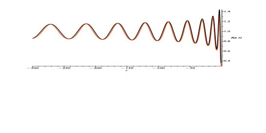
Figure 3: The red and black plots are, respectively, the real parts of the numeric and large-$r$ asymptotic values of the function $H(r)$ for $r\leqslant-0.6$ corresponding to the initial value $H(0)=-1/30-\mathrm{i}$.

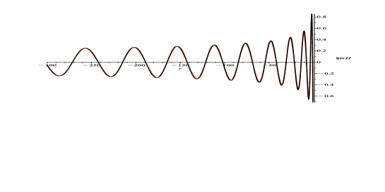
Figure 4: The red and black plots are, respectively, the imaginary parts of the numeric and large-$r$ asymptotic values of the function $H(r)$ for $r\leqslant-0.5$ corresponding to the initial value $H(0)=-1/30-\mathrm{i}$.

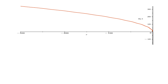
Figure 5: The red and black plots are, respectively, the real parts of the numeric and large-$r$ asymptotic values of $I=\smallint_{r}^{0}\tfrac{1}{\sqrt{-r}H(r)}\,\mathrm{d}r$ for $r\leqslant-10^{-7}$ corresponding to the initial value $H(0)=-1/30-\mathrm{i}$. On this scale, both plots almost coincide. In Figure 6, the reader will see a more detailed comparison of these plots.

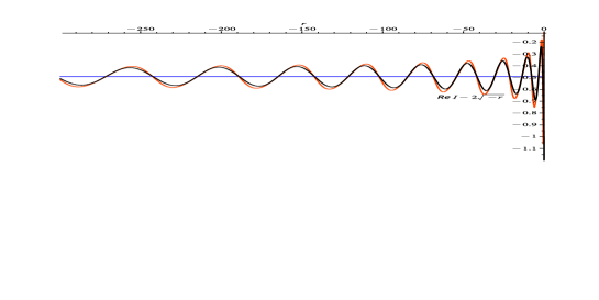
Figure 6: The red and black plots are, respectively, the real parts of the numeric and large-$r$ asymptotic values of $\smallint_{r}^{0}\tfrac{1}{\sqrt{-r}H(r)}\,\mathrm{d}r-2\sqrt{-r}$ for $r\leqslant-10^{-7}$ corresponding to the initial value $H(0)=-1/30-\mathrm{i}$. The blue line is the real part of the asymptotics (6.4) modulo the parabola $2\sqrt{-r}$ and $\mathrm{E}(r)$.

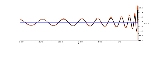
Figure 7: The red and black plots are, respectively, the imaginary parts of the numeric and large-$r$ asymptotic values of $\smallint_{r}^{0}\frac{1}{\sqrt{-r}H(r)}\,\mathrm{d}r$ for $r\leqslant-0.1$ corresponding to the initial value $H(0)=-1/30-\mathrm{i}$. The blue line is the imaginary part of the asymptotics (6.4) modulo $\mathrm{E}(r)$.

6.2 Example 2: $H(0)=60-\mathrm{i}100$

For this value of $H(0)$, $\nu_{1}=0.583250\ldots-\mathrm{i}0.162814\ldots$, so that the condition (6.3) is satisfied. Here, however, we are closer to the boundary of the interval of validity (6.3) for the asymptotics (6.1). For the Maple calculations, we choose the same settings as in Example 1. The results of these calculations are presented in Figs. 8–12: these $50$-digits calculations take approximately $133\text{s}$ on an older notebook (see footnote 8).

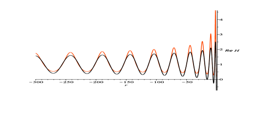
Figure 8: The red and black plots are, respectively, the real parts of the numeric and large-$r$ asymptotic values of the function $H(r)$ for $r\leqslant-0.6$ corresponding to the initial value $H(0)=60-\mathrm{i}100$

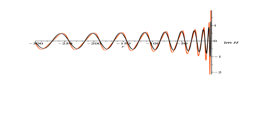
Figure 9: The red and black plots are, respectively, the imaginary parts of the numeric and large-$r$ asymptotic values of the function $H(r)$ for $r\leqslant-0.1$ corresponding to the initial value $H(0)=60-\mathrm{i}100$.

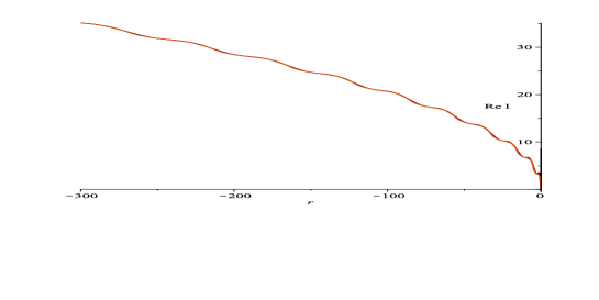
Figure 10: The red and black plots are, respectively, the real parts of the numeric and large-$r$ asymptotic values of $\smallint_{r}^{0}\tfrac{1}{\sqrt{-r}H(r)}\,\mathrm{d}r$ for $r\leqslant-10^{-6}$ corresponding to the initial value $H(0)=60-\mathrm{i}100$. Both plots virtually coalesce into one curve; however, one notices that this curve has some thick segments coloured in red from one side and in black from the other. A more detailed comparison of these plots is presented in Figure 11.

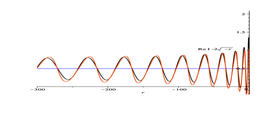
Figure 11: The red and black plots are, respectively, the real parts of the numeric and large-$r$ asymptotic values of $\smallint_{r}^{0}\frac{1}{\sqrt{-r}H(r)}\,\mathrm{d}r-2\sqrt{-r}$ for $r\leqslant-10^{-2}$ corresponding to the initial value $H(0)=60-\mathrm{i}100$. The blue line is the real part of the asymptotics (6.4) modulo the parabola $2\sqrt{-r}$ and $\mathrm{E}(r)$.

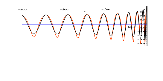
Figure 12: The red and black plots are, respectively, the imaginary parts of the numeric and large-$r$ asymptotic values of $\smallint_{r}^{0}\frac{1}{\sqrt{-r}H(r)}\,\mathrm{d}r$ for $r\leqslant-0.1$ corresponding to the initial value $H(0)=60-\mathrm{i}100$. The blue line is the imaginary part of the asymptotics (6.4) modulo $\mathrm{E}(r)$.

Remark 6.1.

In principle, the asymptotics (6.1) and (6.4) are valid even beyond the condition (6.3), that is, $|\text{Im}\,\nu_{1}|<1/2$; however, going farther and farther beyond the condition (6.3), the visual correspondence between the solution and its asymptotics is attained at larger and larger values of $|r|$. The correction terms to the asymptotics (6.1) and (6.4) (see Appendix C) improve the correspondence, but do not alter the general tendency: the correspondence between the numeric and asymptotic values for $H(r)$ and $I(r)$ deteriorates for finite, though quite large, values of $r$. As one approaches $|\text{Im}\,\nu_{1}|\approx 2/5$, the values of $r$ for which the visual correspondence is expected appear to be so large that it becomes unfeasible to calculate the solution for such values of $r$. This tendency is partially illustrated upon comparing Figs. 3 and 4 with Figs. 8 and 9, respectively, and the corresponding figures with the plots for the integrals: the visual correspondence worsens when the boundary value of the condition (6.3) is approached. Example 6 below illustrates at which values of $r$ one may expect to observe that the asymptotics (6.1) and (6.4) faithfully describe the large-$r$ behaviour of $H(r)$ and $I(r)$.

In order to cope with the problem indicated above, we derive in [27] yet another asymptotic formula which will be discussed below. $\blacksquare$

We now turn our attention to the numerical illustration of the asymptotic results for the function $H(r)$ that follow from Theorem C.2 (see Appendix C):

$$H(r)\underset{r\to-\infty}{=}1-\frac{3}{2\sin^{2}\left(\frac{1}{2}\hat{\psi}(r)+o\big{(}r^{-\delta}\big{)}\right)},\qquad\delta>0,$$ (6.6)

where

$$\hat{\psi}(r)=2\sqrt{-3r}+\left(\nu_{1}+\frac{\mathrm{i}}{2}\right)\ln\big{(}24\sqrt{-3r}\big{)}-\frac{\pi}{4}-\frac{3\pi\mathrm{i}}{2}\nu_{1}-\frac{\mathrm{i}}{2}\ln(2\pi)+\mathrm{i}\ln\big{(}\tilde{g}_{1}\Gamma(\mathrm{i}\nu_{1})\big{)},$$ (6.7)

$$\nu_{1}:=\frac{\ln{\tilde{g}_{3}}}{2\pi},\qquad\text{Im}\,\nu_{1}\in(-1,0)\setminus\{-1/2\}.$$ (6.8)

We draw the attention of the reader to the fact that, even though the parameter $\nu_{1}$ in (6.8) is defined by the same formula as $\nu_{1}$ in (6.3), its imaginary part is fixed in another interval. Clearly, both asymptotics (6.1) and (6.6) have intersecting domains of validity. The asymptotics for the integral $I(r)$ reads:

$$\int_{r}^{0}\frac{\mathrm{d}r}{\sqrt{-r}H(r)}\underset{r\to-\infty}{=}2\sqrt{-r}+(2\nu_{1}+\mathrm{i})\ln(2+\sqrt{3})+\pi(2k-1)+\mathrm{i}\ln\left(\frac{{H(0)\mathrm{e}^{\frac{2\pi\mathrm{i}}{3}}}-\mathrm{e}^{-\frac{2\pi\mathrm{i}}{3}}}{\mathrm{e}^{\frac{2\pi\mathrm{i}}{3}}-H(0)\mathrm{e}^{-\frac{2\pi\mathrm{i}}{3}}}\right)+\mathcal{E}(r),$$ (6.9)

where $k\in\mathbb{Z}$,

$$\mathcal{E}(r)=-\mathrm{i}\ln\left(\frac{\sin\big{(}\frac{1}{2}\hat{\psi}(r)+\theta_{0}+o\big{(}r^{-\delta}\big{)}\big{)}}{\sin\big{(}\frac{1}{2}\hat{\psi}(r)-\theta_{0}+o\big{(}r^{-\delta}\big{)}\big{)}}\right),\qquad\theta_{0}=-\frac{\pi}{2}+\frac{\mathrm{i}}{2}\ln\big{(}2+\sqrt{3}\big{)}.$$ (6.10)

Remark 6.2.

The number $k=k(H(0))\in\mathbb{Z}$ cannot be determined via the isomonodromy technique developed in [27] because, in fact, asymptotics of the function $\exp\left(\smallint_{r}^{0}\frac{1}{\sqrt{-r}H(r)}\,\mathrm{d}r\right)$ is studied there. It looks like an interesting problem to determine the integer $k$ in terms of the initial value $H(0)$. In the numerical examples considered below, we find $k$ by comparing the numerical solution for $H(r)$ with its asymptotics (6.9). Since $k$ is an integer, its experimental determination in this situation does not represent a problem. The values of $k$ are given in the corresponding figure captions. $\blacksquare$

Remark 6.3.

If $\text{Im}\,\nu_{1}\in(-1,-5/6)$, which corresponds to the range of validity of the asymptotics (6.6) and (6.9) (cf. condition (6.8)), then one can fix the branch of $\nu_{1}$ such that $\text{Im}\,\nu_{1}\in(0,1/6)$, so that the asymptotics (6.1) and (6.4) can be used; moreover, the closer $\text{Im}\,\nu_{1}$ is to $-1$ or to $0$, the better (in the sense of approximating $H(r)$ at finite values) work the asymptotics (6.1) and (6.4). $\blacksquare$

Remark 6.4.

This remark concerns the term $\mathcal{E}(r)$ in the asymptotic formula (6.9) (cf. (6.10)). It is assumed that one has to take a continuous branch of the logarithmic function as $r$ varies from $0$ to $-\infty$. This problem is important in numerical calculations because Maple calculates only the principal branch of the logarithmic function; therefore, plotting the asymptotic formula  (6.10) on a large-$r$ interval almost always produces a saw-like plot. To cope with this problem, one can present the logarithm in  (6.10) as an integral of the difference of cotangent functions. This idea works on small-length intervals; however, the calculation of this integral on the segment $[-10,0]$, say, already consumes a considerable amount of time, several times longer than the numerical calculation of the solution of the Painlevé equation itself! Consequently, in lieu of the integral, we define the continuous branch of the logarithm as the solution of the differential equation for the above-mentioned integral. It appears that Maple numerically evaluates this solution much faster than its explicit form represented by the integral in terms of cotangents. The execution time of this fast calculation, however, where only $20$-digits of accuracy were maintained, appears to be $5$ to $8$ times longer than the numerical calculation of the integral on the left-hand side of equation (6.9) based on its direct calculation (with $120$-digits of accuracy) via the Painlevé transcendent! There is, thus, a significant difference between the numerical calculations using the asymptotic formulae (6.4) and (6.9): plots of the first asymptotic formulae (6.4) are calculated almost immediately, whilst the second asymptotics (6.9) is interesting for theoretical studies until a fast algorithm for the calculation of continuous branches of the logarithmic functions will be implemented into Maple (and analogous codes). $\blacksquare$

Below, we consider several examples that illustrate some features of the asymptotic formulae (6.6) and (6.9).

6.3 Example 3: $H(0)=-0.148+\mathrm{i}0.191$

For this value of $H(0)$, $\nu_{1}=0.0249933\ldots-\mathrm{i}0.329580\ldots$, so that the condition (6.8) is satisfied, and we can use the asymptotic formulae (6.6) and (6.9). For the numerical calculation of the solution $H(r)$ and its related integral $I(r)$ via Maple, we consider the initial values for $H(r)$ at $r_{1}=10^{-8}$ and use 4 terms of the corresponding Taylor series expansions for the calculation of the initial values, $H(r_{1})$ and $H^{\prime}(r_{1})$, and the parameter Digits $=120$. For the calculation of the corresponding asymptotics, Digits is set equal to $20$. In principle, for the numerical calculation of $H(r)$ and $I(r)$, one can take a smaller number of digits, $60$, say, and the resulting calculation with $60$ digits produces visually the same pictures.

Figs. 13, 15, 17, and 19 demonstrate that the large-$r$ asymptotics also give quite good approximations for the corresponding functions even for small values of $r$. We took $800$ points for the calculation of these plots. The calculation from scratch of the numerical solution presented in Figure 17 with an older notebook (see footnote 8) takes $20\text{s}$, whilst the calculation of its asymptotics represented by the blue line of the same figure takes $170\text{s}$ (cf. Remark 6.4). In order to produce the numerical solution and the corresponding integral shown in Figs. 14, 16, 18, and 20 by the red curves, which are virtually concealed under the blue curves, a newer notebook (cf. footnote 8) requires $188\text{s}$ of execution time. The blue curves representing the asymptotic values were generated in approximately $1015\text{s}$ (cf. Remark 6.4). For the generation of these plots, we increased the number of points from $800$ to $1837$ because the plots have sharp peaks and the heights of the peaks depend substantially on the number and position of the points inside the peaks.

Figure 18 resembles a mole’s dwelling that can be reached with the aid of two ladders. The slopes of all the steps and risers of the left staircase are negative. The right staircase possesses steps with negative slopes and risers with positive slopes. Obviously, the sign of the slopes coincides with the sign of $-\mathrm{Re}\,(H(r))$. If we look at Figure 14, we observe, in fact, that the function $\mathrm{Re}\,(H(r))$ is negative on the segments near its local minima located near the origin; however, these minima are growing monotonically and slowly, as long as one moves in the negative direction, farther and farther away from the origin. What is not clearly seen from the figure, however, is the fact that the calculations show that the last segment where $H(r)<0$ occurs for $r\in(-414.68789\ldots,-398.07403\ldots)$, which corresponds to the right wall (first riser) of the mole’s dwelling. The left wall of the mole’s dwelling is the image of a segment around a local minimum at $r_{\mathrm{min}}=-482.3271\ldots$ where $H(r_{\mathrm{min}})=0.0022342881\ldots$. Due to the very small values of $|H(r)|$ on these segments, the walls look almost vertical, although, in fact, they have negative and positive slopes for the left and right walls, respectively.

Figure 13: The red and blue plots are, respectively, the real parts of the numeric and large-$r$ asymptotic (cf. (6.6)) values of the function $H(r)$ for $r\leqslant-0.1$ corresponding to the initial value $H(0)=-0.148+\mathrm{i}0.191$.

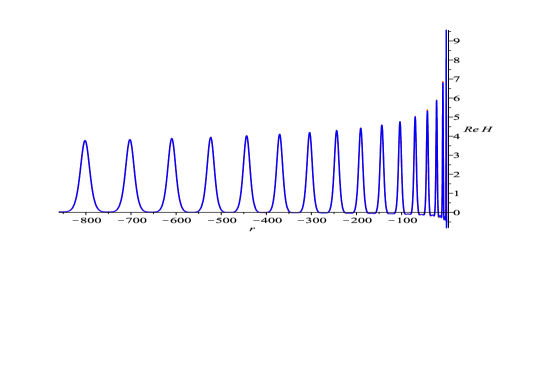
Figure 14: Extended version of Figure 13 (both plots almost coincide).

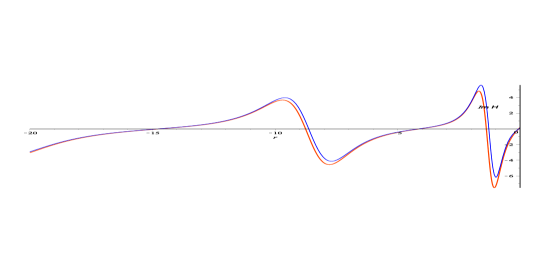
Figure 15: The red and blue plots are, respectively, the imaginary parts of the numeric and large-$r$ asymptotic (cf. (6.6)) values of the function $H(r)$ for $r\leqslant-0.01$ corresponding to the initial value $H(0)=-0.148+\mathrm{i}0.191$.

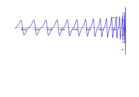
Figure 16: Extended version of Figure 15 (both plots almost coincide).

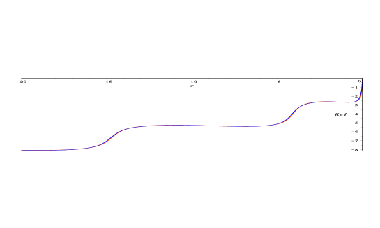
Figure 17: The red and blue plots are, respectively, the real parts of the numeric and large-$r$ asymptotic (cf. (6.9) with $k=0$) values of $I=\smallint_{r}^{0}\frac{1}{\sqrt{-r}H(r)}\,\mathrm{d}r$ for $r\leqslant-10^{-8}$, where $H(r)$ is the solution with initial value $H(0)=-0.148+\mathrm{i}0.191$. In black-and-white the curves are indistinguishable; in colour, though, one notices minor discrepancies between the curves.

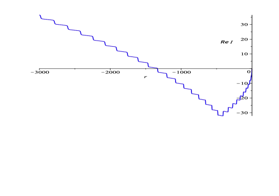
Figure 18: Extended version of Figure 17 (both plots almost coincide).

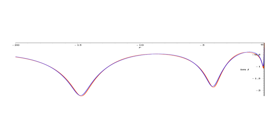
Figure 19: The red and blue plots are, respectively, the imaginary parts of the numeric and large-$r$ asymptotic (cf. (6.9) with $k=0$) values of $I=\smallint_{r}^{0}\frac{1}{\sqrt{-r}H(r)}\,\mathrm{d}r$ for $r\leqslant-10^{-3}$, where $H(r)$ is the solution with initial value $H(0)=-0.148+\mathrm{i}0.191$. In black-and-white some minor discrepancies between the curves are noticeable.

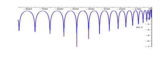
Figure 20: The red and blue plots are, respectively, the imaginary parts of the numeric and large-$r$ asymptotic (cf. (6.9)) values of $I=\smallint_{r}^{0}\frac{1}{\sqrt{-r}H(r)}\,\mathrm{d}r$ for $r\leqslant-10^{-3}$ corresponding to the solution $H(r)$ with initial value $H(0)=-0.148+\mathrm{i}0.191$. On a coloured figure one can see that the three red peaks on the segment $[-600,-400]$ are slightly (less than $5$%) longer than the blue ones, whilst the differences between the lengths of the other corresponding red and blue peaks are virtually indistinguishable.

In Example 3, we demonstrated that, for some initial vales of $H(r)$, the leading terms of the large-$r$ asymptotics approximate very closely the corresponding Painlevé function and its related integral starting from very small values of $r$ ($r<1$). In Example 4 below, we show that there are markedly different initial values of $H(r)$ for which $H(r)$ and its related integral have behaviour similar to that seen in Example 3; however, an approximation for small values of $r$ becomes considerably worse, even though it remains satisfactory in the qualitative sense; moreover, in order to achieve the correct plots, one has to be much more cautious with the numerical settings.

6.4 Example 4: $H(0)=-100-\mathrm{i}300$

For this value of $H(0)$, $\nu_{1}=0.741160\ldots-\mathrm{i}0.300731\ldots$, so that the condition (6.8) is satisfied, and we can use the asymptotic formulae (6.6) and (6.9). For the numerical calculation of the solution and its related integral via Maple, we consider the initial values for $H(r)$ at $r_{1}=10^{-9}$. For the calculation of the initial values of $H(r)$ and its corresponding integral, we use 6 terms of the Taylor expansion for $H(r)$ (cf. Section 2, equations (2.1), (2.2), and (2.17)). For visualisation purposes, 4 terms for $H(r)$ and 2 terms for $I(r)$ of the Taylor series expansion are, in principle, sufficient. We set the parameter Digits $=180$, and the same value $180$ was set for the calculation of asymptotics. This large value $180$ for the parameter Digits is important for the calculation of the imaginary part of the asymptotic formulae, because, as explained above, the logarithmic term in the asymptotics (6.10) for the integral is calculated via a solution of an appropriate differential equation. Somehow, in Example 3, for the calculation of the asymptotics, we kept Digits equal to $20$ and did not notice visual differences while increasing its value. In this example, however, we found a difference when the value of Digits was increased from 20 to $100$. To verify that the plots remain stable, we increased Digits up to $180$: the plots presented below correspond to this value of the parameter Digits. In principle, $80$ to $90$ digits for this calculation suffices.

For the generation of the plots with ‘peaks’, we found that the most appropriate value for the number of points was $5237$, while in Example 3, this value was kept at $1837$. In this example, we were obliged to keep it that high because the height of the three highest peaks were not stable until the number of points reached the value $5237$, after which, these heights underwent only minor variations. The calculation with that many digits and number of points increases the required time by about $20\%$, which, in our case, is not crucial.

In Example 3, we explained that the ‘staircase-structure’ of the plot for $\mathrm{Re}\,I(r)$ is a consequence of the fact that the tail of the numeric plot for $\mathrm{Re}\,H(r)$ is floating slowly upwards from the third to the second quadrant as $r\to-\infty$; the same behaviour, of course, is replicated in its asymptotic plot. If the tails of both plots float above the negative real axis almost simultaneously, then the numeric and asymptotic mole dwellings almost coincide (cf. Figure 18). The rate of floating of the tails, however, depends on the initial value $H(0)$. It may happen (and in many cases it does) that, although both plots are very close to one another, as in the present case, one tail (the red one) floats before the other (the blue one); in Figure 22, the red tail floats at $r\approx-55$, prior to the fifth peak, while the blue tail floats at $r\approx-120$, prior to the seventh peak. Due to scaling, this fact is not clearly seen in Figure 22, but we verified it numerically. Thus, the upward-trending float of the asymptotic tail lags the numeric one by two peaks, so that the ‘asymptotic’ mole’s dwelling appears to be two steps lower than the ‘numeric’ dwelling (cf. Figure 27). This example demonstrates that the integer $k$ in the asymptotic formula (6.9) for $I(r)$ appears not only because this formula originates from the asymptotics of the function $\varphi(r)$, which is defined modulo $2\pi k$ (cf. Appendix B), but also because it is related to the quality of the approximation of the numeric plot by its asymptotics at finite values of $r$. Note that the parameter $k$ undergoes a shift of $2$ when one approximates the small-$r$ part of the numeric solution and its large-$r$ part via the asymptotics (6.9) (cf. Figs. 27 and 25, respectively).

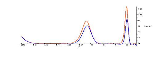
Figure 21: The red and blue plots are, respectively, the real parts of the numeric and large-$r$ asymptotic (cf. (6.6)) values of the function $H(r)$ for $r\leqslant-0.1$ corresponding to the initial value $H(0)=-100-\mathrm{i}300$.

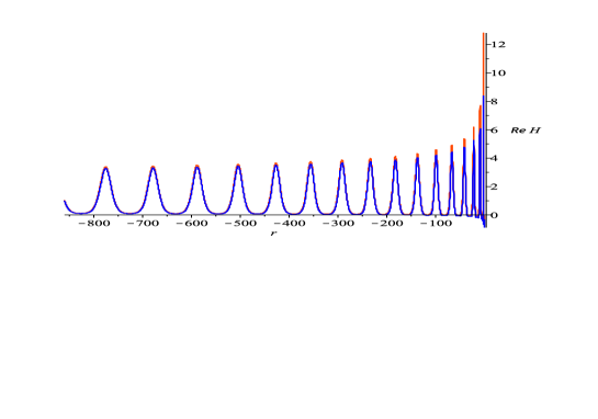
Figure 22: Extended version of Figure 21, where only the first two peaks are shown. On this plot, the first peak virtually coincides with the vertical axis.

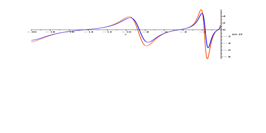
Figure 23: The red and blue plots are, respectively, the imaginary parts of the numeric and large-$r$ asymptotic (cf. (6.6)) values of the function $H(r)$ for $r\leqslant-0.1$ corresponding to the initial value $H(0)=-100-\mathrm{i}300$.

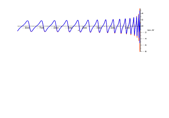
Figure 24: Extended version of Figure 23. On this plot, the first down-up peak of Figure 23 almost coincides with the vertical axis.

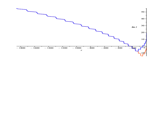
Figure 25: The red and blue plots are, respectively, the real parts of the numeric and large-$r$ asymptotic (cf. (6.9) with $k=3$) values of $I=\smallint_{r}^{0}\frac{1}{\sqrt{-r}H(r)}\,\mathrm{d}r$ for $r\leqslant-10^{-8}$ corresponding to the solution $H(r)$ with initial value $H(0)=-100-\mathrm{i}300$.

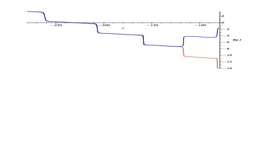
Figure 26: A close-up of the segment of the plot on Figure 25 corresponding to $-280\leqslant r\leqslant-80$ where the numeric and asymptotic plots merge at $r\approx-120$. One can actually distinguish two different intertwining (for $r<-120$) curves which are very close to each other.

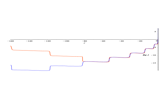
Figure 27: A close-up of the part of the plot of the numerical solution on Figure 25 for $-160<r<-10^{-9}$ and the corresponding asymptotic plot (cf. (6.9) with—attention!—$k=1$). One can actually distinguish two separate intertwining curves which are very close to one another. The ‘numeric’ mole’s dwelling corresponds to $r\in(-80,-55)$, while the ‘asymptotic’ dwelling is located two steps below with $r$-coordinate in $(-160,-120)$.

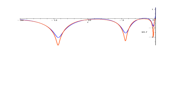
Figure 28: The red and blue plots are, respectively, the imaginary parts of the numeric and large-$r$ asymptotic (cf. (6.9): $k$ is not important here) values of $I=\smallint_{r}^{0}\frac{1}{\sqrt{-r}H(r)}\,\mathrm{d}r$ for $-20\leqslant r\leqslant-10^{-9}$ corresponding to the solution $H(r)$ with initial value $H(0)=-100-\mathrm{i}300$.

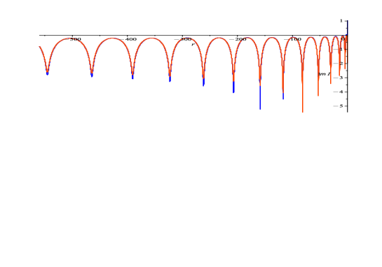
Figure 29: Extended version of Figure 28 for $-560\leqslant r\leqslant-10^{-9}$. Here, the first peak on Figure 28 virtually coincides with the vertical axis, and is therefore not clearly visible. The first 6 icicles of the numerical solution are longer than the corresponding asymptotic icicles; however, from the 7th icicle onward, the asymptotic icicles are longer, but the difference between the corresponding icicles decreases rapidly.

6.5 Example 5: $H(0)=-\mathrm{i}300$

For this value of $H(0)$, $\nu_{1}=0.732934\ldots-\mathrm{i}0.249469\ldots$, so that the condition (6.8) is satisfied, and we can use the asymptotic formulae (6.6) and (6.9). For the numerical calculation of the solution and its related integral via Maple, we used the same settings as in Example 4. In this case, the plots look similar to those in Example 4. The difference in this example is that, for $r<0$, $\mathrm{Re}\,H(r)>0$; however, for small values of $r$, $\mathrm{Re}\,H(r)$ is very close to zero; for example, at the first minimum $r_{\mathrm{min}}=-0.485998\ldots$, $H(r_{\mathrm{min}})=0.024587\ldots$ (cf. Figure 30). As in Example 4, the approximation for $H(r)$ via its large-$r$ asymptotics is not as good as that for the initial data for which $10^{-3}<|H(0)|<10^{3/2}$. For small values of $r$, though, there are two segments wherein the asymptotics for $\mathrm{Re}\,H(r)$ is negative (cf. Figure 30). These facts imply that the numerical plot for $I(r)$ looks similar to the plot of Figure 10 (no mole’s dwelling (!)); however, the plot for the asymptotics does, indeed, contain two descending steps to the numerical plot of $I(r)$ until they merge. So, in lieu of the mole’s dwelling, we have an ‘asymptotic pigeon hole’. On the segment $[-5.5,0]$, the asymptotic formula does not even approximate qualitatively the solution.

When we increase the value of $|\mathrm{Im}\,H(0)|$, the asymptotic pigeon hole shifts to the left; for $H(0)=-\mathrm{i}10^{5}$, say, the asymptotic pigeon hole is located on the segment $[-79,-59]$, and, as a result, the asymptotics does not approximate $I(r)$ on $[-59,0]$. Our numerical experiments show that, in this case, a good approximation for $I(r)$ on the segment $[-79,-3]$ is attained by a reflection of the asymptotic plot with respect to a straight line passing through two points at the bottom of the asymptotic pigeon hole. These two points are not uniquely defined; therefore, one may vary the location of these points in order to achieve a better approximation.

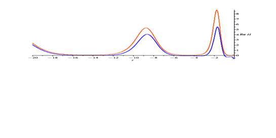
Figure 30: The red and blue plots are, respectively, the real parts of the numeric and large-$r$ asymptotic (cf. (6.6)) values of the function $H(r)$ for $r\leqslant-0.1$ corresponding to the initial value $H(0)=-\mathrm{i}300$. The numeric solution (in red) is positive, while the asymptotic solution (in blue) has two segments where it is negative.

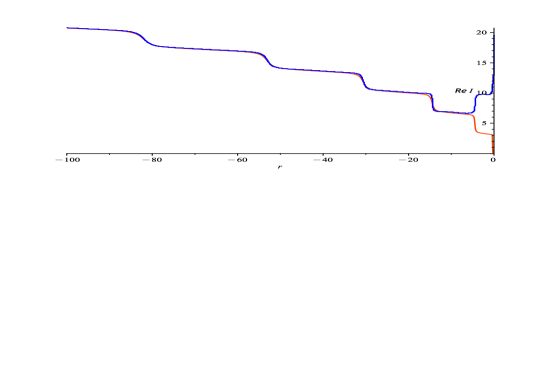
Figure 31: The numerical solution (in red) merges with the asymptotic (cf. (6.9) with—attention!—$k=3$) solution (in blue) on the segment $(-6,-5.5)$. The right-most point of both plots is $r=-10^{-9}$.

6.6 Example 6: $H(0)=-0.2+\mathrm{i}0.045$

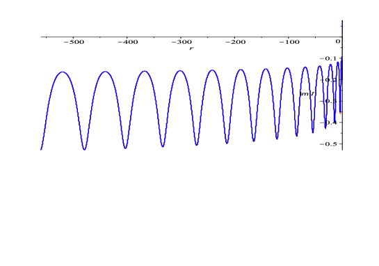
Figure 39: Extended version of Figure 38 for $r\leqslant-10^{-5}$. In this figure, the first peak of Figure 38 almost coincides with the vertical axis, and is therefore not clearly visible. At the end-points of the first few peaks, one can distinguish small red dots.

For this value of $H(0)$, $\nu_{1}=0.049319\ldots-\mathrm{i}0.459650\ldots$, so that the condition (6.8) is satisfied, and we can use the asymptotic formulae (6.6) and (6.9). For the numerical calculation of the solution and its related integral via Maple, we used the same settings as in Example 4. The plots presented in Figs. 32–39 were generated in $957\text{s}$ with the help of the newer notebook described in footnote 8.

It is instructive to compare this example with Example 3: the initial values in both examples are close, but the behaviour of the solutions is very different. This occurs because, in Example 6, $\textrm{Im}\,\nu_{1}$ is much closer to $-0.5$. This last fact also causes the appearance of very sharp peaks in the plots for the real and imaginary parts of $H(r)$. These peaks create an additional problem for the visualization of asymptotics because we were not able to obtain the right heights for the first peaks in our plots: not even 15000 points for constructing the plots was sufficient! Our strategy is two-fold: (i) we consider two close-up plots for $\textrm{Re}\,H(r)$ and $\textrm{Im}\,H(r)$ (cf. Figs. 32 and 34) in order to determine the correct heights of the first two peaks; and (ii) to construct the extended plots (cf. Figs. 33 and 35) we randomly choose the number of points in order to get the heights of the first two peaks to be as close as possible, like in the close-up figures. For item (i), we used 5237 and 1800 points for the construction of the plots in Figs. 32 and 34, respectively. In this case, the heights of the first two peaks of the real part of the numerical solution were found to be approximately 182 and 121, respectively. On the extended version of Figure 32 (cf. Figure 33), the best possible heights that we were able to achieve were 163 and 119, respectively, with the number of points equal to 6237. To get good correspondence between the peaks on the close-up and extended figures for the imaginary part of the numerical solution, we constructed the extended plot with the help of 10800 points. For the corresponding asymptotic plots, 2200 points was enough for both cases. The real part of $I(r)$ does not have any sharp peaks, so we used 1800 points. The imaginary part of $I(r)$ has only one sharp peak for small negative $r$, and we achieved its right height with 5237 points for both the numerical and asymptotic plots.

An intriguing feature of this example is that, practically, it is not possible to reach the mole’s dwelling by numerically calculating $I(r)$. Our calculation reveals that the last zero of $\mathrm{Re}\,H(r)$ is located at $\approx-2.625\times 10^{24}$: the right wall of the mole’s dwelling is located at this point, and what is termed ‘asymptotics’ only begins here! Therefore, practically speaking, it is not possible to numerically generate a plot for the solution and verify that, finally, the leading term of asymptotics is given by a shifted parabola $2\sqrt{-r}$, i.e., the non-oscillatory part of the asymptotics (6.4). We see, however, that the asymptotic formula (6.9) very well describes the right staircase leading to the mole’s dwelling starting from the first step; therefore, the asymptotics (6.9) is correct, from which it follows that, for very large negative values of $r$, the solution should behave like the shifted parabola $2\sqrt{-r}$. This illustrates the theoretical application of the asymptotic formula (6.9) mentioned in Remark 6.4; without knowledge of the asymptotics, one may assume that the right staircase constitutes the asymptotic behaviour of $I(r)$ for all large negative $r$.

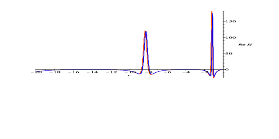
Figure 32: The red and blue plots are, respectively, the real parts of the numeric and large-$r$ asymptotic (cf. (6.6)) values of the function $H(r)$ for $r\leqslant-0.1$ corresponding to the initial value $H(0)=-0.2+\mathrm{i}0.045$.

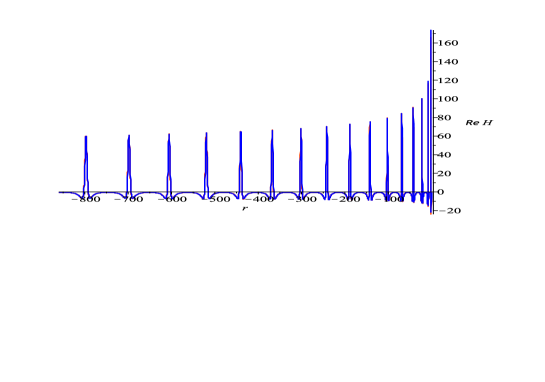
Figure 33: Extended version of Figure 32 where the first two peaks of the plot are shown. On this plot, the first peak almost coincides with the vertical axis.

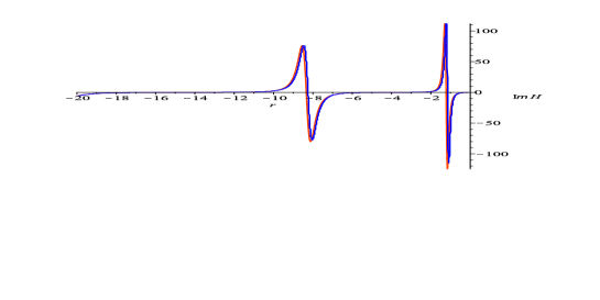
Figure 34: The red and blue plots are, respectively, the imaginary parts of the numeric and large-$r$ asymptotic (cf. (6.6)) values of the function $H(r)$ for $r\leqslant-0.1$ corresponding to the initial value $H(0)=-0.2+\mathrm{i}0.045$.

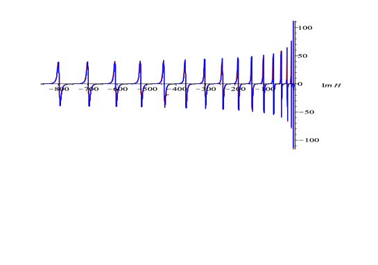
Figure 35: Extended version of Figure 34. On this plot, the first down-up peak of Figure 34 virtually coincides with the vertical axis.

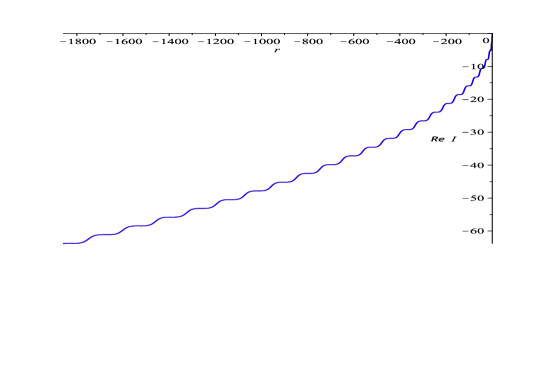
Figure 36: The red and blue plots are, respectively, the real parts of the numeric and large-$r$ asymptotic (cf. (6.9) with $k=0$) values of $I=\smallint_{r}^{0}\frac{1}{\sqrt{-r}H(r)}\,\mathrm{d}r$ for $r\leqslant-10^{-8}$ corresponding to the solution $H(r)$ with initial value $H(0)=-0.2+\mathrm{i}0.045$. The red plot is overlapped by the blue plot, and is therefore not visible. On the close-up Figure 37 that follows, one can distinguish the red colour.

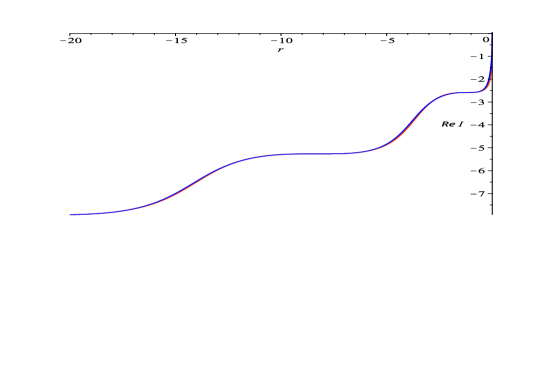
Figure 37: A close-up of a part of the plot of the numerical solution in Figure 36 for $-20\leqslant r\leqslant-10^{-8}$, and the corresponding asymptotic plot (cf. (6.9) with $k=0$). On the coloured picture, one can see that the steeper slopes from below are in red while those from above are in blue.

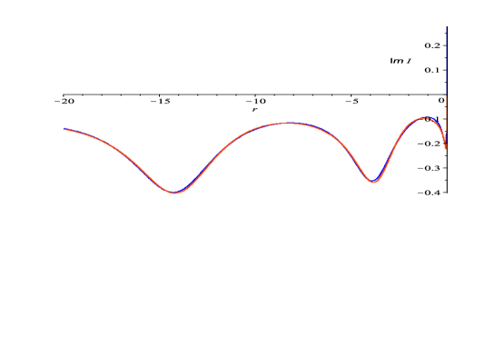
Figure 38: The red and blue plots are, respectively, the imaginary parts of the numeric and large-$r$ asymptotic (cf. (6.9)) values of $I=\smallint_{r}^{0}\frac{1}{\sqrt{-r}H(r)}\,\mathrm{d}r$ for $-20\leqslant r\leqslant-10^{-9}$ corresponding to the solution $H(r)$ with initial value $H(0)=-0.2+\mathrm{i}0.045$.

Remark 6.5.

Question: Where is the mole’s dwelling in Figure 36? Answer: No one can see it, but it exists! As explained in Example 3, the location of the dwelling (its right wall) corresponds to the last zero of the function $\mathrm{Re}\,H(r)$. Observing Figure 33, one may have a concern as to whether or not this last zero does, in fact, exist, because we see that the asymptotic formula (6.6) works very well within the given plot, and we expect that it should replicate, with minor changes, as $r\to-\infty$. The major tendency of the large-$r$ behaviour of the solution that follows from Figure 33 is that the heights of the peaks becoming lower and the distances between them increase. Another tendency in the transformation of the plot which is more subtle, however, is that its tail is floating up slowly above the negative real semi-axis as one proceeds to the the left ($r\to-\infty$): finally, $\mathrm{Re}\,H(r)\to 1$; therefore, the last zero of $\mathrm{Re}\,H(r)$ should exist.

In order to comprehend these tendencies, one has to consider the asymptotics of the asymptotic formula (6.6): equation  (6.6), in fact, can be simplified and transformed into an expression resembling the “regular asymptotics” (6.1); so, in this sense, the latter asymptotics serves as “the asymptotics of asymptotics”. This is reasonable terminology, because the beginning of the plot where the first asymptotics (6.6) is already working, and the tail of the plot, where it is, of course, still working, look radically different! At the same time, though, we explain below that, practically, one cannot visualize this difference!

The plots in Figs. 32 and 33 show that the asymptotics accurately approximates $\mathrm{Re}\,H(r)$; as a result, for the calculation of the last zero of $\mathrm{Re}\,H(r)$, we can use the asymptotics of this function instead of its numerical evaluation. This is important because, as is evident from the result (6.11) stated below, such a calculation is not possible due to the “astronomical distances” required for this purpose. According to our calculations, the last zero of $\text{Re}\,H(r)$ is located at

$$r_{0}=-2.6279340765216450944920718115\ldots\times 10^{24}.$$ (6.11)

On the plot of $\mathrm{Re}\,I(r)$, after the point, $r_{0}$, one steps onto the floor of the mole’s dwelling, from which the left stairway to heaven begins. In order to evaluate the depth where the dwelling is located, one has to count the number of zeros of $\text{Re}\,H(r)$. In Figure 33, we see that the plot has a quasi-periodic structure: by quasi-period we mean a part of the plot located between two neighbouring peaks. Each peak “stands” on two legs, so that one leg of a peak belongs to the left quasi-period, whereas the other leg belongs to the right quasi-period; therefore, each leg intersects the negative real axis, and gives rise to one zero of $\text{Re}\,H(r)$. Thus, each quasi-period has at least two zeros. There is one more point that requires verification, namely, the maximum point on the “bridge” connecting the legs. This point is always negative until one arrives at the quasi-period with the last zero. It is evidently not a trivial matter to establish this for the Painlevé function; however, it can be proved for its asymptotics (6.6). Numerically, for the first two quasi-periods shown in Figure 32, we found that $r_{\max,1}=-3.756\ldots$, with $H(r_{\max,1})=-0.46471\ldots$, and $r_{\max,2}=-14.118\ldots$, with $H(r_{\max,2})=-0.47042\ldots$. So, the floating process of the tail evolves as follows: the legs are lifting up and the distance between them is growing at the same time that the “bridge” between the legs straightens out so that its maximum point is moving down. Thus, the shape of the bridge changes from convex to concave, the legs disappear, the maximum turns smoothly to the minimum, and the floating process continues: the tail (on some appropriate scale) becomes similar to the plot shown in Figure 14. This transformation of the plot is progressing very slowly on astronomically large distances for $|r|$; however, it can still be observed with the help of the asymptotic formula (6.6). At this stage of the evolution, the transformation of the plot continues: the spikes become more and more “plateaued”, so that, finally, the tail, after an appropriate re-scaling, resembles the black plot in Figure 1. Practically, the graph of this part of the tail cannot be plotted even with the help of asymptotics, because the distance between the spikes, as well as the spikes themselves, are becoming progressively more and more stretched along the negative semi-axis, unless some special scaling for $r$ is used which changes concomitant with the growth of $|r|$.

Reverting back to the determination of the mole’s dwelling, we note that the pair of zeros between two neighbouring peaks of $\mathrm{Re}\,H(r)$ correspond to one step down in the right staircase. If $2N$ denotes the number of zeros, then there are $N$ steps down in the right staircase. The depth of each step-down, starting from the second one, should be $\pi$, so that the depth of the mole’s dwelling, for large $N$, is $\pi N+\mathcal{O}(1)$. On the other hand, this depth can be calculated (cf. equations (6.9) and (6.10)) as follows, $\mathrm{Re}\big{(}(\hat{\psi}(r_{0})-\theta_{0})/2+(\hat{\psi}(r_{0})+\theta_{0})/2\big{)}-2\sqrt{-r_{0}}+o(1)$, so that, for large $|r_{0}|$, mole’s dwelling is located at a depth of about $2\sqrt{-3r_{0}}-2\sqrt{-r_{0}}+\mathcal{O}\big{(}\ln\sqrt{-3r_{0}}\big{)}$. A more careful estimation requires the $\mathcal{O}(1)$ contribution which, on the scale of our distances (6.11), is comparable to the logarithmic error estimate; but, for the purposes of the rough evaluation we are looking for, such contributions do not matter. Numerically, for the $y$-co-ordinate of the mole’s dwelling, we get the following estimate:

$$-2(\sqrt{3}-1)\sqrt{-r_{0}}=-2.373441069108\ldots\times 10^{12}.$$ (6.12)

We expect that $10$ to $11$ digits after the decimal point in (6.12) are correct. A more careful estimate for the depth of the mole’s dwelling can be obtained with the help of the so-called stair-stringer (6.14) discussed in the following subsection. $\blacksquare$

6.7 Stair-Stringers

In conclusion, we would like to formulate some observations concerning the asymptotic behaviour of $I(r)$. These observations require further investigations and more careful formulations. In Examples 1 and 2, the real part of $I(r)$ looks like a staircase. In Examples 3–6, we observe two staircases connected with the mole’s dwelling. The appearance of the mole’s dwelling on the plot of $I(r)$ was explained in terms of the floating of the tail of the plot of the function $H(r)$ above the negative-$r$ semi-axis. We conjecture that the straight line $H_{-}(r)=-1/2=\operatorname{Re}\big{(}\mathrm{e}^{\pm 2\pi\mathrm{i}/3}\big{)}$ plays the role of an unstable attracting line, and the appearance of the mole’s dwelling and its location can be explained via the interaction of the stable attracting line, $H_{+}(r)=+1$, and the unstable attracting line, $H_{-}(r)$.

By the term stair-stringer we mean the non-oscillatory part of the leading term of asymptotics describing the staircases. The stair-stringer for the left staircase, denoted by $Str_{l}$, can be deduced immediately from the asymptotics (6.4), namely,

$$Str_{l}=2\sqrt{-r}+2\mathrm{Re}(\nu_{1})\ln(2+\sqrt{3})+2\pi k-\mathrm{Im}\left(\ln\left(\frac{\mathrm{e}^{\frac{2\pi\mathrm{i}}{3}}H(0)-\mathrm{e}^{-\frac{2\pi\mathrm{i}}{3}}}{\mathrm{e}^{\frac{2\pi\mathrm{i}}{3}}-H(0)\mathrm{e}^{-\frac{2\pi\mathrm{i}}{3}}}\right)\right).$$ (6.13)

To get a formula for the stair-stringer for the right staircase, denoted by $Str_{r}$, is more complicated; however, the assiduous reader of this section should be able to derive the following formula:

$$Str_{r}= -2(\sqrt{3}-1)\sqrt{-r}-\mathrm{Re}(\nu_{1})\ln\sqrt{-r}+\mathrm{Re}(\nu_{1})\ln\left(\frac{(2+\sqrt{3})^{2}}{(2\sqrt{3})^{3}}\right)-\frac{3\pi}{2}\mathrm{Im}(\nu_{1})$$ (6.14)

$$+\frac{\pi}{4}+2\pi(k-1)-\mathrm{Im}\left(\ln\left(\frac{\mathrm{e}^{\frac{2\pi\mathrm{i}}{3}}H(0)-\mathrm{e}^{-\frac{2\pi\mathrm{i}}{3}}}{\mathrm{e}^{\frac{2\pi\mathrm{i}}{3}}-H(0)\mathrm{e}^{-\frac{2\pi\mathrm{i}}{3}}}\right)\right)+\mathrm{Im}\left(\ln\left(\tilde{g}_{1}\Gamma(\mathrm{i}\nu_{1})\right)\right).$$

In equations (6.13) and (6.14), $k\in\mathbb{Z}$ is an explicit manifestation of the $2\pi$-indeterminacy of the imaginary part of the asymptotics (6.4) and (6.9).

The stair-stringer $Str_{l}$ does not require additional visualization since it is a major part of the leading term of asymptotics which has already been verified in Examples  1 and 2. The “intermediate” stair-stringer $Str_{r}$ is illustrated with the help of Figs. 40 and 41: the integer $k$ in both of these figures is equal to $1$, while $k=0$ for $Str_{r}$ corresponding to Example 6, which is not presented here.

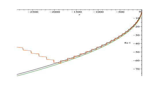
Figure 40: The red curve represents the numerical values of $\mathrm{Re}\,I(r)$ corresponding to the initial value $H(0)=-0.4+\mathrm{i}0.78$. The Maple settings for the generation of this curve are similar to those of Example 6. The parameter $\nu_{1}$ for this solution equals $-0.396664\dotsc-\mathrm{i}0.198139\dotsc$. The black line represents $Str_{r}$ with $k=1$, and the lowest (green) line is the unstable attracting parabola.

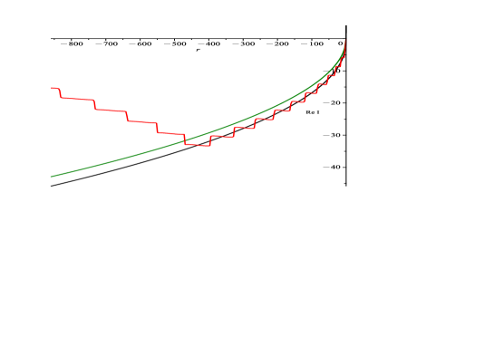
Figure 41: The red curve represents the numerical values of $\mathrm{Re}\,I(r)$ corresponding to the initial value $H(0)=-100-\mathrm{i}200$. The Maple settings for the generation of this curve are similar to those of Example 4. The parameter $\nu_{1}$ for this solution equals $0.686841\dotsc-\mathrm{i}0.323156\dotsc$. The black line represents $Str_{r}$ with $k=1$, and the upper (green) line is the unstable attracting parabola.

The asymptotic behaviour as $r\to-\infty$ of almost all solutions of equation (1.2) (in particular, all solutions considered in this work) can be described as follows: there exists some $r$ which could be small or large, depending on a solution, such that solutions are attracted to the parabola $2\sqrt{-r}$ and remain oscillatory at a distance (cf. (6.13)) $Str_{l}-2\sqrt{-r}$ which can be small or large, depending on a particular solution. In this sense, we can call $r\to 2\sqrt{-r}$ the stable attracting parabola. Many solutions, prior to their behaviours being equilibrated by the stable attracting parabola, are being “captured” by the unstable attracting parabola, that is, $r\to-2(\sqrt{3}-1)\sqrt{-r}$. For any $r=r_{0}$, there is a solution which is attracted by the unstable parabola on the distance $|r_{0}|$. These solutions are oscillating near $Str_{r}$. Contrary to the case for $Str_{l}$, the distance between the unstable parabola and $Str_{r}$ has logarithmic growth; however, this growth is not the reason why the unstable parabola cannot hold the solution on the infinite-$r$ interval. Our formal explanation for this behaviour of the solutions, which relies on the notion of ‘asymptotics of asymptotics’, is given in Remark 6.5; it implies that the tail of the plot for $\textrm{Re}\,H(r)$ is floating above the negative real semi-axis, and therefore the number of down-steps should be finite.

The function $\mathrm{Re}\,I(r)$ can serve as a mathematical model describing the mole’s behaviour. This model gives a simpler and even more convincing explanation for the instability of the right parabola. The mole is moving leftward-downward leaving behind a trajectory resembling the right staircase; the deeper and deeper the mole burrows, the less and less food it finds, so that the right staircase becomes less and less concave. Finally, the mole realizes that there is no food. At this stage, the mole constructs its dwelling, and, after a brief respite gathering its thoughts, the mole, regardless of its nature, realizes that it is necessary to change its direction of movement, and, finally, does so! Consequently, the mole starts to build the left staircase. Initially, the mole moves up in a near-vertical manner; however, since it is difficult to move vertically, its trajectory becomes “wavy”. After a few steps, the mole sees more and more food in front of itself, thus its horizontal motion becomes longer and longer, whilst its vertical movement continues to shrink; hence, the left staircase becomes less and less convex. Depending on the particular situation, regulated by the value of $H(0)$, the location of the mole’s dwelling will be different. We can also interpret the steps of the staircase as tunnels made by the mole, the lengths of which can be regulated with the help of a scaling parameter, $c>0:r\to cr$. What about the imaginary part of $I(r)$? We see (cf. Figure 20) that each icicle corresponds to a step/tunnel in its own right. We know that the mole is making repositories for its food; so, in each tunnel there is a single food repository, and the lengths of the icicles can be interpreted as numbers that are proportional to the food supply accrued in the corresponding repositories. In accordance with this model, the largest repository of food is located precisely in the mole’s dwelling.

A more interesting model describing the “underground mole’s geometry” could be related to a generalization of the function $I(r)$ that depends on two variables. It seems plausible, therefore, to “dig” for such a function amongst the integrals associated with the higher Painlevé equations depending on two variables, namely, the second member of a hierarchy related to the degenerate third Painlevé equation (1.1).

Appendix A Appendix: The Function $g_{2}(r)$

In Section 2, the definition of the generating functions $g_{k}(r)$, $k=1,2,\dotsc$, are given, and the first function of this sequence, $g_{1}(r)$, is constructed. The second function, $g_{2}(r)$, is constructed here, and we also explain how one calculates $P_{n}^{{}^{\prime}}(-1)$ with the help of this result.

The differential equation for $g_{2}(r)$ is

$$\big{(}rg_{2}^{{}^{\prime}}(r)\big{)}^{\prime}=3g_{2}(r)-\frac{1}{3}+\frac{1}{3}\big{(}I_{1}(2\sqrt{3r})\big{)}^{2},$$ (A.1)

where $I_{1}$ is the modified Bessel function of order $1$. This ODE is an inhomogeneous modified Bessel equation of order $0$. The small-$r$ expansion of $g_{2}(r)$ does not contain logarithmic terms, and its leading term is $-r/3$. This fact allows us to uniquely specify the proper solution of this equation:

$$g_{2}(r)=\frac{1}{9}-\frac{1}{9}I_{0}(2\sqrt{3r})+\frac{2}{3}\int_{0}^{r}\left(I_{0}(2\sqrt{3r})K_{0}(2\sqrt{3x})-K_{0}(2\sqrt{3r})I_{0}(2\sqrt{3x})\right)\left(I_{1}(2\sqrt{3x})\right)^{2}\mathrm{d}x.$$ (A.2)

The following expansion is not widely known; however, it is very helpful in our study:

$$\left(I_{1}(2\sqrt{3x})\right)^{2}=3x\sum_{n=0}^{\infty}\frac{\binom{2n+2}{n}(3x)^{n}}{((n+1)!)^{2}},$$ (A.3)

where $\tbinom{m}{k}=\tfrac{m!}{k!(m-k)!}$ is the binomial coefficient.

Since, in fact, we need the Taylor series expansion of $g_{2}(r)$, we solve equation (A.1) with the help of power series. Substituting the expansion

$$g_{2}(r)=\sum_{k=1}^{\infty}c_{k}\,r^{k},$$ (A.4)

where the coefficients $c_{k}$, $k=1,2,\ldots$, are independent of $r$, into equation (A.1), one deduces the following recurrence relation,

$$(k+1)^{2}c_{k+1}=3c_{k}+\frac{3^{k-1}}{(k!)^{2}}\binom{2k}{k-1},\quad c_{1}=-\frac{1}{3}.$$

Solving the last relation, we find that

$$c_{n}=\frac{3^{n-2}}{(n!)^{2}}\left(-1+\sum_{k=1}^{n-1}\binom{2k}{k-1}\right),\quad n=1,2,\ldots.$$ (A.5)

Remark A.1.

The integer sequence $\sum_{k=1}^{n-1}\binom{2k}{k-1}$, $n=2,3,\ldots$, coincides with sequence A057552 in [24]. Shifting $n$ to $n-2$ in a formula given in [24], we find that

$$\sum_{k=1}^{n-1}\binom{2k}{k-1}=\frac{\binom{2n-2}{n-1}}{2n}\left(4n-2-n\,{}_{2}F_{1}(1,-n+1;-n+3/2;1/4)\right)-\frac{1}{2},\quad n\in\mathbb{N},$$

where ${}_{2}F_{1}(1,-n+1;-n+3/2;1/4)$ is the value of the Gauss hypergeometric function at $x=1/4$, and $\tfrac{\binom{2n-2}{n-1}}{n}$ is the $(n-1)$th Catalan number. It is interesting to note that Maple gives a more complicated presentation for this sum:

$$\sum_{k=1}^{n-1}\binom{2k}{k-1}=-\frac{1}{2}+\frac{\mathrm{i}\sqrt{3}}{6}-\binom{2n}{n-1}\,{}_{3}F_{2}(1,n+1,n+1/2;n,n+2;4),$$

where ${}_{3}F_{2}(1,n+1,n+1/2;n,n+2;4)$ is the value of the generalized hypergeometric function at $x=4$. $\blacksquare$

Corollary A.1.

The function (A.2) is the generating function for the sequence $c_{n}$ (cf. (A.5)).

Proof.

The function (A.2) is obtained from the general solution by specifying the initial conditions $g_{2}(0)=0$ and $g_{2}^{\prime}(0)=-1/3$. Since $r=0$ is the singular point of the equation, we, strictly speaking, have to prove that this solution can be developed into a power series in $r$ of the form (A.4). The proof is straightforward: one employs the expansions for $I_{0}(2\sqrt{3r})$, $I_{1}(2\sqrt{3r})$, and $K_{0}(2\sqrt{3r})$ at $r=0$. The expansions for the functions $I_{0}(2\sqrt{3r})$ and $I_{1}(2\sqrt{3r})$ are convergent power series. The expansion for $K_{0}(2\sqrt{3r})$ reads

$$K_{0}(2\sqrt{3r})=-I_{0}(2\sqrt{3r})\ln\sqrt{3r}+\sum_{m=0}^{\infty}\frac{\psi(1+m)(3r)^{m}}{(m!)^{2}},\quad\psi(1+m)=1+\frac{1}{2}+\ldots+\frac{1}{m}-\gamma,$$

where $\gamma=0.57721\ldots$ is the Euler-Mascheroni constant. Then, the integral in (A.2) can be decomposed into two parts: the first part is the integral with logarithms, that is,

$$\frac{1}{2}I_{0}(2\sqrt{3r})\int_{0}^{r}(\ln(r)-\ln(x))I_{0}(2\sqrt{3x})\left(I_{1}(2\sqrt{3x})\right)^{2}\mathrm{d}x,$$ (A.6)

whilst the second one is the integral which contains functions that can be expanded in power series in the variable of integration and $r$. Substituting into the second integral the corresponding power series, one can integrate it successively and obtain a power series with rational (!) coefficients, because, in this expansion, there appear the differences $\psi(m+1)-\psi(l+1)$ for integers $m$ and $l$ [13]. The integral (A.6) should be integrated by parts; then, the explicitly integrated term vanishes, while the remaining integral contains only those functions that can be developed into Taylor series due to the expansion (A.3). ∎

Remark A.2.

We have executed the scheme discussed in the proof of Corollary A.1 explicitly; however, the corresponding formula for the numbers $c_{n}$ which we obtained via substitution of the corresponding series into the integral (A.2) is quite cumbersome. We were not able to convert the latter formula to the simple expression (A.5), but we confirmed numerically that both formulae coincide. $\blacksquare$

Proposition A.1.

$$(-1)^{\lfloor\frac{n+1}{2}\rfloor}3^{\nu_{3}(n+1)}P_{n}^{{}^{\prime}}(-1)=3^{b_{n}-2}\left(\frac{n}{2}-\frac{5}{4}-(-1)^{n}\frac{3}{4}+\sum_{k=1}^{n-1}\binom{2k}{k-1}\right),\quad n\in\mathbb{N},$$ (A.7)

where the sequences $\nu_{3}(n+1)$ and $b_{n}$ are defined in Conjecture 2.1 and equation (2.19), respectively.

Proof.

We now calculate the coefficients $c_{n}$ with the help of the ansatz (2.25). Substitute into ansatz (2.25) $a_{0}=-(1-\varepsilon)^{1/3}$, and consider the expansion of $a_{n}$ as $\varepsilon\to 0$. The numbers $c_{n}$ coincide with the coefficients of this expansion at $\varepsilon^{2}$; the result of this calculation reads:

$$c_{n}=(-1)^{\left\lfloor\frac{n-1}{2}\right\rfloor+1}\frac{3^{\nu_{3}(n+1)}}{(n!|n!|_{3})^{2}}\left(P_{n}^{{}^{\prime}}(-1)+\frac{1}{3}\left(\frac{n}{2}-\frac{1}{4}-(-1)^{n}\frac{3}{4}\right)P_{n}(-1)\right).$$

Taking into account the formula for $P_{n}(-1)$ given in (2.28), and equation (A.5), we, after a straightforward calculation, arrive at equation (A.7). ∎

Appendix B Appendix: Asymptotics as $\tau\!\to\!0$ of $u(\tau)$ and $\varphi(\tau)$ for $a\!\in\!\mathbb{C}$

The result presented in Theorem B.1 below is based on Theorem 3.4 of [26]. Here, we formulate only the key asymptotic result of Theorem 3.4 of [26] that concerns asymptotics as $\tau\to+0$ ($\arg(\tau)=0$), which means that the parameters $\varepsilon_{1}$ and $\varepsilon_{2}$ appearing in Theorem 3.4 must be set equal to $0$. This, in turn, allows one to simplify the notation in Theorem 3.4 of [26], namely, we use $(a,s_{0}^{0},s_{0}^{\infty},s_{1}^{\infty},g_{11},g_{12},g_{21},g_{22})$ instead of $(a,s_{0}^{0}(0,0),s_{0}^{\infty}(0,0),s_{1}^{\infty}(0,0),g_{11}(0,0),g_{12}(0,0),g_{21}(0,0),g_{22}(0,0))$ for the monodromy co-ordinates. Furthermore, we simplify the notation for the parameters in the asymptotic formulae: (i) $\varpi_{k}^{\natural}(0,0;\lambda)$ is changed to $\varpi_{k}(\lambda)$, $k=1,2$; (ii) $\chi_{k}(\mathbf{g};\lambda)$ is denoted here as $\chi_{k}(\lambda)$; and (iii) $\mathbf{p}(a,\lambda):=\mathbf{p}_{1}(\lambda)$ and $\mathbf{p}(-a,\lambda)\mathrm{e}^{-\mathrm{i}\pi\lambda}:=\mathbf{p}_{2}(\lambda)$. Moreover, we used standard identities for the (Euler) gamma function in order to simplify the expression for $\mathbf{p}(z_{1},z_{2})$ that appears in Theorem 3.4 of [26]. Since the Hamiltonian function corresponding to equation (1.1) is not studied in this work, its small-$\tau$ asymptotics is omitted in Theorem B.1 below; at the same time, though, Theorem B.1 contains the small-$\tau$ asymptotis of the function $\varphi(\tau)$. The latter asymptotics was not included in the formulation of Theorem 3.4 of [26], even though, in fact, it was obtained in the course of the proof of Theorem 3.4.

Recall that, for any solution $u(\tau)$ of equation (1.1), the function $\varphi(\tau)$ is defined as the indefinite integral

$$\varphi{{}^{\prime}}(\tau)=\frac{2a}{\tau}+\frac{b}{u(\tau)}.$$ (B.1)

This function appears in the parametrization of the coefficients of the corresponding isomonodromy system (see [26], Proposition 1.2) in the form $\mathrm{e}^{\mathrm{i}\varphi(\tau)}$; therefore, as long as the monodromy data for the isomonodromy system are given, the function $\varphi(\tau)$ is fixed modulo $2\pi$, or, in other words, the constant of integration in (B.1) is defined via the monodromy data modulo $2\pi$, i.e., from the isomonodromy point of view the function $\varphi(\tau)$ is an “almost definite integral”. This fact allows one to calculate some particular integrals that are related to the function $u(\tau)$ [29].

There is a one-to-one correspondence between the pair of functions $(u(\tau),\mathrm{e}^{\mathrm{i}\varphi(\tau)})$, where the pair $(u(\tau),\varphi(\tau))$ is a solution of the system (1.1), (B.1), and the monodromy data of the first equation of the system (12) in [26]. It is the monodromy data of this equation that is denoted as $(a,s_{0}^{0},s_{0}^{\infty},s_{1}^{\infty},g_{11},g_{12},g_{21},\linebreak[1]g_{22})\in\mathbb{C}^{8}$. These complex co-ordinates satisfy a set of algebraic equations where, instead of $a$, the variable $\mathrm{e}^{\pi a}$ appears; this system of equations in $\mathbb{C}^{8}$ defines a monodromy manifold. By treating $\mathrm{e}^{\pi a}$ as a parameter, this manifold can also be considered as an algebraic variety in $\mathbb{C}^{7}$. We call a point of this manifold the monodromy data corresponding to $(u(\tau),\mathrm{e}^{\mathrm{i}\varphi(\tau)})$, or, for brevity, the monodromy data corresponding to the pair $(u(\tau),\varphi(\tau))$, with the proviso that under the function $\varphi(\tau)$ is understood the class of functions defined by the equivalence relation $\varphi\equiv\varphi+2\pi k,k\in\mathbb{Z}$.

Theorem B.1.

Let $(u(\tau),\varphi(\tau))$ be a solution of the system (1.1), (B.1) for $\varepsilon b>0$ corresponding to the monodromy data $(a,s_{0}^{0}$, $s_{0}^{\infty}$, $s_{1}^{\infty}$, $g_{11},g_{12},g_{21},g_{22})$. Suppose that

$$\lvert\operatorname{Im}(a)\rvert\!<\!1,\qquad\rho\!\neq\!0,\qquad\lvert\operatorname{Re}(\rho)\rvert\!<\!1/2,\qquad g_{11}g_{22}\!\neq\!0,$$ (B.2)

where

$$\cos(2\pi\rho)\!:=\!-\frac{\mathrm{i}s_{0}^{0}}{2}\!=\!\cosh(\pi a)\!+\!\frac{1}{2}s_{0}^{\infty}s_{1}^{\infty}\mathrm{e}^{\pi a}.$$ (B.3)

Then, $\exists$ $\delta\!>\!0$ such that

$$u(\tau)\underset{\tau\to+0}{=}\,\frac{\tau b\mathrm{e}^{\pi a/2}}{16\pi}\!\left(\varpi_{1}(\rho)\tau^{2\rho}+\varpi_{1}(-\rho)\tau^{-2\rho}\right)\!\left(\varpi_{2}(\rho)\tau^{2\rho}+\varpi_{2}(-\rho)\tau^{-2\rho}\right)\!\left(1+o\big{(}\tau^{\delta})\right),$$ (B.4)

and

$$\mathrm{e}^{\mathrm{i}\varphi(\tau)}\underset{\tau\to+0}{=}\mathrm{e}^{\mathrm{i}\pi}2^{\mathrm{i}a}\tau^{\mathrm{i}2a}\!\left(\frac{\varpi_{2}(\rho)\tau^{2\rho}\!+\!\varpi_{2}(-\rho)\tau^{-2\rho}}{\varpi_{1}(\rho)\tau^{2\rho}\!+\!\varpi_{1}(-\rho)\tau^{-2\rho}}\right)\!\left(1+o\big{(}\tau^{\delta}\big{)}\right),$$ (B.5)

where

$$\varpi_{k}(\lambda)=\mathbf{p}_{k}(\lambda)\chi_{k}(\lambda),\qquad k=1,2,$$ (B.6)

$$\chi_{k}(\lambda)=g_{1k}\mathrm{e}^{\mathrm{i}\pi(\lambda+1/4)}+g_{2k}\mathrm{e}^{-\mathrm{i}\pi(\lambda+1/4)},$$ (B.7)

$$\mathbf{p}_{k}(\lambda)=\mathrm{e}^{-(-1)^{k}\frac{\mathrm{i}\pi}{2}\lambda}\left(\frac{\varepsilon b}{2}\right)^{\lambda}\frac{\Gamma(1-2\lambda)}{\Gamma(1+2\lambda)}\frac{\Gamma\big{(}1+\lambda-(-1)^{k}\mathrm{i}a/2\big{)}}{\lambda},$$ (B.8)

and $\Gamma(\ast)$ is the gamma function [13].

Appendix C Appendix: Asymptotics as $\tau\!\to\!+\infty$ of $u(\tau)$ and $\varphi(\tau)$ for $a\!\in\!\mathbb{C}$

In one of our previous works (see [27], Appendix B), we noted that the phase shift in the large-$\tau$ asymptotics of the function $u(\tau)$ reported in [26] contained a mistake which was corrected in Appendix B of [27]. Subsequently, the author of [28] (see Section 7 of [28]) uncovered an additional inconsistency in [26] which, “hereditarily”, transferred to the paper [27]: this error does not affect the asymptotcs of the function $u(\tau)$; it does, however, impact the asymptotics of the function $\varphi(\tau)$, since the term $a\ln\tau$ was not accounted for in its small- and large-$\tau$ asymptotics. The latter asymptotics for $\varphi(\tau)$ were not included in list of the results obtained in the aforementioned papers. Nevertheless, we wrote the paper [29] which dealt with the asymptotics of an integral for the meromorphic solution of equation (1.1), where it was explained how to rectify the asymptotics for $\varphi(\tau)$ in case it is extracted from [26], and the particular example considered in [29] was verified numerically. The paper [29] contains the asymptotics of the function $\varphi(\tau)$ for the meromorphic solution together with the correction term, which was stated, but not derived; however, it was checked numerically for the particular example considered therein. In this appendix, we present the asymptotics with the correction term for the general solution and also give the derivation for the correction term.

Furthermore, during the course of the numerical calculations for the present work, we found one more “mysterious” misprint in the large-$\tau$ asymptotics of the function $u(\tau)$ (see [26], Section 3, p. 1174, Theorem 3.1): the term $-\tfrac{\pi\mathrm{i}}{2}$ in the definition of $z(\varepsilon_{1},\varepsilon_{2})$ must be changed to $+\tfrac{\pi\mathrm{i}}{2}$. Since our original calculations presented in [26] do, in fact, contain the term $+\tfrac{\pi\mathrm{i}}{2}$ , it is clear that this is a typographical error. This error in the sign appears, sadly, to have leapfrogged to the asymptotics obtained in the subsequent work [27], because the method used therein (see [27], the paragraph at the top of p. 43) allows us to determine the corresponding phase shift modulo $\pi\mathrm{i}$. In order to determine, ultimately, whether or not $\pi\mathrm{i}$ should be added, we matched the asymptotics obtained in [26] with those of [27]. Moreover, in [28], where this discrepancy with $\pi\mathrm{i}$ was noticed, and where, in Subsections 8.1 and 8.2, even though the correct formulae are written and used for the numerical calculations, the general result for the asymptotics of $u(\tau)$ stated on p. 47 still contains the wrong sign for $\tfrac{\pi\mathrm{i}}{2}$ in the formula for $z$ in equation (8.7)!

In this appendix, we restate the main results obtained in the papers [26] and [27] but with all the corrections outlined above included. As in Appendix B, we present here only asymptotics on the positive real semi-axis and exclude all transformation issues, i.e., we set $\varepsilon_{1}=\varepsilon_{2}=0$ and simplify the notation for the monodromy data and the parameters used in Theorem 3.1 of [26] and in Theorems 2.1–2.3 and B.1 of [27], namely, $\linebreak[1](s_{0}^{0}(0,0),s_{0}^{\infty}(0,0),s_{1}^{\infty}(0,0),g_{11}(0,0),g_{12}(0,0),g_{21}(0,0),g_{22}(0,0),\tilde{\nu}(0,0),z(0,0)):=(s_{0}^{0},s_{0}^{\infty},s_{1}^{\infty},g_{11},g_{12},g_{21},g_{22},\tilde{\nu},z).$

Remark C.1.

Here and throughout the paper we use non-single-valued functions such as roots, logarithms, fractional powers, and power functions with complex exponent to construct single-valued asymptotics. We use the natural agreement that, for real positive argument, all these functions are positive. The branch of such a function for complex argument, in case it appears several times in a formula or within a group of related formulae, is assumed to be the same within the formula or the group. In case a choice of the branch is not discussed, it means that its particular choice does not affect the value of the resulting formula(e); for example, the branch of $\ln(z)$ in $\sinh(\ln(z))$ or the branch of $\sqrt{\tilde{\nu}+1}$ in equation (C.3) below. Here, as in the paper, $\Gamma(\ast)$ is the gamma function [13]. $\blacksquare$

Since the Hamiltonian function corresponding to equation (1.1) is not studied in this work, its large-$\tau$ asymptotics stated in Theorem 3.1 of [26] is not included in Theorem C.1 below; instead, it is supplanted by the asymptotics of the function $\varphi(\tau)$: with this, the asymptotic description of the isomonodromy deformation for the first equation of the system (12) in [26] is complete.

Theorem C.1.

Let $(u(\tau),\varphi(\tau))$ be a solution of the system (1.1), (B.1) for $\varepsilon b>0$ corresponding to the monodromy data $(a,s_{0}^{0}$, $s_{0}^{\infty}$, $s_{1}^{\infty}$, $g_{11},g_{12},g_{21},g_{22})$. Define

$$\tilde{\nu}\!+\!1\!:=\!\frac{\mathrm{i}}{2\pi}\ln(g_{11}g_{22}),$$ (C.1)

and suppose that

$$g_{11}g_{12}g_{21}g_{22}\!\neq\!0,\,\qquad\,\lvert\operatorname{Re}(\tilde{\nu}\!+\!1)\rvert\!<\!1/6.$$ (C.2)

Then, $\exists$ $\delta\!>\!0$ such that

$$u(\tau)\underset{\tau\to+\infty}{=}\,\frac{\varepsilon(\varepsilon b)^{2/3}}{2}\tau^{1/3}\!\left(1+\frac{2\sqrt{\tilde{\nu}+1}\mathrm{e}^{3\pi\mathrm{i}/4}}{3^{1/4}(\varepsilon b)^{1/6}\tau^{1/3}}\cosh\Big{(}\mathrm{i}\theta(\tau)+(\tilde{\nu}+1)\ln\theta(\tau)+z+o\big{(}\tau^{-\delta}\big{)}\Big{)}\right),$$ (C.3)

where

$$\theta(\tau):=3^{3/2}(\varepsilon b)^{1/3}\tau^{2/3},$$ (C.4)

$$z:=\,\frac{\ln 2\pi}{2}+\frac{\pi\mathrm{i}}{2}-\frac{3\pi\mathrm{i}}{2}(\tilde{\nu}+1)+\mathrm{i}a\ln(2+\sqrt{3})+(\tilde{\nu}+1)\ln 12-\ln\!\left(g_{11}g_{12}\sqrt{\tilde{\nu}+1}\,\Gamma(\tilde{\nu}+1)\right),$$ (C.5)

and

$$\begin{gathered}\varphi(\tau)\underset{\tau\to+\infty}{=}\,3(\varepsilon b)^{1/3}\tau^{2/3}+2a\ln\big{(}\tau^{2/3}\big{)}-a\ln\left((\varepsilon b)^{1/3}/4\right)+\pi-2\pi(\tilde{\nu}+1)\\ +\mathrm{i}\ln\big{(}g_{11}^{2}\big{)}-2\mathrm{i}(\tilde{\nu}+1)\ln(2+\sqrt{3})+\rm{E}_{\varphi}(\tau),\qquad\rm{E}_{\varphi}(\tau)=o\big{(}\tau^{-\delta}\big{)}.\end{gathered}$$ (C.6)

Remark C.2.

The explicit expression for the correction term $\mathrm{E}_{\varphi}(\tau)$ (cf. equation (C.6)) is obtained in Proposition C.1 below. $\blacksquare$

Remark C.3.

Here, we discuss the second restriction in (C.2). The methodology used in [26] is such that the function $\cosh(\cdot)$ in the asymptotics (C.3) is obtained during the course of the appropriate estimates as the half-sum of two exponentials: if $\mathrm{Re}(\tilde{\nu}+1)\neq 0$, then, one of the exponentials has a power-like growth, and the other has a power-like decay. Each exponential should represent a leading term of asymptotics at the corresponding stage of the derivation which leads to the second restriction in (C.2). In principle, had we required that only the growing exponential represent the leading term of asymptotics, then we would have obtained a less restrictive condition, namely, $|\mathrm{Re}(\tilde{\nu}+1)|<1/2$. Had we followed the latter scheme of the derivation, we would have had to consider three different conditions on $\mathrm{Re}(\tilde{\nu}+1)$, i.e., $\mathrm{Re}(\tilde{\nu}+1)=0$ and $\pm\mathrm{Re}(\tilde{\nu}+1)\in(0,1/2)$, and would have derived three separate asymptotic formulae which, in our case, are amalgamated in the unique formula (C.3).

This fact can be revealed from a completely different perspective: if we address the complete asymptotic expansion given in equation (C.7) below, then we can verify that, in fact, the smallest exponential in the leading term of this expansion is larger than the largest exponential in the second correction term when the second condition in (C.2) is valid.

The value $1/6$ is quite clearly observed in our numerical examples presented in Section 6 where, in the first two examples $|\mathrm{Re}(\tilde{\nu}+1)|<1/6$, whilst in the other examples, this condition is violated. According to our numerical studies, the solutions with the monodromy data satisfying this condition swiftly reach their asymptotic behaviour provided that none of the factors in the product of the first condition in (C.2) is close to zero. By “not close to zero” we mean that $|g_{i,j}|\geqslant 0.1$; however, the specification of this numerical aspect requires further investigation.

If one understands the $\cosh(\cdot)$ term as a unique function, then it plays the role of the leading term of asymptotics (as its growing exponential) for a wider range of monodromy data, namely, $|\text{Re}(\tilde{\nu}+1)|<1/2$. When $|\text{Re}(\tilde{\nu}+1)|$ increases farther and farther away from the value $1/6$, the corresponding solutions reach their asymptotic behaviour at larger and larger values of $\tau$. Application of the higher-order terms of the expansion (C.7) is helpful, but not radically, though. A much better correspondence between the asymptotic and numeric results for finite values of $\tau$ for the case $|\text{Re}(\tilde{\nu}+1)|\geqslant 1/6$ is achieved with the help of the asymptotics given in Theorem C.2 below. $\blacksquare$

Remark C.4.

The branch of $\ln\big{(}g_{11}^{2}\big{)}$ in the asymptotics (C.6) can not be fixed because the function $\varphi(\tau)$ enters into the corresponding isomonodromy system in the form $\mathrm{e}^{\mathrm{i}\varphi(\tau)}$ (see [26], Propositions 1.1 and 1.2); therefore, the real part of the asymptotics for $\varphi(\tau)$ is defined modulo $2\pi$.

On the other hand, the function $u(\tau)$ has movable zeros with leading term $\pm\mathrm{i}b(\tau-\tau_{0})$, and equation (B.1) implies that $\varphi(\tau)$ has movable logarithmic singularities with leading term $\mp\mathrm{i}\ln(\tau-\tau_{0})$. Even with a branch cut on the complex $\tau$-plane from the origin to the point at infinity, the analytic continuation of $\varphi(\tau)$ depends on the path of continuation: we thus get infinitely many branches of $\varphi(\tau)$ that differ by $2\pi k$, $k\in\mathbb{Z}$. As a matter of fact, the asymptotics (C.3) is valid not only on the positive semi-axis, but also in the larger domain $\mathcal{D}=\{\tau\in\mathbb{C};\mathstrut\,|\text{Im}\,\tau^{2/3}|<h,h\in\mathbb{R}_{+}\}$: for large $|\tau|$, the width of $\mathcal{D}$ is growing as $\mathcal{O}\big{(}|\tau|^{1/3}\big{)}$. There may be some logarithmic singularities of $\varphi(\tau)$ in the interior of this domain along with a few non-homotopic paths going around them. The locations of such singularities for finite values of $\tau$ are not known, and, consequently, the corresponding asymptotics “are not cognizant” of the paths along which $\varphi(\tau)$ is continued; therefore, the formula for the asymptotics should contain an ambiguity in order to account for all possible analytic continuations of $\varphi(\tau)$ along non-homotopic paths, if any, which is retained in the ambiguity in the choice of the imaginary part of $\ln\big{(}g_{11}^{2}\big{)}$.

During the course of our numerical studies, we noticed one additional mechanism for the $2\pi$-ambiguity in the asymptotic formula $\varphi(\tau)$. This mechanism is related to the fact that our plots are made starting from finite—and quite small—values of $\tau$. For such values of $\tau$, the asymptotics does (sometimes) not approximate the solution $u(\tau)$ as well as it does for very large values of $\tau$; therefore, if, in some segment, $u(\tau)$ is close, but not equal, to zero, its asymptotics may vanish in this segment, which provides a $2\pi$-discrepancy in the approximation of the function $\varphi(\tau)$ via its asymptotics (cf. Section 6, Example 4).

This remark brings to the forefront the fact that the formulation of a general rule which would fix the $2\pi$-ambiguity in the $\varphi(\tau)$ asymptotics, applicable for all solutions, is a nontrivial problem; however, for some classes of the solutions, such a rule could, feasibly, be formulated. Assume one considers the positive semi-axis as the path of analytic continuation for $\varphi(\tau)$: on this semi-axis, there exists a class of solutions, $u(\tau)$, with strictly positive real part. Suppose one finds the correct branch of $\ln\big{(}g_{11}^{2}\big{)}$ for one solution from this class; then, since the asymptotics of $u(\tau)$ is given explicitly, one can determine the proper branch for all solutions from this class. $\blacksquare$

In order to obtain the explicit formula for $\mathrm{E}_{\varphi}(\tau)$, we are going to use equation (B.1): for this purpose, the first few terms of the complete asymptotic expansion for the function $1/u(\tau)$ are required. The asymptotic expansion we need was obtained by Shimomura [35] with the help of a unique method, together with asymptotic expansions for the other Painlevé transcendents. Here, we present a “visualization” for the first few terms of this expansion for the functions $u(\tau)$ and $1/u(\tau)$, and suggest some conjectures for their coefficients:

$$u(\tau)\underset{\tau\to+\infty}{=}\frac{\varepsilon(\varepsilon b)^{2/3}}{2}\tau^{1/3}\left(1+\sum_{k=1}^{\infty}\frac{1}{\tau^{k/3}}\sum_{j=-k}^{j=k}a_{k,j}w^{j}\right),\qquad w:={\tau}^{\frac{2}{3}(\tilde{\nu}+1)}\mathrm{e}^{\mathrm{i}\theta(\tau)}.$$ (C.7)

Comparing the expansion (C.7) with the asymptotics (C.3), we find that

$$a_{1,0}=0,\qquad a_{1,\pm 1}=\frac{\sqrt{\tilde{\nu}+1}\,\mathrm{e}^{3\pi\mathrm{i}/4}}{3^{1/4}(\varepsilon b)^{1/6}}\mathrm{e}^{\pm\left((\tilde{\nu}+1)\ln\big{(}3^{3/2}(\varepsilon b)^{1/3}\big{)}+z\right)},\qquad a_{1,1}\,a_{1,-1}=-\frac{\mathrm{i}(\tilde{\nu}+1)}{\sqrt{3}(\varepsilon b)^{1/3}}.$$ (C.8)

Remark C.5.

The finite inner sum in the expansion (C.7) is considered as a unique function (the $k$th correction term): in this case, we get an asymptotic expansion of $u(\tau)$ for $|\text{Re}(\tilde{\nu}+1)|<1/2$. One can consider different types of summations for the double series in (C.7) and obtain different asymptotic formulae for $u(\tau)$. $\blacksquare$

To derive the explicit formula for the leading-order correction $\rm{E}_{\varphi}(\tau)$, the coefficients $a_{1,\pm 1}$, $a_{2,\pm 1}$, and $a_{3,0}$ must be known explicitly: the coefficients $a_{1,\pm 1}$ are given in equations (C.8); therefore, it remains to determine $a_{2,\pm 1}$ and $a_{3,0}$. It is known that, in order to obtain the coefficients $a_{k,j}$ for $k\geqslant 2$ and $j\neq\pm 1$ and $a_{k-2,\pm 1}$ in terms of the lower-order coefficients $a_{l,j}$ with $l<k$, one can substitute the expansion (C.7), with the terms up to order $\tau^{-k/3}$ retained, into equation (1.1) and equate to zero (in the obtained expression) the first $k-1$ higher-order coefficients as $\tau\to+\infty$. To get the last two coefficients ‘at level $k$’, i.e., $a_{k,\pm 1}$, one has to repeat the analogous procedure, but keep in the expansion (C.7) the terms of two more orders, namely, $\tau^{-(k+1)/3}$ and $\tau^{-(k+2)/3}$. To calculate, for example, the coefficient $a_{3,0}$, one has to keep in the expansion (C.7) the $\mathcal{O}\big{(}\tau^{-4/3}\big{)}$ terms.

It is convenient to introduce new variables:

$$\varkappa=\tilde{\nu}+1,\qquad\alpha=2\mathrm{i}\sqrt{3}\,a.$$

In terms of these variables, the coefficients of orders $\mathcal{O}\left(\tau^{-2/3}\right)$ and $\mathcal{O}\left(\tau^{-1}\right)$ read:

$$a_{2,\pm 2}=\frac{a_{1,\pm 1}^{2}}{3},\quad a_{2,\pm 1}=0,\quad a_{2,0}=\frac{\alpha+12\varkappa}{6\mathrm{i}\sqrt{3}(\varepsilon b)^{1/3}},$$ (C.9)

$$a_{3,\pm 3}=\frac{a_{1,\pm 1}^{3}}{12},\quad a_{3,\pm 2}=a_{3,0}=0,\quad a_{3,\pm 1}=\pm\frac{\mathrm{i}\sqrt{3}\,a_{1,\pm 1}}{6^{3}(\varepsilon b)^{1/3}}\big{(}3(\alpha^{2}+8\varkappa\alpha+10\varkappa^{2})-3\mp 12\alpha\mp 80\varkappa\big{)}.$$ (C.10)

We have explicitly calculated the coefficients of the expansion (C.7) up to the level $k=10$; based on these calculations, we formulate below some conjectures regarding the coefficients $a_{k,j}$. Since the formulae become progressively more cumbersome for higher values of the level $k$, we present below the coefficients for levels $k=4,5,6$ in order to demonstrate our hypotheses: these examples might be useful for the proofs of our conjectures.

$$\begin{gathered}a_{4,\pm 4}=\frac{a_{1,\pm 1}^{4}}{54},\qquad a_{4,\pm 3}=a_{4,\pm 1}=a_{4,0}=0,\\ a_{4,\pm 2}=\pm\frac{\mathrm{i}\sqrt{3}\,a_{1,\pm 1}^{2}}{2^{2}3^{4}(\varepsilon b)^{1/3}}\big{(}3\alpha^{2}+24\varkappa\alpha+30\varkappa^{2}+1\mp 12\alpha\mp 54\varkappa\big{)}.\end{gathered}$$ (C.11)

$$\begin{gathered}a_{5,\pm 5}=\frac{5a_{1,\pm 1}^{5}}{1296},\qquad a_{5,\pm 4}=a_{5,\pm 2}=a_{5,0}=0,\\ a_{5,\pm 3}=\pm\frac{\mathrm{i}\sqrt{3}\,a_{1,\pm 1}^{3}}{2^{5}3^{4}(\varepsilon b)^{1/3}}\big{(}9(\alpha^{2}+8\varkappa\alpha+10\varkappa^{2})+1\mp 36\alpha\mp 138\varkappa\big{)},\\ a_{5,\pm 1}=-\frac{a_{1,\pm 1}}{2^{7}3^{5}(\varepsilon b)^{2/3}}\left(9(\alpha^{2}+8\varkappa\alpha+10\varkappa^{2})^{2}\mp(24\alpha^{3}+48\alpha^{2}\varkappa-912\alpha\varkappa^{2}-3440\varkappa^{3})\right.\\ \left.-90\alpha^{2}-1296\varkappa\alpha-4168\varkappa^{2}\pm(216\alpha+240\varkappa)+81\right).\end{gathered}$$ (C.12)

$$\begin{gathered}a_{6,\pm 6}=\frac{a_{1,\pm 1}^{6}}{1296},\qquad a_{6,\pm 5}=a_{6,\pm 3}=a_{6,\pm 1}=0,\\ a_{6,0}=-\frac{\mathrm{i}\sqrt{3}}{2^{3}3^{6}\varepsilon b}\left(\alpha^{3}+18\alpha^{2}\varkappa+72\alpha\varkappa^{2}+60\varkappa^{3}-12\alpha-90\varkappa\right),\\ a_{6,\pm 4}=\pm\frac{\mathrm{i}\sqrt{3}\,a_{1,\pm 1}^{4}}{2^{3}3^{6}(\varepsilon b)^{1/3}}\big{(}6(\alpha^{2}+8\varkappa\alpha+10\varkappa^{2})-1\mp 24\alpha\mp 84\varkappa\big{)},\\ a_{6,\pm 2}=-\frac{a_{1,\pm 1}^{2}}{2^{5}3^{6}(\varepsilon b)^{2/3}}\left(9(\alpha^{2}+8\varkappa\alpha+10\varkappa^{2})^{2}-171\mp(48\alpha^{3}+396\alpha^{2}\varkappa+576\alpha\varkappa^{2}-880\varkappa^{3})\right.\\ \left.-30\alpha^{2}-816\varkappa\alpha-2770\varkappa^{2}\pm(384\alpha+1408\varkappa)\right).\end{gathered}$$ (C.13)

The coefficients calculated above suggest the following

Conjecture C.1.

If $k\in\mathbb{N}$ and $j\in\mathbb{Z}$, $|j|\leqslant k$, have different parity, then $a_{k,j}=0$, and

$$a_{k,\pm k}=\frac{k\,a_{1,\pm 1}^{k}}{2^{k-1}3^{k-1}}.$$

In addition, we calculated the coefficients for the levels $k=7$, $8$, $9$, and $10$ in order to arrive at the following

Conjecture C.2.

For $k\geqslant 4$,

$$a_{k,\pm(k-2)}= \pm\frac{\mathrm{i}\sqrt{3}\,a_{1,\pm 1}^{k-2}}{2^{k}3^{k}(\varepsilon b)^{1/3}}\left(3(k-2)^{2}(\alpha^{2}+8\varkappa\alpha+10\varkappa^{2})-5(k-2)^{2}+24(k-2)-24\right.$$ (C.14)

$$\left.\mp 12(k-2)^{2}\alpha\mp 6\big{(}5(k-2)^{2}+8(k-2)\big{)}\varkappa\right).$$

Remark C.6.

The coefficients $a_{3,\pm 1}$ look similar in form to (C.14), but are different. An analogous situation occurs with the Taylor coefficients for the function $H(r)$ studied in Section 2, where the first few members of some sequences of the coefficients do not conform to the general formula for the sequence. The quickest way of proving these conjectures, and other analogous formulae, is to use the technique of generating functions, presented, in particular, in Section 2. $\blacksquare$

Using the expansion (C.7) for $u(\tau)$, we find a similar expansion for $1/u(\tau)$:

$$\frac{b}{u(\tau)}\underset{\tau\to+\infty}{=} \frac{2(\varepsilon b)^{1/3}}{\tau^{1/3}}-\frac{2(\varepsilon b)^{1/3}}{\tau^{2/3}}\left(a_{1,-1}w^{-1}+a_{1,1}w\right)+\frac{1}{\tau}\left(\frac{4}{3}(\varepsilon b)^{1/3}\big{(}a_{1,-1}^{2}w^{-2}+a_{1,1}^{2}w^{2}\big{)}-\frac{2}{3}a\right)$$ (C.15)

$$+ \sum_{k=4}^{\infty}\frac{1}{\tau^{k/3}}\sum_{j=-k+1}^{j=k-1}b_{k,j}w^{j},\qquad\quad w={\tau}^{\frac{2}{3}(\tilde{\nu}+1)}\mathrm{e}^{\mathrm{i}\theta(\tau)},$$

where the coefficients $b_{k,j}$ have similar expressions in terms of $a_{1,\pm 1}$ as do the $a_{k,j}$’s. For our goal of determining the leading term of asymptotics for $\rm{E}_{\varphi}(\tau)$, the coefficient $b_{4,0}$ is important: it can be determined with the help of equations (C.9) and (C.10); in fact, we determined all the coefficients at level $k=4$:

$$b_{4,0} =b_{4,\pm 2}=0,\qquad b_{4,\pm 3}=-\frac{5}{6}(\varepsilon b)^{1/3}a_{1,\pm 1}^{3},$$

$$b_{4,\pm 1} =\mp\frac{\mathrm{i}\sqrt{3}\,a_{1,\pm 1}}{108}\big{(}3(\alpha^{2}+8\varkappa\alpha+10\varkappa^{2}-1)\pm 12\alpha\pm 40\varkappa\big{)}.$$

Proposition C.1.

$$\mathrm{E}_{\varphi}(\tau)\underset{\tau\to+\infty}{=}\frac{2\sqrt{\tilde{\nu}+1}\,\mathrm{e}^{-3\pi\mathrm{i}/4}}{3^{3/4}(\varepsilon b)^{1/6}\tau^{1/3}}\sinh\big{(}\mathrm{i}\theta(\tau)+(\tilde{\nu}+1)\ln\theta(\tau)+z\big{)}+\mathcal{O}\left(\frac{\mathrm{e}^{\pm 2\mathrm{i}\theta(\tau)}}{\tau^{\frac{2}{3}(1-2|\mathrm{Re}(\tilde{\nu}+1)|)}}\right)+\mathcal{O}\left(\frac{1}{\tau^{2/3}}\right),$$ (C.16)

where $\theta(\tau)$ and $z$ are defined in Theorem C.1.

Proof.

For $\tau>0$, define the function $f(\tau)$ via

$$\frac{b}{u(\tau)}=\frac{2(\varepsilon b)^{1/3}}{\tau^{1/3}}-\frac{2(\varepsilon b)^{1/3}}{\tau^{2/3}}\left(a_{1,-1}w^{-1}+a_{1,1}w\right)-\frac{2a}{3\tau}+f(\tau).$$ (C.17)

This definition suggests the following estimates as $\tau\to+\infty$,

$$f(\tau)\underset{\tau\to+\infty}{=}\mathcal{O}\left(\frac{w^{2}}{\tau}\right)+\mathcal{O}\left(\frac{w^{-2}}{\tau}\right)+\mathcal{O}\left(\frac{1}{\tau^{5/3}}\right),$$ (C.18)

$$\int_{+\infty}^{\tau}f(\tau)\,\mathrm{d}\tau\underset{\tau\to+\infty}{=}\mathcal{O}\left(\frac{\mathrm{e}^{\pm 2\mathrm{i}\theta(\tau)}}{\tau^{\frac{2}{3}(1-2|\text{Re}(\tilde{\nu}+1)|)}}\right)+\mathcal{O}\left(\frac{1}{\tau^{2/3}}\right),$$ (C.19)

where the contour of integration is assumed to be taken along the positive semi-axis, or, more generally, in the domain $\mathcal{D}$ described in Remark C.4. The right-most estimates in the asymptotics (C.18) and (C.19) are proportional to $b_{5,0}=\big{(}\alpha^{2}-3(4\varkappa+\alpha)^{2}\big{)}/\big{(}2^{2}3^{3}(\varepsilon b)^{1/3}\big{)}$.

Now, integrating equation (B.1) from $\tau_{0}$ to $\tau$ along the contour in $\mathcal{D}$, and taking into account the definition of the function $f(\tau)$ (cf. equation (C.17)), we obtain the following equation:

$$\varphi(\tau)-\varphi(\tau_{0})=3(\varepsilon b)^{1/3}\big{(}\tau^{2/3}-\tau_{0}^{2/3}\big{)}+\frac{4a}{3}\ln\frac{\tau}{\tau_{0}}-\int_{\tau_{0}}^{\tau}\frac{2(\varepsilon b)^{1/3}}{\tau^{2/3}}\left(a_{1,-1}w^{-1}+a_{1,1}w\right)\,\mathrm{d}\tau+\int_{\tau_{0}}^{\tau}f(\tau)\,\mathrm{d}\tau.$$ (C.20)

Substituting into (C.20) the asymptotics for $\varphi(\tau)$ given in (C.6) and separating the $\tau$-dependent and $\tau$-independent parts, one finds that

$$\mathrm{E}_{\varphi}(\tau)=-\int_{+\infty}^{\tau}\frac{2(\varepsilon b)^{1/3}}{\tau^{2/3}}\left(a_{1,-1}w^{-1}+a_{1,1}w\right)\mathrm{d}\tau+\int_{+\infty}^{\tau}f(\tau)\,\mathrm{d}\tau,$$ (C.21)

$$3(\varepsilon b)^{1/3}\tau_{0}^{2/3}+\frac{4a}{3}\ln\tau_{0}+M-\varphi(\tau_{0})=\int_{\tau_{0}}^{+\infty}\left(\frac{b}{u(\tau)}-\frac{2(\varepsilon b)^{1/3}}{\tau^{1/3}}+\frac{2a}{3\tau}\right)\mathrm{d}\tau,$$ (C.22)

where, in the integral (C.22), we substituted for $f(\tau)$ its definition given in (C.17), and $M$ denotes the monodromy constant from equation (C.6), namely,

$$M=-a\ln\big{(}(\varepsilon b)^{1/3}/4\big{)}+\pi-2\pi(\tilde{\nu}+1)+\mathrm{i}\ln\big{(}g_{11}^{2}\big{)}-2\mathrm{i}(\tilde{\nu}+1)\ln(2+\sqrt{3}).$$

Consider the first integral in (C.21): using equations (C.8), convert the integrand back to $\cosh$-form,

$$-\int_{+\infty}^{\tau}\frac{2(\varepsilon b)^{1/3}}{\tau^{2/3}}\left(a_{1,-1}w^{-1}+a_{1,1}w\right)\mathrm{d}\tau=\frac{2\sqrt{\tilde{\nu}+1}\,\mathrm{e}^{-\frac{3\pi\mathrm{i}}{4}}}{3^{3/4}(\varepsilon b)^{1/6}}\int_{+\infty}^{\tau}\frac{\cosh\tilde{\psi}(\tau)}{\tau^{1/3}\big{(}1+\mathcal{O}(\tau^{-2/3})\big{)}}\,\mathrm{d}\tilde{\psi}(\tau),$$ (C.23)

where $\tilde{\psi}(\tau)=\mathrm{i}\theta(\tau)+(\tilde{\nu}+1)\ln\theta(\tau)+z$. Integrating by parts with the help of the relation for the differential $\mathrm{d}\tilde{\psi}(\tau)=2\mathrm{i}\sqrt{3}(\varepsilon b)^{1/3}\tau^{-1/3}\big{(}1+\mathcal{O}(\tau^{-2/3})\big{)}\mathrm{d}\tau$, one finds the leading term of asymptotics in equation (C.16) with the correction $\mathcal{O}\left(\frac{\mathrm{e}^{\pm\mathrm{i}\theta(\tau)}}{\tau^{1-\frac{2}{3}|\text{Re}(\tilde{\nu}+1)|}}\right)$. The last correction, however, is smaller than the estimate for the second integral in (C.21) (cf. (C.19)); thus, we arrive at the result stated in (C.16). ∎

Remark C.7.

The procedure presented in the proof of Proposition C.1 can surely be extended to obtain the corrections for $\varphi(\tau)$ to all orders. We restricted our attention to only the leading-order correction term because it is visible on the plots of $\varphi(\tau)$.

Equation (C.22) calculates the integral of $1/u(\tau)$ that is regularized at infinity. One can derive asymptotics of such integrals as $\tau_{0}\to 0$ with the help of Theorem B.1. For $a=0$, as studied in Section 6, the integral of $1/u(\tau)$ is convergent at the origin, and we studied the large-$\tau$ asymptotics when the upper limit of integration is not fixed but approaches the point at infinity. Another possibility is to regularize the integral at the origin for $a\neq 0$ as in [29]. $\blacksquare$

The following Theorem C.2 is a reformulation of Theorem 2.1 in [27] with $\varepsilon_{1}\!=\!\varepsilon_{2}\!=\!0$ and where the asymptotics of the Hamiltonian function has been supplanted with the asymptotics of the function $\varphi(\tau)$. As per the discussion given at the beginning of this appendix, the function $\vartheta(\tau)$ which appears in equation (C.28) below is obtained by subtracting $\pi$ from equation (2.5) in [27].

Theorem C.2.

Let $(u(\tau),\varphi(\tau))$ be a solution of the system (1.1), (B.1) for $\varepsilon b>0$ corresponding to the monodromy data $(a,s_{0}^{0},s_{0}^{\infty},s_{1}^{\infty},g_{11},g_{12},g_{21},g_{22})$. Assume that

$$g_{11}g_{12}g_{21}g_{22}\!\neq\!0,\,\qquad\,|g_{11}g_{22}|\neq-g_{11}g_{22},$$ (C.24)

and define

$$\tilde{\nu}+1=\frac{\mathrm{i}}{2\pi}\ln(g_{11}g_{22}),\quad\text{where}\quad\operatorname{Re}(\tilde{\nu}\!+\!1)\!\in\!(0,1)\setminus\{1/2\}.$$ (C.25)

Then, $\exists$ $\delta_{G}\!>\!0$ such that

$$u(\tau)\underset{\tau\to+\infty}{=} \,\frac{\varepsilon(\varepsilon b)^{2/3}}{2}\tau^{1/3}\!\left(1\!-\!\frac{3}{2\sin^{2}\!\left(\frac{1}{2}\vartheta(\tau)\right)}\!\right)$$ (C.26)

$$\underset{\tau\to+\infty}{=} \,\frac{\varepsilon(\varepsilon b)^{2/3}}{2}\,\tau^{1/3}\frac{\sin\!\left(\frac{1}{2}\vartheta(\tau)\!-\!\vartheta_{0}\right)\!\sin\!\left(\frac{1}{2}\vartheta(\tau)\!+\!\vartheta_{0}\right)}{\sin^{2}\!\left(\frac{1}{2}\vartheta(\tau)\right)},$$ (C.27)

where

$$\vartheta(\tau)\!= \,\theta(\tau)\!-\!\mathrm{i}((\tilde{\nu}\!+\!1)\!-\!1/2)\ln\theta(\tau)\!-\!\frac{3\pi}{4}\!-\!\frac{3\pi}{2}(\tilde{\nu}\!+\!1)\!-\!\mathrm{i}((\tilde{\nu}\!+\!1)\!-\!1/2)\ln 12\!-\!\frac{\mathrm{i}}{2}\ln 2\pi\!+\!a\ln(2\!+\!\sqrt{3})$$ (C.28)

$$+ \,\mathrm{i}\ln\!\left(g_{11}g_{12}\Gamma(\tilde{\nu}\!+\!1)\right)\!+\!\mathcal{O}\big{(}\tau^{-\delta_{G}}\ln\tau\big{)},\qquad\quad\theta(\tau)=3^{3/2}(\varepsilon b)^{1/3}\tau^{2/3},$$

$$\vartheta_{0}\!:=\!-\frac{\pi}{2}\!+\!\frac{\mathrm{i}}{2}\ln(2\!+\!\sqrt{3}),\,\quad\,\sin\vartheta_{0}\!=\!-(3/2)^{1/2},\,\quad\,\cos\vartheta_{0}\!=\!\mathrm{i}/\sqrt{2},$$ (C.29)

and $\exists$ $\delta>0$ satisfying the inequality $0<\delta<2/3$ such that

$$\begin{gathered}\varphi(\tau)\underset{\tau\to+\infty}{=}\,3(\varepsilon b)^{1/3}\tau^{2/3}+2a\ln\big{(}\tau^{2/3}\big{)}-a\ln\big{(}(\varepsilon b)^{1/3}/4\big{)}+\pi-2\pi\big{(}(\tilde{\nu}+1)-1/2\big{)}+\mathrm{i}\ln\big{(}g_{11}^{2}\big{)}\\ -2\mathrm{i}\big{(}(\tilde{\nu}+1)-1/2\big{)}\ln(2+\sqrt{3})+\mathcal{E}_{\varphi}(\tau),\qquad\mathcal{E}_{\varphi}(\tau)=-\mathrm{i}\,\mathrm{Ln}\left(\frac{\sin(\frac{1}{2}\vartheta(\tau)\!+\!\vartheta_{0})}{\sin(\frac{1}{2}\vartheta(\tau)\!-\!\vartheta_{0})}\right)+o\big{(}\tau^{-\delta}\big{)}.\end{gathered}$$ (C.30)

Remark C.8.

Even though Theorem C.2 uses the same equation for the definition of $\tilde{\nu}+1$ as in Theorem C.1 (cf. (C.25) and (C.1)), it must be emphasized that the branch of $\ln(\cdot)$ in these equations is fixed in different domains. The function $\theta(\tau)$ in equation (C.28) is given by the same formula as in Theorem C.1, and is rewritten here for the convenience of the reader. $\blacksquare$

Remark C.9.

As mentioned in Remark C.4, the function $\varphi(\tau)$ does not possess the Painlevé property, and is defined modulo the additive constant $2\pi k$, for some integer $k$, which depends on the path of analytic continuation for the function $\varphi(\tau)$. This ambiguity is manifested by the presence of the term $\mathrm{i}\ln\big{(}g_{11}^{2}\big{)}$ in the asymptotic formula (C.30); moreover, there is an alternative mechanism which corroborates this ambiguity, namely, the function $\mathcal{E}_{\varphi}(\tau)$. The $2\pi k$ ambiguity in $\mathcal{E}_{\varphi}(\tau)$ reflects the quality of the approximation of $\varphi(\tau)$ by its asymptotics in the finite domain! How might this occur? In the definition of $\mathcal{E}_{\varphi}(\tau)$, we use $\mathrm{Ln}$ to denote the continuous branch of the corresponding logarithmic function: this means that we have to fix at some point in a neighbourhood of the positive semi-axis a value of the logarithm, and then consider a path for the analytic continuation of this logarithm from the chosen point to the point where we want to know the value of the logarithm. Of course, the simplest way would be to take the same path as for the definition of the function $\varphi(\tau)$, but then, the appearance of the additional constant $2\pi k$ depends on the respective location of the zeros of $u(\tau)$ and of its asymptotics. Since the function $u(\tau)$ and its asymptotics have a finite number of zeros along the positive semi-axis and the path of analytic continuation is fixed, the integer $k$ is uniquely defined. Our asymptotics provides a very good approximation for $\varphi(\tau)$ not only for large values of $\tau$, but also for finite values as well (see Section 6, Examples 3, 4, 5, and 6); therefore, we define the continuous branch of $\mathcal{E}_{\varphi}(\tau)$ starting from small values of $\tau$.

Note that, for computing the function $\mathcal{E}_{\varphi}(\tau)$, one cannot use the standard commands in Maple and Mathematica for the calculation of $\ln(\cdot)$ because they calculate the principal branch of the logarithm, and as a result, instead of the plot of the asymptotics, one would see a saw-like line. We have discussed this issue as it relates to the function $I(r)$ in Remark 6.4 of Section 6. $\blacksquare$

Remark C.10.

The notation $\tau\to+\infty$ in Theorem C.2 has the same meaning as in Theorem C.1, i.e., $\tau\in\mathcal{D}$ and $|\tau|\to\infty$ (cf. Remark C.4). We have excluded from consideration in Theorem C.2 monodromy data satisfying the condition $\text{Re}(\tilde{\nu}+1)=1/2$ because, in this case, the domain $\mathcal{D}$ contains an infinite number of poles and zeros accumulating at the point at infinity. Theorem C.2 also remains valid in this case, but in the domain $\mathcal{D}_{u}$ defined below. It is a matter of convenience, therefore, to formulate this result separately; we formulate this result in Theorem C.3 below.

Our numeric studies demonstrate that good correspondence between the numeric solution and asymptotics presented in Theorem C.2 for finite values of $\tau$ is achieved for $\operatorname{Re}(\tilde{\nu}+1)$ in the intervals $[1/6,1/2)\cup(1/2,5/6]$. For $\operatorname{Re}(\tilde{\nu}+1)$ in the intervals $[0,1/6)\cup(5/6,1)$, the correspondence between the numerical solution and the asymptotics given in Theorem C.1 for finite values of $\tau$ is better. $\blacksquare$

We now turn our attention to the case $\operatorname{Re}(\tilde{\nu}+1)=1/2$. In this case, the domain of validity $\mathcal{D}$ (cf. Remark C.10) for the asymptotics presented in Theorem C.2 contains zeros and poles of the function $u(\tau)$, and therefore requires a more delicate formulation. The following Theorem C.3 is, substantially, a reproduction of Theorem 2.2 in [27], but with $\varepsilon_{1}=\varepsilon_{2}=0$, and with $+\pi/2$ in equation (2.14) of [27] corrected to $-\pi/2$ (see (C.31) below); furthermore, in (C.32), the arguments of two monodromy functions are combined into the argument of one function.

Theorem C.3.

Let $(u(\tau),\varphi(\tau))$ be a solution of the system (1.1), (B.1) for $\varepsilon b>0$ corresponding to the monodromy data $(a,s_{0}^{0},s_{0}^{\infty},s_{1}^{\infty},g_{11},g_{12},g_{21},g_{22})$. Assume that

$$g_{11}g_{12}g_{21}g_{22}\!\neq\!0,\,\qquad\,|g_{11}g_{22}|=-g_{11}g_{22}.$$

Define

$$\varrho_{1}\!:=\!\frac{1}{2\pi}\ln(-g_{11}g_{22})\quad(\in\!\mathbb{R}),$$

and

$$\varrho_{2}:= \,\varrho_{1}\ln(24\pi)-\frac{3\pi}{2}+a\ln(2+\sqrt{3})-\frac{3\pi\mathrm{i}}{2}\varrho_{1}-\frac{\mathrm{i}}{2}\ln(2\pi)+\mathrm{i}\ln\left(g_{11}g_{12}\Gamma\big{(}\tfrac{1}{2}+\mathrm{i}\varrho_{1}\big{)}\right)$$ (C.31)

$$= \,\varrho_{1}\ln(24\pi)-\frac{3\pi}{2}+a\ln(2+\sqrt{3})-\arg\left(\Gamma\big{(}\tfrac{1}{2}+\mathrm{i}\varrho_{1}\big{)}\frac{\sqrt{g_{11}g_{12}}}{\sqrt{g_{21}g_{22}}}\right)+\frac{\mathrm{i}}{2}\ln\left\lvert\frac{g_{11}g_{12}}{g_{21}g_{22}}\right\rvert.$$ (C.32)

The right-most logarithm in (C.31) is complex, and the principal branch is assumed. The branches of the square roots in (C.32) are defined such that $\sqrt{g_{11}g_{12}}\,\sqrt{g_{21}g_{22}}>0$, and $\arg(\cdot)\in(-\pi,\pi]$ denotes the principal value of the argument of the corresponding complex function.

Then, $\exists$ $\delta\!\in\!(0,1/39)$ such that the function $u(\tau)$ has, for all large enough $m\!\in\!\mathbb{N}$, second-order poles, $\tau_{m}^{\infty}$, accumulating at the point at infinity, and, the function $u(\tau)$ (resp., $\varphi(\tau))$ has, for all large enough $m\!\in\!\mathbb{N}$, a pair of first-order zeros (resp., movable logarithmic branch points), $\tau_{m}^{\pm}$, accumulating at the point at infinity, where

$$\tau_{m}^{\infty}\underset{m\to\infty}{=}\left(\frac{2\pi m}{3^{3/2}(\varepsilon b)^{1/3}}\right)^{3/2}\!\left(1\!-\!\frac{3\varrho_{1}}{4\pi}\,\frac{\ln m}{m}\!-\!\frac{3\varrho_{2}}{4\pi}\,\frac{1}{m}\right)\!+\!\mathcal{O}\!\left(m^{(1-3\delta)/2}\right),$$ (C.33)

and

$$\tau_{m}^{\pm}\underset{m\to\infty}{=}\left(\frac{2\pi m}{3^{3/2}(\varepsilon b)^{1/3}}\right)^{3/2}\!\left(1\!-\!\frac{3\varrho_{1}}{4\pi}\,\frac{\ln m}{m}\!-\!\frac{3}{4\pi}(\varrho_{2}\!\pm\!2\vartheta_{0})\,\frac{1}{m}\right)\!+\!\mathcal{O}\!\left(m^{(1-3\delta)/2}\right),$$ (C.34)

with $\vartheta_{0}$ defined in equation (C.29).

Assume that the conditions stated in Theorem C.3 are valid. Denote by $\hat{\tau}_{m}^{\infty}$ and $\hat{\tau}_{m}^{\pm}$, respectively, the leading terms of the asymptotics (C.33) and (C.34) of the poles and zeros of $u(\tau)$.

Define the multiply-connected domain $\mathcal{D}_{u}\!:=\!\{\mathstrut\tau\!\in\!\mathcal{D};\,\lvert\theta(\tau)\!-\!\theta(\hat{\tau}_{m}^{\ast})\rvert\!\geqslant\!C\lvert\hat{\tau}_{m}^{\ast}\ \rvert^{-\delta}\}$, $\ast\!\in\!\{\infty,\pm\}$, where the strip domain $\mathcal{D}$ is defined in Remark C.4, $\theta(\tau)$ is defined by equation (C.4), and $C\!>\!0$ and $\delta\!\in\!(0,1/39)$ are parameters. In Theorem C.4 below, the notation $\tau\to+\infty$ means $\tau\in\mathcal{D}_{u}$ and $|\tau|\to\infty$.

Theorem C.4.

For the conditions of Theorem C.3, there exists $\delta_{G}>0$ satisfying the inequality $0<\delta<\delta_{G}<\tfrac{1}{15}-\tfrac{8\delta}{5}$, where $\delta\in(0,1/39)$, such that

$$u(\tau)\underset{\tau\to+\infty}{=} \,\frac{\varepsilon(\varepsilon b)^{2/3}}{2}\tau^{1/3}\!\left(1\!-\!\frac{3}{2\sin^{2}\!\left(\frac{1}{2}\Theta(\tau)\right)}\!\right)$$ (C.35)

$$\underset{\tau\to+\infty}{=} \,\frac{\varepsilon(\varepsilon b)^{2/3}}{2}\tau^{1/3}\frac{\sin\!\left(\frac{1}{2}\Theta(\tau)\!-\!\vartheta_{0}\right)\!\sin\!\left(\frac{1}{2}\Theta(\tau)\!+\!\vartheta_{0}\right)}{\sin^{2}\!\left(\frac{1}{2}\Theta(\tau)\right)},$$

and $\exists$ $\delta_{1}\!>\!0$ satisfying the inequality $0\!<\!\delta_{1}\!<\!1/3$ such that

$$\mathrm{e}^{\mathrm{i}\varphi(\tau)}\underset{\tau\to+\infty}{=}\frac{\mathrm{e}^{\mathrm{i}\Phi(\tau)}}{g_{11}^{2}}\,\frac{\sin(\frac{1}{2}\Theta(\tau)+\vartheta_{0})}{\sin(\frac{1}{2}\Theta(\tau)-\vartheta_{0})}\!\left(1+\mathcal{O}\big{(}\tau^{-2\delta_{1}+\delta}\big{)}\right),$$ (C.36)

where

$$\Theta(\tau)\! =\,\theta(\tau)+\varrho_{1}\ln\theta(\tau)-\frac{3\pi}{2}+\varrho_{1}\ln 12\!+a\ln(2+\sqrt{3})-\frac{3\pi\mathrm{i}}{2}\varrho_{1}-\frac{\mathrm{i}}{2}\ln(2\pi)$$

$$+\mathrm{i}\ln\!\left(g_{11}g_{12}\Gamma\big{(}\tfrac{1}{2}+\mathrm{i}\varrho_{1}\big{)}\right)+\mathcal{O}(\tau^{-\delta_{G}}\ln\tau),$$ (C.37)

$$\Phi(\tau)\!= \,\frac{\theta(\tau)}{\sqrt{3}}\!+\!\frac{4a}{3}\ln\tau\!-\!2\mathrm{i}\pi\varrho_{1}\!+\pi+\!2\varrho_{1}\ln\big{(}2+\sqrt{3}\big{)}-a\ln\big{(}(\varepsilon b)^{1/3}/4\big{)}+\mathcal{O}\big{(}\tau^{-\delta_{G}}\big{)}.$$ (C.38)

Remark C.11.

The functions $u(\tau)$ and $\mathrm{e}^{\mathrm{i}\varphi(\tau)}$ have the Painlevé property, so that they, as well as their asymptotics, are uniquely defined in $\mathcal{D}_{u}$. The situation with respect to the function $\varphi(\tau)$ is more complicated because of the infinite number of zeros in $\mathcal{D}_{u}$, and therefore requires further investigation. $\blacksquare$

Appendix D Appendix: Comments on the Paper [25]

In this appendix, the notations introduced in the paper [25] are used; these notations deviate from that employed in the main body of this work, where the notation of  [26, 27] is adopted. It is assumed that the reader has the paper [25] at hand, because the purpose of this appendix is to discuss not only the results presented there, but also to correct some typographical errors and omissions; for example, in the discussion below, the function $e^{u(\tau)}$ is identical to the solution $H(r)$, with $r=\tau$, studied in this paper.

The paper [25] is devoted to the asymptotic analysis of the following second-order ODE

$$\varepsilon(\tau u^{\prime}(\tau))^{\prime}={\mathrm{e}}^{u(\tau)}-{\mathrm{e}}^{-2u(\tau)},\quad\varepsilon=\pm 1,$$ (D.1)

via isomonodromy deformations of a $3\times 3$ matrix linear ODE. As a result of this paper, the leading terms of asymptotics as $\tau\to+0$ of all solutions are obtained; moreover, asymptotics as $\tau\to+\infty$ of “regular” solutions to equation (D.1) are constructed. The asymptotics are parametrised in terms of the monodromy data of an associated $3\times 3$ matrix linear ODE, which, consequently, allows one to obtain the connection formulae for asymptotics as $\tau\to+0$ and as $\tau\to+\infty$.

In [25] the monodromy data are defined differently, depending on whether $\varepsilon=+1$ or $\varepsilon=-1$; even though they are denoted by the same letters, this should not, however, cause any confusion, since each group of formulae where such data appear is indicated the corresponding value of $\varepsilon$. These monodromy data formally define different homeomorphic manifolds; however, because of the obvious symmetry reduction $\tau\to-\tau$ and $\varepsilon\to-\varepsilon$ of equation (D.1), one can easily deduce the relation between the monodromy co-ordinates of the same solution on these manifolds, and, therefore, derive connection formulae for asymptotics as $\tau\to 0$ and $\tau\to\infty$ of the corresponding solution. This relation between the manifolds is important for the connection results, because some asymptotics are given for $\varepsilon=-1$, whilst others are presented for $\varepsilon=+1$.

In the English translation of [25], we noticed that the following line is absent:

$$a.\quad\varepsilon=+1.\qquad S_{k}^{0}=S_{k}^{\infty},\quad k=1,2,3,4,5,6;$$

this line should be inserted directly above the last line of p. 2079. In both the Russian and English versions of [25], the symbol $\thicksim$ is used to denote the leading terms of asymptotics. In the first equation of the list (18), in lieu of $\thicksim$ the symbol $=$ is incorrectly used.

Throughout [25], the correction terms for asymptotics are not presented: they have the standard form for all error estimations that are obtainable via the isomonodromy deformation method, namely, for asymptotics as $\tau\to\infty$ the leading terms should be multiplied by $(1+\mathcal{O}(\tau^{-\delta}))$, whilst for asymptotiics as $\tau\to 0$ by $(1+\mathcal{O}(\tau^{\delta}))$, where $\delta>0$, which is different in different formulae, is some small enough number. A more precise value for $\delta$, and even full asymptotic expansions, can be obtained by other local asymptotic methods.

The expression for $\omega$ in the list of formulae enumerated as (18) in [25] should be $\omega^{\pm 1}=\mathrm{e}^{\mp\frac{2\pi\mathrm{i}}{3}\mu}$, instead of $\omega^{\mp 1}$ (as typed).

The main formulae defining the asymptotics as $\tau\to+0$ for the function $\mathrm{e}^{u(\tau)}$ are given by the lists of equations enumerated as (18) and (19) in [25]. The range of validity of these formulae is presented geometrically with the help of a hyperbola separating the complex plane of the monodromy parameter $s$ into two parts (see Figure 1 in the English translation of [25]; in the Russian version, the corresponding figure is not numbered). In terms of the auxiliary parameter $\mu$, the range of validity of the asymptotics (18) can be written as $|\operatorname{Re}\mu|<1$. Usually, such formulae are valid for a wider range of values for parameters like $\mu$; in this case, it could be $|\operatorname{Re}\mu|<3/2$, i.e., the complex $s$-plane with the negative semi-axis deleted: the last claim remains to be verified. It is assumed that the square root in the logarithm defining $\mu$ is positive for $s>0$. The choice for this branch of the square root, however, is unimportant: the asymptotics (18) is invariant under the symmetry $\mu\to-\mu$; therefore, assuming that the main branch of the logarithm is chosen so that $\ln(1)=0$ and it changes like $\ln(x)=-\ln(1/x)$, the asymptotics (18) remains invariant under the change of the branch of the square root.

The asymptotic formula that appears next corresponds to the pole of the hyperbola ($s=3$): it is obtained from the asymptotics (18) by taking the limit $\mu\to 0$. This formula is followed by two lines (each beginning with $s=3$) describing the complete set of the monodromy data for the solutions with this asymptotics. In fact, these formulae are obtained by substituting $s=3$ into equations (15): doing so, one gets

$$s=3,\quad g_{1}=\frac{1}{2}+g_{2}+\sqrt{\frac{1}{4}+2g_{2}},\quad g_{3}=\frac{1}{2}+g_{2}-\sqrt{\frac{1}{4}+2g_{2}}.$$

In the above equations one can choose either branch for the square root, so that these equations define two one-parameter families of solutions with corresponding logarithmic asymptotics. In [25], some other related formulae for the monodromy data are given, but with an arithmetic mistake.

Now, we comment on asymptotics (19) in [25]. This asymptotics contains the parameter $\nu$. Similar to equations (18), which are invariant under the transformation $\mu\to-\mu$, the asymptotics (19) is invariant under the change $\nu\to-\nu$. Compared to the parameter $\mu$, $\nu$ is defined by a slightly different formula: the latter formula contains the same long logarithm (with the square root) as the one for $\mu$. The branches of the logarithm and the square root are assumed to be the same as the ones in equations (18); in particular, $\ln(-1)=\pi\mathrm{i}$. When we change the branch of the square root in this definition, the branch of the logarithm is chosen such it changes like $\ln(x)=-\ln(1/x)+2\pi\mathrm{i}$. This guarantees that the parameter $\nu$ changes to $-\nu$, so that the asymptotics (19) does not change. In terms of the parameter $\nu$, the validity of the asymptotics (19) can be formulated as $|\operatorname{Re}\nu|<1$. Similar to the situation with equation (18), the asymptotics (19) is, most probably, valid for a wider range of the parameter $\nu$, namely, $|\operatorname{Re}\nu|<3$; however, a better approximation of solutions via the asymptotics (19) is achieved when $|\operatorname{Re}\nu|<1$: for larger values of $|\operatorname{Re}\nu|$, the asymptotics (18) works better. Note that, in terms of the parameter $\nu$, one writes $\omega^{\pm 1}=-\mathrm{e}^{\pm\frac{\pi\mathrm{i}\nu}{3}}$. The formula given in [25] depends on the branch of the square root, and, therefore, is less accurate.

We now demonstrate how one specifies the solution studied in this paper with the help of the results of  [25]. First, we have to specify the monodromy data by using the asymptotics as $\tau\to+0$. For this purpose, one can use any of the formulae (18), (19), or (20); begin with, say, the formula (18). Obviously, the only opportunity to get a finite non-vanishing value for $\mathrm{e}^{u(0)}$ is to choose $\mu=1$ (or, surely, $\mu=-1$). Substituting $\mu=1$ into the equation for $\mu$, one finds that $(s-1)/2=\cos(2\pi/3)$, or $s=0$. The parameter $\omega=\mathrm{e}^{-\tfrac{2\pi\mathrm{i}}{3}}$; therefore, employing formulae given in (18), we obtain

$$r_{1}=\mathrm{e}^{-\tfrac{2\pi\mathrm{i}}{3}}g_{1}+\mathrm{e}^{\tfrac{2\pi\mathrm{i}}{3}}g_{2}+g_{3},\qquad\frac{c_{2}}{c_{0}}=\frac{1}{2}.$$ (D.2)

Dividing both sides of the asymptotic formula in (18) by $\tau$ and taking the limit $\tau\to 0$, we obtain $\mathrm{e}^{u(0)}=H(0)=r_{1}$. Combined with equations (15), which define the monodromy data, we arrive at three equations that completely define the monodromy data in terms of $H(0)$:

$$g_{1} =\frac{\mathrm{e}^{\frac{2\pi\mathrm{i}}{3}}}{3H(0)}\left(H(0)-\mathrm{e}^{\frac{2\pi\mathrm{i}}{3}}\right)(H(0)-1),\quad g_{2}=\frac{\mathrm{e}^{-\frac{2\pi\mathrm{i}}{3}}}{3H(0)}\left(H(0)-\mathrm{e}^{-\frac{2\pi\mathrm{i}}{3}}\right)(H(0)-1),$$ (D.3)

$$g_{3} =\frac{1}{3H(0)}\left(H(0)-\mathrm{e}^{\frac{2\pi\mathrm{i}}{3}}\right)\left(H(0)-\mathrm{e}^{-\frac{2\pi\mathrm{i}}{3}}\right)=\frac{1}{3}\left(H(0)+1+\frac{1}{H(0)}\right),\quad s=0.$$

Before considering asymptotics as $\tau\to\infty$, we check how the same result can be obtained via the asymptotics (19). Since the branch of the long logarithm in (18) and (19) is the same, we get that $\nu=\mu=1$, in which case

$$r=g_{3}-\mathrm{e}^{\tfrac{\pi\mathrm{i}}{3}}g_{1}-\mathrm{e}^{-\tfrac{\pi\mathrm{i}}{3}}g_{2},\qquad\frac{c_{-}}{c_{+}}=-1.$$ (D.4)

Multiplying both sides of (19) by $\tau^{1/2}$ and taking the limit $\tau\to+0$, one obtains $\mathrm{e}^{u(0)}=H(0)=r$. Since, according to equations (D.2) and  (D.4), $r=r_{1}$, the asymptotics (19) provides us with the same monodromy data for the given initial value of $H(0)$. Now, we turn our attention to equation (20). The case of interest to us corresponds to $\varphi=0$; then, the parameter $p=1$, and equation (20) reads

$$H(\tau)=\mathrm{e}^{u(\tau)}\underset{\tau\to 0}{\thicksim}r\left(1+(r-1/r^{2})\tau\right),$$

where $r=H(0)$, as established above (cf. equation (1.3)).

Now, we are ready to consider asymptotics as $\tau\to\infty$. For $\varepsilon=+1$, there is only one regular asymptotics decaying exponentially to $1$. This asymptotic is proportional to $s$. Since $s=0$, it follows that this asymptotics corresponds to the exact solution $H(\tau)=1$. The other monodromy parameters corresponding to this solution are $g_{1}=g_{2}=0$ and $g_{3}=1$. Comparing them with (D.3), we find that, actually, $H(0)=1$.

The other asymptotic results as $\tau\to+\infty$ concern the case of equation (D.1) with $\varepsilon=-1$. If $u(\tau)$ is a solution of (D.1) with $\varepsilon=+1$, then $u(-\tau)$ is a solution for $\varepsilon=-1$. It is straightforward to deduce the corresponding mapping between the monodromy manifolds of equation (D.1) with $\varepsilon=\pm 1$, and, thus, to obtain regular asymptotics as $\tau\to-\infty$ for given asymptotics as $\tau\to+0$ of the solution $u(\tau)$ in case $u(\tau)$ has such regular asymptotics on the negative semi-axis. Note that the general solution of equation (D.1) is not single-valued; therefore, mappings between the monodromy manifolds corresponding to the solutions $u(\mathrm{e}^{\pi\mathrm{i}}\tau)$ and $u(\mathrm{e}^{-\pi\mathrm{i}}\tau)$ are different. Our case, $s=0$, is especially simple, because the corresponding solution is single-valued, $u(\mathrm{e}^{\pi\mathrm{i}}\tau)=u(\mathrm{e}^{-\pi\mathrm{i}}\tau)$, and the corresponding mapping between the monodromy manifolds is just the identity transformation. Therefore, we can use the results for asymptotics as $\tau\to+\infty$ for the case $\varepsilon=-1$ by merely changing $\tau\to-\tau$ in them and assuming that $\tau\to-\infty$, with the monodromy parameters in these formulae coinciding with those in (D.3): the formulae in  [25] are not enumerated; rather, they are given at the bottom of p. 2080 and at the top of p. 2081 in the English translation (resp., the bottom of p. 49 and at the beginning of p. 50 in the Russian version). For the case $H(0)=1$, the first asymptotic formula at the bottom of p. 2080 (resp., p. 49) is applicable, and gives $H(\tau)=1$, but now on the negative semi-axis. In a more general situation, we have to use the second asymptotic formula on the bottom of p. 2080 (which continues to the top of the next page); in our case ($s=0$), it reads:

$$\mathrm{e}^{u(\tau)}-1\underset{\tau\to-\infty}{=}-\frac{a\sqrt{6}}{(-3\tau)^{1/4}}\cos\left(2\sqrt{-3\tau}+a^{2}\ln\sqrt{-3\tau}+\varphi-\frac{\pi}{4}\right)\left(1+\mathcal{O}\left(\tau^{-\delta}\right)\right),$$ (D.5)

where

$$a=\sqrt{\frac{|\ln g_{3}|}{2\pi}}\exp\left(\frac{\mathrm{i}}{2}\arg\ln g_{3}\right).$$

and

$$\varphi=a^{2}\ln 24-\frac{\mathrm{i}}{2}\ln\left|\frac{\Gamma(-\mathrm{i}a^{2})}{\Gamma(\mathrm{i}a^{2})}\frac{g_{2}}{g_{1}}\right|+\frac{1}{2}\arg\frac{\Gamma(-\mathrm{i}a^{2})}{\Gamma(\mathrm{i}a^{2})}+\frac{1}{2}\arg\frac{g_{2}}{g_{1}}.$$

Note that, in the paper [25], the formula for $a$ contains a conspicuous misprint in $\exp\left(\tfrac{1}{2}\arg\ln g_{3}\right)$, i.e., the factor $\tfrac{1}{2}$ must be changed to $\tfrac{\mathrm{i}}{2}$.

The solution has regular asymptotics given by (D.5) provided that $g_{1}\neq 0$, $g_{2}\neq 0$, and $|\arg g_{3}|<\pi/2$. Note that if $g_{1}g_{2}\neq 0$, then $g_{3}\neq 0$. The argument, $\arg\ln g_{3}$, is calculated via the principal branch of $\ln$ in the standard range $(-\pi,\pi]$.

We restrict our consideration, hereafter, to the case $H(0)\in\mathbb{R}\setminus\{0\}$. The qualitative behaviour of the corresponding solutions are studied in Proposition 5.3.2. of [4]. Briefly, solutions $H(r)$ with $H(0)>0$ are positive and bounded on the negative semi-axis. On the positive semi-axis, these solutions monotonically approach a pole. Each solution for $H(0)<0$ increases monotonically from some pole on the negative semi-axis to a zero on the positive semi-axis.

If $H(0)<0$, then the equation for $g_{3}$ in  (D.3) implies $g_{3}\leqslant-1/3$, so that $\arg g_{3}=\pi$, and the asymptotics (D.5) is not applicable. For $H(0)>0$, one proves that $g_{3}>1$, so that $\arg g_{3}=0$, and the asymptotics (D.5) is applicable. In this case, $a>0$ and $\overline{g_{2}}=g_{1}\Rightarrow|g_{2}|=|g_{1}|$. This allows one to simplify the equations for $a$ and $\varphi$:

$$a=\sqrt{\frac{\ln g_{3}}{2\pi}},\qquad\varphi=a^{2}\ln 24+\arg{\Gamma(-\mathrm{i}a^{2})}+\arg{g_{2}}.$$ (D.6)

Below, we present plots for the numerical solutions together with the plots of their large-$\tau$ asymptotics calculated via equations (D.5) and (D.6). In the figures below, as in the main body of the text, the notation $\tau=r$ is adopted (this is not related to, nor should it be confused with, the variable $r$ used in [25]). Observing these figures, one notes good qualitative correspondence between the numeric and asymptotic behaviours. This correspondence starts from very small values of $\tau$. In case $H(0)>0$ is very large, the solution decreases “very rapidly” down to the real axis, but does not cross it: for such large values of $H(0)$, the first minimum of asymptotics is, certainly, achieved below the real axis, because the large-$\tau$ asymptotics contains the factor $\tau^{1/4}$ in the denominator. The asymptotics, though, continue to follow the behaviour of the solution even for $r\ll 1$ and for very large $H(0)$; for example, for $H(0)=15$, the first minimum of asymptotics, denoted by $H_{as}(r)$, occurs at $r=r_{m}=-0.8181\ldots$, with $H_{as}(r_{m})=-0.6219\ldots$, and the first minimum of the solution is $H(-0.887801\ldots)=0.439959\ldots$. For $H(0)=100$, the minimum of asymptotics is $H_{as}(-0.393734\ldots)=-0.72913780\ldots$, and the first minimum of the solution is $H(-0.4622134\ldots)=0.289185\ldots$. One notes that the approximation for both values of $H(0)$ is of the same order of accuracy: for larger values of $r$, the large-$\tau$ asymptotics approximates the solution more precisely, as expected. The closer $H(0)$ is to $1$, the better, in the numerical sense, works the asymptotic formula (D.5), i.e., it more accurately (numerically) approximates the solution for smaller values of $\tau$. These conclusions are illustrated in Figs. 42–44.

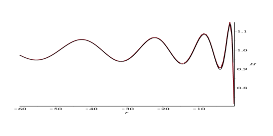
Figure 42: The red and black plots are, respectively, the numeric and large-$r$ asymptotic solutions ($\mathrm{e}^{u(\tau)}=H(r)$, $\tau=r$) of equation (D.1) corresponding to the initial datum $\mathrm{e}^{u(0)}=H(0)=5/7$.

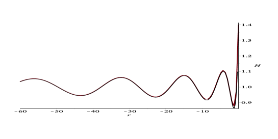
Figure 43: The red and black plots are, respectively, the numeric and large-$r$ asymptotic solutions ($\mathrm{e}^{u(\tau)}=H(r)$, $\tau=r$) of equation (D.1) corresponding to the initial datum $\mathrm{e}^{u(0)}=H(0)=7/5$.

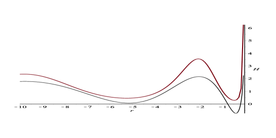
Figure 44: The red and black plots are, respectively, the numeric and large-$r$ asymptotic solutions ($\mathrm{e}^{u(\tau)}=H(r)$, $\tau=r$) of equation (D.1) corresponding to the initial datum $\mathrm{e}^{u(0)}=H(0)=100$.

Remark D.1.

In this appendix, we used the manifold defined in [25]. As mentioned above, two equivalent monodromy manifolds were introduced in [25]. For the case $s=0$, this equivalency is established via the identity mapping, because the monodromy data of these manifolds are denoted by the same letters, namely, $g_{1}$, $g_{2}$, and $g_{3}$, which are used in this appendix. On the other hand, in Section 4, we use the monodromy manifold defined in [26]. Since both monodromy manifolds describe the same set of the solutions of equation (1.6) for $a=0$, they should be equivalent. Strictly speaking, though, the manifold considered in Section 4 contains one more parameter which allows one to find, additionally, asymptotics of the function $\varphi(\tau)$ considered in Appendices B and C (see, also, the integral $I(r)$ in Section 6); however, the quadratic contraction of the manifold in Section 4 enumerates only solutions of equation (1.6) with $a=0$, so that this contraction should be equivalent to the manifold employed in this appendix.

We do not consider the mappings between the manifolds discussed above in the general setting; however, we present the explicit mapping between the manifolds for the case $s=0$, which follows from the comparison of the results of this appendix and Lemma 4.1:

$$s=\tilde{s}=0\qquad\Leftrightarrow\qquad s_{0}^{0}=i,\quad s_{0}^{\infty}s_{1}^{\infty}=-1,$$

$$g_{1}=\tilde{g}_{1},\quad g_{2}=-\tilde{g}_{2},\quad g_{3}=\tilde{g}_{3},$$

which coincides, for $s=\tilde{s}=0$, with the transformation (4.10). $\blacksquare$

Acknowledgements

The authors are grateful to R. Conte for discussions related to the Painlevé Property. A. V. is very grateful to the St. Petersburg Branch of the Steklov Mathematical Institute (POMI) for hospitality during the Summer of 2019, when this work began.

References

- [1] Adamson G. W., Sequence A124647 in The On-Line Encyclopedia of Integer Sequences (2006), published electronically at https://oeis.org/
- [2] Andreev F. V., Kitaev A. V., Connection formulae for asymptotics of the fifth Painlevé transcendent on the imaginary axis: I, Stud. Appl. Math. 145 (2020), no. 3, 397–482.
- [3] Bilman D., Ling L., Miller P. D., Extreme superposition: rogue waves of infinite order and the Painlevé-III hierarchy, Duke Math. J. 169 (2020), no. 4, 671–760.
- [4] Bobenko A. I., Eitner U., Painlevé equations in the differential geometry of surfaces, Lecture Notes in Mathematics, 1753, Springer-Verlag, Berlin, 2000.
- [5] Bottomley H., Sequence A053735 in The On-Line Encyclopedia of Integer Sequences (2000), published electronically at https://oeis.org/
- [6] Bruce J., Wall C. T. C., On the Classification of Cubic Surfaces., J. London Math. Soc. (2) 19 (1979), 245–256.
- [7] Buckingham R. J., Miller P. D., On the algebraic solutions of the Painlevé-III equation, Phys. D 441 (2022), Paper No. 133493, 22 pp.
- [8] Contatto F., Dorigoni D., Instanton solutions from Abelian sinh-Gordon and Tzitzeica vortices, J. Geom. Phys. 98 (2015), 429–445.
- [9] Contatto F., Integrable Abelian vortex-like solitons, Physics Letters B 768 (2017), 23–29.
- [10] Conte R., The Painlevé approach to nonlinear ordinary differential equations, The Painlevé Property: One Century Later, 77–180, CRM Ser. Math. Phys., Springer, New York, 1999.
- [11] Dunajski M., Plansangkate P., Strominger-Yau-Zaslow geometry, affine spheres and Painlevé III, Comm. Math. Phys. 290 (2009), 997–1024.
- [12] Dunajski M., Abelian vortices from sinh-Gordon and Tzitzeica equations, Phys. Lett. B 710 (2012), 236–239.
- [13] Erdélyi A., Magnus W., Oberhettinger F., Tricomi F.G., Higher transcendental functions vol. 1, McGraw-Hill Book Company, Inc., New York-Toronto-London (1953) (based, in part, on notes left by Harry Bateman).
- [14] Erdélyi A., Magnus W., Oberhettinger F., Tricomi F.G., Higher transcendental functions vol. 2, McGraw-Hill Book Company, Inc., New York-Toronto-London (1953) (based, in part, on notes left by Harry Bateman).
- [15] Faddeev D. K.; Sominskij I. S., Sbornik zadach po vysshej algebre. (Russian) [Collection of problems on higher algebra] 3d ed., Gosudarstv. Izdat. Tehn.-Teor. Lit., Moscow-Leningrad, 1952, 308 pp.
- [16] Gamayun O., Iorgov N., Lisovyy O., How instanton combinatorics solves Painlevé VI, V and IIIs, J. Phys. A 46:33 (2013), 335203, 29 pages.
- [17] Gromak V. I., Algebraic solutions of the third Painlevé equation, Dokl. Akad. Nauk BSSR 23 (1979), no. 6, 499–502 (Russian).
- [18] Guest M. A., Its A. R., Lin C.-S., Isomonodromy aspects of the equations of Cecotti and Vafa I. Stokes data, Int. Math. Res. Not. IMRN 2015, no. 22, 11745–11784.
- [19] Guest M. A., Its A. R., Lin C.-S., Isomonodromy aspects of the tt* equations of Cecotti and Vafa II: Riemann-Hilbert Problem, Comm. Math. Phys. 336 (2015), no.1, 337-380.
- [20] Guest M. A., Its A. R., Lin C.-S., Isomonodromy aspects of the tt* equations of Cecotti and Vafa III: Iwasawa factorization and asymptotics, Comm. Math. Phys. 374 (2020), no. 2, 923–973.
- [21] Guest M. A., Its A. R., Lin C.-S., The tt*-Toda equations of type, arXiv preprint arXiv:2302.04597 (2023).
- [22] Hildebrand R., Self-associated three-dimensional cones, Beitr. Algebra Geom. 63 (2022), no. 4, 867–906.
- [23] Ince E. L., Ordinary Differential Equations, Dover Publications, New York, 1944.
- [24] Kimberling C., Sequence A057552 in The On-Line Encyclopedia of Integer Sequences (2000), published electronically at https://oeis.org/
- [25] Kitaev A.V., The method of isomonodromic deformations for the "degenerate” third Painlevé equation. (Russian); Zap. Nauchn. Sem. Leningrad. Otdel. Mat. Inst. Steklov. (LOMI) 161 (1987), 45–53; English translation J. Soviet Math. 46 (1989), no. 5, 2077–2083.
- [26] Kitaev A. V., Vartanian A. H., Connection formulae for asymptotics of solutions of the degenerate third Painlevé equation: I, Inverse Problems 20 (2004), 1165–1206.
- [27] Kitaev A. V., Vartanian A., Connection formulae for asymptotics of solutions of the degenerate third Painlevé equation: II, Inverse Problems 26 (2010), 105010, 58pp.
- [28] Kitaev A. V., Meromorphic Solution of the Degenerate Third Painlevé Equation Vanishing at the Origin, SIGMA 15 (2019), 046, 53pp.
- [29] Kitaev A. V., Vartanian A., Asymptotics of integrals of some functions related to the degenerate third Painlevé equation, J. Math. Sci. (N.Y.) 242 (2019), 715–721.
- [30] Legendre A. M., Théorie des Nombres, Paris: Firmin Didot Frères, 1830.
- [31] Lehmer D. H., A note on trigonometric algebraic numbers, Amer. Math. Monthly 40 (1933), no. 3. 165–166.
- [32] Ohyama Y., Kawamuko H., Sakai H., Okamoto K., Studies on the Painlevé equations. V. Third Painlevé equations of special type and , J. Math. Sci. Univ. Tokyo 13 (2006), 145–204.
- [33] Prasolov V. V., Polynomials, Algorithms and Computation in Mathematics 11, Springer-Verlag, Berlin, 2004.
- [34] Sakamaki Y., Automorphism groups on normal singular cubic surfaces with no parameters, Trans. Amer. Math. Soc. 362 (2010), no. 5, 2641–2666.
- [35] Shimomura S., Series expansions of Painlevé transcendents near the point at infinity. Funkcial. Ekvac. 58 (2015), no. 2, 277–319.
- [36] Shimomura S., Boutroux ansatz for the degenerate third Painlevé transcendents, arXiv preprint arXiv:2207.11495 (2022)
- [37] Sloane N. J. A., Plouffe S., Alford A., Tixier M., Sequences A008615, A008679, A165190, A033182 in The On-Line Encyclopedia of Integer Sequences (2009), published electronically at https://oeis.org/
- [38] Steinmetz N., Nevanlinna theory, normal families, and algebraic differential equations, Universitext, Springer, Cham, 2017.
- [39] Suleimanov B.I., Effect of a small dispersion on self-focusing in a spatially one-dimensional case, JETP Letters 106 (2017), no. 6, 400–405.
- [40] Tracy C. A., Widom H., On exact solutions to the cylindrical Poisson-Boltzmann equation with applications to polyelectrolytes, Phys. A 244.1-4 (1997), 402–413.
- [41] Tracy C. A., Widom H., Asymptotics of a class of solutions to the cylindrical Toda equations, Comm. Math. Phys. 190.3 (1998), 697–721.
- [42] Vartanian A., Trans-series asymptotics of solutions to the degenerate Painlevé III equation: a case study, archive preprint arXiv:2010.11235 (2020).
- [43] Watkins W., Zeitlin J., The minimal polynomial of , Amer. Math. Monthly 100 (1993), no. 5, 471–474.