A simple and efficient route towards improved energetics within the framework of density-corrected density functional theory

Abstract

The crucial step in density-corrected Hartree–Fock density functional theory (DC(HF)-DFT) is to decide whether the density produced by the density functional for a specific calculation is erroneous and hence should be replaced by, in this case, the HF density. We introduce an indicator, based on the difference in non-interacting kinetic energies between DFT and HF calculations, to determine when the HF density is the better option. Our kinetic energy indicator directly compares the self-consistent density of the analysed functional with the HF density, is size-intensive, reliable, and most importantly highly efficient.

Moreover, we present a procedure that makes best use of the computed quantities necessary for DC(HF)-DFT by additionally evaluating a related hybrid functional and, in that way, not only “corrects” the density but also the functional itself; we call that procedure corrected Hartree–Fock density functional theory (C(HF)-DFT).

University of Cambridge] Yusuf Hamied Department of Chemistry, University of Cambridge, Cambridge

1 Introduction

Density functional theory (DFT) is a widely used approach in computational physics and chemistry, owing to the fact that it allows for the relatively simple approximation of many-body effects, providing useful accuracy at low computational cost. Despite the existence of hundreds of density functionals, most DFT calculations use only a few standard functionals, often in the form of (meta) general gradient approximations ((m)GGAs).¹ While (m)GGAs are true Kohn–Sham² (KS) density functionals, consisting of a local multiplicative KS potential, local and semi-local density functionals tend to over-delocalise charge. This over-delocalisation is associated with several well-known problems in density functional theory, including delocalisation error,^{3, 4, 5, 6, 7, 8, 9, 10} one-electron self-interaction error,¹¹ many-electron self-interaction error,^{12, 13, 14} missing derivative discontinuities in the energy as particle numbers pass through integer values — density functionals are too smooth —^{15, 16, 17} and fractional charge and spin errors;^{18, 19, 20} and is the reason for e.g. unbound anions, incorrect molecular dissociation curves, and underestimated reaction barriers.^{5, 21}

To address the problem of over-delocalisation, various approaches have been developed, such as self-interaction corrections,¹¹ the admixture of exact Hartree–Fock^{22, 23, 24} (HF) exchange, the localised orbital scaling correction (LOSC),⁶ and range-separation methods²⁵. Moreover, in cases where standard density functionals fail, using the HF density instead of the self-consistent density, known as HF-DFT, has been shown to improve results significantly.^{26, 27, 28, 29, 30, 31, 32} For a comprehensive benchmark of HF-DFT the interested reader is referred to the work of Martin and co-workers³³.

The good performance of HF-DFT and its appealing theoretical and practical simplicity has led Burke and co-workers to the development of density-corrected (HF) density functional theory (DC(HF)-DFT).^{34, 35, 36, 37, 1, 38, 39, 40, 41, 42, 43} Broadly speaking, this method involves two key steps: assessing whether the density generated by the density functional requires correction or replacement, and then, if necessary, substituting the HF density and evaluating the functional on that density (performing a HF-DFT calculation). This strategy sets DC(HF)-DFT apart from pure HF-DFT, as it ensures — at least in theory — that the HF density is used only when it improves the accuracy of the results. While DC(HF)-DFT has already demonstrated great potential,^{44, 45, 35, 42, 41, 46, 47, 48, 34, 49, 50} in this work we show that further enhancements are possible.

2 Theoretical considerations

2.1 Why density-corrections might be necessary and useful

The exchange-correlation functional is the only part of (KS-)DFT that is not known exactly and hence needs to be approximated. This approximation is then used twice in common DFT calculations, once when determining the density and again when determining the energy of the system; of course, neither is exact. Despite the name, the accuracy of a certain density functional in terms of energetics does not necessarily guarantee the accuracy of the KS potential or the density itself. In fact, most density functional approximations (DFAs) produce poor KS potentials^{51, 52} which can be seen e.g. in the poor orbital energies⁵³ these functionals yield. Nevertheless, in most cases, the density is still very accurate³⁹ because the overall shape of the approximate potential is reasonable, although it is shifted with respect to the exact one, which does not affect the orbitals or the density.^{42, 43}

However, there are large classes of calculations where the density is poor, leading to significant errors in the calculated energies.^{36, 35, 1, 38} Burke and co-workers developed a framework to distinguish such density-driven errors from the errors of the functional itself,¹ the functional errors, by separating the total error according to

$$\Delta\tilde{E}=\underbrace{\tilde{E}[\tilde{n}]-E[\tilde{n}]}_{\Delta\tilde{E}_{\text{xc}}[\tilde{n}]}+\underbrace{E[\tilde{n}]-E[n]}_{D^{\text{ideal}}[\Delta\tilde{n}]}$$ (1)

where exact quantities are denoted without a tilde while approximate quantities are denoted with a tilde symbol; e.g. $E[\tilde{n}]$ denotes the exact functional evaluated on an approximate density. Since it is impractical to evaluate the exact functional on an approximate density, the following separation was proposed:

$$\Delta\tilde{E}=\underbrace{\tilde{E}[\tilde{n}]-\tilde{E}[n]}_{D^{\text{approx}}[\Delta\tilde{n}]}+\underbrace{\tilde{E}[n]-E[n]}_{\Delta E_{\text{F}}}$$ (2)

where the density-driven error ($D^{\text{approx}}$) is now obtained using an approximate functional $\tilde{E}$. If the density-driven error exceeds the functional error ($\Delta E_{\text{F}}$), the calculation is considered abnormal, which means that the functional itself is (or can be) accurate while the produced density, due to a wrong potential, is poor.⁵⁴ For a more detailed discussion of how this is possible and the underlying theory in general, the reader is referred to Ref. 1.

Although highly accurate densities can be computed using coupled cluster or configuration interaction approaches, there are differences in the correlation energy in wave-function theory and density functional theory. Moreover, these high-level wave-function methods produce interacting kinetic energies, while the KS framework requires non-interacting ones. To obtain a corresponding local KS potential and its associated KS orbitals and orbital energies, the density must be inverted, which is computationally expensive and numerically challenging.^{35, 55} However, it has been shown that for abnormal calculations — contrary to normal calculations, where the functional error dominates — the use of the HF density is, in terms of improving the energetics, often not very different from the use of the exact (or highly accurate) density.³⁷ We want to stress that this does not necessarily mean that the HF density is overall better because there is no well-defined meaning of a better density,^{56, 57, 58, 36, 59, 60, 61, 62, 63, 64} as pointed out by Burke and co-workers several times. It simply means that the density functional evaluated on the HF density shows a smaller density-driven error in these cases.³⁷

As previously mentioned, the use of the HF density can be very beneficial; nevertheless, we may not always want to use the HF density. First of all, self-consistency makes the evaluation of properties depending on the derivative of the energy much easier to calculate since a lot of terms vanish. However, we note that a scheme of calculating gradients for HF-DFT was put forward by Bartlett and co-workers.³² Moreover, for normal cases, the self-consistent density usually yields more accurate energetics.³⁹ And finally, the HF density should not be employed if it is spin-contaminated since it should no longer be considered more accurate, as pointed out by Burke and co-workers.⁶⁵

2.2 When to correct the density

Recently, there has been a vigorous discussion about how to evaluate the accuracy of densities.^{56, 57, 58, 36, 59, 60, 61, 62, 63, 64} The problem with this is that the density is a function³⁶, meaning that there are infinitely many numbers to compare and hence many ways to do so. Burke and co-workers argued³⁶ that the energy is the most meaningful measure since it is the quantity that really matters and it is further able to detect even the tiniest differences in the density when they matter, leading to the development of density functional analysis.³⁷ The present work deals with more pragmatic, but related, questions: When is the HF density likely to improve the results obtained with a certain density functional? And how can we decide that efficiently?

In order to detect abnormal calculations, Burke and co-workers put forward a simple heuristic called the density sensitivity defined as³⁷

$$\tilde{S}=\lvert\tilde{E}[n^{\text{LDA}}]-\tilde{E}[n^{\text{HF}}]\rvert$$ (3)

where $n^{\text{LDA}}$ and $n^{\text{HF}}$ denote the LDA and the HF density, respectively. Note that Eq. 3 represents the density sensitivity of one calculation, but the density sensitivity is usually evaluated for the whole reaction of interest. If the density sensitivity of this reaction is above a certain threshold (2 kcal/mol is the usual choice³⁶) the reaction is considered density sensitive and the HF density is employed instead of the self-consistent density to evaluate the reaction energy.

Comparing Eq. 3 with Eq. 1 it becomes apparent that this measure resembles the exact one if the curvature of the approximate functional is accurate,¹ the LDA density is close to the self-consistent density of the functional under investigation (denoted by $\tilde{E}$), and the HF density is close to the exact one. These conditions are, of course, rarely met, but this is not very problematic since we are only interested in answering the question whether the energy calculation is sensitive with respect to the density in use or not. However, there are some weaknesses of the proposed density sensitivity measure, especially in combination with DC(HF)-DFT:

First of all, the density sensitivity is independent of the density generated by the functional being analysed, although it can differ significantly from the LDA one. Furthermore, when the density sensitivity exceeds a specified threshold, the HF density is presumed to be a better choice than the self-consistent density, or even an accurate approximation of the exact density.⁴¹ This assumption, coupled with the utilization of the LDA density, rather than the functional’s self-consistent density, introduces potential difficulties.

Moreover, the density sensitivity is size extensive, which necessitates adjustment of the threshold according to the system size.^{40, 34} Additionally, when calculating small energy values such as torsional barrier heights or non-covalent interactions, the threshold must be further adapted,^{65, 34} which can introduce an element of arbitrariness.

As mentioned above, the density sensitivity could, in principle, be applied to single calculations, but it is typically used for reaction energies. While it is, of course, true that key chemical concepts are determined by energy differences and that absolute energies are not even observables,⁶⁶ this introduces a source of error cancellation.¹ There is a further source of error cancellation in the density sensitivity measure: since the density sensitivity is measured using an approximate exchange-correlation functional, errors in that functional can cancel the ones in the density as functional errors and density-driven errors have opposite signs.⁴² That such an error cancellation can occur is well known.^{67, 55, 29}

In that context, we also mention the work of Kepp, who proposed a recipe to assess the degree of normality which evaluates four distinct functionals on each other’s self-consistent densities.⁶⁶ The use of various functionals reduces the probability of error cancellation in measuring the abnormality of the reaction. However, the HF density was not included in this measure, preventing it from detecting a lot of abnormalities. Additionally, for a trial set of $N$ functionals, $N^{2}$ calculations are necessary for each system, which is computationally demanding.

This leads us to a final issue: the value of DFT lies in its computational efficiency, and this would be significantly reduced if additional HF calculations had to be performed every time. Since the majority of calculations are not density sensitive⁶⁵, this is a weakness needing to be addressed in order to facilitate more widespread use of DC(HF)-DFT.

In the subsequent discussion, we will try to address the aforementioned weaknesses of the density sensitivity by proposing a novel simple and efficient heuristic approach based on the non-interacting kinetic energy for detecting abnormal DFT calculations.

3 The kinetic energy indicator

3.1 Theoretical rationalisation

To begin with, let us summarise the key features that an indicator should possess in order to signal the superiority of the HF density for a given DFT calculation, as these characteristics serve as the foundation for our kinetic energy indicator:

First, the indicator should compare, using a specified metric, the self-consistent density of the specific functional with the HF density. Second, it should be size-intensive; so, no adjustment of thresholds should be necessary. Third, it should avoid error cancellation as much as possible. Fourth, it should be efficient.

Our proposed kinetic energy indicator is very simple and requires two calculations: a converged DFT calculation using our preferred density functional and a converged HF calculation on the very same system; it then compares the two (non-interacting) kinetic energies. If the HF kinetic energy is larger than the one obtained from the DFT calculation, the HF density is the better choice. But how did we arrive at that conclusion?

We first appeal to the textbook example of a particle in a 1-dimensional box with potential $V(\mathbf{r})=0$. Since we set the potential to 0, the energy of the particle is given by⁶⁸

$$E=T=\frac{\pi^{2}}{2L^{2}}$$ (4)

with $L$ denoting the length of the box. As is obvious, the total energy — and hence the kinetic energy — becomes smaller the larger the box gets. Transferring the conclusion from this extremely simplified example to the problem of delocalisation, we would expect a similar behaviour: a decrease in the kinetic energy if the system delocalises.

To illustrate the lowering of the kinetic energy with increasing delocalisation, we calculated the energies of the H atom using different functionals of the form

$$E=T_{\text{s}}+E_{\text{en}}+E_{\text{J}}+(1-a)E^{\text{PBE}}_{\text{xc}}+aE^{\text{HF}}_{\text{x}}+E_{\text{nn}}$$ (5)

where we vary the value of the mixing factor $a$ from 0 to 1. In Eq. 5, $T_{\text{s}}$ denotes the non-interacting kinetic energy, $E_{\text{en}}$ denotes the energy stemming from the attraction of the electrons to the nuclei, $E_{\text{J}}$ denotes the so-called Coulomb energy, $E^{\text{PBE}}_{\text{xc}}$ denotes the PBE^{69, 70} exchange-correlation (xc) energy, and $E^{\text{HF}}_{\text{x}}$ denotes the HF exchange energy. Note that we scale the complete PBE xc-energy and so the PBE0^{71, 72} functional is not within the set of functionals, but we recover the standard PBE functional for $a=0$ and the HF functional for $a=1$.

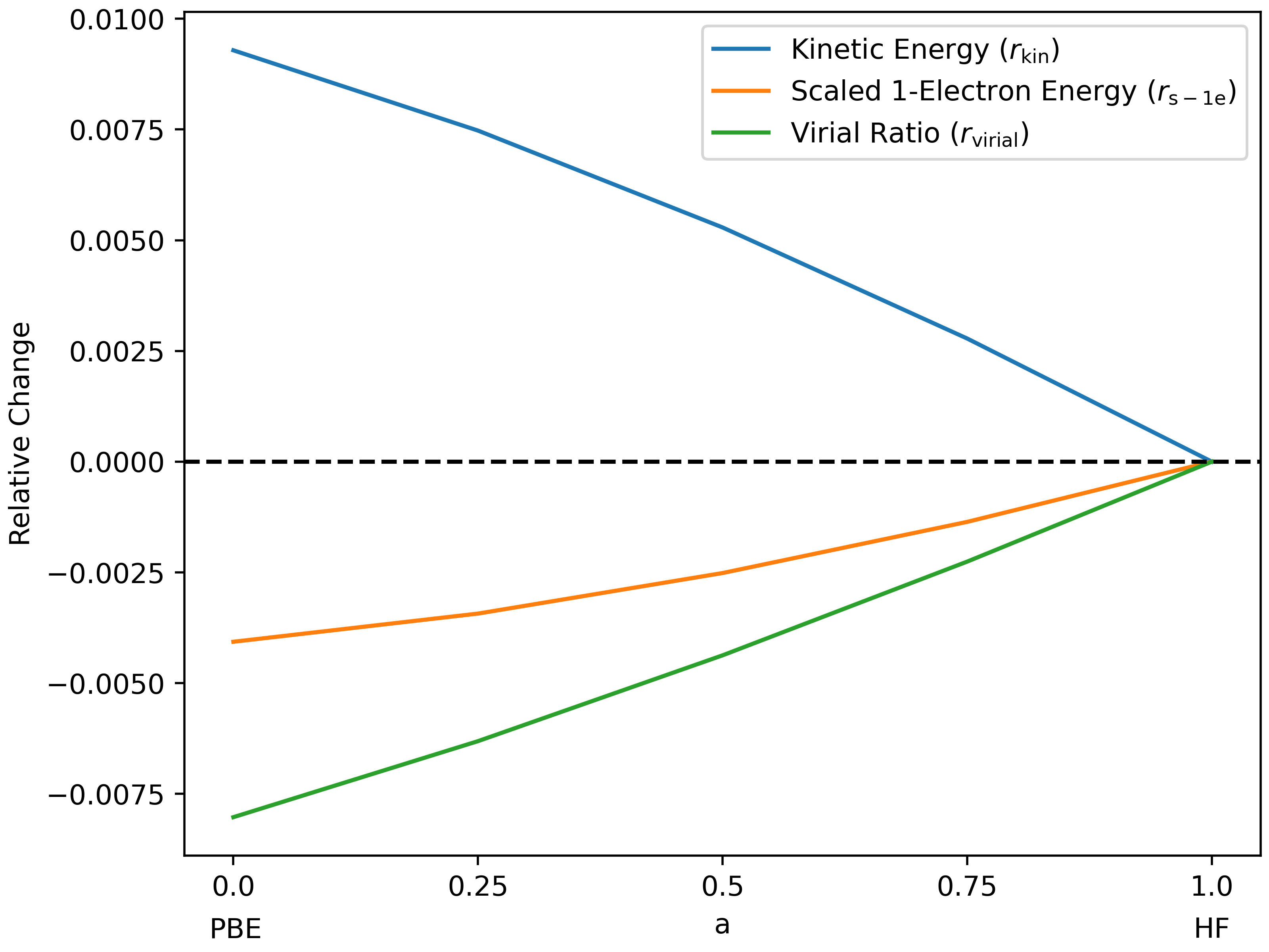
Figure 1: Behaviour of the two indicators and the virial ratio difference when interpolating between pure PBE and pure HF (exact) for the H atom. Note that both the exchange and the correlation part of the PBE functional are scaled and hence the functional obtained for mixing factor $0.25$ does not correspond to the PBE0 functional.

The relative change of the kinetic energy is given by

$$r_{\text{kin}}=\frac{T^{\text{HF}}_{\text{s}}-T^{\text{KS}}_{\text{s}}}{T^{\text{KS}}_{\text{s}}},$$ (6)

and is plotted in Fig. 1. As can be seen, $r_{\text{kin}}$ becomes more and more positive as we move from HF ($a=1$; exact, no delocalisation error) to PBE ($a=0$; delocalisation error), meaning that the kinetic energy obtained using the density functional decreases compared to the HF kinetic energy. As reported by Mezei et al., HF can yield quite erroneous densities but with good gradients and Laplacians.⁵⁶ We therefore consider another indicator, the scaled one-electron energy indicator, to avoid biasing towards derivatives. The scaled one-electron energy indicator is given by

$$r_{\text{s-1e}}=\frac{E^{\text{HF}}_{\text{en}}-E^{\text{KS}}_{\text{en}}}{E^{\text{KS}}_{\text{en}}}-\frac{T^{\text{HF}}_{\text{s}}-T^{\text{KS}}_{\text{s}}}{T^{\text{KS}}_{\text{s}}}$$ (7)

The idea behind the scaling is to put an equal weight on the density itself and its derivatives. This time, the calculation is considered abnormal if $r_{\text{s-1e}}$ becomes negative. As can be seen, the scaled one-electron indicator leads to the same conclusions for this simple example.

The virial theorem in KS-DFT is given by^{73, 74}

$$\gamma[n]=\frac{V^{\text{KS}}[n]-T_{\text{c}}[n]}{T^{\text{KS}}_{\text{s}}[n]+T_{\text{c}}[n]}=-2.0$$ (8)

In Fig. 1 we further show another quantity, which is the change in the virial ratio given by

$$r_{\text{virial}}=\lvert\gamma^{\prime}[n^{\text{HF}}]+2.0\rvert-\lvert\gamma^{\prime}[n^{\text{DFT}}]+2.0\rvert$$ (9)

with the virial ratio defined as

$$\gamma^{\prime}[n] =\frac{V^{\text{KS}}[n]}{T^{\text{KS}}_{\text{s}}[n]}$$ (10)

$$V^{\text{KS}}[n] =E_{\text{en}}+E_{\text{J}}+E_{\text{xc}}+E_{\text{nn}}$$ (11)

As can be seen in Eq. 9, $r_{\text{virial}}$ is negative if the virial ratio (Eq. 10) evaluated on the HF density is closer to the value of $-2.0$ than the virial ratio evaluated on the self-consistent density. We should highlight a few things here: First, when comparing Eq. 10 and Eq. 8, it is clear that the virial ratio $\gamma^{\prime}$ should not be expected to be exactly $-2.0$ — due to the fact that the correlation part of the kinetic energy $T_{\text{c}}$ is (should be) included in the exchange-correlation energy — but it is usually quite close. Second, as can be seen in Fig. 1, $r_{\text{virial}}$ could, in principle, serve as an indicator. However, since the virial ratio only holds in the complete basis set limit and for atoms or molecules in their equilibrium geometry, we have chosen not to pursue it. Additionally, by inspecting Eq. 8 it could be expected that the virial ratio gets closer to $-2.0$ with increasing $T^{\text{KS}}_{\text{s}}$ (and decreasing $T_{\text{c}}$). Third, inspecting Eq. 8 or 10 and considering that $V^{\text{KS}}$ includes, in contrast to the HF functional, an energy contribution stemming from electron correlation, it could be assumed that $T^{\text{KS}}_{\text{s}}$ should be larger than its HF counterpart. We note that this “contraction effect of correlation” was also reported by Baerends and co-workers,⁷⁵ who found that $T_{\text{s}}^{\text{KS}}>T_{\text{s}}^{\text{HF}}$ holds true for all of their investigated cases. In this context it should be noted that although the definition in terms of orbitals is identical, the HF and the KS non-interacting kinetic energies are different,⁷⁶ since the HF method minimises the expectation value of the Hamiltonian over all Slater determinants while the KS Slater determinant can only be constructed from orbitals stemming from a local multiplicative potential yielding the exact density according to

$$\rho(\mathbf{r})=\sum_{i}\lvert\phi^{\text{KS}}_{i}(\mathbf{r})\rvert^{2}$$ (12)

However, that difference was shown to be small and this is why it is neglected in DC(HF)-DFT.³⁵ It is also true that, contrary to the KS case, no universal proof exists that the HF kinetic energy needs to be smaller than (or equal to) the exact (interacting) kinetic energy; or in other words, that $T_{\text{c}}$ needs to be non-negative. However, a realistic counter example has not been found.⁷⁷

3.2 Sanity checks on typical normal and abnormal calculations

To test the kinetic energy indicator, we evaluated it for various DFT calculations on the different systems contained in the S22^{78, 79} and B30^{80, 81} test sets, serving as examples for normal and abnormal calculations, respectively.³⁷ Both test sets were developed to assess the accuracy of a method in calculating non-covalent interaction energies between molecules and complexes, with high-level coupled-cluster calculations serving as a reference. The well-established S22 test set was designed to represent non-covalent interactions in biological molecules in a balanced way (hydrogen bonds, weak dispersion bonds, and mixed scenarios). On the other hand, the B30 test set contains non-covalent interactions that showed to be challenging for especially pure density functionals: halogen bonds, chalcogen bonds, and pnicogen bonds.⁸⁰ With “systems” we thus mean the various complexes/dimers plus the respective sub-systems/monomers.

We used several functionals for our tests: the LDA^{82, 83, 84} functional as an example known for large delocalisation errors; the PBE^{69, 70} and the SCAN^{85, 86} functionals since they are probably the most popular non-empirical functionals in use today and SCAN additionally fulfills many exact constraints; and the M06-L^{87, 88} functional as an example for a highly empirical functional.

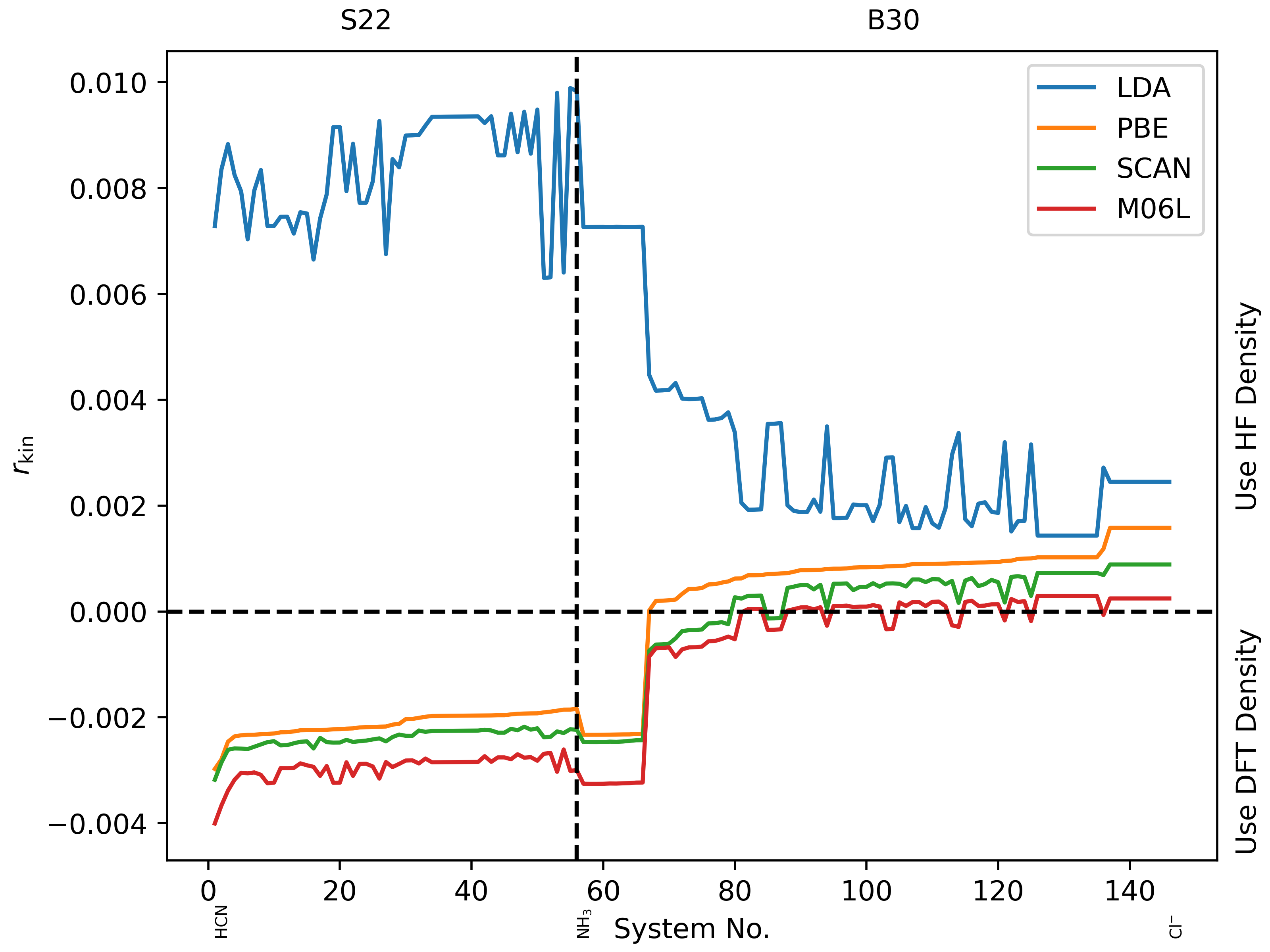
Figure 2: Relative change of the kinetic energy ($r_{\text{kin}}$) for different DFT calculations on the S22 and B30 test sets.

Fig. 2 shows $r_{\text{kin}}$ as defined above for the different functionals and systems in the S22 and B30 test sets. Note that all systems of a specific test set in this section were ordered by increasing value of $r_{\text{kin}}$ obtained with the PBE functional; the complete ordered lists can be found in the supporting information. As can be seen, for LDA the indicator is always larger than $0$ and hence always suggests the use of the HF density. For the other three functionals (PBE, SCAN, and M06-L) all calculations in the S22 test set are predicted to be normal, whereas most of the calculations contained in the B30 test set are predicted to be abnormal. Since we chose the B30 test set to represent abnormal DFT calculations, these observations coincide exactly with our expectations. Also note how the indicator changes for different functionals: based on this indicator, the LDA density performs worse, followed by PBE, SCAN, and finally M06-L. Furthermore, the three (m)GGAs seem to produce quite similar densities according to our indicator. While this is interesting to observe, we stress that our indicator is not intended to assess the quality of the different densities but only to predict if the HF density is a better choice for a specific calculation.

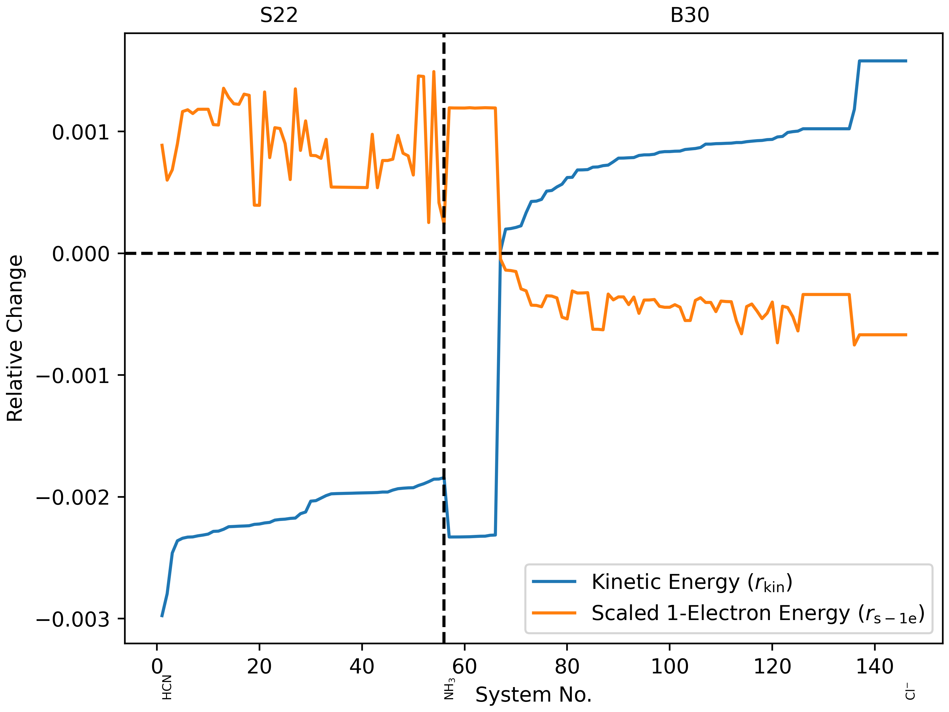
Figure 3: Relative change of the kinetic energy ($r_{\text{kin}}$) and the scaled one-electron energy ($r_{\text{s-1e}}$) for the PBE functional on the S22 and B30 test sets.

In Fig. 3 we additionally show $r_{\text{kin}}$ together with $r_{\text{s-1e}}$ for the PBE functional. As can be seen, as for the H atom, the kinetic energy indicator and the scaled one-electron indicator lead to the same conclusions (recall that abnormal calculations lead to negative values for $r_{\text{s-1e}}$) and hence we will only use the kinetic energy indicator in the following discussions.

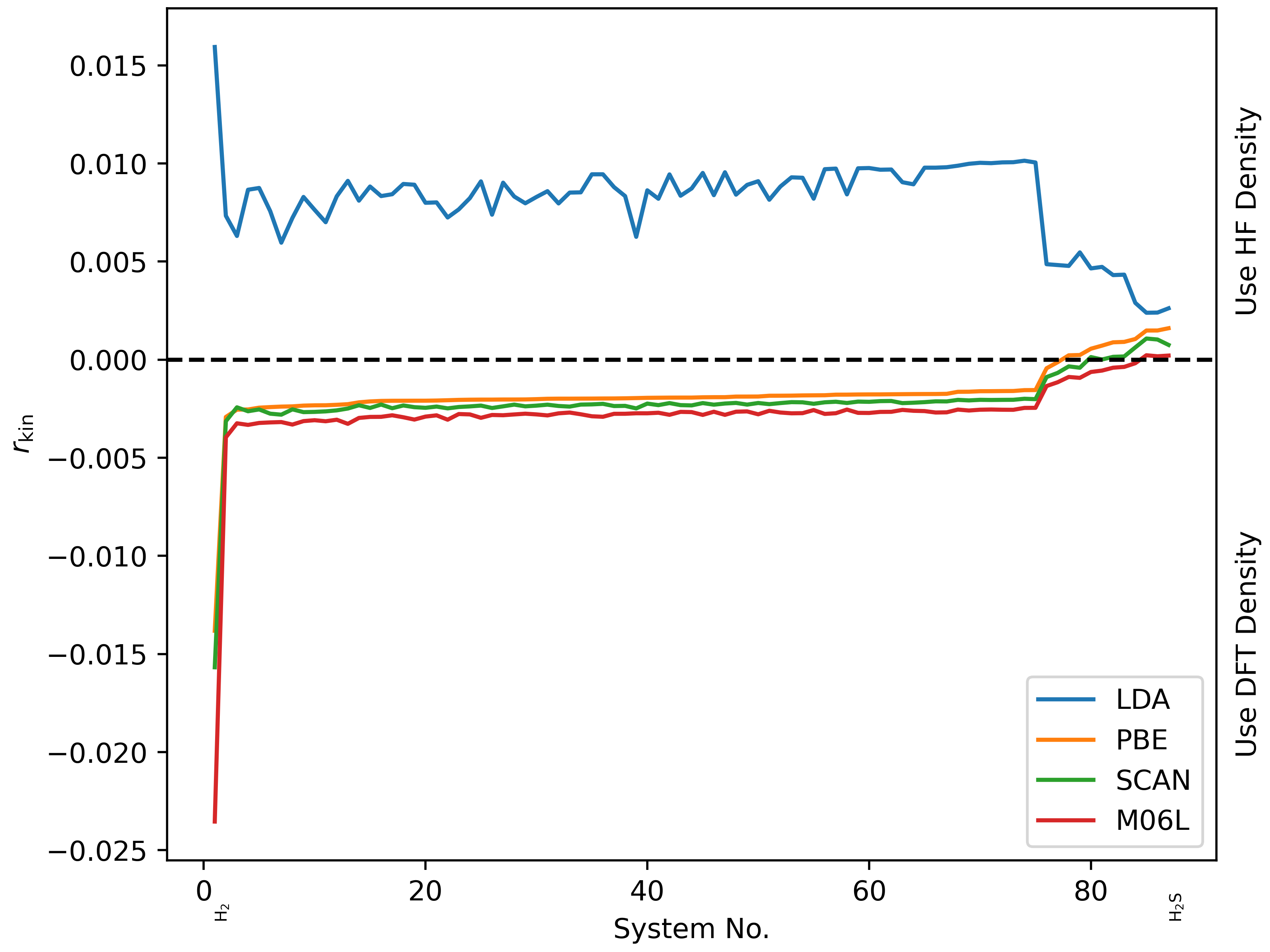
Figure 4: Relative change of the kinetic energy ($r_{\text{kin}}$) for different DFT calculations on the FH51 test set. Due to convergence problems for some systems, the cc-pVQZ^{89, 90, 91, 92} basis set was used for the SCAN functional.

We performed further sanity checks on a test set we would expect to include mostly normal calculations: the FH51 test set⁹³ consisting of reaction energies in small inorganic and organic systems. The results are shown in Fig. 4.

As can be seen, the results are in line with our expectations: in case of LDA the HF density should always be the better choice, while the densities produced by the other three functionals should be perfectly normal in the vast majority of cases.

We mentioned before that one of the characteristics an indicator should have in our opinion is to avoid error cancellation as much as possible. The two main sources of error cancellation as mentioned above are the use of an approximate exchange-correlation functional to decide whether the HF density should be used or not and further considering whole reactions instead of single calculations. Although, of course, there is the virial ratio connecting $V^{\text{KS}}$ and $T_{\text{s}}$, we are convinced that using the (non-interacting) kinetic energy functional — which is exactly given in terms of orbitals — is a step in the right direction when it comes to avoiding the first source of error cancellation. Addressing the second source of error cancellation is simple: we consider a reaction abnormal — and hence perform all necessary calculations using the HF density — if one of the calculations is abnormal.

In the following, we will assess how well this procedure works by benchmarking the accuracies of the resulting DC(HF)-DFT methods for different test sets taken from the GMTKN55 database.⁹⁴

3.3 Performance

Let us start with the performance for the non-covalent interaction energies contained in the S22 and the B30 test sets. In the last section, it was shown that the kinetic energy indicator always suggests the use of the HF density for LDA. As can be seen in Table 1, this leads to a significant lowering of the mean absolute error (MAE) for both test sets. That the HF density performs better than the LDA density is in line with observations presented in related works.^{59, 56} For the other three functionals the conclusion is the same: the kinetic energy indicator suggests the “more accurate” density in both cases; the self-consistent one for the S22 and the HF one for the B30 test set.

We further tested our kinetic energy indicator for the chemical problems included in the FH51, the G21EA^{95, 96, 94} (adiabatic electron affinities), and the DARC^{96, 94, 97} (Diels-Alder reactions) test sets. Overall, the kinetic energy indicator behaves as desired and leads to significant improvements when the DFT densities are erroneous.

Table 1: Mean absolute errors in kcal/mol of different functionals for different test sets.

	S22	B30	FH51a	G21EA	DARC
LDA	2.18	8.26	6.69	7.83	11.83
LDA@HF	1.35	5.02	5.44	6.92	8.86
DC(HF)-LDA	1.35	5.02	5.44	6.73	8.86
PBE	2.56	2.46	3.44	3.69	6.63
PBE@HF	3.26	1.00	3.44	2.93	7.64
DC(HF)-PBE	2.56	1.00	3.55	3.04	6.63
SCAN	1.16	2.48	2.99	3.37	2.89
SCAN@HF	1.54	0.77	2.56	4.20	3.41
DC(HF)-SCAN	1.16	0.78	2.96	3.29	2.89
M06-L	0.72	1.34	2.84	3.46	8.15
M06-L@HF	0.85	0.77	2.07	4.13	5.39
DC(HF)-M06-L	0.72	0.86	2.81	3.48	8.15

^a Due to convergence problems for some systems, the cc-pVQZ^{89, 90, 91, 92} basis set was used for the SCAN functional.

However, questions about the reliability of our indicator arise when evaluating the DARC test set using the M06-L functional. In this case, the kinetic energy indicator clearly favours the “less accurate” density. We conducted further examination to understand this behaviour better.

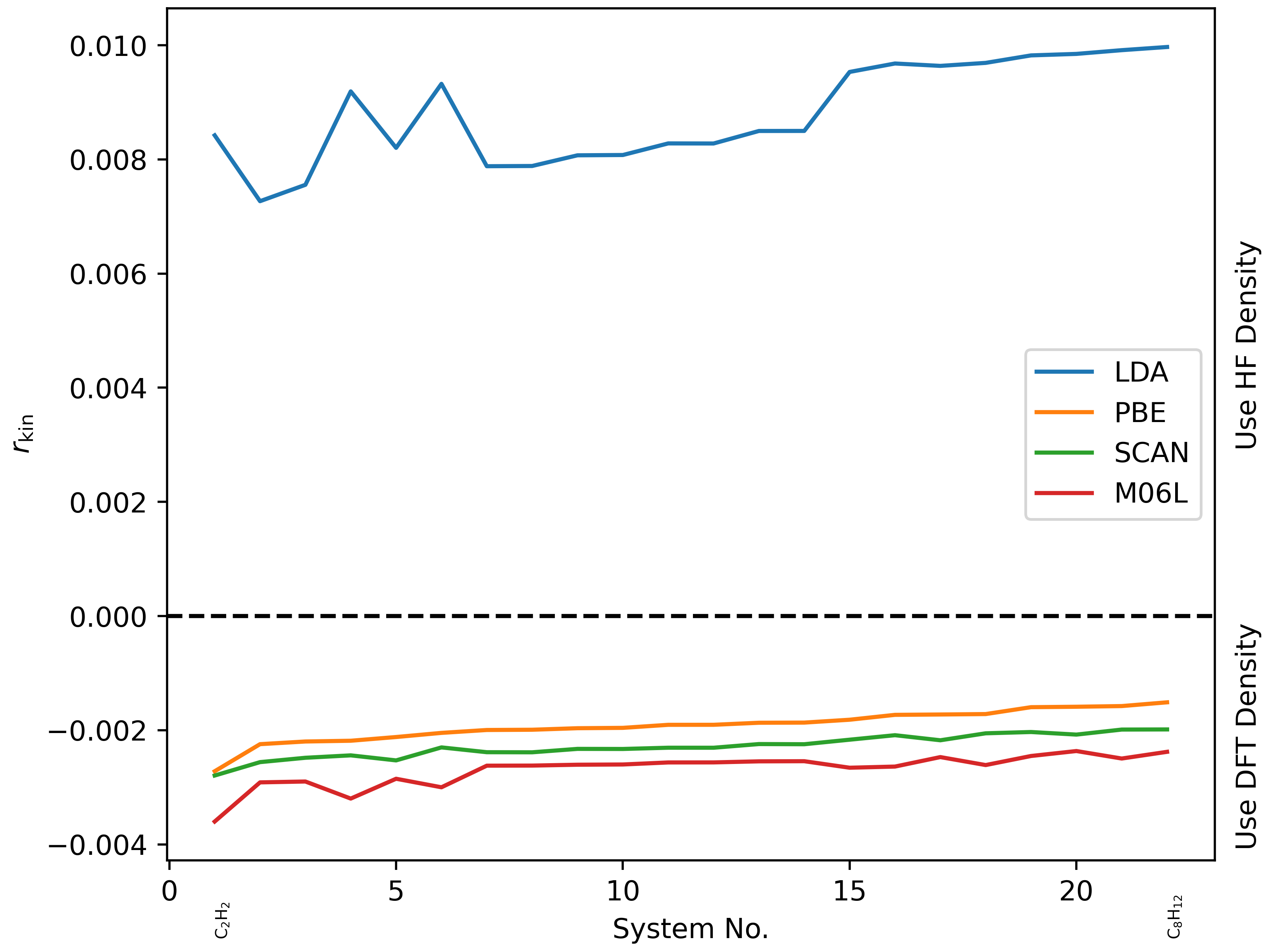
Figure 5: Relative change of the kinetic energy ($r_{\text{kin}}$) for different DFT calculations on the DARC test set.

Fig. 5 shows $r_{\text{kin}}$ for the calculations in the DARC test set performed with the LDA, PBE, SCAN, and M06-L functionals. As can be seen, only for the LDA functional the kinetic energy indicator suggests the use of the HF density. Furthermore, as for the examples presented in the last section, the densities produced by the different (m)GGAs seem to be quite similar (at least according to our kinetic energy indicator). Also note that the kinetic energy indicator performs very well for all functionals except M06-L. Therefore, we tested how the SCAN functional — performing best on the DARC test set — performs when evaluated on the M06-L density. The results are shown in Fig. 6.

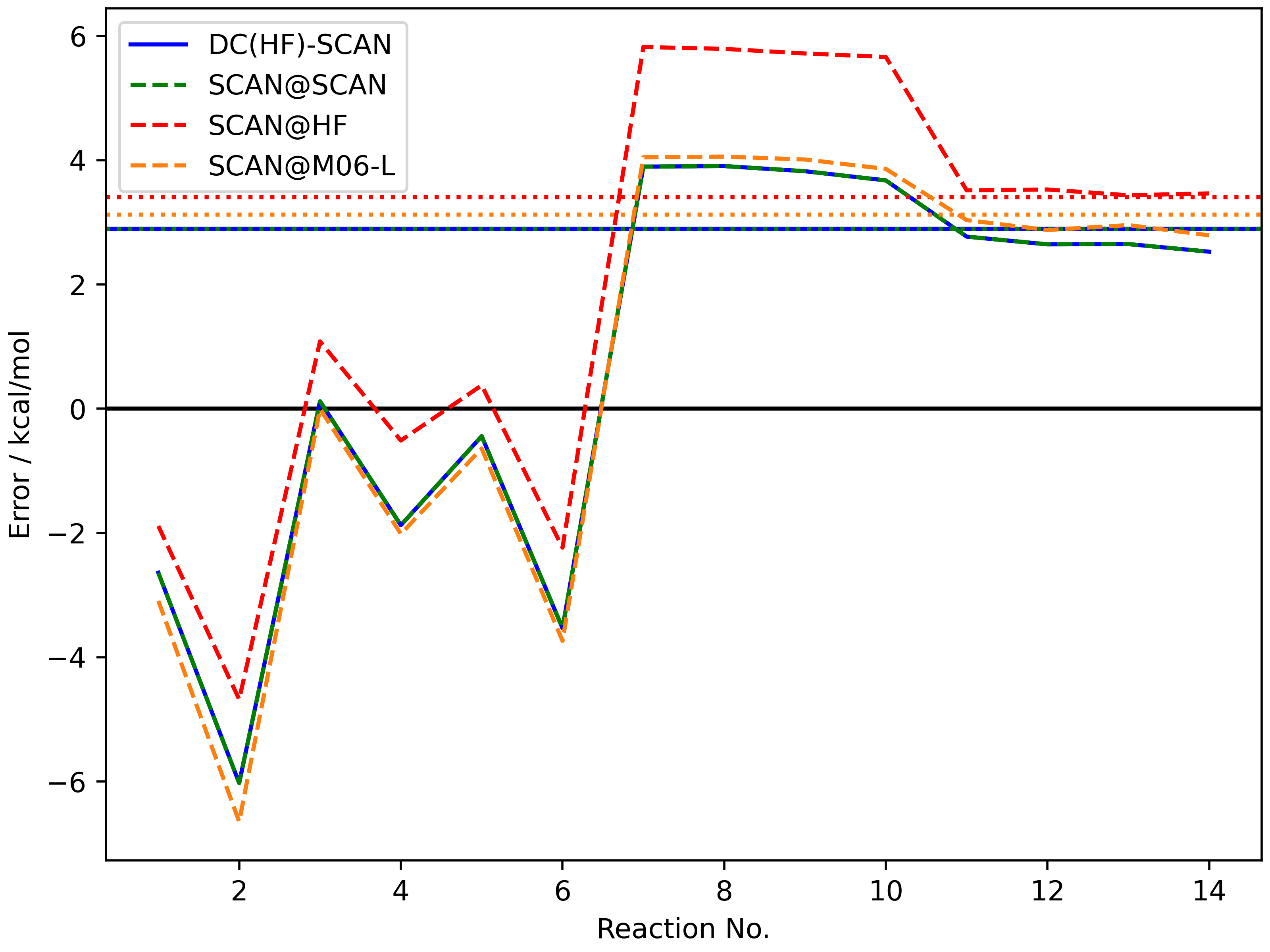
Figure 6: Errors in kcal/mol for the different reactions contained in the DARC test set using the SCAN functional on different densities. The coloured horizontal lines show the respective mean absolute errors.

As can be seen, the errors of the SCAN functional evaluated on its self-consistent density and on the M06-L density are indeed very similar and hence the kinetic energy indicator correctly predicts the M06-L density to be normal — if the SCAN density is normal then the M06-L density should be normal as well. Therefore, the better performance of M06-L@HF is probably due to a fortuitous cancellation of the functional error and the errors in the HF density. Although this behaviour of our kinetic energy indicator leads to worse results in this case, it is still encouraging that it is able to make this distinction. We assume similar reasons for the slight worsening of the PBE results for the FH51 test set.

3.4 Efficiency

As mentioned before, another key feature a good indicator should possess is efficiency. So far, our kinetic energy indicator does not seem to improve a lot upon the density sensitivity put forward by Burke and co-workers in this respect. In order to address this, we propose the following procedure:

First, converge the DFT calculation. Second, use the converged DFT density as initial guess for a HF calculation. Third, evaluate one Fock matrix and update the orbitals and density. Fourth, evaluate the kinetic energy using the updated orbitals and compare it with the converged DFT kinetic energy. Fifth, only converge the HF calculation if $T_{\text{s}}^{\text{HF, 1-iter}}>T_{\text{s}}^{\text{KS}}$.

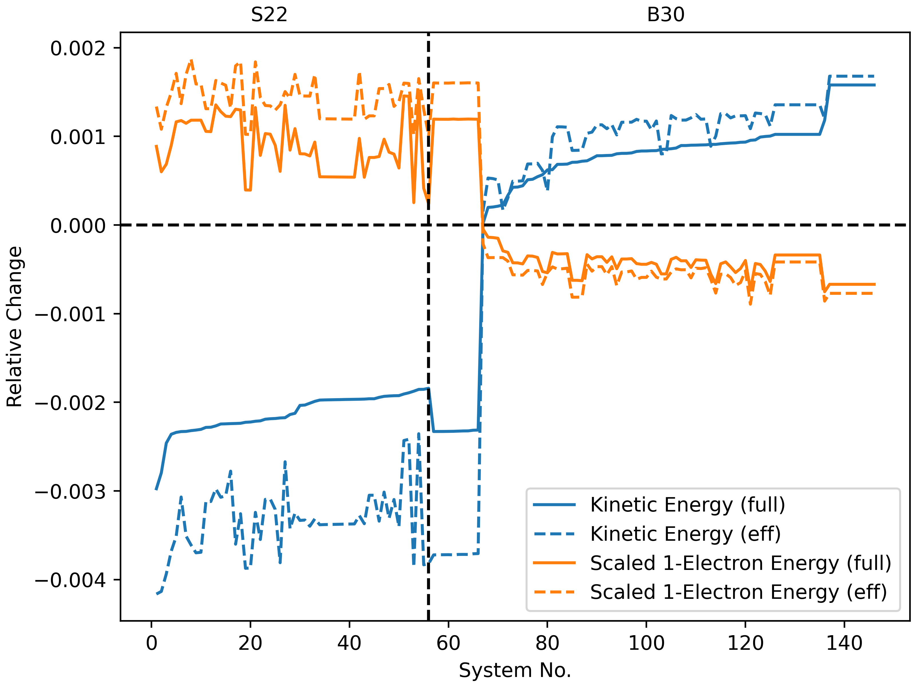
Figure 7: Comparison of the two indicators evaluated with unconverged HF orbitals (only one HF iteration; eff) with their converged counterparts (full).

We investigated that scheme for the S22 and the B30 test sets using the PBE functional. The indicators $r_{\text{kin}}$ and $r_{\text{s-1e}}$ after only one HF iteration (denoted with “eff”) and the converged counterparts (denoted with “full”) are shown in Fig. 7. As can be seen, the indicators after only one HF iteration lead to the same results. Moreover, the unconverged indicators tend to be larger in magnitude, which is ideal since it ensures correct predictions.

Figure 8: Cumulative timings for the S22, B30, and FH51 test sets.

Fig. 8 shows cumulative timings of pure LDA and PBE, as well as full DC(HF)-PBE (converging the HF calculation to assess whether the HF or the self-consistent density should be used) and efficient DC(HF)-PBE (only one iteration of HF for the assessment) for the S22, B30, and FH51 test sets; additionally, the time needed for all test sets together is shown. The reason why we also show LDA timings is the fact that the LDA as well the HF density are needed to evaluate the density sensitivity according to Eq. 3.

To start with, we note that the HF calculations are significantly more expensive than both the LDA and the PBE calculations; in fact, the difference between LDA and PBE is negligible. Second, the savings in terms of computational cost are enormous when our efficient DC(HF)-PBE method is employed, and, of course, get even larger the more normal calculations are included. We want to stress again that the vast majority of DFT calculations is normal and hence our proposed procedure is an important step to make the use of DC(HF)-DFT more routine.

Finally, although it was not necessary in the cases investigated here, it should be noted that, if the efficient indicator suggests the use of the HF density, it is, of course, possible and probably also advisable to check the indicator again after the HF calculation is fully converged; there is no disadvantage in doing that. Additionally, the density sensitivity could be evaluated with a small extra cost to introduce a further control mechanism. In that way, the density sensitivity and the kinetic energy indicator can be considered complementary.

3.5 Beyond density corrections

In the last section, we proposed a scheme that significantly improves the efficiency of our kinetic energy indicator. In this section, we want to go one step further: since our indicator necessitates one iteration of HF in any case, it naturally lends itself to including exact (HF) exchange in the final energy and, in that way, additionally “correcting” the functional. Consider the PBE functional as an example:

First, we converge a PBE calculation. After that, we use the PBE density to evaluate the Fock matrix, update the orbitals, and compare the updated kinetic energy with the one obtained using the PBE functional. If the PBE kinetic energy is larger, we already have everything we need to evaluate the PBE0 functional on the PBE density. If the updated kinetic energy is larger, we converge the HF calculation and the only thing we need to do now is to evaluate the PBE exchange-correlation potential using the HF density on top of that, which is, as can be seen in Fig. 8, almost negligible in terms of computational cost. We note that the choice which hybrid to evaluate in this step is completely flexible. Instead of DC(HF)-DFT we call this procedure C(HF)-DFT (“corrected” instead of “density corrected”), or for the specific case of PBE, C(HF)-PBE.

Table 2: Mean absolute errors in kcal/mol of different functionals for different test sets.

	S22	B30	FH51	G21EA	DARC
PBE	2.56	2.46	3.44	3.69	6.63
DC(HF)-PBE	2.56	1.00	3.55	3.04	6.63
C(HF)-PBE	2.41	0.90	2.62	2.59	3.08
PBE0	2.38	1.62	2.63	2.53	3.05

We tested the proposed method on the test sets already used above. The results are shown in Table 2. As can be seen, C(HF)-PBE significantly improves upon pure PBE and performs similarly to full (pure) PBE0. It is also worth noting the improvement of C(HF)-PBE compared to PBE0 for the B30 test set, which is due to the use of the HF density in that case.

4 Computational details

All calculations were carried out using a development version of the FermiONs++ programme package developed in the Ochsenfeld group.^{98, 99, 100} The binary has been compiled with the GNU Compiler Collection (GCC) version 12.1. The calculations were executed on a compute node containing 2 Intel Xeon E5-2630 v4 CPUs (20 cores / 40 threads; 2.20 GHz). All runtimes given are wall times, not CPU times.

The evaluations of the exchange-correlation terms were performed using the multi-grids defined in Ref. 101 (smaller grid within the SCF optimization and larger grid for the final energy evaluation), generated with the modified Becke weighting scheme.¹⁰¹ The SCF convergence threshold was set to $10^{-6}$ for the norm of the difference density matrix $||\Delta\mathbf{P}||$.

We employ the integral-direct resolution-of-the-identity Coulomb (RI-J) method of Kussmann et al.¹⁰² for the evaluation of the Coulomb matrices and the linear-scaling semi-numerical exact exchange (sn-LinK) method of Laqua et al.¹⁰³ for the evaluation of the exact exchange matrices.

For the calculations on the H atom, the def2-QZVPPD^{104, 105, 106} basis set together with the def2-universal-JFIT¹⁰⁷ auxiliary basis set was employed. If not stated otherwise, all calculations included in the test sets S22, B30, FH51, G21EA, and DARC were performed using the aug-cc-pVQZ^{89, 108, 90, 91, 92} basis set in combination with the cc-pVTZ-JKFIT¹⁰⁹ auxiliary basis set.

5 Conclusion

In conclusion, we presented a simple yet efficient procedure to perform DC(HF)-DFT calculations. In this procedure, the crucial step of deciding whether the self-consistent or the HF density should be used to evaluate the density functional is conducted employing a simple heuristic based on the difference between the non-interacting kinetic energies obtained from the analysed functional and the HF method, called the kinetic energy indicator. Our kinetic energy indicator offers several key characteristics that make it stand out from other methods: Firstly, it directly compares the self-consistent density of the analysed functional with the HF density. Secondly, it is size-intensive, meaning that it is suitable for use in both large and small systems. Thirdly, it reduces the probability of error cancellation, making it more reliable. Finally, it is highly efficient. We further note that our kinetic energy indicator is extremely simple to apply in a retrospective analysis of DFT calculations, assuming that the non-interacting kinetic energies of the analysed DFT calculations are known. All that is necessary is to converge a HF calculation and compare the two non-interacting kinetic energies.

It was shown that the kinetic energy indicator reliably detects calculations where the use of the HF density leads to improved results. Furthermore, the high efficiency of our indicator was demonstrated on three different test sets contained in the GMTKN55 database.

In addition, we have introduced a new procedure, called C(HF)-DFT, which not only corrects the density if necessary, but also “corrects” the functional by evaluating a related hybrid at almost no extra computational cost. We have demonstrated its effectiveness using the PBE functional, showing a significant improvement in accuracy that is comparable to that of its parent hybrid, PBE0. Additionally, if the parent hybrid suffers from a density-driven error, C(HF)-DFT can achieve even higher accuracy. Extending this procedure to double-hybrids is work in progress.

Overall, our presented methods provide simple and effective solutions for improving density functional evaluations. As Burke and co-workers have noted,⁶⁷ even small improvements in our current density functional approximations can have a significant impact on applications in science and technology. Therefore, we hope that our contributions will lead to more widespread application of DC(HF)-DFT and C(HF)-DFT, and, in that way, have a positive impact on quantum chemical applications of all kinds.

D. G. acknowledges funding by the Deutsche Forschungsgemeinschaft (DFG, German Research Foundation) – 498448112. D. G. thanks J. Kussmann (LMU Munich) for providing a development version of the FermiONs++ programme package.

The following files are available free of charge:

• lists_of_energy_contributions.xlsx: Excel file containing all relevant energy contributions for all systems and functionals considered in this work

• ordered_lists_of_systems.txt: Text file containing the ordered lists of systems for the S22, B30, FH51, and DARC test sets

• geometries_and_references.zip: All geometries and reference values used in this work

References

- Vuckovic et al. 2019 Vuckovic, S.; Song, S.; Kozlowski, J.; Sim, E.; Burke, K. Density Functional Analysis: The Theory of Density-Corrected DFT. J. Chem. Theory Comput. 2019, 15, 6636–6646
- Kohn and Sham 1965 Kohn, W.; Sham, L. J. Self-Consistent Equations Including Exchange and Correlation Effects. Physical Review 1965, 140, A1133–A1138
- Mori-Sánchez et al. 2008 Mori-Sánchez, P.; Cohen, A. J.; Yang, W. Localization and Delocalization Errors in Density Functional Theory and Implications for Band-Gap Prediction. Phys. Rev. Lett. 2008, 100, 146401
- Cohen et al. 2007 Cohen, A. J.; Mori-Sánchez, P.; Yang, W. Development of exchange-correlation functionals with minimal many-electron self-interaction error. J. Chem. Phys. 2007, 126, 191109
- Cohen et al. 2008 Cohen, A. J.; Mori-Sánchez, P.; Yang, W. Insights into Current Limitations of Density Functional Theory. Science 2008, 321, 792–794
- Li et al. 2017 Li, C.; Zheng, X.; Su, N. Q.; Yang, W. Localized orbital scaling correction for systematic elimination of delocalization error in density functional approximations. Natl. Sci. Rev. 2017, 5, 203–215
- Li et al. 2015 Li, C.; Zheng, X.; Cohen, A. J.; Mori-Sánchez, P.; Yang, W. Local Scaling Correction for Reducing Delocalization Error in Density Functional Approximations. Phys. Rev. Lett. 2015, 114, 053001
- Johnson et al. 2013 Johnson, E. R.; Otero-de-la Roza, A.; Dale, S. G. Extreme density-driven delocalization error for a model solvated-electron system. J. Chem. Phys. 2013, 139, 184116
- Vazquez and Isborn 2015 Vazquez, X. A. S.; Isborn, C. M. Size-dependent error of the density functional theory ionization potential in vacuum and solution. J. Chem. Phys. 2015, 143, 244105
- LeBlanc et al. 2018 LeBlanc, L. M.; Dale, S. G.; Taylor, C. R.; Becke, A. D.; Day, G. M.; Johnson, E. R. Pervasive Delocalisation Error Causes Spurious Proton Transfer in Organic Acid–Base Co-Crystals. Angew. Chem. Int. Ed. 2018, 57, 14906–14910
- Perdew and Zunger 1981 Perdew, J. P.; Zunger, A. Self-interaction correction to density-functional approximations for many-electron systems. Phys. Rev. B 1981, 23, 5048–5079
- Mori-Sánchez et al. 2006 Mori-Sánchez, P.; Cohen, A. J.; Yang, W. Many-electron self-interaction error in approximate density functionals. J. Chem. Phys. 2006, 125, 201102
- Vydrov et al. 2007 Vydrov, O. A.; Scuseria, G. E.; Perdew, J. P. Tests of functionals for systems with fractional electron number. J. Chem. Phys. 2007, 126, 154109
- Ruzsinszky et al. 2007 Ruzsinszky, A.; Perdew, J. P.; Csonka, G. I.; Vydrov, O. A.; Scuseria, G. E. Density functionals that are one- and two- are not always many-electron self-interaction-free, as shown for H2+, He2+, LiH+, and Ne2+. J. Chem. Phys. 2007, 126, 104102
- Perdew et al. 1982 Perdew, J. P.; Parr, R. G.; Levy, M.; Balduz, J. L. Density-Functional Theory for Fractional Particle Number: Derivative Discontinuities of the Energy. Phys. Rev. Lett. 1982, 49, 1691–1694
- Mori-Sánchez et al. 2009 Mori-Sánchez, P.; Cohen, A. J.; Yang, W. Discontinuous Nature of the Exchange-Correlation Functional in Strongly Correlated Systems. Phys. Rev. Lett. 2009, 102, 066403
- Yang et al. 2012 Yang, W.; Cohen, A. J.; Mori-Sánchez, P. Derivative discontinuity, bandgap and lowest unoccupied molecular orbital in density functional theory. J. Chem. Phys. 2012, 136, 204111
- Zhang and Yang 1998 Zhang, Y.; Yang, W. A challenge for density functionals: Self-interaction error increases for systems with a noninteger number of electrons. J. Chem. Phys. 1998, 109, 2604–2608
- Ruzsinszky et al. 2006 Ruzsinszky, A.; Perdew, J. P.; Csonka, G. I.; Vydrov, O. A.; Scuseria, G. E. Spurious fractional charge on dissociated atoms: Pervasive and resilient self-interaction error of common density functionals. J. Chem. Phys. 2006, 125, 194112
- Cohen and Mori-Sánchez 2014 Cohen, A. J.; Mori-Sánchez, P. Dramatic changes in electronic structure revealed by fractionally charged nuclei. J. Chem. Phys. 2014, 140, 044110
- Cohen et al. 2012 Cohen, A. J.; Mori-Sánchez, P.; Yang, W. Challenges for Density Functional Theory. Chem. Rev. 2012, 112, 289–320
- Hartree 1928 Hartree, D. R. The Wave Mechanics of an Atom with a Non-Coulomb Central Field. Part I. Theory and Methods. Math. Proc. Cambridge Philos. 1928, 24, 89–110
- Slater 1930 Slater, J. C. Note on Hartree’s Method. Physical Review 1930, 35, 210–211
- Fock 1930 Fock, V. Näherungsmethode zur Lösung des quantenmechanischen Mehrkörperproblems. Z. Physik 1930, 61, 126–148
- Leininger et al. 1997 Leininger, T.; Stoll, H.; Werner, H.-J.; Savin, A. Combining long-range configuration interaction with short-range density functionals. Chem. Phys. Lett. 1997, 275, 151–160
- Gordon and Kim 1972 Gordon, R. G.; Kim, Y. S. Theory for the Forces between Closed-Shell Atoms and Molecules. J. Chem. Phys. 1972, 56, 3122–3133
- Colle and Salvetti 1975 Colle, R.; Salvetti, O. Approximate calculation of the correlation energy for the closed shells. Theoret. Chim. Acta 1975, 37, 329–334
- Scuseria 1992 Scuseria, G. E. Comparison of coupled-cluster results with a hybrid of Hartree–Fock and density functional theory. J. Chem. Phys. 1992, 97, 7528–7530
- Janesko and Scuseria 2008 Janesko, B. G.; Scuseria, G. E. Hartree–Fock orbitals significantly improve the reaction barrier heights predicted by semilocal density functionals. J. Chem. Phys. 2008, 128, 244112
- Cioslowski and Nanayakkara 1993 Cioslowski, J.; Nanayakkara, A. Electron correlation contributions to one-electron properties from functionals of the Hartree–Fock electron density. J. Chem. Phys. 1993, 99, 5163–5166
- Oliphant and Bartlett 1994 Oliphant, N.; Bartlett, R. J. A systematic comparison of molecular properties obtained using Hartree–Fock, a hybrid Hartree–Fock density-functional-theory, and coupled-cluster methods. J. Chem. Phys. 1994, 100, 6550–6561
- Verma et al. 2012 Verma, P.; Perera, A.; Bartlett, R. J. Increasing the applicability of DFT I: Non-variational correlation corrections from Hartree–Fock DFT for predicting transition states. Chem. Phys. Lett. 2012, 524, 10–15
- Santra and Martin 2021 Santra, G.; Martin, J. M. L. What Types of Chemical Problems Benefit from Density-Corrected DFT? A Probe Using an Extensive and Chemically Diverse Test Suite. J. Chem. Theory Comput. 2021, 17, 1368–1379
- Nam et al. 2021 Nam, S.; Cho, E.; Sim, E.; Burke, K. Explaining and Fixing DFT Failures for Torsional Barriers. J. Phys. Chem. Lett. 2021, 12, 2796–2804
- Nam et al. 2020 Nam, S.; Song, S.; Sim, E.; Burke, K. Measuring Density-Driven Errors Using Kohn–Sham Inversion. J. Chem. Theory Comput. 2020, 16, 5014–5023
- Sim et al. 2018 Sim, E.; Song, S.; Burke, K. Quantifying Density Errors in DFT. J. Phys. Chem. Lett. 2018, 9, 6385–6392
- Sim et al. 2022 Sim, E.; Song, S.; Vuckovic, S.; Burke, K. Improving Results by Improving Densities: Density-Corrected Density Functional Theory. J. Am. Chem. Soc. 2022, 144, 6625–6639
- Song et al. 2021 Song, S.; Vuckovic, S.; Sim, E.; Burke, K. Density Sensitivity of Empirical Functionals. J. Phys. Chem. Lett. 2021, 12, 800–807
- Kim et al. 2013 Kim, M.-C.; Sim, E.; Burke, K. Understanding and Reducing Errors in Density Functional Calculations. Phys. Rev. Lett. 2013, 111, 073003
- Martín-Fernández and Harvey 2021 Martín-Fernández, C.; Harvey, J. N. On the Use of Normalized Metrics for Density Sensitivity Analysis in DFT. J. Phys. Chem. A 2021, 125, 4639–4652
- Kim et al. 2019 Kim, Y.; Song, S.; Sim, E.; Burke, K. Halogen and Chalcogen Binding Dominated by Density-Driven Errors. J. Phys. Chem. Lett. 2019, 10, 295–301
- Kim et al. 2014 Kim, M.-C.; Sim, E.; Burke, K. Ions in solution: Density corrected density functional theory (DC-DFT). J. Chem. Phys. 2014, 140, 18A528
- Wasserman et al. 2017 Wasserman, A.; Nafziger, J.; Jiang, K.; Kim, M.-C.; Sim, E.; Burke, K. The Importance of Being Inconsistent. Annu. Rev. Phys. Chem. 2017, 68, 555–581
- Kim et al. 2011 Kim, M.-C.; Sim, E.; Burke, K. Communication: Avoiding unbound anions in density functional calculations. J. Chem. Phys. 2011, 134, 171103
- Kim et al. 2015 Kim, M.-C.; Park, H.; Son, S.; Sim, E.; Burke, K. Improved DFT Potential Energy Surfaces via Improved Densities. J. Phys. Chem. Lett. 2015, 6, 3802–3807
- Song et al. 2018 Song, S.; Kim, M.-C.; Sim, E.; Benali, A.; Heinonen, O.; Burke, K. Benchmarks and Reliable DFT Results for Spin Gaps of Small Ligand Fe(II) Complexes. J. Chem. Theory Comput. 2018, 14, 2304–2311
- Lee et al. 2010 Lee, D.; Furche, F.; Burke, K. Accuracy of Electron Affinities of Atoms in Approximate Density Functional Theory. J. Phys. Chem. Lett. 2010, 1, 2124–2129
- Lee and Burke 2010 Lee, D.; Burke, K. Finding electron affinities with approximate density functionals. Mol. Phys. 2010, 108, 2687–2701
- Lambros et al. 2021 Lambros, E.; Dasgupta, S.; Palos, E.; Swee, S.; Hu, J.; Paesani, F. General Many-Body Framework for Data-Driven Potentials with Arbitrary Quantum Mechanical Accuracy: Water as a Case Study. J. Chem. Theory Comput. 2021, 17, 5635–5650
- Dasgupta et al. 2021 Dasgupta, S.; Lambros, E.; Perdew, J. P.; Paesani, F. Elevating density functional theory to chemical accuracy for water simulations through a density-corrected many-body formalism. Nat. Commun. 2021, 12, 6359
- Umrigar and Gonze 1994 Umrigar, C. J.; Gonze, X. Accurate exchange-correlation potentials and total-energy components for the helium isoelectronic series. Phys. Rev. A 1994, 50, 3827–3837
- Cruz et al. 1998 Cruz, F. G.; Lam, K.-C.; Burke, K. Exchange-Correlation Energy Density from Virial Theorem. J. Phys. Chem. A 1998, 102, 4911–4917
- Kümmel and Kronik 2008 Kümmel, S.; Kronik, L. Orbital-dependent density functionals: Theory and applications. Rev. Mod. Phys. 2008, 80, 3–60
- Burke et al. 1998 Burke, K.; Cruz, F. G.; Lam, K.-C. Unambiguous exchange-correlation energy density. J. Chem. Phys. 1998, 109, 8161–8167
- Kaplan et al. 2023 Kaplan, A. D.; Shahi, C.; Bhetwal, P.; Sah, R. K.; Perdew, J. P. Understanding Density-Driven Errors for Reaction Barrier Heights. J. Chem. Theory Comput. 2023, 19, 532–543
- Mezei et al. 2017 Mezei, P. D.; Csonka, G. I.; Kállay, M. Electron Density Errors and Density-Driven Exchange-Correlation Energy Errors in Approximate Density Functional Calculations. J. Chem. Theory Comput. 2017, 13, 4753–4764
- Medvedev et al. 2017 Medvedev, M. G.; Bushmarinov, I. S.; Sun, J.; Perdew, J. P.; Lyssenko, K. A. Density functional theory is straying from the path toward the exact functional. Science 2017, 355, 49–52
- Brorsen et al. 2017 Brorsen, K. R.; Yang, Y.; Pak, M. V.; Hammes-Schiffer, S. Is the Accuracy of Density Functional Theory for Atomization Energies and Densities in Bonding Regions Correlated? J. Phys. Chem. Lett. 2017, 8, 2076–2081
- Mostafanejad et al. 2019 Mostafanejad, M.; Haney, J.; DePrince, A. E. Kinetic-energy-based error quantification in Kohn–Sham density functional theory. Phys. Chem. Chem. Phys. 2019, 21, 26492–26501
- Medvedev et al. 2017 Medvedev, M. G.; Bushmarinov, I. S.; Sun, J.; Perdew, J. P.; Lyssenko, K. A. Response to Comment on “Density functional theory is straying from the path toward the exact functional”. Science 2017, 356, 496–496
- Hammes-Schiffer 2017 Hammes-Schiffer, S. A conundrum for density functional theory. Science 2017, 355, 28–29
- Kepp 2017 Kepp, K. P. Comment on “Density functional theory is straying from the path toward the exact functional”. Science 2017, 356, 496–496
- Gould 2017 Gould, T. What Makes a Density Functional Approximation Good? Insights from the Left Fukui Function. J. Chem. Theory Comput. 2017, 13, 2373–2377
- Mayer et al. 2017 Mayer, I.; Pápai, I.; Bakó, I.; Nagy, A. Conceptual Problem with Calculating Electron Densities in Finite Basis Density Functional Theory. J. Chem. Theory Comput. 2017, 13, 3961–3963
- Song et al. 2022 Song, S.; Vuckovic, S.; Sim, E.; Burke, K. Density-Corrected DFT Explained: Questions and Answers. J. Chem. Theory Comput. 2022, 18, 817–827
- Kepp 2018 Kepp, K. P. Energy vs. density on paths toward more exact density functionals. Phys. Chem. Chem. Phys. 2018, 20, 7538–7548
- Crisostomo et al. 2022 Crisostomo, S.; Pederson, R.; Kozlowski, J.; Kalita, B.; Cancio, A. C.; Datchev, K.; Wasserman, A.; Song, S.; Burke, K. Seven Useful Questions in Density Functional Theory. arXiv preprint arXiv:2207.05794 2022,
- Martín Pendás and Francisco 2022 Martín Pendás, A.; Francisco, E. The role of references and the elusive nature of the chemical bond. Nat. Commun. 2022, 13, 3327
- Perdew et al. 1996 Perdew, J. P.; Burke, K.; Ernzerhof, M. Generalized Gradient Approximation Made Simple. Phys. Rev. Lett. 1996, 77, 3865–3868
- Perdew et al. 1997 Perdew, J. P.; Burke, K.; Ernzerhof, M. Generalized Gradient Approximation Made Simple [Phys. Rev. Lett. 77, 3865 (1996)]. Phys. Rev. Lett. 1997, 78, 1396–1396
- Adamo and Barone 1999 Adamo, C.; Barone, V. Toward reliable density functional methods without adjustable parameters: The PBE0 model. J. Chem. Phys. 1999, 110, 6158–6170
- Ernzerhof and Scuseria 1999 Ernzerhof, M.; Scuseria, G. E. Assessment of the Perdew–Burke–Ernzerhof exchange-correlation functional. J. Chem. Phys. 1999, 110, 5029–5036
- Rodríguez et al. 2009 Rodríguez, J. I.; Ayers, P. W.; Götz, A. W.; Castillo-Alvarado, F. L. Virial theorem in the Kohn–Sham density-functional theory formalism: Accurate calculation of the atomic quantum theory of atoms in molecules energies. J. Chem. Phys. 2009, 131, 021101
- Levy and Perdew 1985 Levy, M.; Perdew, J. P. Hellmann-Feynman, virial, and scaling requisites for the exact universal density functionals. Shape of the correlation potential and diamagnetic susceptibility for atoms. Phys. Rev. A 1985, 32, 2010–2021
- Gritsenko and Baerends 1996 Gritsenko, O. V.; Baerends, E. J. Effect of molecular dissociation on the exchange-correlation Kohn-Sham potential. Phys. Rev. A 1996, 54, 1957–1972
- Görling and Ernzerhof 1995 Görling, A.; Ernzerhof, M. Energy differences between Kohn-Sham and Hartree-Fock wave functions yielding the same electron density. Phys. Rev. A 1995, 51, 4501–4513
- Crisostomo et al. 2022 Crisostomo, S.; Levy, M.; Burke, K. Can the Hartree–Fock kinetic energy exceed the exact kinetic energy? J. Chem. Phys. 2022, 157, 154106
- Jureĉka et al. 2006 Jureĉka, P.; Ŝponer, J.; Ĉerný, J.; Hobza, P. Benchmark database of accurate (MP2 and CCSD(T) complete basis set limit) interaction energies of small model complexes, DNA base pairs, and amino acid pairs. Phys. Chem. Chem. Phys. 2006, 8, 1985–1993
- Marshall et al. 2011 Marshall, M. S.; Burns, L. A.; Sherrill, C. D. Basis set convergence of the coupled-cluster correction, MP2CCSD(T): Best practices for benchmarking non-covalent interactions and the attendant revision of the S22, NBC10, HBC6, and HSG databases. J. Chem. Phys. 2011, 135, 194102
- Bauzá et al. 2013 Bauzá, A.; Alkorta, I.; Frontera, A.; Elguero, J. On the Reliability of Pure and Hybrid DFT Methods for the Evaluation of Halogen, Chalcogen, and Pnicogen Bonds Involving Anionic and Neutral Electron Donors. J. Chem. Theory Comput. 2013, 9, 5201–5210
- Otero-de-la Roza et al. 2014 Otero-de-la Roza, A.; Johnson, E. R.; DiLabio, G. A. Halogen Bonding from Dispersion-Corrected Density-Functional Theory: The Role of Delocalization Error. J. Chem. Theory Comput. 2014, 10, 5436–5447
- Bloch 1929 Bloch, F. Bemerkung zur Elektronentheorie des Ferromagnetismus und der elektrischen Leitfähigkeit. Z. Physik 1929, 57, 545–555
- Dirac 1930 Dirac, P. A. M. Note on Exchange Phenomena in the Thomas Atom. Math. Proc. Cambridge Philos. 1930, 26, 376–385
- Vosko et al. 1980 Vosko, S. H.; Wilk, L.; Nusair, M. Accurate spin-dependent electron liquid correlation energies for local spin density calculations: a critical analysis. Can. J. Phys. 1980, 58, 1200–1211
- Brandenburg et al. 2016 Brandenburg, J. G.; Bates, J. E.; Sun, J.; Perdew, J. P. Benchmark tests of a strongly constrained semilocal functional with a long-range dispersion correction. Phys. Rev. B 2016, 94, 115144
- Furness et al. 2022 Furness, J. W.; Kaplan, A. D.; Ning, J.; Perdew, J. P.; Sun, J. Construction of meta-GGA functionals through restoration of exact constraint adherence to regularized SCAN functionals. J. Chem. Phys. 2022, 156, 034109
- Zhao and Truhlar 2006 Zhao, Y.; Truhlar, D. G. A new local density functional for main-group thermochemistry, transition metal bonding, thermochemical kinetics, and noncovalent interactions. J. Chem. Phys. 2006, 125, 194101
- Zhao and Truhlar 2008 Zhao, Y.; Truhlar, D. G. The M06 suite of density functionals for main group thermochemistry, thermochemical kinetics, noncovalent interactions, excited states, and transition elements: two new functionals and systematic testing of four M06-class functionals and 12 other functionals. Theor. Chem. Acc. 2008, 120, 215–241
- Jr. 1989 Jr., T. H. D. Gaussian basis sets for use in correlated molecular calculations. I. The atoms boron through neon and hydrogen. J. Chem. Phys. 1989, 90, 1007–1023
- Woon and Jr. 1994 Woon, D. E.; Jr., T. H. D. Gaussian basis sets for use in correlated molecular calculations. IV. Calculation of static electrical response properties. J. Chem. Phys. 1994, 100, 2975–2988
- Prascher et al. 2011 Prascher, B. P.; Woon, D. E.; Peterson, K. A.; Dunning, T. H.; Wilson, A. K. Gaussian basis sets for use in correlated molecular calculations. VII. Valence, core-valence, and scalar relativistic basis sets for Li, Be, Na, and Mg. Theor. Chem. Acc. 2011, 128, 69–82
- Woon and Jr. 1993 Woon, D. E.; Jr., T. H. D. Gaussian basis sets for use in correlated molecular calculations. III. The atoms aluminum through argon. J. Chem. Phys. 1993, 98, 1358–1371
- Friedrich and Hänchen 2013 Friedrich, J.; Hänchen, J. Incremental CCSD(T)(F12*)|MP2: A Black Box Method To Obtain Highly Accurate Reaction Energies. J. Chem. Theory Comput. 2013, 9, 5381–5394
- Goerigk et al. 2017 Goerigk, L.; Hansen, A.; Bauer, C.; Ehrlich, S.; Najibi, A.; Grimme, S. A look at the density functional theory zoo with the advanced GMTKN55 database for general main group thermochemistry, kinetics and noncovalent interactions. Phys. Chem. Chem. Phys. 2017, 19, 32184–32215
- Curtiss et al. 1991 Curtiss, L. A.; Raghavachari, K.; Trucks, G. W.; Pople, J. A. Gaussian-2 theory for molecular energies of first- and second-row compounds. J. Chem. Phys. 1991, 94, 7221–7230
- Goerigk and Grimme 2010 Goerigk, L.; Grimme, S. A General Database for Main Group Thermochemistry, Kinetics, and Noncovalent Interactions – Assessment of Common and Reparameterized (meta-)GGA Density Functionals. J. Chem. Theory Comput. 2010, 6, 107–126
- Johnson et al. 2008 Johnson, E. R.; Mori-Sánchez, P.; Cohen, A. J.; Yang, W. Delocalization errors in density functionals and implications for main-group thermochemistry. J. Chem. Phys. 2008, 129, 204112
- Kussmann and Ochsenfeld 2013 Kussmann, J.; Ochsenfeld, C. Pre-selective screening for matrix elements in linear-scaling exact exchange calculations. J. Chem. Phys. 2013, 138, 134114
- Kussmann and Ochsenfeld 2015 Kussmann, J.; Ochsenfeld, C. Preselective Screening for Linear-Scaling Exact Exchange-Gradient Calculations for Graphics Processing Units and General Strong-Scaling Massively Parallel Calculations. J. Chem. Theory Comput. 2015, 11, 918–922
- Kussmann and Ochsenfeld 2017 Kussmann, J.; Ochsenfeld, C. Hybrid CPU/GPU Integral Engine for Strong-Scaling Ab Initio Methods. J. Chem. Theory Comput. 2017, 13, 3153–3159
- Laqua et al. 2018 Laqua, H.; Kussmann, J.; Ochsenfeld, C. An improved molecular partitioning scheme for numerical quadratures in density functional theory. J. Chem. Phys. 2018, 149, 204111
- Kussmann et al. 2021 Kussmann, J.; Laqua, H.; Ochsenfeld, C. Highly Efficient Resolution-of-Identity Density Functional Theory Calculations on Central and Graphics Processing Units. J. Chem. Theory Comput. 2021, 17, 1512–1521
- Laqua et al. 2020 Laqua, H.; Thompson, T. H.; Kussmann, J.; Ochsenfeld, C. Highly Efficient, Linear-Scaling Seminumerical Exact-Exchange Method for Graphic Processing Units. J. Chem. Theory Comput. 2020, 16, 1456–1468
- Weigend et al. 2003 Weigend, F.; Furche, F.; Ahlrichs, R. Gaussian basis sets of quadruple zeta valence quality for atoms H–Kr. J. Chem. Phys. 2003, 119, 12753–12762
- Weigend and Ahlrichs 2005 Weigend, F.; Ahlrichs, R. Balanced basis sets of split valence, triple zeta valence and quadruple zeta valence quality for H to Rn: Design and assessment of accuracy. Phys. Chem. Chem. Phys. 2005, 7, 3297–3305
- Rappoport and Furche 2010 Rappoport, D.; Furche, F. Property-optimized Gaussian basis sets for molecular response calculations. J. Chem. Phys. 2010, 133, 134105
- Weigend 2006 Weigend, F. Accurate Coulomb-fitting basis sets for H to Rn. Phys. Chem. Chem. Phys. 2006, 8, 1057–1065
- Kendall et al. 1992 Kendall, R. A.; Jr., T. H. D.; Harrison, R. J. Electron affinities of the first-row atoms revisited. Systematic basis sets and wave functions. J. Chem. Phys. 1992, 96, 6796–6806
- Weigend 2002 Weigend, F. A fully direct RI-HF algorithm: Implementation, optimised auxiliary basis sets, demonstration of accuracy and efficiency. Phys. Chem. Chem. Phys. 2002, 4, 4285–4291