Modeling Speaker-Listener Interaction for Backchannel Prediction

Abstract

We present our latest findings on backchannel modeling novelly motivated by the canonical use of the minimal responses Yeah and Uh-huh in English and their correspondent tokens in German, and the effect of encoding the speaker-listener interaction. Backchanneling theories emphasize the active and continuous role of the listener in the course of the conversation, their effects on the speaker’s subsequent talk, and the consequent dynamic speaker-listener interaction. Therefore, we propose a neural-based acoustic backchannel classifier on minimal responses by processing acoustic features from the speaker speech, capturing and imitating listeners’ backchanneling behavior, and encoding speaker-listener interaction. Our experimental results on the Switchboard and GECO datasets reveal that in almost all tested scenarios the speaker or listener behavior embeddings help the model make more accurate backchannel predictions. More importantly, a proper interaction encoding strategy, i.e., combining the speaker and listener embeddings, leads to the best performance on both datasets in terms of F1-score.

1 Introduction

Showing active listening plays a fundamental role in the development of any conversation and it is conveyed by signaling agreement, interest, attention, evaluation, assessment, understanding to the speaker and willingness to let them continue talking clark2004 ; ward2007learning ; poppe2011backchannels . These signals, referred to as backchannels in the literature Yngve1970 , can appear at any time in the dialog providing feedback to the speaker and are capable to influence the course of the subsequent talk gardner1998between . Therefore, the speaker-listener interaction (SLI) is tied to the production and reception of BCs, which consequently lead to successful dialogs. BCs can be produced verbally, e.g. tokens like Uh-huh and Yeah, or non-verbally, e.g. nodding, gestures and smiling brunner1979 ; bavelas2011 . Non-verbal BCs are out of our research scope.

BCs have been categorized under different paradigms clark2004 ; goodwin1986 ; schegloff1982discourse . On the one hand, the lumping approach xudong2009listener ; poppe2011backchannels focuses on BC placement, i.e. where within the speaker’s speech the BCs occur tolins2014 . On the other hand, the splitting approach aims at explaining BC functionalities and categorizing them according to their type, function and discrete specific responses xudong2009listener .

The minimal recipiency theory gardner1998between addresses the canonical use of common and pervasive minimal responses in English conversation, based on the frequency with which they are found to be doing particular interactional work. Such dynamic recipiency-response interaction provides the speaker with feedback to decide how to continue with the talk. From gardner1998between , we present a brief description of the canonical usage of Yeah (as acknowledging response) and Uh-huh, because our study focuses on these two specific BC responses:

• Yeah expresses that the listener aligns themself with what the speaker just uttered and claims to have understood the message.
  

• Uh-huh is the classic continuer response schegloff1982discourse and commonly described as example of passive recipiency jefferson1984notes that apprises the speaker of carrying on.

Backchannel responses are apparently present in all languages, however, their patterns differ across languages and cultures maynard1997analyzing ; heinz2003 . Moreover, there exist other factors that can affect the BC pattern at a personal scale, such as the personality and multilingualism of the interlocutors and the cultural and conversational and interactional context ward_2017 ; clancy1996 ; heinz2003 . These works support the importance of the interlocutors’ interaction, both speakers’ and listeners’, and are in-line with the conversational receipt-response phenomenon presented in mcgregor2015receptionIntro :

The notion of recipiency is inextricably tied to the notion of response since for us reception is response, and response is reception. […] simultaneous processes are dynamically active as a consequence of individual creativity, selectivity and/or reactivity to language use.

The BC splitting approach, the minimal recipiency theory, and the importance of the SLI have inspired us to investigate automatic backchannel prediction from a new perspective in three different aspects that we contextualize:

Firstly, research on computational modeling of backchanneling has mainly focused on the lumping approach, where all BCs are considered from a single category and the task is thus seen as binary classification (absence vs presence), but differing in the technique: rule-based models ward1996using ; ward2000prosodic ; truong2010rule ; park2017telling ; al2009generating , machine learning (ML) approaches solorio2006prosodic ; morency2010probabilistic and more recently deep-learning-based models ruede2017 ; hara2018prediction ; ishii2021multimodal ; ekstedt2022voice .

Other works have explored the splitting approach, for instance, kawahara2016prediction explores the automatic generation of four types of BCs in Japanese according to the dialog context, ortega2020oh presents a BC predictor based on the proactive backchanneling theory (continuers vs assessments) clark2004 ; tolins2014 , and blache2020integrated introduces a backchanneler that discriminates from continuer and four specific BC categories. We align with the latter works by following the splitting approach and exploring Yeah and Uh-huh in their canonical usage as BCs.

Secondly, because of the importance of the interlocutors’ interaction, the cultural context and the individual facts that shape the conversation course, we hypothesize that encoding the speaker and listener behaviors, to be thereafter combined to model the SLI, can also have a positive impact on the overall model’s performance. ortega2020oh reported that encoding the listener behavior helps the automatic BC prediction. This supports our hypothesis that interlocutors’ and interactional cues can contribute to make better predictions, if they are properly encoded.

Thirdly, we believe that modeling the interlocutors’ interaction in the context of minimal responses is a form of dealing with the conversational receipt-response phenomenon mcgregor2015receptionIntro previously quoted.

Motivated by the splitting approach, the minimal recipiency theory and previous works, we propose a novel neural backchannel predictor. Based on acoustic features from the speaker speech, our model detects BC opportunities for Yeah and Uh-huh in their canonical usage as BC responses. Additionally, our model predicts No-BC (no backchannel) for speaker speech regions that do not elicit any BC response, in other words, No-BC represents BC absence.

To the best of our knowledge, BC modeling has never been approached from this angle. Furthermore, no corpus exists that is manually annotated at such fine-grained categories. Therefore, a semi-automatic and heuristic annotation was performed on two corpora of dialogs with manual transcriptions: The Switchboard Dialog Act Corpus (SwDA) jurafsky1997switchboard in English and the GErman COrpus (GECO) schweitzer2013conv . Moreover, we present three different methods to encode the speaker-listener interaction: sum, bilinear transformation and Neural Tensor Network (NTN). All of them aim to encode the relationship between the speaker and listener embeddings.

Our experimental results on our corpora confirm that by encoding either the listener or the speaker behavior the model performance improves consistently in terms of F1-score and more importantly encoding the speaker-listener interaction leads to the best performance on both datasets. In order to ensure reproducibility, our code, annotation and data will be publicly available in our repository.

2 Related work

Automatic BC prediction has been approached in the past few years as a classification task. In this section, we enumerate a wide variety of works, that cover different theories, methods, types of BCs, data, and model input features, e.g. acoustic, lexical and visual from the speaker. Therefore, it is difficult to directly compare the models and their results. This literature review serves to situate the state of the art and place our work and its novelties in the field.

The literature shows a large number of BC predictors based on rules. For instance, ward1996using ; ward2000prosodic ; gravano09_interspeech ; truong2010rule ; park2017telling and truong2010rule consider a subset of prosodic features such as speech regions with low or rising pitch, high or decreasing energy patterns, pausal information. al2009generating expands the scope by presenting a multimodal rule-based model using prosodic and facial features.

ML models for automatic prediction have more recently been built, ranging from classical approaches to neural-based ones. solorio2006prosodic proposed an algorithm based on logically weighted linear regression showing similar results at the time compared to rule-based models. morency2010probabilistic implemented a multi-modal approaches, where lexical, prosodic and visual (eye gaze) cues were employed as features for sequential probabilistic models, i.e. conditional random fields and hidden Markov models.

With respect to deep learning (DL) models, ruede2017 and hara2018prediction explored the BC prediction using long short-term networks and feed-forward networks. The former employed prosodic and Mel-frequency cepstral coefficients and lexical features, while the latter only prosodic. ekstedt2022voice explored turn-taking events, including BC prediction using transformer-based model over raw speech signals. hara2018prediction proposed a multitask learning approach by jointly learning and predicting BCs, turn-taking and fillers. Another multi-modal multitask work is in ishii2021multimodal , lexical features are processed using BERT-based transformers devlin2018bert . jain2021exploring proposed a semi-supervised model to predict backchannel opportunities for verbal, visual and combined BCs using a multimodal (audio and video) LSTM fusion based architecture.

The aforementioned predictors have only considered backchanneling as a binary decision (absence vs presence), a lumping approach xudong2009listener ; poppe2011backchannels where all types of BCs are considered as a single one and the focus is on finding right time opportunities for a BCs in the speaker’s talk.

On the other hand, the splitting approach xudong2009listener examines discrete and specific BC responses. In alignment to the splitting approach, some predictors have taken the task to a more fined BC granularity. For instance, kawahara2016prediction investigated the automatic generation of four types of Japanese BCs according to the dialog context, using linguistic features preceding BCs, part of speech tags, and prosodic features as input for a logistic regression model. ortega2020oh built a convolutional neural network (CNN)-based model following the proactive backchanneling theory clark2004 ; tolins2014 differentiating BCs between generic/continuers and specific/assessments. blache2020integrated introduced a bimodal (verbal and visual) backchanneler that discriminates from generic and four specific BC categories.

Our model also falls in the splitting approach. However, its novelty resides in its ability to predict Yeah and Uh-huh in their canonical use as BCs, following the minimal recipiency theory. Moreover, based on the models, experiments and positives results from ruede2017 and ortega2020oh , our model takes MFCCs features as input.

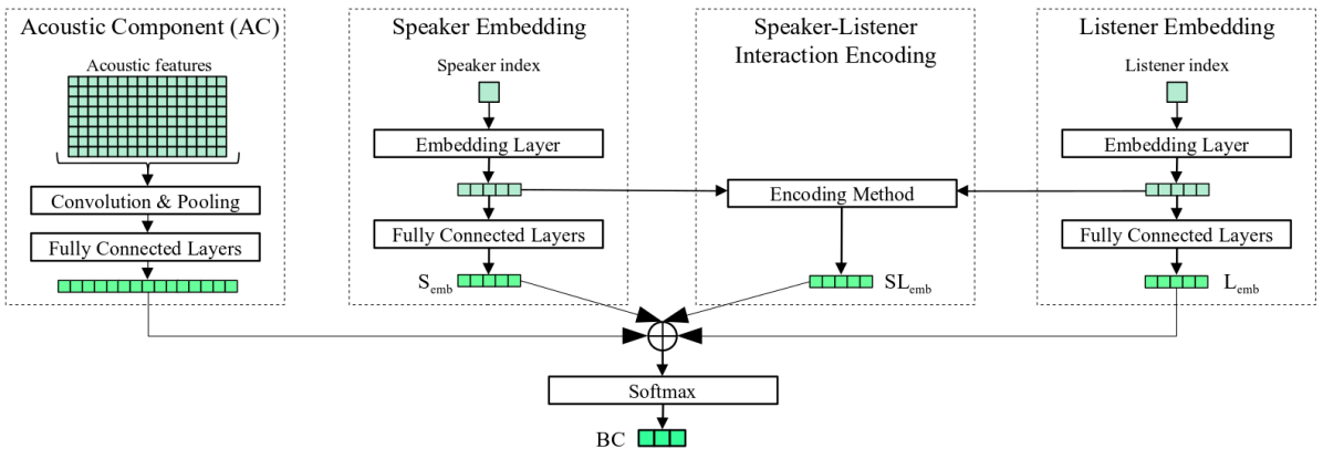
Figure 1: Backchannel prediction’s model with speaker-listener interaction. Our model is depicted with four constituents: acoustic component, speaker and listener embedding modules and the speaker-listener encoding mechanism. Not all constituents interact simultaneously, but different variants are introduced and described in Section 3 along with their outcome in Section 5. $\oplus$ represents a concatenation.

3 Proposed model

We introduce a BC predictor, depicted in Figure 1, that consists of an Acoustic Component (AC) and three behavior encoders, whose outputs are concatenated for posterior classification into No-BC, Yeah, or Uh-huh:

AC: An acoustic CNN that generates a vector representation from the frame-level MFCCs features of the last 2000 ms given a time point that are extracted from the speaker channel. This approach is based on ortega2019 . CNNs perform a discrete convolution using a set of different filters on an input matrix $w$, where each column corresponds to the frame-level MFCCs. We use 2D filters $f$ (with width $|f|$, i.e. number of consecutive frames) spanning over all dimensions $d$, i.e. number of MFCC features, as described by Equation 1.

$$\small(w\ast f)(x,y)=\sum_{i=1}^{d}\sum_{j=-|f|/2}^{|f|/2}w(i,j)\cdot f(x-i,y-j)$$ (1)

After convolution, the output is passed though a non-linear function, ReLU in this case, followed by a max-pooling operation in order to extract and concatenate the highest activation per filter, also known as feature map.

Listener embedding: It is an embedding layer, based on ortega2019 , followed by two FFNs. The embedding layer is a type of neural hidden layer that learns, encodes and stores dense vector representations of the listeners’ BC patterns in relation with the model input.

Speaker embedding: An embedding layer that encodes the speaker’s pattern. The mechanism is identical to the listener embedding.

SLI: encodes the speaker-listener interaction. We propose in Section 3.1 three speaker-listener interaction encoding mechanisms.

The AC is always present in the model, but not all behavior encoders interact simultaneously. Different variants are experimented and reported in Section 5.

Finally, the feature map and three resulting vectors from the behavior encoders, depending on the variant, are concatenated and passed to a softmax layer, that outputs a probability distribution over the three classes: No-BC, Yeah or Uh-huh.

3.1 Encoding speaker-listener interaction

Our hypothesis is that the interlocutors’ interaction can be modeled, i.e. encoding jointly the speaker and listener behaviors, and yield a positive impact on the overall model’s performance. Therefore, the three methods for encoding SLI presented below were implemented and tested during the experimentation phase. We follow this notation: $S_{emb}$ stands for speaker embedding, $L_{emb}$ for listener embedding and $SL_{emb}$ for speaker-listener interaction embedding. $S_{emb}$ and $L_{emb}$ are coming from two independent embedding layers.

Sum: This is the most simple approach and consists of summing up the interlocutor’s embeddings as in Equation 2.

$$\small SL_{emb}=S_{emb}+L_{emb}$$ (2)

Bilinear: A bilinear tranformation is applied to $S_{emb}$ and $L_{emb}$ and defined in Equation 3:

$$\small SL_{emb}=S_{emb}^{T}\;W\;L_{emb}+b$$ (3)

where $W\in\mathcal{R}^{d\times d\times k}$ stands for the learnable weight matrix, $n$ is the dimension of $S_{emb}$ and $L_{emb}$ and $k$ the dimension of $SL_{emb}$, and $b$ the bias term.

NTN: The goal of the NTN is to find and encode the relationship between two entity vectors across multiple dimensions socher2013reasoning ; ding2015deep , by computing a score ($SL_{emb}$) that defines how likely it is that the two entities are in a particular relationship. It is defined in Equation 4:

$$\small SL_{emb}=U^{T}\tanh\Bigl{(}S^{T}_{emb}\>W^{[1:k]}\>L_{emb}+V\begin{bmatrix}S_{emb}\\ L_{emb}\end{bmatrix}\Bigr{)}+b$$ (4)

where $tanh$ is applied element-wise, $W^{[1:k]}\in\mathcal{R}^{n\times n\times k}$ is a learnable weight matrix and $S^{T}_{emb}\>W^{[1:k]}\>L_{emb}$ stands for a bilinear transformation, already introduced in Equation 3, but applied $k$ times, each entry takes a slice of $W$. $V\in\mathcal{R}^{k\times 2d}$, $U\in\mathcal{R}^{k}$ and $b$ (bias) are learnable parameters socher2013reasoning .

4 Experimental setup

We experimented on two corpora: SwDA for English and GECO for German. We present their specs and statistics on Section 4. Our data annotations, described below, are available in the project repository.

Table 1: Statistics for SwDA and GECO datasets and their class distribution.

	SwDA		GECO
	Counts	%	Counts	%
Yeah	15,380	19.3	2,026	24.3
Uh-huh	24,436	30.7	2,149	25.7
No-BC	39,816	50.0	4,175	50.0
Conversations	2438	–	46	–
Interlocutors	520	–	13	–

4.1 The Switchboard Dialog Act Corpus

SwDA jurafsky1997switchboard is a dialog corpus of telephone English conversations annotated at dialog-act level, including BCs . Annotations and time stamps for general BCs are from jurafsky1997switchboard , while for No-BC instances, splits and time stamps are taken from ruede2017 . According to the authors, the latter time stamps were chosen from a few seconds of speech before each BC from the speaker speech to constitute negative samples (BC absence) and they motivate it by assuming that during those periods the listener decided not to backchannel regardless of what the speaker was saying. With respect to the splits, from a total of 2,438 conversations, 2,000 are for training, 200 for validation and 238 for testing. We used the categorization proposed and mentioned in Section 1, i.e recipiency tokens used for backchanneling Yeah vs Uh-huh. For that purpose, we manually annotated the BC tokens and kept those that fitted into both categories.

Our annotation process for BC was as follows, we extracted a list of 670 unique utterances used within the corpus to backchannel. In the category Uh-huh, we included all BC realizations like uh-huh, um-hum and other variants, that describe passive recipiency. For the second category Yeah, we included all BC realizations like yeah, yes, yep and other variants, that express alignment to the speaker. We excluded variants with the marker [laughter], because the laughter assesses the speaker’s talk and does not meet the canonical use of these minimal responses that we investigate. Any other BC realization, marker or combination was discarded.

During the annotation process, 84 unique BC realizations out of 670 were finally included, 57 for the category Yeah and 27 for Uh-huh. As result, our data consists of 15.4k Yeah instances and 22.4k of Uh-huh, summing up to 39.8k BC instances and the same amount for No-BC.

For speaker/listener annotation, SwDA provides the mapping between dialog channels and unique interlocutors. On average, each speaker takes part in 10 conversations. Official documentation reports 543 unique participants, but the annotation does not include the speaker ID in 11 channels. Therefore, we followed ortega2020oh ’s suggestion and a random speaker was assigned to those channels, ending up with 520 unique interlocutor IDs.

4.2 GErman COrpus database

GECO schweitzer2013conv consists of 46 two-party dialogs in German between unacquainted female subjects. 22 conversations took place in a unimodal setting, where participants could not see each other, while for the remaining 24 dialogs subjects were facing each other.

BC annotation was done heuristically based on acoustic and lexical information, because no manual annotation was available. An utterance expressed during another person’s turn is regarded as BC if its duration is less than one second, or if all its words are covered in a manually generated list of German BC expressions. The list contains common single-word BC like ja (yes) and hm, multi-word expressions like oh mein Gott (oh my god), and intensifiers for BC such as voll (very) in voll cool (really cool).

During the initial annotation process, 1,657 utterances were marked as unique BC realizations. However, after manual checking, 1,005 were considered BCs and the rest false positives. For Yeah vs Uh-huh, we followed the same annotation procedure explained in Section 4.1 . For the former, we included the terms ja and other variants, while for the latter hm hm, mh mh and mhm mhm. Finally, 91 unique BC realizations were included in the dataset, 37 for the category Yeah and 54 for Uh-huh. As result, our data consists of 2k Yeah instances and 2.1k of Uh-huh, summing up to 4.1k BC instances and the same amount for No-BC. We followed the method from ruede2017 , described in Section 4.1, to select No-BC instances.

4.3 Acoustic features extraction

As mentioned in Section 4.1 and Section 4.2, we obtained the time stamps for all instances in the dataset that were later used to extract acoustic features of the 2000 ms from the speaker speech signal before the BC happens.

ortega2020oh experimented with MFCCs and prosodic features on BC modeling and found that MFCCs features yield better results. Therefore, we also consider 13 MFCCs features that were extracted using the openSMILE toolkit tools:openSMILE at frame level, i.e. the speech signal is divided into frames of 25 ms with a shift of 10 ms.

5 Experimental results

We present the results of model variants trained on both datasets. All variants include the AC depicted in Figure 1, and they differ by the components that are concatenated, i.e. speaker embedding (S), listening embedding (L) and SLI embedding. The hyperparameter ranges used for experimentation are presented in Section 5. The listener and speaker embeddings are 5-dim vectors.

Table 2: Range values used for the hyperparameter search during the model training and fixed values for the most relevant hyperparameters of the model architecture.

Hyperparameter	Value
Filter widths	[10, 11, 12]
Number of filters	[16, 32, 64, 128]
Dropout rate	[0.1, 0.3, 0.5]
Pooling size	(10, 1)
Acoustic features	MFCC
Number of speech frames	[48, 98, 148, 198]
Mini-batch size	[16, 32, 64, 128]
Embedding length	5

Our first experiments aimed to explore the performance of the AC, our baseline, and the effect of concatenating the embeddings. Results are shown in the upper part of Section 5. They were obtained on the test set when the best performance was found on the validation set. On SwDA, the AC reached an 56.9% in accuracy and 0.42 in F1-score. By concatenating the speaker embedding (AC $\oplus$ S), both the accuracy and F1-score show a slight improvement. Whereas by concatenating the listener embedding (AC $\oplus$ L), the metrics improve even further, reaching 60.3% and 0.52 in accuracy and F1-score, accordingly. Finally, we concatenated both embeddings (AC $\oplus$ S $\oplus$ L) and a slight extra boost was reached in both metrics, bringing an improvement of 3.8% in accuracy and 0.11 in F1-score in comparison with the baseline.

On GECO, the trend of the results is slightly different. The AC reached an 49.3% in accuracy terms and 0.35 in F1-score. The accuracy is not even reaching 50%, i.e. the majority class No-BC in our setup. Nonetheless, by concatenating the speaker embedding, both metrics improved, the accuracy reaching 55.1% and the F1-score 0.42. We take this scenario as our baseline on this dataset. Unlike the experiments on SwDA, when AC and the listener embeddings interact, the performance drops drastically. Finally, we concatenated both embeddings and as outcome both metrics improved in comparison with the baseline, reaching 60.0% in accuracy and 0.44 in F1-score.

Table 3: Accuracy (%) and F1-score for AC (row 1), its variants with concatenated embeddings (rows 2-4) and with methods encoding the speaker-listener interaction (lower part, rows 5-7). $\oplus$ stands for concatenation.

Model	SwDA		GECO
	Accuracy	F1-score	Accuracy	F1-score
Acoustic (AC)	56.9	0.42	49.3	0.35
AC $\oplus$ Speaker (S)	59.7	0.46	55.1	0.42
AC $\oplus$ Listener (L)	60.3	0.52	44.9	0.38
AC $\oplus$ S $\oplus$ L	60.7	0.53	60.0	0.44
AC $\oplus$ SLI-Sum	60.5	0.54	62.7	0.49
AC $\oplus$ SLI-Bilinear	58.8	0.50	58.2	0.37
AC $\oplus$ SLI-NTN	61.0	0.55	64.7	0.51

5.1 Effect of encoding mechanisms

We found that the embeddings let the model make more accurate predictions. Therefore, we experimented with the three mechanisms to encode the SLI from Section 3.1: Sum, Bilinear and NTN. Our intuition behind this was that a more sophisticated mechanism could capture better the interaction between the interlocutors, and ultimately it would improve the BC prediction. The lower part of Section 5 contains these results.

We took the model variant AC$\oplus$S$\oplus$L as baseline to be compared with the SLI encoding mechanisms. On SwDA, the embedding Sum does not provide any improvement. Moreover, the Bilinear approach even affects the performance. Finally, the NTN showed a slight boost on both metrics, 61.0% for accuracy and 0.55 for F1-score. On GECO, the embedding Sum enhances the model performance to 62.7% on accuracy and 0.49 on F1-score, whereas the Bilinear mechanism exerts negative influence on both metrics with respect to the current baseline. At last, the NTN surpassed the rest of the previous mechanisms ending up at 64.7% on accuracy and 0.51 in F1-score.

On both datasets, the Bilinear approach affected negatively the performance, showing that it is not suitable for encoding the SLI. The Sum mechanism helped on GECO, but not on SwDA, leading to no conclusive interpretation. Conversely, the NTN mechanism substantially enhanced the model performance.

Although considerable improvements on accuracy can be consistently seen during the experiments, the best performing model on both datasets is still far from solving the task. We thus inquire deeper into the model results in Section 5.2.

5.2 Effect of class distribution

The class distribution is skewed and the accuracy analysis is not enough. Therefore, we look closer at macro F1-scores and per class. On the one hand, the improvement is notable when we compare macro F1-scores from AC (baseline) vs AC$\oplus$SLI-NTN (best performing model) on both datasets, see Section 5. On the other hand, when we look at the F1-score per class from the model AC$\oplus$SLI-NTN on both datasets, the dominance of the No-BC class becomes evident, see Section 5.2.

Table 4: F1-scores per class on both datasets from the model variant: AC$\oplus$SLI-NTN.

	Dataset	F1-score
		No-BC	Yeah	Uh-huh
	SwDA	0.70	0.35	0.58
	GECO	0.78	0.18	0.56

The model performs fairly well on classes No-BC and Uh-huh, but struggles with the category Yeah. We hypothesize two possible reasons: (1) the class Yeah is the smallest in the dataset, and (2) the elicitation of acknowledging responses, like Yeah, depends more on lexical and semantic information gardner1998between that are not currently considered in this investigation scope. The integration of such information and the mechanism to process it are left as future work.

6 Exploring the listeners embeddings

We observed the contributions of encoding the SLI. Therefore, we decided to experiment and analyze even further the trained interlocutors’ embeddings, especially the listeners embeddings from two model variants: AC$\oplus$L (best performing model without interaction encoding) and AC$\oplus$SLI-NTN (best performing model with interaction encoding). The former model only learns listener embeddings, while the latter model learns jointly listener and speaker embeddings.

6.1 Impact of listener embeddings

Given that each listener embedding encodes the BC behavior, we wanted to know at which extent a particular embedding can help the model to accurately predict BCs, even in conversations where this embedding did not originally take part. To accomplish this goal, the model made predictions for the whole test set using only one of listener embeddings at a time and we calculated the corresponding F1-score. This series of predictions results in four F1-score distributions, one per model variant vs. dataset, depicted in Figure 2.

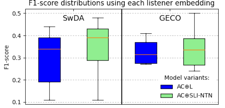
Figure 2: F1-score distributions for predicting BC using each listener embedding separately on SwDA (left side) and GECO (right side). Distributions in blue (darker) correspond to AC$\oplus$L, whereas distribution in green (lighter) to AC$\oplus$SLI-NTN.

From the F1-score distributions on SwDA, we found that the model AC$\oplus$L achieved the highest F1-score of 0.44 (mean=0.29, median=0.34), whereas the model AC$\oplus$SLI-NTN achieved the highest F1-score of 0.48 (mean=0.35, median=0.39). Furthermore, by directly comparing listeners on both scenarios, 437 listeners out of 520 (84.0%) led to an improvement in terms of F1-score, 0.06 on average, but within the interval [-0.14, 0.28].

Similar findings come from the F1-score distribution on GECO, although the number of unique interlocutors is comparably smaller. While the highest F1-score from the model AC$\oplus$L was 0.40 (mean=0.33, median=0.32), the model AC$\oplus$SLI-NTN scored 0.50 (mean=0.34, median=0.32) as maximum. Finally, seven listeners out of 13 showed an improvement of 0.02 in F1-score on average, within the interval [-0.14, 0.16].

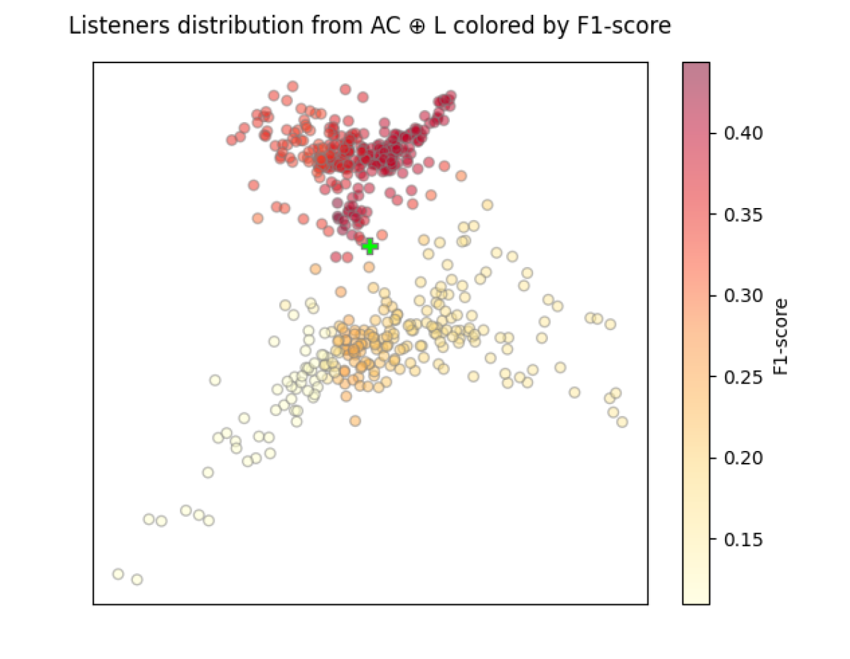
Figure 3: PCA-reduced listeners embeddings distribution from the model variant AC$\oplus$L on SwDA. Axes correspond to the the principal components. Centroid appears as a green cross. The color of each dot represents the F1-score according to the bar on the right.

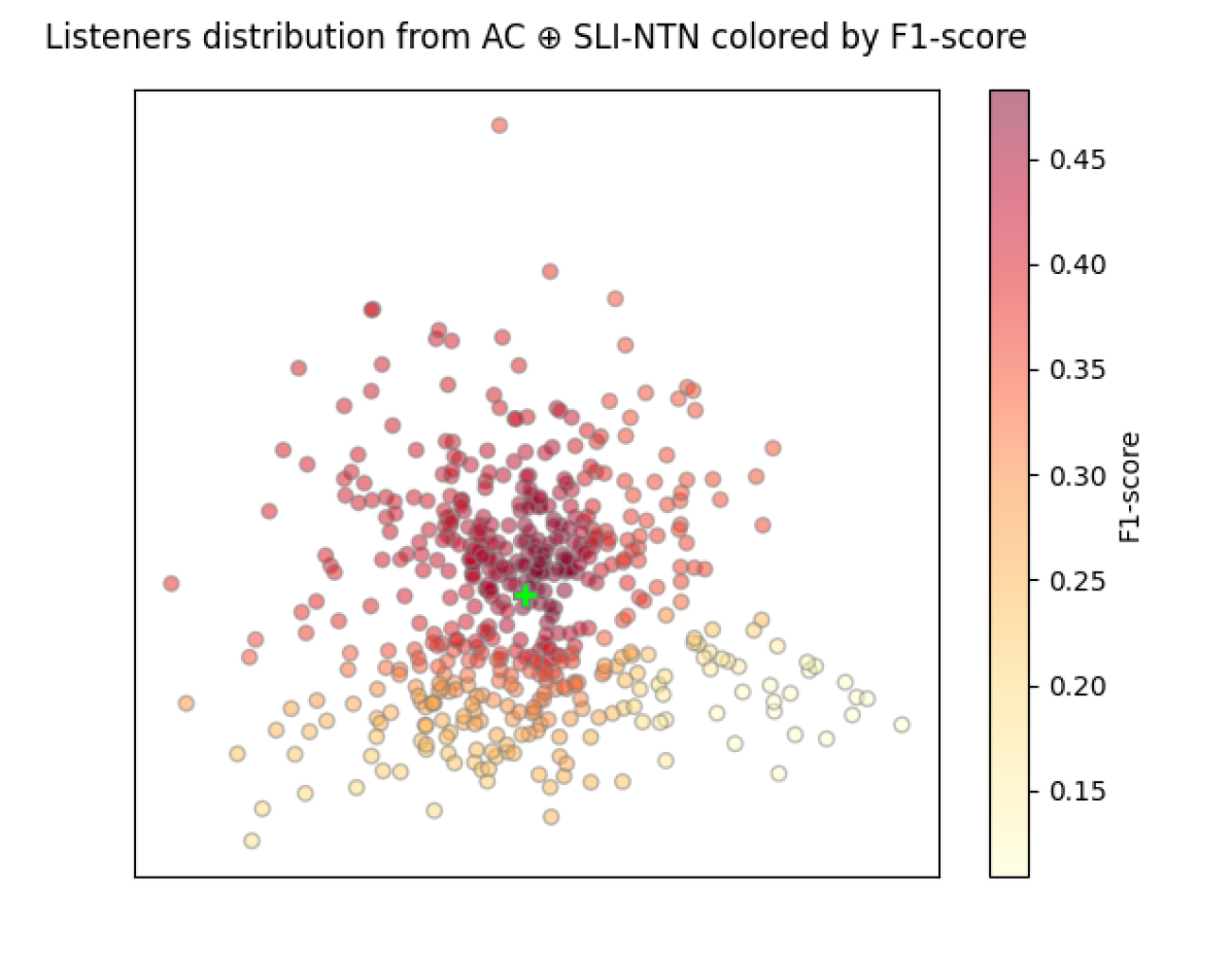
Figure 4: PCA-reduced listeners embeddings distribution from the model variant AC$\oplus$SLI-NTN on SwDA. Axes correspond to the the principal components. Centroid appears as a green cross. The color of each dot represents the F1-score according to the bar on the right.

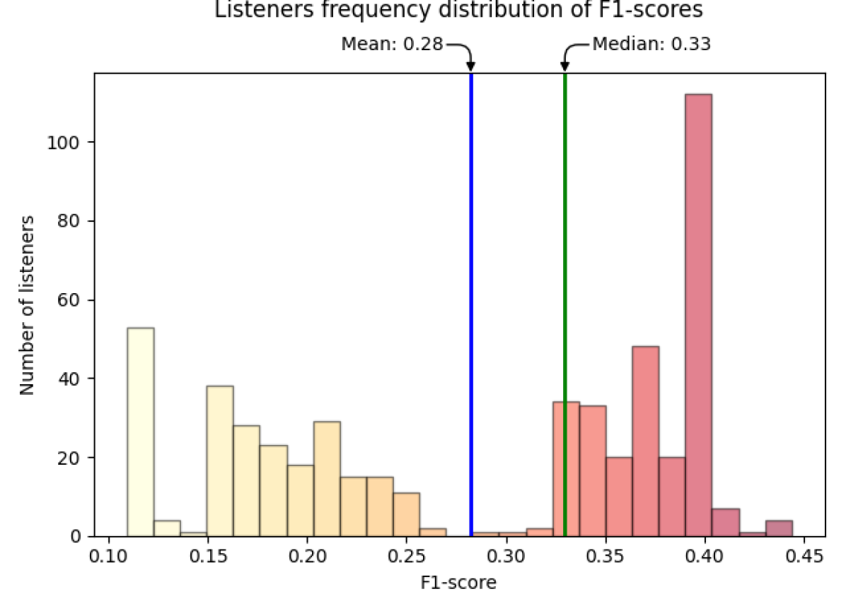
Figure 5: Listeners frequency distribution obtained from the model variant AC$\oplus$L on SwDA. Mean and median are depicted numerically and with vertical lines, blue and green, respectively.

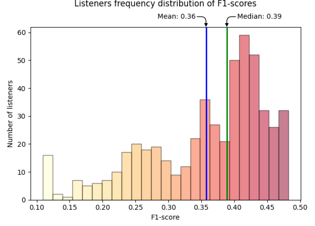
Figure 6: Listeners frequency distribution obtained from the model variant AC$\oplus$SLI-NTN on SwDA. Mean and median are depicted numerically and with vertical lines, blue and green, respectively.

6.2 A closer look at the embedding space

We inspected the listeners embeddings and the F1-score distributions from both models variants analyzed in previous Section 6.1. Nevertheless, we restricted our investigation to SwDA, because of the vast number of unique listeners.

Initially, we extracted the listeners embeddings from each model variant and applied principal component analysis (PCA) to reduce the embedding dimensionality from five to two dimensions, in order to be 2D-plotted as listener distributions. They can be seen on Figure 6 and Figure 6. The former corresponds to the model AC$\oplus$L, while the latter to AC$\oplus$SLI-NTN. Each dot represents one speaker embedding and its color intensity the F1-score, according to the color scale on the right. The green cross represents the centroid of the distribution.

Figure 6 and Figure 6 depict the frequency distribution of F1-score in 25 intervals, corresponding to the model variant AC$\oplus$L and AC$\oplus$SLI-NTN, respectively, including the mean (blue line) and the median (green line).

With respect to the listeners’ embedding distribution from AC$\oplus$L, Figure 6, we can observe two clear clusters, one above (redder/darker) and one below (more yellow/lighter) the centroid. The upper cluster concentrates the majority of listeners embeddings that help the model variant AC$\oplus$L achieve the highest F1-scores. It is important to remark that embeddings do not tend to concentrate around the centroid. The frequency distribution on Figure 6 also shows the two aforementioned clusters, with few embeddings in the middle.

Regarding with the listeners’ embedding distribution from AC$\oplus$SLI-NTN, Figure 6, it behaves differently. The embeddings cluster more uniformly and the reddest/darkest areas concentrate around the centroid. Nonetheless, the upper area groups the the majority of listeners embeddings that help the model variant AC$\oplus$SLI-NTN achieve the highest F1-scores. The frequency distribution from Figure 6 shows that most of the listener embeddings accumulate on the right side, the area containing the higher F1-scores.

As future work, we consider a more extensive analysis that includes the relation between characteristics linked to a specific listener, e.g. the F1-score vs the number of BCs in the training set and the number of conversations with unique speakers.

7 Conclusions

In this paper, we presented a novel approach for backchannel prediction characterized by three aspects: 1) it is motivated by minimal recipiency theory, i.e. the canonical use of minimal responses Yeah and Uh-huh in both English and German, 2) it encodes the speaker and listener behavior, and 3) it models the speaker-listener interaction performing three different mechanisms. Additionally, we implemented a semi-automatic and heuristic annotation on the corpora SwDA and GECO that is publicly available for further research.

Our experimental results on both datasets showed that by combining the acoustic component with either the listener or the speaker embeddings, the model performance steadily improves. More importantly, the speaker-listener interaction helped the model reach its best overall performance. Finally, by exploring and experimenting with the listeners embeddings from two model variants on SwDA, we found that 84.0% of the listener embeddings helped the model to make more asserted predictions, when they were learnt jointly with the speaker embeddings.

AdaGrad

adaptive gradient algorithm

AM

attention mechanism

CRF

conditional random field

CNN

convolutional neural network

LSTM

long short-term network

FFN

feed-forward network

DA

dialog act

DL

deep learning

E2E

End-to-End

SGD

stochastic gradient descent

HMM

hidden Markov model

NLP

natural language processing

RNN

recurrent neural network

SVM

support vector machine

SWBD

Switchboard Corpus

SwDA

The Switchboard Dialog Act Corpus

ASR

automatic speech recognition

NN

neural network

MTs

manual transcriptions

ATs

automatic transcriptions

E2E

End-to-End

CD

context-dependent

TDNN

time-delay neural network

CTC

connectionist temporal classification

WER

word error rate

MFCC

Mel-frequency cepstral coefficient

GMM

Gaussian Mixture Model

ESPnet

End-to-End Speech Processing Toolkit

BC

backchannel

GECO

GErman COrpus

NTN

Neural Tensor Network

AC

Acoustic Component

PCA

principal component analysis

SLI

speaker-listener interaction

ML

machine learning

References

- (1) Al Moubayed, S., Baklouti, M., Chetouani, M., Dutoit, T., Mahdhaoui, A., Martin, J.C., Ondas, S., Pelachaud, C., Urbain, J., Yilmaz, M.: Generating robot/agent backchannels during a storytelling experiment. In: 2009 IEEE International Conference on Robotics and Automation, pp. 3749–3754. IEEE (2009)
- (2) Bavelas, J.B., Gerwing, J.: The listener as addressee in face-to-face dialogue. International Journal of Listening 25(3), 178–198 (2011)
- (3) Blache, P., Abderrahmane, M., Rauzy, S., Bertrand, R.: An integrated model for predicting backchannel feedbacks. In: Proceedings of the 20th ACM International Conference on Intelligent Virtual Agents, pp. 1–3 (2020)
- (4) Brunner, L.J.: Smiles can be back channels. Journal of personality and social psychology 37(5), 728 (1979)
- (5) Clancy, P.M., Thompson, S.A., Suzuki, R., Tao, H.: The conversational use of reactive tokens in English, Japanese, and mandarin. Journal of Pragmatics 26, 355–387 (1996)
- (6) Clark, H.H., Krych, M.A.: Speaking while monitoring addressees for understanding. Journal of memory and language 50(1), 62–81 (2004)
- (7) Devlin, J., Chang, M.W., Lee, K., Toutanova, K.: Bert: Pre-training of deep bidirectional transformers for language understanding. arXiv preprint arXiv:1810.04805 (2018)
- (8) Ding, X., Zhang, Y., Liu, T., Duan, J.: Deep learning for event-driven stock prediction. In: Twenty-fourth international joint conference on artificial intelligence (2015)
- (9) Ekstedt, E., Skantze, G.: Voice activity projection: Self-supervised learning of turn-taking events. In: INTERSPEECH 2022, pp. 5190–5194. International Speech Communication Association (2022)
- (10) Eyben, F., Weninger, F., Gross, F., Schuller, B.: Recent developments in opensmile, the munich open-source multimedia feature extractor. In: Proc. of ACM Multimedia (2013)
- (11) Gardner, R.: Between speaking and listening: The vocalisation of understandings1. Applied linguistics 19(2), 204–224 (1998)
- (12) Goodwin, C.: Between and within: Alternative sequential treatments of continuers and assessments. Human studies 9(2), 205–217 (1986)
- (13) Gravano, A., Hirschberg, J.: Backchannel-inviting cues in task-oriented dialogue. In: Proc. of Interspeech (2009)
- (14) Hara, K., Inoue, K., Takanashi, K., Kawahara, T.: Prediction of turn-taking using multitask learning with prediction of backchannels and fillers. Listener 162, 364 (2018)
- (15) Heinz, B.: Backchannel responses as strategic responses in bilingual speakers’ conversations. Journal of pragmatics 35(7), 1113–1142 (2003)
- (16) Ishii, R., Ren, X., Muszynski, M., Morency, L.P.: Multimodal and multitask approach to listener’s backchannel prediction: Can prediction of turn-changing and turn-management willingness improve backchannel modeling? In: Proceedings of the 21st ACM International Conference on Intelligent Virtual Agents, pp. 131–138 (2021)
- (17) Jain, V., Leekha, M., Shah, R.R., Shukla, J.: Exploring semi-supervised learning for predicting listener backchannels. In: Proceedings of the 2021 CHI Conference on Human Factors in Computing Systems, pp. 1–12 (2021)
- (18) Jefferson, G.: Notes on a systematic deployment of the acknowledgement tokens “yeah” and “mm hm”. Papers in Linguistics 17, 197–206 (1984)
- (19) Jurafsky, D., Shriberg, E.: Switchboard swbd-damsl shallow-discourse-function annotation coders manual. Institute of Cognitive Science Technical Report (1997)
- (20) Kawahara, T., Yamaguchi, T., Inoue, K., Takanashi, K., Ward, N.G.: Prediction and generation of backchannel form for attentive listening systems. In: Interspeech, pp. 2890–2894 (2016)
- (21) Maynard, S.K.: Analyzing interactional management in native/non-native English conversation: A case of listener response. IRAL, International Review of Applied Linguistics in Language Teaching 35(1), 37 (1997)
- (22) McGregor, G., White, R.S.: Introduction. In: G. McGregor, R.S. White (eds.) Reception and response: Hearer creativity and the analysis of spoken and written texts, pp. 1–7. Routledge (2015)
- (23) Morency, L.P., de Kok, I., Gratch, J.: A probabilistic multimodal approach for predicting listener backchannels. Journal of Autonomous Agents and Multi-Agent Systems pp. 70–84 (2010)
- (24) Ortega, D., Li, C.Y., Vallejo, G., Denisov, P., Vu, N.T.: Context-aware neural-based dialog act classification on automatically generated transcriptions. In: Proc. of ICASSP (2019)
- (25) Ortega, D., Li, C.Y., Vu, N.T.: Oh, jeez! or uh-huh? a listener-aware backchannel predictor on asr transcriptions. In: ICASSP 2020-2020 IEEE International Conference on Acoustics, Speech and Signal Processing (ICASSP), pp. 8064–8068. IEEE (2020)
- (26) Park, H.W., Gelsomini, M., Lee, J.J., Breazeal, C.: Telling stories to robots: The effect of backchanneling on a child’s storytelling. In: 2017 12th ACM/IEEE International Conference on Human-Robot Interaction (HRI, pp. 100–108. IEEE (2017)
- (27) Poppe, R., Truong, K.P., Heylen, D.: Backchannels: Quantity, type and timing matters. In: International Workshop on Intelligent Virtual Agents, pp. 228–239. Springer (2011)
- (28) Ruede, R., Müller, M., Stüker, S., Waibel, A.: Enhancing backchannel prediction using word embeddings. In: Proc. of Interspeech (2017)
- (29) Schegloff, E.A.: Discourse as an interactional achievement: Some uses of ‘uh huh’and other things that come between sentences. Analyzing discourse: Text and talk 71, 93 (1982)
- (30) Schweitzer, A., Lewandowski, N.: Convergence of articulation rate in spontaneous speech. In: Proc. of Interspeech (2013)
- (31) Socher, R., Chen, D., Manning, C.D., Ng, A.: Reasoning with neural tensor networks for knowledge base completion. In: Advances in neural information processing systems, pp. 926–934 (2013)
- (32) Solorio, T., Fuentes, O., Ward, N.G., Al Bayyari, Y.: Prosodic feature generation for back-channel prediction. In: Proc. of Interspeech (2006)
- (33) Tolins, J., Tree, J.E.F.: Addressee backchannels steer narrative development. Journal of Pragmatics 70, 152–164 (2014)
- (34) Truong, K.P., Poppe, R., Heylen, D.: A rule-based backchannel prediction model using pitch and pause information. In: Eleventh Annual Conference of the International Speech Communication Association. Citeseer (2010)
- (35) Ward, N.: Using prosodic clues to decide when to produce back-channel utterances. In: Proc. of ICSLP, pp. 1728–1731 (1996)
- (36) Ward, N., Tsukahara, W.: Prosodic features which cue back-channel responses in English and Japanese. Journal of Pragmatics pp. 1177–1207 (2000)
- (37) Ward, N.G.: Backchannel facts (2017). URL https://www.cs.utep.edu/nigel/bc. Accessed: 2020-03-23
- (38) Ward, N.G., Escalante, R., Al Bayyari, Y., Solorio, T.: Learning to show you’re listening. Computer Assisted Language Learning 20(4), 385–407 (2007)
- (39) Xudong, D.: Listener response. The pragmatics of interaction 4, 104 (2009)
- (40) Yngve, V.: On getting a word in edgewise. In: Proc. of CLS 16 (1970)