Missing Data Imputation with Graph Laplacian Pyramid Network

Abstract

Data imputation is a prevalent and important task due to the ubiquitousness of missing data. Many efforts try to first draft a completed data and second refine to derive the imputation results, or “draft-then-refine” for short. In this work, we analyze this widespread practice from the perspective of Dirichlet energy. We find that a rudimentary “draft” imputation will decrease the Dirichlet energy, thus an energy-maintenance “refine” step is in need to recover the overall energy. Since existing “refine” methods such as Graph Convolutional Network (GCN) tend to cause further energy decline, in this work, we propose a novel framework called Graph Laplacian Pyramid Network (GLPN) to preserve Dirichlet energy and improve imputation performance. GLPN consists of a U-shaped autoencoder and residual networks to capture global and local detailed information respectively. By extensive experiments on several real-world datasets, GLPN shows superior performance over state-of-the-art methods under three different missing mechanisms. Our source code is available at https://github.com/liguanlue/GLPN.

1 Introduction

Missing data is ubiquitous and has been regarded as a common problem encountered by machine learning practitioners in real-world applications [1, 2, 3, 4]. In industries, for example, faulty sensors may cause errors or missingness during data collection, which bring challenges to state prediction and anomaly detection [5]. In previous works, a popular paradigm for missing data imputation is the “draft-then-refine” procedure [3, 6, 7, 1, 8, 9, 10, 11, 12]. As the name suggests, it first uses basic methods (e.g., mean) to perform a draft imputation of the missing attributes. Then, the completed feature matrix is fed to more sophisticated methods (e.g., graph neural networks [9]) for refinement. However, there is a lack of principle to guide the design of such “draft-then-refine” procedures: Under what conditions are these two steps complementary? Which aspects of the imputation are important?

In this work, we initialize the first study to examine such a “draft-then-refine” paradigm from the perspective of Dirichlet energy [13], in which it measures the “smoothness” among different observations. Surprisingly, we find that some rudimentary “draft” steps of the paradigm, e.g., mean and KNN, will lead to a notable diminishment of Dirichlet energy. In this vein, an energy-maintenance “refine” step is in urgent need to make the two steps complementary and recover the overall energy. However, we find that many popular methods in “refine” step also lead to a diminishment of Dirichlet energy. For example, Graph Convolution Networks (GCNs) [14, 15] have been widely used to serve as a “refine” step [11, 10]. Nevertheless, GCN based models suffer from over-smoothness and lead to rapid Dirichlet energy decline [16, 17, 13]. Considering the above property of GCNs, applying GCN-based models during the “refine” step will cause further Dirichlet energy diminishment. It means the final imputation may be relatively over-smooth, which is far from accurate imputation from the perspective of energy maintenance.

Another challenge of the missing data imputation is the shift in global and local distribution in data matrices. Global methods [18, 19, 20] prioritize generating data that approximates the distribution of the original data as a whole, but they may fail to capture the detailed representation of local patterns such as the boundary between clusters. In contrast, local methods [21, 22, 23, 24] rely on the local similarity pattern to estimate missing values by aggregating information from neighboring data points. However, they may underperform because they disregard global information.

Regarding the concerns above, we propose a novel deep imputation framework, Graph Laplacian Pyramid Network (GLPN). We utilize the graph structure to handle the underlying relational information, where the incomplete data matrix represents node features [25]. The proposed GLPN, consisting of a U-shaped autoencoder and learnable residual networks, has been proven to maintain the Dirichlet energy under the “draft-then-refine” paradigm. Specifically, the pyramid autoencoder [26] learns hierarchical representations and restores the global (low-frequency) information. Based on graph deconvolutional networks [9], the residual network focuses on recovering local (high-frequency) information on the graph. The experiment results on heterophilous and homophilous graphs show that GLPN consistently captures both low- and high-frequency information leading to better imputation performance compared with the existing methods.

To sum up, the contributions of our work are as follows:

• We analyze general missing data imputation methods with a “draft-then-refine” paradigm from the perspective of Dirichlet energy, which could be connected with the quality of imputation.

• Considering the Dirichlet energy diminishment of GCN based methods, we propose a novel Graph Laplacian Pyramid Network (GLPN) to preserve energy and improve imputation at the same time.

• We conduct experiments on three different categories of datasets, including continuous sensor datasets, single-graph datasets comprising heterophilous and homophilous graphs, and multi-graph datasets. We evaluated our proposed model on three different types of missing data mechanisms, namely MCAR, MAR, and MNAR.

• The results demonstrate that the GLPN outperforms the state-of-the-art imputation methods, exhibiting remarkable robustness against varying missing ratios. Additionally, our model displays a superior ability to maintain Dirichlet energy, further substantiating its effectiveness in imputing missing data.

The remainder of this paper is organized as follows. Section 2 introduces the related work of imputation methods, the laplacian pyramid and Graph U-Net. Section 3 illustrates the task definition and Graph Dirichlet Energy. Meanwhile, a proposition has been introduced to analyze the energy changing of the “draft-then-refine” imputation paradigm. Section 4 presents the details of the proposed model and Section 5 provides the analysis of energy maintenance. In Section 6, we evaluate our method on several real-world datasets to show the superiority of our proposed model. Finally, we draw our conclusion in Section 7.

2 Related Work

2.1 Data Imputation

Classical imputation methods [27] can be divided into generative and discriminative models. Generative models include the Expectation Maximization (EM) [28, 29], Autoencoder [30], variational autoenncoders [31, 32], and Generative Adversarial Nets (GANs) [33]. Discriminative methods include matrix completion [34, 35, 18, 36], multivariate imputation by chained equations [6], optimal transport based distribution matching [27], iterative random forests [37], and causally-aware imputation [3]. However, both two types overlook the relationship between different observations, i.e., additional graph information.

Recently, several works have extended the Graph Neural Networks (GNNs) to make use of this relational information. GRAPE considers observations and features as two types of nodes in bipartite networks [38]. GDN proposes to use graph deconvolutional networks to recover input signals as imputation [9]. GCNMF adapts GCNs to predict the missing data based on a Gaussian mixture model [10]. IGNNK utilizes Diffusion GCN to do graph interpolation and estimate the feature of unseen nodes [11]. However, existing GNNs based models tend to give smooth representations for all the observations and lead to an inevitable decrease in graph Dirichlet energy, which will degrade the imputation performance.

Meanwhile, based on the methods used, missing data imputation can also be categorized into two types: global and local approaches. The global approach [39, 40] predicts missing values considering the global correlation information derived from the entire data matrices. However, this assumption may not adequate where each sample exhibits a dominant local similarity structure. In contrast, the local approach [41] exploits only the local similarity structure to estimate the missing values by computing them from the subset with high correlation. The local imputation technique may perform less accurately than the global approach in homophilous data. To address this limitation, we proposed a hybrid hierarchical method that combines both global and local patterns and is suitable for both homophilous and heterophilous data which could be verified by extensive experiments.

2.2 Laplacian Pyramid and Graph U-Net

The laplacian pyramid is first proposed to do hierarchical image compression [42]. Combining with deep learning framework, deep laplacian pyramid network targets the task of image super-resolution, which reconstructs a high-resolution image from a low-resolution input [43, 44, 45]. The main idea of the deep laplacian pyramid network is to learn high-frequency residuals for reconstructing image details, which motivates the residual network design in our proposed model. Graph U-Net [46], consisting of the graph pooling-unpooling operation and a U-shaped encoder-decoder architecture, has been proposed for node classification on graphs. However, Graph U-Net uses skip connection instead of learnable layers as residuals, which would cause over-smoothing node representations and decrease the graph Dirichlet energy, if it is adopted directly for missing data imputation. Besides, some work introduce hierarchical “Laplacian pyramids” for data imputation [47, 48]. The Laplacian pyramids in these methods are composed of a series of functions in a multi-scale manner. Differently, the Laplacian pyramid indicates a series of graphs with different scales in our work.

3 Preliminaries

3.1 Task Definition

Let $\bm{X}\in\mathbb{R}^{n\times d}$ be a data matrix consisting of $n$ observations with $d$ features for each observation. $\bm{X}_{i,j}$ denotes the $j^{th}$ feature of $i^{th}$ observation. To describe the missingness in the data matrix, we denote $\bm{M}\in\{0,1\}^{n\times d}$ as the mask matrix, where $\bm{X}_{i,j}$ can be observed only if $\bm{M}_{i,j}=1$. We assume that there exists some side information describing the relationship between different observations, e.g., graph structure. We consider each observation as a node on graph and model the relationship by the adjacency matrix $\bm{A}\in\mathbb{R}^{n\times n}$.

Task Definition. Given the observed feature matrix $\bm{X}^{\star}$, mask matrix $\bm{M}$, graph structure $\bm{A}$, the imputation algorithm aims to recover the missingness of data matrix by

$$\bm{\hat{X}}=f\left(\bm{X}^{\star},\bm{A}\right),$$

where $\bm{X}^{\star}_{i,j}=\begin{cases}\mathrm{NA},&\text{if }\bm{M}_{i,j}=0\\ \bm{X}_{i,j},&\text{ otherwise }\end{cases}$, $\mathrm{NA}$ represents a missing value, and $f:(\mathbb{R}\cup\{\mathrm{NA}\})^{n\times d}\rightarrow\mathbb{R}^{n\times d}$ denotes a learnable imputation function.

3.2 Graph Dirichlet Energy

Intuitively, the graph Dirichlet energy measures the “smoothness” between different nodes on the graph [13]. It has been used to measure the expressiveness of the graph embeddings. For data imputation, in the case of reduced graph Dirichlet energy, the recovered missing data suffers from “over-smoothed” imputation, which leads to poor imputation performance.

Definition 3.1 (Graph Dirichlet Energy).

Given the node feature matrix $X\in\mathbb{R}^{n\times d}$, the corresponding Dirichlet Energy is defined by:

where $tr(\cdot)$ denotes the trace of a matrix and $\parallel\cdot\parallel$ is the $\ell^{2}$-norm. $\bm{X}_{i,:}$ is the $i^{th}$ row of feature matrix $\bm{X}$ corresponding to the features of the $i^{th}$ node. $\bm{D}_{i,i}$ is the $i^{th}$ element on the diagonal of the degree matrix $\bm{D}$. $\tilde{\Delta}:=\bm{I}_{n}-\tilde{\bm{D}}^{-\frac{1}{2}}\tilde{\bm{A}}\tilde{\bm{D}}^{-\frac{1}{2}}$ is the augmented normalized Laplacian matrix, where $\tilde{\bm{A}}:=\bm{A}+\bm{I}_{n}$ and $\tilde{\bm{D}}:=\bm{D}+\bm{I}_{n}$ denote the adjacency and degree matrix of the augmented graph with self-loop connections.

The following equation connects the graph Dirichlet energy with the quality of imputation.

$$\parallel\hat{\bm{X}}-\bm{X}\parallel\geq\frac{|E_{D}(\hat{\bm{X}})-E_{D}(\bm{X})|}{2B\lambda_{\max}},$$ (2)

where $B=\max(\parallel\hat{\bm{X}}\parallel,\parallel\bm{X}\parallel)$, and $\lambda_{\max}$ is the largest eigenvalue of $\tilde{\Delta}$ which is smaller than 2.

Proof:

Let $E_{D}(\bm{X})=tr\left(\bm{X}^{T}\tilde{\Delta}\bm{X}\right)$ be the Dirichlet energy, $\bm{X}_{a}$ and $\bm{X}_{b}$ be two bounded feature matrices, and $B=\max\left(\parallel\bm{X}_{a}\parallel,\parallel\bm{X}_{b}\parallel\right)$ be the $\ell_{2}$ boundary. Consider that $E_{D}(\bm{X})$ is a local Lipschitz function when $\bm{X}$ is bounded, we have:

$$\frac{|E_{D}(\bm{X}_{a})-E_{D}(\bm{X}_{b})|}{\parallel\bm{X}_{a}-\bm{X}_{b}\parallel}\leq \sup_{\parallel\bm{X}\parallel\leq B}\parallel\frac{\partial E_{D}(\bm{X})}{\partial\bm{X}}\parallel$$ (3)

$$= \sup_{\parallel\bm{X}\parallel\leq B}\parallel 2\tilde{\Delta}\bm{X}\parallel$$

$$\leq ~{}2\lambda_{max}B.$$

∎

It reveals that when the Dirichlet energy gap becomes larger, the lower bound of the $l_{2}$ distance is larger. In other words, if an imputation method cannot keep the Dirichlet energy, the optimal imputation quality of this method is limited by the Dirichlet energy gap. Thus, constraining the Dirichlet energy of $\hat{\bm{X}}$ close to $E_{D}(\bm{X})$ is a necessity for good imputation performance.

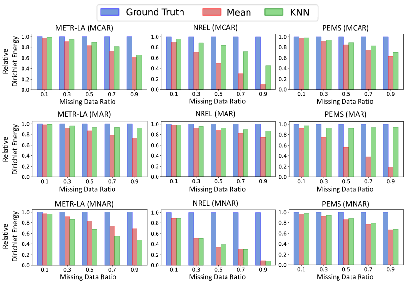
Figure 1: The Dirichlet energy of different imputation strategies on three experimental datasets (METR-LA, PEMS, NREL) with different missing ratios under three experimental missing mechanisms (MCAR, MAR, MNAR). Relative Dirichlet energy is normalized by that of the ground truth features.

3.3 Draft-then-Refine Imputation

As discussed before, the “draft-then-refine” procedure has no guarantee of maintaining Dirichlet energy. To further justify the insight, we focus on the “draft” imputation stage and find that the Dirichlet energy of the “draft” imputation matrix $\hat{\bm{X}}$ is usually less than that of the ground truth matrix $\bm{X}$.

On the theoretical side, in the following proposition, we analyze a class of imputation methods where each missing feature is filled by a convex combination of observed features from the same column.

Proposition 3.2.

Suppose each element in $\bm{X}$ is identically independent drawn from a certain distribution whose first and second moment constraints satisfy $\mathbb{E}(\bm{X}_{i,j})=0$ and $\text{Var}(\bm{X}_{i,j})=1$, and the imputation $\hat{\bm{X}}$ satisfy $\hat{\bm{X}}_{i,j}=\sum_{k\in S_{k}}\alpha_{k}\bm{X}^{\star}_{i,k}$, where $\sum_{k\in S_{k}}\alpha_{k}=1$, $\alpha_{k}\geq 0$, and $S_{k}=\{1\leq k\leq n|\bm{M}_{i,k}=1\}$, we have $\mathbb{E}[E_{D}(\hat{\bm{X}})]\leq\mathbb{E}[E_{D}(\bm{X})]$.

Proof:

We first consider the case that $\bm{X}$ only has one feature column, i.e., $\bm{X}\in\mathbb{R}^{N\times 1}$. According to Equation (1), if $\bm{X}_{i}$ and $\bm{X}_{j}$ are connected, the related term in the graph Dirichlet energy is

$$e_{D}\left(\bm{X}_{i},\bm{X}_{j}\right)=\left(\dfrac{\bm{X}_{i}}{\sqrt{1+\bm{D}_{i,i}}}-\dfrac{\bm{X}_{j}}{\sqrt{1+\bm{D}_{j,j}}}\right)^{2}.$$ (4)

Using the first and second moment constraints of $\bm{X}_{i}$ and $\bm{X}_{j}$, the expectation of $e_{D}(\bm{X}_{i},\bm{X}_{j})$ can be calculated by

$$\mathbb{E}\left(e_{D}(\bm{X}_{i},\bm{X}_{j})\right) =\text{Var}\left(\dfrac{\bm{X}_{i}}{\sqrt{1+\bm{D}_{i,i}}}\right)+\text{Var}\left(\dfrac{\bm{X}_{j}}{\sqrt{1+\bm{D}_{j,j}}}\right)$$ (5)

$$=\frac{1}{1+\bm{D}_{i,i}}+\frac{1}{1+\bm{D}_{j,j}}.$$

If $\bm{X}_{i}$ is missing and imputed by $\hat{\bm{X}}_{i}=\sum_{k\in S_{k}}\alpha_{k}\bm{X}_{k}$ while $\hat{\bm{X}_{j}}=\bm{X}_{j}$ is unchanged, we have

$$\mathbb{E}\left(e_{D}(\hat{\bm{X}}_{i},\hat{\bm{X}_{j}})\right)\leq \text{Var}\left(\dfrac{\sum_{k\in S_{k}}\alpha_{k}\bm{X}_{k}}{\sqrt{1+\bm{D}_{i,i}}}\right)+\text{Var}\left(\dfrac{\bm{X}_{j}}{\sqrt{1+\bm{D}_{j,j}}}\right)$$ (6)

$$\leq \frac{\sum_{k\in S_{k}}\alpha_{k}^{2}}{1+\bm{D}_{i,i}}+\frac{1}{1+\bm{D}_{j,j}}$$

$$\leq \frac{1}{1+\bm{D}_{i,i}}+\frac{1}{1+\bm{D}_{j,j}}.$$

On the other side, if both $\bm{X}_{i}$ and $\bm{X}_{j}$ are missing and imputed by $\hat{\bm{X}}_{i}=\sum_{k\in S_{k}}\alpha_{k}\bm{X}_{k}$ and $\hat{\bm{X}}_{j}=\sum_{k\in S_{k}}\beta_{k}\bm{X}_{k}$ respectively, we have

$$\mathbb{E}\left(e_{D}(\hat{\bm{X}}_{i},\hat{\bm{X}_{j}})\right)\leq \text{Var}\left(\dfrac{\sum_{k\in S_{k}}\alpha_{k}\bm{X}_{k}}{\sqrt{1+\bm{D}_{i,i}}}\right)+\text{Var}\left(\dfrac{\sum_{k\in S_{k}}\beta_{k}\bm{X}_{k}}{\sqrt{1+\bm{D}_{j,j}}}\right)$$ (7)

$$\leq \frac{\sum_{k\in S_{k}}\alpha_{k}^{2}}{1+\bm{D}_{i,i}}+\frac{\sum_{k\in S_{k}}\beta_{k}^{2}}{1+\bm{D}_{j,j}}$$

$$\leq \frac{1}{1+\bm{D}_{i,i}}+\frac{1}{1+\bm{D}_{j,j}}.$$

In summary, we have

$$\mathbb{E}[E_{D}(\hat{\bm{X}})]= \sum_{\{(i,j)|\bm{A}_{ij}=1\}}E(e_{D}(\hat{\bm{X}}_{i},\hat{\bm{X}_{j}}))$$ (8)

$$\leq \sum_{\{(i,j)|\bm{A}_{ij}=1\}}E(e_{D}(\bm{X}_{i},\bm{X}_{j}))$$

$$\leq \mathbb{E}[E_{D}(\bm{X})].$$

Similarly, if $\bm{X}$ has more than one feature column, i.e., $\bm{X}\in\mathbb{R}^{N\times d}$, we have $\mathbb{E}[E_{D}(\hat{\bm{X}}_{i,:})]\leq\mathbb{E}[E_{D}(\bm{X}_{i,:})]$ for $0\leq i<d$, and thus $\mathbb{E}[E_{D}(\hat{\bm{X}})]\leq\mathbb{E}[E_{D}(\bm{X})]$. ∎

Proposition 3.2 generalizes those methods that use mean, KNN, or weighted summation for the “draft” imputation and shows the universality of energy reduction. In practice, the distribution of $\bm{X}$ may not strictly follow the above assumption. Nonetheless, the reduction of Dirichlet energy still exists in the real-world imputation datasets. As shown in Figure 1, imputation strategies during the “draft” step will lead to the Dirichlet energy reduction. As the missing ratio increases, the Dirichlet energy of imputation keeps decreasing, which brings more challenges for further refinement.

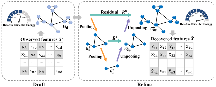
Figure 2: Overview of proposed Graph Laplacian Pyramid Network. The U-shaped autoencoder extracts the clustering and coarse patterns, while the Residual Network reconstructs local details. By combining these two parts, the model can refine the draft imputation and preserve the Dirichlet energy. The dashboards indicate the relative Dirichlet energy of draft and refined features.

4 Model Design

Inspired by the analysis above, we propose Graph Laplacian Pyramid Network (GLPN) to improve imputation performance and reduce the Dirichlet energy reduction during imputation tasks. Following the “draft-then-refine” procedure, during the first stage, we use a general method to construct the draft imputation of the missing features. During the second stage, GLPN is used to refine the node features while preserving the Dirichlet energy of the graph. Figure 2 depicts the whole framework of our model.

4.1 Draft Imputation

The model takes a missing graph $G=(\bm{X}^{\star},\bm{A})$ as input. During the first stage, we use Diffusion Graph Convolutional Networks (DGCNs) [15] to get the initial imputation of missing node features. The layer-wise propagation rule of DGCNs is expressed as:

where $\bm{D}_{O}$ and $\bm{D}_{I}$ are the out- and in-degree diagonal matrix. $M$ is the diffusion step. $\sigma$ is the activation function. $\theta\in\mathbb{R}^{M\times 2}$ is the parameters of the filter. $\bm{H}^{(k)}$ is the feature matrix after $k$-steps DGCNs. With input $\bm{H}^{(0)}=\bm{X}^{\star}$, we use $K$-layer DGCNs to get draft imputation $G_{d}=(\bm{X}_{d},\bm{A})$, where $\bm{X}_{d}=\bm{H}^{(K)}$.

4.2 GLPN Architecture

During the second stage, GLPN aims to refine the draft features for imputation. The architecture of GLPN consists of two branches: The U-shaped Autoencoder obtains coarse and hierarchical representations of the graph, while the Residual Network extracts the local details on the graph.

The U-shaped autoencoder captures the low-frequency component, which will generally lead to a low Dirichlet energy. Thus, to alleviate the Dirichlet energy decline, high-frequency components are expected. In this vein, the residual network acts as the high-pass filter to get the high-frequency component.

As shown in Figure 2, we construct a 2-level graph pyramid for illustration. $G^{l}_{p}=(\bm{X}^{l}_{p},\bm{A}_{p}^{l})$ is the reduced and clustered version of $G_{d}$ after the pooling operator at $l^{th}$ pyramid. $G^{l}_{up}=(\bm{X}^{l}_{up},\bm{A}_{up}^{l})$ denotes the $l^{th}$ level reconstructed graph after the unpooling operator. $\bm{R}^{i}$ is the detailed local information obtained via the residual network to overcome the energy decline issue. At each layer of decoder, $\bm{X}^{l}_{up}$ and $\bm{R}^{l}$ are combined and fed to the next level.

The model is trained to accurately reconstruct each feature from the observed data by minimizing the reconstruction loss:

$$\mathcal{L}=\parallel\hat{\bm{X}}-\bm{X}\parallel^{2},$$ (10)

where $\hat{\bm{X}}$ and $\bm{X}$ are the imputed and ground truth feature vectors, respectively. In the following, we will introduce the U-shaped autoencoder and residual Network in detail.

4.3 U-shaped Autoencoder

The U-shaped autoencoder aims at getting the global and clustering pattern of the graph. The encoder uses pooling operators to map the graph into the latent space. The decoder then reconstructs the entire graph from latent space by combining residuals and unpooled features.

Pooling and Unpooling: We use the self attention mechanism [26, 49] to pool the graph into coarse-grained representations. We compute the soft assignment matrix $\bm{S}^{(l)}$ as follows:

$$\bm{S}^{(l)}=\operatorname{softmax}\Big{(}\operatorname{tanh}\big{(}\bm{X}_{p}^{(l)}\bm{W}_{1}^{(l)}\big{)}\bm{W}_{2}^{(l)}\Big{)},$$ (11)

where $\bm{S}^{(l)}\in\mathbb{R}^{n_{l}\times n_{l+1}}$ donates the assignment matrix at the $l^{th}$ pooling layer, $\bm{W}_{1}^{(l)}$ and $\bm{W}_{2}^{(l)}$ are two weight matrices of the $l^{th}$ level pyramid. Then the coarsen graph structure $\bm{A}_{p}^{(l)}$ and features $\bm{X}_{p}^{(l)}$ at $l^{th}$ pyramid are

$$\bm{X}_{p}^{(l+1)}={{\bm{S}^{(l)}}^{T}}\bm{X}_{p}^{(l)};\\ ~{}\bm{A}_{p}^{(l+1)}=\operatorname{softmax}\left({\bm{S}^{(l)}}^{T}\bm{A}_{p}^{(l)}\bm{S}^{(l)}\right).$$ (12)

As for the unpooling operator, we just reverse this process and get the original size graph by

where $\oplus$ is combination operator. In the bottleneck of a $L$-level GLPN, $\bm{X}_{up}^{(L)}=\bm{X}_{p}^{(L)},\bm{A}_{up}^{(L)}=\bm{A}_{p}^{(L)}$. Given the draft imputation $\bm{X}_{p}^{(0)}=\bm{X}_{d},\bm{A}_{p}^{(0)}=\bm{A}$, we can get the final refined feature matrix $\hat{\bm{X}}=(\bm{X}_{up}^{(0)}\oplus\bm{R}^{(0)})$.

4.4 Residual Network

The goal of the residual network is to extract the high-frequency component of the graph and maintain the Dirichlet energy. We adopt Graph Deconvolutional Network (GDN) [9] which uses inverse filter $g^{-1}_{c}(\lambda_{i})=\frac{1}{1-\lambda_{i}}$ in spectral-domain to capture the detailed local information. Similar to [9], we use Maclaurin Series to approximate the inverse filter. Combining with wavelet denoising, the $M^{th}$ order polynomials of GDN can be represented as:

where $\bm{W}_{3}^{(l)}$ is the parameter set to be learned.

5 Energy Maintenance Analysis

Here, we will discuss how GLPN preserves Dirichlet energy compared with vanilla GCN [14].

5.1 Graph Convolutional Networks

First, we present the Dirichlet energy analysis of GCN. The graph filter of GCN can be represented by $\bm{P}=\bm{I}-\tilde{\Delta}$. Each layer of vanilla GCN can be written as:

$$\bm{X}^{(l+1)}=\sigma(\bm{P}\bm{X}^{(l)}\bm{W}^{(l)}).$$ (15)

After removing the non-linear activation $\sigma$ and weight matrix $\bm{W}^{(l)}$, the Dirichlet energy between neighboring layers could be represented by [50]:

$$\left(1-\lambda_{1}\right)^{2}E_{D}(\bm{X}^{(l)})\leq E_{D}(\bm{X}^{(l+1)}),$$ (16)

where $\lambda_{1}$ is the non-zero eigenvalues of matrix $\tilde{\Delta}$ that is most close to values 1. We refer to this simplified Graph Convolution [51] as simple GCN. Here, we only retain the lower bound as we focus on the perspective of energy decline.

Since the eigenvalues locate within the range $[0,2)$, $\left(1-\lambda_{1}\right)^{2}$ may be extremely close to zero, which means the lower bound of Equation (16) can be relaxed to zero. For a draft imputation $\bm{X}_{d}$, multi-layer simple GCN has no guarantee of maintaining $E_{D}(\bm{\hat{X}})$ in the refinement stage.

5.2 GLPN

Now we analyze the energy maintenance of GLPN. We use the first-order Maclaurin Series approximation of GDN (Equation (14)) to simplify the analysis, which could also be called as Laplacian Sharpening [52] with the graph filter $\bm{P}_{l}=\bm{I}+\tilde{\Delta}$.

For the proposed GLPN with one-level pooling-unpooling, the output of our model could be formulated by:

$$\hat{\bm{X}}=\bm{P}_{l}\bm{X}_{d}+\alpha\bm{S}\bm{S}^{T}\bm{X}_{d},$$ (17)

where $\bm{X}_{d}\in\mathbb{R}^{n\times d}$ is the draft imputed feature matrix of graph and $\hat{\bm{X}}$ is the refined feature. $\bm{S}\in\mathbb{R}^{n\times n_{0}}(n>n_{0})$ should be the assignment matrix and the sum of row equals to 1 (i.e. $\operatorname{sum}(\bm{S}_{i:})=1,i\in[1,n])$. The first term $\bm{P}_{l}=\bm{I}+\tilde{\Delta}$ from the residual network is used as a high-pass filter to capture the high-frequency components. The second term comes form the U-shaped autoencoder that obtains the global and low-frequency information.

Proposition 5.1.

If we use the first-order Maclaurin Series approximation of GDN as the residual layer, the Dirichlet energy of one layer simplified GLPN without the weight matrix is bounded as follows:

$$(1+C_{min})^{2}E_{D}(\bm{X}_{d})\leq E_{D}(\hat{\bm{X}}),$$ (18)

where $C_{min}$ is the minimum eigenvalue of matrix $\tilde{\Delta}+\alpha\bm{S}\bm{S}^{T}$.

Proof:

For the proposed GLPN with one-level pooling-unpooling, the output of our model could be formulated by:

$$\hat{\bm{X}}=\bm{P}_{l}\bm{X}_{d}+\alpha\bm{S}\bm{S}^{T}\bm{X}_{d}.$$ (19)

We define $\bm{Q}\triangleq\bm{P}_{l}+\alpha\bm{S}\bm{S}^{T}$, and then simplify the above expression as

$$\hat{\bm{X}}=\bm{Q}\bm{X}_{d}.$$ (20)

We represent the decomposition of matrix $\bm{Q}$ as: $\bm{Q}=\bm{U}\bm{\Lambda}\bm{U}^{T}$, where the columns of $\bm{U}$ constitute an orthonormal basis of eigenvectors of $\bm{Q}$, and the diagonal matrix $\bm{\Lambda}$ is comprised of the corresponding eigenvalues of $\bm{Q}$.

For $E_{D}(\hat{\bm{X}})$, we have:

$$\begin{split}E_{D}(\hat{\bm{X}})&=\operatorname{tr}\left((\bm{U}\bm{\Lambda}\bm{U}^{T}\bm{X}_{d})^{T}\tilde{\Delta}(\bm{U}\bm{\Lambda}\bm{U}^{T}\bm{X}_{d})\right)\\ &=\operatorname{tr}\left(\bm{X}^{T}_{d}\bm{U}\bm{\Lambda}\bm{U}^{T}\tilde{\Delta}\bm{U}\bm{\Lambda}\bm{U}^{T}\bm{X}_{d}\right)\\ &=\operatorname{tr}\left(\bm{U}^{T}\bm{X}_{d}\bm{X}^{T}_{d}\bm{U}\bm{\Lambda}\bm{U}^{T}\tilde{\Delta}\bm{U}\bm{\Lambda}\right)\\ &\geq\delta\operatorname{tr}\left(\bm{U}^{T}\bm{X}_{d}\bm{X}^{T}_{d}\bm{U}\bm{\Lambda}\bm{U}^{T}\tilde{\Delta}\bm{U}\right)\\ &=\delta\operatorname{tr}\left(\bm{\Lambda}\bm{U}^{T}\tilde{\Delta}\bm{U}\bm{U}^{T}\bm{X}_{d}\bm{X}^{T}_{d}\bm{U}\right)\\ &\geq{\delta}^{2}\operatorname{tr}\left(\bm{X}_{d}^{T}\tilde{\Delta}\bm{X}_{d}\right)\\ &={\delta}^{2}E_{D}(\bm{X}_{d}),\end{split}$$ (21)

where $\delta$ is the minimum eigenvalue of matrix $\bm{Q}$. Recalling $\bm{Q}\triangleq\bm{P}_{l}+\alpha\bm{S}\bm{S}^{T}$ and $\bm{P}_{l}\triangleq\bm{I}+\tilde{\Delta}$, then we have $\delta=1+C_{min}$, where $C_{min}$ is the minimum eigenvalue of matrix $\tilde{\Delta}+\alpha\bm{S}\bm{S}^{T}$.

In summary, we have

$$(1+C_{min})^{2}E_{D}(\bm{X}_{d})\leq E_{D}(\hat{\bm{X}}),$$ (22)

where $C_{min}$ is the minimum eigenvalue of matrix $\tilde{\Delta}+\alpha\bm{S}\bm{S}^{T}$. ∎

Except for the first-order Maclaurin Series approximation of GDN as the residual layer, we can obtain similar results in the higher-order approximation. For example, based on second-order Maclaurin Series approximation, Equation (17) would be

$$\hat{\bm{X}}=\tilde{\bm{P}}_{l}\bm{X}_{d}+\alpha\bm{S}\bm{S}^{T}\bm{X}_{d},$$ (23)

where $\tilde{\bm{P}}_{l}=\bm{I}+\tilde{\Delta}+\frac{1}{2}{\tilde{\Delta}}^{2}$. Then, we have a similar conclusion to Proposition 5.1:

$$(1+\tilde{C}_{min})^{2}E_{D}(\bm{X}_{d})\leq E_{D}(\hat{\bm{X}}),$$ (24)

where $\tilde{C}_{min}$ is the minimum eigenvalue of matrix $\tilde{\Delta}+\frac{1}{2}{\tilde{\Delta}}^{2}+\alpha\bm{S}\bm{S}^{T}$.

Meanwhile, for multi-layer GLPN, we can obtain a similar result that simplified GLPN can maintain the Dirichlet energy compared with simple GCN in Equation (16). Thus, with a non-zero bound, GLPN alleviates the decline of Dirichlet energy during the “refine” stage.

6 Experiments

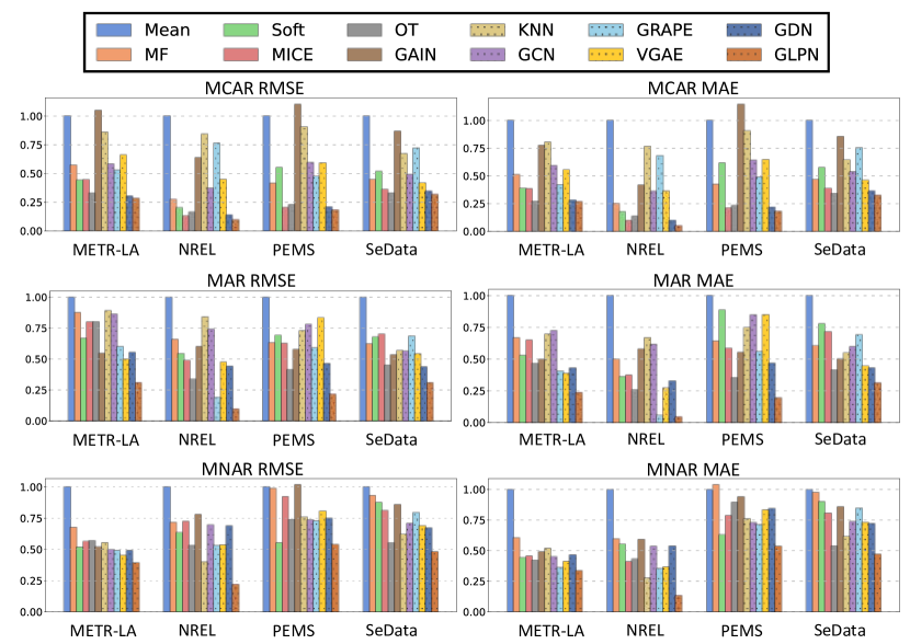
Figure 3: Imputation results on four benchmark datasets with different settings: MCAR (top), MAR (middle), and MNAR (bottom). Both RMSE (left) and MAE (right) are normalized by the performance of mean imputation.

6.1 Datasets

We conduct extensive experiments to evaluate the performance of our proposed framework on three categories of datasets: Continuous sensor datasets, Single-graph graph datasets and Multi-graph datasets. The summary of experimental datasets are shown in Table I and Table II.

• Continuous sensor datasets [11], including three traffic speed datasets, METR-LA [15], PEMS [15], SeData [53] and one solar power dataset, NREL [54]. We use a time window to generate the experimental data from the long-period time sensor data. In a system with $n$ sensors, the data collected in the length-$h$, non-overlapping time window constitutes the graph with feature matrix $\bm{X}\in\mathbb{R}^{n\times h}$. The graph structures are established by additional side information as follows. For NREL, METR-LA and PEMS, we use a thresholded Gaussian kernel applied to geographic distances following previous works [55]: We construct the adjacency matrix by $\bm{A}_{i,j}=\exp\left(-\left(\frac{\operatorname{dist}\left(v_{i},v_{j}\right)}{\sigma}\right)^{2}\right),$ where $\operatorname{dist}(v_{i},v_{j})$ represents the distance between sensor $v_{i}$ and $v_{j}$, and $\sigma$ is a normalization factor. For SeData, we construct a binary adjacency matrix defined by $\bm{A}_{i,j}=\begin{cases}1,&\text{ if }v_{i}\text{ and }v_{j}\text{ are neighbors }\\ 0,&\text{ otherwise }\end{cases}$. After a MinMax scaler [56], all the attributes can be scaled to [0,1].

  TABLE I: Summary of continuous sensor graph datasets and multi-graph datasets. The number of nodes, edges, graphs, and the number of nodes’ attributes are shown. “Cont.” means continuous data type.

  Dataset	Nodes	Edges	Features	Graphs	Data Type
  METR-LA	207	814	24	1427	Cont.
  NREL	137	269	16	2874	Cont.
  PEMS	325	1653	16	2850	Cont.
  SeData	323	1001	16	441	Cont.
  SYNTHIE	95	173	15	400	Cont.
  FRANKENSTEIN	17	18	780	4337	Cont.
  PROTEINS	39	73	29	1113	Mixed

  TABLE II: Summary of single-graph datasets. The number of nodes, edges, the number of nodes’ attributes, and the number of nodes’ classes are shown. “Homo. Ratio” indicates the homophily ratio defined by Equation (25).

  Dataset	Nodes	Edges	Features	Classes	Homo. Ratio
  Texas	183	308	1703	5	0.06
  Cornell	183	295	1703	5	0.11
  ArXiv-Year	169343	1166243	128	5	0.22
  Citeseer	2120	3679	3703	6	0.74
  Yelpchi	45954	7693958	32	2	0.77
  Cora	2485	5069	1433	7	0.81

• Single-graph datasets including three heterophilous graphs Texas, Cornell [57], ArXiv-Year [58] and three homophilous graphs Cora, Citeseer [14], YelpChi [58]. Each dataset contains only one graph. To be specific, Texas and Cornell are two web-page datasets where nodes are the web pages from computer science departments of different universities, and edges are links between pages. ArXiv-Year, Cora and Citeseer are three citation network datasets. YelpChi is a web-page hotel and restaurant review dataset.

• Multi-graph datasets including SYNTHIE [59], PROTEINS [60] and FRANKENSTEIN [61]. SYNTHIE is a synthetic dataset consisting of 400 graphs. PROTEINS is a dataset of proteins represented by mixed data: continuous features represent the length in amino acids and discrete features label the types, namely helix, sheet or loop. FRANKENSTEIN is a small molecules dataset. Each molecule is represented as a graph whose vertices are labeled by the chemical atom symbol and edges are characterized by the bond type.

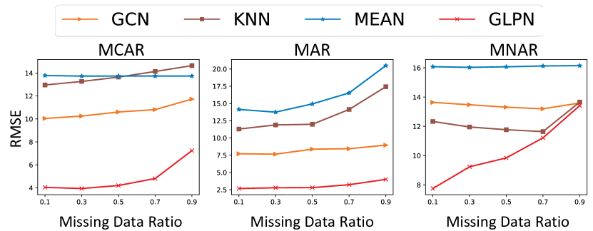
Figure 4: RMSE for METR-LA with different data missing ratios. Both structure-free and structure-based baselines are compared under three missing mechanisms.

6.2 Baselines

We compare the performance of our proposed model with the following baselines, which could be further divided into two categories: Structure-free methods and Structure-based methods. To be specific, the structure-free methods ignore the graph structure of the data, which leads to a pure matrix imputation task. On the contrary, the structure-based methods take the graph structure into consideration while performing imputation.

Structure-free methods:

• MEAN: The method imputes the missing value with the mean of all observed features.

• MF: The method uses a matrix factorization model to predict the missing values in a matrix.

• Soft [35]: SoftImpute works like EM, filling in the missing values with the current guess, and then solving the optimization problem on the complete matrix using a soft-thresholded SVD.

• MICE [6]: The method performs missing value imputation by chained equations. The procedure imputes missing data in a dataset through an iterative series of predictive models.

• OT [27]: OT assumes that two batches extracted randomly from the same dataset should share the same distribution and uses the optimal transport distances to quantify the distribution matching and impute data.

• GAIN [33]: GAIN is a Generative Adversarial Net framework to impute missing data. The generator imputes the missing components conditioned on the observed data, and the discriminator determines which components were actually observed and which were imputed.

Structure-based methods:

• KNN: The method uses the average of K-hop nearest neighbors to serve as imputed values.

• GCN [14]: The method is a basic graph convolution neural network, where each layer aggregates the features of neighbors to predict missing data.

• GRAPE [38]: The method tackles the missing data imputation problem using graph representation based on a deep learning framework.

• VGAE [62]: The method uses variational auto-encoder on graph-structured data to recover the missing data.

• GDN [9]: The method uses graph deconvolutional network to recover the missing data via an autoencoder framework.

6.3 Experimental Setup

6.3.1 Tasks and Metrics

The imputation performance will be evaluated by using three common missing data mechanisms: Missing Completely At Random (MCAR), Missing At Random (MAR), and Missing Not At Random (MNAR) [63].

MCAR refers to a missing value pattern where data points have vanished independently of other values. We generate the missingness at a rate of 20% uniformly across all the features. MAR is also a missing pattern in which values in each feature of the dataset are vanished depending on values in another feature. For MAR, we randomly generate 20% of features to have missingness caused by another disjoint subset of features. In contrast to MCAR and MAR, MNAR means that the probability of being missing depends on some unknown variables [64]. In our experiments, for MNAR, the features of some observations are entirely missing. MNAR refers to the cases of virtual sensing or interpolation, which estimates the value of observations with no available data. We use the Mean Absolute Error (MAE) and Root Mean Squared Error (RMSE) as performance metrics.

6.3.2 Parameter Settings

For all experiments, we use an 80-20 train-test split. For experimental configurations, we train our proposed model for 800 epochs using the Adam optimizer with a learning rate of 0.001. For the ”draft” imputation stage, we use a 1-layer DGCN with 100 hidden units to obtain the rudimentary imputation. We build the residual network using one GDN layer approximated by three-order Maclaurin Series. For the pooling-unpooling layer, we set the number of clusters $r$ as 60-180 according to the size of dataset, respectively.

TABLE III: The ablation study under MCAR mechanism with 20% data missing ratio. ‘w/o R’ and ‘w/o P’ mean the variants of GLPN without residual network and U-shaped autoencoder respectively.

Variant	METR-LA	NREL	PEMS	SeData
w/o R	5.345	1.121	2.565	5.963
w/o P	4.419	1.285	3.450	6.618
GLPN	4.079	0.866	1.546	3.555

TABLE IV: Imputation and classification performance on heterophilous and homophilous graphs (missing ratio = 0.8). “Full” and “Miss” represent classification results with full and missing features, respectively.

	Heterophilous graphs						Homophilous graphs
	Texas		Cornell		ArXiv-Year		Citeseer		YelpChi		Cora
	h = 0.06		h = 0.11		h=0.22		h=0.74		h=0.77		h = 0.81
	MAE	ACC(%)	MAE	ACC(%)	MAE	ACC(%)	MAE	ACC(%)	MAE	ACC(%)	MAE	ACC(%)
Full	-	55.68	-	55.95	-	44.60	-	59.36	-	63.63	-	77.20
Miss	-	49.51	-	51.12	-	41.17	-	43.64	-	61.39	-	62.47
Mean	0.0890	50.81	0.0998	52.43	0.1736	41.66	0.0166	44.07	0.3772	60.88	0.0340	62.03
KNN	0.1130	52.97	0.0899	50.97	0.1637	42.86	0.0165	45.98	0.3313	61.53	0.0302	62.17
GRAPE	0.0935	53.86	0.0955	52.73	0.1656	41.76	0.0166	44.34	0.2631	60.31	0.0281	62.76
VGAE	0.0954	53.24	0.1057	53.93	0.1698	41.47	0.0165	44.17	0.2731	61.07	0.0351	60.83
GCN	0.0833	53.77	0.0909	53.30	0.1639	42.06	0.0163	44.12	0.2665	60.75	0.0275	61.50
GDN	0.0825	54.06	0.0885	54.02	0.1595	42.12	0.0165	44.40	0.2717	59.62	0.0276	62.57
GLPN	0.0774	55.49	0.0868	54.59	0.1592	43.18	0.0157	46.06	0.2502	63.21	0.0261	63.34

6.4 Evaluation on Continuous Sensor Datasets

As shown in Figure 3, for all the three missing data mechanisms, our proposed GLPN has the best imputation performance with the lowest MAE and the lowest RMSE. Empirical results show that GLPN decreases the overall imputation error by around 9%. In general, structure-based methods (denoted by dotted bars) outperform structure-free methods (denoted by filled bars) by taking advantage of graph structure as side information. Compared with other structure-based deep learning models, such as GCN based methods, GLPN achieves the greatest performance gain thanks to the design of graph Dirichlet energy maintenance therein.

6.4.1 Robustness against Different Missing Ratios

To better understand the robustness of GLPN, we conduct the same experiments as mentioned above with different feature missing ratios varying from 0.1 to 0.9. All of the three missing mechanisms are included. Figure 4 shows the imputation performance of METR-LA dataset regarding RMSE error. Our proposed GLPN shows consistent lowest imputation errors for different data missing levels. As the missing ratio increases, GLPN maintains a fairly stable performance in both MCAR and MAR mechanisms. Although the missingness of whole observations is more challenging (under MNAR), GLPN is still able to produce satisfactory imputation for unseen observations.

6.4.2 Ablation Study

In this subsection, we investigate the influence of two branches of GLPN on imputation performance, i.e. the residual network and the pyramid autoencoder. We test the variants of GLPN without residual network (denoted by GLPN w/o R) and U-shaped autoencoder (denoted by GLPN w/o R) separately. Under MCAR mechanisms, the corresponding results (RMSE) are shown in Table III. We observe that the imputation error RMSE decreases on average 32% without residual network. Meanwhile, the U-shaped autoencoder reduces the average RMSE by 35%. By comparing the full GLPN model and two variants, it confirms that both residual network and U-shaped autoencoder branch can help improve the imputation performance.

TABLE V: Imputation Performance (MAE) on multi-graph datasets.

	SYNTHIE	PROTEINS	FRANKENSTEIN
Mean	2.239	17.925	0.4496
Soft	1.358	7.037	0.0524
Mice	1.297	3.482	0.0513
OT	2.027	9.907	0.0632
GAIN	1.664	7.003	0.0523
KNN	2.152	6.758	0.3144
GRAPE	1.579	6.236	0.0588
GCN	2.276	7.099	0.0683
GDN	1.543	6.755	0.0509
GLPN	1.209	2.812	0.0468

TABLE VI: Experiments with different draft strategies on continuous sensor dataset imputation. The table shows the RMSE normalized by the performance of mean imputation.

	METR-LA			NREL			PEMS			SeData
	MCAR	MAR	MNAR	MCAR	MAR	MNAR	MCAR	MAR	MNAR	MCAR	MAR	MNAR
Mean	1.000	1.000	1.000	1.000	1.000	1.000	1.000	1.000	1.000	1.000	1.000	1.000
Mean+GLPN	0.343	0.298	0.401	0.127	0.095	0.198	0.224	0.182	0.569	0.428	0.589	0.589
Soft	0.389	0.529	0.440	0.174	0.360	0.552	0.617	0.886	0.630	0.574	0.900	0.900
Soft+GLPN	0.233	0.204	0.584	0.076	0.085	0.223	0.188	0.188	0.695	0.324	0.670	0.670
KNN	0.805	0.697	0.521	0.764	0.667	0.275	0.905	0.751	0.758	0.645	0.617	0.617
KNN+GLPN	0.349	0.305	0.382	0.117	0.086	0.224	0.225	0.184	0.676	0.334	0.595	0.595
GCN	0.595	0.722	0.450	0.364	0.616	0.538	0.642	0.847	0.728	0.537	0.735	0.735
DGCN+GLPN	0.270	0.237	0.337	0.051	0.043	0.135	0.182	0.195	0.538	0.327	0.469	0.469

6.5 Evaluation on Heterophily Setting

Real-word graphs do not always obey the homophily assumption that similar features or same class labels are linked together. For heterophily setting, linked nodes have dissimilar features and different class labels, which cause graph signal contains more energy at high-frequency components [65]. In order to test the ability to capture both low- and high-frequency components of our model, we conduct experiments for feature imputation and node classification on different homophily ratio graphs.

Given a graph $G=\{\mathcal{V},\mathcal{E}\}$ and node label vector $y$, the node homophily ratio is defined as the average proportion of the neighbors with the same class of each node [66]:

$$h=\frac{1}{|\mathcal{V}|}\sum\limits_{v\in\mathcal{V}}\frac{|\{u\in\mathcal{N}:y_{v}=y_{u}\}|}{|\mathcal{N}(v)|}.$$ (25)

The homophily ratio $h$ of six single-graph datasets ranges from 0.06 to 0.81. We drop 80% node features through MCAR mechanism, then impute the missing data and use 1-layer GCN for downstream classification. We report MAE and average accuracy (ACC) for imputation and classification, respectively. Table IV gives detailed results.

Overall, we observe that our model has the best performance in heterophily and homophily settings. GLPN reduces MAE on imputation tasks by an average of 26% and improves accuracy on classification tasks by an average of 17% over other models. We also observe that GDN achieves competitive performance in heterophily setting. This is likely due to GDN work as a high frequency amplifier which can capture the feature distribution under heterophily. However, in homophily, neighbors are likely to have similar features, so methods follow the homophily assumption (e.g., VGAE) has better performance than GDN. Therefore, our method is able to maintain the same level of performance under heterophily and homophily settings through the design of the U-shaped autoencoder and special residual layers.

6.6 Evaluation on Multi-graph Datasets

We additionally test our model on several multi-graph datasets (i.e., SYNTHIE, PROTEINS, FRANKENSTEIN). In particular, the protein dataset, PROTEINS, is in mixed-data setting with both continuous features and discrete features.

We test our model under the MCAR mechanism with 20% missing ratio and report the imputation results in Table V. From these results, we can see that our proposed GLPN achieves the best imputation performance, which indicates that GLPN could be widely applied for different graph data imputation scenarios. Especially, for PROTEINS, GLPN is still able to beat other baseline methods in the mix-data setting.

6.7 Experiments with Different Draft Strategies

Given that the draft imputation used to start the model matters a lot, we additionally consider four draft imputation methods, including two structure-free methods (MEAN, Soft) and two structure-based methods (K-hop nearest neighbors, GCN). Note that the model described in this paper utilizes a variant of Graph Convolutional Networks (i.e. DGCN) as the draft component. We report the normalized results relative to the performance of the MEAN imputation in Table VI. Among these strategies, GCN based methods provide the best imputation performance on average. Given that the draft step is not the focus of this work, we only report the best model with DGCN drafter in the paper. It is worth noting that based on all these four draft strategies, GLPN could significantly improve the final imputation performance via an energy-preservation refine step.

6.8 Dirichlet Energy Maintenance

To validate the Dirichlet energy maintenance capability of GLPN, we compare our model with several baselines in Figure 5. The experiments are conducted on METR-LA dataset with different data missing ratios. The Dirichlet energy is normalized by the ground truth feature, which is the target of imputation. Among all the baselines, we can observe that the imputation energy of GLPN decreases the slowest with an increasing missing ratio for all three types of missing mechanisms, which also reveals the robustness of our imputation model.

To illustrate the correlation between Dirichlet energy and imputation performance, we also report the imputation performance and the relative Dirichlet energy gap between the model prediction $\bm{\hat{X}}$ and the ground truth $\bm{X}$, i.e., $\Delta E=\frac{E_{D}(\bm{\hat{X}})-E_{D}(\bm{X})}{E_{D}(\bm{X})}$ in Table VII. Among all these methods, our proposed GLPN achieves the best imputation performance as well as the least Dirichlet energy gap, consistent with the motivation of this work.

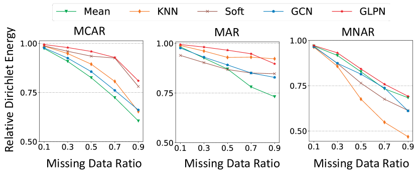
Figure 5: Relative Dirichlet energy for METR-LA imputation with different data missing ratios. The Dirichlet energy is normalized by the ground truth features, whose relative energy equals 1.

TABLE VII: Correlations between the imputation error and the Dirichlet energy gap on METR-LA dataset. $\Delta E$ denotes the relative Dirichlet energy gap.

Missing Ratio		10%	30%	50%	70%
Mean	$\Delta E$	-1.8%	-7.4%	-13.0%	-22.0%
	RMSE	14.13	13.74	14.94	16.52
KNN	$\Delta E$	-1.1%	-3.9%	-7.1%	-7.2%
	RMSE	11.29	11.89	11.98	14.13
GCN	$\Delta E$	-2.4%	-6.9%	-10.9%	-14.9%
	RMSE	7.71	7.65	8.37	8.44
GLPN	$\Delta E$	-0.7%	-1.9%	-3.5%	-5.3%
	RMSE	4.70	4.58	4.94	5.49

7 Conclusion

In this paper, we present Graph Laplacian Pyramid Network (GLPN) for missing data imputation. We initialize the first study to discuss the “draft-then-refine” imputation paradigm from the perspective of Dirichlet energy. Based on the “draft-then-refine” procedure, we develop a U-shaped autoencoder and residual network to refine the node representations based on draft imputation. We find that Dirichlet energy can be a principle to guide the design of the imputation model. We also theoretically demonstrate that our model has better energy maintenance ability. The experiments show that our model has significant improvements on several imputation tasks compared against state-of-the-art imputation approaches.

Weiqi Zhang received the B.S. degree in Industrial Engineering from Tsinghua University, Beijing, China, in 2020. She is currently pursuing the Ph.D. degree in data science and analytics, at the Hong Kong University of Science and Technology, supervised by Prof. Fugee Tsung and Prof. Jia Li. Her research interests include graph-based data mining, time series analysis and industrial big data.

Guanlve Li works as a research assistant at HKUST (Guangzhou), advised by Prof. Jia Li. She received the BS degree in communication engineering from the Southwest Jiaotong University in 2019 and the MS degree in computer science from Beijing University of Posts and Telecommunications in 2022, advised by Jinglin Li. Her research interests include graph deep learning, data mining, and computational drug design.

Jianheng Tang is a second year PhD student at HKUST, advised by Prof. Jia Li and Prof. Xiaofang Zhou. Previously, he received the MPhil degree from the Sun Yat-sen University in 2021, where he was advised by Prof. Xiaodan Liang. His research interest in general lies in graph-based data mining and knowledge-driven machine learning with real-world applications in healthcare, education, finance, etc. Some of his works have been published in ICML, ICLR, ACL, AAAI and et al.

Jia Li is an assistant professor in HKUST (Guangzhou). He received Ph.D. degree at The Chinese University of Hong Kong in 2021. Before that, he worked as a full-time data mining engineer at Tencent from 2014 to 2017, and research intern at Google AI (Mountain View) in 2020. His research interests include graph learning and data mining. Some of his works have been published in Nature Communications, TPAMI, ICML, NeurIPS, WWW, KDD and et al.

Fugee Tsung Fugee Tsung received the B.Sc. degree from National Taiwan University, Taipei, Taiwan, and the M.Sc. and Ph.D. degrees from the University of Michigan, Ann Arbor, MI, USA. He is currently a Chair Professor with Data Science and Analytics Thrust, Information Hub, the Hong Kong University of Science and Technology (Guangzhou). He is also a Chair Professor with the Department of Industrial Engineering and Decision Analytics, the Hong Kong University of Science and Technology, Hong Kong. He was the founding Acting Dean of the Information Hub at HKUST(GZ), and now serves as the Director of the Industrial Informatics and Intelligence Institute (Triple-i) and Quality and Data Analytics Lab (QLab). His research interests include quality analytics in advanced manufacturing and service processes, industrial big data, and statistical process control, monitoring, and diagnosis.

References

- [1] D. Bertsimas, C. Pawlowski, and Y. D. Zhuo, “From predictive methods to missing data imputation: an optimization approach,” The Journal of Machine Learning Research, vol. 18, no. 1, pp. 7133–7171, 2017.
- [2] M. Le Morvan, J. Josse, E. Scornet, and G. Varoquaux, “What’sa good imputation to predict with missing values?” Advances in Neural Information Processing Systems, vol. 34, 2021.
- [3] T. Kyono, Y. Zhang, A. Bellot, and M. van der Schaar, “Miracle: Causally-aware imputation via learning missing data mechanisms,” Advances in Neural Information Processing Systems, vol. 34, 2021.
- [4] K. Lakshminarayan, S. A. Harp, and T. Samad, “Imputation of missing data in industrial databases,” Applied intelligence, vol. 11, no. 3, pp. 259–275, 1999.
- [5] M. Bechny, F. Sobieczky, J. Zeindl, and L. Ehrlinger, “Missing data patterns: From theory to an application in the steel industry,” in 33rd International Conference on Scientific and Statistical Database Management, 2021, pp. 214–219.
- [6] S. Van Buuren and K. Groothuis-Oudshoorn, “mice: Multivariate imputation by chained equations in r,” Journal of statistical software, vol. 45, pp. 1–67, 2011.
- [7] K.-Y. Kim, B.-J. Kim, and G.-S. Yi, “Reuse of imputed data in microarray analysis increases imputation efficiency,” BMC bioinformatics, vol. 5, no. 1, pp. 1–9, 2004.
- [8] S. Van Buuren, “Multiple imputation of discrete and continuous data by fully conditional specification,” Statistical methods in medical research, vol. 16, no. 3, pp. 219–242, 2007.
- [9] J. Li, J. Li, Y. Liu, J. Yu, Y. Li, and H. Cheng, “Deconvolutional networks on graph data,” Advances in Neural Information Processing Systems, vol. 34, 2021.
- [10] H. Taguchi, X. Liu, and T. Murata, “Graph convolutional networks for graphs containing missing features,” Future Generation Computer Systems, vol. 117, pp. 155–168, 2021.
- [11] Y. Wu, D. Zhuang, A. Labbe, and L. Sun, “Inductive graph neural networks for spatiotemporal kriging,” in Proceedings of the AAAI Conference on Artificial Intelligence, vol. 35, no. 5, 2021, pp. 4478–4485.
- [12] S. A. Mistler and C. K. Enders, “A comparison of joint model and fully conditional specification imputation for multilevel missing data,” Journal of Educational and Behavioral Statistics, vol. 42, no. 4, pp. 432–466, 2017.
- [13] C. Cai and Y. Wang, “A note on over-smoothing for graph neural networks,” arXiv preprint arXiv:2006.13318, 2020.
- [14] T. N. Kipf and M. Welling, “Semi-supervised classification with graph convolutional networks,” in International Conference on Learning Representations, 2017.
- [15] Y. Li, R. Yu, C. Shahabi, and Y. Liu, “Diffusion convolutional recurrent neural network: Data-driven traffic forecasting,” in International Conference on Learning Representations, 2018.
- [16] W. Huang, Y. Rong, T. Xu, F. Sun, and J. Huang, “Tackling over-smoothing for general graph convolutional networks,” arXiv preprint arXiv:2008.09864, 2020.
- [17] Y. Min, F. Wenkel, and G. Wolf, “Scattering gcn: Overcoming oversmoothness in graph convolutional networks,” Advances in Neural Information Processing Systems, vol. 33, pp. 14 498–14 508, 2020.
- [18] O. Troyanskaya, M. Cantor, G. Sherlock, P. Brown, T. Hastie, R. Tibshirani, D. Botstein, and R. B. Altman, “Missing value estimation methods for dna microarrays,” Bioinformatics, vol. 17, no. 6, pp. 520–525, 2001.
- [19] A. Sportisse, C. Boyer, and J. Josse, “Estimation and imputation in probabilistic principal component analysis with missing not at random data,” Advances in Neural Information Processing Systems, vol. 33, pp. 7067–7077, 2020.
- [20] V. Audigier, F. Husson, and J. Josse, “Multiple imputation for continuous variables using a bayesian principal component analysis,” Journal of statistical computation and simulation, vol. 86, no. 11, pp. 2140–2156, 2016.
- [21] S. Bose, C. Das, T. Gangopadhyay, and S. Chattopadhyay, “A modified local least squares-based missing value estimation method in microarray gene expression data,” in 2013 2nd International Conference on Advanced Computing, Networking and Security. IEEE, 2013, pp. 18–23.
- [22] P. Keerin and T. Boongoen, “Improved knn imputation for missing values in gene expression data,” Computers, Materials and Continua, vol. 70, no. 2, pp. 4009–4025, 2021.
- [23] S. Luan, C. Hua, Q. Lu, J. Zhu, M. Zhao, S. Zhang, X.-W. Chang, and D. Precup, “Revisiting heterophily for graph neural networks,” in Advances in Neural Information Processing Systems, 2022.
- [24] H. De Silva and A. S. Perera, “Missing data imputation using evolutionary k-nearest neighbor algorithm for gene expression data,” in 2016 Sixteenth International Conference on Advances in ICT for Emerging Regions (ICTer). IEEE, 2016, pp. 141–146.
- [25] E. Rossi, H. Kenlay, M. I. Gorinova, B. P. Chamberlain, X. Dong, and M. Bronstein, “On the unreasonable effectiveness of feature propagation in learning on graphs with missing node features,” arXiv preprint arXiv:2111.12128, 2021.
- [26] J. Lee, I. Lee, and J. Kang, “Self-attention graph pooling,” in International conference on machine learning. PMLR, 2019, pp. 3734–3743.
- [27] B. Muzellec, J. Josse, C. Boyer, and M. Cuturi, “Missing data imputation using optimal transport,” in International Conference on Machine Learning. PMLR, 2020, pp. 7130–7140.
- [28] P. J. García-Laencina, J.-L. Sancho-Gómez, and A. R. Figueiras-Vidal, “Pattern classification with missing data: a review,” Neural Computing and Applications, vol. 19, no. 2, pp. 263–282, 2010.
- [29] A. P. Dempster, N. M. Laird, and D. B. Rubin, “Maximum likelihood from incomplete data via the em algorithm,” Journal of the Royal Statistical Society: Series B (Methodological), vol. 39, no. 1, pp. 1–22, 1977.
- [30] L. Gondara and K. Wang, “Mida: Multiple imputation using denoising autoencoders,” in Pacific-Asia conference on knowledge discovery and data mining. Springer, 2018, pp. 260–272.
- [31] P.-A. Mattei and J. Frellsen, “Miwae: Deep generative modelling and imputation of incomplete data sets,” in International conference on machine learning. PMLR, 2019, pp. 4413–4423.
- [32] O. Ivanov, M. Figurnov, and D. Vetrov, “Variational autoencoder with arbitrary conditioning,” in 7th International Conference on Learning Representations, ICLR 2019, 2019.
- [33] J. Yoon, J. Jordon, and M. Schaar, “Gain: Missing data imputation using generative adversarial nets,” in International conference on machine learning. PMLR, 2018, pp. 5689–5698.
- [34] J.-F. Cai, E. J. Candès, and Z. Shen, “A singular value thresholding algorithm for matrix completion,” SIAM Journal on optimization, vol. 20, no. 4, pp. 1956–1982, 2010.
- [35] T. Hastie, R. Mazumder, J. D. Lee, and R. Zadeh, “Matrix completion and low-rank svd via fast alternating least squares,” The Journal of Machine Learning Research, vol. 16, no. 1, pp. 3367–3402, 2015.
- [36] R. Mazumder, T. Hastie, and R. Tibshirani, “Spectral regularization algorithms for learning large incomplete matrices,” The Journal of Machine Learning Research, vol. 11, pp. 2287–2322, 2010.
- [37] D. J. Stekhoven and P. Bühlmann, “Missforest—non-parametric missing value imputation for mixed-type data,” Bioinformatics, 2012.
- [38] J. You, X. Ma, Y. Ding, M. J. Kochenderfer, and J. Leskovec, “Handling missing data with graph representation learning,” Advances in Neural Information Processing Systems, vol. 33, pp. 19 075–19 087, 2020.
- [39] T. Emmanuel, T. M. Maupong, D. Mpoeleng, T. Semong, B. Mphago, and O. Tabona, “A survey on missing data in machine learning,” J. Big Data, vol. 8, no. 1, p. 140, 2021.
- [40] O. G. Troyanskaya, M. N. Cantor, G. Sherlock, P. O. Brown, T. Hastie, R. Tibshirani, D. Botstein, and R. B. Altman, “Missing value estimation methods for DNA microarrays,” Bioinform., vol. 17, no. 6, pp. 520–525, 2001.
- [41] S. Bose, C. Das, T. Gangopadhyay, and S. Chattopadhyay, “A modified local least squares-based missing value estimation method in microarray gene expression data,” in 2013 2nd International Conference on Advanced Computing, Networking and Security, Mangalore, India, December 15-17, 2013. IEEE, 2013, pp. 18–23.
- [42] P. J. Burt and E. H. Adelson, “The laplacian pyramid as a compact image code,” in Readings in computer vision. Elsevier, 1987, pp. 671–679.
- [43] W.-S. Lai, J.-B. Huang, N. Ahuja, and M.-H. Yang, “Deep laplacian pyramid networks for fast and accurate super-resolution,” in Proceedings of the IEEE conference on computer vision and pattern recognition, 2017, pp. 624–632.
- [44] W.-S. Lai, J.-B. Huang, N. Ahuja, and M.-H. Yang, “Fast and accurate image super-resolution with deep laplacian pyramid networks,” IEEE transactions on pattern analysis and machine intelligence, vol. 41, no. 11, pp. 2599–2613, 2018.
- [45] S. Anwar and N. Barnes, “Densely residual laplacian super-resolution,” IEEE Transactions on Pattern Analysis and Machine Intelligence, vol. 44, no. 3, pp. 1192–1204, 2020.
- [46] H. Gao and S. Ji, “Graph u-nets,” in international conference on machine learning. PMLR, 2019, pp. 2083–2092.
- [47] N. Rabin and D. Fishelov, “Missing data completion using diffusion maps and laplacian pyramids,” in International Conference on Computational Science and Its Applications. Springer, 2017, pp. 284–297.
- [48] N. Rabin and D. Fishelov, “Two directional laplacian pyramids with application to data imputation,” Advances in Computational Mathematics, vol. 45, no. 4, pp. 2123–2146, 2019.
- [49] J. Li, Y. Rong, H. Cheng, H. Meng, W. Huang, and J. Huang, “Semi-supervised graph classification: A hierarchical graph perspective,” in The World Wide Web Conference, 2019, pp. 972–982.
- [50] K. Zhou, X. Huang, D. Zha, R. Chen, L. Li, S.-H. Choi, and X. Hu, “Dirichlet energy constrained learning for deep graph neural networks,” Advances in Neural Information Processing Systems, vol. 34, 2021.
- [51] F. Wu, A. Souza, T. Zhang, C. Fifty, T. Yu, and K. Weinberger, “Simplifying graph convolutional networks,” in International conference on machine learning. PMLR, 2019, pp. 6861–6871.
- [52] J. Park, M. Lee, H. J. Chang, K. Lee, and J. Y. Choi, “Symmetric graph convolutional autoencoder for unsupervised graph representation learning,” in Proceedings of the IEEE/CVF International Conference on Computer Vision, 2019, pp. 6519–6528.
- [53] Z. Cui, R. Ke, and Y. Wang, “Deep bidirectional and unidirectional lstm recurrent neural network for network-wide traffic speed prediction,” arXiv preprint arXiv:1801.02143, 2018.
- [54] Z. Cui, K. Henrickson, R. Ke, and Y. Wang, “Traffic graph convolutional recurrent neural network: A deep learning framework for network-scale traffic learning and forecasting,” IEEE Transactions on Intelligent Transportation Systems, 2019.
- [55] A. Cini, I. Marisca, and C. Alippi, “Filling the g_ap_s: Multivariate time series imputation by graph neural networks,” in International Conference on Learning Representations, 2021.
- [56] A. Rajaraman and J. D. Ullman, Mining of massive datasets. Cambridge University Press, 2011.
- [57] A. P. García-Plaza, V. Fresno, R. M. Unanue, and A. Zubiaga, “Using fuzzy logic to leverage html markup for web page representation,” IEEE Transactions on Fuzzy Systems, vol. 25, no. 4, pp. 919–933, 2016.
- [58] D. Lim, F. Hohne, X. Li, S. L. Huang, V. Gupta, O. Bhalerao, and S. N. Lim, “Large scale learning on non-homophilous graphs: New benchmarks and strong simple methods,” Advances in Neural Information Processing Systems, vol. 34, pp. 20 887–20 902, 2021.
- [59] C. Morris, N. M. Kriege, K. Kersting, and P. Mutzel, “Faster kernels for graphs with continuous attributes via hashing,” in 2016 IEEE 16th International Conference on Data Mining (ICDM). IEEE, 2016, pp. 1095–1100.
- [60] K. M. Borgwardt, C. S. Ong, S. Schönauer, S. Vishwanathan, A. J. Smola, and H.-P. Kriegel, “Protein function prediction via graph kernels,” Bioinformatics, vol. 21, no. suppl_1, pp. i47–i56, 2005.
- [61] F. Orsini, P. Frasconi, and L. De Raedt, “Graph invariant kernels,” in Twenty-Fourth International Joint Conference on Artificial Intelligence, 2015.
- [62] T. N. Kipf and M. Welling, “Variational graph auto-encoders,” arXiv preprint arXiv:1611.07308, 2016.
- [63] D. B. Rubin, “Inference and missing data,” Biometrika, vol. 63, no. 3, pp. 581–592, 1976.
- [64] K. Mohan, J. Pearl, and J. Tian, “Graphical models for inference with missing data,” Advances in neural information processing systems, vol. 26, 2013.
- [65] J. Zhu, Y. Yan, L. Zhao, M. Heimann, L. Akoglu, and D. Koutra, “Beyond homophily in graph neural networks: Current limitations and effective designs,” Advances in Neural Information Processing Systems, vol. 33, pp. 7793–7804, 2020.
- [66] X. Zheng, Y. Liu, S. Pan, M. Zhang, D. Jin, and P. S. Yu, “Graph neural networks for graphs with heterophily: A survey,” arXiv preprint arXiv:2202.07082, 2022.