PITT-PACC-2311 Nanosecond anomaly detection with decision trees for high energy physics and real-time application to exotic Higgs decays

Abstract

We present a novel implementation of the artificial intelligence autoencoding algorithm, used as an ultrafast and ultraefficient anomaly detector, built with a forest of deep decision trees on FPGA, field programmable gate arrays. Scenarios at the Large Hadron Collider at CERN are considered, for which the autoencoder is trained using known physical processes of the Standard Model. The design is then deployed in real-time trigger systems for anomaly detection of new unknown physical processes, such as the detection of exotic Higgs decays, on events that fail conventional threshold-based algorithms. The inference is made within a latency value of $25\,\textrm{ns}$, the time between successive collisions at the Large Hadron Collider, at percent-level resource usage. Our method offers anomaly detection at the lowest latency values for edge AI users with tight resource constraints.

Keywords: Data processing methods, Data reduction methods, Digital electronic circuits, Trigger algorithms, and Trigger concepts and systems (hardware and software).

1 Introduction

Unsupervised artificial intelligence (AI) algorithms enable signal-agnostic searches for beyond the Standard Model (BSM) physics at the Large Hadron Collider (LHC) at CERN [1]. The LHC is the highest energy proton and heavy ion collider that is designed to discover the Higgs boson [2, 3] and study its properties [4, 5] as well as to probe the unknown and undiscovered BSM physics (see, e.g., [6, 7, 8]). An active area of AI research in high energy physics is in using autoencoders for anomaly detection, much of which provides methods to find unanticipated BSM physics. Much of the existing literature, mostly using neural network-based approaches, focuses on identifying BSM physics in already collected data [9, 10, 11, 12, 13, 14, 15, 16, 17, 18, 19, 20, 21, 22, 23, 24, 25, 26, 27, 28, 29, 30, 37, 31, 32, 33, 34, 35, 36, 38, 39, 40, 41, 42, 43, 44, 45, 46, 47, 48, 49, 50, 51, 52, 53, 55, 54, 56, 57, 58, 59, 60, 61, 62, 63]. Such ideas have started to produce experimental results on the analysis of data collected at the LHC [64, 65, 66]. A related, but separate endeavor, which is the subject of this paper, is enabling the identification of anomalous data on the real-time trigger path for further investigation.

The LHC offers an environment with an abundance of data at a $40\,\textrm{MHz}$ collision rate, corresponding to the $25\,\textrm{ns}$ time period between successive collisions. The real-time trigger path of the ATLAS and CMS experiments [67, 68], e.g., processes data at a $40\,\textrm{MHz}$ input rate using custom electronics using field programmable gate arrays (FPGA) followed by software trigger algorithms executed on a computing farm. The first-level FPGA portion of the trigger system accepts between $100$ to $1000\,\textrm{kHz}$ of collisions, discarding the remaining $\approx 99\%$ of the collisions. Therefore, it is essential for new physics discovery that the FPGA-based trigger system is capable of detecting potential BSM events. A previous study aimed for LHC data has shown that an anomaly detector based on neural networks can be implemented on FPGA with latency values between $80$ to $1480\,\textrm{ns}$, depending on the design [69].

In this paper, we present a novel implementation of an autoencoder using deep decision trees that makes inferences in $25\,\textrm{ns}$. As discussed previously [70, 71], decision tree designs depend only on threshold comparisons resulting in ultrafast and ultraefficient FPGA implementation with minimal reliance on digital signal processors. We train the autoencoder on known Standard Model (SM) processes to help identify unknown and undiscovered BSM processes.

Our benchmark physics process is to search for Higgs bosons decaying to a pair of BSM pseudoscalars to leptonic final states, one of the so-called exotic Higgs decays [72], that fail the conventional threshold-based single-lepton trigger algorithms. The requirement demonstrates our method’s ability to save BSM physics events that would otherwise be discarded with the existing approach. As a separate test case, we consider an additional dataset with a range of different BSM models, referred to here as the LHC physics dataset [73] to compare to existing results. Lastly, the robustness of our general method is considered by training with samples having varying levels of signal contamination.

This paper uses Higgs bosons to explore the unknown using real-time computing. But more generally, such inferences made on edge AI may be of interest in other experimental setups and situations with tight resource constraints and latency requirements.

2 Method

Our autoencoder (AE) is related to, and extends beyond, those based on random forests [74, 75]. We note that there are related concepts in the literature with various level of algorithmic sophistication [76, 77, 78, 79], but these approaches may be more challenging to implement on the FPGA. We build on the deep decision tree architecture that uses parallel decision paths of fwXmachina [70, 71]. A general discussion of the tree-based autoencoder is given below. The subsections that follow will detail the ML training, the firmware design, including verification and validation, and the simulation samples.

A tree of maximum depth $D$ takes an input vector $\mathbf{x}$, encodes it to the latent space as $\mathbf{w}$, then decodes $\mathbf{w}$ to an output vector $\hat{\mathbf{x}}$. Typically both $\mathbf{x}$ and $\hat{\mathbf{x}}$ are elements of $\mathbb{R}^{V}$ while $\mathbf{w}$ is an element of $\mathbb{R}^{T}$, where $V$ is the number of input variables and $T$ is the number of trees, i.e.,

$$\mathbf{x}\quad\overbrace{\xrightarrow{\textrm{encoder}}\quad\mathbf{w}\quad\xrightarrow{\textrm{decoder}}}^{\textrm{autoencoder}}\quad\hat{\mathbf{x}}.$$ (1)

Typically the latent space is smaller than the input-output space, i.e., $T<V$, but it is not a requirement. A decision tree divides up the input space $\mathbb{R}^{V}$ into a set of partitions $\{P_{b}\}$ labeled by bin number $b$. The $b$ is a $B$-bit integer, where $B\leq 2^{D}$, since the tree is a sequence of binary splits.

The encoding occurs when the decision tree processes an input vector $\mathbf{x}$ to place it into a one of the partitions labeled by $w$. If more than one tree is used, then $w$ generalizes to a vector $\mathbf{w}$. The decoding occurs when $\mathbf{w}$ produces $\hat{\mathbf{x}}$ using the same forest. The bin number $b$ corresponds to a partition in $\mathbb{R}^{V}$, which is a hyperrectangle $P_{b}$ defined by a set of extrema in $V$ dimensions.

A metric $d$ provides an anomaly score calculated as a distance between the input and output, $\Delta{\,=\,}d(\mathbf{x},\hat{\mathbf{x}})$. Our choice for the estimator of $P_{b}$ is the dimension-wise central tendency of the training data sample in the considered bin, $\hat{\mathbf{x}}{\,=\,}\textrm{median}(\{\mathbf{x}\})\ \forall\ \mathbf{x}{\,\in\,}P_{b}$. The median minimizes the $L^{1}$ norm, or Manhattan distance, with respect to input data resembling the training sample.

The encoding and decoding are conceptually two steps, with the latent space separating the two. But, as explained in the next section, our design executes both steps simultaneously and bypasses the latent space altogether by a process we call $\star$coder (star-coder), i.e., $\hat{\textbf{x}}=\star\textbf{x}$,

$$\mathbf{x}~{}~{}\xrightarrow{~{}\textrm{$\star$coder}~{}}~{}~{}\hat{\mathbf{x}}.$$ (2)

Finally, the anomaly score is the sum of the $L^{1}$ distances for each tree in the forest, i.e.,

$$\Delta(\mathbf{x})=d(\mathbf{x},\star\mathbf{x})=\sum_{\begin{subarray}{c}\textrm{trees}\\ t\end{subarray}}\sum_{\begin{subarray}{c}\textrm{vars}\phantom{t}\!\!\\ v\phantom{t}\!\!\end{subarray}}\left|x_{v}-\star{x}_{v,t}\right|.$$ (3)

When the parameters of the AE are trained on known SM events, the autoencoder ideally produces a relatively small $\Delta$ when it encounters an SM event and a relatively large $\Delta$ when it encounters a BSM event.

An illustrative example of the decision tree structure is given in Supplemental Fig. A.1 and a demonstration of the autoencoder using the mnist dataset [80] is given in Supplemental Fig. A.2.

2.1 ML training

The machine learning (ML) training of the autoencoder described here is novel and is suitable for the physics problems at hand. Qualitatively, the training puts small-sized bins around regions with high event density and large-sized bins around regions of sparse event density. An illustration of the bin sizes is given with a 2d toy example in Supplemental Fig. A.3.

The following steps are executed: (1) Start with the training sample $S$ for $s$ in steps 2–4 and depth $d=1$. (2) For the sample $s$, the PDF $p_{v}$ is the marginal distributions of bit-integer-valued input variables $x_{v}\in\mathbf{x}$. The PDF $p_{m}$ is the distribution of the maximum values of the set $\{p_{v}\,\forall\,v\in V\}$. Sampling $p_{m}$ yields $\tilde{m}=m_{\tilde{v}}$ that corresponds to the $x_{\tilde{v}}$. (3) The PDF $p_{\tilde{v}}$ is for the $x_{\tilde{v}}$ under consideration. Sampling $p_{\tilde{v}}$ yields a threshold value $\tilde{c}$. (4) The sample $s$ is split by a cut $g=(x_{\tilde{v}}<\tilde{c})$. (5) The steps 2–4 are continued recursively for the two subsamples until one of two stopping conditions are met: (i) the number of splits exceeds the maximum allowed depth $D$, (ii) the split in step 3 produces a sample that is below the smallest allowed fraction $f$ of $S$. (6) When stopped, the procedure breaks out of the recursion by appending the requirement $g$ to the set $G$. (7) In the end, the algorithm produces a partition $G$ of the training sample called the decision tree grid (DTG) that corresponds to a deep decision tree (DDT) illustrated in Fig. 1. The pseudocode given below finds $G=\textrm{DTG}(S,\emptyset,1)$.

0.35

0:  $\textrm{DTG}(\textrm{training~{}sample~{}}s,\textrm{partition~{}}G,\textrm{depth}~{}d)$

1:  if $|s|/|S|<f~{}\textbf{or}{}~{}d>D$ then

2:     return  $G$

3:  end ifIdentify the variable $x_{\tilde{v}}$ to cut on

4:  $p_{v}\leftarrow\textrm{PDF}(x_{v})\ \forall~{}x_{v}{\,\in\,}\mathbf{x}$  Build set of pdfs for input variables

5:  $p_{m}\leftarrow\textrm{PDF}(\{\max(p_{v})\}\ \forall~{}v{\,\in\,}V)$  Build pdf of max of input pdfs

6:  $\tilde{m}\leftarrow\textrm{sample}(p_{m})$  Sample max

7:  $\tilde{v}\leftarrow v\ \textrm{where}\ m_{v}=\tilde{m}$  Find variable index Find threshold $\tilde{t}$ to cut on $x_{\tilde{v}}$

8:  $\tilde{c}\leftarrow\textrm{sample}(p_{\tilde{v}})$  Sample variable

9:  $g\leftarrow x_{\tilde{v}}<\tilde{c}$  Make selection Build partition

10:  $G\leftarrow\textrm{append~{}}g$  Add to $G$ the new selection $g$ Recursively build the decision tree

11:  call $\textrm{DTG}(s\textbf{~{}if~{}}g,g,d+1)$  Call DTG on subset passing $g$

12:  call $\textrm{DTG}(s\textbf{~{}if~{}}\textbf{not}{}\,g,\textbf{not}{}\,g,d+1)$  Call DTG on subset failing $g$

13:  return  $G$

Weighted randomness in both variable selection $x_{\tilde{v}}$ and threshold selection $\tilde{c}$ allow for the construction of a forest of non-identical decision trees to provide better accuracy in the aggregate. As our ML training is agnostic to the signal process, the so-called boost weights cannot be computed.

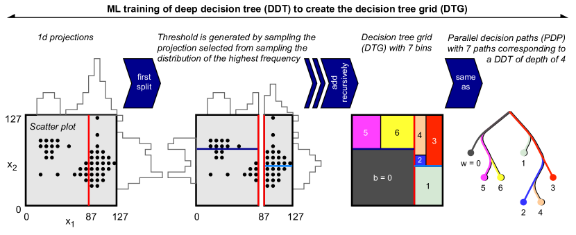
Figure 1: Illustration of the ML training. Data is represented as $x_{1}$ vs. $x_{2}$ (leftmost). Recursive importance sampling considers the marginalized distributions (second). A decision tree grid is constructed (third). Deep decision trees with maximum depth of $4$ corresponds to parallel decision paths (rightmost).

2.2 Firmware design

The structure of the firmware is based on fwXmachina [70, 71]. The Autoencoder Processor, whose block diagram is shown in Fig. 2, takes in input data and outputs the anomaly score. In the firmware implementation, we approximate $\mathbb{R}$ of the input-output space by $N$-bit integers $\mathbb{Z}_{N}$.

In the diagram, input enters from the left and copies are distributed to $T$ deep decision trees, each tree corresponding to one latent dimension. Once the outputs of the engine are available, the distance processor computes the $\Delta$ with respect to the input. The Deep Decision Tree Engine (DDTE) [71] is modified to output a vector of values. The Distance Processor takes the outputs of DDTE and computes the distance for each set of outputs followed by a sum.

We note that further modification of DDTE would allow for efficient transmission of compressed data [81], but is beyond the scope of this paper.

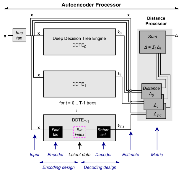
Figure 2: Block diagram of the Autoencoder Processor for anomaly detection with a $T$-dimensional latent layer corresponding to a forest of $T$ decision trees. The design uses Deep Decision Tree Engine [71], as both encoder and decoder with the bin index shown only schematically, as the latent data is implicit.

Verification and validation

We validate and verify our design using the benchmark physics scenario of Sec. 3.1.

For validation of our algorithm, first we run $\mathcal{O}(10^{5})$ test vectors through our design using C simulation in Vivado HLS and compare the outputs to that of the expected firmware outputs simulated in Python. Then co-simulation is done, which creates an RTL model of the design, simulates it, and compares the RTL model against the C design. In all cases, the simulation outputs match the expected outputs.

For the physical verification of our algorithm, we program select configurations onto the Xilinx Virtex UltraScale+ FPGA VCU118 Evaluation Kit at a clock speed of 320 MHz, which is the setup used for the benchmark results in this paper. We test a handful of test vector inputs and use the Xilinx Integrated Logic Analyzer IP core to observe the outputs. In all cases, the outputs match the expected outputs received from software and co-simulation.

2.3 Simulated samples

Samples of the multistage process of simulating the proton collisions that produce our final state followed by the simulation of the detector effects, so called Monte Carlo samples, are considered in order to test the autoencoder’s performance in real-time triggers.

We produced a sample of simulated proton-proton collision events in the SM composed of all processes that produce the $e^{+}e^{-}\mu^{+}\mu^{-}$ final state, which we consider the background process. This background is dominated by the $ZZ^{\ast}\rightarrow e^{+}e^{-}\mu^{+}\mu^{-}$ process.

Additionally, two signal samples that simulate the production and decay of scalar bosons are generated, which we consider the anomaly processes. The samples are inspired by and similar to a previous study [63]. In particular, we consider the decays of the Higgs boson ($H_{125}$) with a mass of $125\,\textrm{GeV}$ and a BSM scalar ($H_{70}$) with a mass of $70\,\textrm{GeV}$, produced in the same way as the $H_{125}$. For each scenario, the $H$ decays to a pair of BSM pseudoscalars $aa^{\prime}$ that decay to charged leptons [63]. Scalar bosons produced from the gluon-gluon fusion (ggF) production mode in proton-proton collisions are decayed as $H_{70}\rightarrow a_{25}a_{30}$ and $H_{125}\rightarrow a_{10}a_{15}$. The lighter $a$ decays to $e^{+}e^{-}$ and the heavier $a$ decays to $\mu^{+}\mu^{-}$. All samples, both background and anomaly, use the Higgs effective field theory (HEFT) model in MadGraph5$\_$aMC 2.9.5 [82].

The input variables are the three invariant masses of the $ee$, $\mu\mu$, and $ee\mu\mu$ subsystems, similar to the design of Ref. [63]. All samples are produced with the above-mentioned MadGraph5 and decayed and showered with Pythia8 [83]. Detector simulation and event reconstruction is simulated with Delphes 3.5.0 [84, 85]. A mean number of 50 simultaneous proton-proton interactions (pileup) are simulated in each collision [86]. The Delphes step uses the CMS with pileup card to simulate the behavior of the CMS detector [87]. More details can be found with the samples [90]. The input variable distributions are given in Fig. 3.

In order to simulate a scenario in which our anomaly detector would benefit a real-time trigger, e.g., at the ATLAS Level-0 / Level-1 real-time trigger system at the HL-LHC, we exclude events (from both training and evaluation) that would pass a single-lepton $p_{\textrm{T}}{\,>\,}23\,\textrm{GeV}$ cut. By doing so, we show the unique potential of our design to save BSM events that would not currently pass the real-time trigger.

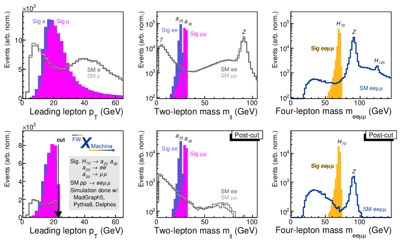
Figure 3: Input variable distributions for $H_{70}\rightarrow{a}_{25}{a}_{30}\rightarrow e^{+}e^{-}\mu^{+}\mu^{-}$ and SM to $e^{+}e^{-}\mu^{+}\mu^{-}$. Plots are given for leading lepton (left column), two-lepton (middle), and four-lepton (right) subsystems per event. Distributions are given for all events (top row) and for the events failing the single-lepton trigger with the $p_{\textrm{T}}$ threshold of $23\,$GeV for $e$ and $\mu$ (bottom). Background distributions are considered to be all Standard Model processes that result in the $e^{+}e^{-}\mu^{+}\mu^{-}$ final state, including the $H_{125}$. Prior to the one-lepton $p_{\textrm{T}}$ cut (top row), the small contribution in the SM distribution at $m_{ee\mu\mu}=125\,$GeV is visible due to $H_{125}\rightarrow ZZ^{\ast}\rightarrow e^{+}e^{-}\mu^{+}\mu^{-}$. The relative normalization between signal and background samples are arbitrary, but the normalization within the different processes in the background sample, including the $H_{125}$, are according to simulation of the Standard Model.

3 Results

We present our benchmark results of a realistic scenario in which an anomaly detector could discover BSM exotic Higgs decays with detection at the real-time trigger path. As a test case, we also consider the LHC physics dataset [73]. Our results are compared to the neural network implementation [69]. Lastly, a study showing our autoencoder’s effectiveness to signal contamination of training data is presented.

3.1 Benchmark scenario: Exotic Higgs decays

A forest of 40 decision trees was trained at a maximum depth of 5 on a training subset of SM background and applied to both a testing subset of the SM background and two signal samples. Anomaly scores for each event are calculated and are shown in the top-left figure of Fig. 4; the ROC curve is shown on the top-right figure. The AE applied to the signal $H_{125}\rightarrow a_{15}a_{10}$ achieves about $90\%$ signal efficiency with sub-percent-level SM acceptance. The AE applied to the signal $H_{70}\rightarrow a_{25}a_{30}$ achieves about $90\%$ signal efficiency at ten-percent-level SM acceptance. However, we note that the SM acceptance plateaus at the $10\%$ level because the signal distribution peaks on top of a smoothly falling SM background distribution.

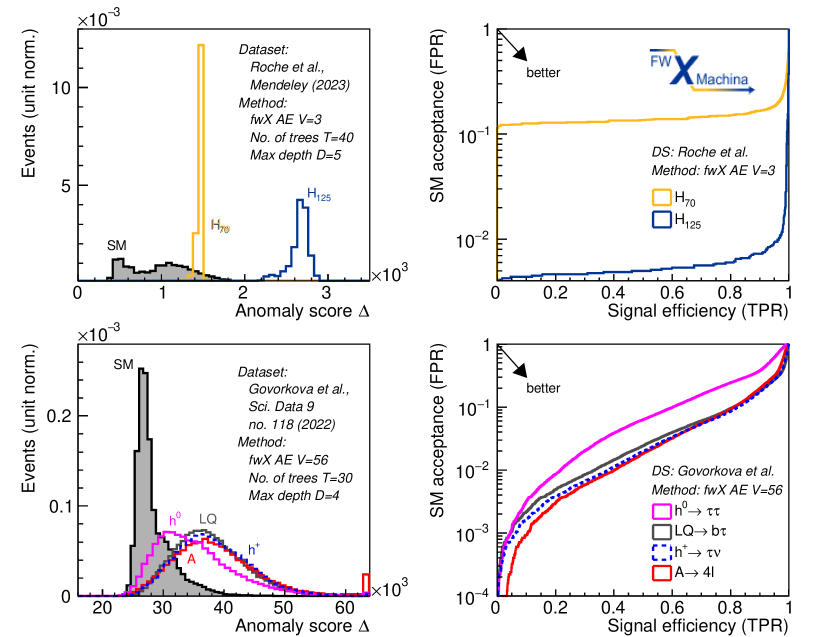
Figure 4: Physics performance results. The distribution are given for anomaly scores $\Delta$ (left column) and the ROC curves are shown (right column) for the $H\rightarrow aa^{\prime}\rightarrow e^{+}e^{-}\mu^{+}\mu^{-}$ scenario (top row) and the LHC physics dataset [73] (bottom row). The autoencoder is trained only on the respective Standard Model processes. TPR and FPR represent true and false positive rates, respectively. The plots are software-simulated results using bit integers as done in the firmware.

For the FPGA cost, the configuration is run on an xcvu9p FPGA with a clock speed of $320\,\textrm{MHz}$. Algorithm latency is 8 clock ticks (25 ns) and the interval is 1 clock tick (3.125 ns). About $3\%$ of available look up tables (LUT) are used; less than $1\%$ of flip flops (FF) are used; a negligible number of digital signal processors (DSP) is used; no BRAM or URAM is used. The results are summarized in the first column of Table 1.

For models with resonances, such as the $H_{70}$ above, it may be possible to implement a real-time window selection requirement on the anomaly score to select only the anomaly process, e.g, $1400<\Delta<1500$. In practice, this could be done by analyzing data collected with other triggers, or in real-time, by processing large numbers of events to generate a distribution on a processor near the FPGA, e.g., System on Chip (SoC) like the Zynq system considered as a cross-check for the LHC physics scenario considered in the next section.

Table 1: FPGA specifications and cost results. The first column describes the design for $e^{+}e^{-}\mu^{+}\mu^{-}$; see text details for the signal models on which the design is tested. The second column compares our results for the problem in the third column [69]. For the third column, the results listed are for DNN VAE PTQ 8-bit and CNN AE QAT 4-bit, representing the range of reported outcomes; the ^∗ indicates that the numbers are found using the published percentages.

	This paper		This paper		Govorkova et al. [69]
ML training and setup
Framework	fwXmachina		fwXmachina		hls4ml
Dataset	$e^{+}e^{-}\mu^{+}\mu^{-}$		[73]		[73]
Input variables	3		56		56
No. of trees $T$	40		30		NA since uses neural networks
Max. depth $D$	5		4		NA since uses neural networks
Phys. performance	-		Comparable to [69]		[69]
FPGA and firmware setup
Chip family	Xilinx Virtex US+		Xilinx Virtex US+		Xilinx Virtex UltraScale+
Chip model	xcvu9p-flga2104-2L-e​		xcvu9p-flga2104-2L-e		xcvu9p-flgb2104-2-e
Platform	Vivado 2019.2		Vitis 2022.2		Vivado 2020.1
Clock	320 MHz,	3.125 ns	200 MHz,	5 ns	200 MHz,	5 ns
Precision	ap_int$\langle 8\rangle$		ap_int$\langle 8\rangle$		ap_fixed$\langle\textrm{varies}\rangle$
FPGA cost					For two designs, see caption
Latency	8 ticks,	25 ns	6 ticks,	30 ns	16 to 296 ticks,	80 to 1480 ns​​
Interval	1 tick,	3.125 ns	1 tick,	5 ns	0k1 to 179 ticks,	5 to 895 ns
FF	10k,	0.4%	15k,	0.6%	12k to 118k,∗	0.5 to 5%
LUT	31k,	2.6%	109k,	9.2%	35k to 556k,∗	3 to 47%
DSP	3,	0.04%	56,	0.8%	68 to 547,∗	1 to 8%
BRAM	0,	0%	0,	0%	13 to 259,∗	0.3 to 6%

3.2 Test case: LHC physics dataset

Our AE is applied to the LHC physics dataset [73] and compared to the results of the neural network implementation [69] that involves discrimination of several different BSM signals from a mixture of SM background. In this dataset, all events include the existence of an electron with momentum transverse to the beam axis $p_{\textrm{T}}>23\,\textrm{GeV}$ and pseudorapidity $|\eta|<3.0$ or a muon with $p_{\textrm{T}}>23\,\textrm{GeV}$ and $|\eta|<2.1$. This preselection is designed to limit the data to events that would already pass a real-time single-lepton trigger. The $H\rightarrow aa^{\prime}\rightarrow e^{+}e^{-}\mu^{+}\mu^{-}$ scenario considered in this paper makes the opposite assumption and considers only events that would not pass such a conventional trigger, saving events that would otherwise be discarded.

The background is composed of a cocktail of Standard Model processes that would pass the above-mentioned preselection composed of $W\rightarrow\ell\nu$, $Z\rightarrow\ell\ell$, $t\bar{t}$, and QCD multijet in proportions similar to that of $pp$ collisions at the LHC. The dataset’s features are 56 variables consisting of sets of $(p_{\textrm{T}},\eta,\phi)$ from the 10 leading hadronic jets, 4 leading electrons, and 4 leading muons, along with $E_{\textrm{T}}^{\textrm{miss}}$ and its $\phi$ orientation. A cross-check using only 26 of these training variables is presented later in the section.

In our training, a forest of 30 trees at a maximum depth of 4 is trained on a training set of the SM cocktail and evaluated on both a testing portion of the SM cocktail each of the BSM samples. As the plots in the bottom row of Fig. 4 show, the anomaly detector is able to isolate all signal samples from background. The areas under the ROC curves (AUC) demonstrate comparable performance. Our AUC values are listed for the four signal scenarios and previous neural network-based results given in parentheses [69]. 0.06.15.30

• $\textrm{LQ}_{80}$$\rightarrow b\tau$AUC = $0.93$ ($0.84$ to $0.95$),

• $A_{50}$$\rightarrow 4\ell$ AUC = $0.93$ ($0.84$ to $0.96$),

• $h^{0}_{60}$$\rightarrow\tau\tau$ AUC = $0.85$ ($0.71$ to $0.88$), and

• $h^{\pm}_{60}$$\rightarrow\tau\nu$ AUC = $0.94$ ($0.85$ to $0.96$).

For the scenarios, the masses of the resonances are given in the subscript. Like the background, each signal scenario requires at least one electron or muon above the above-mentioned trigger threshold in the final state. The samples with $\tau$ lepton final states are dominated by the leptonic decays because of the trigger selection. Our AUC performance is comparable to the range of previous results [69].

For the FPGA cost, the configuration is run on an xcvu9p FPGA with a clock speed of $200\,\textrm{MHz}$. With similar physics performance compared to previous results [69], our FPGA resource utilization is at comparable values to the low end of the range of FF and LUT usage, but fewer DSP and BRAM usage. Our design yields a lower latency value at six clock ticks ($30\,\textrm{ns}$) and the lower bound of the range given at one clock tick ($5\,\textrm{ns}$) for the interval. The results are summarized in the second column of Table 1.

As a cross-check of our FPGA cost, we implemented the two additional designs. The first cross-check uses only 26 variables on the same xcvu9p FPGA at 200 MHz. Due to the nature of the samples, many of the features are zero-valued, e.g., very few events have more than 3 jets. Therefore, we train with a subset of 26 input variables consisting of the $(p_{\textrm{T}},\eta,\phi)$ for the 4 leading jets, 2 leading electrons, and 2 leading muons, along with $E_{\textrm{T}}^{\textrm{miss}}$ and its $\phi$ orientation. There is no difference in AUC using only 26 variables to within a percent of the 56 variable result above. The design is executed with a similar latency of seven ticks (35 ns) and the same interval of one tick (5 ns). However, the resource usage is significantly less than the 56 variable configuration at 9k FF, 61k LUT, 26 DSP, and no BRAM.

The second cross-check uses the 26 variable configuration on a smaller FPGA, on Xilinx Zynq UltraScale+ xczu7ev. The FPGA cost is nearly identical as reported above. The design is executed with the same latency and interval; the resource usage is within 5% of the above values.

We note that the differences in the FPGA cost with respect to previous results [69] may be due to a number of factors. The factors include differences in the ML architecture as well as details about the FPGA configuration such as model compression methods, the number bits per input, and type of input representation, such as fixed-point precision.

Both Vivado HLS and Vitis HLS are used to synthesize our designs with the latter being the more recent platform. Both are Xilinx platforms that synthesize C code into an RTL implementation. We have generally used Vivado for our designs, but at times where Vivado had difficulty synthesizing large configurations we used Vitis. No difference in algorithm operation is observed between designs synthesized in Vitis or Vivado.

3.3 Signal-contaminated training

A promising use case of the anomaly detector is to use collected data to train the autoencoder itself, rather than to use simulated samples. In this scenario, while the majority of the training sample would remain background, a fraction would consist of signal.

As shown in Fig. 5, we show a family of ROC curves with varying levels of signal contamination in the training sample. Percent-level signal contamination keeps the SM acceptance at the percent level at $90\%$ signal efficiency, but the acceptable level would depend on the details of the capacity of the experimental setup. Previous ML anomaly detection methods reported a similar behavior for percent-level signal contamination [14].

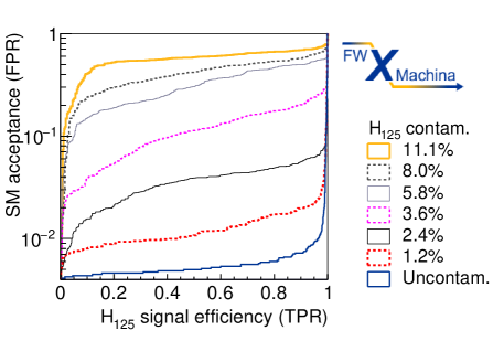
Figure 5: ROC curves showing the signal efficiency vs. SM acceptance for different levels of $H_{125}\rightarrow a_{10}a_{15}\rightarrow e^{+}e^{-}\mu^{+}\mu^{-}$ signal contamination mixed with the SM sample that is used to train the autoencoder. The plot is software-simulated results using bit integers as done in the firmware.

The Supplemental Fig. A.4 shows a possible experimental setup of employing a set of autoencoders with varying levels of simulated signal contamination to compare to the autoencoder trained on a sample of collected data.

4 Discussion

A novel implementation of a decision tree-based autoencoder anomaly detector was presented. The fwXmachina framework is used to implement the algorithm on FPGA with the goal of conducting real-time anomaly detection for physics beyond the Standard Model at real-time trigger systems at high energy physics experiments. The implementation is tested on two problems: detection of exotic Higgs decays to $e^{+}e^{-}\mu^{+}\mu^{-}$ through pseudoscalar intermediates and an LHC physics anomaly detection dataset [73]. In both problems, the ML is trained only on background processes and evaluated on both signal and background. The anomaly detector shows the promise to identify several different realistic exotic signals that may be seen at a trigger system with comparable physics performance to existing neural network-based anomaly detectors. The ultraefficient firmware implementation and ultrafast latency of $25\,\textrm{ns}$ is the time between successive collisions at the LHC.

The anomaly score distributions for the two problems show patterns that may help plan for the different types of BSM physics that may be detected. The two anomaly distributions for $H_{125}$ and $H_{70}\rightarrow aa^{\prime}\rightarrow e^{+}e^{-}\mu^{+}\mu^{-}$ are narrow, reflecting the relatively excellent invariant mass resolution of the input distributions. In contrast, the four anomaly distributions for the LHC physics dataset are relatively broad, since the input variables are the final state momentum vectors $(p_{\textrm{T}},\eta,\phi)$ without narrow distributions. The importance of the narrow distributions on top of a smoothly falling background, such as for $H_{70}$, necessitates a different approach in real-time systems because the trigger selection is generally a one-sided threshold selection. A selection window with a dedicated online trigger system could include training methods using AE methods described in this paper, which define the selection window by rapidly analyzing the data that would otherwise be rejected.

A study of classifier performance with signal contamination shows the promise for the possibility to train on the collected data at the LHC. If the collected data already has BSM processes mixed in that we are trying to discover, then this possibility allows one to train the ML with the data anyway then deploy it on future data to detect the BSM signal [88]. These approaches may also be of interest at the High Luminosity LHC (HL-LHC) [89], which will increase the rate of proton collisions at the cost of higher background levels.

Existing approaches of the real-time trigger path anomaly detector, including the one in this paper, make assumptions about the availability of the preprocessed “objects” such as electrons that are reconstructed from more basic inputs such as calorimetric data. The next step would consider such inputs ranging from $1$k to $100$M channels, depending on the experimental setup, which may require a drastic redesign of existing approaches.

Data availability

Two datasets were used in this paper. The one used in Sec. 3.1 is created by us and is publicly available on Mendeley [90]. The other used in Sec. 3.2 was taken from Ref. [73] and is publicly available.

Code availability

The repository with the files to evaluate the FPGA performance is publicly available at D-Scholarship@Pitt, which is an institutional repository for the research output of the University of Pittsburgh [91]. More specifically, the IP core design for the benchmark scenario is available along with a testbench and associated test vectors.

General information about fwXmachina can be found at http://fwx.pitt.edu.

Author contributions

STR, JS, WCO, and TMH designed the ML training algorithm. QB and PS implemented and tested the firmware design. STR, BTC, and TMH created the simulated dataset and performed the physics analysis. STR led the project execution while TMH managed and coordinated the overall effort. TMH and STR drafted the manuscript with significant inputs from BTC. All authors reviewed the manuscript.

Appendix A Supplemental figures

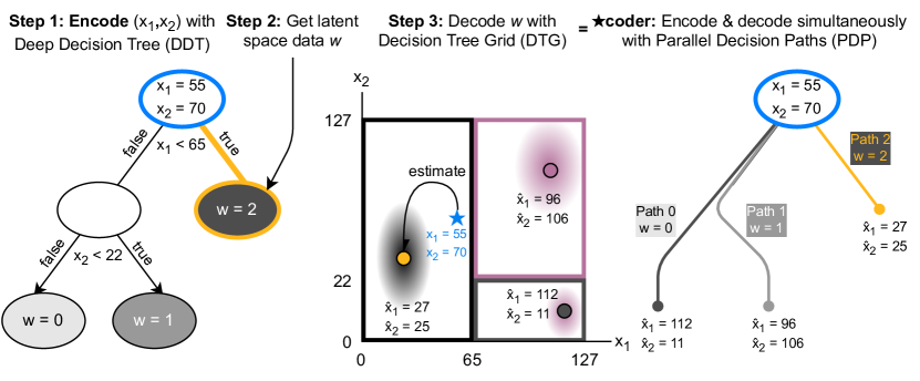
Figure A.1: Illustrative example of $\star$coder as two visual representations of the same decision tree. Deep decision tree (left) rendered as the decision tree grid (center) and implemented by the parallel decision paths (right). Two-depth deep decision tree (DDT) is the encoder (step 1) shown as a conventional binary split diagram; the latent space is the bin number (step 2); the latent space data is decoded using the decision tree grid (DTG) (step 3); and the simultaneous encoding and decoding with $\star$coder (star-coder) architecture (right) represented by parallel decision paths (PDP) of Ref. [71]. The DTG is the visualization as a grid of partitions in $V$-dimensional space. In this example, the input $\mathbf{x}{\,=\,}(55,70)$ yields the output $\hat{\textbf{x}}{\,=\,}(27,25)$ without needing to explicitly produce the latent layer.

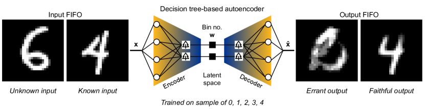
Figure A.2: Demonstration of decision tree-based autoencoder and a demonstration of data transmission / anomaly detection using the mnist dataset, which is a set of images of handwritten numbers converted to $28\times 28$ pixels, or $784$-length input vector $V=784$, with $N=8$ bits per pixel. The ML training is done on $15$k images of handwritten $0$ to $4$, but not $5$ to $9$, on one tree $T=1$ at a maximum depth of $D=20$. The output is a $784$-length vector with $8$ bits per pixel. The data compression-decompression factor, the ratio of input-output bits to the latent space dimensions, $V\cdot N/(T\cdot D)=784\cdot 8/(1\cdot 20)$, is about 300. The figure shows two input-output pairs as examples. The output of $4$ resembles $4$ while the output of $6$ is garbled. The former yields a smaller input-output distance relative to the latter case. The input data shown here are not part of the training sample.

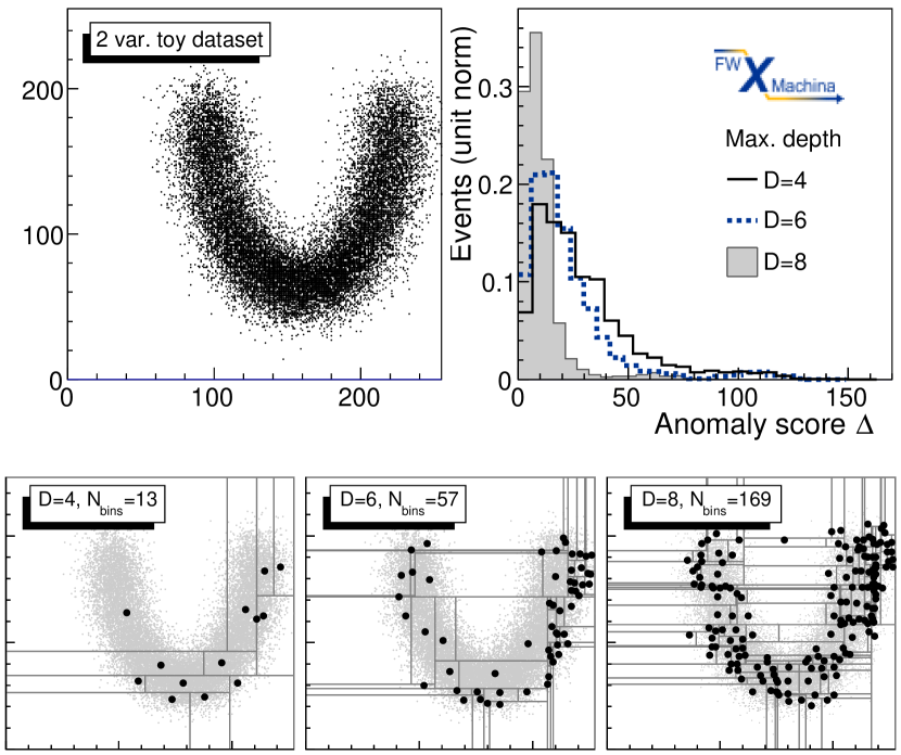
Figure A.3: Toy dataset and ML training with varying maximum depth $D$. The top-left plot shows training sample where each data point is represented by a 2d coordinate. The top-right plot shows input-output distance $\Delta$ for various $D$. The anomaly score distribution shows RMS shrinking with $D$ when evaluated on a sample similar to the training sample. The bottom rows of plots shows the result of the ML training. In each partition, a dot ($\bullet$) indicates the estimate $\hat{\mathbf{x}}$, the location of the median in each dimension of the data in that bin, corresponding to the bin that $\mathbf{x}$ resides in. With the median points one can visualize the refinement of the reconstruction of the original dataset with increasing $D$.

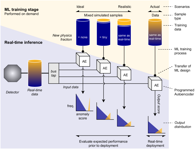
Figure A.4: Illustration of the ML training with varying levels of signal contamination (top) and the real-time inference (bottom). This setup can help prepare the scenario where the autoencoder is trained using the incoming data itself.

References

- [1] L. Evans and P. Bryant, LHC Machine, JINST 3, S08001 (2008).
- [2] ATLAS Collaboration, Observation of a new particle in the search for the Standard Model Higgs boson with the ATLAS detector at the LHC, Phys. Lett. B 716, no. 1, 1 (2012).
- [3] CMS Collaboration, Observation of a new boson at a mass of 125 GeV with the CMS experiment at the LHC, Phys. Lett. B 716, no. 1, 30 (2012).
- [4] ATLAS Collaboration, A detailed map of Higgs boson interactions by the ATLAS experiment ten years after the discovery, Nature 607, 52–59 (2022).
- [5] CMS Collaboration, A portrait of the Higgs boson by the CMS experiment ten years after the discovery, Nature 607, 60–68 (2022).
- [6] N. Arkani-Hamed and S. Dimopoulos, Supersymmetric unification without low energy supersymmetry and signatures for fine-tuning at the LHC, JHEP 06, 073 (2005).
- [7] X. Tata, Natural supersymmetry: status and prospects, Eur. Phys. J. Spec. Top. 229, 3061–3083 (2020).
- [8] O. Buchmueller, C. Doglioni, and LT. Wang, Search for dark matter at colliders, Nature Phys 13, 217–223 (2017).
- [9] J. A. Aguilar-Saavedra, J. H. Collins, and R. K. Mishra, A generic anti-QCD jet tagger, JHEP 11, 163 (2017).
- [10] J. H. Collins, K. Howe, and B. Nachman, Anomaly Detection for Resonant New Physics with Machine Learning, Phys. Rev. Lett. 121, 241803 (2018).
- [11] R. T. D’Agnolo and A. Wulzer, Learning New Physics from a Machine, Phys. Rev. D 99, no. 1, 015014 (2019).
- [12] O. Cerri, T. Q. Nguyen, M. Pierini, M. Spiropulu, and J. R. Vlimant, Variational Autoencoders for New Physics Mining at the Large Hadron Collider, JHEP 05, 036 (2019).
- [13] J. H. Collins, K. Howe, and B. Nachman, Extending the search for new resonances with machine learning, Phys. Rev. D 99, no. 1, 014038 (2019)
- [14] M. Farina, Y. Nakai, and D. Shih, Searching for New Physics with Deep Autoencoders, Phys. Rev. D 101, 075021 (2020).
- [15] T. Heimel, G. Kasieczka, T. Plehn, and J. M. Thompson, QCD or What?, SciPost Phys. 6, no. 3, 030 (2019).
- [16] A. Blance, M. Spannowsky, and P. Waite, Adversarially-trained autoencoders for robust unsupervised new physics searches, JHEP 10, 047 (2019).
- [17] A. De Simone and T. Jacques, Guiding New Physics Searches with Unsupervised Learning, Eur. Phys. J. C 79, no. 4, 289 (2019).
- [18] B. M. Dillon, D. A. Faroughy, and J. F. Kamenik, Uncovering latent jet substructure, Phys. Rev. D 100, no. 5, 056002 (2019).
- [19] J. Hajer, Y. Y. Li, T. Liu, and H. Wang, Novelty Detection Meets Collider Physics, Phys. Rev. D 101, no. 7, 076015 (2020).
- [20] A. Andreassen, B. Nachman, and D. Shih, Simulation Assisted Likelihood-free Anomaly Detection, Phys. Rev. D 101, no. 9, 095004 (2020).
- [21] B. Nachman and D. Shih, Anomaly Detection with Density Estimation, Phys. Rev. D 101, 075042 (2020).
- [22] B. M. Dillon, D. A. Faroughy, J. F. Kamenik, and M. Szewc, Learning the latent structure of collider events, JHEP 10, 206 (2020).
- [23] A. A. Pol, V. Berger, G. Cerminara, C. Germain, and M. Pierini, Anomaly Detection With Conditional Variational Autoencoders, 2020, [2010.05531].
- [24] R. T. D’Agnolo, G. Grosso, M. Pierini, A. Wulzer, and M. Zanetti, Learning multivariate new physics, Eur. Phys. J. C 81, no. 1, 89 (2021)
- [25] A. Mullin, S. Nicholls, H. Pacey, M. Parker, M. White, and S. Williams, Does SUSY have friends? A new approach for LHC event analysis, JHEP 02, 160 (2021).
- [26] M. Crispim Romão, N. F. Castro, and R. Pedro, Finding New Physics without learning about it: Anomaly Detection as a tool for Searches at Colliders, Eur. Phys. J. C 81, no.1, 27 (2021), [erratum: Eur. Phys. J. C 81, no. 11, 1020 (2021)].
- [27] M. van Beekveld, S. Caron, L. Hendriks, P. Jackson, A. Leinweber, S. Otten, R. Patrick, R. Ruiz De Austri, M. Santoni, and M. White, Combining outlier analysis algorithms to identify new physics at the LHC, JHEP 09, 024 (2021).
- [28] G. Kasieczka, B. Nachman, D. Shih, O. Amram, A. Andreassen, K. Benkendorfer, B. Bortolato, G. Brooijmans, F. Canelli, J. H. Collins, et al., The LHC Olympics 2020 a community challenge for anomaly detection in high energy physics, Rept. Prog. Phys. 84, no. 12, 124201 (2021).
- [29] J. A. Aguilar-Saavedra, F. R. Joaquim, and J. F. Seabra, Mass Unspecific Supervised Tagging (MUST) for boosted jets, JHEP 03, 012 (2021), [erratum: JHEP 04, 133 (2021)].
- [30] V. Mikuni and F. Canelli, Unsupervised clustering for collider physics, Phys. Rev. D 103, no. 9, 092007 (2021).
- [31] T. Finke, M. Krämer, A. Morandini, A. Mück, and I. Oleksiyuk, Autoencoders for unsupervised anomaly detection in high energy physics, JHEP 06, 161 (2021).
- [32] K. Benkendorfer, L. L. Pottier, and B. Nachman, Simulation-assisted decorrelation for resonant anomaly detection, Phys. Rev. D 104, no. 3, 035003 (2021).
- [33] J. H. Collins, P. Martín-Ramiro, B. Nachman, and D. Shih, Comparing weak- and unsupervised methods for resonant anomaly detection, Eur. Phys. J. C 81, no. 7, 617 (2021).
- [34] B. M. Dillon, T. Plehn, C. Sauer, and P. Sorrenson, Better Latent Spaces for Better Autoencoders, SciPost Phys. 11, 061 (2021).
- [35] O. Atkinson, A. Bhardwaj, C. Englert, V. S. Ngairangbam, and M. Spannowsky, Anomaly detection with convolutional Graph Neural Networks, JHEP 08, 080 (2021).
- [36] A. Kahn, J. Gonski, I. Ochoa, D. Williams, and G. Brooijmans, Anomalous jet identification via sequence modeling, JINST 16, no.08, P08012 (2021).
- [37] T. Aarrestad, M. van Beekveld, M. Bona, A. Boveia, S. Caron, J. Davies, A. De Simone, C. Doglioni, J. M. Duarte, A. Farbin, et al., The Dark Machines Anomaly Score Challenge: Benchmark Data and Model Independent Event Classification for the Large Hadron Collider, SciPost Phys. 12, no. 1, 043 (2022).
- [38] V. Mikuni, B. Nachman, and D. Shih, Online-compatible Unsupervised Non-resonant Anomaly Detection, Phys. Rev. D 105, no. 5, 055006 (2022).
- [39] P. Jawahar, T. Aarrestad, N. Chernyavskaya, M. Pierini, K. A. Wozniak, J. Ngadiuba, J. Duarte, and S. Tsan, Improving Variational Autoencoders for New Physics Detection at the LHC With Normalizing Flows, Front. Big Data 5, 803685 (2022).
- [40] S. Chekanov and W. Hopkins, Event-Based Anomaly Detection for Searches for New Physics, Universe 8, no.10, 494 (2022).
- [41] A. Hallin, J. Isaacson, G. Kasieczka, C. Krause, B. Nachman, T. Quadfasel, M. Schlaffer, D. Shih, and M. Sommerhalder, Classifying anomalies through outer density estimation, Phys. Rev. D 106, no. 5, 055006 (2022).
- [42] K. Fraser, S. Homiller, R. K. Mishra, B. Ostdiek, and M. D. Schwartz, Challenges for unsupervised anomaly detection in particle physics, JHEP 03, 066 (2022).
- [43] B. Bortolato, A. Smolkovič, B. M. Dillon, and J. F. Kamenik, Bump hunting in latent space, Phys. Rev. D 105, no. 11, 115009 (2022).
- [44] S. Caron, L. Hendriks, and R. Verheyen, Rare and Different: Anomaly Scores from a combination of likelihood and out-of-distribution models to detect new physics at the LHC, SciPost Phys. 12, no.2, 077 (2022).
- [45] S. Volkovich, F. De Vito Halevy, and S. Bressler, A data-directed paradigm for BSM searches: the bump-hunting example, Eur. Phys. J. C 82, no. 3, 265 (2022).
- [46] B. Ostdiek, Deep Set Auto Encoders for Anomaly Detection in Particle Physics, SciPost Phys. 12, no. 1, 045 (2022).
- [47] J. A. Aguilar-Saavedra, Anomaly detection from mass unspecific jet tagging, Eur. Phys. J. C 82, no. 2, 130 (2022).
- [48] R. Tombs and C. G. Lester, A method to challenge symmetries in data with self-supervised learning, JINST 17, no. 08, P08024 (2022).
- [49] R. T. d’Agnolo, G. Grosso, M. Pierini, A. Wulzer, and M. Zanetti, Learning new physics from an imperfect machine, Eur. Phys. J. C 82, no. 3, 275 (2022).
- [50] F. Canelli, A. de Cosa, L. L. Pottier, J. Niedziela, K. Pedro, and M. Pierini, Autoencoders for semivisible jet detection, JHEP 02, 074 (2022).
- [51] L. Bradshaw, S. Chang, and B. Ostdiek, Creating simple, interpretable anomaly detectors for new physics in jet substructure, Phys. Rev. D 106, no. 3, 035014 (2022).
- [52] J. A. Aguilar-Saavedra, Taming modeling uncertainties with mass unspecific supervised tagging, Eur. Phys. J. C 82, no. 3, 270 (2022).
- [53] B. M. Dillon, R. Mastandrea, and B. Nachman, Self-supervised anomaly detection for new physics, Phys. Rev. D 106, no. 5, 056005 (2022).
- [54] M. Birman, B. Nachman, R. Sebbah, G. Sela, O. Turetz, and S. Bressler, Data-directed search for new physics based on symmetries of the SM, Eur. Phys. J. C 82, no. 6, 508 (2022).
- [55] M. Letizia, G. Losapio, M. Rando, G. Grosso, A. Wulzer, M. Pierini, M. Zanetti, and L. Rosasco, Learning new physics efficiently with nonparametric methods, Eur. Phys. J. C 82, no. 10, 879 (2022).
- [56] C. Fanelli, J. Giroux, and Z. Papandreou, Flux+Mutability: a conditional generative approach to one-class classification and anomaly detection, Mach. Learn. Sci. Tech. 3, no. 4, 045012 (2022).
- [57] R. Verheyen, Event Generation and Density Estimation with Surjective Normalizing Flows, SciPost Phys. 13, no. 3, 047 (2022).
- [58] T. Cheng, J. F. Arguin, J. Leissner-Martin, J. Pilette, and T. Golling, Variational autoencoders for anomalous jet tagging, Phys. Rev. D 107, no. 1, 016002 (2023).
- [59] S. Caron, R. R. de Austri, and Z. Zhang, Mixture-of-Theories training: can we find new physics and anomalies better by mixing physical theories?, JHEP 03, 004 (2023).
- [60] T. Dorigo, M. Fumanelli, C. Maccani, M. Mojsovska, G. C. Strong, and B. Scarpa, RanBox: anomaly detection in the copula space, JHEP 01, 008 (2023).
- [61] G. Kasieczka, R. Mastandrea, V. Mikuni, B. Nachman, M. Pettee, and D. Shih, Anomaly detection under coordinate transformations, Phys. Rev. D 107, no. 1, 015009 (2023).
- [62] J. F. Kamenik and M. Szewc, Null hypothesis test for anomaly detection, Phys. Lett. B 840, 137836 (2023).
- [63] K. Krzyżańska and B. Nachman, Simulation-based anomaly detection for multileptons at the LHC, JHEP 01, 061 (2023).
- [64] ATLAS Collaboration, Dijet resonance search with weak supervision using TeV collisions in the ATLAS detector, Phys. Rev. Lett. 125, no. 13, 131801 (2020).
- [65] O. Knapp, O. Cerri, G. Dissertori, T. Q. Nguyen, M. Pierini, and J. R. Vlimant, Adversarially Learned Anomaly Detection on CMS Open Data: re-discovering the top quark, Eur. Phys. J. Plus 136, no. 2, 236 (2021).
- [66] ATLAS Collaboration, Anomaly detection search for new resonances decaying into a Higgs boson and a generic new particle X in hadronic final states using TeV pp collisions with the ATLAS detector, ATLAS-CONF-2022-045, 2022, https://cds.cern.ch/record/2816323.
- [67] ATLAS Collaboration, The ATLAS Experiment at the CERN Large Hadron Collider, JINST 3, S08003 (2008).
- [68] CMS Collaboration, The CMS Experiment at the CERN LHC, JINST 3, S08004 (2008).
- [69] E. Govorkova, E. Puljak, T. Aarrestad, T. James, V. Loncar, M. Pierini, A.A. Pol, N. Ghielmetti, M. Graczyk, S. Summers, et al., Autoencoders on field-programmable gate arrays for real-time, unsupervised new physics detection at 40 MHz at the Large Hadron Collider, Nat. Mach. Intell. 4, 154-161 (2022), [author correction: Nat. Mach. Intell. 4, 414 (2022)].
- [70] T.M. Hong, B.T. Carlson, B.R. Eubanks, S.T. Racz, S.T. Roche, J. Stelzer, and D.C. Stumpp, Nanosecond machine learning event classification with boosted decision trees in FPGA for high energy physics, JINST 16, P08016 (2021).
- [71] B.T. Carlson, Q. Bayer, T.M. Hong, and S.T. Roche, JINST 17 P09039 (2022) Nanosecond machine learning regression with deep boosted decision trees in FPGA for high energy physics, JINST 17, P09039 (2022).
- [72] D. Curtin, R. Essig, S. Gori, P. Jaiswal, A. Katz, T. Liu, Z. Liu, D. McKeen, J. Shelton, M. Strassler, et al., Exotic decays of the 125 GeV Higgs boson, Phys. Rev. D 90, no. 7, 075004 (2014).
- [73] E. Govorkova, E. Puljak, T. Aarrestad, M. Pierini, K. A. Woźniak and J. Ngadiuba, LHC physics dataset for unsupervised New Physics detection at 40 MHz, Sci. Data 9, no. 118, (2022).
- [74] J. Feng and Z. Zhou, AutoEncoder by Forest, AAAI Conference on Artificial Intelligence, 2017, [1709.09018].
- [75] O. İrsoy and E. Alpaydın, Unsupervised feature extraction with autoencoder trees, Neurocomputing 258, 63-73 (2017).
- [76] F. T. Liu, K. M. Ting, and Z. Zhou, Isolation forest, 8 IEEE Int’l Conf. on Data Mining, 413-422 (2008).
- [77] Mohd Adli Md Ali, N. Badrud’din, H. Abdullah, and F. Kemi, Alternate methods for anomaly detection in high-energy physics via semi-supervised learning, Int’l. J. Mod. Phys. A 35, no. 23, 2050131 (2020).
- [78] Y.-C. Guo, L. Jiang, and J.-C. Yang, Detecting anomalous quartic gauge couplings using the isolation forest machine learning algorithm, Phys. Rev. D 104 (3), 035021 (2021).
- [79] J. C. Yang, Y. C. Guo and L. H. Cai, Using a nested anomaly detection machine learning algorithm to study the neutral triple gauge couplings at an collider, Nucl. Phys. B 977, 115735 (2022).
- [80] L. Deng, The MNIST Database of Handwritten Digit Images for Machine Learning Research, IEEE Sig. Proc. Mag. 29, no. 6, 141-142 (2012).
- [81] G. Di Guglielmo, F. Fahim, C. Herwig, M. Blanco Valentin, J. Duarte, C. Gingu, P. Harris, J. Hirschauer, M. Kwok, V. Loncar, et al., A Reconfigurable Neural Network ASIC for Detector Front-End Data Compression at the HL-LHC, IEEE Trans. Nucl. Sci. 68, no. 8, 2179-2186 (2021).
- [82] J. Alwall et al., The automated computation of tree-level and next-to-leading order differential cross sections, and their matching to parton shower simulations, JHEP 07, 079 (2014).
- [83] T. Sjöstrand et al., An introduction to PYTHIA 8.2, Comput. Phys. Commun. 191, 159-177 (2015).
- [84] S. Ovyn, X. Rouby, and V. Lemaitre, DELPHES, a framework for fast simulation of a generic collider experiment, 2009, [hep-ph/0903.2225].
- [85] DELPHES 3 Collaboration, DELPHES 3, A modular framework for fast simulation of a generic collider experiment, JHEP 02, 057 (2014).
- [86] G. Soyez, Pileup mitigation at the LHC: A theorist’s view Phys. Rept. 803, 1-158 (2019).
- [87] M. Selvaggi et al., The delphes_card_CMS_PileUp.tcl file in Delphes (3.5.1pre07) Zenodo code repository, 2023, https://doi.org/10.5281/zenodo.7733551, accessed March 29, 2023.
- [88] ATLAS and CMS Collaborations, Snowmass White Paper Contribution: Physics with the Phase-2 ATLAS and CMS Detectors ATLAS PUB Note 2022-018 and CMS PAS Note FTR-2022-001, 2022, http://cds.cern.ch/record/2800319.
- [89] ATLAS Collaboration, Technical Design Report for the Phase-II Upgrade of the ATLAS TDAQ System, CERN-LHCC-2017-020, 2017, http://cds.cern.ch/record/2285584.
- [90] S.T. Roche, B.T. Carlson, and T.M. Hong, fwXmachina example: Anomaly detection, Mendeley Data, 2023, http://dx.doi.org/10.17632/y698s5kscs.1.
- [91] T.M. Hong and P. Serhiayenka, Xilinx inputs for nanosecond anomaly detection with decision trees, D-Scholarship@Pitt #44431, 2023, https://d-scholarship.pitt.edu/44431.