Multi-Robot Relative Pose Estimation and IMU Preintegration Using Passive UWB Transceivers

Abstract

Ultra-wideband (UWB) systems are becoming increasingly popular as a means of inter-robot ranging and communication. A major constraint associated with UWB is that only one pair of UWB transceivers can range at a time to avoid interference, hence hindering the scalability of UWB-based localization. In this paper, a ranging protocol is proposed that allows all robots to passively listen on neighbouring communicating robots without any hierarchical restrictions on the role of the robots. This is utilized to allow each robot to obtain more range measurements and to broadcast preintegrated inertial measurement unit (IMU) measurements for relative extended pose state estimation directly on $SE_{2}(3)$. Consequently, a simultaneous clock-synchronization and relative-pose estimator (CSRPE) is formulated using an on-manifold extended Kalman filter (EKF) and is evaluated in simulation using Monte-Carlo runs for up to 7 robots. The ranging protocol is implemented in C on custom-made UWB boards fitted to 3 quadcopters, and the proposed filter is evaluated over multiple experimental trials, yielding up to 56% improvement in localization accuracy.

I Introduction

Multi-robot teams’ prevalence is a direct consequence of two factors, recent advancements in available technology and demand for automating complex tasks. The former has recently been accelerated through the adoption of ultra-wideband (UWB) radio-frequency signals as a means of ranging and communication between robots, where ranging means obtaining distance measurements. UWB is a relatively inexpensive, low-power, lightweight, and compact technology, which allows for high-rate ranging and data transfer. An example of UWB boards fitted to a quadcopter is shown in Figure 1. Robotic teams equipped with UWB and other sensors, such as cameras and/or inertial measurement units (IMUs), have been considered for relative pose estimation, which is a prerequisite for applications such as collision avoidance and collaborative mapping and infrastructure inspection.

(a) Subfigure 1 list of figures text

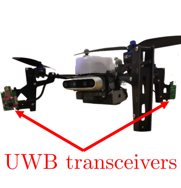
(b) Subfigure 1 list of figures text

Figure 1: The experimental set-up.

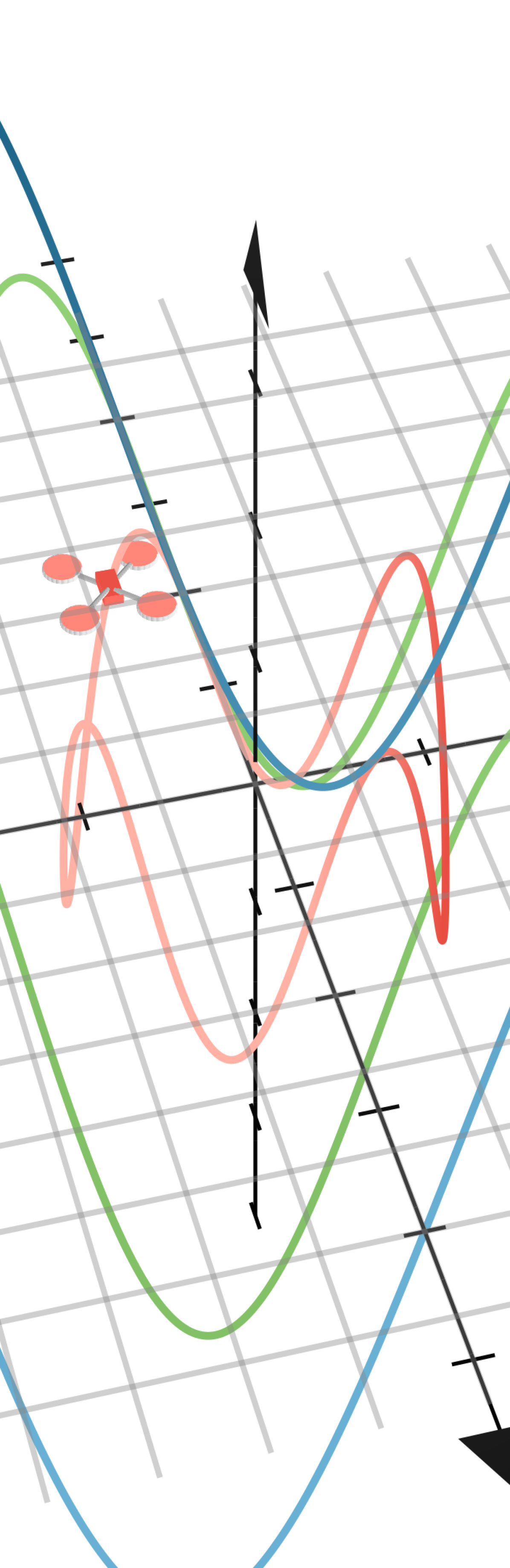
Figure 2: The trajectories followed by three simulated quadcopters.

Nonetheless, using UWB for relative pose estimation in multi-robot teams introduces a distinct set of problems. Firstly, UWB ranging and communication is not robust to interference, thus imposing the constraint that only one pair of transceivers can communicate at a time. This is typically addressed using time-division multiple-access (TDMA) media-access control (MAC) protocols alongside a round-robin approach to determine which pair communicates at each time. However, the larger the team of robots, the longer the time gaps in between a robot ranging with another. Another complication with UWB ranging is the reliance on time-of-flight (ToF) measurements, which necessitates the presence of a clock at each UWB transceiver. However, in practice these clocks run at different rates, and therefore require some synchronization mechanism. The importance of synchronization can be highlighted by the fact that 1 ns in synchronization error translates to $c\text{ [m/s] }\times 10^{-9}\text{ [s] }\approx 30\text{ [cm] }$ in localization error, where $c$ is the speed of light.

Another practical issue associated with multi-robot systems is communication constraints, which limit the amount of information that can be transmitted between robots. In filtering applications where there are for example 3 quadcopters moving randomly in 3-dimensional space as shown in Figure 2, IMU measurements must be broadcasted if robots are to estimate their neighbours’ relative states directly from the raw measurements. Nonetheless, IMU measurements are typically recorded at a very high frequency, and the constraint that only one pair can be communicating at a time means that communication links between robots do not always exist. Therefore, a more efficient way of sharing odometry information is required.

To achieve a practical relative pose estimation solution that is implementable on a robotic team, this paper addresses the aforementioned constraints. The contributions of this work are summarized as follows.

1. A ranging protocol is introduced that extends classical ranging protocols by allowing neighbouring robots to passively listen to the measurements and timestamp receptions, with no assumptions or imposed constraints on the robots’ hierarchy. The concept of passive listening is then utilized to provide a $(1+3n)$-fold increase in the number of measurements recorded when there are a total of $n+1$ robots each equipped with two UWB transceivers. The concept of passive listening is additionally utilized for more efficient information sharing and implementing simple MAC protocols.

2. Representing the extended pose state as an element of $SE_{2}(3)$, an on-manifold tightly-coupled simultaneous clock-synchronization and relative-pose estimator (CSRPE) is then proposed, which allows incoporating passive listening measurements in an extended Kalman filter (EKF) to improve the relative pose estimation. This provides a means for many different robots to estimate the relative poses of their neighbours relative to themselves at a high frequency.

3. Rather than sharing high-frequency IMU readings with neighbours, the concept of preintegration [1] is developed for relative pose states on $SE_{2}(3)$, and is used as a means of efficient IMU data logging and communication between robots. This is additionally incorporated in the CSRPE, where the theory behind filtering with delayed inputs is developed as the preintegrated IMU measurements arrive asynchronously from neighbouring robots.

4. The proposed algorithm is evaluated in simulation using Monte-Carlo trials and in experiments using 4 trials with 3 quadcopters equipped with two UWB transceivers each. It is shown that localization accuracy improves up to 56% for one of the experimental trials when compared to the case of no passive listening.

The remainder of the paper is organized as follows. Related work is presented in Section II, and Lie group and UWB preliminaries are discussed in Section III. The problem is formulated in Section IV, then the proposed ranging protocol is discussed in Section V. The relative-pose process model and preintegration on $SE_{2}(3)$ are discussed in Sections VI and VII, respectively. Simulation and experimental results are discussed in Sections VIII and IX, respectively, before the paper is concluded in Section X.

II Related Work

Figure 3: The distribution of the posterior position of the green robot given a position prior and a single range measurement with the red robot.

The majority of UWB-based localization relies on a set of pre-localized and synchronized static transceivers, or anchors, to localize a mobile transceiver [2, 3, 4]. This typically relies on the anchors ranging with the mobile transceiver using standard ranging protocols such as two-way ranging (TWR) or time-difference-of-arrival (TDoA) [5, 6], [7, Chapter 7.1.4]. More complicated ranging protocols have been proposed in [8, 9, 10] to allow multiple anchors to passively listen-in on messages with the mobile transceiver to localize it.

Calibrating the clocks and location of anchors is challenging, and [11, 12] propose an approach where anchors actively range with one another to synchronize and localize themselves. Meanwhile, the mobile transceiver passively listens to these signals to localize itself using the anchors’ estimated clock states and positions. The work in [13, 14] extends this by applying a Kalman filter (KF) to the synchronization and localization problem. In [15], a localization cost function is proposed that is invariant to the anchors’ synchronization error. Meanwhile, in [16], the synchronization approach is accurate to within a few microseconds, whereas nanosecond-level accuracy is desired for localization with cm accuracy.

Overcoming the need for a fixed infrastructure of anchors, UWB has been used more recently for teams of robots [17, 18, 19]. In [20], it is assumed that neighbouring robots know their poses and clock states, thus essentially behaving as mobile anchors, allowing a mobile transceiver to localize itself. The use of robots with multiple transceivers is proposed in [21, 22], and in [23] a robot equipped with 4 transceivers localizes a mobile transceiver relative to itself by having one of the 4 transceivers actively range with the target and the other 3 passively listening.

In [24, 25], a passive-listening-based ranging protocol is proposed where the network is divided into “parent robots” that actively range with one another and “child robots” that passively listen-in on these measurements. This hierarchical constraint has the limitation that parent robots cannot localize child robots and do not benefit from passive listening measurements themselves when they are not involved in a ranging transaction. Additionally, it is suggested that the child robots use the estimated position and clock states of the parent states, which in filtering applications would lead to untracked cross-correlations that would result in poor performance [26].

Furthermore, in filtering applications, the problem of communicating IMU measurements to neighbours remains unaddressed. In [27, 28], scattering theory is used to send pre-computed matrices between two robots rather than individual IMU measurements, in a manner similar to the concept of preintegration [29, 1]. However, extending this to more than two robots is challenging, particularly for preintegrated poses directly on $SE_{2}(3)$ [30, 31]. Relative pose estimation using range measurements is inherently a nonlinear problem, which is commonly addressed using particle filtering [32, 33] to handle non-ellipsoid-shaped distributions in Cartesian coordinates, see Figure 3. This nonlinearity motivates the use of an on-manifold EKF, which can represent such distributions using exponential coordinates [34].

III Preliminaries

III-A Notation

Throughout this paper, a bold upper-case letter (e.g., $\mbf{X}$) denotes a matrix, a bold lower-case letter (e.g., $\mbf{x}$) denotes a column matrix, and a right arrow under the letter (e.g., $\underrightarrow{x}$) denotes a physical vector. In a 3-dimensional space, a vector $\underrightarrow{x}$ resolved in a reference frame $i$ is denoted as $\mbf{x}_{i}\in\mathbb{R}^{3}$, while the derivative of a vector $\underrightarrow{x}$ with respect to frame $i$ is denoted ${}^{i}\underrightarrow{\dot{x}}$.

The vector from point $w$ to point $z$ is denoted $\underrightarrow{r}^{zw}$. The relative velocity and acceleration between points $z$ and $w$ with respect to frame $i$ is denoted

$$\underrightarrow{v}^{zw/i}\triangleq\hskip 4.0pt^{i}\underrightarrow{\dot{r}}^{zw},\qquad\underrightarrow{a}^{zw/i}\triangleq\hskip 4.0pt^{i}\underrightarrow{\dot{v}}^{zw/i}.$$

The rotation from a reference frame $j$ to a reference frame $i$ is parametrized using a rotation matrix $\mbf{C}_{ij}\in SO(3)$. Therefore, the relationship between $\mbf{r}_{i}^{zw}$ and $\mbf{r}_{j}^{zw}$ is given by $\mbf{r}_{i}^{zw}\equiv\mbf{C}_{ij}\mbf{r}_{j}^{zw}$.

Throughout this paper, $\mbf{1}$ and $\mbf{0}$ denote identity and zero matrices of appropriate dimension. When ambiguous, a subscript will indicate the dimension of these matrices.

III-B Matrix Lie Groups

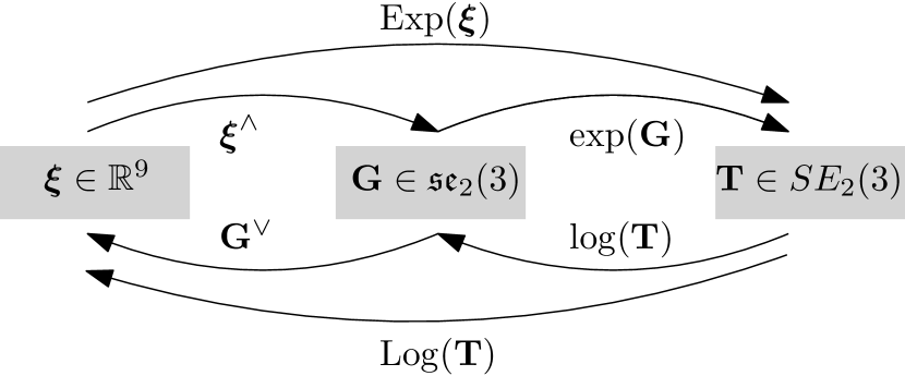
Figure 4: A summary of the operators between elements of the different spaces associated with $SE_{2}(3)$.

The pose of one rigid body relative to another is defined using the relative attitude and position $(\mbf{C},\mbf{r})$, where all subscripts and superscripts are dropped in this section for conciseness. Meanwhile, the extended pose of one rigid body relative to another is defined using the relative attitude, velocity, and position $(\mbf{C},\mbf{v},\mbf{r})$. The extended pose can be represented using an extended pose transformation matrix [30]

$$\mbf{T}=\left[\begin{array}[]{ccc}\mbf{C}&\mbf{v}&\mbf{r}\\ &1&\\ &&1\end{array}\right]\in SE_{2}(3),$$

where empty spaces represent $\mbf{0}$ entries. The corresponding matrix Lie algebra is denoted as $\mathfrak{se}_{2}(3)\subset\mathbb{R}^{5\times 5}$, and elements of this Lie algebra can also be represented as elements of $\mathbb{R}^{9}$. The operators between elements of the different spaces are summarized in Figure 4, and their expression is found in [30, 31],[35, Chapter 9]. Two other useful operators on $SE_{2}(3)$ are the Adjoint operator $\operatorname{Ad}:SE_{2}(3)\rightarrow\mathbb{R}^{9\times 9}$ defined by

$$\operatorname{Exp}(\operatorname{Ad}(\mbf{T})\bm{\xi})\triangleq\mbf{T}\operatorname{Exp}(\bm{\xi})\mbf{T}^{-1},$$

and the odot operator $(\cdot)^{\odot}:\mathbb{R}^{5}\rightarrow\mathbb{R}^{5\times 9}$ defined such that

$$\mbf{p}^{\odot}\bm{\xi}\triangleq\bm{\xi}^{\wedge}\mbf{p}$$ (1)

for any vector $\mbf{p}\in\mathbb{R}^{5}$.

Matrix Lie group elements can be perturbed from the left

$$\mbf{T}=\operatorname{Exp}(\delta\bm{\xi})\bar{\mbf{T}}$$

or the right

$$\mbf{T}=\bar{\mbf{T}}\operatorname{Exp}(\delta\bm{\xi}),$$

where the overbar denotes a nominal value. Additionally, the first-order approximation

$$\operatorname{Exp}(\delta{\bm{\xi}})\approx\mbf{1}+\delta{\bm{\xi}}^{\wedge}$$ (2)

will often be used when linearizing nonlinear models.

III-C UWB Ranging and Clocks

UWB ranging between two transceivers relies on ToF measurements, which are deduced from timestamps recorded by a clock on each transceiver. However, these clocks are unsynchronized. Denoting $t_{i}(t)$ as the time $t$ resolved in Transceiver $i$’s clock gives

$$t_{i}(t)=t+\tau_{i}(t),$$ (3)

where $\tau_{i}(t)$ defines the (time-varying) offset of clock $i$.

To obtain a range measurement, the two transceivers transmit and timestamp a sequence of messages among themselves as shown between Robot 1 and Robot 2 in Figure 6. A time instance corresponding to the $i^{\text{th}}$ message is denoted as $\mathtt{T}^{i}$ for the transmission time and $\mathtt{R}^{i}$ for the reception time, while a subscript $j$ denotes the time instance as timestamped by Transceiver $j$. For example, $\mathtt{T}^{1}_{f_{0}}$ is the timestamp corresponding to the first message transmission as recorded by Transceiver $f_{0}$. The protocol example shown between Robot 1 and Robot 2 in Figure 6 is a modified version of the standard double-sided two-way ranging (DS-TWR [36]) protocol as presented in [6], where the message shown in red represents an “information message” used to broadcast the timestamps recorded by Robot 1.

IV Problem Formulation

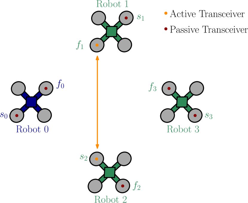
Figure 5: An example of a ranging transaction, where Transceivers $f_{1}$ and $s_{2}$ are actively ranging with one another and all other tags are passively listening.

Consider a scenario with $n+1$ robots, as shown in Figure 5 for $n=3$. Throughout this paper, the perspective of one robot is considered, denoted without loss of generality Robot 0, as any of the $n+1$ robots can be considered Robot 0. Neighbouring robots are then referred to as Robot $i$, $i\in\{1,\ldots,n\}$. This paper employs a “robocentric” viewpoint of the relative-pose state estimation problem, where all states are estimated relative to Robot 0 and are resolved in the body frame of that robot. The robots are assumed to be rigid bodies, so any vector can be resolved in one of the following $n+2$ reference frames:

• an (absolute) inertial frame denoted with a subscript $a$,

• Robot 0’s body frame denoted with a subscript 0, or

• neighbouring Robot $i$’s body frame denoted with a subscript $i$.

Each robot is equipped with an IMU at its center, consisting of a 3-axis gyroscope and accelerometer. Given the use of accelerometers, the relative pose estimation problem involves estimating the extended pose of each neighbouring robot relative to Robot 0 in Robot 0’s body frame. The extended pose of Robot $i$ is then defined as

$$\mbf{T}_{0i}=\left[\begin{array}[]{ccc}\mbf{C}_{0i}&\mbf{v}_{0}^{i0/a}&\mbf{r}_{0}^{i0}\\ &1&\\ &&1\end{array}\right]\in SE_{2}(3),\quad i\in\{1,\ldots,n\},$$

where time dependence is omitted from the notation for conciseness. The dependence on the absolute frame $a$ is also omitted from the notation $\mbf{T}_{0i}$, with the convention that all extended relative pose matrices in the paper are of this form, where the vector corresponding to the second component in the first row is the derivative with respect to the absolute frame of the vector corresponding to the third component, irrespective of the fact that these vectors are resolved in frame $0$.

Each robot is also equipped with 2 UWB transceivers for relative pose observability [21]. The first and second transceivers on Robot $j$ are denoted $f_{j}$ and $s_{j}$, respectively, for $j\in\{0,\ldots,n\}$. It is assumed that the vector coordinates $\mbf{r}_{j}^{f_{j}j}$ and $\mbf{r}_{j}^{s_{j}j}$ between the transceivers and the IMU on Robot $j$ are known, since they can be measured by hand or more accurately using a motion capture system.

Denote the set of all transceivers as $\mathcal{C}=\{f_{0},\ldots,f_{n},s_{0},\ldots,s_{n}\}$. Consider the state of the clock on Transceiver $i\in\mathcal{C}$ relative to real time. The evolution of the offset $\tau_{i}(t)$ of clock $i$ is modelled using a third-order model in [12]. However,[14] shows that a second-order model of the form

$$\underbrace{\left[\begin{array}[]{c}\dot{\tau}_{i}\\ \dot{\gamma}_{i}\end{array}\right]}_{\dot{\mbf{c}}_{i}}=\underbrace{\left[\begin{array}[]{cc}0&1\\ 0&0\end{array}\right]}_{\mbf{A}}\underbrace{\left[\begin{array}[]{c}\tau_{i}\\ \gamma_{c}\end{array}\right]}_{\mbf{c}_{i}}+\mbf{w}_{i}$$ (4)

is sufficient for localization purposes, where $\gamma_{i}(t)$ is called the clock skew, $\mbf{w}_{i}$ is a continuous-time zero-mean white Gaussian process noise with $\mathbb{E}[\mbf{w}_{i}(t_{1})\mbf{w}_{i}(t_{2})]=\bm{\mathcal{Q}}\delta(t_{1}-t_{2})$,

$$\bm{\mathcal{Q}}=\left[\begin{array}[]{cc}\mathcal{Q}^{\tau}&\\ &\mathcal{Q}^{\gamma}\end{array}\right],$$

$\delta(\cdot)$ is the Dirac’s delta function, and $\mathcal{Q}^{\tau}$ and $\mathcal{Q}^{\gamma}$ are the clock offset and skew process-noise power spectral densities, respectively.

A robocentric viewpoint is also maintained for the clock states, where offsets and skews of all clocks are estimated relative to the clock of Transceiver $f_{0}$ on Robot 0. The clock state of Transceiver $s_{0}$ is then

$$\mbf{c}_{s_{0}f_{0}}=\left[\begin{array}[]{c}\tau_{s_{0}f_{0}}\\ \gamma_{s_{0}f_{0}}\end{array}\right]{\color[rgb]{0,0,0}\triangleq\left[\begin{array}[]{c}\tau_{s_{0}}-\tau_{f_{0}}\\ \gamma_{s_{0}}-\gamma_{f_{0}}\end{array}\right]}\in\mathbb{R}^{2},$$

while the clock state of neighbouring Robot $i$ is given by

$${\color[rgb]{0,0,0}\bm{\mathcal{X}}_{i0}^{\text{c}}\triangleq}\left(\mbf{c}_{f_{i}f_{0}},\mbf{c}_{s_{i}f_{0}}\right)\in\mathbb{R}^{2}\times\mathbb{R}^{2},\quad i\in\{1,\ldots,n\},$$

where, as before, time dependence is omitted from the notation for conciseness. The full relative state estimate of Robot $i$ is then given by

$$\bm{\mathcal{X}}_{i0}\triangleq(\mbf{T}_{0i},{\color[rgb]{0,0,0}\bm{\mathcal{X}}_{i0}^{\text{c}}})\in SE_{2}(3)\times\mathbb{R}^{2}\times\mathbb{R}^{2},$$

and the full state estimated by Robot 0 is

$$\bm{\mathcal{X}}\triangleq(\mbf{c}_{s_{0}f_{0}},\bm{\mathcal{X}}_{10},\ldots,\bm{\mathcal{X}}_{n0})\in\mathbb{R}^{2}\times\left(SE_{2}(3)\times\mathbb{R}^{2}\times\mathbb{R}^{2}\right)^{n}.$$

Communication constraints limit Robot 0’s ability to estimate the state $\bm{\mathcal{X}}$, since to prevent interference only one pair of transceivers can communicate at a time. As the number of transceivers increases, this can result in poor scalability due to longer wait times between successive ranging measurements by a given pair. Additionally, the rate at which transceivers communicate is typically lower than the rate at which IMU measurements are recorded at neighbouring robots, thus Robot 0 cannot collect the IMU measurements from all its neighbours without significant and impractical communication overhead. Therefore, part of the problem is to design a scalable and practical ranging protocol that accomodates these communication constraints.

This paper presents an on-manifold extended Kalman filter (EKF) for estimating the state $\bm{\mathcal{X}}$ using a novel ranging protocol that allows all robots to listen-in on neighbours while awaiting their turn to communicate. It is known from [21, 37] that the relative pose states are observable from IMU and range measurements. Meanwhile, to ensure observability of the clock states, clock-offset measurements are sufficient [14].

It is worth mentioning that the size of the state $\bm{\mathcal{X}}$ increases with $n$; therefore, the number of robots that can be included in Robot 0’s EKF is limited by Robot 0’s computational capabilities. This paper addresses the scenario where $n$ is limited to a few robots. However, a potential extension of this work for larger teams would be to have each robot only estimate the relative states of $m<n$ neighbouring robots.

V Ranging Protocol

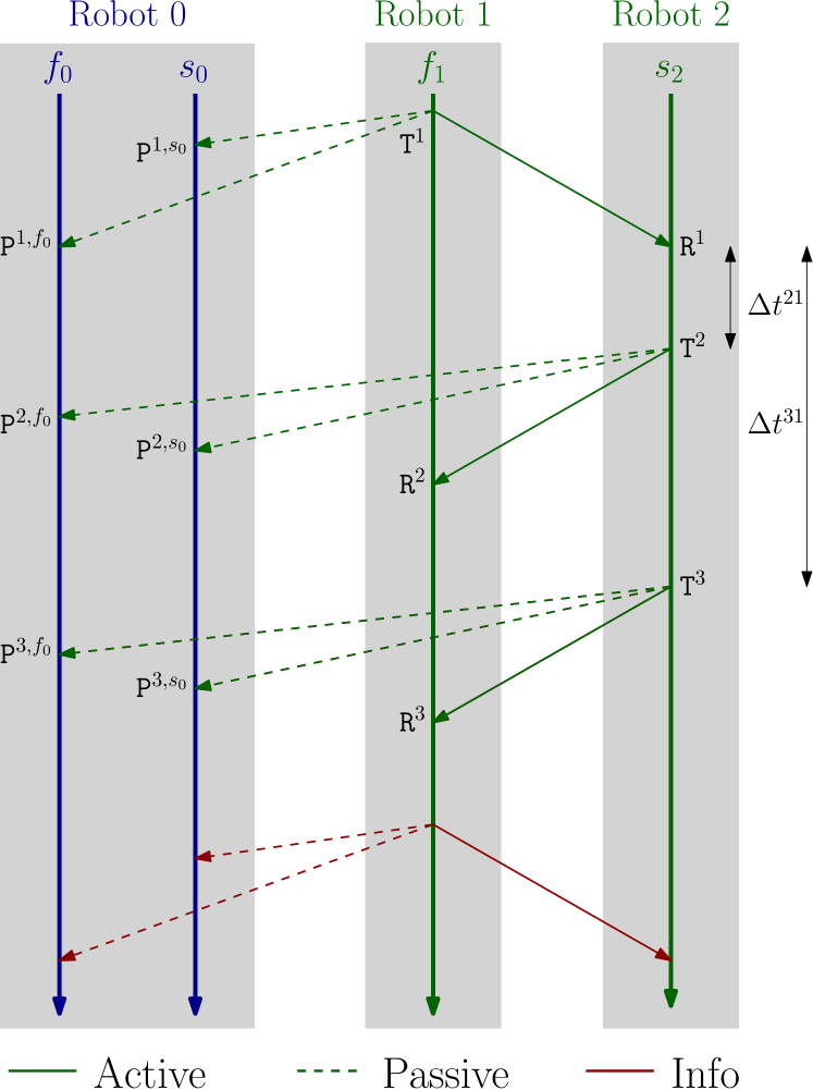
Figure 6: Proposed ranging protocol when Transceiver $f_{1}$ is initiating a DS-TWR ranging transaction with Transceiver $s_{2}$. This paper proposes that all other transceivers listen in on these messages. Shown here are Transceivers $f_{0}$ and $s_{0}$ on Robot 0 passively listening, where the time instance corresponding to the $i^{\text{th}}$ passive reception at Transceiver $j$ is denoted $\mathtt{P}^{i,j}$.

V-A Overview

To address the communication constraints, a ranging protocol is proposed that involves performing DS-TWR between all pairs of transceivers not on the same robot in sequence while leveraging passive listening measurements at all other transceivers that are not actively ranging. This is shown in Figure 6 for an example where Transceiver $f_{1}$ is initiating a TWR transaction with transceiver $s_{2}$, and Transceivers $f_{0}$ and $s_{0}$ are passively listening. In the proposed ranging protocol, any of the $2(n+1)$ transceivers can initiate a TWR transaction with any of the $2n$ transceivers not on the same robot. In this section, the passive listening measurements are utilized in the relative-pose state estimator as a source of ranging information between the different robots. This is possible due to the tightly-coupled nature of the proposed estimator, which performs both clock synchronization and relative pose estimation, meaning that clock-offset-corrupted passive listening measurements can still be used to correct relative pose states, as cross-correlation information is available between clock states and relative pose states at all times.

There are multiple advantages to passive listening in multi-robot pose estimation applications, three of which are highlighted here.

1. A $(1+3n)$-fold increase in the total number of distinct measurements when considering a centralized approach where passive listening measurements from all robots are available, and a $(\frac{1}{2}+2n)$-fold increase in the number of distinct measurements when considering the perspective of an individual robot that does not have access to passive listening measurements at other robots. For example, for 5 neighbouring robots, this results in a 16-fold and an 11.5-fold increase in the number of measurements, respectively. The former is purely due to passive listening measurements, while the latter is due to passive listening measurements as well as the ability to obtain direct time-of-flight (ToF) measurements between two neighbouring robots. The proof of this claim is given in Appendix A.

2. The ability to broadcast information such as IMU measurements or estimated maps at a higher rate as any robot can obtain information communicated between two neighbouring robots. This allows the use of multi-robot preintegration in Section VII.

3. The ability to implement simple MAC protocols to avoid interference. Given that each robot knows which robots are currently ranging, a user-defined sequence of ranging pairs can be made known to all robots. Each robot can then keep track of which pair in the sequence is currently ranging, and initiate a TWR transaction to a specified transceiver when it is its turn to do so. This MAC protocol is named here the common-list protocol.

When implementing the ranging protocol, a choice has to be made on the receiving robot’s side (in this case, Robot 2) for the delays $\Delta t^{21}\triangleq\mathtt{T}^{2}-\mathtt{R}^{1}$ and $\Delta t^{31}\triangleq\mathtt{T}^{3}-\mathtt{R}^{1}$. These user-defined parameters affect the frequency and noise of the measurements, and can be chosen based on [38]. Note that $\Delta t^{32}\triangleq\Delta t^{31}-\Delta t^{21}$. Additionally, it will be assumed throughout this paper that the distances between transceivers and the clock skews remain constant during one ranging transaction. These are good approximations for most robotic applications with typical clock rate variations [7, Chapter 7.1.4], [38].

The remainder of this section analyzes how the proposed ranging protocol can be used in a CSRPE. The particular scenario under study is the one shown in Figures 5 and 6, where transceivers on two neighbouring robots are the ones actively ranging. This is the most general case, and scenarios where one of the transceivers on Robot 0 is actively ranging involve similar but simpler derivations. Note that in Figure 6, all timestamps are available at Robot 0 at the end of the transaction shown, because the timestamps recorded at Robot 1 are communicated in the final information message shown in red and the timestamps recorded at Robot 2 are communicated in the last message transmitted by Robot 2.

V-B Modelling Timestamp Measurements

The time instances shown in Figure 6 are only available to the robots as noisy timestamps and in the clocks of the transceivers rather than in the global common time. Therefore, the timestamp measurements are affected by clock offsets, clock skews, and white noise. Modelling these effects, the timestamps available at Robot 1 (hereinafter, the initiating robot) are of the form

$$\tilde{\mathtt{T}}_{f_{1}}^{1} =\mathtt{T}^{1}+\tau_{f_{1}}(\mathtt{T}^{1})+\eta_{f_{1}}^{1},$$ (5)

$$\tilde{\mathtt{R}}_{f_{1}}^{2} =\mathtt{T}^{1}+\frac{2}{c}d^{s_{2}f_{1}}+\Delta t^{21}+\tau_{f_{1}}(\mathtt{R}^{2})+\eta_{f_{1}}^{2},$$ (6)

$$\tilde{\mathtt{R}}_{f_{1}}^{3} =\mathtt{T}^{1}+\frac{2}{c}d^{s_{2}f_{1}}+\Delta t^{31}+\tau_{f_{1}}(\mathtt{R}^{3})+\eta_{f_{1}}^{3},$$ (7)

where $\tilde{(\cdot)}$ here denotes a measured value, $d^{s_{2}f_{1}}$ is the distance between Transceivers $s_{2}$ and $f_{1}$, and $\eta_{i}^{\ell}$ is the random noise on the $\ell^{\text{th}}$ measurement of Transceiver $i$. All the random noise variables on timestamps are assumed to be independent, zero-mean and with the same variance $\sigma^{2}$.

Similarly, the measurements available at Robot 2 (hereinafter, the target robot) are of the form

$$\tilde{\mathtt{R}}_{s_{2}}^{1} =\mathtt{T}^{1}+\frac{1}{c}d^{s_{2}f_{1}}+\tau_{s_{2}}(\mathtt{R}^{1})+\eta_{s_{2}}^{1},$$ (8)

$$\tilde{\mathtt{T}}_{s_{2}}^{2} =\mathtt{T}^{1}+\frac{1}{c}d^{s_{2}f_{1}}+\Delta t^{21}+\tau_{s_{2}}(\mathtt{T}^{2})+\eta_{s_{2}}^{2},$$ (9)

$$\tilde{\mathtt{T}}_{s_{2}}^{3} =\mathtt{T}^{1}+\frac{1}{c}d^{s_{2}f_{1}}+\Delta t^{31}+\tau_{s_{2}}(\mathtt{T}^{3})+\eta_{s_{2}}^{3}.$$ (10)

The timestamp measurements (5)-(10) correspond to the standard DS-TWR protocol, from which ToF pseudomeasurements can be generated. Nonetheless, additional measurements are available at Robot 0 (hereinafter, the passive robot) since its transceivers $f_{0}$ and $s_{0}$ also receive the messages exchanged between the two actively ranging robots. This yields the following additional timestamp measurements at Robot 0,

$$\tilde{\mathtt{P}}_{i}^{1,i} =\mathtt{T}^{1}+\frac{1}{c}d^{f_{1}i}+\tau_{i}(\mathtt{P}^{1,i})+\eta_{i}^{1},$$ (11)

$$\tilde{\mathtt{P}}_{i}^{2,i} =\mathtt{T}^{1}+\frac{1}{c}d^{s_{2}f_{1}}+\frac{1}{c}d^{f_{1}i}+\Delta t^{21}+\tau_{i}(\mathtt{P}^{2,i})+\eta_{i}^{2},$$ (12)

$$\tilde{\mathtt{P}}_{i}^{3,i} =\mathtt{T}^{1}+\frac{1}{c}d^{s_{2}f_{1}}+\frac{1}{c}d^{f_{1}i}+\Delta t^{31}+\tau_{i}(\mathtt{P}^{3,i})+\eta_{i}^{3},$$ (13)

where $i\in\{f_{0},s_{0}\}$. Similarly, each neighbouring robot not involved in the ranging transaction records its own passive listening measurements at its two transceivers. However, these are not shared with other robots as this would require each robot to take its turn transmitting a message.

In the case where Robot 0 is not involved in the ranging transaction and just listens in passively, there are 12 available timestamp measurements at Robot 0, 6 sent by neighbouring robots, and 3 passive-listening timestamps per transceiver on Robot 0. However, when one of the transceivers $f_{0}$ or $s_{0}$ is involved in the ranging transaction, only 9 timestamp measurements are available.

V-C Pseudomeasurements as a Function of the State

To use the timestamp measurements (5)-(13) in the CSRPE, they must be rewritten as a function of the state being estimated. In this subection, pseudomeasurements based on the timestamps available at Robot 0 after one TWR transaction are formulated to get models that are only a function of the states being estimated, as well as the known vectors between the transceivers and the IMUs resolved in the robot’s body frame.

First, notice that the distance $d^{s_{2}f_{1}}$ between transceivers in (5)-(10) can be written as a function of the estimated states,

$$d^{s_{2}f_{1}} =\left\|\mbf{r}_{0}^{s_{2}f_{1}}\right\|$$

$$=\left\|\mbf{r}_{0}^{s_{2}0}-\mbf{r}_{0}^{f_{1}0}\right\|$$

$$=\left\|(\mbf{C}_{02}\mbf{r}_{2}^{s_{2}2}+\mbf{r}_{0}^{20})-(\mbf{C}_{01}\mbf{r}_{1}^{f_{1}1}+\mbf{r}_{0}^{10})\right\|$$

$$=\left\|\tilde{\mbf{1}}\left(\mbf{T}_{02}\tilde{\mbf{r}}_{2}^{s_{2}2}-\mbf{T}_{01}\tilde{\mbf{r}}_{1}^{f_{1}1}\right)\right\|,$$ (14)

where $\left\|\cdot\right\|$ is the Euclidean norm, $\tilde{\mbf{1}}=\left[\begin{array}[]{ccc}\mbf{1}_{3}&\mbf{0}_{3}&\mbf{0}_{3}\end{array}\right]\in\mathbb{R}^{3\times 9}$, and

$$\tilde{\mbf{r}}=\left[\begin{array}[]{ccc}\mbf{r}^{\mathsf{T}}&0&1\end{array}\right]^{\mathsf{T}}.$$

To design the EKF, the linearization of (14) with respect to the state is shown in Appendix B.

Therefore, pseudomeasurements can be formed that are only a function of the distance between the transceivers, the clock states (relative to $f_{0}$), and the white timestamping noise. The first pseudomeasurement is the standard ToF measurement associated with DS-TWR [6], which from timestamps (5)-(10) can be written as

$$y^{\text{tof}} =\frac{1}{2}\left(\left(\tilde{\mathtt{R}}_{f_{1}}^{2}-\tilde{\mathtt{T}}_{f_{1}}^{1}\right)-\frac{\tilde{\mathtt{R}}_{f_{1}}^{3}-\tilde{\mathtt{R}}_{f_{1}}^{2}}{\tilde{\mathtt{T}}_{s_{2}}^{3}-\tilde{\mathtt{T}}_{s_{2}}^{2}}\left(\tilde{\mathtt{T}}_{s_{2}}^{2}-\tilde{\mathtt{R}}_{s_{2}}^{1}\right)\right)$$

$$\approx\frac{1}{c}d^{s_{2}f_{1}}+\frac{1}{2}\left(\eta_{f_{1}}^{2}-\eta_{f_{1}}^{1}-\eta_{s_{2}}^{2}+\eta_{s_{2}}^{1}\right).$$ (15)

The relation (15) is obtained under the following approximations. First, clock skews $\gamma_{i}$ are assumed constant over the duration of the transaction, which is in the order of a few milliseconds, so that during the transaction

$$\tau_{i}(t^{\prime})-\tau_{i}(t)\approx\gamma_{i}(t^{\prime}-t),$$

for any time instances $t,t^{\prime}$ and Transceiver $i$. Second, $\Delta t^{21}$, which like $\Delta t^{32}$ is in the order of a few hundreds of microseconds, is much greater than $\frac{d}{c}$, and since clock skews are also small (in the order of a few parts-per-million [5]), then to first order $\gamma_{i}(\mathtt{R}^{2}-\mathtt{T}^{1})\approx\gamma_{i}\Delta t^{21}$. Third,

$$\frac{(1+\gamma_{f_{1}})\Delta t^{32}+\eta_{f_{1}}^{3}-\eta_{f_{1}}^{2}}{(1+\gamma_{s_{2}})\Delta t^{32}+\eta_{s_{2}}^{3}-\eta_{s_{2}}^{2}}\approx\frac{(1+\gamma_{f_{1}})}{(1+\gamma_{s_{2}})}$$

because the timestamping noise, in the order of a few hundred picoseconds at most, is much smaller than $\Delta t^{32}$. Finally,

$$\frac{(1+\gamma_{f_{1}})}{(1+\gamma_{s_{2}})}\left(\eta_{s_{2}}^{2}-\eta_{s_{2}}^{1}\right)\approx\eta_{s_{2}}^{2}-\eta_{s_{2}}^{1},$$

to first order, because the clock skews and timestamping noise are both small.

The second pseudomeasurement is a direct clock offset measurement between the initiating and target transceivers, which from timestamps (5)-(10) can be written as

$$y^{\tau} =\frac{1}{2}\left(\left(\tilde{\mathtt{R}}_{f_{1}}^{2}+\tilde{\mathtt{T}}_{f_{1}}^{1}\right)-\frac{\tilde{\mathtt{R}}_{f_{1}}^{3}-\tilde{\mathtt{R}}_{f_{1}}^{2}}{\tilde{\mathtt{T}}_{s_{2}}^{3}-\tilde{\mathtt{T}}_{s_{2}}^{2}}\left(\tilde{\mathtt{T}}_{s_{2}}^{2}-\tilde{\mathtt{R}}_{s_{2}}^{1}\right)-2\tilde{\mathtt{R}}_{s_{2}}^{1}\right)$$

$$\approx\tau_{f_{1}f_{0}}-\tau_{s_{2}f_{0}}+\frac{1}{2}\left(\eta_{f_{1}}^{2}+\eta_{f_{1}}^{1}-\eta_{s_{2}}^{2}-\eta_{s_{2}}^{1}\right),$$ (16)

using the fact that $\tau_{f_{1}}-\tau_{s_{2}}=\tau_{f_{1}f_{0}}-\tau_{s_{2}f_{0}}$. Here and in the following, clock offsets are evaluated at time $\mathtt{T}^{1}$, which is omitted from the notation. This model is somewhat similar to the measurement model proposed in [14], but involves an additional term to correct the effect of the clock skew on the measured offset.

The third pseudomeasurement is associated with the first passive-listening timestamp, which is a function of the distance between the passive robot and the initiating robot, as well the clock offset between the two transceivers. Using timestamps (5) and (11) for $i\in\{f_{0},s_{0}\}$, and $\tau_{f_{0}f_{o}}\triangleq 0$, this is written as

$$y^{\text{p,1}}_{i} =\tilde{\mathtt{P}}_{i}^{1,i}-\tilde{\mathtt{T}}_{f_{1}}^{1}=\frac{1}{c}d^{f_{1}i}+\tau_{if_{0}}-\tau_{f_{1}f_{0}}+\eta_{i}^{1}-\eta_{f_{1}}^{1}.$$ (17)

The fourth pseudomeasurement is similar to the third one, with an additional skew-correction component to model the passage of time $\Delta t^{21}$ between the first and second signal in two clocks with different clock rates. Using timestamps (9) and (12) for $i\in\{f_{0},s_{0}\}$, and $\gamma_{f_{0}f_{o}}\triangleq 0$, this is modelled as

$$y^{\text{p,2}}_{i} =\tilde{\mathtt{P}}_{i}^{2,i}-\tilde{\mathtt{T}}_{s_{2}}^{2}$$

$$=\frac{d^{f_{1}i}}{c}+\tau_{if_{0}}-\tau_{s_{2}f_{0}}$$

$$\hskip 30.0pt+(\gamma_{if_{0}}-\gamma_{s_{2}f_{0}})\Delta t^{21}+\eta_{i}^{2}-\eta_{s_{2}}^{2}.$$ (18)

using the fact that $\gamma_{i}-\gamma_{s_{2}}=\gamma_{if_{0}}-\gamma_{s_{2}f_{0}}$. The exact delay $\Delta t^{21}$ appearing in (18) is in fact unknown, as delay values are enforced by the transceivers in their own clocks. Nonetheless, to first order, the corresponding term can be replaced by

$$(\gamma_{if_{0}}-\gamma_{s_{2}f_{0}})\Delta t^{21}\approx(\gamma_{if_{0}}-\gamma_{s_{2}f_{0}})(\tilde{\mathtt{T}}_{s_{2}}^{2}-\tilde{\mathtt{R}}_{s_{2}}^{1}).$$

Lastly, the fifth pseudomeasurement is similar to the fourth pseudomeasurement, but modelling the evolution of the clocks over a longer time window $\Delta t^{31}$. Using timestamps (10) and (13) for $i\in\{f_{0},s_{0}\}$, this is modelled as

$$y^{\text{p,3}}_{i} =\tilde{\mathtt{P}}_{i}^{3,i}-\tilde{\mathtt{T}}_{s_{2}}^{3}$$

$$=\frac{1}{c}d^{f_{1}i}+\tau_{if_{0}}-\tau_{s_{2}f_{0}}$$

$$\hskip 30.0pt+(\gamma_{if_{0}}-\gamma_{s_{2}f_{0}})\Delta t^{31}+\eta_{i}^{3}-\eta_{s_{2}}^{3}.$$ (19)

As before, $\Delta t^{31}$ is unknown, but to first order

$$(\gamma_{if_{0}}-\gamma_{s_{2}f_{0}})\Delta t^{31}\approx(\gamma_{if_{0}}-\gamma_{s_{2}f_{0}})(\tilde{\mathtt{T}}_{s_{2}}^{3}-\tilde{\mathtt{R}}_{s_{2}}^{1}).$$

Note the last three pseudomeasurements are per listening transceiver $i$, and therefore there are a total of 8 pseudomeasurements available at Robot 0 if it is not involved in the ranging transaction, or 5 pseudomeasurements if one of the transceivers on Robot 0 is active.

V-D Pseudomeasurements’ Covariance Matrix

Given that the pseudomeasurements are a function of the same measured timestamps, cross-correlations between the pseudomeasurements exist and must be correctly modelled in the filter. Computing the variance of the pseudomeasurements (15)-(19) is straightforward, and can be summarized as

$$\mathbb{E}\left[(y^{\text{tof}}-\bar{y}^{\text{tof}})^{2}\right] =\sigma^{2},$$

$$\mathbb{E}\left[(y^{\tau}-\bar{y}^{\tau})^{2}\right] =\sigma^{2},$$

$$\mathbb{E}\left[(y^{\text{p,j}}_{i}-\bar{y}^{\text{p,j}}_{i})^{2}\right] =2\sigma^{2},\quad j\in\{1,2,3\},$$

where an overbar denotes a noise-free value. Meanwhile, the cross-correlation between the ToF and offset measurements can be computed as

$$\mathbb{E}\left[(y^{\text{tof}}-\bar{y}^{\text{tof}})(y^{\tau}-\bar{y}^{\tau})\right]=0$$

as the noise values are of alternating signs. Lastly, the cross-correlations between the passive listening measurements and the ToF measurements can be shown to be

$$\mathbb{E}\left[(y^{\text{p,1}}_{i}-\bar{y}^{\text{p,1}}_{i})(y^{\text{tof}}-\bar{y}^{\text{tof}})\right] =\frac{1}{2}\sigma^{2},$$

$$\mathbb{E}\left[(y^{\text{p,2}}_{i}-\bar{y}^{\text{p,2}}_{i})(y^{\text{tof}}-\bar{y}^{\text{tof}})\right] =\frac{1}{2}\sigma^{2},$$

$$\mathbb{E}\left[(y^{\text{p,3}}_{i}-\bar{y}^{\text{p,3}}_{i})(y^{\text{tof}}-\bar{y}^{\text{tof}})\right] =0,$$

while the cross-correlations with offset measurements are the same but with an opposite sign for the correlation with $y^{\text{p,2}}_{i}$. Passive listening measurements of different transceivers are also correlated. Stacking all the pseudomeasurements into one column matrix gives the random measurement vector

$$\mbf{y}=\left[\begin{array}[]{cccccccc}y^{\text{tof}}&y^{\tau}&y^{\text{p,1}}_{f_{0}}&y^{\text{p,2}}_{f_{0}}&y^{\text{p,3}}_{f_{0}}&y^{\text{p,1}}_{s_{0}}&y^{\text{p,2}}_{s_{0}}&y^{\text{p,3}}_{s_{0}}\end{array}\right]^{\mathsf{T}},$$ (20)

with mean $\bar{\mbf{y}}$ and covariance matrix $\mbf{R}$, where

$$\mbf{R}=\left[\begin{array}[]{ccc}\sigma^{2}\mbf{1}_{2}&\frac{1}{2}\sigma^{2}\mbf{B}&\frac{1}{2}\sigma^{2}\mbf{B}\\ \frac{1}{2}\sigma^{2}\mbf{B}^{\mathsf{T}}&2\sigma^{2}\mbf{1}_{3}&\sigma^{2}\mbf{1}_{3}\\ \frac{1}{2}\sigma^{2}\mbf{B}^{\mathsf{T}}&\sigma^{2}\mbf{1}_{3}&2\sigma^{2}\mbf{1}_{3}\end{array}\right],$$

and

$$\mbf{B}=\left[\begin{array}[]{ccc}1&1&0\\ 1&-1&0\end{array}\right].$$

The measurement vector $\mbf{y}$ and its covariance $\mbf{R}$ are used in the correction step of an on-manifold EKF, where they are fused with the process model derived in the next section.

VI The Process Model

To derive the process model, a Lie group referred to here as $DE_{2}(3)$ ($D$ stands for Delta) with matrices of the form

$$\mbf{U}=\left[\begin{array}[]{ccc}\mbf{C}&\mbf{v}&\mbf{r}\\ &1&\Delta t\\ &&1\end{array}\right]\in DE_{2}(3)$$ (21)

is introduced, where $\mbf{C}\in SO(3)$, $\mbf{v},\mbf{r}\in\mathbb{R}^{3}$, and $\Delta t\in\mathbb{R}$. The inverse of $\mbf{U}$ in (21) is

$$\mbf{U}^{-1}=\left[\begin{array}[]{ccc}\mbf{C}^{\mathsf{T}}&-\mbf{C}^{\mathsf{T}}\mbf{v}&-\mbf{C}^{\mathsf{T}}(\mbf{r}-\Delta t\mbf{v})\\ &1&-\Delta t\\ &&1\end{array}\right]\in DE_{2}(3).$$

Meanwhile, the adjoint operator satisfying

$$\operatorname{Exp}(\operatorname{Ad}(\mbf{U})\bm{\xi})\triangleq\mbf{U}\operatorname{Exp}(\bm{\xi})\mbf{U}^{-1},\quad\operatorname{Exp}(\bm{\xi})\in SE_{2}(3)$$

is given by

$$\operatorname{Ad}(\mbf{U})=\left[\begin{array}[]{ccc}\mbf{C}&\mbf{0}&\mbf{0}\\ \mbf{v}^{\times}\mbf{C}&\mbf{C}&\mbf{0}\\ -(\Delta t\mbf{v}-\mbf{r})^{\times}\mbf{C}&-\Delta t\mbf{C}&\mbf{C}\end{array}\right],$$

where, for $\mbf{v}=\left[\begin{array}[]{ccc}v_{1}&v_{2}&v_{3}\end{array}\right]^{\mathsf{T}}\in\mathbb{R}^{3}$,

$$\mbf{v}^{\times}=\left[\begin{array}[]{ccc}0&-v_{3}&v_{2}\\ v_{3}&0&-v_{1}\\ -v_{2}&v_{1}&0\end{array}\right].$$

Additionally, following the terminology in [35, Chapter 9], a time machine is a matrix $\mbf{M}$ of the form

$$\mbf{M}=\left[\begin{array}[]{ccc}\mbf{1}&&\\ &1&\Delta t\\ &&1\end{array}\right]\in\mathbb{R}^{5\times 5},$$

where $\Delta t\in\mathbb{R}$. This allows writing $\mbf{U}$ in (21) as the product of two matrices,

$$\mbf{U}=\underbrace{\left[\begin{array}[]{ccc}\mbf{1}&&\\ &1&\Delta t\\ &&1\end{array}\right]}_{\mbf{M}}\underbrace{\left[\begin{array}[]{ccc}\mbf{C}&\mbf{v}&\mbf{r}\\ &1&\\ &&1\end{array}\right]}_{\mbf{T}\in SE_{2}(3)}.$$

It can be shown that $\mbf{M}$ is in itself an element of a Lie group closed under matrix multiplication.

This section first extends the results in [35, Chapter 9] to address relative extended pose states. The clock-state process model is then derived. These are then used alongside the ranging protocol presented in Section V in the CSRPE.

VI-A Deriving the Extended-Pose Process Model

The on-manifold relative-pose kinematic model is first derived in continuous-time as a function of the IMU measurements. The process model for the relative attitude between Robot 0 and Robot $i$ is

$$\dot{\mbf{C}}_{0i}=\mbf{C}_{0i}\left(\bm{\omega}_{i}^{i0}\right)^{\times},$$ (22)

where $\bm{\omega}_{i}^{i{\color[rgb]{0,0,0}0}}$ is the angular velocity of Robot $i$’s body frame relative to Robot $0$’s body frame, resolved in Robot $i$’s body frame. However, the gyroscopes on Robots 0 and $i$ measure $\bm{\omega}_{0}^{0a}$ and $\bm{\omega}_{i}^{ia}$, respectively. Therefore, (22) is rewritten as

$$\dot{\mbf{C}}_{0i} =\mbf{C}_{0i}\left(\bm{\omega}_{i}^{ia}-\mbf{C}_{0i}^{\mathsf{T}}\bm{\omega}_{0}^{0a}\right)^{\times}$$

$$=-\mbf{C}_{0i}\left(\mbf{C}_{0i}^{\mathsf{T}}\bm{\omega}_{0}^{0a}\right)^{\times}+\mbf{C}_{0i}\left(\bm{\omega}_{i}^{ia}\right)^{\times}$$

$$=-\left(\bm{\omega}_{0}^{0a}\right)^{\times}\mbf{C}_{0i}+\mbf{C}_{0i}\left(\bm{\omega}_{i}^{ia}\right)^{\times}.$$ (23)

Meanwhile, using the transport theorem [39, Chapter 2.10], the process model for the relative velocity of Robot $i$ relative to Robot $0$ is

$${}^{0}\underrightarrow{\dot{v}}^{i0/a} =-\underrightarrow{\omega}^{0a}\times\underrightarrow{v}^{i0/a}+\underrightarrow{a}^{iw/a}-\underrightarrow{a}^{0w/a},$$ (24)

where $w$ is any point fixed to the reference frame $a$. Denoting the specific forces measured by the accelerometers as

$$\underrightarrow{\alpha}^{0}\triangleq\underrightarrow{a}^{0w/a}-\underrightarrow{g},\qquad\underrightarrow{\alpha}^{i}\triangleq\underrightarrow{a}^{iw/a}-\underrightarrow{g},$$

where $\underrightarrow{g}$ is the gravity vector, (24) can be written as

$${}^{0}\underrightarrow{\dot{v}}^{i0/a} =-\underrightarrow{\omega}^{0a}\times\underrightarrow{v}^{i0/a}+\underrightarrow{\alpha}^{i}-\underrightarrow{\alpha}^{0}.$$ (25)

Similarly, the transport theorem gives the following process model for the position of Robot $i$ relative to Robot $0$

$${}^{0}\underrightarrow{\dot{r}}^{i0} =-\underrightarrow{\omega}^{0a}\times\underrightarrow{r}^{i0}+\underrightarrow{v}^{i0/a}.$$ (26)

Lastly, resolving (25) and (26) in the body frame of Robot 0 and writing these equations as a function of the accelerometer-measured quantities $\bm{\alpha}^{0}_{0}$ and $\bm{\alpha}^{i}_{i}$ yields

$${}^{0}\dot{\mbf{v}}_{0}^{i0/a} =-\left(\bm{\omega}_{0}^{0a}\right)^{\times}\mbf{v}_{0}^{i0/a}+\mbf{C}_{0i}\bm{\alpha}_{i}^{i}-\bm{\alpha}_{0}^{0},$$ (27)

$${}^{0}\dot{\mbf{r}}_{0}^{i0} =-\left(\bm{\omega}_{0}^{0a}\right)^{\times}\mbf{r}_{0}^{i0}+\mbf{v}_{0}^{i0/a}.$$ (28)

Combining (23), (27), and (28), the extended relative-pose process model for Robot $i$ can be written compactly as

$$\dot{\mbf{T}}_{0i} =\left[\begin{array}[]{ccc}\dot{\mbf{C}}_{0i}&{}^{0}\dot{\mbf{v}}_{0}^{i0/a}&{}^{0}\dot{\mbf{r}}_{0}^{i0}\\ &0&\\ &&0\end{array}\right]$$ (32)

$$=-\left[\begin{array}[]{ccc}\left(\bm{\omega}_{0}^{0a}\right)^{\times}&\bm{\alpha}_{0}^{0}&\\ &&1\\ &&0\end{array}\right]\mbf{T}_{0i}$$ (36)

$$\hskip 62.0pt+\mbf{T}_{0i}\left[\begin{array}[]{ccc}\left(\bm{\omega}_{i}^{ia}\right)^{\times}&\bm{\alpha}_{i}^{i}&\\ &&1\\ &&0\end{array}\right]$$ (40)

$$\triangleq-\tilde{\mbf{U}}_{0}\mbf{T}_{0i}+\mbf{T}_{0i}\tilde{\mbf{U}}_{i},$$ (41)

with the matrices $\tilde{\mbf{U}}_{0}$ and $\tilde{\mbf{U}}_{i}$ containing the IMU measurements for Robot $0$ and Robot $i$, respectively.

VI-B Discrete-Time Extended-Pose Process Model

In order to discretize (41), the common assumption is made that accelerations and angular velocities are constant between IMU measurements, which is justified by the fact that IMU measurements typically occur at a high frequency ($\sim$100-1000 Hz). Consequently, since (41) is a differential Sylvester equation, and setting the initial condition to be $\mbf{T}_{0i,k}$ at time-step $k$, a closed-form solution exists of the form [40]

$$\mbf{T}_{0i,k+1}=\underbrace{\operatorname{exp}(\tilde{\mbf{U}}_{0,k}\Delta t)^{-1}}_{\mbf{U}_{0,k}^{-1}}\mbf{T}_{0i,k}\underbrace{\operatorname{exp}(\tilde{\mbf{U}}_{i,k}\Delta t)}_{\mbf{U}_{i,k}},$$ (42)

where $\Delta t$ is the time interval between the IMU measurements at time-steps $k$ and $k+1$.

Following a similar derivation as in [35, Chapter 9], expanding the matrix exponential is shown in Appendix C to yield a closed-form matrix of the form

$$\mbf{U}_{0,k}=\left[\begin{array}[]{ccc}\operatorname{exp}(\bm{\Omega}_{0,k})&\Delta t\mbf{J}_{l}\left(\bm{\Omega}_{0,k}\right)\bm{\alpha}_{0,k}^{0}&\frac{\Delta t^{2}}{2}\mbf{N}\left(\bm{\Omega}_{0,k}\right)\bm{\alpha}_{0,k}^{0}\\ &1&\Delta t\\ &&1\end{array}\right]$$

where $\bm{\Omega}_{0,k}\triangleq\left(\bm{\omega}_{0,k}^{0a}\right)^{\times}\Delta t$ and $\mbf{J}_{l}$ is the left Jacobian of $SO(3)$. Both $\mbf{J}_{l}$ and $\mbf{N}$ are defined in Appendix C. Note that $\mbf{U}_{0,k}$ is an element of the aforementioned Lie group $DE_{2}(3)$. Similarly, $\mbf{U}_{i,k}\in DE_{2}(3)$ is of the same form as $\mbf{U}_{0,k}$ with the inputs being that of neighbouring Robot $i$ instead.

VI-C Linearizing the Extended-Pose Process Model

To perform uncertainty propagation computations for the extended-pose states, the process model is now linearized. Throughout this paper, the state is perturbed on the left, as it yields simpler Jacobians. Nonetheless, a similar derivation can be done by perturbing the state on the right.

Perturbing (42) with respect to the state yields

$$\operatorname{Exp}(\delta{\bm{\xi}}_{0i,k+1})\bar{\mbf{T}}_{0i,k+1} =\bar{\mbf{U}}_{0,k}^{-1}\operatorname{Exp}(\delta{\bm{\xi}}_{0i,k})\bar{\mbf{T}}_{0i,k}\bar{\mbf{U}}_{i,k}$$

$$=\operatorname{Exp}(\operatorname{Ad}(\bar{\mbf{U}}_{0,k}^{-1})\delta{\bm{\xi}}_{0i,k})\bar{\mbf{U}}_{0,k}^{-1}\bar{\mbf{T}}_{0i,k}\bar{\mbf{U}}_{i,k}.$$

Cancelling out nominal terms and taking the $\operatorname{Log}(\cdot)$ of both sides results in the linearized model

$$\delta{\bm{\xi}}_{0i,k+1}=\operatorname{Ad}(\bar{\mbf{U}}_{0,k}^{-1})\delta{\bm{\xi}}_{0i,k}.$$ (43)

To perturb (42) with respect to the input noise, the aforementioned concept of time machines is used. The input matrix $\mbf{U}_{0,k}$ can be written as

$$\mbf{U}_{0,k}$$

$$=\mbf{M}\left[\begin{array}[]{ccc}\operatorname{exp}(\bm{\Omega}_{0,k})&\Delta t\mbf{J}_{l}\left(\bm{\Omega}_{0,k}\right)\bm{\alpha}_{0,k}^{0}&\frac{\Delta t^{2}}{2}\mbf{N}\left(\bm{\Omega}_{0,k}\right)\bm{\alpha}_{0,k}^{0}\\ &1&\\ &&1\end{array}\right]$$ (47)

$$=\mbf{M}\operatorname{Exp}\left(\left[\begin{array}[]{c}\bm{\omega}_{0,k}^{0a}\Delta t\\ \bm{\alpha}_{0,k}^{0}\Delta t\\ \frac{\Delta t^{2}}{2}\mbf{J}_{l}\left(\bm{\Omega}_{0,k}\right)^{-1}\mbf{N}\left(\bm{\Omega}_{0,k}\right)\bm{\alpha}_{0,k}^{0}\end{array}\right]\right)$$ (51)

$$=\mbf{M}\operatorname{Exp}\Bigg{(}\underbrace{\left[\begin{array}[]{cc}\Delta t\mbf{1}&\\ &\Delta t\mbf{1}\\ &\frac{\Delta t^{2}}{2}\mbf{J}_{l}\left(\bm{\Omega}_{0,k}\right)^{-1}\mbf{N}\left(\bm{\Omega}_{0,k}\right)\end{array}\right]}_{\mbf{V}_{0,k}}\underbrace{\left[\begin{array}[]{c}\bm{\omega}_{0,k}^{0a}\\ \bm{\alpha}_{0,k}^{0}\end{array}\right]}_{\mbf{u}_{0,k}}\Bigg{)}$$ (57)

$$\triangleq\mbf{M}\operatorname{Exp}(\mbf{V}_{0,k}\mbf{u}_{0,k}),$$ (58)

where $\mbf{u}_{0,k}\in\mathbb{R}^{6}$ is Robot 0’s IMU measurements or input at time-step $k$. Taking the perturbation of (58) with respect to the input yields

$$\mbf{U}_{0,k} \approx\mbf{M}\operatorname{Exp}(\bar{\mbf{V}}_{0,k}(\bar{\mbf{u}}_{0,k}+\delta{\mbf{u}}_{0,k}))$$

$$\approx\mbf{M}\operatorname{Exp}(\bar{\mbf{V}}_{0,k}\bar{\mbf{u}}_{0,k})\operatorname{Exp}(\bm{\mathcal{J}}_{l}(-\bar{\mbf{V}}_{0,k}\bar{\mbf{u}}_{0,k})\bar{\mbf{V}}_{0,k}\delta{\mbf{u}}_{0,k})$$

$$=\bar{\mbf{U}}_{0,k}\operatorname{Exp}(\bm{\mathcal{J}}_{l}(-\bar{\mbf{V}}_{0,k}\bar{\mbf{u}}_{0,k})\bar{\mbf{V}}_{0,k}\delta{\mbf{u}}_{0,k})$$

$$\triangleq\bar{\mbf{U}}_{0,k}\operatorname{Exp}(\mbf{L}_{0,k}\delta{\mbf{u}}_{0,k})$$ (59)

where input noise perturbations in $\mbf{V}_{0,k}$ are neglected as the term $\frac{\Delta t^{2}}{2}\mbf{J}_{l}\left(\bm{\Omega}_{0,k}\right)^{-1}\mbf{N}\left(\bm{\Omega}_{0,k}\right)$ is small when the measurements are obtained using a high-rate IMU, $\mbf{L}_{0,k}\triangleq\bm{\mathcal{J}}_{l}(-\bar{\mbf{V}}_{0,k}\bar{\mbf{u}}_{0,k})\bar{\mbf{V}}_{0,k}$, and $\bm{\mathcal{J}}_{l}(\cdot)$ is the left Jacobian of $SE_{2}(3)$ [31, Eq. (94)]. Similarly,

$$\mbf{U}_{i,k}=\mbf{M}\operatorname{Exp}(\mbf{V}_{i,k}\mbf{u}_{i,k})\approx\bar{\mbf{U}}_{i,k}\operatorname{Exp}(\mbf{L}_{i,k}\delta{\mbf{u}}_{i,k}).$$ (60)

Therefore, left-perturbing the state process model (42) with respect to the input noise yields

$$\operatorname{Exp}(\delta{\bm{\xi}}_{0i,k+1})\bar{\mbf{T}}_{0i,k+1}$$

$$=\operatorname{Exp}(-\mbf{L}_{0,k}\delta{\mbf{u}}_{0,k})\bar{\mbf{U}}_{0,k}^{-1}\bar{\mbf{T}}_{0i,k}\bar{\mbf{U}}_{i,k}\operatorname{Exp}(\mbf{L}_{i,k}\delta{\mbf{u}}_{i,k})$$

$$=\operatorname{Exp}(-\mbf{L}_{0,k}\delta{\mbf{u}}_{0,k})\operatorname{Exp}(\operatorname{Ad}(\bar{\mbf{T}}_{0i,k+1})\mbf{L}_{i,k}\delta{\mbf{u}}_{i,k})\bar{\mbf{T}}_{0i,k+1},$$

which can then be simplified to give

$$\delta{\bm{\xi}}_{0i,k+1} =-\mbf{L}_{0,k}\delta{\mbf{u}}_{0,k}+\operatorname{Ad}(\bar{\mbf{T}}_{0i,k+1})\mbf{L}_{i,k}\delta{\mbf{u}}_{i,k}.$$ (61)

It is worth mentioning that cross-correlations develop between relative pose states for all neighbours, because the noisy IMU measurements of Robot 0 are used to propagate all the relative pose states. These cross-correlations can be tracked using the models (43) and (61).

VI-D Discrete-Time Clock-State Process Model

The state dynamics for every clock is modelled as in (4). Nonetheless, the clock states relative to real-time are unknown and unobservable. Therefore, clocks are modelled relative to clock $f_{0}$, thus giving dynamics of the form

$$\dot{\mbf{c}}_{if_{0}}=\mbf{A}\mbf{c}_{if_{0}}+\left[\begin{array}[]{cc}-\mbf{1}&\mbf{1}\end{array}\right]\left[\begin{array}[]{c}\mbf{w}_{f_{0}}\\ \mbf{w}_{i}\end{array}\right]$$ (62)

for $i\in\mathcal{C}\backslash\{f_{0}\}$. Discretizing (62) yields [41, Chapter 4.7]

$$\mbf{c}_{if_{0},k+1}=\mbf{A}^{\text{d}}\,\mbf{c}_{if_{0},k}+\mbf{w}_{if_{0},k},$$ (63)

where

$$\mbf{A}^{\text{d}}=\operatorname{exp}(\mbf{A}\Delta t)=\left[\begin{array}[]{cc}1&\Delta t\\ &1\end{array}\right],$$

$\mbf{w}_{if_{0},k}\sim\mathcal{N}\left(\mbf{0},\mbf{Q}^{\text{d}}\right)$, and

$$\mbf{Q}^{\text{d}} =2\left[\begin{array}[]{cc}\Delta t\mathcal{Q}^{\tau}+\frac{1}{3}\Delta t^{3}\mathcal{Q}^{\gamma}&\frac{1}{2}\Delta t^{2}\mathcal{Q}^{\gamma}\\ \frac{1}{2}\Delta t^{2}\mathcal{Q}^{\gamma}&\Delta t\mathcal{Q}^{\gamma}\end{array}\right].$$

Since the same noise $\mbf{w}_{f_{0}}$ appears in (62) for all $i\in\mathcal{C}\backslash\{f_{0}\}$, the process noise vectors $\mbf{w}_{if_{0},k}$ in (63) are jointly Gaussian but correlated, and one can show that their cross-covariance is

$$\mathbb{E}\left[\mbf{w}_{if_{0},k}\,\mbf{w}_{jf_{0},k}^{\mathsf{T}}\right]=\frac{1}{2}\mbf{Q}^{\text{d}},$$

for all $i,j\in\mathcal{C}\backslash\{f_{0}\},i\neq j$.

VII Relative Pose State Preintegration

VII-A Need for Preintegration

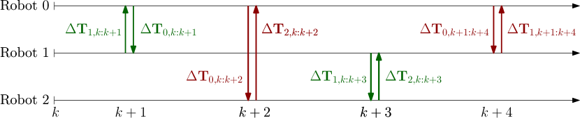
(a) Subfigure 1 list of figures text

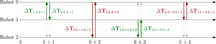
(b) Subfigure 2 list of figures text

Figure 7: Communicated RMIs with and without passive listening over a window of 4 ranging transactions, where $\Delta\mbf{T}_{i,\ell:m}$ is the RMI associated with the IMU measurements of Robot $i$ from time-step $\ell$ to time-step $m-1$.

When considering Robot 0’s perspective, the estimated relative-pose state is updated using (42) and the corresponding error covariance matrix using (43) and (61). Therefore, Robot 0 needs the IMU measurements of neighbouring robots at every time-step in order to update its estimated state of its neighbours. This is limiting since robots cannot broadcast their IMU measurements at the same rate as they are recorded due to signal interference. Additionally, to allow DS-TWR transactions to occur at the highest rate possible, the IMU information should ideally be transmitted using the ranging messages presented in Section V.

In this section, the concept of preintegration is proposed to compactly encode the IMU measurements of a neighbouring Robot $i$ over a window between two consecutive ranging instances using one relative motion increment (RMI), which is then sent over when Robot $i$ ranges with one of its neighbours. However, as illustrated in Figure 7a, without passive listening the RMIs of Robot $i$ become available to Robot 0 only when Robot 0 and Robot $i$ communicate. Given that RMIs are computed iteratively as new IMU measurements arrive, each robot needs to keep track of one RMI per neighbour. For example, looking at Figure 7a at time-step $k+3$, Robot 1 would be communicating the RMI of IMU measurements in the window $k$ to $k+3$ to Robot 1, while also tracking a separate RMI for the window starting at $k+1$ to be sent to Robot 0 at time-step $k+4$.

On the other hand, passive listening over UWB lets two actively ranging robots broadcast their RMIs to all other robots, as shown in Figure 7b. This has the advantage that IMU information of neighbours becomes available faster at all robots, and the robots computing RMIs only need to track one RMI at all times since all neighbours are up-to-date with the most recently communicated RMI.

VII-B Relative Motion Increments

Consider the case where Robot $i$ is an active robot only at non-adjacent time-steps $\ell$ and $m$. From (42), the relative pose state at time-step $m$ can be computed from the relative pose state at time-step $\ell$ as

$$\mbf{T}_{0i,m}=\left(\prod_{k=\ell}^{m-1}\mbf{U}_{0,k}\right)^{-1}\mbf{T}_{0i,\ell}\prod_{k=\ell}^{m-1}\mbf{U}_{i,k}.$$ (64)

The inputs of Robot 0 are available at Robot 0 as soon as the measurements occur, therefore the first term of (42) can be computed directly at every time-step. On the other hand, the inputs of Robot $i$ from time-step $\ell$ to $m-1$ will only be available when the robot actively shares it at time-step $m$. Rather than sharing the individual IMU measurements, Robot $i$ can simply send

$${\color[rgb]{0,0,0}\Delta\mbf{T}_{i,\ell:m}}=\prod_{k=\ell}^{m-1}\mbf{U}_{i,k}\in DE_{2}(3),$$

which is an RMI of the inputs of Robot $i$ in the window $\ell$ to $m$. The process model representing time-propagation between non-adjacent time-steps can then be rewritten as

$$\mbf{T}_{0i,m}=\left(\prod_{k=\ell}^{m-1}\mbf{U}_{0,k}\right)^{-1}\mbf{T}_{0i,\ell}\Delta\mbf{T}_{i,\ell:m}.$$ (65)

This is a feature of the process model (64) being reliant on the inputs of Robot $i$ in a separable way, meaning that the inputs of Robot $i$ can simply be post-multiplied in (64). Robot $i$ computes its RMI iteratively, starting with $\Delta\mbf{T}_{i,\ell:\ell}=\mbf{1}$, and updating it when a new input measurement arrives as

$$\Delta\mbf{T}_{i,\ell:k+1}=\Delta\mbf{T}_{i,\ell:k}\mbf{U}_{i,k}.$$ (66)

In order to linearize the RMI to be used in an EKF, a perturbation of the form

$$\Delta\mbf{T}_{i,\ell:m}=\Delta\bar{\mbf{T}}_{i,\ell:m}\operatorname{Exp}(\delta{\mbf{w}}_{i,\ell:m})$$

is defined, where $\delta{\mbf{w}}_{i,\ell m}\in\mathbb{R}^{9}$ is some unknown noise parameter associated with the RMI, which is a consequence of the noise associated with every input measurement. Despite $\Delta\mathbf{T}_{i,\ell:m}$ being an element of $DE_{2}(3)$, the above $\operatorname{Exp}$ is the exponential operator in $SE_{2}(3)$. Additionally, a right-perturbation is chosen to match the perturbation on $\mbf{U}$ derived in (60), which simplifies the subsequent derivation, but a left-perturbation could also have been chosen.

Perturbing (66) with respect to the RMI itself then yields

$$\Delta\bar{\mbf{T}}_{i,\ell:k+1}\operatorname{Exp}(\delta{\mbf{w}}_{i,\ell:k+1}) =\Delta\bar{\mbf{T}}_{i,\ell:k}\operatorname{Exp}(\delta{\mbf{w}}_{i,\ell:k})\bar{\mbf{U}}_{i,k}$$

$$=\Delta\bar{\mbf{T}}_{i,\ell:k}\bar{\mbf{U}}_{i,k}\operatorname{Exp}(\operatorname{Ad}(\bar{\mbf{U}}_{i,k}^{-1})\delta{\mbf{w}}_{i,\ell:k}),$$

which can be simplified to give

$$\delta{\mbf{w}}_{i,\ell:k+1}=\operatorname{Ad}(\bar{\mbf{U}}_{i,k}^{-1})\delta{\mbf{w}}_{i,\ell:k}.$$ (67)

Meanwhile, perturbing the RMI relative to the input noise using (60) yields

$$\Delta\bar{\mbf{T}}_{i,\ell:k+1}\operatorname{Exp}(\delta{\mbf{w}}_{i,\ell:k+1}) =\Delta\bar{\mbf{T}}_{i,\ell:k}\bar{\mbf{U}}_{i,k}\operatorname{Exp}(\mbf{L}_{i,k}\delta\mbf{u}_{i,k}),$$

which can also be simplified to give

$$\delta{\mbf{w}}_{i,\ell:k+1}=\mbf{L}_{i,k}\delta\mbf{u}_{i,k}.$$ (68)

VII-C An Asynchronous-Input Filter

Taking advantage of the separability of the process model in the neighbour’s input measurements, an asynchronous-input filter can be designed. The key idea here is to use two process models, one of the form

$$\bm{\mathcal{T}}_{0i,k+1}=\mbf{U}_{0,k}^{-1}\mbf{T}_{0i,k},\qquad\bm{\mathcal{T}}_{0i,k+1}\in DE_{2}(3)$$ (69)

at $\ell<k<m-1$ when there is no input information from Robot $i$, and another of the form

$$\mbf{T}_{0i,m}=\mbf{U}_{0,m-1}^{-1}\bm{\mathcal{T}}_{0i,m-1}\Delta\mbf{T}_{i,\ell:m}$$ (70)

when propagating from $k=m-1$ to $m$ as Robot $i$ communicates the RMI $\Delta\mbf{T}_{i,\ell:m}$. Note that $\bm{\mathcal{T}}$ denotes an intermediate state estimate that is not an element of $SE_{2}(3)$. Only when the IMU measurements of the neighbouring robot are incorporated does the estimated state restore its original $SE_{2}(3)$ form.

Given that (69) is of the same form as (42) with $\mbf{U}_{i,k}=\mbf{1}$, linearization is straightforward and follows Section VI-C,

$$\delta{\bm{\xi}}_{0i,k+1}=\operatorname{Ad}(\bar{\mbf{U}}_{0,k}^{-1})\delta{\bm{\xi}}_{0i,k}-\mbf{L}_{0,k}\delta{\mbf{u}}_{0,k}.$$ (71)

Similarly, (70) is of the same form as (42) with $\mbf{U}_{i,k}=\Delta\mbf{T}_{i,\ell:m}$, so the linearization with respect to the state is the same as (71), giving

$$\delta{\bm{\xi}}_{0i,m} =\operatorname{Ad}(\bar{\mbf{U}}_{0,m-1}^{-1})\delta{\bm{\xi}}_{0i,m-1}$$

$$\hskip 25.0pt-\mbf{L}_{0,m-1}\delta{\mbf{u}}_{0,m-1}+\operatorname{Ad}(\bar{\mbf{T}}_{0i,m})\delta{\mbf{w}}_{i,\ell:m}.$$ (72)

A summary of the proposed on-manifold EKF is shown in Algorithm 1.

Algorithm 1 Algorithm for one time-step of the proposed on-manifold EKF running on Robot 0

0:  The following is the pseudo-code for Robot 0’s EKF at time-step $k$. Let $\ell_{p}$ denote the last time Robot $p\in\{0,\ldots,n\}$ communicated with one of its neighbours. Therefore, at time-step $k-1$, Robot 0 has the RMI $\Delta\mbf{T}_{0,l_{0}:k-1}$, an intermediate estimate of neighbouring robots’ relative poses, $\hat{\bm{\mathcal{T}}}_{0q,k-1},q\in\{1,\ldots,n\}$, as well as an estimate of the relative clock states. Robot 0 additionally gets an IMU measurement, allowing it to compute $\mbf{U}_{0,k-1}$. The EKF is then as follows.

1:  Propagate RMI using $\Delta\mbf{T}_{0,l_{0}:k}=\Delta\mbf{T}_{0,l_{0}:k-1}\mbf{U}_{0,k-1}$ and its covariance using (67), (68).

2:  if ranging with neighbour $i$ then

3:     Communicate $\Delta\mbf{T}_{0,l_{0}:k}$ and its covariance.

4:     Generate 5 pseudomeasurements using (15)-(19).

5:     Propagate the relative pose state estimates in time using

$$\check{\bm{\mathcal{T}}}_{0p,k} =\mbf{U}_{0,k-1}^{-1}\hat{\bm{\mathcal{T}}}_{0p,k-1},\qquad p\in\{1,\ldots,n\},p\neq i,$$

$$\check{\mbf{T}}_{0i,k} =\mbf{U}_{0,k-1}^{-1}\hat{\bm{\mathcal{T}}}_{0i,k-1}\Delta\mbf{T}_{i,\ell_{i}:k},$$

and the clock state estimates using Section VI-D.

6:     Propagate the state-error covariances using (71), (VII-C) and Section VI-D.

7:     Do an on-manifold EKF correction step [42] using the pseudomeasurements to get $\hat{\bm{\mathcal{T}}}_{0p,k}$ and $\hat{\mbf{T}}_{0i,k}$.

8:     Initiate a new RMI $\Delta\mbf{T}_{0,k:k}=\mbf{1}$ with covariance $\mbf{0}$.

9:  else if neighbours $i$ and $j$ are ranging then

10:     Generate 8 pseudomeasurements using (15)-(19).

11:     Propagate the relative pose state estimates in time using

$$\check{\bm{\mathcal{T}}}_{0p,k} =\mbf{U}_{0,k-1}^{-1}\hat{\bm{\mathcal{T}}}_{0p,k-1},\quad p\in\{1,\ldots,n\},p\neq i,j,$$

$$\check{\mbf{T}}_{0i,k} =\mbf{U}_{0,k-1}^{-1}\hat{\bm{\mathcal{T}}}_{0i,k-1}\Delta\mbf{T}_{i,\ell_{i}:k},$$

$$\check{\mbf{T}}_{0j,k} =\mbf{U}_{0,k-1}^{-1}\hat{\bm{\mathcal{T}}}_{0j,k-1}\Delta\mbf{T}_{j,\ell_{j}:k},$$

and the clock state estimates using Section VI-D.

12:     Propagate the state-error covariances using (71), (VII-C) and Section VI-D.

13:     Do an on-manifold EKF correction step [42] using the pseudomeasurements to get $\hat{\bm{\mathcal{T}}}_{0p,k}$, $\hat{\mbf{T}}_{0i,k}$, and $\hat{\mbf{T}}_{0j,k}$.

14:  else if no one is ranging then

15:     Propagate the relative pose state estimates in time using

$$\check{\bm{\mathcal{T}}}_{0p,k} =\mbf{U}_{0,k-1}^{-1}\hat{\bm{\mathcal{T}}}_{0p,k-1},\qquad p\in\{1,\ldots,n\},$$

and the clock state estimates using Section VI-D.

16:     Propagate the state-error covariances using (71) and Section VI-D.

17:  end if

VII-D Equivalence to the No Communication Constraint Case

In the absence of communication constraint, each robot would have access to all its neighbours’ IMU measurements at all times. As explained in Section VII-A, this is not possible, so that preintegration is needed. It is shown in (65) that the state can be propagated using RMIs in a manner equivalent to the case with no communication constraint. In this subsection, it is shown that computing the uncertainty propagation for the state is also equivalent in both cases, despite the Jacobians used being different. This is in fact a consequence of the structure of the Jacobians when perturbing the state from the left.

VII-D1 No Communication Constraints

When there are no communication constraints and IMU measurements of neighbours are available at all times, the models shown in Section VI can be used to propagate the state. The covariance of the state is propagated using (43) and (61), which for two nonadjacent timestamps $\ell$ and $m$ would be written as

$$\delta{\bm{\xi}}_{0i,m}$$

$$=\operatorname{Ad}(\Delta\mbf{T}_{0,\ell:m})^{-1}\delta{\bm{\xi}}_{0i,\ell}-\sum_{k=\ell}^{m-1}\operatorname{Ad}(\Delta\mbf{T}_{0,k+1:m})^{-1}\mbf{L}_{0,k}\delta{\mbf{u}}_{0,k}$$

$$\hskip 12.0pt+\sum_{k=\ell}^{m-1}\operatorname{Ad}(\Delta\mbf{T}_{0,k+1:m}^{-1}\bar{\mbf{T}}_{0i,k+1})\mbf{L}_{i,k}\delta{\mbf{u}}_{i,k}.$$ (73)

VII-D2 With Preintegration

First, the uncertainty of the RMI can be computed using (67) and (68) as

$$\delta{\mbf{w}}_{i,\ell:m}=\sum_{k=\ell}^{m-1}\operatorname{Ad}(\Delta\mbf{T}_{i,k+1:m})^{-1}\mbf{L}_{i,k}\delta\mbf{u}_{i,k}.$$

Note that the RMI gets communicated at time-step $m$, so from timestep $\ell$ to $m-1$ the state propagation occurs only with the IMU measurements of Robot 0 as shown in (69). The uncertainty propagation from timestamp $\ell$ to $m-1$ then follows as per (71), which can be written as

$$\delta{\bm{\xi}}_{0i,m-1} =\operatorname{Ad}(\Delta\mbf{T}_{0,\ell:m-1})^{-1}\delta{\bm{\xi}}_{0i,\ell}$$

$$\hskip 12.0pt-\sum_{k=\ell}^{m-2}\operatorname{Ad}(\Delta\mbf{T}_{0,k+1:m-1})^{-1}\mbf{L}_{0,k}\delta{\mbf{u}}_{0,k}.$$

Meanwhile, propagating the uncertainty from timestamp $m-1$ to $m$ using the RMI as shown in (70) then follows as per (VII-C) to give

$$\delta{\bm{\xi}}_{0i,m}$$

$$=\operatorname{Ad}(\Delta\mbf{T}_{0,\ell:m})^{-1}\delta{\bm{\xi}}_{0i,\ell}-\sum_{k=\ell}^{m-1}\operatorname{Ad}(\Delta\mbf{T}_{0,k+1:m})^{-1}\mbf{L}_{0,k}\delta{\mbf{u}}_{0,k}$$

$$\hskip 10.0pt+\operatorname{Ad}(\Delta\mbf{T}_{0,\ell:m}^{-1}\bar{\mbf{T}}_{0i,\ell}\Delta\mbf{T}_{i,\ell:m})\delta{\mbf{w}}_{i,\ell:m}$$

$$=\operatorname{Ad}(\Delta\mbf{T}_{0,\ell:m})^{-1}\delta{\bm{\xi}}_{0i,\ell}-\sum_{k=\ell}^{m-1}\operatorname{Ad}(\Delta\mbf{T}_{0,k+1:m})^{-1}\mbf{L}_{0,k}\delta{\mbf{u}}_{0,k}$$

$$\hskip 10.0pt+\sum_{k=\ell}^{m-1}\operatorname{Ad}(\Delta\mbf{T}_{0,k+1:m}^{-1}\Delta\mbf{T}_{0,\ell:k+1}^{-1}\bar{\mbf{T}}_{0i,\ell}\Delta\mbf{T}_{i,\ell:k+1})\mbf{L}_{i,k}\delta\mbf{u}_{i,k},$$

which, using (65), simplifies to be exactly equal to (73).

VII-E Communication Requirements

The proposed multi-robot preintegration approach provides an alternative efficient way of communicating odometry information as compared to communicating the individual IMU measurements. When sending IMU measurements, no covariance information is required as the covariance matrix is typically a fixed value that can be assumed common among all robots if they all share the same kind of IMU. Meanwhile, when sending an RMI, the components of a corresponding $9\times 9$ positive-definite symmetric matrix representing its computed uncertainty must also be sent, as this is not constant but rather a function of the individual inputs.

Each IMU measurement consists of 6 single-precision floats, 3 for the gyroscope and 3 for the accelerometer readings, for a total of 24 bytes. Meanwhile, each RMI can be represented using 10 single-precision floats and the corresponding covariance matrix using the upper triangular part of the $9\times 9$ matrix, which requires communicating an additional 45 single-precision floats. Therefore, sending one RMI and its covariance matrix requires over 220 bytes of information. Therefore, unless an RMI replaces more than 9 IMU measurements, it is sometimes more efficient to communicate the raw IMU measurements. Nonetheless, using the proposed multi-robot preintegration framework has the following advantages (in addition to the discussion in Section VII-A).

• It overcomes the need for variable amount of communication, as the RMI and its covariance matrix are of fixed length but a varying number of IMU readings might be accumulated in between two instances of a robot ranging. This consequently eases implementation and provides a more reliable system.

• It provides robustness to loss of communication, as a robot re-establishing communication with its neighbours after a few seconds would not be able to send over all the accumulated IMU information.

• It reduces the amount of processing required at neighbours, as the input matrices $\mbf{U}_{i,k}$ are pre-multiplied at Robot $i$ on behalf of all its neighbours.

• It overcomes the need to know the noise distribution of the neighbours’ IMUs, which would be useful if not all robots had the same IMU.

• It allows easy integration with IMU-bias estimators and approaches that dynamically tune the covariance of the IMU measurements, without needing to send the bias estimates or the tuned covariances over UWB.

Additionally, UWB protocols by default allow 128 bytes of information to be sent per message transmission [43], for a total of 256 bytes per transceiver in each TWR instance. Given that each transceiver only needs to send 2 bytes of frame-control data per signal (thus 4 bytes of frame-control data in total) [43] and a total of 3 single-precision timestamps (thus 12 bytes of timestamps), there is enough room for the 220 bytes required to send an RMI. Note that if more information is required, some modules such as DW1000 allow up to 1024 bytes of data per message transmission [44].

VIII Simulation Results

TABLE I: Simulation parameters based on the ICM-20689 IMU and the DWM1000 UWB transceiver.

Specification	Value
Accelerometer std. dev. [m/s2]	0.023
Gyroscope std. dev. [rad/s]	0.0066
IMU rate [Hz]	250
UWB timestamping std. dev. [ns]	0.33
UWB rate [Hz]	125
Clock offset PSD [ns2/Hz]	0.4
Clock skew PSD [ppb2/Hz]	640

To evaluate the benefits of using passive listening on the estimation accuracy of relative pose states, the clock dynamics and quadcopter kinematics have been simulated. The clocks’ evolution is modelled relative to a “global time” using the simulating computer’s own clock, while the absolute-state quadcopter kinematics are simulated relative to some inertial frame. Noisy IMU and timestamp measurements are then modelled and fed into the CSRPE algorithm to estimate the relative clock and pose states.

To evaluate the proposed approach, 3 datasets are simulated.

1. S1: A single run with $n=3$ quadcopters,

2. S2: 100 Monte-Carlo trials with $n=\{2,3,4,5,6\}$, and

3. S3: 500 Monte-Carlo trials with $n=3$.

The trajectory of the quadcopters in the case of $n=2$ is shown in Figure 2, and the simulation parameters are shown in Table I. Following a periodic sequence, each pair of transceivers performs in turn a ranging transaction, except for pairs of transceivers on the same robot. The proposed algorithm is then tested on each dataset and compared to the case where no passive listening is available.

The evaluation is based on the following three criteria.

1. Accuracy: The accuracy of the proposed algorithm as compared to the case with no passive listening is quantified using error plots and the root-mean-squared-error (RMSE), which for the pose estimation error $\mbf{e}_{k}=\operatorname{Log}(\hat{\mbf{T}}_{k}\mbf{T}_{k}^{-1})$ is computed as

   $$\text{RMSE}\triangleq\sqrt{\frac{1}{N+1}\sum_{k=0}^{N}{\color[rgb]{0,0,0}\mbf{e}^{\mathsf{T}}_{k}\mbf{e}_{k}}}$$

   for $N+1$ time-steps.

2. Precision: The precision of the proposed algorithm is quantified using $\pm 3\sigma$-bound regions about the estimate, which represent a 99.73% confidence bound under a Gaussian distribution assumption.

3. Consistency: A consistent estimator is an estimator with a modelled precision that reflects the true precision of its estimate. In more specific terms, a consistent estimator outputs a covariance matrix on its estimate that is representative of the true uncertainty of that estimate. Consistency is evaluated using the normalized-estimation-error-squared (NEES) test [45, Section 5.4].

VIII-A Estimation Accuracy and Precision

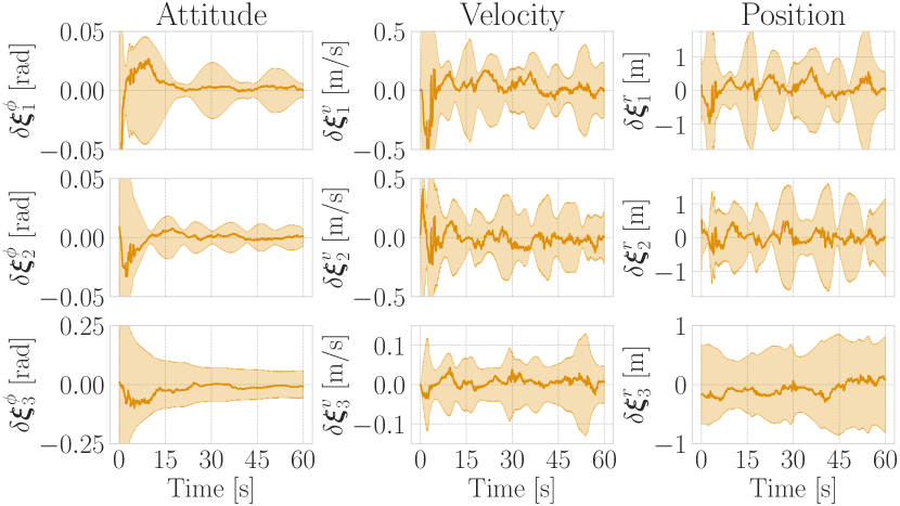
(a) Subfigure 1 list of figures text

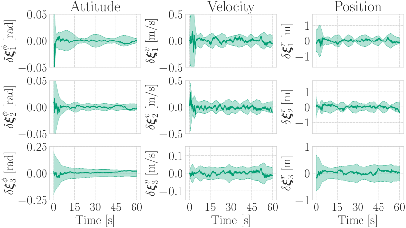
(b) Subfigure 2 list of figures text

Figure 8: Error plots and $\pm 3\sigma$ bounds (shaded region) for Robot 0’s estimate of Robot 1’s relative pose for Simulation S1.

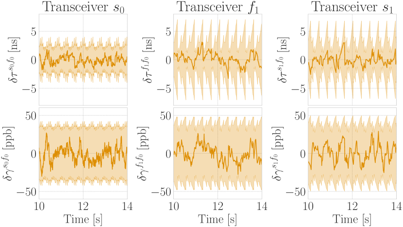
(a) Subfigure 1 list of figures text

(b) Subfigure 2 list of figures text

Figure 9: Error plots and $\pm 3\sigma$ bounds (shaded region) for Robot 0’s estimate of the clock states of Transceivers $s_{0}$, $f_{1}$, and $s_{1}$ relative to Transceiver $f_{0}$ for Simulation S1. These plots are zoomed in to a window of 4 seconds to show clearly the cycle of expanding and contracting uncertainty in the clock estimates as the transceiver alternates between active ranging and passive listening.

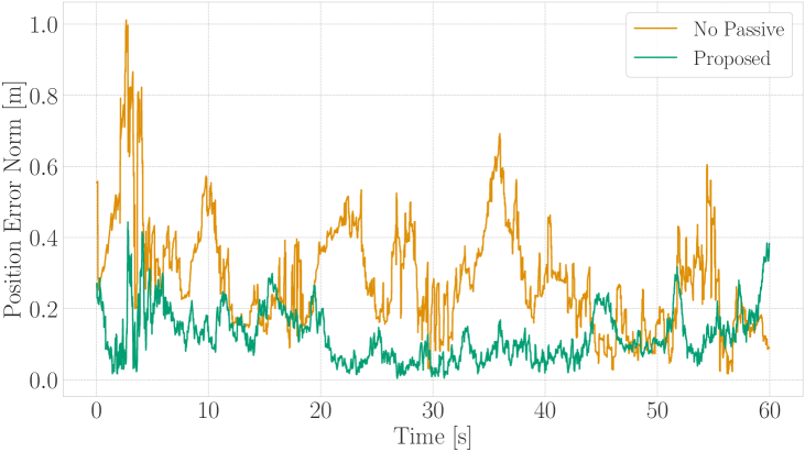
Figure 10: The error norm for Robot 0’s estimate of Robot 1’s relative pose for Simulation S1.

The error plots for the relative pose estimate of Robot 1 relative to Robot 0 in Simulation S1 are shown in Figure 8, where Figure 8a shows the error plots for the case of no passive listening and Figure 8b shows the error plots with passive listening. Passive listening reduces the positioning RMSE by 55.96% from 0.327 m to 0.144 m, and produces at almost every time-step a position error with smaller norm, as shown in Figure 10. Additionally, the estimator is significantly more confident in its estimate, as shown by the covariance bounds in Figures 8 and 9.

This improvement in localization performance can be attributed to more measurements and stronger cross-correlation between the different states when passive listening measurements are available. As shown in Figure 9, passive listening results in the clock state of a transceiver not drifting significantly in between instances where this transceiver is ranging. This brings down the clock offset RMSE of Transceiver $f_{1}$ for example by 59.31% from 1.155 ns to 0.470 ns.

The improvement in performance can also be seen as the number of robots is increased, as shown in Table II for the Simulation S2. Because only one pair of transceivers can communicate at a time, in the absence of passive listening the rate at which each transceiver participates in a ranging transaction decreases with the number of transceivers, and as a result the overall localization performance degrades. With passive listening on the other hand, adding robots does not result in longer periods without measurements and the measurement rate per robot remains the same. In fact, it turns out that adding robots in the presence of passive listening produces better performance due to spatial variations in the range-measurement sources [46].

To provide further insight into the contribution of passive listening measurements on the behaviour of the estimator, the distribution of the RMSEs of the position and attitude estimates of all robots in Simulation S3 are visualized in Figure 11.

TABLE II: The average RMSE (aRMSE) of Robot 0’s estimate of neighbouring robots’ relative pose for Simulation S2.

	Robot 1			Robot 2			Average for all robots
Number of Robots	No Passive aRMSE [m]	Proposed aRMSE [m]	Change [%]	No Passive aRMSE [m]	Proposed aRMSE [m]	Change [%]	No Passive aRMSE [m]	Proposed aRMSE [m]	Change [%]
3	0.527	0.266	-49.53	0.445	0.261	-41.35	0.486	0.263	-45.88
4	0.673	0.209	-68.95	0.531	0.203	-61.77	0.574	0.222	-61.32
5	0.967	0.220	-77.25	0.652	0.201	-69.17	0.662	0.211	-68.13
6	1.270	0.212	-83.31	0.780	0.197	-74.74	0.737	0.199	-73.00
7	1.683	0.198	-88.24	0.892	0.172	-80.72	0.917	0.165	-82.01

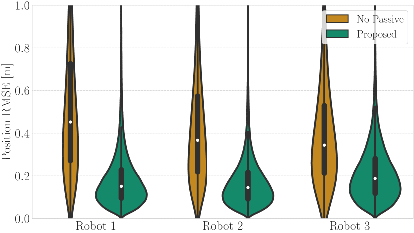
(a) Subfigure 1 list of figures text

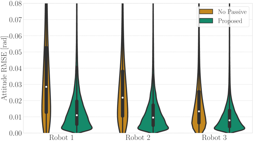
(b) Subfigure 2 list of figures text

Figure 11: Violin and box plots showing the distribution of the position and attitude RMSEs for Simulation S3. The envelope shows the relative frequency of RMSE values. The box plot shows the median as a white dot, while the first and third quartile of the data are represented using the lower and upper bound of the thick black bar, respectively.

VIII-B Consistency

Given that the estimator is an EKF, consistency cannot be guaranteed due to linearization and discretization errors. Nonetheless, the proposed on-manifold framework can characterize banana-shaped error distributions that result from range measurements as shown in Figure 3 more efficiently. Consequently, the error distribution appears to be well-characterized by the estimator as shown in Figures 8 and 9, as the error trajectory typically lies within the $\pm 3\sigma$ bounds.

A better evaluation of the consistency of the estimator is a NEES test, which is performed over the 500 trials of Simulation S3 and is shown in Figure 12. During the first few seconds when the quadcopters are taking off from the ground, their geometry and low speeds result in a weakly-observable system [37], which results in overconfidence of the estimator as linearization-based filters can correct in unobservable directions [47, 48]. Nonetheless, the estimator then converges towards consistency, although it is never perfectly consistent due to linearization and discretization errors, which is a feature of EKFs. This can be solved by slightly inflating the associated covariance matrices used in the filter.

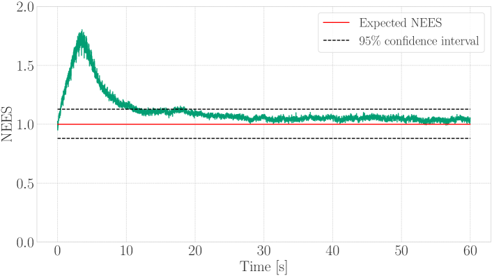
Figure 12: 500-trial NEES plot for the proposed estimator on Simulation S3.

IX Experimental Results

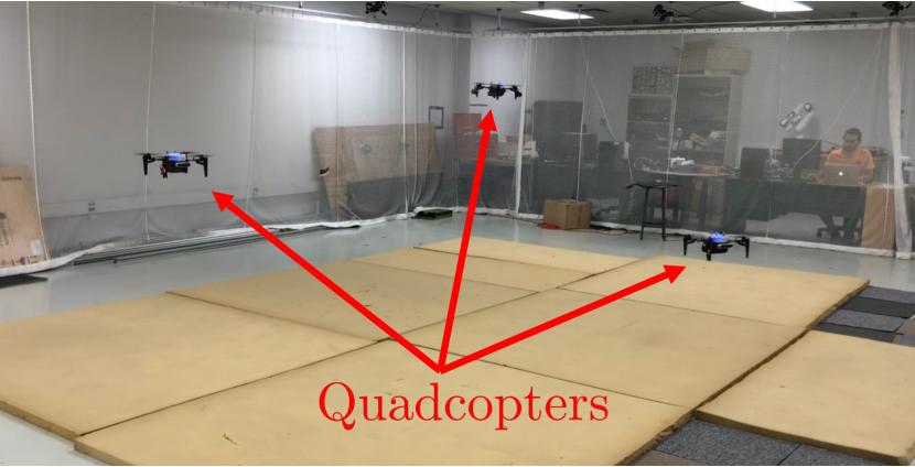
Figure 13: (Left) 3 quadcopters in the experimental space. (Middle) The experimental trajectory for Trial 1, where each colour represents the trajectory of a different quadcopter and the grid represents a roughly 5 m $\times$ 5 m area. (Right) The experimental trajectory for Trial 2.

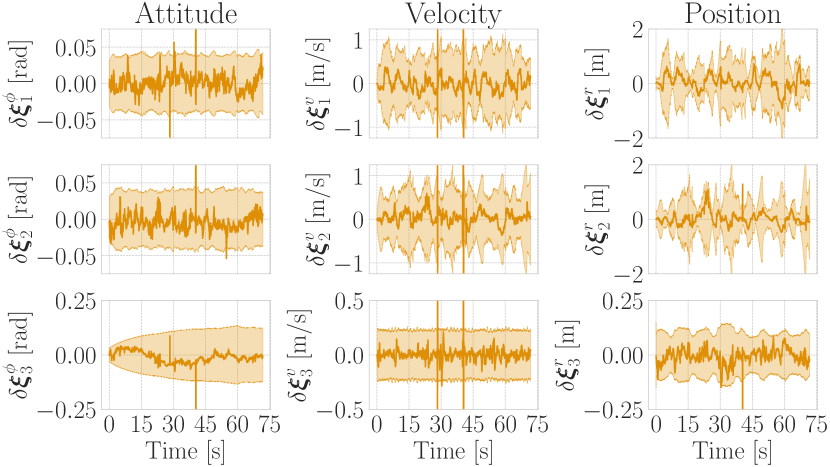
(a) Subfigure 1 list of figures text

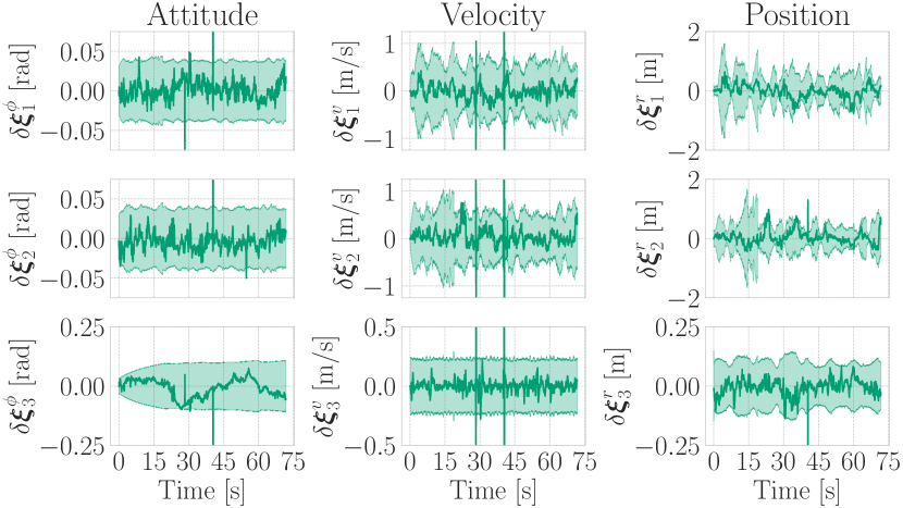
(b) Subfigure 2 list of figures text

Figure 14: Error plots and $\pm 3\sigma$ bounds (shaded region) for Robot 0’s estimate of Robot 1’s relative pose for experimental trial 1.

The proposed approach is tested on multiple experimental trials. The ranging protocol discussed in Section V is implemented in C on custom-made boards fitted with DWM1000 UWB transceivers [44]. Two boards are then fitted to Uvify IFO-S quadcopters approximately 45 cm apart. The experimental set-up is shown in Figure 1. Three of these quadcopters are then used for the experimental results shown in this section, with multiple approximately-minute-long trajectories similar to the one shown in Figure 13 in a roughly 5 m $\times$ 5 m area. In order to analyze the error in the pose estimates of the robots, a 12-camera Vicon motion-capture system is used to record the ground-truth pose of each quadcopter.

To enable the 6 transceivers to take turn ranging with one another, the common-list protocol discussed in Section V is implemented using robot operating system (ROS). This allows each robot to range with its neighbours at a rate of 90 Hz, and collect passive listening measurements at a rate of 150 Hz. These UWB measurements are corrected for antenna delays and power-induced biases using [6], before fusing them with the onboard IMU and height measurements in the proposed EKF. An ICM-20689 IMU is used with characteristics similar to the simulated ones given in Table I, and the height measurements are obtained from a downward-facing camera. The height measurement error is assumed Gaussian with 5 cm of standard deviation. To reject outliers in the range and passive-listening measurements, the normalized-innovation-squared (NIS) test is implemented in the filter [45, Section 5.4].

The pose-error plots for one of the trials are shown in Figure 14 with and without fusing passive listening measurements, and the RMSE comparison for 4 different trials with varying motion are shown in Table III. Even though both scenarios result in error trajectories that fall within the error bounds, it is clear that with the additional passive listening measurements available to the robot at 150 Hz, the relative position estimates in particular become significantly less uncertain. Additionally, these error plots correspond to the first row in Table III, showing that the improvement in the confidence of the estimator is additionally accompanied with a 26.83% and 14.89% reduction in the RMSE for Robot 1’s and Robot 2’s position RMSE, respectively. This reduction in RMSE goes up to 55.81% for one of the runs when passive listening measurements are utilized.

TABLE III: The RMSE of Robot 0’s estimate of neighbouring robots’ relative pose for multiple experimental trials.

	Robot 1			Robot 2
	No Passive RMSE [m]	Proposed RMSE [m]	Change [%]	No Passive RMSE [m]	Proposed RMSE [m]	Change [%]
Trial 1	0.518	0.379	-26.83	0.356	0.303	-14.89
Trial 2	1.079	0.641	-40.59	0.828	0.511	-38.29
Trial 3	0.603	0.475	-21.23	0.583	0.410	-29.67
Trial 4	1.007	0.445	-55.81	0.711	0.465	-34.60

X Conclusion

In this paper, the problem of relative extended pose estimation has been addressed for a team of robots each equipped with UWB transceivers. A novel ranging protocol is proposed that allows neighbouring robots to passively listen-in on the measurements without any underlying assumptions on the hierarchy of the communication. This is then utilized to implement a simple MAC protocol and an efficient means for sharing preintegrated IMU information, which is then fused with the UWB measurements in a filter that estimates both the clock states of the transceivers and the relative poses of the robots. The relative poses and the preintegration are formulated directly on $SE_{2}(3)$. This is then all evaluated in simulation using different numbers of robots and Monte-Carlo trials, and in experiments using multiple trials of 3 quadcopters each equipped with 2 UWB transceivers. The method is shown to improve the localization performance significantly when compared to the case of no passive listening measurements.

This work can be extended to address complications that arise in wireless communication, such as packet drop. When a packet drop occurs, neighbours miss an RMI which is required to propagate their estimates forward, and therefore this must be addressed in a real-world application, potentially by providing a means for robots to request a missed RMI from their neighbours. Future work will additionally consider more efficient scheduling schemes where only a subset of the transceivers range with one another in pairs while the remaining transceivers are always passively listening. Other potential extensions of this paper include addressing dynamic graphs, incomplete graphs, and collaboration between robots, as robots can share their state estimates with neighbours to reach a consensus on the clock and relative pose states.

Appendix A Fold Increase in Measurements

When there are $n+1$ robots and 2 transceivers per robot, the total number of transceivers is $n_{t}=2(n+1)$. Therefore, the number of ranging pairs with transceivers on distinct robots is

$$n_{\text{p}} =\frac{2(n+1)(2(n+1)-1)}{2}-(n+1)=2n(n+1).$$

The number of direct measurements between all robots is then 2$n_{\text{p}}$ (one range and one offset measurement per pair), while the number of passive listening measurements recorded at all robots is $n_{\text{p}}(3(n_{\text{t}}-2))=6nn_{\text{p}}$. Therefore, the fold increase in measurements is

$$\frac{2n_{\text{p}}+6nn_{\text{p}}}{2n_{\text{p}}}=1+3n$$

when considering a centralized approach where passive listening measurements from all robots are available.

A similar analysis can be done from the perspective of one robot that does not have access to passive listening measurements recorded at neighbouring robots. Without passive listening it can be shown that the robot only gets $8n$ distinct measurements, while with listening-in on neighbouring robots’ messages the robot gets $2n_{\text{p}}-8n$ new measurements from the direct measurements between the neighbours and $12n^{2}$ new passive listening measurements. This can be shown to be a $(\frac{1}{2}+2n)$-fold increase in the number of measurements from the individual robot’s perspective.

Appendix B Linearizing the Range Measurement Model

Consider as in (14) an expression of the form

$$d =\left\|\Big{(}\tilde{\mbf{1}}\big{(}\mbf{T}_{2}\tilde{\mbf{r}}_{2}-\mbf{T}_{1}\tilde{\mbf{r}}_{1}\big{)}\Big{)}\right\|,$$ (74)

where $\mbf{T}_{1},\mbf{T}_{2}\in SE(3)$ and $\mbf{r}_{1},\mbf{r}_{2}\in\mathbb{R}^{5}$. Squaring both sides and perturbing the measurement and the pose states yields

$$(\bar{d}+\delta{d})^{2} =\Big{(}\tilde{\mbf{1}}\big{(}\operatorname{Exp}(\delta{\bm{\xi}}_{2})\bar{\mbf{T}}_{2}\tilde{\mbf{r}}_{2}-\operatorname{Exp}(\delta{\bm{\xi}}_{1})\bar{\mbf{T}}_{1}\tilde{\mbf{r}}_{1}\big{)}\Big{)}^{\mathsf{T}}\Big{(}\cdot\Big{)},$$

which, using (2), can be expanded to give

$$\bar{d}^{2}+2\bar{d}\delta{d} \approx(\tilde{\mbf{1}}\bar{\mbf{T}}_{2}\tilde{\mbf{r}}_{2})^{\mathsf{T}}\tilde{\mbf{1}}\bar{\mbf{T}}_{2}\tilde{\mbf{r}}_{2}+(\tilde{\mbf{1}}\bar{\mbf{T}}_{1}\tilde{\mbf{r}}_{1})^{\mathsf{T}}\tilde{\mbf{1}}\bar{\mbf{T}}_{1}\tilde{\mbf{r}}_{1}$$

$$\hskip 12.0pt-(\tilde{\mbf{1}}\bar{\mbf{T}}_{2}\tilde{\mbf{r}}_{2})^{\mathsf{T}}\tilde{\mbf{1}}\bar{\mbf{T}}_{1}\tilde{\mbf{r}}_{1}-(\tilde{\mbf{1}}\bar{\mbf{T}}_{1}\tilde{\mbf{r}}_{1})^{\mathsf{T}}\tilde{\mbf{1}}\bar{\mbf{T}}_{2}\tilde{\mbf{r}}_{2}$$

$$\hskip 12.0pt-(\tilde{\mbf{1}}\delta{\bm{\xi}}_{2}^{\wedge}\bar{\mbf{T}}_{2}\tilde{\mbf{r}}_{2})^{\mathsf{T}}\tilde{\mbf{1}}\bar{\mbf{T}}_{1}\tilde{\mbf{r}}_{1}-(\tilde{\mbf{1}}\bar{\mbf{T}}_{2}\tilde{\mbf{r}}_{2})^{\mathsf{T}}\tilde{\mbf{1}}\delta{\bm{\xi}}_{1}^{\wedge}\bar{\mbf{T}}_{1}\tilde{\mbf{r}}_{1}$$

$$\hskip 12.0pt-(\tilde{\mbf{1}}\delta{\bm{\xi}}_{1}^{\wedge}\bar{\mbf{T}}_{1}\tilde{\mbf{r}}_{1})^{\mathsf{T}}\tilde{\mbf{1}}\bar{\mbf{T}}_{2}\tilde{\mbf{r}}_{2}-(\tilde{\mbf{1}}\bar{\mbf{T}}_{1}\tilde{\mbf{r}}_{1})^{\mathsf{T}}\tilde{\mbf{1}}\delta{\bm{\xi}}_{2}^{\wedge}\bar{\mbf{T}}_{2}\tilde{\mbf{r}}_{2},$$

where higher order terms have been neglected. Cancelling out the nominal terms on both sides, using the fact that each term is scalar, and recalling (1),

$$2\bar{d}\delta{d}=-2(\tilde{\mbf{1}}\bar{\mbf{T}}_{2}\tilde{\mbf{r}}_{2})^{\mathsf{T}}\tilde{\mbf{1}}\delta{\bm{\xi}}_{1}^{\wedge}\bar{\mbf{T}}_{1}\tilde{\mbf{r}}_{1}-2(\tilde{\mbf{1}}\bar{\mbf{T}}_{1}\tilde{\mbf{r}}_{1})^{\mathsf{T}}\tilde{\mbf{1}}\delta{\bm{\xi}}_{2}^{\wedge}\bar{\mbf{T}}_{2}\tilde{\mbf{r}}_{2}$$

$$\;\;=-2(\tilde{\mbf{1}}^{\mathsf{T}}\tilde{\mbf{1}}\bar{\mbf{T}}_{2}\tilde{\mbf{r}}_{2})^{\mathsf{T}}(\bar{\mbf{T}}_{1}\tilde{\mbf{r}}_{1})^{\odot}\delta{\bm{\xi}}_{1}-2(\tilde{\mbf{1}}^{\mathsf{T}}\tilde{\mbf{1}}\bar{\mbf{T}}_{1}\tilde{\mbf{r}}_{1})^{\mathsf{T}}(\bar{\mbf{T}}_{2}\tilde{\mbf{r}}_{2})^{\odot}\delta{\bm{\xi}}_{2}.$$

Therefore, the linearized model for (74) is

$$\delta{d} =-\frac{1}{\bar{d}}(\tilde{\mbf{1}}^{\mathsf{T}}\tilde{\mbf{1}}\bar{\mbf{T}}_{2}\tilde{\mbf{r}}_{2})^{\mathsf{T}}(\bar{\mbf{T}}_{1}\tilde{\mbf{r}}_{1})^{\odot}\delta{\bm{\xi}}_{1}$$

$$\hskip 12.0pt-\frac{1}{\bar{d}}(\tilde{\mbf{1}}^{\mathsf{T}}\tilde{\mbf{1}}\bar{\mbf{T}}_{1}\tilde{\mbf{r}}_{1})^{\mathsf{T}}(\bar{\mbf{T}}_{2}\tilde{\mbf{r}}_{2})^{\odot}\delta{\bm{\xi}}_{2}.$$

Appendix C Discretizing the Input Matrix

The matrices $\tilde{\mbf{U}}_{0,k}$ and $\tilde{\mbf{U}}_{i,k}$ in (42) are of the general form

$$\tilde{\mbf{U}}=\left[\begin{array}[]{cc}\mbf{u}^{\wedge}&\mbf{e}_{4}\\ \mbf{0}_{{\color[rgb]{0,0,0}1\times 4}}&0\end{array}\right],$$ (75)

where $\mbf{u}=\left[\begin{array}[]{cc}\bm{\omega}^{\mathsf{T}}&\bm{\alpha}^{\mathsf{T}}\end{array}\right]^{\mathsf{T}}$, $(\cdot)^{\wedge}$ is the wedge operator in $SE(3)$, and $\mbf{e}_{4}=\left[\begin{array}[]{cc}\mbf{0}_{{\color[rgb]{0,0,0}1\times 3}}&1\end{array}\right]^{\mathsf{T}}$. Consequently,

$$\mbf{U} =\operatorname{exp}(\tilde{\mbf{U}}\Delta t)=\sum_{\ell=0}^{\infty}\frac{1}{\ell!}\left(\mbf{U}\Delta t\right)^{\ell}$$

$$=\mbf{1}+\left[\begin{array}[]{cc}\mbf{u}^{\wedge}&\mbf{e}_{4}\\ \mbf{0}&0\end{array}\right]\Delta t+\frac{1}{2!}\left[\begin{array}[]{cc}(\mbf{u}^{\wedge})^{2}&\mbf{u}^{\wedge}\mbf{e}_{4}\\ \mbf{0}&0\end{array}\right](\Delta t)^{2}$$ (80)

$$\hskip 12.0pt+\frac{1}{3!}\left[\begin{array}[]{cc}(\mbf{u}^{\wedge})^{3}&(\mbf{u}^{\wedge})^{2}\mbf{e}_{4}\\ \mbf{0}&0\end{array}\right](\Delta t)^{3}+\ldots$$ (83)

$$=\left[\begin{array}[]{cc}\sum_{\ell=0}^{\infty}\frac{1}{\ell!}(\mbf{u}^{\wedge}\Delta t)^{\ell}&\sum_{\ell=0}^{\infty}\frac{1}{(\ell+1)!}(\mbf{u}^{\wedge}\Delta t)^{\ell}\mbf{e}_{4}\Delta t\\ \mbf{0}&1\end{array}\right].$$ (86)

Note that $\sum_{\ell=0}^{\infty}\frac{1}{\ell!}(\mbf{u}^{\wedge}\Delta t)^{\ell}=\operatorname{Exp}(\mbf{u}\Delta t)$, where $\operatorname{Exp}$ is the $SE(3)$ exponential operator, giving

$$\sum_{\ell=0}^{\infty}\frac{1}{\ell!}(\mbf{u}^{\wedge}\Delta t)^{\ell}=\left[\begin{array}[]{cc}\operatorname{Exp}(\bm{\omega}\Delta t)&\mbf{J}_{l}(\bm{\omega}\Delta t)\bm{\alpha}\\ \mbf{0}&1\end{array}\right],$$ (87)

and

$$\mbf{J}_{l}(\bm{\psi}) =\sum_{\ell=0}^{\infty}\frac{1}{(\ell+1)!}\left(\phi\bm{\phi}^{\times}\right)^{\ell}$$

$$=\frac{\operatorname{sin}\phi}{\phi}\mbf{1}+\left(1-\frac{\operatorname{sin}\phi}{\phi}\right)\bm{\phi}\bm{\phi}^{\mathsf{T}}+\frac{1-\operatorname{cos}\phi}{\phi}\bm{\phi}^{\times}$$

is the left Jacobian of $SO(3)$, where $\phi=|\bm{\psi}|$ and $\bm{\phi}=\bm{\psi}/\phi$. Meanwhile,

$$\sum_{\ell=0}^{\infty}\frac{1}{(\ell+1)!}(\mbf{u}^{\wedge}\Delta t)^{\ell}$$

$$=\mbf{1}+\frac{1}{2!}\left[\begin{array}[]{cc}\bm{\omega}^{\times}&\bm{\alpha}\\ \mbf{0}&0\end{array}\right]\Delta t+\frac{1}{3!}\left[\begin{array}[]{cc}(\bm{\omega}^{\times})^{2}&\bm{\omega}^{\times}\bm{\alpha}\\ \mbf{0}&0\end{array}\right](\Delta t)^{2}$$ (92)

$$\hskip 12.0pt+\frac{1}{4!}\left[\begin{array}[]{cc}(\bm{\omega}^{\times})^{3}&(\bm{\omega}^{\times})^{2}\bm{\alpha}\\ \mbf{0}&0\end{array}\right](\Delta t)^{3}+\ldots$$ (95)

$$=\left[\begin{array}[]{cc}\sum_{\ell=0}^{\infty}\frac{1}{(\ell+1)!}(\bm{\omega}^{\times}\Delta t)^{\ell}&\sum_{\ell=0}^{\infty}\frac{1}{(\ell+2)!}(\bm{\omega}^{\times}\Delta t)^{\ell}\bm{\alpha}\Delta t\\ \mbf{0}&1\end{array}\right]$$ (98)

$$=\left[\begin{array}[]{cc}\mbf{J}_{l}(\bm{\omega}\Delta t)&\frac{\Delta t}{2}\mbf{N}_{l}(\bm{\omega}\Delta t)\bm{\alpha}\\ \mbf{0}&1\end{array}\right],$$ (101)

where

$$\mbf{N}(\bm{\psi}) =2\sum_{\ell=0}^{\infty}\frac{1}{(\ell+2)!}\left(\phi\bm{\phi}^{\times}\right)^{\ell}$$

$$=\bm{\phi}\bm{\phi}^{\mathsf{T}}+2\left(\frac{1}{\phi}-\frac{\operatorname{sin}\phi}{\phi^{2}}\right)\bm{\phi}^{\times}+2\frac{\operatorname{cos}\phi-1}{\phi^{2}}\bm{\phi}^{\times}\bm{\phi}^{\times}.$$

Substituting (87) and (101) back into (86) gives

$$\mbf{U}=\left[\begin{array}[]{ccc}\operatorname{Exp}(\bm{\omega}\Delta t)&\mbf{J}_{l}(\bm{\omega}\Delta t)\bm{\alpha}&\frac{\Delta t^{2}}{2}\mbf{N}_{l}(\bm{\omega}\Delta t)\bm{\alpha}\\ &1&\Delta t\\ &&1\end{array}\right].$$ (102)

Appendix D Biography Section

Mohammed Ayman Shalaby (Student Member, IEEE) received the B.Eng. degree in Mechanical Engineering from McGill University, Montreal, QC, Canada in 2019. He is currently a Ph.D. Candidate at McGill University. His research interests include state estimation, multi-robot systems, and ultra-wideband communication, with applications to autonomous navigation of robotic systems.

Charles Champagne Cossette (Student Member, IEEE) is a Ph.D. Candidate at McGill University. Charles is currently working on state estimation and planning for multi-robot teams using ultra-wideband radio.

Jerome Le Ny (Senior Member, IEEE) received the Ph.D. degree in Aeronautics and Astronautics from the Massachusetts Institute of Technology, Cambridge, in 2008. He is currently an Associate Professor with the Department of Electrical Engineering, Polytechnique Montreal, Canada, and a member of GERAD, a multi-university research center on decision analysis. From 2008 to 2012 he was a Postdoctoral Researcher with the GRASP Laboratory at the University of Pennsylvania. In 2018-2019, he was an Alexander von Humboldt Fellow at the Technical University of Munich. His research interests include robust and stochastic control, mean-field control, networked control systems, dynamic resource allocation problems, privacy and security in sensor and actuator networks, with applications to autonomous multi-robot systems and intelligent infrastructure systems. He currently serves as an Associate Editor for the IEEE Transactions on Robotics.

James Richard Forbes (Member, IEEE) received the B.A.Sc. degree in Mechanical Engineering (Honours, Co-op) from the University of Waterloo, Waterloo, ON, Canada in 2006, and the M.A.Sc. and Ph.D. degrees in Aerospace Science and Engineering from the University of Toronto Institute for Aerospace Studies (UTIAS), Toronto, ON, Canada in 2008 and 2011, respectively. James is currently an Associate Professor and William Dawson Scholar in the Department of Mechanical Engineering at McGill University, Montreal, QC, Canada. James is a Member of the Centre for Intelligent Machines (CIM), a Member of the Group for Research in Decision Analysis (GERAD), and a Member of the Trottier Institute for Sustainability in Engineering and Design (TISED). James was awarded the McGill Association of Mechanical Engineers (MAME) Professor of the Year Award in 2016, the Engineering Class of 1944 Outstanding Teaching Award in 2018, and the Carrie M. Derick Award for Graduate Supervision and Teaching in 2020. The focus of James’ research is navigation, guidance, and control of robotic systems. James is currently an Associate Editor of the International Journal of Robotics Research (IJRR).

References

- [1] C. Forster, L. Carlone, F. Dellaert, and D. Scaramuzza, “On-Manifold Preintegration for Real-Time Visual-Inertial Odometry,” IEEE Trans. on Robotics, vol. 33, no. 1, pp. 1–21, 2017.
- [2] M. Kok, J. D. Hol, and T. B. Schon, “Indoor positioning using ultrawideband and inertial measurements,” IEEE Trans. on Vehicular Technology, vol. 64, no. 4, pp. 1293–1303, 2015.
- [3] M. W. Mueller, M. Hamer, and R. D’Andrea, “Fusing ultra-wideband range measurements with accelerometers and rate gyroscopes for quadrocopter state estimation,” IEEE Int. Conf. on Robotics and Automation, pp. 1730–1736, 2015.
- [4] R. Jung and S. Weiss, “Scalable and modular ultra-wideband aided inertial navigation,” in IEEE/RSJ International Conference on Intelligent Robots and Systems (IROS), 2022, pp. 2423–2430.
- [5] D. Neirynck, E. Luk, and M. McLaughlin, “An alternative double-sided two-way ranging method,” Workshop on Positioning, Navigation and Communication, pp. 16–19, 2017.
- [6] M. A. Shalaby, C. C. Cossette, J. R. Forbes, and J. Le Ny, “Calibration and Uncertainty Characterization for Ultra-Wideband Two-Way-Ranging Measurements,” arXiv: 2210.05888 [cs.ro], 2022.
- [7] P. Groves, Principles of GNSS, Inertial, and Multisensor Integrated Navigation Systems, Second Edition. Artech House Publishers, 2013.
- [8] K. A. Horvath, G. Ill, and A. Milankovich, “Passive extended double-sided two-way ranging algorithm for UWB positioning,” Int. Conf. on Ubiquitous and Future Networks, pp. 482–487, 2017.
- [9] S. Shah and T. Demeechai, “Multiple simultaneous ranging in IR-UWB networks,” Sensors, vol. 19, no. 24, pp. 1–14, 2019.
- [10] T. Laadung, S. Ulp, M. M. Alam, and Y. L. Moullec, “Novel Active-Passive Two-Way Ranging Protocols for UWB Positioning Systems,” IEEE Sensors Journal, vol. 22, no. 6, pp. 5223–5237, 2022.
- [11] A. Ledergerber, M. Hamer, and R. D’Andrea, “A robot self-localization system using one-way ultra-wideband communication,” IEEE Int. Conf. on Intelligent Robots and Systems, pp. 3131–3137, 2015.
- [12] M. Hamer and R. D’andrea, “Self-Calibrating Ultra-Wideband Network Supporting Multi-Robot Localization,” IEEE Access, vol. 6, pp. 22 292–22 304, 2018.
- [13] R. Zandian and U. Witkowski, “Robot Self-Localization in Ultra-Wideband Large Scale Multi-Node Setups,” Workshop on Positioning, Navigation and Communications (WPNC), 2017.
- [14] J. Cano, S. Chidami, and J. Le Ny, “A Kalman Filter-Based Algorithm for Simultaneous Time Synchronization and Localization in UWB Networks,” in Int. Conf. on Robotics and Automation (ICRA), 2019, pp. 1431–1437.
- [15] D. E. Badawy, V. Larsson, M. Pollefeys, and I. Dokmanić, “Localizing Unsynchronized Sensors with Unknown Sources,” arXiv: 2102.03565 [eess.SP], 2021.
- [16] A. Alanwar, H. Ferraz, K. Hsieh, R. Thazhath, P. Martin, J. Hespanha, and M. Srivastava, “D-SLATS: Distributed simultaneous localization and time synchronization,” Int. Symposium on Mobile Ad Hoc Networking and Computing (MobiHoc), 2017.
- [17] T. M. Nguyen, T. H. Nguyen, M. Cao, Z. Qiu, and L. Xie, “Integrated UWB-vision approach for autonomous docking of UAVS in GPS-denied environments,” IEEE Int. Conf. on Robotics and Automation, pp. 9603–9609, 2019.
- [18] H. Xu, L. Wang, Y. Zhang, K. Qiu, and S. Shen, “Decentralized Visual-Inertial-UWB Fusion for Relative State Estimation of Aerial Swarm,” IEEE Int. Conf. on Robotics and Automation, pp. 8776–8782, 2020.
- [19] R. Jung and S. Weiss, “Scalable Recursive Distributed Collaborative State Estimation for Aided Inertial Navigation,” in Int. Conf. on Robotics and Automation (ICRA), 2021.
- [20] Q. Shi, X. Cui, S. Zhao, and M. Lu, “Sequential TOA-Based Moving Target Localization in Multi-Agent Networks,” IEEE Communications Letters, vol. 24, no. 8, pp. 1719–1723, 2020.
- [21] M. Shalaby, C. C. Cossette, J. R. Forbes, and J. Le Ny, “Relative Position Estimation in Multi-Agent Systems Using Attitude-Coupled Range Measurements,” IEEE Robotics and Automation Letters, vol. 6, no. 3, pp. 4955–4961, 2021.
- [22] T. M. Nguyen, A. H. Zaini, C. Wang, K. Guo, and L. Xie, “Robust Target-Relative Localization with Ultra-Wideband Ranging and Communication,” IEEE Int. Conf. on Robotics and Automation, pp. 2312–2319, 2018.
- [23] B. Hepp, T. Nägeli, and O. Hilliges, “Omni-directional person tracking on a flying robot using occlusion-robust ultra-wideband signals,” IEEE Int. Conf. on Intelligent Robots and Systems, pp. 189–194, 2016.
- [24] Q. Shi, X. Cui, S. Zhao, S. Xu, and M. Lu, “BLAS: Broadcast relative localization and clock synchronization for dynamic dense multiagent systems,” IEEE Trans. on Aerospace and Electronic Systems, vol. 56, no. 5, pp. 3822–3839, 2020.
- [25] Z. Dou, Z. Yao, and M. Lu, “Asynchronous Collaborative Localization System for Large-Capacity Sensor Networks,” IEEE Internet of Things Journal, vol. 9, no. 16, pp. 15 349–15 361, 2022.
- [26] M. Shalaby, C. C. Cossette, J. Le Ny, and J. R. Forbes, “Cascaded Filtering Using the Sigma Point Transformation,” IEEE Robotics and Automation Letters, vol. 6, no. 3, pp. 4758–4765, 2021.
- [27] E. Allak, R. Jung, and S. Weiss, “Covariance Pre-Integration for Delayed Measurements in Multi-Sensor Fusion,” IEEE Int. Conf. on Intelligent Robots and Systems, pp. 6642–6649, 2019.
- [28] E. Allak, A. Barrau, R. Jung, J. Steinbrener, and S. Weiss, “Centralized-equivalent pairwise estimation with asynchronous communication constraints for two robots,” in IEEE/RSJ International Conference on Intelligent Robots and Systems (IROS), 2022, pp. 8544–8551.
- [29] T. Lupton and S. Sukkarieh, “Visual-inertial-aided navigation for high-dynamic motion in built environments without initial conditions,” IEEE Trans. on Robotics, vol. 28, no. 1, pp. 61–76, 2012.
- [30] A. Barrau and S. Bonnabel, “Linear observed systems on groups,” Systems and Control Letters, no. 129, pp. 36–42, 2019.
- [31] M. Brossard, A. Barrau, P. Chauchat, and S. Bonnabel, “Associating Uncertainty to Extended Poses for on Lie Group IMU Preintegration With Rotating Earth,” IEEE Trans. on Robotics, pp. 1–16, 2021.
- [32] J. González, J. L. Blanco, C. Galindo, A. Ortiz-de Galisteo, J. A. Fernández-Madrigal, F. A. Moreno, and J. L. Martínez, “Mobile robot localization based on Ultra-Wide-Band ranging: A particle filter approach,” Robotics and Autonomous Systems, vol. 57, no. 5, pp. 496–507, 2009.
- [33] R. Liu, C. Yuen, T. N. Do, D. Jiao, X. Liu, and U. X. Tan, “Cooperative relative positioning of mobile users by fusing IMU inertial and UWB ranging information,” IEEE Int. Conf. on Robotics and Automation, pp. 5623–5629, 2017.
- [34] A. W. Long, C. K. Wolfe, M. J. Mashner, and G. S. Chirikjian, “The banana distribution is Gaussian: A localization study with exponential coordinates,” Robotics: Science and Systems, vol. 8, pp. 265–272, 2013.
- [35] T. D. Barfoot, State Estimation for Robotics, Second Edition. Cambridge University Press, 2022.
- [36] LAN/MAN Standards Committee, “Part 15.4: wireless medium access control (MAC) and physical layer (PHY) specifications for low-rate wireless personal area networks (LR-WPANs),” IEEE Computer Society, 2003.
- [37] C. C. Cossette, M. Shalaby, D. Saussie, J. R. Forbes, and J. Le Ny, “Relative Position Estimation between Two UWB Devices with IMUs,” IEEE Robotics and Automation Letters, vol. 6, no. 3, pp. 4313–4320, 2021.
- [38] M. A. Shalaby, C. Champagne Cossette, J. R. Forbes, and J. Le Ny, “Reducing Two-way Ranging Variance by Signal-Timing Optimization,” arXiv: 2211.00538 [eess.SP], 2022.
- [39] A. V. Rao, Dynamics of Particles and Rigid Bodies: A Systematic Approach. Cambridge University Press, 2006.
- [40] M. Behr, P. Benner, and J. Heiland, “Solution formulas for differential Sylvester and Lyapunov equations,” Calcolo, vol. 56, no. 4, pp. 1–33, 2019.
- [41] J. A. Farrell, Aided Navigation: GPS with High Rate Sensors. McGraw-Hill, 2008.
- [42] J. Solà, J. Deray, and D. Atchuthan, “A micro Lie theory for state estimation in robotics,” arXiv: 1812.01537 [cs.Ro], 2018.
- [43] IEEE Computer Society, “IEEE Standard for Low-Rate Wireless Networks. Amendment 1: Add Alternate PHYs (IEEE Std 802.15.4a),” IEEE Software, vol. 35, no. 2, 2018.
- [44] Decawave, DW1000 Radio IC. https://www.decawave.com/product/dw1000-radio-ic/.
- [45] Y. Bar-Shalom, T. Kirubarajan, and X.-R. Li, Estimation with Applications to Tracking and Navigation. USA: John Wiley & Sons, Inc., 2002.
- [46] C. C. Cossette, M. A. Shalaby, D. Saussié, J. L. Ny, and J. R. Forbes, “Optimal multi-robot formations for relative pose estimation using range measurements,” in IEEE/RSJ Int. Conf. on Intelligent Robots and Systems (IROS), 2022, pp. 2431–2437.
- [47] G. P. Huang, A. I. Mourikis, and S. I. Roumeliotis, “Observability-based rules for designing consistent EKF SLAM estimators,” Int. Journal of Robotics Research, vol. 29, no. 5, pp. 502–528, 2010.
- [48] G. P. Huang, N. Trawny, A. I. Mourikis, and S. I. Roumeliotis, “Observability-based consistent EKF estimators for multi-robot cooperative localization,” Autonomous Robots, vol. 30, no. 1, pp. 99–122, 2011.