WOMD-LiDAR: Raw Sensor Dataset Benchmark for Motion Forecasting

Abstract

Widely adopted motion forecasting datasets substitute the observed sensory inputs with higher-level abstractions such as 3D boxes and polylines. These sparse shapes are inferred through annotating the original scenes with perception systems’ predictions. Such intermediate representations tie the quality of the motion forecasting models to the performance of computer vision models. Moreover, the human-designed explicit interfaces between perception and motion forecasting typically pass only a subset of the semantic information present in the original sensory input. To study the effect of these modular approaches, design new paradigms that mitigate these limitations, and accelerate the development of end-to-end motion forecasting models, we augment the Waymo Open Motion Dataset (WOMD) with large-scale, high-quality, diverse LiDAR data for the motion forecasting task.

The new augmented dataset (WOMD-LiDAR) consists of over 100,000 scenes that each spans 20 seconds, consisting of well-synchronized and calibrated high quality LiDAR point clouds captured across a range of urban and suburban geographies. Compared to Waymo Open Dataset (WOD), WOMD-LiDAR dataset contains 100$\times$ more scenes. Furthermore, we integrate the LiDAR data into the motion forecasting model training and provide a strong baseline. Experiments show that the LiDAR data brings improvement in the motion forecasting task. We hope that WOMD-LiDAR will provide new opportunities for boosting end-to-end motion forecasting models.

1 Introduction

Motion forecasting plays an important role for planning in autonomous driving systems and received increasing attention in the research community [13, 18, 38, 45, 50, 44]. The prohibitively expensive storage requirements for publishing raw sensor data for driving scenes limited the major motion forecasting datasets [17, 47, 9, 26, 49]. They instead release abstract representations such as 3D boxes from pre-trained perception models (for objects), polylines (for maps) etc. to represent the driving scenes.

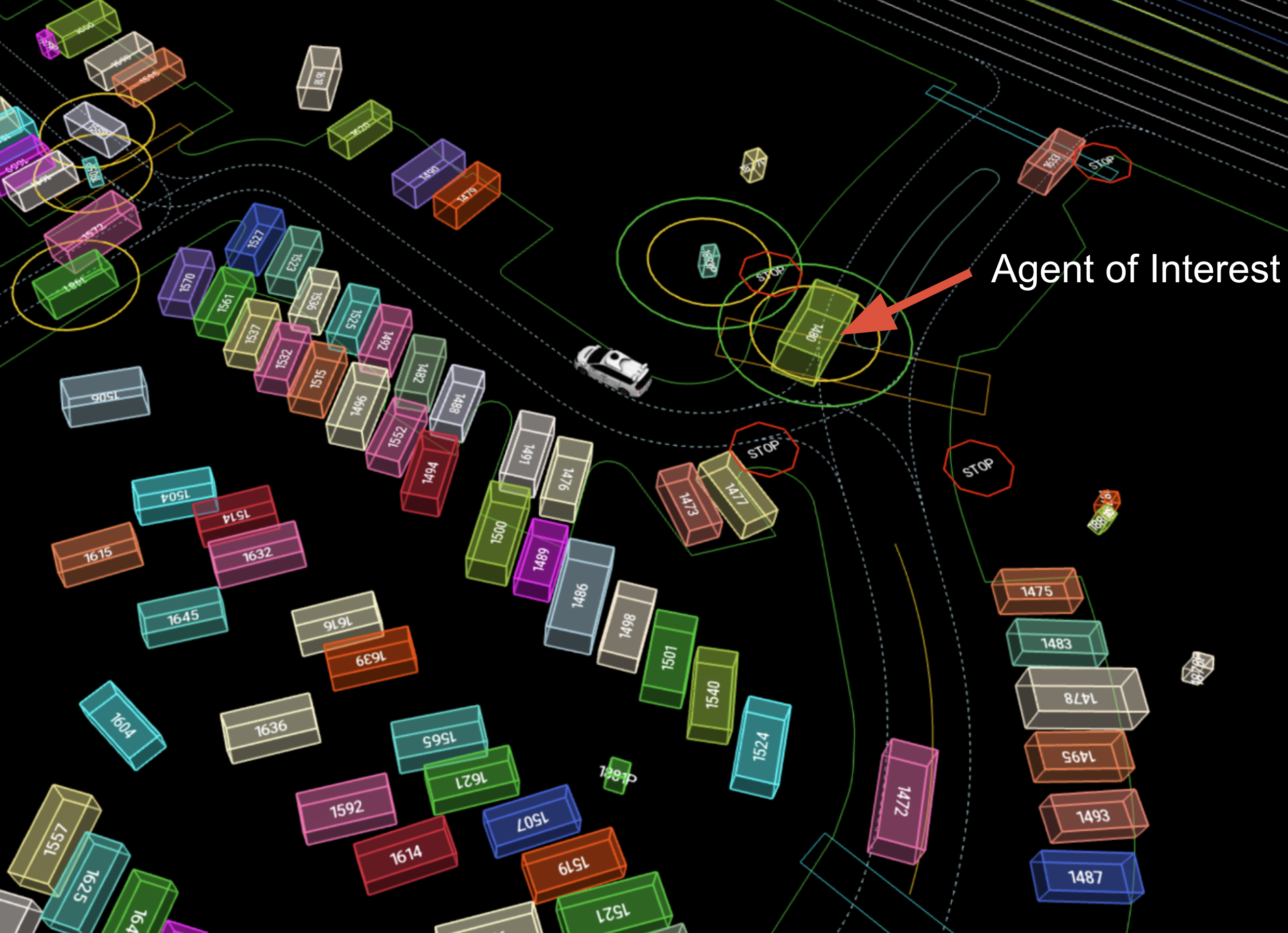
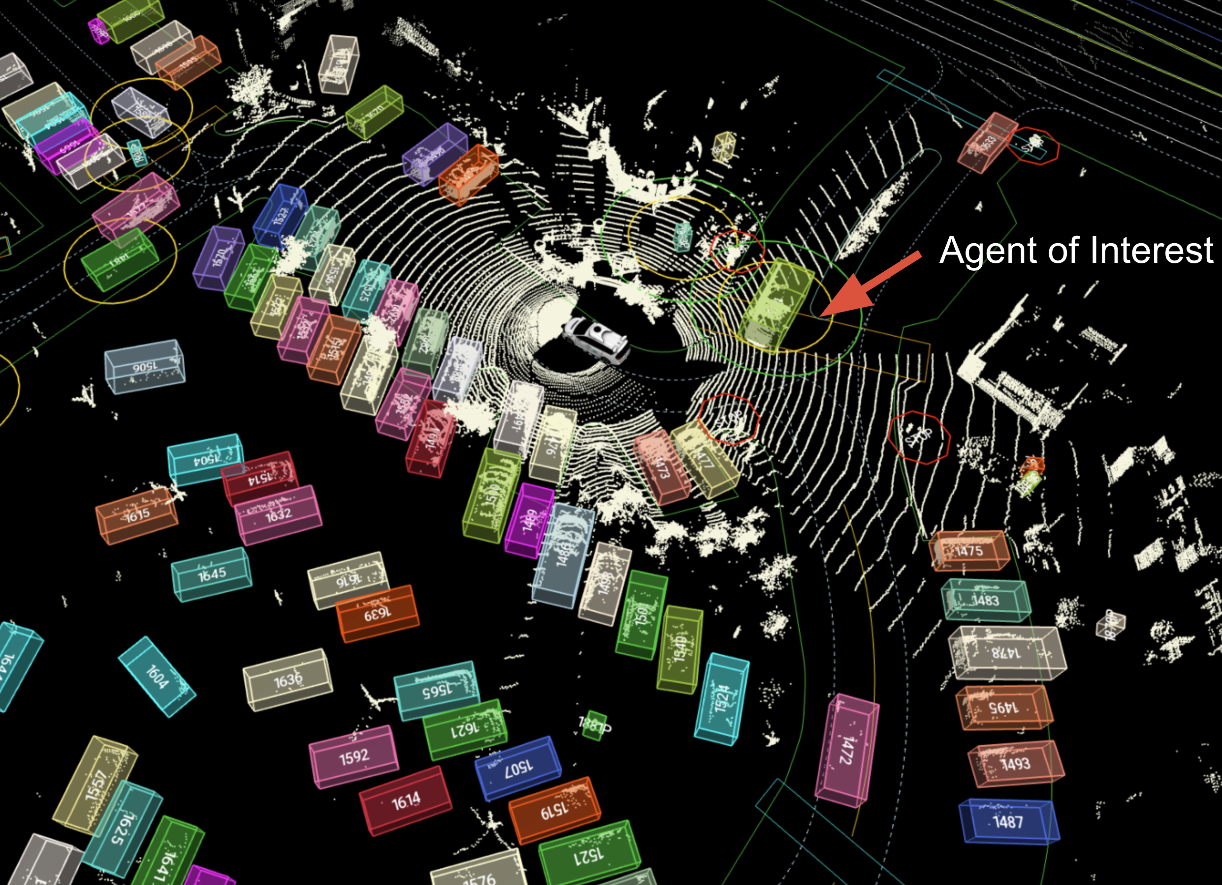
(a) A simulated scene with sophisticated interactions with (left) and without LiDAR (right).

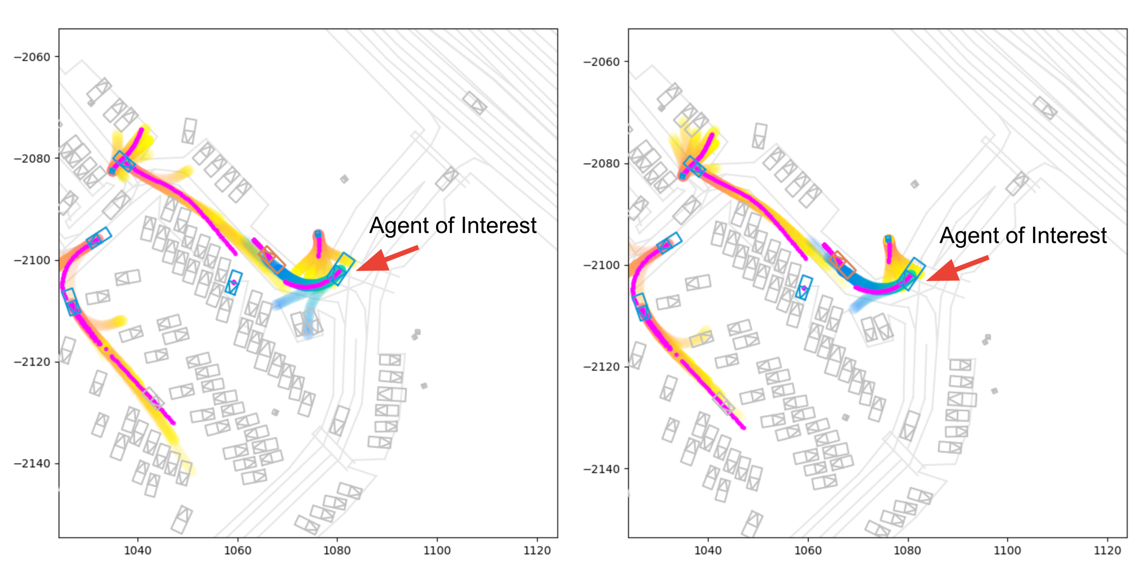
(b) Predicted trajectories with (left) and without LiDAR data (right).

Figure 1: Human-interpretable labels from the perception system provide limited information at the scene level and the object level. In sophisticated scenes with interaction between multiple objects, raw sensor data provides rich information and helps improve the motion forecasting performance. Legends in the figure: Yellow and blue (highlighted) trajectories are predictions for different agents. Red dotted lines are agents’ ground truth trajectories. Better viewed in color and zoom in for more details.

	INTERACTION	Woven Planet	Shifts	Argoverse 2	nuScenes	WOMD-LiDAR
Has LiDAR Data					✓	✓
# Segments	-	170k	600k	250k	1k	104k
Segment Duration	-	25s	10s	11s	20s	20s
Total Time	16.5h	1118h	1667h	763h	5.5h	574h
Unique Roadways	2km	10km	-	2220km	-	1750km
Sampling Rate	10Hz	10Hz	5Hz	10Hz	2Hz	10Hz
# Cities	6	1	6	6	2	6
3D Maps			✓	✓		✓
Dataset Size†	-	22GB	120GB	58GB	48GB	2.29TB*

Table 1: Comparison of the popular behavior prediction and motion forecasting datasets. We compare our WOMD-LiDAR with INTERACTION [49], Woven Planet [26], Shifts [33], Argoverse 2 [47], nuScenes [9]. “-” indicates that the data is not available or not applicable. † The sizes for other datasets are from [47]. *WOMD-LiDAR dataset size is after compression with $\sim 8\times$ compression ratio.

The absence of the raw sensor data leads to the following limitations: 1) Motion forecasting relies on lossy representation of the driving scenes (Fig. 1). The human designed interfaces lack the specificity required by the motion forecasting task. For example, the taxonomy of the agent types in Waymo Open Motion Dataset (WOMD) [17] is limited to only three types: vehicle, pedestrian, cyclist. In practice, we interact with agents who might be hard to fit into this taxonomy such as pedestrians on scooters or motor cyclists. Moreover, the fidelity of the input features is quite limited to 3D boxes that hide many important details such as pedestrian postures and gaze directions. 2) Coverage of driving scene representation is centered around where the perception system detects objects. The detection task becomes a bottleneck of transferring information to motion forecasting and planning when we are not sure if an object exist or not, especially in the first moments of an object surfacing. We hope for more graceful transmission of information between the systems that is error-robust. 3) Training perception models to match these intermediate representations might evolve them into overly complicated systems that get evaluated on subtasks that are not well correlated with overall system quality.

The goal of this work is to provide a large-scale, diverse raw sensor dataset for the motion forecasting task. We aim to augment WOMD [17] with LiDAR data in a similar format of WOD [42] for the motion forecasting task, with 100$\times$ more scenes than those available in WOD [42]. To the best of our knowledge, it is the largest publicly available LiDAR dataset across perception or motion forecasting tasks (Table 1). To overcome the huge data storage problem and make the dataset user-friendly for academic research, we adopt state-of-the-art LiDAR compression technology [51]. It reduces the LiDAR dataset by $\sim 8\times$, resulting in the final WOMD-LiDAR data to be around 2.3 TB.

To demonstrate the usefulness of the new LiDAR data, we propose a novel and simple motion forecasting baseline, which leverages raw LiDAR data to boost prediction accuracy. Instead of jointly training the perception and prediction networks, which is too demanding in memory usage, we take a two-stage approach: we first apply a perception model [43] to extract embedding features from LiDAR data. Then we feed these embeddings to a WayFormer model [35] during training. We evaluate the motion forecasting model with same metrics as WOMD [17]. Experiments show that, with LiDAR data, the WayFormer model has a 2% increase in mAP for Vehicle and Pedestrian prediction respectively. This indicates that the WOMD-LiDAR brings useful information and can further improve motion forecasting models’ performance.

The WOMD-LiDAR data has been made publicly available to the research community, and we hope it will provide new directions and opportunities in developing end-to-end motion forecasting models. Additionally, WOMD-LiDAR opens to door for potentially new research on detection and tracking with a very large amount of 3D boxes and tracks.

We summarize the contributions of our work as follows:

• We release the largest scale LiDAR dataset for motion forecasting with high quality raw sensor data across a wide spectrum of diverse scenes.

• We provide a baseline that boosts the motion forecasting performance using the raw data, demonstrating the utility of the sensor inputs.

• We design an encoding scheme that utilizes intermediate perception representations as a feature extraction utility for motion forecasting models.

2 Related Work

Motion forecasting datasets. There has been an increasing number of motion forecasting datasets [17, 26, 25, 9, 47, 49, 39, 15, 36, 30, 4, 8, 6] released. Table 1 shows the comparison for several most relevant motion forecasting datasets which aim at real-world urban driving environments. The Woven Planet prediction dataset [26] processed raw data through their perception system with over 1000 hours of logs for the traffic agents. nuScenes [9] is an autonomous driving dataset that supports detection, tracking, prediction and localization. But both of these [26, 9] did not explicitly collect or upsample diverse, complex or interactive driving scenarios. Argoverse [14, 47] mined for vehicles in various scenarios like intersections, dense traffic, etc. The INTERACTION dataset [49] collects some interactive scenarios (e.g., roundabouts, ramp merging). The Shifts [33] dataset targets vehicle motion prediction and has the longest duration. However, many of these long-duration datasets [26, 49, 33] lack LiDAR data, blocking the exploration of end-to-end motion forecasting. nuPlan [10], which is a dataset focusing on the planning of the ego vehicle, released a subset of the entire LiDAR dataset due to the vast scale. Compared with other autonomous driving perception datasets [42, 9, 19, 3] that provide LiDAR frames, our WOMD-LiDAR is significantly larger in terms of the total time, number of scenes and object interactions.

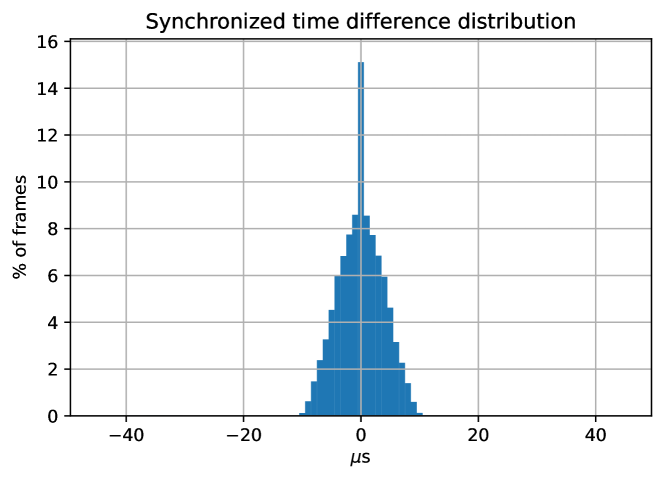
Figure 2: Synchronization difference in microseconds ($\mu$s) between LiDAR data and machine generated labels of WOMD [17]. Most time differences are within +/- 50 $\mu$s.

Motion forecasting modeling. One popular approach is to render each input frame as a rasterized top-down image where each channel represents different scene elements [13, 16, 29, 23, 12, 50]. Another method is to encode agent state history using temporal modeling techniques like RNN [34, 28, 2, 38] or temporal convolution [31]. In these two methods, relationships between each entity are aggregated through pooling [50, 48, 2, 21, 29, 34], soft attention [34, 50] and graph neural networks [11, 28, 31]. Recently, some works [35, 41] explore the Transformer [46] encoder-decoder structure for multimodal motion prediction. We choose WayFormer [35] as our motion forecasting model baseline: it is a state-of-the-art model, which can flexibly integrate features from our new LiDAR modality.

LiDAR data compression. Releasing the LiDAR data for our dataset presents a data storage challenge: without LiDAR compression techniques, the raw sensor data of WOMD-LiDAR exceeds 20 TB. As valuable as the data is, the size of it is inconvenient for fast distribution in the research community. Fortunately, in recent years, there is a growing interest in the LiDAR point cloud compression techniques. For example, one major stream of work, octree-based methods, which represent and compress quantized point clouds [7, 40], has been released as a point cloud compression standard [20]. More recently, neural network based octrees squeeze methods have been proposed, such as Octsqueeze [27], MuSCLE [5] and VoxelContextNet [37]. Alternatively, LiDAR point clouds can be stored as range images. A family of image-based compression methods have been adapted for the task. For example, traditional methods such as JPEG, PNG and TIFF have been applied to compressing range images [1, 24]. Recently, RIDDLE [51] extends such method by applying a deep neural network and delta encoding to compress range images. We adopt the delta encoder of RIDDLE [51] and reduce the raw sensor data by $\sim 8\times$.

3 Dataset

In this section, we describe the WOMD-LiDAR dataset statistics, the LiDAR data format, and the compression technique used to reduce the storage footprint.

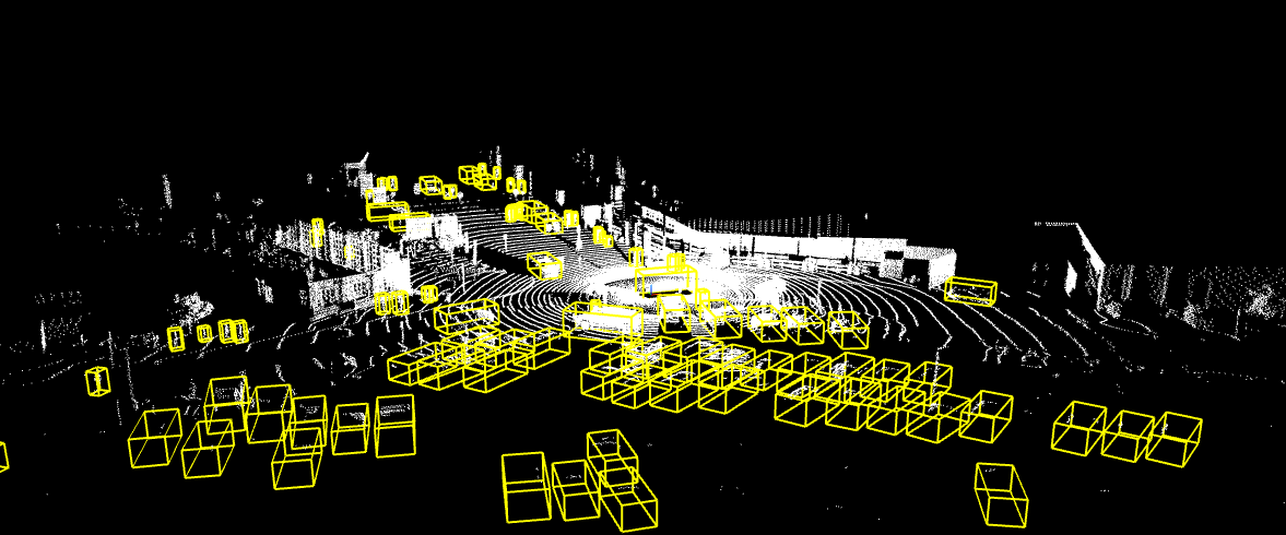
Figure 3: Visualization of LiDAR point cloud with auto-labeled boxes in one scene from WOMD-LiDAR.

Figure 4: Visualization of a range image from the top LiDAR sensor in WOMD-LiDAR. The three rows are showing range, (normalized) intensity, and (normalized) elongation from the first LiDAR return (second return omitted due to brevity). We crop the range images to only show the front 180^∘.

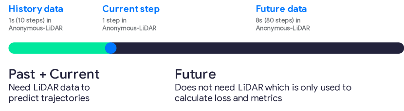
Figure 5: LiDAR data of WOMD-LiDAR in future steps is not necessary for training a motion forecasting model. The first 1 second (11 steps) contains past and current data where LiDAR is needed as input for a motion forecasting model. The rest of 8 second (80 steps) in the scene contains future steps’ data, where only ground truth is needed to calculate loss and metrics.

3.1 Dataset Statistics

To evaluate motion forecasting models on WOMD-LiDAR, we leverage existing labels gathered from WOMD [17]. The LiDAR data is highly synchronized with the machine-generated labels, with a tiny time difference due to the frame sampling during the machine label generation procedure. We calculate the difference between LiDAR data and the machine-generated label timestamps. As shown in Fig. 2, the maximum synchronization time difference is within +/- 50 microseconds, less than one time step (0.1 second at 10Hz). Fig. 3 shows an example scene with the LiDAR point cloud.

We follow the WOMD dataset format, and extract 9 second scenarios containing LiDAR data. WOMD-LiDAR is split into a 70% training, 15% validation, and 15% test set with the same run segments in WOMD. For training a motion forecasting model, it is sufficient to only use the past and current timestamps’ LiDAR data, while the future timestamps are used as ground truth to calculate loss and metrics (See Fig. 5). We only release the first 1 second LiDAR data for each scene. This helps reduce the 87.9% size of the raw LiDAR data. However, it still reaches $\sim$20TB data storage. We further apply a LiDAR compression method to reduce its size (Section 3.3).

Datasets comparison: Compared with WOD [42], one of the largest datasets for the perception task, our WOMD-LiDAR contains $100\times$ more scenes, $80\times$ total hours. nuScenes [9] is currently the only other LiDAR dataset suitable for the motion forecasting task. WOMD-LiDAR is significantly larger than nuScenes, with 104k segments ($100\times$) and 574 hours of total time ($100\times$). A more detailed comparison can be found in Table 1.

3.2 LiDAR Data Format

LiDAR data is encoded in WOMD-LiDAR as range images $\in\mathbb{R}^{h\times w\times 6}$. Following the format of WOD [42], the first two returns of LiDAR pulse are provided. Range images are collected from five LiDAR sensors. For top LiDAR, $h=64,w=2650$. For other sensors, $h=116,w=150$. Each pixel in the range images includes the following:

• Range (scalar): The distance between the origin of LiDAR sensor frame and the LiDAR point.

• Intensity (scalar): It is a measurement describing the return strength of the laser pulse that produces the LiDAR point, which is partially based on the reflectivity of the object struck by the laser pulse.

• Elongation (scalar): The elongation of the laser pulse beyond its normal width.

• Vehicle pose ($\in\mathbb{R}^{3}$): The pose of the vehicle when the LiDAR point is captured.

The range image format is necessary to exploit efficient compression schemes to reduce storage requirements (More details are provided in Section 3.3). Fig. 4 shows the different features that constitute the range images through mono-chromatic images, one for each feature. We will provide a tutorial to show how to decompress range images and convert them into the features above.

Figure 6: Model structures of LiDAR encoder (left) and motion forecasting model (right). To encode LiDAR data, we adopt a pre-trained SWFormer [43] model and extract the embedding features (which can be decoded to produce detection results). Those features (in the light yellow box) from different scales are concatenated and fed to a WayFormer [35] model as a new modality feature for the motion forecasting task. Better viewed in color and zoom in for more details.

3.3 LiDAR Data Compression

Storing raw sensory data is prohibitively expensive. Therefore, we apply the delta encoding compressor proposed in [51]. We use a non-deep-learning version of the algorithm for fast compression and decompression. This compression is lossless under a pre-specified quantization precision. Therefore, we do not expect to impact the goals of end-to-end learning research agenda.

The basic idea of the algorithm is to use a previous pixel value in the range image to predict the next valid pixel (the closest valid one on its right in the spatial domain) value. Therefore, instead of storing the absolute pixel values, we store the residuals between the predictions and the original pixel values. Since the residuals have a more concentrated distribution (especially on quantized range images) with lower entropy, they are compressed to a much smaller size with varint coding followed by zlib compression.

In our implementation, we quantize the range image channels with the following precision: range 0.005m, intensity 0.01m , elongation 0.01m, pose translation 0.0001m, pose rotation 0.001 radians. We leverage the default varint coding from the publicly available Google Protobuf implementation (for uint and bool fields). We will release our compression algorithm together with the dataset.

4 Motion Forecasting Model with LiDAR

To validate the effectiveness of WOMD-LiDAR, we train a WayFormer [35] model using LiDAR embeddings as a baseline. We describe the details of the motion forecasting model and the LiDAR encoder (Fig. 6) in this section.

4.1 Motion Forecasting Model

We choose WayFormer [35] as the motion forecasting baseline model and the backbone for any extensions. It adopts a transformer based scene encoder which is flexible to plug in features from various modalities. We extend the original WayFormer model which fuses features from agent history states, traffic light signals, agent interaction states and road graph features, by adding additional LiDAR modality fed to the scene encoder. The features of LiDAR modality are generated from a SWFormer extractor and a LiDAR encoder. During the training, we freeze the gradients of the SWFormer feature extractor and update only the LiDAR encoder’s model parameters. After applying the scene encoder to fuse multi-modal features, the output embeddings are fed to the trajectory decoder to produce the final predicted trajectories.

4.2 LiDAR Encoding Scheme

We adopt a pre-trained SWFormer [43] to extract LiDAR embeddings. The SWFormer is trained on WOD [42] for the 3D object detection task. The SWFormer adopts sparse partition operators and transformer based layers to encode LiDAR data from different scales. We extract the embedding features which are used to produce detection results in the detection heads as the input to the scene encoder of WayFormer model. These features effectively encode rich information of objects and context environment from noisy LiDAR points. To provide context agent information, we lower the detection confidence threshold to produce more but less reliable detected objects. This increases the recall of the detection results but decreases the precision. In addition to the embedding features, we also pad more features:

• Detected box coordinates: We append the detected boxes center coordinates to emphasize the potential detected objects positions.

• Detected box size: The height, width, length of the boxes provide useful hints of objects from different categories.

• Foreground probability from the segmentation head: This helps reduce the noise from detection results.

The output tensor $E$ from SWFormer with padded features is a $N\times T\times C$ tensor, where $N$ is the number of detected boxes, $T$ is the number of input frames, $C$ is the feature size. To adapt $E$ to be compatible as input for the scene encoder of WayFormer, we flatten the first two dimensions as the token dimension. A one-layer Axial Transformer [22] is applied as a LiDAR encoder to project the output tensor $E$ to be a fixed $M$-token tensor $E^{\prime}\in\mathbb{R}^{M\times C^{\prime}}$ with the same feature size as other modalities.

5 Experiments

The WayFormer model is evaluated on the standard motion forecasting task on WOMD-LiDAR.

Set	Model	Vehicle			Pedestrian			Cyclist
		minADE $\downarrow$	MR $\downarrow$	mAP $\uparrow$	minADE $\downarrow$	MR $\downarrow$	mAP $\uparrow$	minADE $\downarrow$	MR $\downarrow$	mAP $\uparrow$
	LSTM [17]	1.34	0.25	0.23	0.63	0.13	0.23	1.26	0.29	0.21
Standard Validation	Wayformer [35]	1.10	0.18	0.35	0.54	0.11	0.35	1.08	0.22	0.29
	Wayformer + LiDAR	1.09	0.17	0.37	0.54	0.10	0.37	1.06	0.21	0.28

Table 2: Marginal metrics on the standard validation set. All metrics computed at 8s. We compare WOMD [17] baseline, WayFormer [35] and WayFormer trained with LiDAR data on the WOMD-LiDAR standard motion forecasting track.

5.1 Experiment Setup

LiDAR Feature Extractor. We train the SWFormer [43] on WOD [42] as the LiDAR feature extractor. We set batch size as 4, training 80,000 steps on 64 V3 TPUs. The IOU thresholds for vehicles and pedestrians are 0.7 and 0.5 respectively. In the original SWFormer inference stage, the boxes are filtered if the predicted confidence is less than 0.5. To extract feature embeddings, we need more context information and high recall of the detection results. Thus, we lower the box confidence threshold $\tau$ to be 0.1 (see ablation study in Section 5.4). The extracted embeddings are 128D vectors. With box coordinates ($x$, $y$, $z$), box size (width, length, height) and foreground probability, the final LiDAR features are 135D vectors ($C=135$) fed to the scene encoder of the WayFormer [35]. We set the maximum number of detected boxes in each frame as 140 ($N\leq 140)$. If there are more than 140 detected objects, we discard the detected objects with low box confidence scores. We set the number of output tokens of the LiDAR encoder as $M=10$ before sending the embeddings to the scene encoder.

Motion Forecasting Model. We follow WayFormer [35] settings on WOMD and use a batch size of 16. The WayFormer model is trained with 1.2M steps on 16 V3 TPUs. We project all modalities to the same feature size of 256D ($C^{\prime}=256$), then utilize cross-attention with latent queries to reduce the number of tokens to 192. The scene encoder has 2 transformer layers. WayFormer encodes the history states of 1 second (10 steps at 10Hz) and predicts K=6 trajectories for each agent’s future 8 seconds.

5.2 Metrics

We use the WOMD motion forecasing challenge metrics [17]. Given an input sample, a motion forecasting model predicts $K$ possible trajectories for $N$ agents in the scene for the future $T$ steps $\mathbf{x}^{k}=\{x_{i,t}\}_{i=1:N,t=1:T}$. We denote the corresponding ground truth trajectories as $\mathbf{y}=\{y_{i,t}\}_{i=1:N,t=1:T}$.

minADE. The minimum Average Displacement Error calculates the $\ell_{2}$ distance between the predicted trajectory which is closest to the ground truth across all time steps:

$$\text{minADE}=\min_{k}\frac{1}{NT}\sum_{i}\sum_{t}||\mathbf{x}^{k}_{i,t}-\mathbf{y}_{i,t}||_{2}$$ (1)

Miss Rate (MR). MR measures whether the closest predicted trajectory $\min_{k}\mathbf{x}^{k}_{i,t}$ matches the ground truth $\mathbf{y}_{i,t}$. The MR at time step $t$ is calculated as:

$$\text{MR}_{t}=\min_{k}\vee_{i}\neg\texttt{IsMatch}(\mathbf{x}^{k}_{i,t},\mathbf{y}_{i,t})$$ (2)

More details of the function IsMatch implementation can be found in the WOMD dataset [17].

Mean Average Precision (mAP). mAP is similar to the one for object detection task [32]. It computes precision-recall curve’s integral area by varying confidence threshold for the predicted trajectories. The criteria of judging whether a trajectory is a true positive, false positive, etc. is consistent with the MR definition in Eq. 2. For each object, only the trajectory with the highest confidence is used to calculate the mAP for the corresponding true positive.

5.3 Baseline Model Performance

We evaluate our baseline model on the WOMD-LiDAR validation set. The results are shown in Table 2. With LiDAR features, our model performs better than WayFormer for vehicle, pedestrians and cyclists on the Missing Rate (MR) metric, with 0.01 decrease in each category respectively. This indicates LiDAR information provides location hints for WayFormer. For minADE metrics, the results are roughly the same. WayFormer with LiDAR inputs also achieves 2% increase in mAP for vehicle and pedestrian categories. This is because LiDAR features provide more information about the object locations, shapes and interactions with other objects. They help the WayFormer model understand the scene and predict more accurate trajectories. For cyclists, there is a minor regression in mAP. It is likely due to the fact that the LiDAR points are noisy in this category and we may need a better encoding method to extract useful information.

5.4 Ablation Study

We conduct an ablation study of our baseline model on WOMD-LiDAR. In the following experiments, we report the average minADE, MR and mAP across vehicle, pedestrian and cyclist categories at 3s, 5s and 8s on the WOMD-LiDAR validation set.

Threshold of SWFormer to extract embeddings. As described in Sec. 5.1, we lower the SWFormer threshold $\tau$ to get high recall of detected boxes so that we could get more context information in the scene. We sweep the threshold of SWFormer from 0.0 to 0.5 (default value of SWFormer), and generate different training datasets extracted from WOMD-LiDAR and evaluate the corresponding performance of the baseline model. When the threshold $\tau$ is lower, the number of predicted boxes from SWFormer becomes larger. This brings more context information for motion forecasting model while it also brings more noise in the inputs. As shown in Table 3, the WayFormer’s performance is not so sensitive to $\tau$. When $\tau=0.1$, the WayFormer with LiDAR inputs achieves the best performance. When $\tau$ further increases, the number of detected boxes becomes smaller and may result in loss of useful information.

Threshold $\tau$	minADE $\downarrow$	MR $\downarrow$	mAP $\uparrow$
0.0	0.5692	0.1401	0.4005
0.1	0.5553	0.1292	0.4191
0.3	0.5623	0.1399	0.4102
0.5	0.5675	0.1410	0.4087

Table 3: Experiment results of sweeping SWFormer threshold $\tau$ to extract embeddings. The metrics are evaluated on WOMD-LiDAR validation set, averaged across categories, and over results at 3s, 5s, and 8s.

Model	minADE $\downarrow$	MR $\downarrow$	mAP $\uparrow$
No boxes coordinates	0.5852	0.1594	0.3947
No boxes sizes	0.5773	0.1476	0.4008
No foreground prob.	0.5601	0.1331	0.4110
Wayformer with LiDAR	0.5553	0.1292	0.4191

Table 4: Experiment results of masking out additional features in LiDAR encoding (Sec. 4.2). The metrics are evaluated on WOMD-LiDAR validation set), averaged across categories, and over results at 3s, 5s, and 8s.

Different embedding features. There are three additional features (Sec. 4.2) included in the embedding output from the LiDAR encoder: detected box coordinates, size and foreground probability. We mask out each feature and check the WayFormer model performance in Table 4. The experiments show that without box coordinates, the minADE, MR, mAP regress by 0.0299, 0.0302, 0.0244 respectively. This indicates that aside from the SWFormer embedding features, the box coordinates play an important role in motion forecasting . Compared to masking out box coordinates, masking out box sizes has a smaller regression, with minADE, MR increased by 0.022 and 0.0184 and mAP decreased by 0.0183. Foreground probability also contributes slightly to the overall performance, with regression in the minADE, MR, mAP as 0.0048, 0.0039, 0.0081 respectively.

# tokens of embeddings	minADE $\downarrow$	MR $\downarrow$	mAP $\uparrow$
16	0.6011	0.1702	0.3811
32	0.5888	0.1610	0.3907
64	0.5797	0.1503	0.3998
192	0.5553	0.1292	0.4191
# layers of transformer	minADE $\downarrow$	MR $\downarrow$	mAP $\uparrow$
1	0.5711	0.1440	0.3991
2	0.5553	0.1292	0.4191
3	0.5561	0.1325	0.4112

Table 5: Experiment results of scene encoder’s #tokens and #transformer layers. The metrics are evaluated on WOMD-LiDAR validation set, averaged across categories, and over results at 3s, 5s, and 8s.

WayFormer modeling. We study the WayFormer hyper-parameters in motion forecasting. Specifically, we conduct experiments to investigate the impact of number of tokens and layers of the scene encoder. This is because the scene encoder provides encoded embeddings for the trajectory decoder in the prediction stage. The embedding quality plays an important role for the motion forecasting task. As shown in Table 5, the number of embedding tokens impacts quality more than the number of scene encoder transformer layers. When we increase the token size from 16 to 192 (the default WayFormer setting), the minADE and MR decrease from 0.6011 to 0.5553 and 0.1702 to 0.1292, respectively, and mAP increases from 0.3811 to 0.4191. This indicates that when the token size increases, more information will be encoded in the embeddings for motion prediction.

We also vary the number of transformer blocks from 1 to 3 (Table 5). The performance of WayFormer model first improves (# layers increases from 1 to 2) and then regresses (# layers increases from 2 to 3). Thus, we set the optimal value of # layers of the scene encoder as 2.

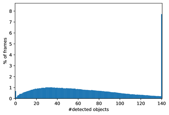
Figure 7: Distribution of the number of detected objects by SWFormer in each frame of WOMD-LiDAR.

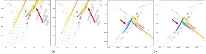
Figure 8: Visualization of prediction result comparison between WayFormer [35] (sub-figures on the left) and WayFormer with LiDAR inputs (sub-figures on the right). Fig (a): With LiDAR information the predicted trajectories avoid crashing into parked cars. Fig (b): The predicted trajectories of cyclists avoid crashing into cars. Legends in the figure: Yellow and blue trajectories are predictions for different agents, while blue trajectories are highlighted ones. Red dotted lines are labeled ground truth trajectories for agents in the scene. Better viewed in color and zoom in for more details.

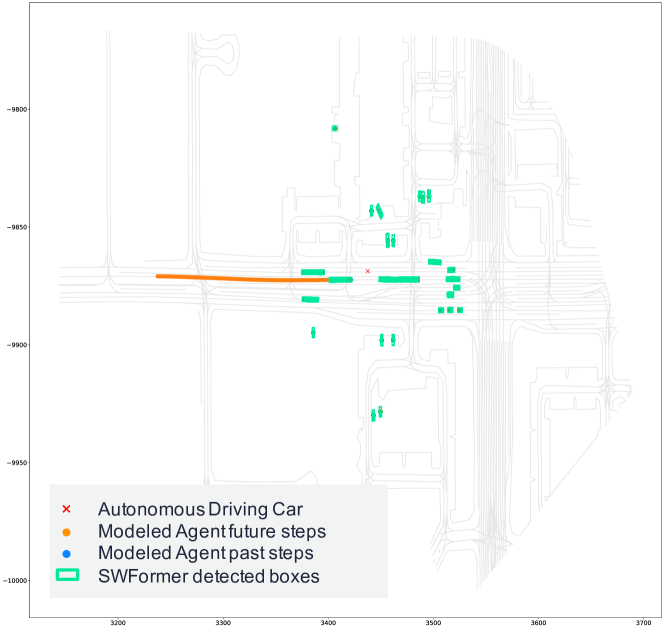
Figure 9: Visualization of SWFormer detection results on one of WOMD-LiDAR scenes. The detected boxes of different objects form continuous trajectories across different time steps.

5.5 Qualitative Results

We visualize the SWFormer detection results and the WayFormer prediction results on WOMD-LiDAR to check the quality of detection and motion forecasting.

Distribution of detected objects per frame. We visualize the distribution of the number of objects detected by SWFormer. As shown in the Fig. 7, the average number of detected objects is 65.13. SWFormer detects all frames with the maximum threshold of objects (140), which provides rich context information for motion forecasting.

Visualization of WayFormer prediction results. We visualize some prediction results and conduct analysis on the prediction quality. As shown in Fig. 8, with LiDAR inputs, WayFormer model avoids collision into vehicles, pedestrians and cyclists. Specifically, in Fig 8(a), with LiDAR information, the predicted trajectories avoid crashing into parked cars. In Fig 8(b), the predicted trajectories of cyclists avoid crashing into cars. We observe more reasonable predicted trajectories, matching the improved performance in Table 2. More visualization results are available in the supplementary material.

Visualization of SWFormer detection results. To verify the SWFormer extracted meaningful embeddings, we need to confirm the detection results on WOMD-LiDAR. As shown in Fig. 9, we decode the embeddings and visualize SWFormer’s detection results for the first 11 time steps for different agents, including the vehicles, pedestrians and cyclists. Detection results show that SWFormer successfully detects objects in different time steps and these detection results formulate continuous trajectories.

6 Conclusion and Future Directions

Conclusion. In this work, we augment WOMD with the largest scale LiDAR dataset in the community, containing LiDAR point clouds for more than 100,000 scenes. To resolve the huge data storage requirements, we adopt state-of-the-art LiDAR data compression technology and successfully reduce the dataset size to be less than 2.5 TB. To evaluate the suitability of LiDAR to the motion forecasting task, we provide a WayFormer baseline trained with LiDAR. Experiments show that LiDAR data brings improvement in the motion forecasting task. We hope WOMD-LiDAR could provide great opportunities for further advancing end-to-end motion forecasting research.

Limitations and future work. 1) In this work, we only trained WayFormer and WayFormer + LiDAR models. We will investigate end-to-end models that can directly encode LiDAR point clouds with motion forecasting task in mind. 2) The SWFormer detector, which serves as the point cloud encoder in our model, can only represents object-level information. We will look into some approaches that can leverage scene-level information, that are not sensitive to the detection prediction thresholds. 3) Another interesting direction is to explore methods that solely depends on the sensor data to avoid the reliance on the human-defined sparse objects as an interface.

Acknowledgement. We thank Alexander Gorban and Ben Sapp for their insightful comments, and the Waymo Research team members for their support.

Appendix A Supplementary Dataset Details

	INTERACTION	Woven Planet	Shifts	Argoverse 2	nuScenes	WOMD-LiDAR
Offboard Perception	✓					✓
Mined for Interestingness	-	-	-	✓	-	✓
Traffic Signal States		✓	✓			✓

Table 6: Comparison of the popular behavior prediction and motion forecasting datasets. “-” indicates that the data is not available or not applicable. “Offboard perception” is checked if the labels were auto-labeled by offboard perception which can generate high-quality labels. “Mined for Interestingness” is checked if the dataset mined interesting interactions after the data collection. “Traffic Signal States” is checked if the dataset provided traffic light states.

# output tokens ($M$)	minADE $\downarrow$	MR $\downarrow$	mAP $\uparrow$	# layers	minADE $\downarrow$	MR $\downarrow$	mAP $\uparrow$
5	0.5700	0.1501	0.3999	1	0.5553	0.1292	0.4191
10	0.5553	0.1292	0.4191	2	0.5613	0.1392	0.3998
20	0.5594	0.1313	0.4102	3	0.5610	0.1398	0.4001

Table 7: Experiment results of the number of output tokens $M$ and the number of transformer layers in the LiDAR encoder. The metrics are evaluated on WOMD-LiDAR validation set, averaged across categories, and over results at 3s, 5s, and 8s.

Dataset comparison. We provide more details of the dataset comparison in Table 6. In Table 1 of the main paper, “Sampling Rate” is the data collection rate in Hz. “3D Maps” indicates whether the dataset provided the 3D Map information. “Dataset Size” entries were collected by Argoverse 2 [47]. Combining Table 6 and Table 1 of the main paper, we provide the complete comparison between our WOMD-LiDAR and other datasets.

Supplementary Details of WOMD-LiDAR. Map data is encoded as a set of polylines and polygons created from curves sampled at a resolution of 0.5 meters following [17, 18]. Traffic signal states is also provided along with other static map feature types (e.g. lane boundary lines, road edges and stop signs). We followed [17] to mine the interesting scenarios in our WOMD-LiDAR.

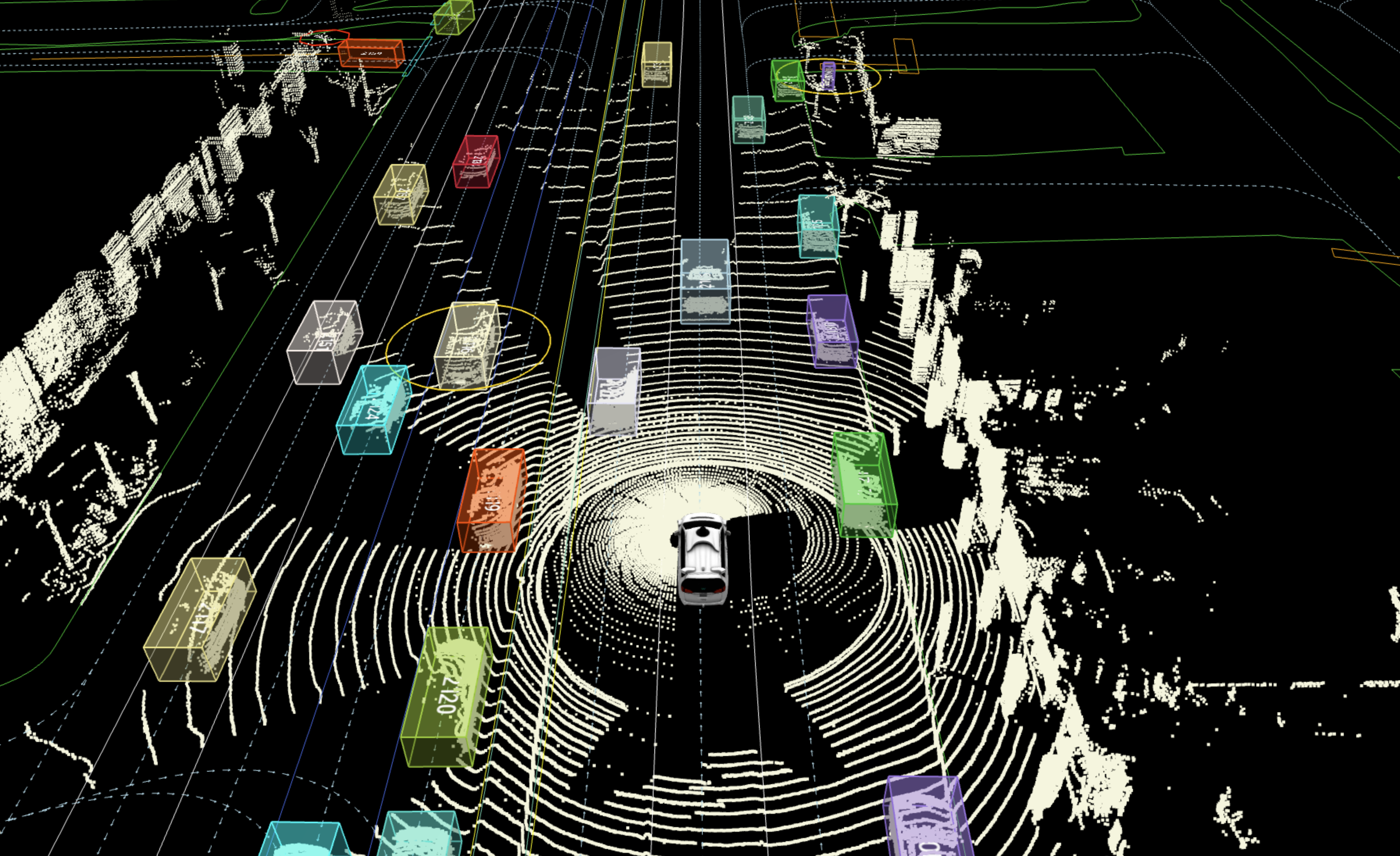
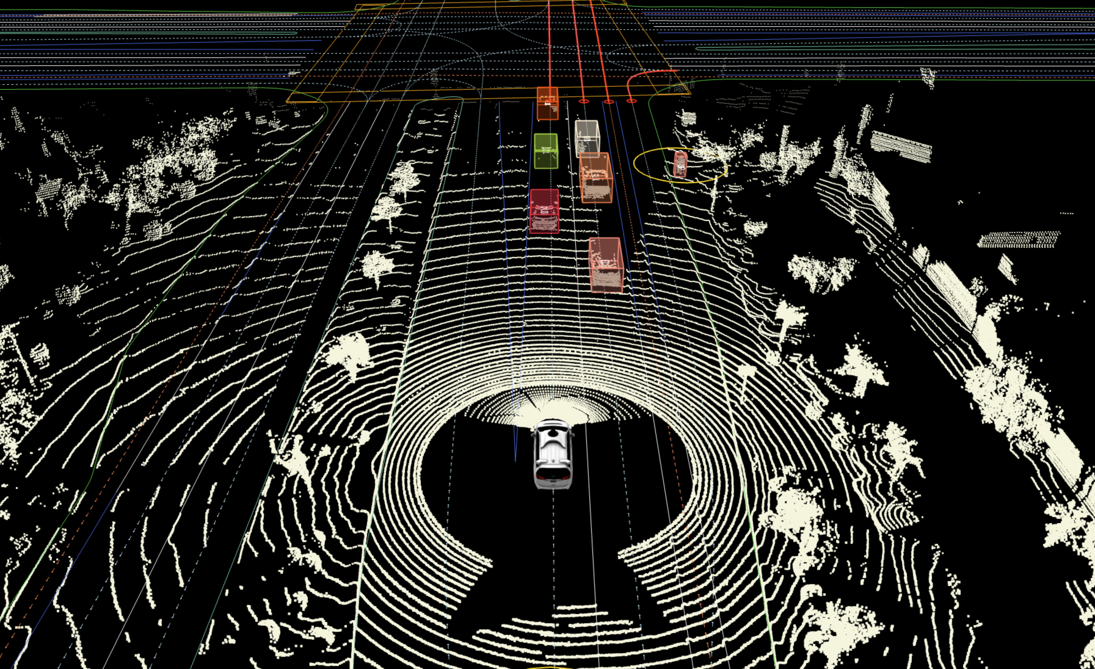
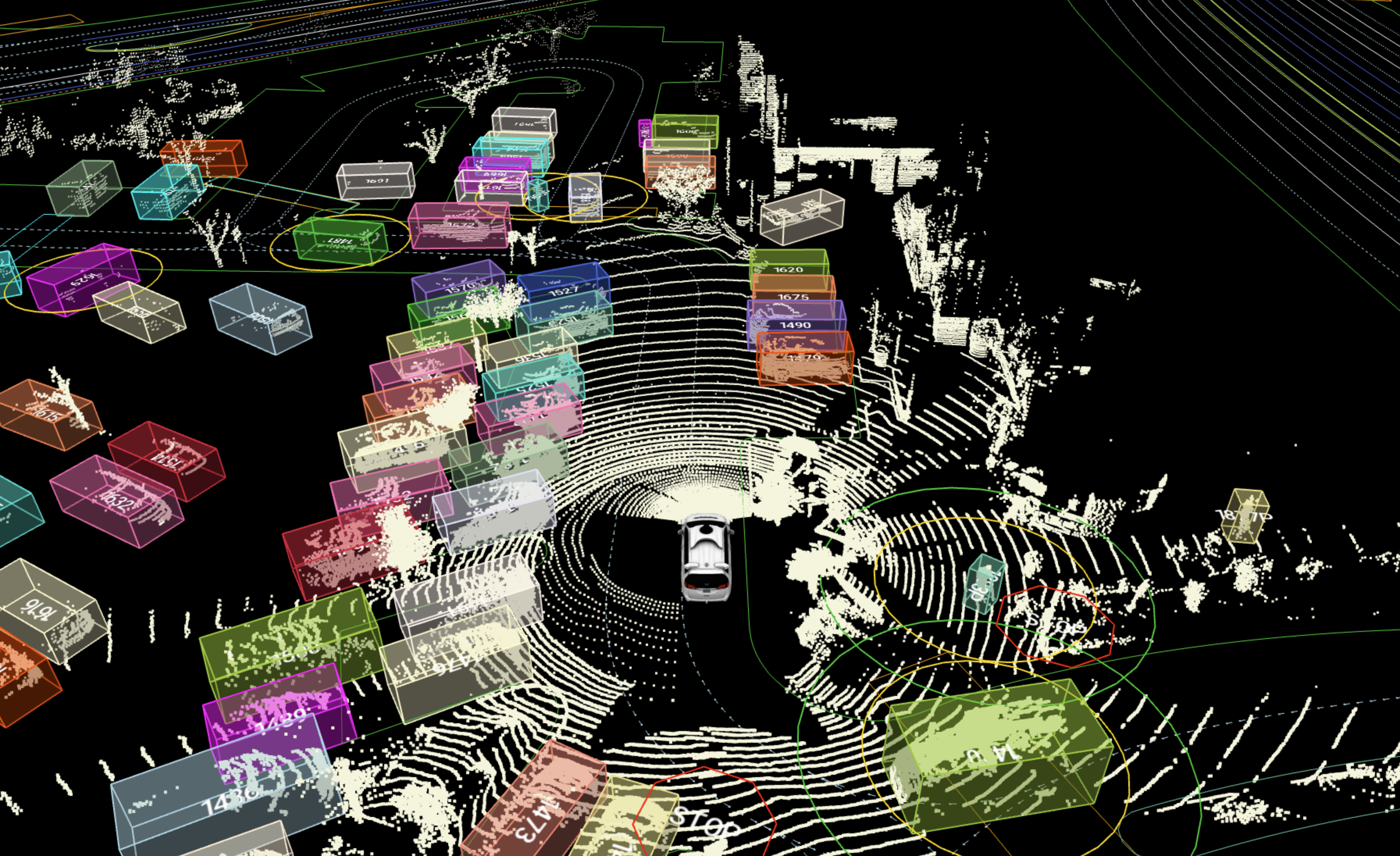
Figure 10: Scenario visualizations with LiDAR. Better viewed in color and zoom in for more details.

Appendix B Visualization

Scenario Videos with LiDAR. In Fig. 10, we provide more visualization of scenarios with not only the bounding boxes of the agents of interest, but also the released high quality well calibrated LiDAR data.

We provide some simulated scenes with both LiDAR and labeled boxes on WOMD-LiDAR. They are formulated as mov files in the supplementary materials. Each video clip contains 11 frames in slow motion, with LiDAR data visualized with the boxes of agents. This is because we only release the first 11 frames’ LiDAR data in WOMD-LiDAR.

WayFormer + LiDAR prediction visualization. We provide more visualization results in Fig. 11. From the visualization results, our WayFormer [35] + LiDAR model tries to avoid collision into other agents (vehicles, pedestrians and cyclists) in the motion forecasting task. This is consistent with the improved performance in Table 2.

Appendix C Experiments

Ablation Study of LiDAR Encoder. We provide the ablation study of LiDAR Encoder described in Section 4.2 in the submission. Specifically, we study the number of output tokens $M$ and the number of transformer layers. Experiment results are shown in the Table 7.

From the Table 7, we find when $M$ increases, the final performance of WayFormer first increases and then decreases. We set the optimal value of $M$ as 10 in our experiments. On the other side, LiDAR encoder is not so sensitive to the number of transformer layers. There is a slight regression when the number of layers increases. To achieve best performance and fast training speed, we set the number of layers as 1 in our experiments.

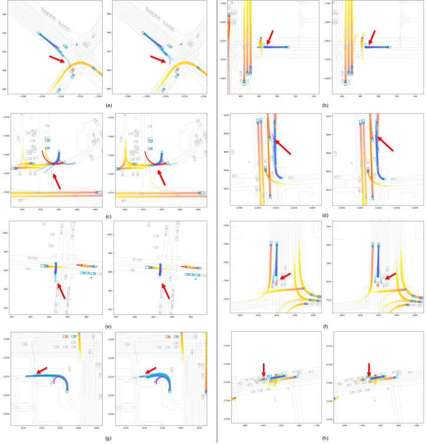
Figure 11: Visualization of prediction result comparison between WayFormer [35] (sub-figures on the left) and WayFormer with LiDAR inputs (sub-figures on the right). Legends in the figure: Yellow and blue trajectories are predictions for different agents, while blue trajectories are highlighted ones. Red dotted lines are labeled ground truth trajectories for agents in the scene. More visualization results are available in the supplementary material. Better viewed in color and zoom in for more details.

References

- [1] Jae-Kyun Ahn, Kyu-Yul Lee, Jae-Young Sim, and Chang-Su Kim. Large-scale 3d point cloud compression using adaptive radial distance prediction in hybrid coordinate domains. IEEE Journal of Selected Topics in Signal Processing, 2014.
- [2] Alexandre Alahi, Kratarth Goel, Vignesh Ramanathan, Alexandre Robicquet, Li Fei-Fei, and Silvio Savarese. Social lstm: Human trajectory prediction in crowded spaces. In CVPR, 2016.
- [3] Jens Behley, Martin Garbade, Andres Milioto, Jan Quenzel, Sven Behnke, Cyrill Stachniss, and Jurgen Gall. Semantickitti: A dataset for semantic scene understanding of lidar sequences. In ICCV, 2019.
- [4] Ben Benfold and Ian Reid. Stable multi-target tracking in real-time surveillance video. In CVPR, 2011.
- [5] Sourav Biswas, Jerry Liu, Kelvin Wong, Shenlong Wang, and Raquel Urtasun. Muscle: Multi sweep compression of lidar using deep entropy models. NeurIPS, 2020.
- [6] Julian Bock, Robert Krajewski, Tobias Moers, Steffen Runde, Lennart Vater, and Lutz Eckstein. The ind dataset: A drone dataset of naturalistic road user trajectories at german intersections. In Intelligent Vehicles Symposium (IV), 2020.
- [7] Mario Botsch, Andreas Wiratanaya, and Leif Kobbelt. Efficient high quality rendering of point sampled geometry. Rendering Techniques, 2002.
- [8] Antonia Breuer, Jan-Aike Termöhlen, Silviu Homoceanu, and Tim Fingscheidt. opendd: A large-scale roundabout drone dataset. In International Conference on Intelligent Transportation Systems (ITSC), 2020.
- [9] Holger Caesar, Varun Bankiti, Alex H Lang, Sourabh Vora, Venice Erin Liong, Qiang Xu, Anush Krishnan, Yu Pan, Giancarlo Baldan, and Oscar Beijbom. nuscenes: A multimodal dataset for autonomous driving. In CVPR, 2020.
- [10] Holger Caesar, Juraj Kabzan, Kok Seang Tan, Whye Kit Fong, Eric Wolff, Alex Lang, Luke Fletcher, Oscar Beijbom, and Sammy Omari. nuplan: A closed-loop ml-based planning benchmark for autonomous vehicles. arXiv preprint arXiv:2106.11810, 2021.
- [11] Sergio Casas, Cole Gulino, Renjie Liao, and Raquel Urtasun. Spagnn: Spatially-aware graph neural networks for relational behavior forecasting from sensor data. In ICRA, 2020.
- [12] Sergio Casas, Wenjie Luo, and Raquel Urtasun. Intentnet: Learning to predict intention from raw sensor data. In CoRL, 2018.
- [13] Yuning Chai, Benjamin Sapp, Mayank Bansal, and Dragomir Anguelov. Multipath: Multiple probabilistic anchor trajectory hypotheses for behavior prediction. CoRL, 2019.
- [14] Ming-Fang Chang, John Lambert, Patsorn Sangkloy, Jagjeet Singh, Slawomir Bak, Andrew Hartnett, De Wang, Peter Carr, Simon Lucey, Deva Ramanan, et al. Argoverse: 3d tracking and forecasting with rich maps. In CVPR, 2019.
- [15] Benjamin Coifman and Lizhe Li. A critical evaluation of the next generation simulation (ngsim) vehicle trajectory dataset. Transportation Research Part B: Methodological, 2017.
- [16] Henggang Cui, Vladan Radosavljevic, Fang-Chieh Chou, Tsung-Han Lin, Thi Nguyen, Tzu-Kuo Huang, Jeff Schneider, and Nemanja Djuric. Multimodal trajectory predictions for autonomous driving using deep convolutional networks. In ICRA, 2019.
- [17] Scott Ettinger, Shuyang Cheng, Benjamin Caine, Chenxi Liu, Hang Zhao, Sabeek Pradhan, Yuning Chai, Ben Sapp, Charles R Qi, Yin Zhou, et al. Large scale interactive motion forecasting for autonomous driving: The waymo open motion dataset. In ICCV, 2021.
- [18] Jiyang Gao, Chen Sun, Hang Zhao, Yi Shen, Dragomir Anguelov, Congcong Li, and Cordelia Schmid. Vectornet: Encoding hd maps and agent dynamics from vectorized representation. In CVPR, 2020.
- [19] Andreas Geiger, Philip Lenz, Christoph Stiller, and Raquel Urtasun. Vision meets robotics: The kitti dataset. The International Journal of Robotics Research, 32(11):1231–1237, 2013.
- [20] D Graziosi, O Nakagami, S Kuma, A Zaghetto, T Suzuki, and A Tabatabai. An overview of ongoing point cloud compression standardization activities: Video-based (v-pcc) and geometry-based (g-pcc). APSIPA Transactions on Signal and Information Processing, 2020.
- [21] Agrim Gupta, Justin Johnson, Li Fei-Fei, Silvio Savarese, and Alexandre Alahi. Social gan: Socially acceptable trajectories with generative adversarial networks. In CVPR, 2018.
- [22] Jonathan Ho, Nal Kalchbrenner, Dirk Weissenborn, and Tim Salimans. Axial attention in multidimensional transformers. arXiv preprint arXiv:1912.12180, 2019.
- [23] Joey Hong, Benjamin Sapp, and James Philbin. Rules of the road: Predicting driving behavior with a convolutional model of semantic interactions. In CVPR, 2019.
- [24] Hamidreza Houshiar and Andreas Nüchter. 3d point cloud compression using conventional image compression for efficient data transmission. In International Conference on Information, Communication and Automation Technologies (ICAT), 2015.
- [25] John Houston, Guido Zuidhof, Luca Bergamini, Yawei Ye, Long Chen, Ashesh Jain, Sammy Omari, Vladimir Iglovikov, and Peter Ondruska. One thousand and one hours: Self-driving motion prediction dataset. In CoRL, 2021.
- [26] John Houston, Guido Zuidhof, Luca Bergamini, Yawei Ye, Ashesh Jain, Sammy Omari, Vladimir Iglovikov, and Peter Ondruska. One thousand and one hours: Self-driving motion prediction dataset. https://www.woven-planet.global/en/data/prediction-dataset, 2020.
- [27] Lila Huang, Shenlong Wang, Kelvin Wong, Jerry Liu, and Raquel Urtasun. Octsqueeze: Octree-structured entropy model for lidar compression. In CVPR, 2020.
- [28] Siddhesh Khandelwal, William Qi, Jagjeet Singh, Andrew Hartnett, and Deva Ramanan. What-if motion prediction for autonomous driving. arXiv preprint arXiv:2008.10587, 2020.
- [29] Namhoon Lee, Wongun Choi, Paul Vernaza, Christopher B Choy, Philip HS Torr, and Manmohan Chandraker. Desire: Distant future prediction in dynamic scenes with interacting agents. In CVPR, 2017.
- [30] Alon Lerner, Yiorgos Chrysanthou, and Dani Lischinski. Crowds by example. In Computer graphics forum. Wiley Online Library, 2007.
- [31] Ming Liang, Bin Yang, Rui Hu, Yun Chen, Renjie Liao, Song Feng, and Raquel Urtasun. Learning lane graph representations for motion forecasting. In ECCV, 2020.
- [32] Tsung-Yi Lin, Michael Maire, Serge Belongie, James Hays, Pietro Perona, Deva Ramanan, Piotr Dollár, and C Lawrence Zitnick. Microsoft coco: Common objects in context. In ECCV, 2014.
- [33] Andrey Malinin, Neil Band, German Chesnokov, Yarin Gal, Mark JF Gales, Alexey Noskov, Andrey Ploskonosov, Liudmila Prokhorenkova, Ivan Provilkov, Vatsal Raina, et al. Shifts: A dataset of real distributional shift across multiple large-scale tasks. arXiv preprint arXiv:2107.07455, 2021.
- [34] Jean Mercat, Thomas Gilles, Nicole El Zoghby, Guillaume Sandou, Dominique Beauvois, and Guillermo Pita Gil. Multi-head attention for multi-modal joint vehicle motion forecasting. In ICRA, 2020.
- [35] Nigamaa Nayakanti, Rami Al-Rfou, Aurick Zhou, Kratarth Goel, Khaled S Refaat, and Benjamin Sapp. Wayformer: Motion forecasting via simple & efficient attention networks. arXiv preprint arXiv:2207.05844, 2022.
- [36] Stefano Pellegrini, Andreas Ess, Konrad Schindler, and Luc Van Gool. You’ll never walk alone: Modeling social behavior for multi-target tracking. In ICCV, 2009.
- [37] Zizheng Que, Guo Lu, and Dong Xu. Voxelcontext-net: An octree based framework for point cloud compression. In CVPR, 2021.
- [38] Nicholas Rhinehart, Rowan McAllister, Kris Kitani, and Sergey Levine. Precog: Prediction conditioned on goals in visual multi-agent settings. In CVPR, 2019.
- [39] Alexandre Robicquet, Amir Sadeghian, Alexandre Alahi, and Silvio Savarese. Learning social etiquette: Human trajectory understanding in crowded scenes. In ECCV, 2016.
- [40] Ruwen Schnabel and Reinhard Klein. Octree-based point-cloud compression. PBG@ SIGGRAPH, 2006.
- [41] Shaoshuai Shi, Li Jiang, Dengxin Dai, and Bernt Schiele. Motion transformer with global intention localization and local movement refinement. In NeurIPS, 2022.
- [42] Pei Sun, Henrik Kretzschmar, Xerxes Dotiwalla, Aurelien Chouard, Vijaysai Patnaik, Paul Tsui, James Guo, Yin Zhou, Yuning Chai, Benjamin Caine, et al. Scalability in perception for autonomous driving: Waymo open dataset. In CVPR, 2020.
- [43] Pei Sun, Mingxing Tan, Weiyue Wang, Chenxi Liu, Fei Xia, Zhaoqi Leng, and Dragomir Anguelov. Swformer: Sparse window transformer for 3d object detection in point clouds. In ECCV, 2022.
- [44] Charlie Tang and Russ R Salakhutdinov. Multiple futures prediction. NeurIPS, 2019.
- [45] Ekaterina Tolstaya, Reza Mahjourian, Carlton Downey, Balakrishnan Vadarajan, Benjamin Sapp, and Dragomir Anguelov. Identifying driver interactions via conditional behavior prediction. In ICRA, 2021.
- [46] Ashish Vaswani, Noam Shazeer, Niki Parmar, Jakob Uszkoreit, Llion Jones, Aidan N Gomez, Łukasz Kaiser, and Illia Polosukhin. Attention is all you need. NeurIPS, 2017.
- [47] Benjamin Wilson, William Qi, Tanmay Agarwal, John Lambert, Jagjeet Singh, Siddhesh Khandelwal, Bowen Pan, Ratnesh Kumar, Andrew Hartnett, Jhony Kaesemodel Pontes, Deva Ramanan, Peter Carr, and James Hays. Argoverse 2: Next generation datasets for self-driving perception and forecasting. In NeurIPS Track on Datasets and Benchmarks, 2021.
- [48] Maosheng Ye, Jiamiao Xu, Xunnong Xu, Tongyi Cao, and Qifeng Chen. Dcms: Motion forecasting with dual consistency and multi-pseudo-target supervision. arXiv preprint arXiv:2204.05859, 2022.
- [49] Wei Zhan, Liting Sun, Di Wang, Haojie Shi, Aubrey Clausse, Maximilian Naumann, Julius Kummerle, Hendrik Konigshof, Christoph Stiller, Arnaud de La Fortelle, et al. Interaction dataset: An international, adversarial and cooperative motion dataset in interactive driving scenarios with semantic maps. arXiv preprint arXiv:1910.03088, 2019.
- [50] Hang Zhao, Jiyang Gao, Tian Lan, Chen Sun, Ben Sapp, Balakrishnan Varadarajan, Yue Shen, Yi Shen, Yuning Chai, Cordelia Schmid, et al. Tnt: Target-driven trajectory prediction. In CoRL, 2021.
- [51] Xuanyu Zhou, Charles R Qi, Yin Zhou, and Dragomir Anguelov. Riddle: Lidar data compression with range image deep delta encoding. In CVPR, 2022.